Least-Squares Neural Network (LSNN) Method
for Linear Advection-Reaction Equation:
Non-constant Jumps

Abstract

The least-squares ReLU neural network (LSNN) method was introduced and studied for solving linear advection-reaction equation with discontinuous solution in [4, 5]. The method is based on an equivalent least-squares formulation and employs ReLU neural network (NN) functions with $\lceil\log_{2}(d+1)\rceil+1$-layer representations for approximating solutions. In this paper, we show theoretically that the method is also capable of approximating non-constant jumps along discontinuous interfaces that are not necessarily straight lines. Numerical results for test problems with various non-constant jumps and interfaces show that the LSNN method with $\lceil\log_{2}(d+1)\rceil+1$ layers approximates solutions accurately with degrees of freedom less than that of mesh-based methods and without the common Gibbs phenomena along discontinuous interfaces.

65N15, 65N99

1 Introduction

Let $\Omega$ be a bounded domain in ${\mathbb{R}}^{d}$ ($d\geq 2$) with Lipschitz boundary $\partial\Omega$, and denote the advective velocity field by $\bm{\beta}({\bf x})=(\beta_{1},\cdots,\beta_{d})^{T}\in C^{0}(\bar{\Omega})^{d}$. Define the inflow part of the boundary $\Gamma=\partial\Omega$ by

(1) $$\Gamma_{-}=\{{\bf x}\in\Gamma:\,\bm{\beta}({\bf x})\cdot\bm{n}({\bf x})<0\}$$

with $\bm{n}({\bf x})$ being the unit outward normal vector to $\Gamma$ at ${\bf x}\in\Gamma$. Consider the linear advection-reaction equation

(2) $$\left\{\begin{array}[]{rccl}u_{\bm{\beta}}+\gamma\,u&=&f,&\text{ in }\,\Omega,\\[5.69054pt] u&=&g,&\text{ on }\,\Gamma_{-},\end{array}\right.$$

where $u_{\bm{\beta}}$ denotes the directional derivative of $u$ along $\bm{\beta}$. Assume that $\gamma\in C^{0}(\bar{\Omega})$, $f\in L^{2}(\Omega)$, and $g\in L^{2}(\Gamma_{-})$ are given scalar-valued functions.

A major challenge in numerical simulation is that the solution of Eq. 2 is discontinuous along an interface because of a discontinuous inflow boundary condition, where the discontinuous interface can be the streamline from the inflow boundary. Traditional mesh-based numerical methods often exhibit oscillations near the discontinuity (called the Gibbs phenomena) and may not be extended to nonlinear hyperbolic conservation laws.

The least-squares ReLU neural network (LSNN) method for solving Eq. 2 with discontinuous solution was introduced and studied in [4, 5]. The method is based on an equivalent least-squares formulation studied in [2, 7] and employs ReLU neural network (NN) functions with $\lceil\log_{2}(d+1)\rceil+1$-layer representations for approximating the solution. The LSNN method is capable of automatically approximating the discontinuous solution since the free hyperplanes of ReLU NN functions adapt to the solution (see [3, 4, 5]). Compared to various adaptive mesh refinement (AMR) algorithms that locate the discontinuous interface through local mesh refinement (see, e.g., [6, 8, 11]), the LSNN method is much more effective in terms of the number of degrees of freedom.

Approximation properties of ReLU NN functions to step functions were recently studied in [4, 5]. In particular, we showed theoretically that two- or $\lceil\log_{2}(d+1)\rceil+1$-layer ReLU NN functions are necessary and sufficient to approximate a step function with any given accuracy $\varepsilon>0$ when the discontinuous interface is a hyperplane or general hyper-surface, respectively. This approximation property was used to establish a priori error estimates of the LSNN method.

The jump of the discontinuous solution of Eq. 2 is generally non-constant when the reaction coefficient $\gamma$ is non-zero. The main purpose of this paper is to establish a priori error estimates (see Theorem 3.3) for the LSNN method without making the assumption that the jump is constant. To this end, we decompose the solution as the sum of discontinuous and continuous parts (see Eq. 10), so that the discontinuous part of the solution can be described as a cylindrical surface on one subdomain and zero otherwise. Then we construct a continuous piecewise linear (CPWL) function with a sharp transition layer along the discontinuous interface to approximate the discontinuous part accurately. From [1, 5], we know that the CPWL function is a ReLU NN function $\mathbb{R}^{d}\to\mathbb{R}$ with a $\lceil\log_{2}(d+1)\rceil+1$-layer representation, from which it follows that the discontinuous part of the solution can be approximated by this class of functions for any prescribed accuracy. Then Theorem 3.3 follows.

The rest of the paper is organized as follows. In Section 2, we briefly review and discuss properties of ReLU NN functions and the LSNN method in [5]. Then theoretical convergence analysis is conducted in Section 3, showing that discretization error of the method for the problem mainly depends on the continuous part of the solution. Finally, to demonstrate the effectiveness of the method, we provide numerical results for test problems with various non-constant jumps in Section 4. Section 5 summarizes the work.

2 ReLU NN functions and the LSNN method

This section briefly reviews properties of ReLU neural network (NN) functions and the least-squares ReLU neural network (LSNN) method in [5]. A function $\mathcal{N}:\mathbb{R}^{d}\to\mathbb{R}^{c}$ is called a ReLU neural network (NN) function if it can be expressed as a composition of functions

(3) $$N^{(L)}\circ\cdots\circ N^{(2)}\circ N^{(1)}\text{ with }L>1,$$

where $N^{(l)}:\mathbb{R}^{n_{l-1}}\to\mathbb{R}^{n_{l}}$ ($n_{0}=d$, $n_{L}=c$) is affine linear when $l=L$, and affine linear with the rectified linear unit (ReLU) activation function $\sigma$ applied to each component when $1\leq l\leq L-1$. Each affine linear function takes the form $\bm{\omega}^{(l)}\mathbf{x}-\mathbf{b}^{(l)}$ for $\mathbf{x}\in\mathbb{R}^{n_{l-1}}$ where $\bm{\omega}^{(l)}\in\mathbb{R}^{n_{l}\times n_{l-1}}$, $\mathbf{b}^{(l)}\in\mathbb{R}^{n_{l}}$ are weight and bias matrices, respectively. For a given positive integer $n$, denote the collection of all ReLU NN functions from $\mathbb{R}^{d}$ to $\mathbb{R}$ that have representations with depth $L$ and total number of hidden neurons $n(=n_{1}+\cdots+n_{L-1})$ by $\mathcal{M}(d,1,L,n)$ (1 being the output dimension), and the collection of all ReLU NN functions from $\mathbb{R}^{d}$ to $\mathbb{R}$ with $L$-layer representations by $\mathcal{M}(d,1,L)$. Then

(4) $$\mathcal{M}(d,1,L)=\bigcup_{n\in\mathbb{N}}\mathcal{M}(d,1,L,n).$$

The following proposition justifies our use of $\lceil\log_{2}(d+1)\rceil+1$-layer ReLU NN functions.

Proposition 2.1 (see [1, 5]).

The collection of all continuous piecewise linear (CPWL) functions on $\mathbb{R}^{d}$ is equal to ${\cal M}(d,1,\lceil\log_{2}(d+1)\rceil+1)$, i.e., the collecion of all ReLU NN functions from $\mathbb{R}^{d}$ to $\mathbb{R}$ that have representations with depth $\lceil\log_{2}(d+1)\rceil+1$.

Proposition 2.2.

${\cal M}(d,1,L,n)\subseteq{\cal M}(d,1,L,n+1)$.

Proposition 2.2 implies that as we increase $n$, ${\cal M}(d,1,L,n)$ approaches $\mathcal{M}(d,1,L)$ and the approximation class gets larger.

Finally, breaking hyperplanes are depicted in Figs. 2, 3, 4, 5, 6, and 7 to better understand the graphs of ReLU NN function approximations using domain partitions (on each element in a given partition, the ReLU NN function is affine linear; see [5]). More specifically, the $l^{\text{th}}$- (hidden) layer breaking hyperplanes of a given ReLU NN function (with output dimension 1) representation as in (3) are defined as the union of the zero sets of the functions

• $\bm{\omega}^{(1)}\mathbf{x}-\mathbf{b}^{(1)}$ when $l=1$ ($n_{1}$ functions),

• $\bm{\omega}^{(l)}(N^{(l-1)}\circ\cdots\circ N^{(2)}\circ N^{(1)}(\mathbf{x}))-\mathbf{b}^{(l)}$ when $2\leq l<L$ ($n_{l}$ functions).

Define the least-squares (LS) functional

(5) $$\mathcal{L}(v;{\bf f})=\|v_{\bm{\beta}}+\gamma\,v-f\|_{0,\Omega}^{2}+\|v-g\|_{-\bm{\beta}}^{2},$$

where ${\bf f}=(f,g)$ and $\|\cdot\|_{-\bm{\beta}}$ is given by

$$\|v\|_{-\bm{\beta}}=\left<v,v\right>^{1/2}_{-\bm{\beta}}=\left(\int_{\Gamma_{-}}|\bm{\beta}\!\cdot\!\bm{n}|\,v^{2}\,ds\right)^{1/2}.$$

The LS formulation of problem Eq. 2 is to seek $u\in V_{\bm{\beta}}$ such that

(6) $$\mathcal{L}(u;{\bf f})=\min_{\small v\in V_{\bm{\beta}}}\mathcal{L}(v;{\bf f}),$$

where $V_{\bm{\beta}}=\{v\in L^{2}(\Omega):v_{\bm{\beta}}\in L^{2}(\Omega)\}$ is a Hilbert space that is equipped with the norm

$${\left|\kern-1.07639pt\left|\kern-1.07639pt\left|v\right|\kern-1.07639pt\right|\kern-1.07639pt\right|}_{\bm{\beta}}=\left(\|v\|_{0,\Omega}^{2}+\|v_{\bm{\beta}}\|_{0,\Omega}^{2}\right)^{1/2}.$$

Then the corresponding LS and discrete LS approximations are, respectively, to find
$u_{{}_{N}}\in{\cal M}(d,1,L,n)$ such that

(7) $$\mathcal{L}\big{(}u_{{}_{N}};{\bf f}\big{)}=\min\limits_{v\in{\cal M}(d,1,L,n)}\mathcal{L}\big{(}v;{\bf f}\big{)},$$

and to find ${u}^{{}_{N}}_{{}_{\small{\cal T}}}\in{\cal M}(d,1,L,n)$ such that

(8) $$\mathcal{L}_{{}_{\small{\cal T}}}\big{(}{u}^{{}_{N}}_{{}_{\small{\cal T}}};{\bf f}\big{)}=\min\limits_{v\in{\cal M}(d,1,L,n)}\mathcal{L}_{{}_{\small{\cal T}}}\big{(}v;{\bf f}\big{)},$$

where $\mathcal{L}_{{}_{\small{\cal T}}}\big{(}v;{\bf f}\big{)}$ is the discrete LS functional (see [4]).

3 Error estimates

In this section, we establish error estimates of the LSNN method for the linear advection-reaction equation with a non-constant jump along a discontinuous interface. For simplicity, we will restrict our attention to two dimensions.

To this end, assume the advection velocity field $\bm{\beta}$ is piecewise constant. That is, there exists a partition of the domain $\Omega$ such that $\bm{\beta}$ has the same direction but possibly a different magnitude at each interior point of each subdomain. Without loss of generality, assume that there are only two sub-domains: $\Omega=\Upsilon_{1}\cup\Upsilon_{2}$ and that the inflow boundary data $g({\bf x})$ is discontinuous at only one point ${\bf x}_{0}\in\Gamma_{-}$ with $g({\bf x}^{-}_{0})=\alpha_{1}$ and $g({\bf x}^{+}_{0})=\alpha_{2}$ from different sides. (Fig. 1(a) depicts $\Upsilon_{1}$ and $\Upsilon_{2}$ as the left-upper and the right-lower triangles, respectively.)

Let $I$ be the streamline emanating from ${\bf x}_{0}$; then the discontinuous interface $I$ divides the domain $\Omega$ into two sub-domains: $\Omega=\Omega_{1}\cup\Omega_{2}$, where $\Omega_{1}$ and $\Omega_{2}$ are the left-lower and the right-upper subdomains separated by the discontinuous interface $I$, respectively (see Fig. 1(a)). The corresponding solution $u$ of (2) is discontinuous across the interface $I$ and is piecewise smooth with respect to the partition $\{\Omega_{1},\Omega_{2}\}$. For a given $\varepsilon_{2}>0$, take an $\varepsilon_{2}$ neighborhood around the interface $I$ in the direction of $\bm{\beta}$ as in Fig. 1(b).

(a) Subdomains $\Upsilon_{1}$, $\Upsilon_{2}$ with respect to $\bm{\beta}$

(b) An $\varepsilon_{2}$ neighborhood around the interface $I$ in the direction of $\bm{\beta}$

(c) A subdomain $\Upsilon_{i}$

Figure 1: A domain decomposition for the case that $\bm{\beta}$ is piecewise constant

Next, we estimate the error in the sub-domain $\Upsilon_{i}$, say, $\Upsilon_{2}$. To further simplify the error estimate, we assume that

$$\Upsilon_{i}=(0,1)\times(0,1),\quad\bm{\beta}(\mathbf{x})=(0,v_{2}(\mathbf{x}))^{T},\quad\mbox{and}\quad\mathbf{x}_{0}=(x_{0},0)\mbox{ for }x_{0}\in(0,1).$$

These assumptions imply that the restriction of the interface $I$ to $\Upsilon_{i}$ is a vertical line segment

$$I=\{(x_{0},y)\in\Upsilon_{i}:y\in(0,1)\},$$

and that $\Upsilon_{i}$ is partitioned into two sub-domains

$$\Omega_{1i}=\{{\bf x}=(x,y)\in\Upsilon_{i}:\,x<x_{0}\}\quad\mbox{and}\quad\Omega_{2i}=\{{\bf x}=(x,y)\in\Upsilon_{i}:\,x>x_{0}\}$$

(see Fig. 1(c)).

In $\Upsilon_{i}=\Omega_{1i}\cup\Omega_{2i}\cup I$, let $u_{1}$ and $u_{2}$ be the solutions of Eq. 2 defined only on $\Omega_{1i}$ with the constant inflow boundary conditions ${g}=\alpha_{1}$ and $\alpha_{2}$ on $\{(x,0):\,x\in[0,x_{0}]\}$, respectively. (When $\Upsilon_{i}$ is different from $\Upsilon_{2}$, the discontinuous point is not $\mathbf{x}_{0}$ but an interior point of the domain $\Omega$, and the values of the solution $u$ at that discontinuous point from different sides are taken as the constant inflow boundary conditions.) We set $a({\bf x})=u_{1}({\bf x})-u_{2}({\bf x})$ and let $\chi({\bf x})$ be the piecewise discontinuous function defined by

(9) $$\chi({\bf x})=\left\{\begin{array}[]{rl}a({\bf x}),&{\bf x}\in\Omega_{1i},\\[5.69054pt] 0,&{\bf x}\in\Omega_{2i};\end{array}\right.$$

then the solution $u$ of Eq. 2 has the following decomposition (see [5])

(10) $$u({\bf x})=\hat{u}({\bf x})+\,\chi({\bf x})\,\text{ in }\Upsilon_{i}.$$

Here, $\hat{u}({\bf x})=u({\bf x})-\,\chi({\bf x})$ is clearly piecewise smooth; moreover, it is also continuous in $\Upsilon_{i}$ since $\hat{u}\big{|}_{I}=u_{2}\big{|}_{I}$ from both sides. Then we have the following error estimate and postpone its proof to Appendix.

Theorem 3.1.

For any $\varepsilon_{2}>0$ and $\varepsilon_{3}>0$, on $\Upsilon_{i}$, there exists a CPWL function $p_{i}({\bf x})$ such that

(11) $${\left|\kern-1.07639pt\left|\kern-1.07639pt\left|\chi-p_{i}\right|\kern-1.07639pt\right|\kern-1.07639pt\right|}_{\bm{\beta}}\leq D_{1}\sqrt{\varepsilon_{2}}+D_{2}\sqrt{\varepsilon_{3}}.$$

Remark 3.2.

We now construct the CPWL function $p(\mathbf{x})$ on $\Omega$ defined by

$$p(\mathbf{x})=p_{i}(\mathbf{x}),\ \mathbf{x}\in\Upsilon_{i},$$

such that $p_{i}(\mathbf{x})=p_{i+1}(\mathbf{x})$ on the intersection of $\Upsilon_{i}$ and $\Upsilon_{i+1}$. Using the triangle inequality, Theorem 3.1 can be extended to the case that $\bm{\beta}$ is piecewise constant to establish the error estimate on the whole domain $\Omega$.

Theorem 3.3.

Let $u$ and $u_{{}_{N}}$ be the solutions of problems Eq. 6 and Eq. 7, respectively. If the depth of ReLU NN functions in Eq. 7 is at least $\lceil\log_{2}(d+1)\rceil+1$, then for a sufficiently large integer $n$, there exists an integer $\hat{n}\leq n$ such that

(12) $${\left|\kern-1.07639pt\left|\kern-1.07639pt\left|u-u_{{}_{N}}\right|\kern-1.07639pt\right|\kern-1.07639pt\right|}_{\bm{\beta}}\leq C\,\left(\sqrt{\varepsilon_{2}}+\sqrt{\varepsilon_{3}}+\inf_{v\in{\cal M}(d,n-\hat{n})}{\left|\kern-1.07639pt\left|\kern-1.07639pt\left|\hat{u}-v\right|\kern-1.07639pt\right|\kern-1.07639pt\right|}_{\bm{\beta}}\right),$$

where ${\cal M}(d,n-\hat{n})={\cal M}(d,1,\lceil\log_{2}(d+1)\rceil+1,n-\hat{n})$.

Proof 3.4.

The proof is similar to that of Theorem 4.4 in [5].

Lemma 3.5.

Let $u$, $u_{{}_{N}}$, and $u_{{}_{\cal T}}^{{}_{N}}$ be the solutions of problems Eq. 6, Eq. 7, and Eq. 8, respectively. Then there exist positive constants $C_{1}$ and $C_{2}$ such that

(13) $$\begin{split}{\left|\kern-1.07639pt\left|\kern-1.07639pt\left|u-u^{{}_{N}}_{{}_{\cal T}}\right|\kern-1.07639pt\right|\kern-1.07639pt\right|}_{\bm{\beta}}\leq\ &C_{1}\,\left(\big{|}({\cal L}-{\cal L}_{{}_{\cal T}})(u_{{}_{N}}-u_{{}_{\cal T}}^{{}_{N}},{\bf 0})\big{|}+\big{|}({\cal L}-{\cal L}_{{}_{\cal T}})(u-u_{{}_{N}},{\bf 0})\big{|}\right)^{1/2}\\ &+C_{2}\,\left(\sqrt{\varepsilon_{2}}+\sqrt{\varepsilon_{3}}+\inf_{v\in{\cal M}(d,n-\hat{n})}{\left|\kern-1.07639pt\left|\kern-1.07639pt\left|\hat{u}-v\right|\kern-1.07639pt\right|\kern-1.07639pt\right|}_{\bm{\beta}}\right).\end{split}$$

Proof 3.6.

The proof is similar to that of Lemma 4.7 in [5].

4 Numerical experiments

In this section, we present numerical results for both two- and three-dimensional test problems with constant, piecewise constant, or variable advection velocity fields. The discrete LS functional was minimized by the Adam optimization algorithm [9] on a uniform mesh with mesh size $h=10^{-2}$. The directional derivative $v_{\bm{\beta}}$ was approximated by the backward finite difference quotient multiplied by $|{\bm{\beta}}|$

(14) $$v_{\bm{\beta}}({\bf x}_{{}_{K}})\approx|{\bm{\beta}}|\frac{v({\bf x}_{{}_{K}})-v\big{(}{\bf x}_{{}_{K}}-\rho\bar{\bm{\beta}}({\bf x}_{{}_{K}})\big{)}}{\rho},$$

where $\bar{\bm{\beta}}=\frac{\bm{\beta}}{|\bm{\beta}|}$ and $\rho=h/4$ (except for the fifth test problem, which used $\rho=h/15$). The LSNN method was implemented with an adaptive learning rate that started with $0.004$ and was reduced by half for every 50000 iterations (except for the fourth test problem, which reduced for every 100000 iterations). For each experiment, to avoid local minima, 10 ReLU NN functions were trained for 5000 iterations each, and then the experiment began with one of the pretrained network functions that gave the minimum loss.

Tables 1, 2, 3, 4, 5, and 6 report numerical errors in the relative $L^{2}$, $V_{\bm{\beta}}$, and the LS functional with parameters being the total number of weights and biases. Since the input dimensions $d=2,3$ and the depth $\lceil\log_{2}(d+1)\rceil+1=3$ for $d=2,3$, we employed ReLU NN functions with 2–$n_{1}$–$n_{2}$–1 or 3–$n_{1}$–$n_{2}$–1 representations or structures, which means that the representations have two-hidden-layers with $n_{1}$, $n_{2}$ neurons, respectively (here 2,3 mean the input dimensions and 1 is the output dimension.) In the fourth test problem for which the discontinuous interface is not a straight line, we also have the approximation of the 2-layer NN known as a universal approximator (see, e.g., [10, 12]) to show how the depth of a neural network impacts the approximation (see [5] for more examples).

All of the test problems are defined on the domain $\Omega=(0,1)^{2}$ or $(0,1)^{3}$ with $\gamma=1$ ($f=1$ for the first three and the last test problems, and $f=0$ for the remaining test problems).

4.1 A problem with a constant advection velocity field

The advective velocity field is a constant field given by

(15) $$\bm{\beta}(x,y)=(0,1),\,\,(x,y)\in\Omega.$$

The inflow boundary and the inflow boundary condition are given by

$$\Gamma_{-} = \{(x,0):x\in(0,1)\}$$

$$\mbox{and }\,\,g(x,y) = \left\{\begin{array}[]{rl}1,&(x,y)\in\Gamma^{1}_{-}\equiv\{(x,0):x\in(0,1/2)\},\\[5.69054pt] 2,&(x,y)\in\Gamma^{2}_{-}=\Gamma_{-}\setminus\Gamma_{-}^{1},\end{array}\right.$$

respectively. The exact solution of this test problem is

(17) $$u(x,y)=\left\{\begin{array}[]{rl}1,&(x,y)\in\Omega_{1}=\{(x,y)\in\Omega:x<1/2\},\\[5.69054pt] 1+e^{-y},&(x,y)\in\Omega\setminus\Omega_{1}.\end{array}\right.$$

50000 iterations were implemented with 2–20–20–1 ReLU NN functions. The numerical results are presented in Figs. 2 and 1. The traces (Fig. 2(b)) of the exact and numerical solutions on the plane $y=0.5$ show no difference or oscillation. The exact solution (Fig. 2(c)), which has a non-constant jump along the vertical interface (Fig. 2(a)) is accurately approximated by a 3-layer ReLU NN function (Figs. 2(d) and 1). We note that the solution of this test problem takes the same form as $\chi(\mathbf{x})$ in (9), which was approximated by a CPWL function constructed by partitioning the domain into rectangles stacking on top of each other. It appears from Fig. 2(e) that the 3-layer ReLU NN function approximation has a similar partition, and the second-layer breaking hyperplanes were generated for approximating the jump along the discontinuous interface and the non-constat part of the solution, which is consistent with our theoretical analysis on the convergence of the method.

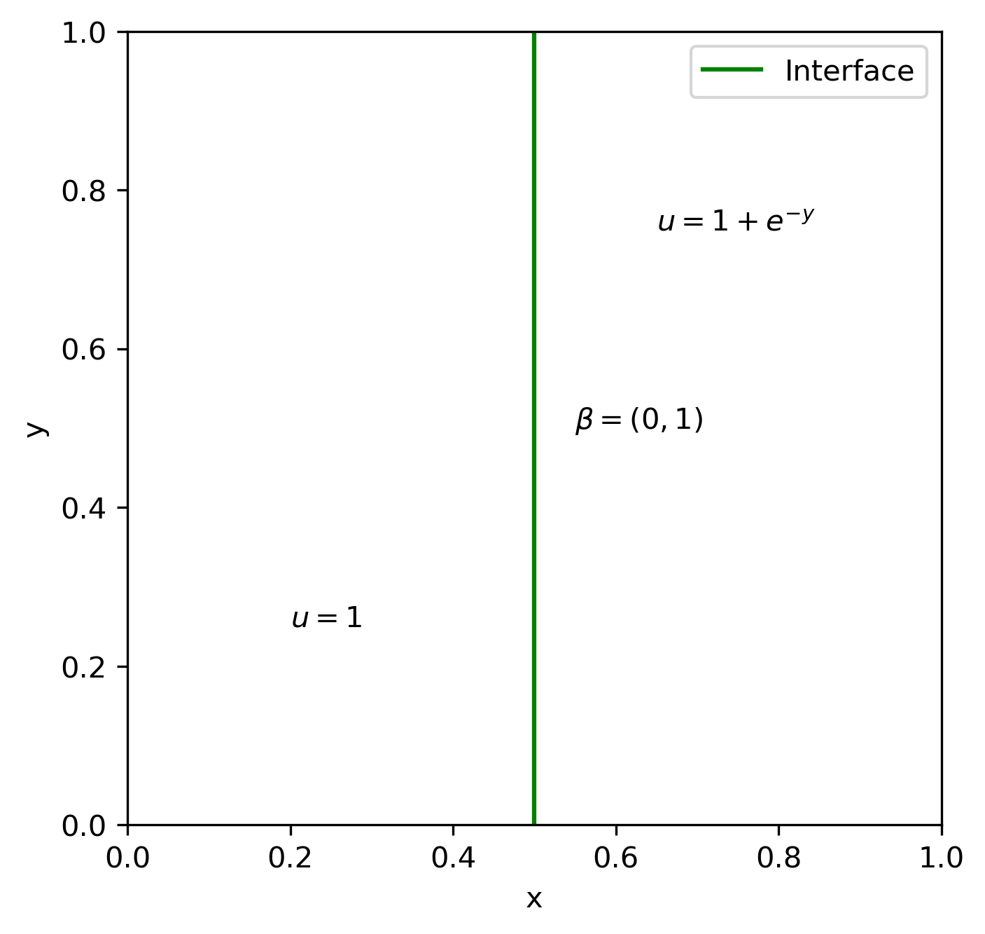
(a) The interface

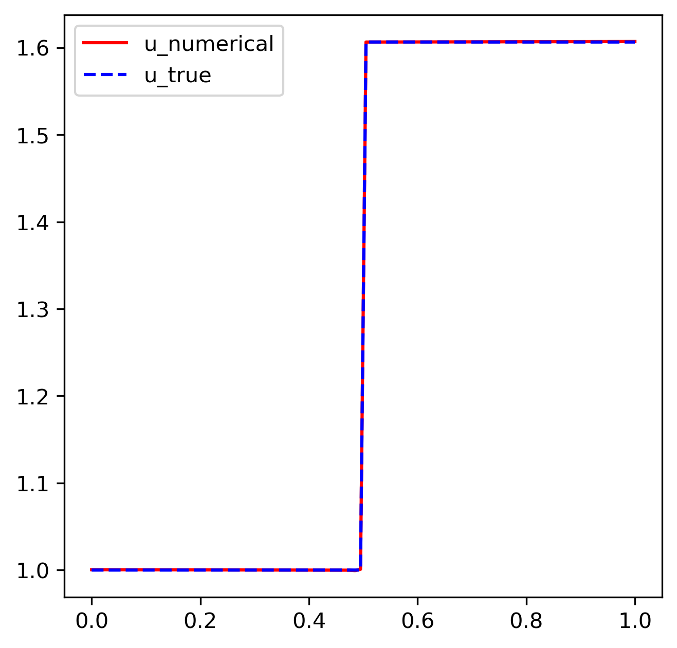
(b) The trace of Figure 2(d) on $y=0.5$

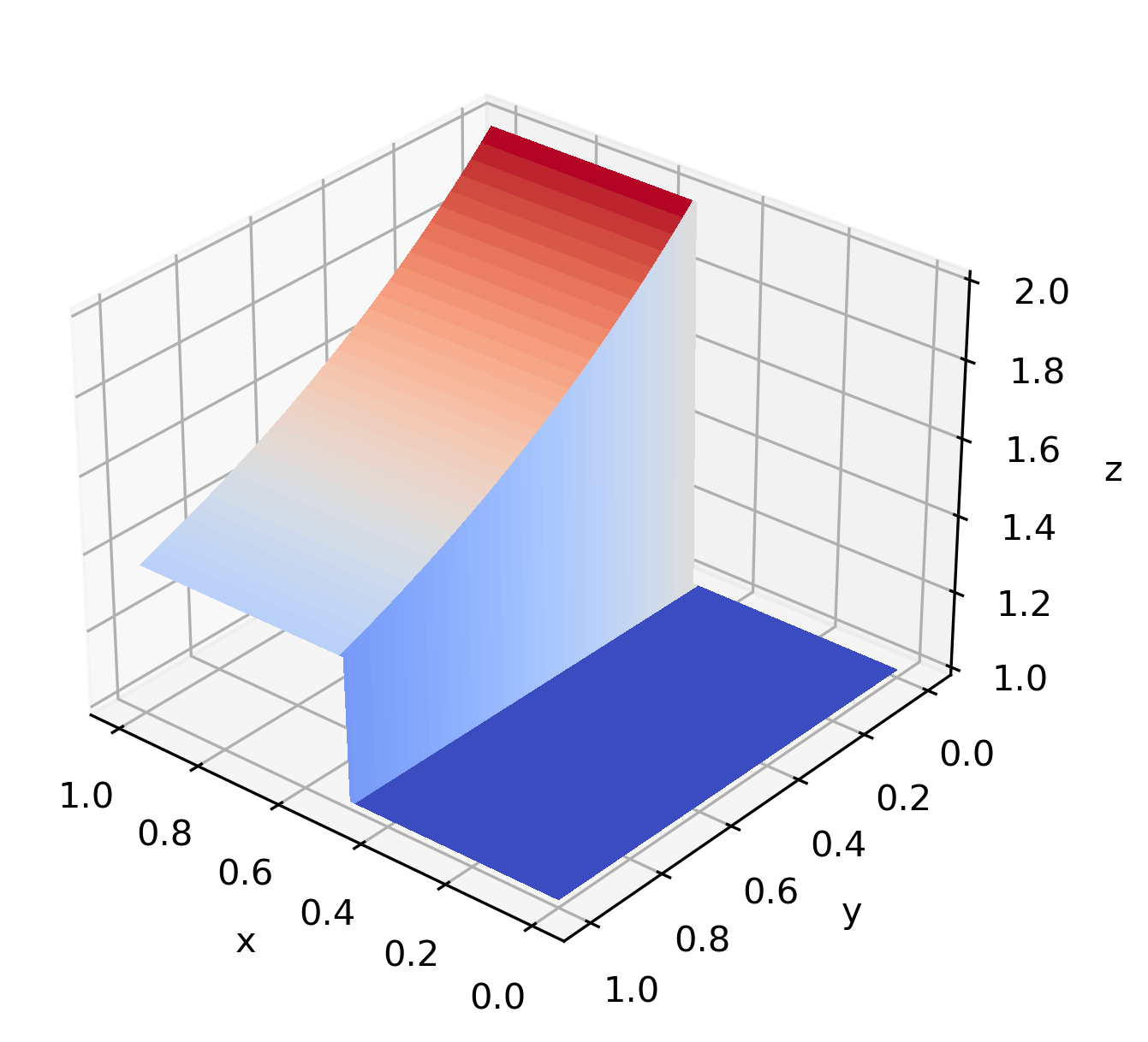
(c) The exact solution

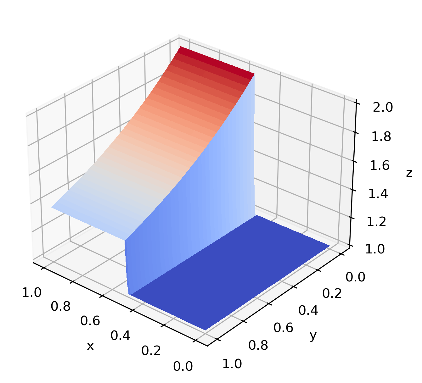
(d) A 2–20–20–1 ReLU NN function approximation

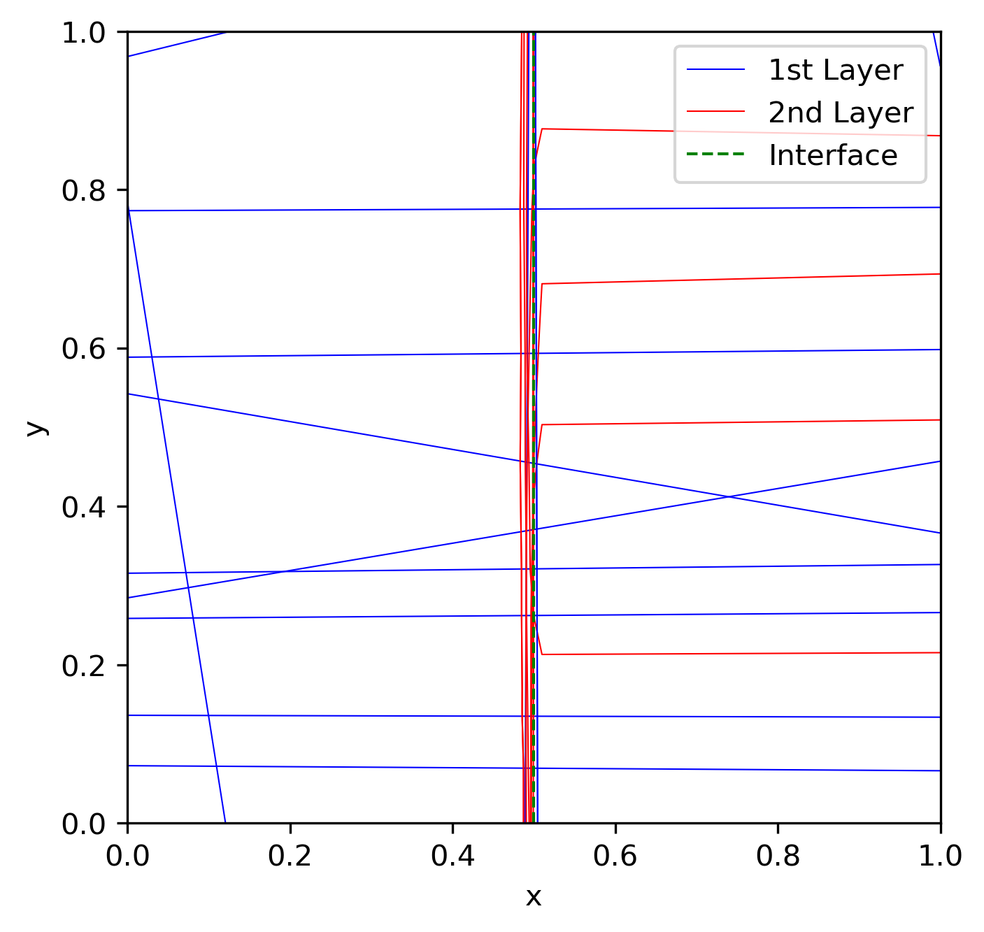
(e) The breaking hyperplanes of the approximation in Figure 2(d)

Figure 2: Approximation results of the problem in Section 4.1

Table 1: Relative errors of the problem in Section 4.1

Network structure	$\frac{\|u-{u}^{{}_{N}}_{{}_{\cal T}}\|_{0}}{\|u\|_{0}}$	$\frac{{\left|\kern-0.75346pt\left|\kern-0.75346pt\left|u-{u}^{{}_{N}}_{{}_{\cal T}}\right|\kern-0.75346pt\right|\kern-0.75346pt\right|}_{\bm{\beta}}}{{\left|\kern-0.75346pt\left|\kern-0.75346pt\left|u\right|\kern-0.75346pt\right|\kern-0.75346pt\right|}_{\bm{\beta}}}$	$\frac{\mathcal{L}^{1/2}({u}^{{}_{N}}_{{}_{\cal T}},\bf f)}{\mathcal{L}^{1/2}({u}^{{}_{N}}_{{}_{\cal T}},\bf 0)}$	Parameters
2–20–20–1	0.037881	0.007044	0.005391	501

4.2 A problem with a piecewise smooth solution

This example is a modification of Section 4.1 by changing the inflow boundary condition to

$$\Gamma_{-} = \{(x,0):x\in(0,1)\}$$

$$\mbox{and }\,\,g(x,y) = \left\{\begin{array}[]{rl}0,&(x,y)\in\Gamma^{1}_{-}\equiv\{(x,0):x\in(0,1/2)\},\\[5.69054pt] 2,&(x,y)\in\Gamma^{2}_{-}=\Gamma_{-}\setminus\Gamma_{-}^{1},\end{array}\right.$$

respectively. The exact solution of this test problem is

(19) $$u(x,y)=\left\{\begin{array}[]{rl}1-e^{-y},&(x,y)\in\Omega_{1},\\[5.69054pt] 1+e^{-y},&(x,y)\in\Omega_{2}.\end{array}\right.$$

50000 iterations were implemented with 2–20–20–1 ReLU NN functions. The numerical results are presented in Figs. 3 and 2. Unlike the previous test problem, the exact solution (Fig. 3(c)) consists of two non-constant smooth parts. The LSNN method is capable of approximating the solution accurately without oscillation (Figs. 3(b), 3(c), 3(d), and 2). The 3-layer ReLU NN function approximation has a partition (Fig. 3(e)) similar to that in Section 4.1 with the second-layer breaking hyperplanes on both sides for approximating the two non-constant smooth parts of the solution.

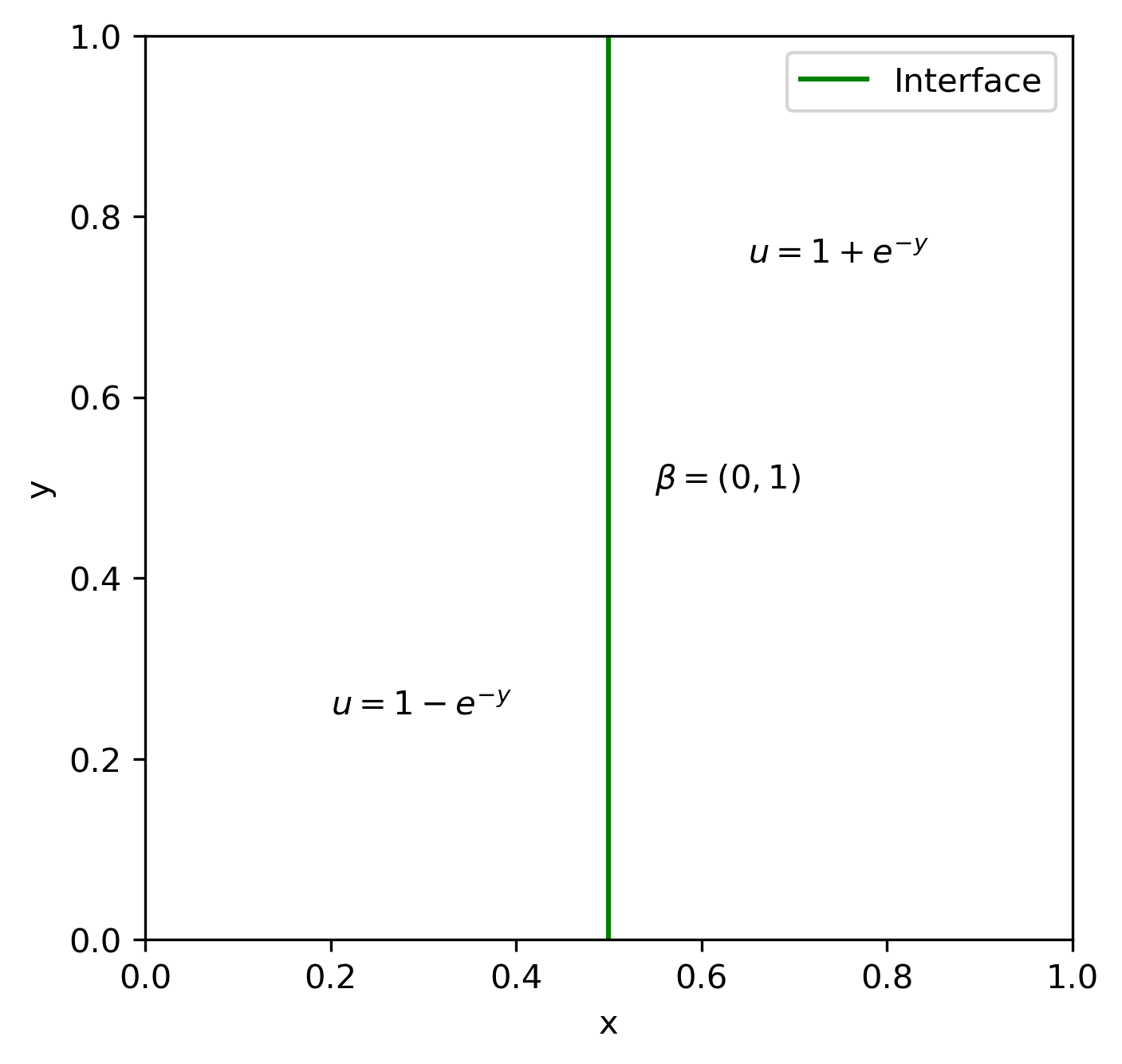
(a) The interface

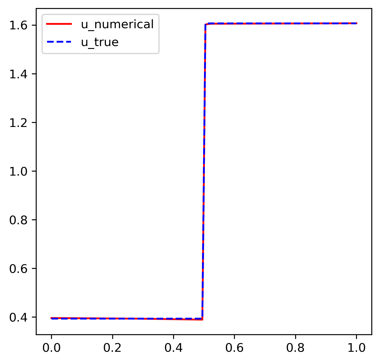
(b) The trace of Figure 3(d) on $y=0.5$

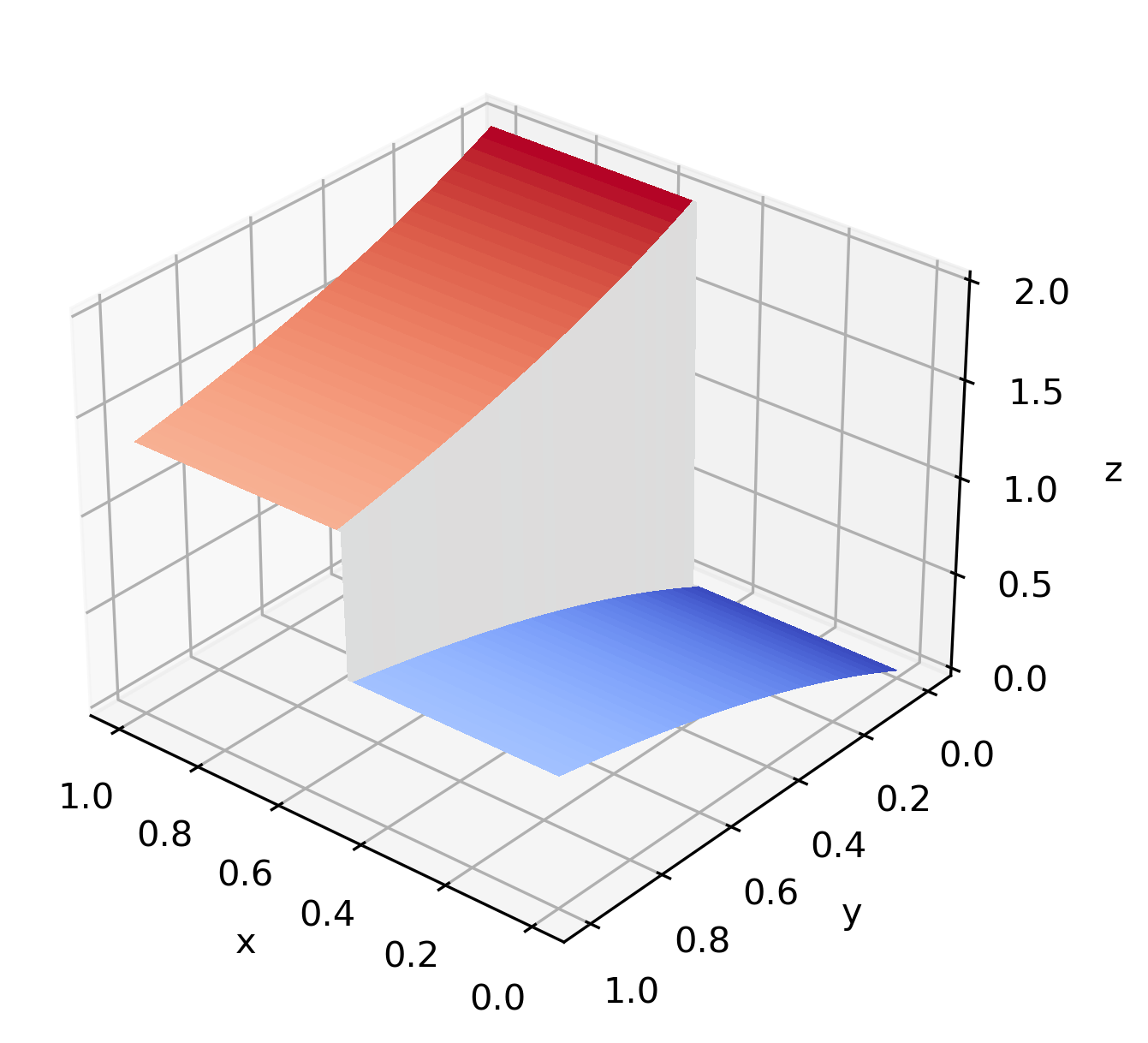
(c) The exact solution

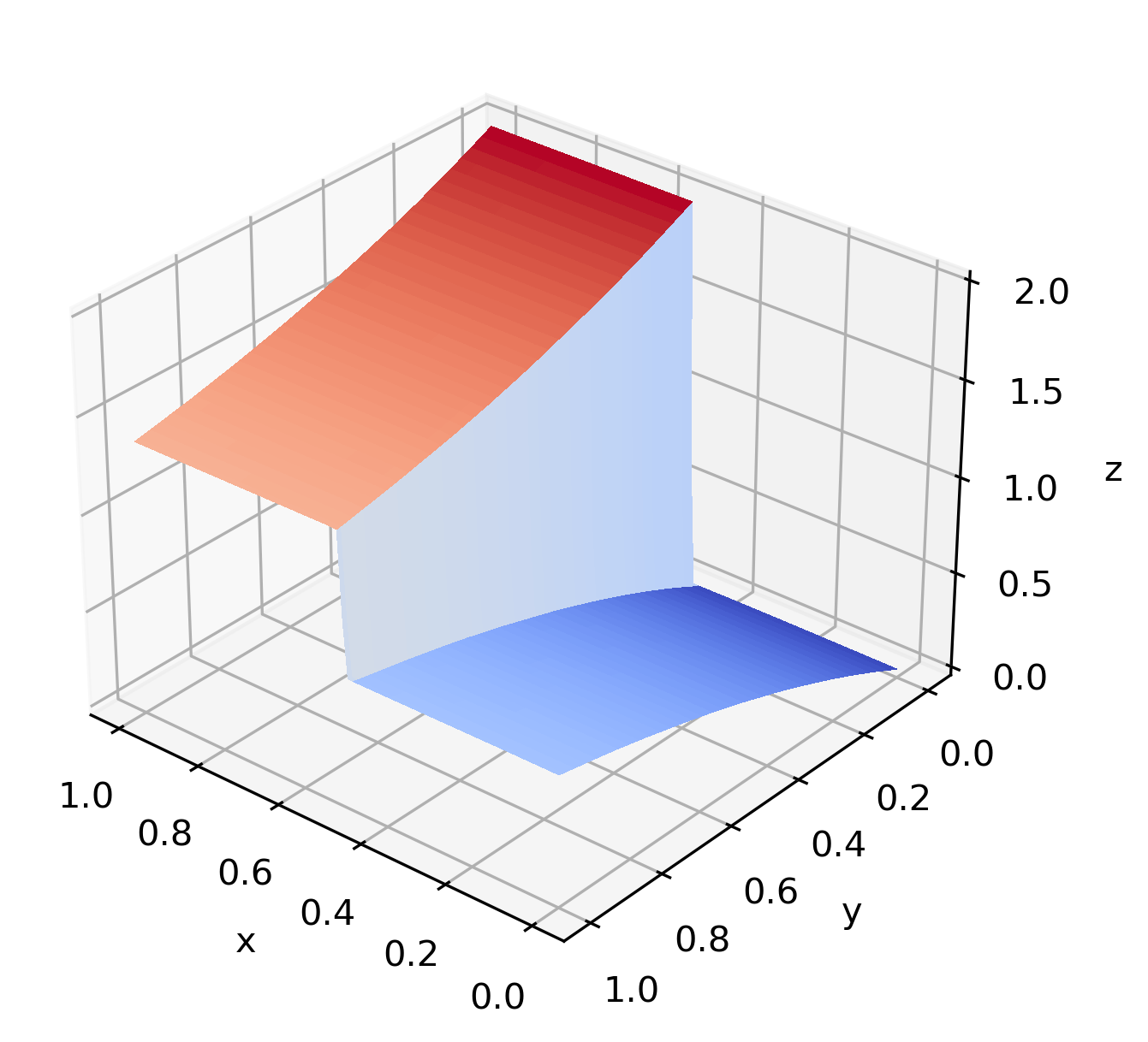
(d) A 2–20–20–1 ReLU NN function approximation

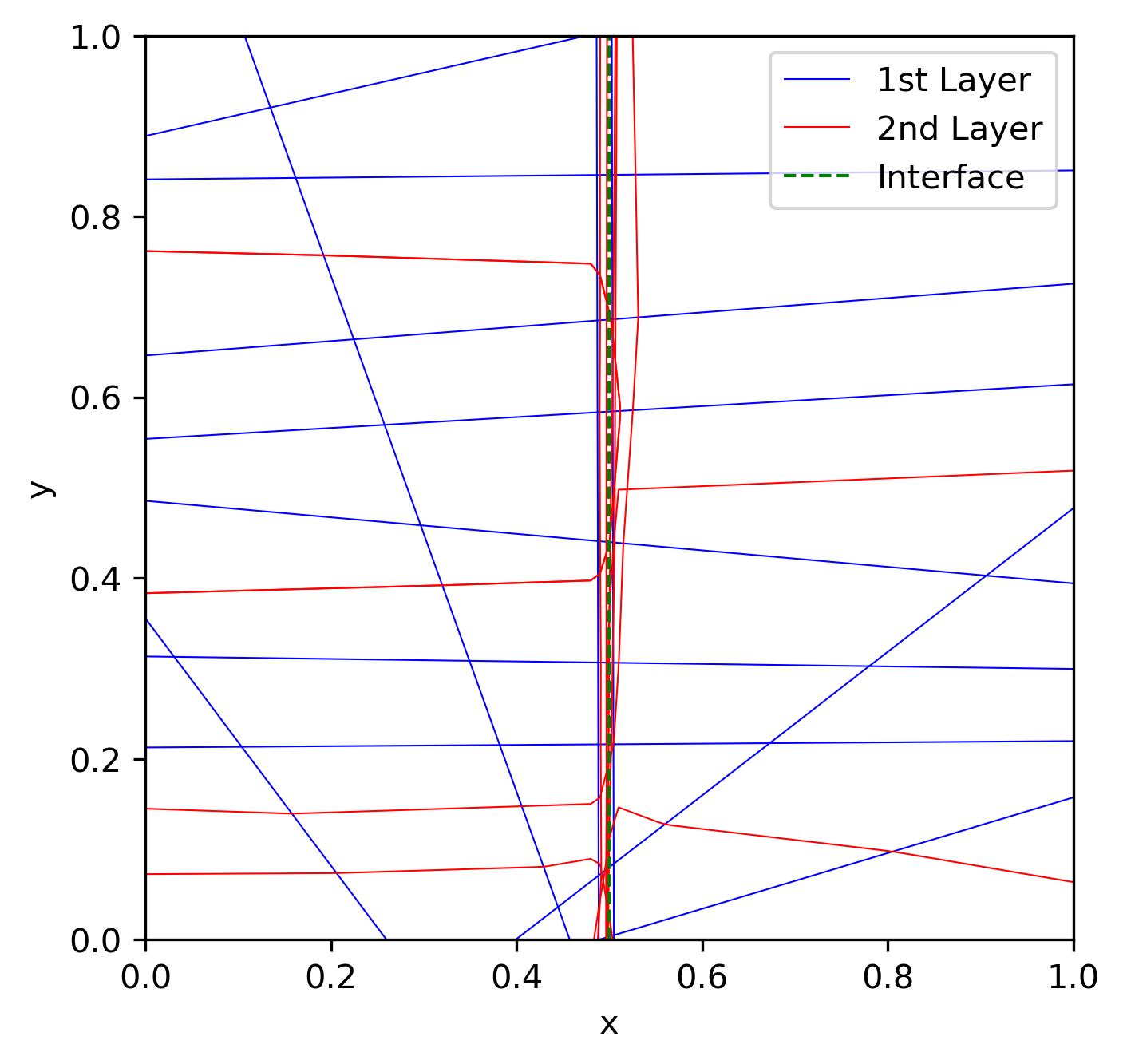
(e) The breaking hyperplanes of the approximation in Figure 3(d)

Figure 3: Approximation results of the problem in Section 4.2

Table 2: Relative errors of the problem in Section 4.2

Network structure	$\frac{\|u-{u}^{{}_{N}}_{{}_{\cal T}}\|_{0}}{\|u\|_{0}}$	$\frac{{\left|\kern-0.75346pt\left|\kern-0.75346pt\left|u-{u}^{{}_{N}}_{{}_{\cal T}}\right|\kern-0.75346pt\right|\kern-0.75346pt\right|}_{\bm{\beta}}}{{\left|\kern-0.75346pt\left|\kern-0.75346pt\left|u\right|\kern-0.75346pt\right|\kern-0.75346pt\right|}_{\bm{\beta}}}$	$\frac{\mathcal{L}^{1/2}({u}^{{}_{N}}_{{}_{\cal T}},\bf f)}{\mathcal{L}^{1/2}({u}^{{}_{N}}_{{}_{\cal T}},\bf 0)}$	Parameters
2–20–20–1	0.078036	0.013157	0.010386	501

4.3 A problem with a piecewise smooth inflow boundary

This example is again a modification of Section 4.1 by changing the inflow boundary condition to

$$\Gamma_{-} = \{(x,0):x\in(0,1)\}$$

$$\mbox{and }\,\,g(x,y) = \left\{\begin{array}[]{rl}1-\sin(2\pi x),&(x,y)\in\Gamma^{1}_{-}\equiv\{(x,0):x\in(0,1/2)\},\\[5.69054pt] 5/2-x,&(x,y)\in\Gamma^{2}_{-}=\Gamma_{-}\setminus\Gamma_{-}^{1},\end{array}\right.$$

respectively. The exact solution of this test problem is

(21) $$u(x,y)=\left\{\begin{array}[]{rl}1-\sin(2\pi x)e^{-y},&(x,y)\in\Omega_{1},\\[5.69054pt] 1+(3/2-x)e^{-y},&(x,y)\in\Omega_{2}.\end{array}\right.$$

100000 iterations were implemented with 2–40–40–1 ReLU NN functions. The numerical results are presented in Figs. 4 and 3. Since the solution on the inflow boundary consists of two non-constant smooth curves, we increased the number of hidden neurons to obtain a more accurate solution. Figs. 4(c), 4(d), and 3 show that the approximation is accurate pointwise and in average. The traces (Fig. 4(b)) on $y=0.5$ exhibit no oscillation and we note a few corners on the curve, verifying that the ReLU NN function approximation is a CPWL function. The partition generated by the breaking hyperplanes (Fig. 4(e)) of the approximation shows how the exact solution was approximated.

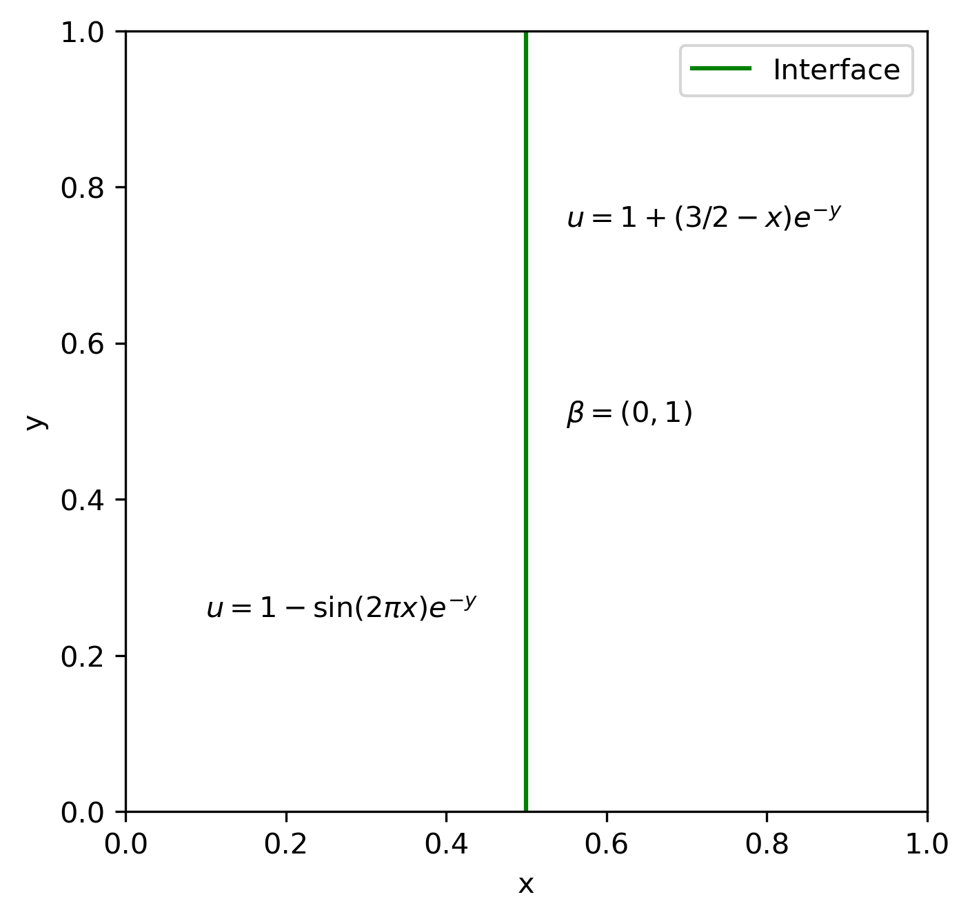
(a) The interface

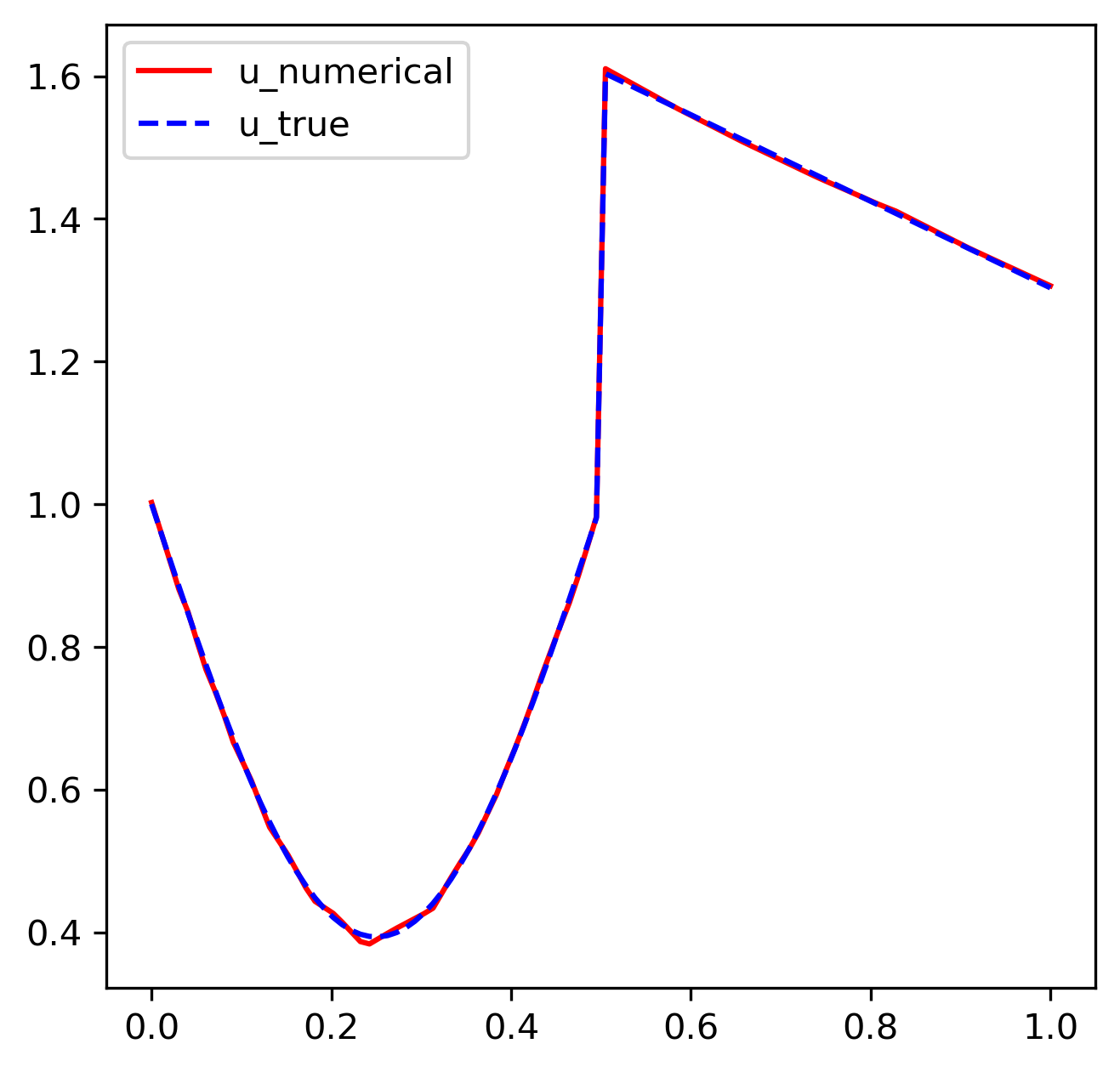
(b) The trace of Figure 4(d) on $y=0.5$

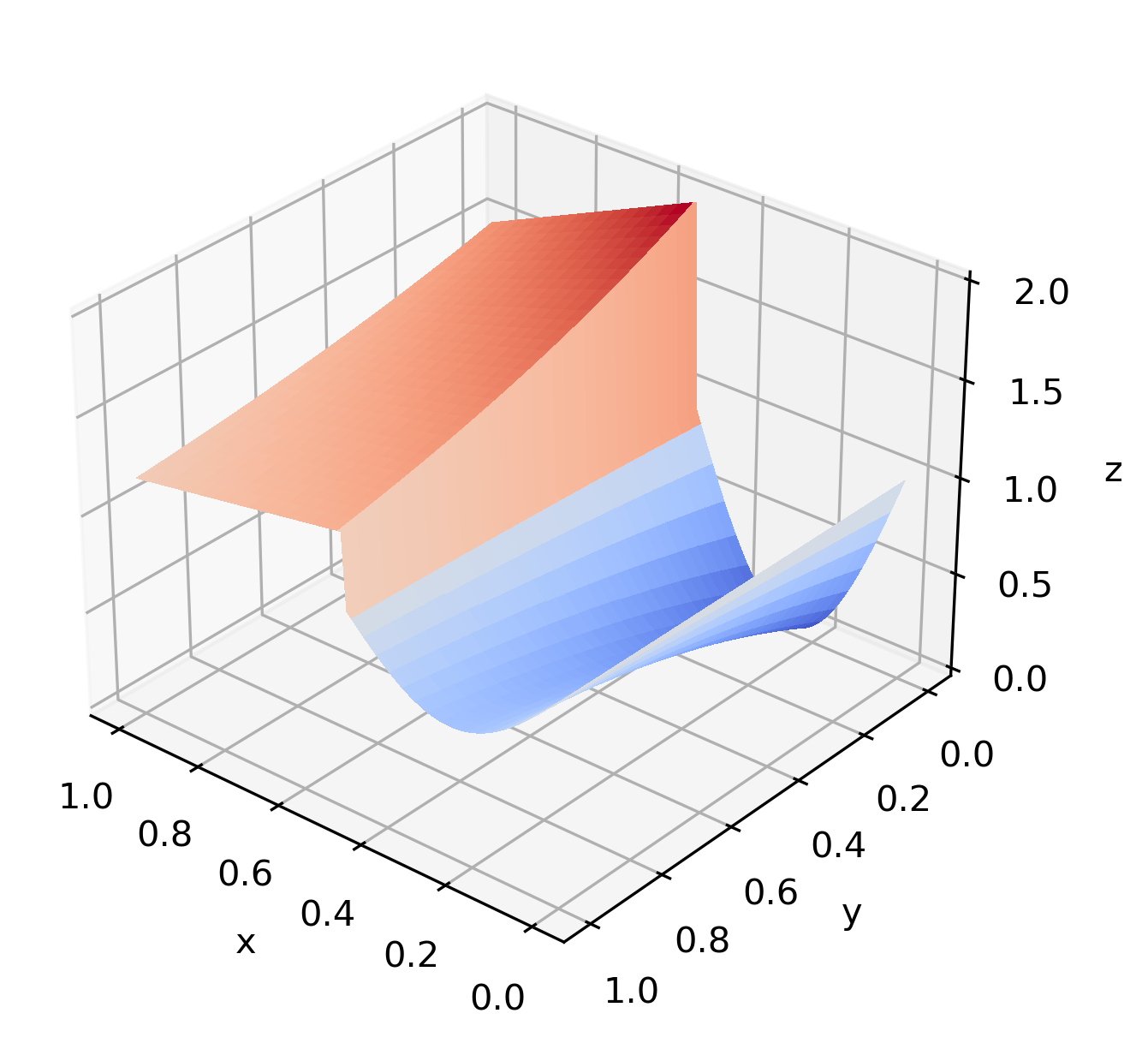
(c) The exact solution

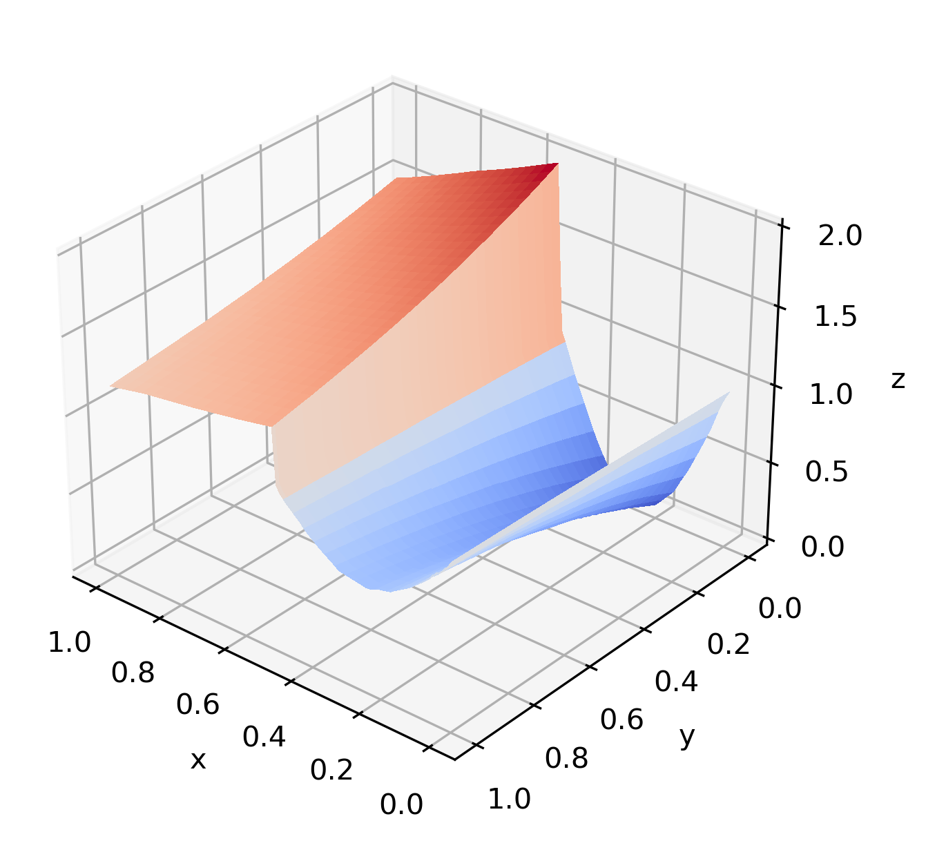
(d) A 2–40–40–1 ReLU NN function approximation

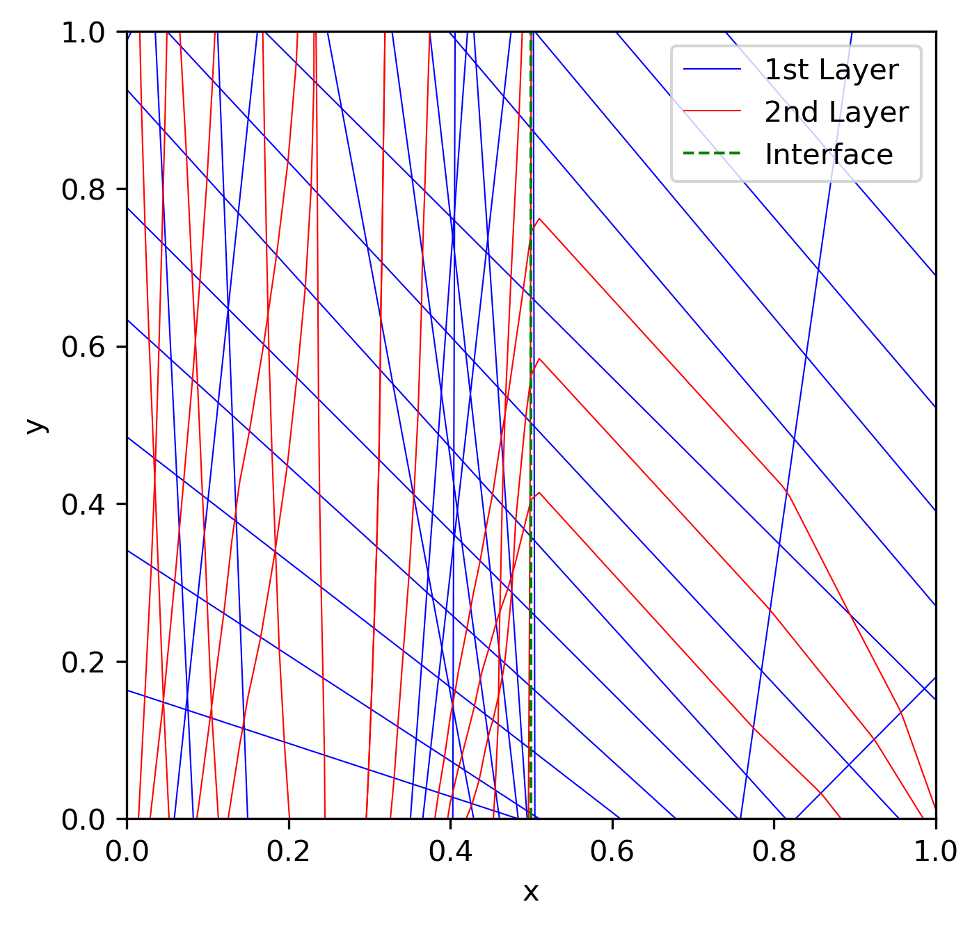
(e) The breaking hyperplanes of the approximation in Figure 4(d)

Figure 4: Approximation results of the problem in Section 4.3

Table 3: Relative errors of the problem in Section 4.3

Network structure	$\frac{\|u-{u}^{{}_{N}}_{{}_{\cal T}}\|_{0}}{\|u\|_{0}}$	$\frac{{\left|\kern-0.75346pt\left|\kern-0.75346pt\left|u-{u}^{{}_{N}}_{{}_{\cal T}}\right|\kern-0.75346pt\right|\kern-0.75346pt\right|}_{\bm{\beta}}}{{\left|\kern-0.75346pt\left|\kern-0.75346pt\left|u\right|\kern-0.75346pt\right|\kern-0.75346pt\right|}_{\bm{\beta}}}$	$\frac{\mathcal{L}^{1/2}({u}^{{}_{N}}_{{}_{\cal T}},\bf f)}{\mathcal{L}^{1/2}({u}^{{}_{N}}_{{}_{\cal T}},\bf 0)}$	Parameters
2–40–40–1	0.041491	0.016480	0.012733	1801

4.4 A problem with a piecewise constant advection velocity field

Let $\bar{\Omega}=\bar{\Upsilon}_{1}\cup\bar{\Upsilon}_{2}$ and

$$\Upsilon_{1}=\{(x,y)\in\Omega:y\geq x\}\text{ and }\Upsilon_{2}=\Omega\setminus\Upsilon_{1}.$$

The advective velocity field is a piecewise constant field given by

(22) $$\bm{\beta}(x,y)=\left\{\begin{array}[]{rl}(-1,\sqrt{2}-1)^{T},&(x,y)\in\Upsilon_{1},\\[5.69054pt] (1-\sqrt{2},1)^{T},&(x,y)\in\Upsilon_{2}.\end{array}\right.$$

The inflow boundary and the inflow boundary condition are given by

$$\Gamma_{-} = \{(1,y):y\in(0,1)\}\cup\{(x,0):x\in(0,1)\}$$

$$\mbox{and }\,\,g(x,y) = \left\{\begin{array}[]{rl}x\exp(x/(\sqrt{2}-1)),&(x,y)\in\Gamma^{1}_{-}\equiv\{(x,0):x\in(0,1)\},\\[5.69054pt] (11+(\sqrt{2}-1)y)\exp(1/(\sqrt{2}-1)),&(x,y)\in\Gamma^{2}_{-}=\Gamma_{-}\setminus\Gamma_{-}^{1},\end{array}\right.$$

respectively. Let

$$\widehat{\Upsilon}_{11}=\{(x,y)\in\Upsilon_{1}:y<(1-\sqrt{2})x+1\},\,\,\widehat{\Upsilon}_{12}=\Upsilon_{1}\setminus\widehat{\Upsilon}_{11},\\[5.69054pt] \widehat{\Upsilon}_{21}=\{(x,y)\in\Upsilon_{2}:y<\tfrac{1}{1-\sqrt{2}}(x-1)\},\text{ and }\widehat{\Upsilon}_{22}=\Upsilon_{2}\setminus\widehat{\Upsilon}_{21}.$$

The exact solution of this test problem is

(24) $$u(x,y)=\left\{\begin{array}[]{rl}(y+(\sqrt{2}-1)x)\exp(\sqrt{2}x+y),&(x,y)\in\widehat{\Upsilon}_{11},\\[5.69054pt] (y+(\sqrt{2}-1)x+10)\exp(\sqrt{2}x+y),&(x,y)\in\widehat{\Upsilon}_{12},\\[5.69054pt] (x+(\sqrt{2}-1)y)\exp(x/(\sqrt{2}-1)),&(x,y)\in\widehat{\Upsilon}_{21},\\[5.69054pt] (x+(\sqrt{2}-1)y+10)\exp(x/(\sqrt{2}-1)),&(x,y)\in\widehat{\Upsilon}_{22}.\end{array}\right.$$

300000 iterations were implemented with 2–450–1 and 2–40–40–1 ReLU NN functions. The numerical results are presented in Figs. 5 and 4. This example compares the approximation differences with the one-hidden-layer NN (a universal approximator) with the same number of degrees of freedom. The exact solution (Fig. 5(b)) consists of four non-constant smooth parts and has a non-constant jump along two connected line segments (Fig. 5(a)). The traces (Fig. 5(f)) of the exact and numerical solutions, the approximation (Fig. 5(d)), and Table 4 indicate that the 3-layer ReLU NN function approximation is accurate pointwise and in average. Most of the second-layer breaking hyperplanes (Fig. 5(h)) are along the discontinuous interface, which correspond to the sharp transition layer of the approximation for the jump. On the other hand, Figs. 5(c), 5(e), 5(g), and 4 show that the one-hidden-layer NN failed to approximate the solution, especially around the interface.

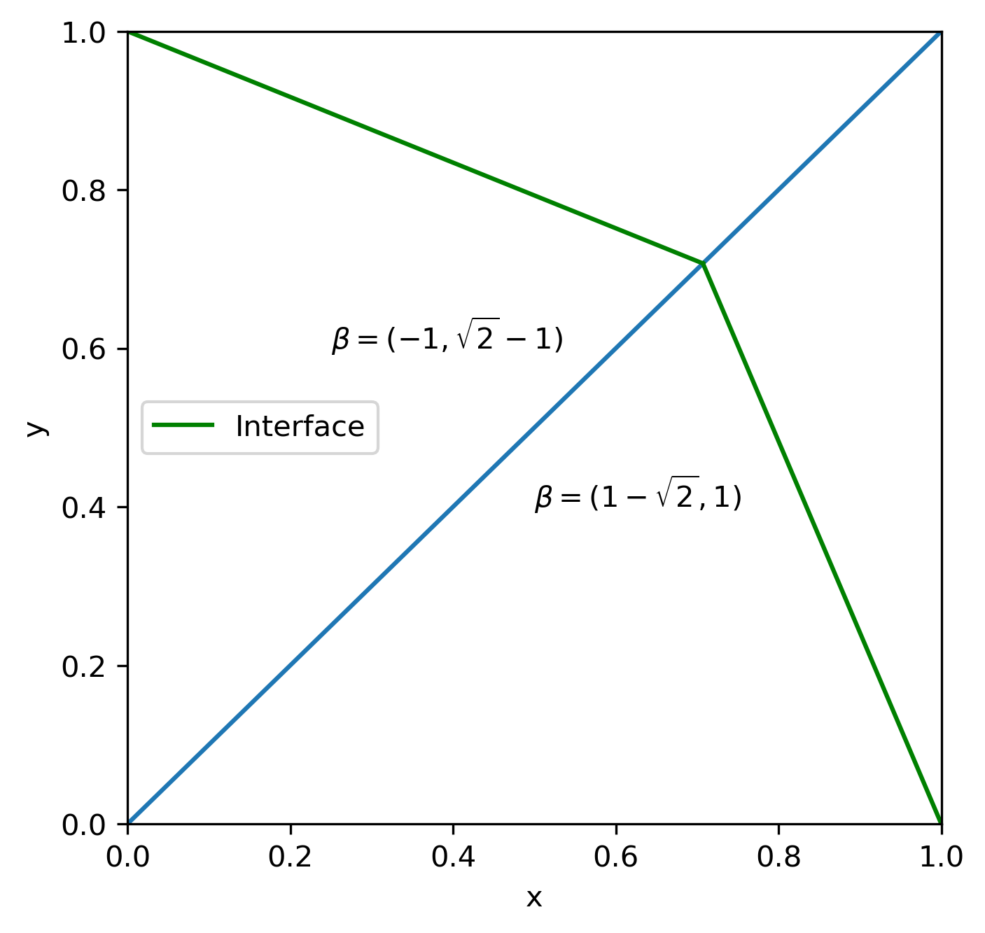
(a) The interface

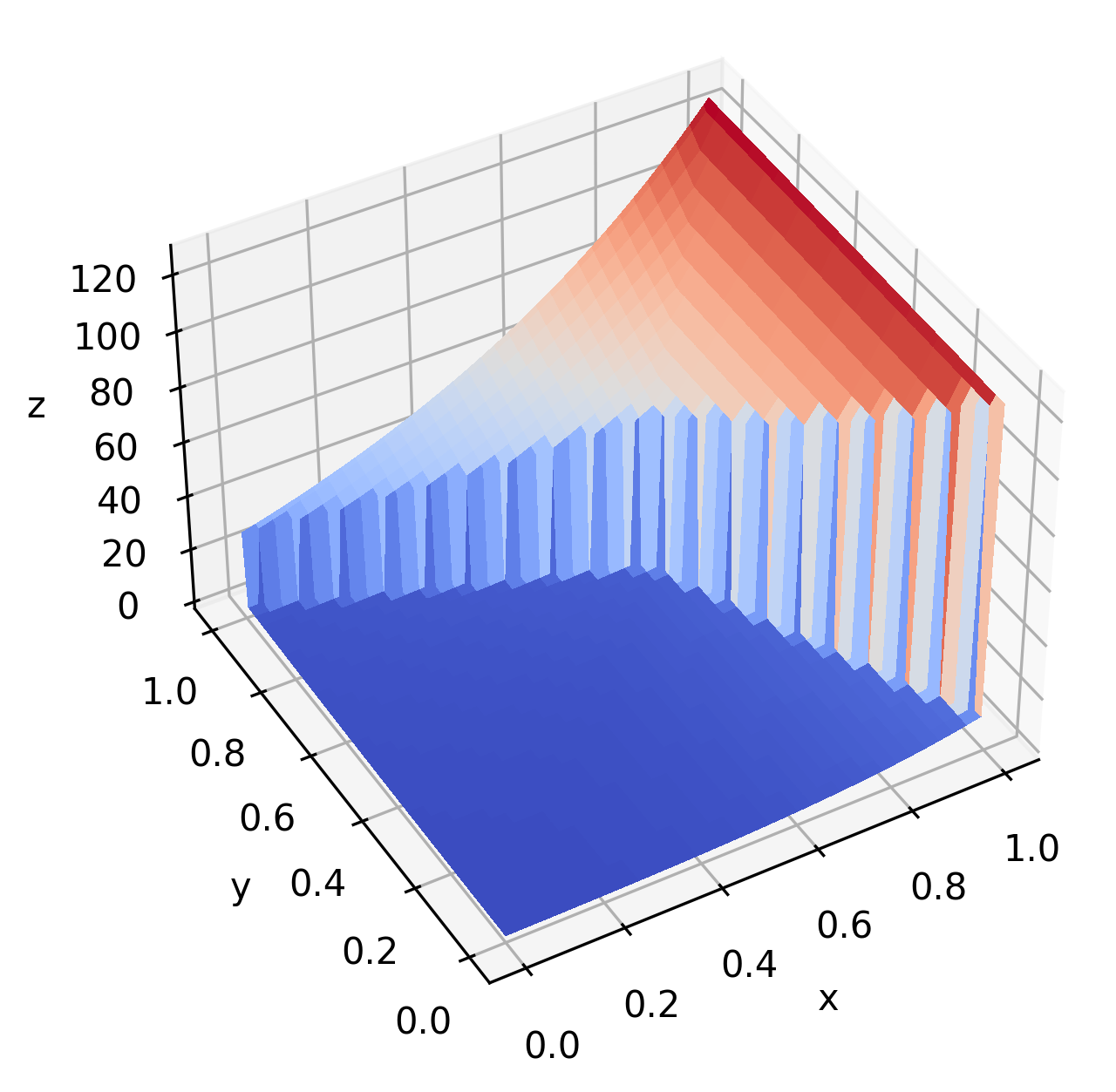
(b) The exact solution

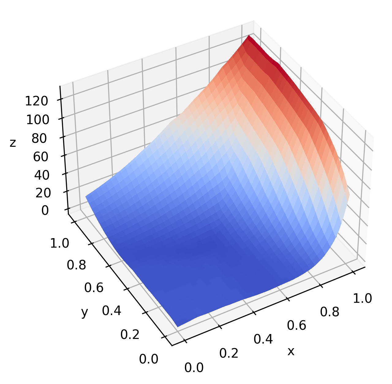
(c) A 2–450–1 ReLU NN function approximation

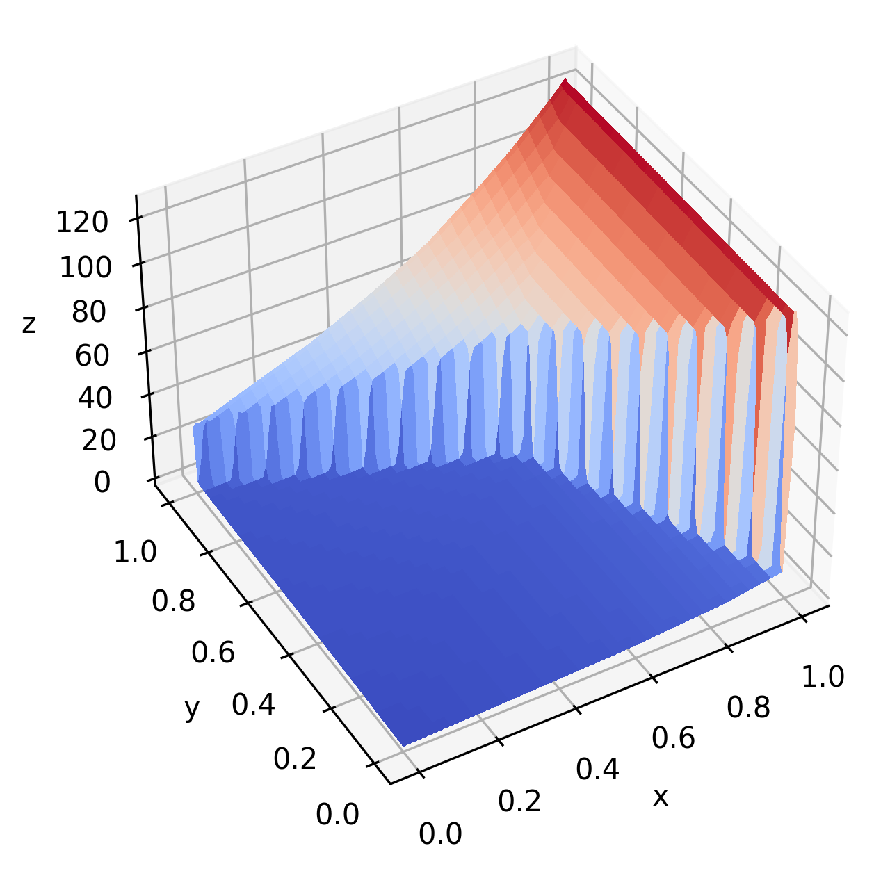
(d) A 2–40–40–1 ReLU NN function approximation

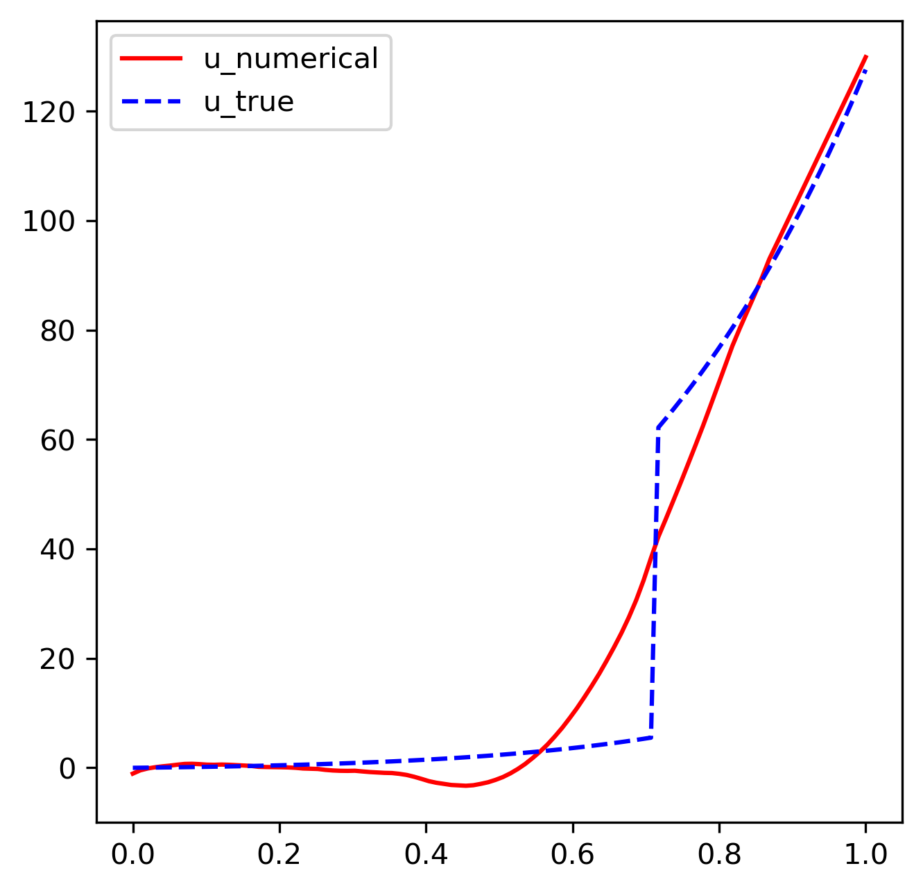
(e) The trace of Figure 5(c) on $y=x$

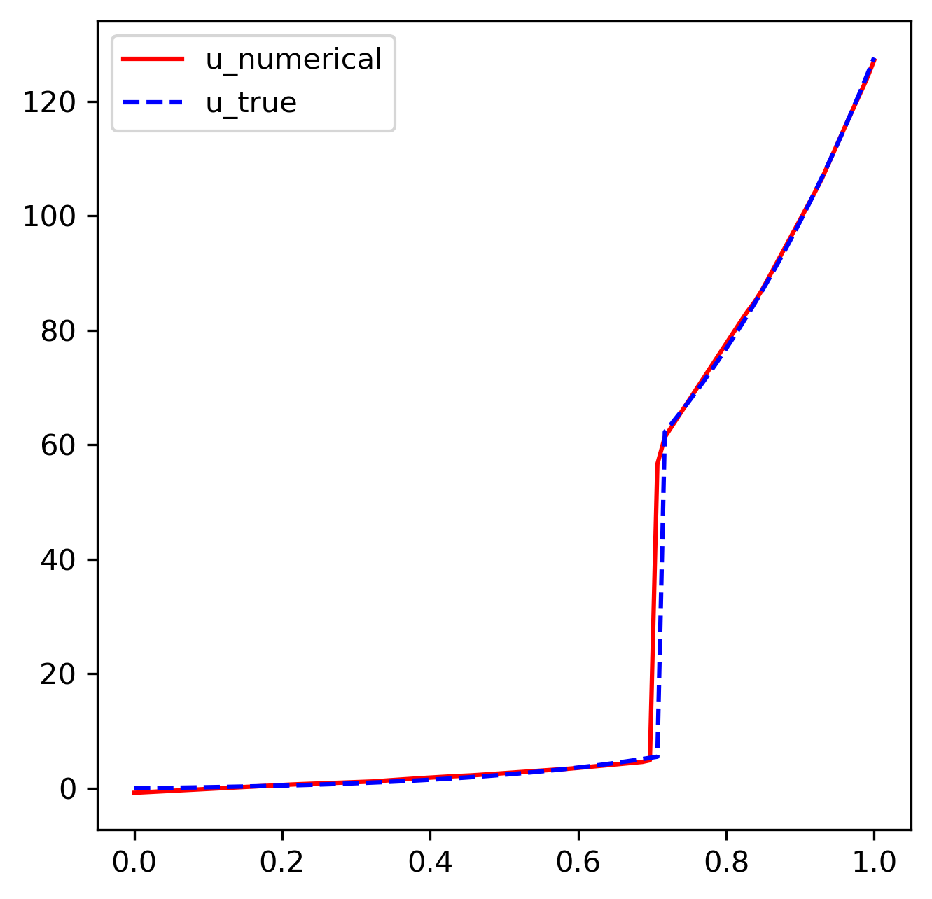
(f) The trace of Figure 5(d) on $y=x$

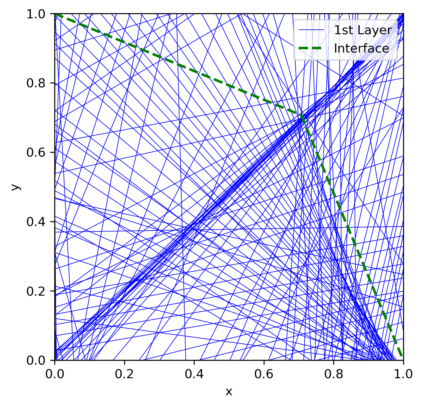
(g) The breaking hyperplanes of the approximation in Figure 5(c)

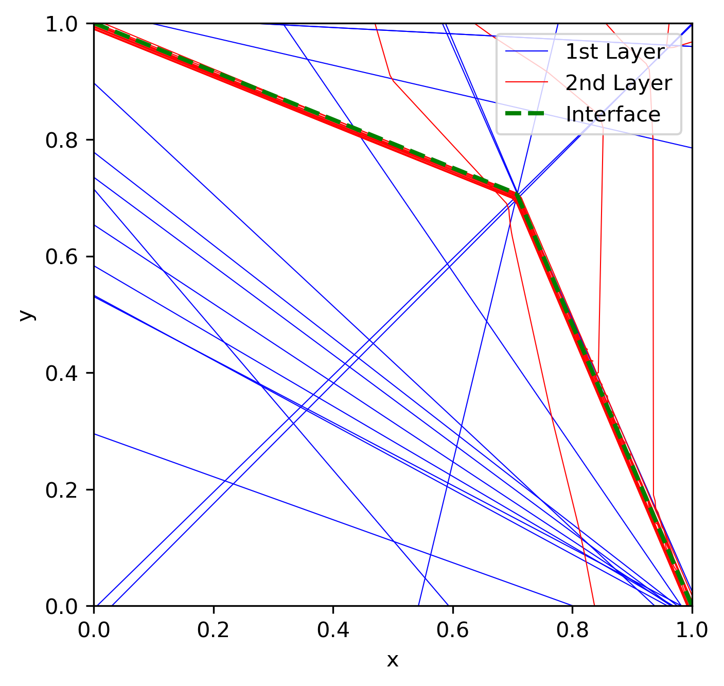
(h) The breaking hyperplanes of the approximation in Figure 5(d)

Figure 5: Approximation results of the problem in Section 4.4

Table 4: Relative errors of the problem in Section 4.4

Network structure	$\frac{\|u-{u}^{{}_{N}}_{{}_{\cal T}}\|_{0}}{\|u\|_{0}}$	$\frac{{\left|\kern-0.75346pt\left|\kern-0.75346pt\left|u-{u}^{{}_{N}}_{{}_{\cal T}}\right|\kern-0.75346pt\right|\kern-0.75346pt\right|}_{\bm{\beta}}}{{\left|\kern-0.75346pt\left|\kern-0.75346pt\left|u\right|\kern-0.75346pt\right|\kern-0.75346pt\right|}_{\bm{\beta}}}$	$\frac{\mathcal{L}^{1/2}({u}^{{}_{N}}_{{}_{\cal T}},\bf f)}{\mathcal{L}^{1/2}({u}^{{}_{N}}_{{}_{\cal T}},\bf 0)}$	Parameters
2–40–40–1	0.058884	0.073169	0.038245	1801
2–450–1	0.243956	0.258038	0.225756	1801

4.5 A problem with a variable advection velocity field

The advective velocity field is a variable field given by

(25) $$\bm{\beta}(x,y)=(1,2x),\,\,(x,y)\in\Omega.$$

The inflow boundary and the inflow boundary condition are given by

$$\Gamma_{-} = \{(0,y):y\in(0,1)\}\cup\{(x,0):x\in(0,1)\}$$

$$\mbox{and }\,\,g(x,y) = \left\{\begin{array}[]{rl}y+2,&(x,y)\in\Gamma^{1}_{-}\equiv\{(0,y):y\in[\frac{1}{5},1)\},\\[5.69054pt] (y-x^{2})e^{-x},&(x,y)\in\Gamma^{2}_{-}=\Gamma_{-}\setminus\Gamma_{-}^{1},\end{array}\right.$$

respectively. The exact solution of this test problem is

(27) $$u(x,y)=\left\{\begin{array}[]{rl}(y-x^{2})e^{-x},&(x,y)\in\Omega_{1}\equiv\{(x,y)\in\Omega:y<x^{2}+\frac{1}{5}\},\\[5.69054pt] (y-x^{2}+2)e^{-x},&(x,y)\in\Omega_{2}=\Omega\setminus\Omega_{1}.\end{array}\right.$$

300000 iterations were implemented with 2–60–60–1 ReLU NN functions. The numerical results are presented in Figs. 6 and 5. We increased the number of hidden neurons and $\rho$ was set to $h/15$ in the finite difference quotient in Eq. 14 because of the jump along the curved interface (Fig. 6(a)). Although theoretical analysis on the convergence of the method in the case of a smooth interface was not conducted, Figs. 6(b), 6(c), 6(d), and 5 show that the LSNN method is still capable of approximating the discontinuous solution with the curved interface accurately without oscillation. Finally, again, most of the second-layer breaking hyperplanes are along the interface (Fig. 6(e)) to approximate the discontinuous jump.

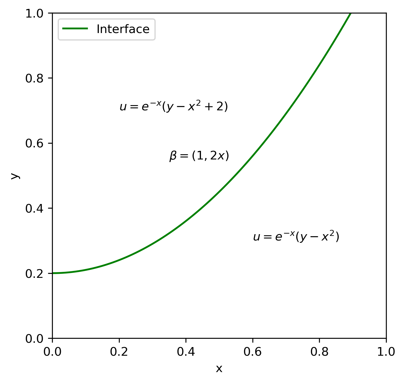
(a) The interface

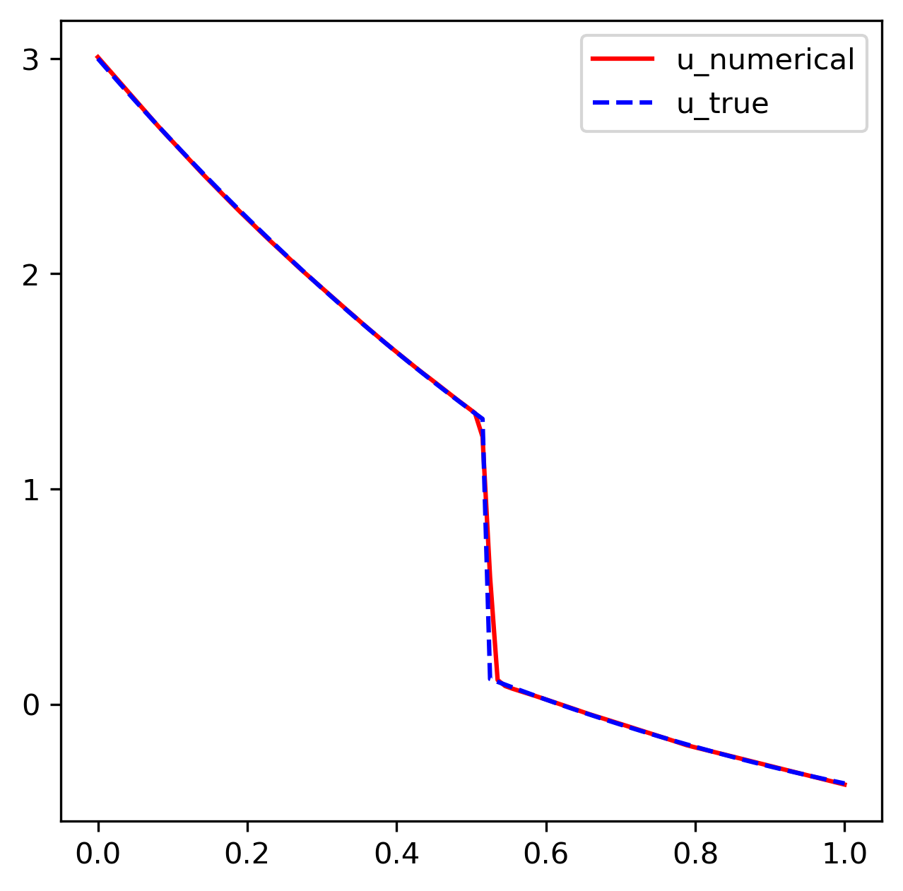
(b) The trace of Figure 6(d) on $y=1-x$

(c) The exact solution

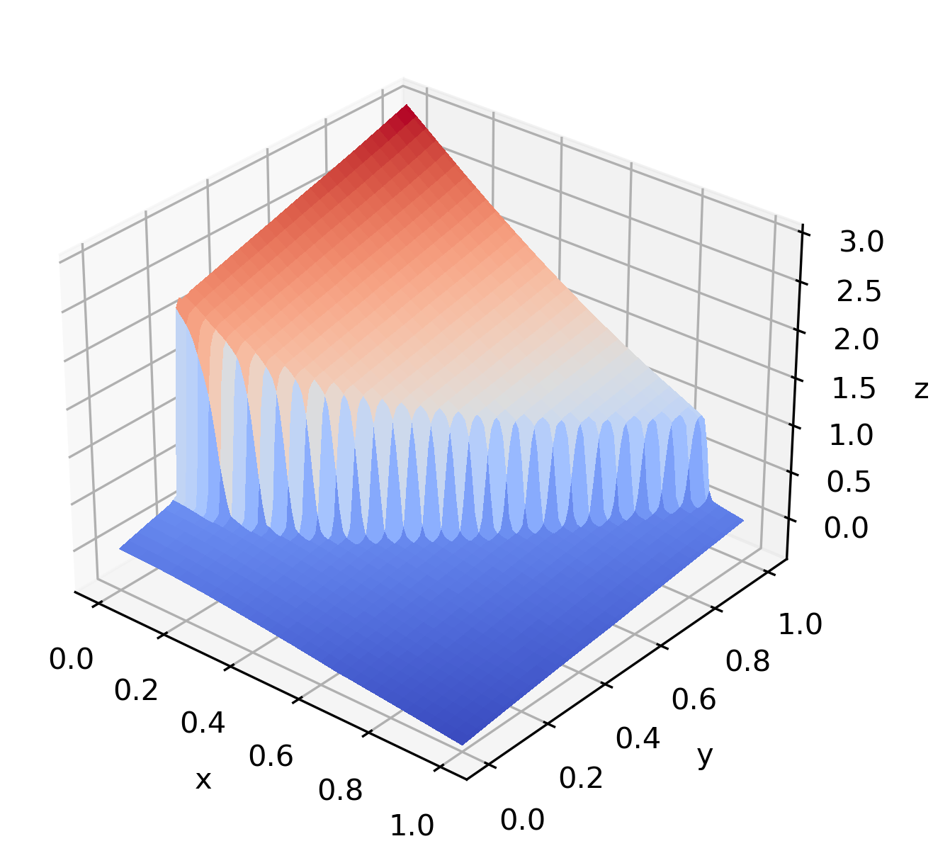
(d) A 2–60–60–1 ReLU NN function approximation

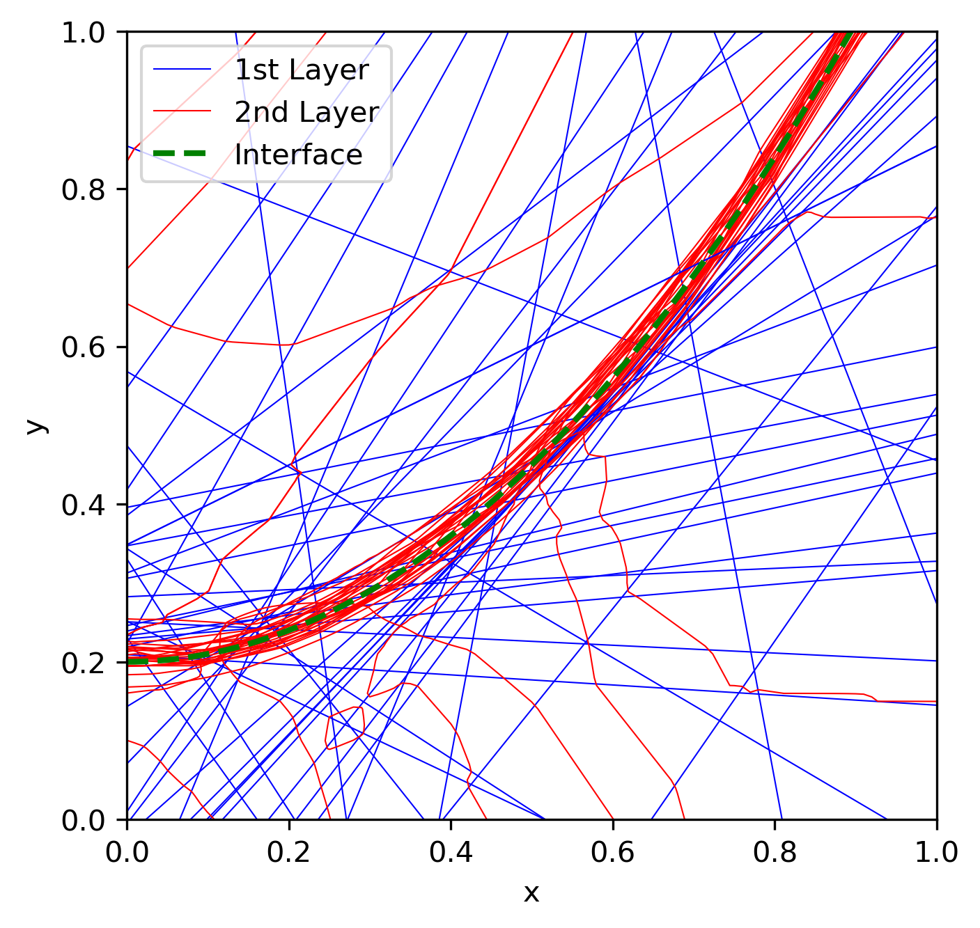
(e) The breaking hyperplanes of the approximation in Figure 6(d)

Figure 6: Approximation results of the problem in Section 4.5

Table 5: Relative errors of the problem in Section 4.5

Network structure	$\frac{\|u-{u}^{{}_{N}}_{{}_{\cal T}}\|_{0}}{\|u\|_{0}}$	$\frac{{\left|\kern-0.75346pt\left|\kern-0.75346pt\left|u-{u}^{{}_{N}}_{{}_{\cal T}}\right|\kern-0.75346pt\right|\kern-0.75346pt\right|}_{\bm{\beta}}}{{\left|\kern-0.75346pt\left|\kern-0.75346pt\left|u\right|\kern-0.75346pt\right|\kern-0.75346pt\right|}_{\bm{\beta}}}$	$\frac{\mathcal{L}^{1/2}({u}^{{}_{N}}_{{}_{\cal T}},\bf f)}{\mathcal{L}^{1/2}({u}^{{}_{N}}_{{}_{\cal T}},\bf 0)}$	Parameters
2–60–60–1	0.046528	0.049423	0.019995	3901

Now we present numerical results for a three-dimensional test problem with a constant advection velocity field whose solution is piecewise smooth along a plane segment with a non-constant jump. The test problem is defined on the domain $\Omega=(0,1)^{3}$, and approximation results are depicted on $z=0.505$.

4.6 A problem with a constant advection velocity field

The advective velocity field is a constant field given by

(28) $$\bm{\beta}(x,y,z)=(1,0,0),\,\,(x,y,z)\in\Omega.$$

The inflow boundary and the inflow boundary condition are given by

$$\Gamma_{-} = \{(0,y,z):y,z\in(0,1)\}$$

$$\mbox{and }\,\,g(x,y,z) = \left\{\begin{array}[]{rl}1-4y,&(x,y,z)\in\Gamma^{1}_{-}\equiv\{(0,y,z)\in\Gamma_{-}:y<\frac{1}{2}\},\\[5.69054pt] 5-4y,&(x,y,z)\in\Gamma^{2}_{-}=\Gamma_{-}\setminus\Gamma_{-}^{1},\end{array}\right.$$

respectively. The exact solution of this test problem is

(30) $$u(x,y,z)=\left\{\begin{array}[]{rl}1-4ye^{-x},&(x,y,z)\in\Omega_{1}\equiv\{(x,y,z)\in\Omega:y<\frac{1}{2}\},\\[5.69054pt] 1+(4-4y)e^{-x},&(x,y,z)\in\Omega_{2}=\Omega\setminus\Omega_{1}.\end{array}\right.$$

100000 iterations were implemented with 3–30–30–1 ReLU NN functions (depth $\lceil\log_{2}(d+1)\rceil+1=3$ for $d=3$). The numerical results are presented in Figs. 7 and 6. The exact solution (Fig. 7(c)) is discontinuous along the plane segment $y=0.5$ (Fig. 7(a)), and was approximated accurately by the 3-layer NN (Figs. 7(b), 7(d), and 6). The behavior of the breaking hyperplanes (Fig. 7(e)) is similar to those of the previous examples around the discontinuous interface and on the subdomains.

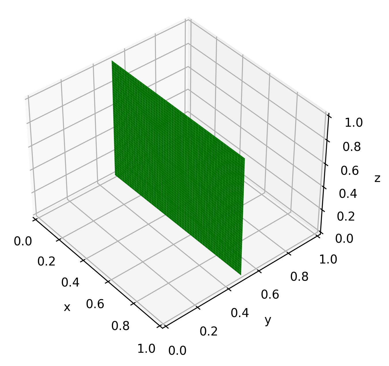
(a) The interface

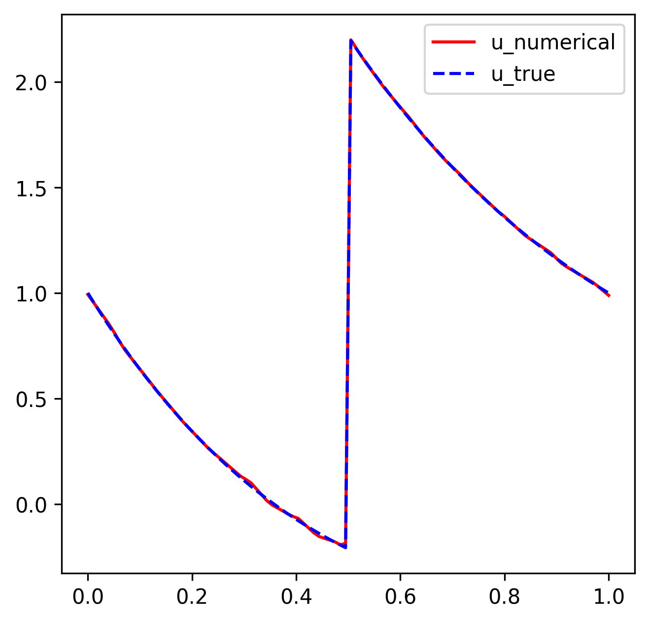
(b) The trace of Figure 7(d) on $y=x$

(c) The exact solution

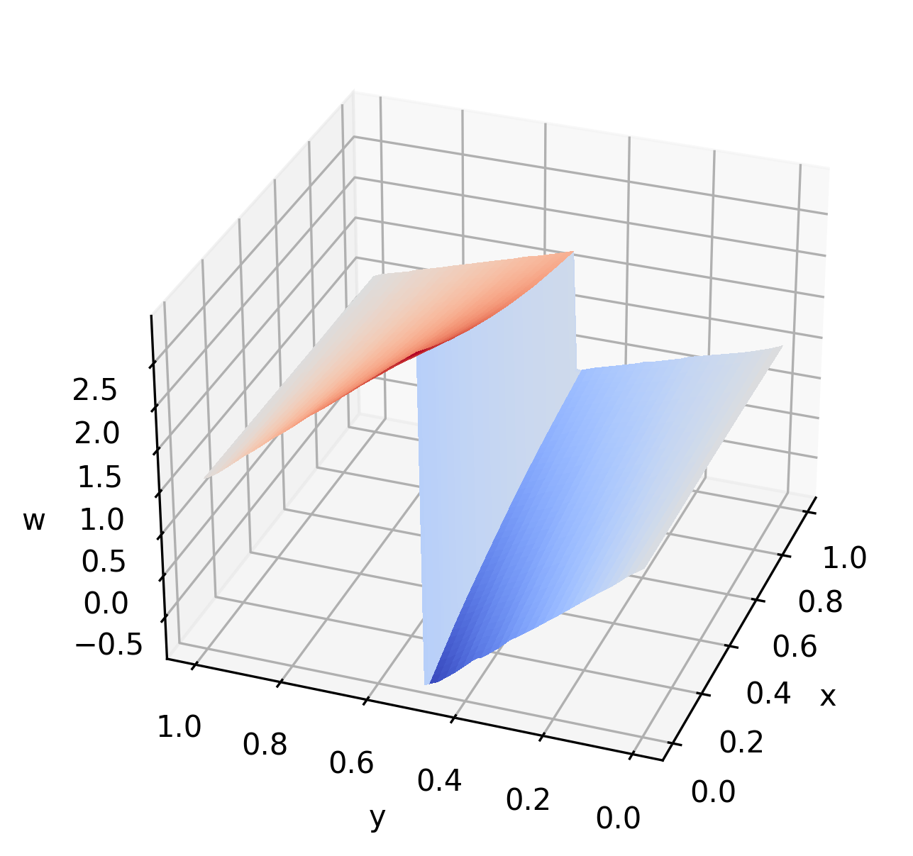
(d) A 3–30–30–1 ReLU NN function approximation

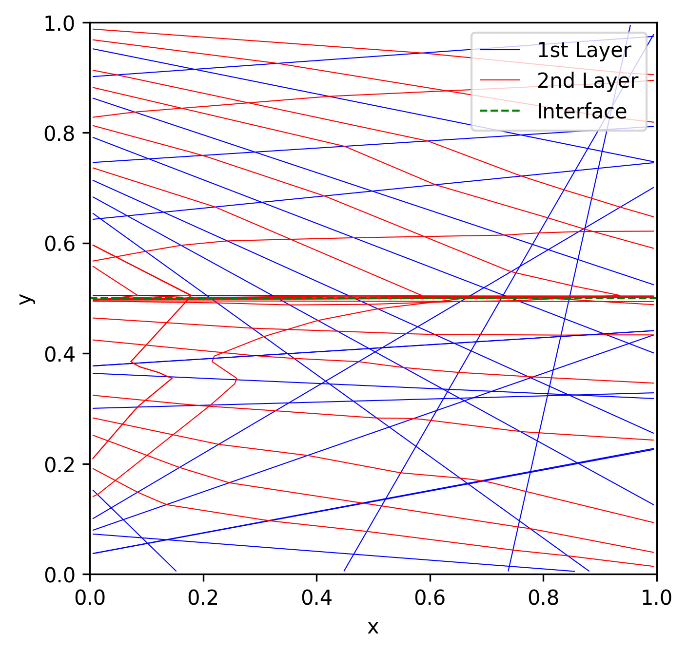
(e) The breaking hyperplanes of the approximation in Figure 7(d)

Figure 7: Approximation results of the problem in Section 4.6

Table 6: Relative errors of the problem in Section 4.6

Network structure	$\frac{\|u-{u}^{{}_{N}}_{{}_{\cal T}}\|_{0}}{\|u\|_{0}}$	$\frac{{\left|\kern-0.75346pt\left|\kern-0.75346pt\left|u-{u}^{{}_{N}}_{{}_{\cal T}}\right|\kern-0.75346pt\right|\kern-0.75346pt\right|}_{\bm{\beta}}}{{\left|\kern-0.75346pt\left|\kern-0.75346pt\left|u\right|\kern-0.75346pt\right|\kern-0.75346pt\right|}_{\bm{\beta}}}$	$\frac{\mathcal{L}^{1/2}({u}^{{}_{N}}_{{}_{\cal T}},\bf f)}{\mathcal{L}^{1/2}({u}^{{}_{N}}_{{}_{\cal T}},\bf 0)}$	Parameters
3–30–30–1	0.005082	0.027765	0.022519	1081

5 Conclusion

In this paper, we used the least-squares ReLU neural network (LSNN) method for solving linear advection-reaction equation with discontinuous solution having non-constant jumps. The method, being mesh-free, requires no mesh to resolve the interfacial discontinuity. We proved theoretically that ReLU neural network (NN) functions with $\lceil\log_{2}(d+1)\rceil+1$-layer representations are capable of approximating solutions with non-constant jumps along discontinuous interfaces that are not necessarily straight lines. Our theoretical findings were validated by multiple numerical examples with $d=2,3$ and various non-constant jumps and interface shapes, demonstrating accurate performance of the method.

The approximation of discontinuous functions by NNs is also encountered in classification tasks, and our results suggest that we can achieve accurate predictions with properly designed neural network architectures. However, in this paper, we mainly focused on the depth of NNs. The approximation of discontinuous classification functions by NNs with fixed depth and width will be addressed in a forthcoming paper.

Appendix. The proof of Theorem 3.1

In this section, we provide a proof of Theorem 3.1 by constructing a CPWL function to approximate $\chi({\bf x})$ in Eq. 9. We note that $a({\bf x})$ is generally a cylindrical surface and that the jump of $\chi({\bf x})$ is non-constant with

$$\chi(x,0)=a(x,0)=\alpha_{1}-\alpha_{2}\text{ for }x\in[0,x_{0}]$$

(see Fig. 8(a)).

(a) A cylindrical surface $a(\mathbf{x})$

(b) $(0,1)\times(y_{0},y_{0}+\varepsilon_{1})$

(c) $b(x)$ in purple and $p_{1}(x)$ in pink

Figure 8: An illustration of the convergence analysis on one subdomain $\Upsilon_{i}$

For a given $\varepsilon_{1}>0$, we take $\widehat{\Upsilon}=(0,1)\times(y_{0},y_{0}+\varepsilon_{1})$ (see Fig. 8(b)). Without loss of generality, we let $\alpha_{1}=1$, $\alpha_{2}=0$, and $\widehat{\Upsilon}=(0,1)\times(0,\varepsilon_{1})$.

Hence,

(31) $$\chi({\bf x})=\chi_{0}({\bf x})+\chi_{1}({\bf x})\text{ on }\widehat{\Upsilon},$$

where $\chi_{0}({\bf x})$ is a step function and $\chi_{1}({\bf x})$ vanishes on the inflow boundary given by

$$\chi_{0}({\bf x})=\left\{\begin{array}[]{rl}1,&{\bf x}\in\Omega_{1i}\cap\widehat{\Upsilon},\\[5.69054pt] 0,&{\bf x}\in\Omega_{2i}\cap\widehat{\Upsilon},\end{array}\right.\quad\mbox{and}\quad\chi_{1}({\bf x})=\left\{\begin{array}[]{rl}a({\bf x})-1,&{\bf x}\in\Omega_{1i}\cap\widehat{\Upsilon},\\[5.69054pt] 0,&{\bf x}\in\Omega_{2i}\cap\widehat{\Upsilon}.\end{array}\right.$$

Lemma 5.1.

Let

$$b({\bf x})=\left\{\begin{array}[]{rl}\bm{b}\cdot({\bf x}-(x_{0},0)),&{\bf x}\in\Omega_{1i}\cap\widehat{\Upsilon},\\[5.69054pt] 0,&{\bf x}\in\Omega_{2i}\cap\widehat{\Upsilon},\end{array}\right.$$

where $\bm{b}=(0,d)^{T}$ is a constant vector, and let $p_{1}({\bf x})$ be the two-layer neural network function on $\widehat{\Upsilon}$ defined by

$$p_{1}({\bf x})=-c\,\sigma({\bf w}_{1}\cdot{\bf x}+x_{0})+c\,\sigma({\bf w}_{2}\cdot{\bf x}+x_{0})$$

with the weights and coefficient

$${\bf w}_{1}=\begin{pmatrix}-1\\ -\varepsilon_{2}\end{pmatrix},\quad{\bf w}_{2}=\begin{pmatrix}-1\\ \varepsilon_{2}\end{pmatrix},\quad c=\dfrac{d}{2\varepsilon_{2}}$$

(see Fig. 8(c)). Then we have on $\widehat{\Upsilon}$,

(32) $${\left|\kern-1.07639pt\left|\kern-1.07639pt\left|b-p_{1}\right|\kern-1.07639pt\right|\kern-1.07639pt\right|}_{\bm{\beta}}=\left(\|b-p_{1}\|^{2}_{0,\widehat{\Upsilon}}+\|b_{{\bm{\beta}}}-p_{1{\bm{\beta}}}\|^{2}_{0,\widehat{\Upsilon}}\right)^{1/2}\leq\sqrt{\frac{\varepsilon_{1}^{3}}{24}+\frac{B^{2}}{4}}\,|d|\,\sqrt{\varepsilon_{1}\varepsilon_{2}},$$

where we assume $|v_{2}(\mathbf{x})|\leq B$ ($\bm{\beta}(\mathbf{x})=(0,v_{2}(\mathbf{x}))$).

Proof 5.2.

Let us denote

$$\widehat{\Upsilon}_{\varepsilon_{2}}\equiv\widehat{\Upsilon}_{1,\varepsilon_{2}}\cup\widehat{\Upsilon}_{2,\varepsilon_{2}}\equiv\{{\bf x}\in\Omega_{1i}\cap\widehat{\Upsilon}:\,{\bf w}_{1}\cdot{\bf x}+x_{0}<0\}\cup\{{\bf x}\in\Omega_{2i}\cap\widehat{\Upsilon}:\,{\bf w}_{2}\cdot{\bf x}+x_{0}>0\}.$$

Then we have

$$b({\bf x})-p_{1}({\bf x})=\left\{\begin{array}[]{rl}-c({\bf w}_{1}\cdot{\bf x}+x_{0})&{\bf x}\in\widehat{\Upsilon}_{1,\varepsilon_{2}},\\[5.69054pt] -c({\bf w}_{2}\cdot{\bf x}+x_{0})&{\bf x}\in\widehat{\Upsilon}_{2,\varepsilon_{2}},\\[5.69054pt] 0,&{\bf x}\in\widehat{\Upsilon}\setminus\widehat{\Upsilon}_{\varepsilon_{2}}.\end{array}\right.$$

Calculating the double integral,

(33) $$\|b-p_{1}\|^{2}_{0,\widehat{\Upsilon}}=\|b-p_{1}\|^{2}_{0,\widehat{\Upsilon}_{1,\varepsilon_{2}}}+\|b-p_{1}\|^{2}_{0,\widehat{\Upsilon}_{2,\varepsilon_{2}}}=\frac{d^{2}}{24}\varepsilon_{1}^{4}\varepsilon_{2},$$

and using the directional derivative,

(34) $$\|b_{{\bm{\beta}}}-p_{1{\bm{\beta}}}\|^{2}_{0,\widehat{\Upsilon}}=\int_{\widehat{\Upsilon}_{1,\varepsilon_{2}}}(c{\bf w}_{1}\cdot\bm{\beta})^{2}\,d{\bf x}+\int_{\widehat{\Upsilon}_{2,\varepsilon_{2}}}(c{\bf w}_{2}\cdot\bm{\beta})^{2}\,d{\bf x}\leq\frac{(dB)^{2}}{4}\varepsilon_{1}\varepsilon_{2}.$$

Now Eq. 32 follows from Eqs. 33 and 34.

Lemma 5.3.

Let $\widehat{\Upsilon}$, $I$, $b(\mathbf{x})$, $p_{1}(\mathbf{x})$, and $\bm{\beta}(\mathbf{x})$ be as in Lemma 5.1 with $d=\chi_{1}(0,\varepsilon_{1})/\varepsilon_{1}$, and let $p_{0}({\bf x})$ be the two-layer neural network function on $\widehat{\Upsilon}$ defined by

(35) $$p_{0}(\mathbf{x})=\frac{1}{2\varepsilon_{2}}\left(\sigma(x-x_{0}+\varepsilon_{2})-\sigma(x-x_{0}-\varepsilon_{2})\right).$$

Then we have on $\widehat{\Upsilon}$,

(36) $${\left|\kern-1.07639pt\left|\kern-1.07639pt\left|\chi-(p_{0}+p_{1})\right|\kern-1.07639pt\right|\kern-1.07639pt\right|}_{\bm{\beta}}\leq C_{1}\sqrt{\varepsilon_{1}\varepsilon_{2}}+C_{2}\sqrt{\varepsilon_{1}},$$

where $C_{2}$ is given by the square root of

(37) $$\sup\{(u_{1}(\mathbf{x})-u_{2}(\mathbf{x})-1-b(\mathbf{x}))^{2}:\mathbf{x}\in\Omega_{1i}\cap\widehat{\Upsilon}\}x_{0}\\ +\sup\{2\gamma(\mathbf{x})^{2}(u_{2}(\mathbf{x})-u_{1}(\mathbf{x}))^{2}+2(dB)^{2}:\mathbf{x}\in\Omega_{1i}\cap\widehat{\Upsilon}\}x_{0}.$$

Proof 5.4.

From the triangle inequality,

(38) $${\left|\kern-1.07639pt\left|\kern-1.07639pt\left|\chi-(p_{0}+p_{1})\right|\kern-1.07639pt\right|\kern-1.07639pt\right|}_{\bm{\beta}}={\left|\kern-1.07639pt\left|\kern-1.07639pt\left|\chi_{0}+\chi_{1}-(p_{0}+p_{1})\right|\kern-1.07639pt\right|\kern-1.07639pt\right|}_{\bm{\beta}}\leq{\left|\kern-1.07639pt\left|\kern-1.07639pt\left|\chi_{0}-p_{0}\right|\kern-1.07639pt\right|\kern-1.07639pt\right|}_{\bm{\beta}}+{\left|\kern-1.07639pt\left|\kern-1.07639pt\left|\chi_{1}-p_{1}\right|\kern-1.07639pt\right|\kern-1.07639pt\right|}_{\bm{\beta}}.$$

Since $\|\chi_{0\bm{\beta}}-p_{0\bm{\beta}}\|=0$, calculating the double integral,

(39) $$\begin{split}{\left|\kern-1.07639pt\left|\kern-1.07639pt\left|\chi_{0}-p_{0}\right|\kern-1.07639pt\right|\kern-1.07639pt\right|}_{\bm{\beta}}&=\left(\|\chi_{0}-p_{0}\|^{2}_{0,\widehat{\Upsilon}}+\|\chi_{0\bm{\beta}}-p_{0\bm{\beta}}\|^{2}_{0,\widehat{\Upsilon}}\right)^{1/2}\\ &=\|\chi_{0}-p_{0}\|_{0,\widehat{\Upsilon}}\\ &=\frac{1}{\sqrt{6}}\,\sqrt{\varepsilon_{1}\varepsilon_{2}}.\end{split}$$

Next, again, by the triangle inequality,

$${\left|\kern-1.07639pt\left|\kern-1.07639pt\left|\chi_{1}-p_{1}\right|\kern-1.07639pt\right|\kern-1.07639pt\right|}_{\bm{\beta}}\leq{\left|\kern-1.07639pt\left|\kern-1.07639pt\left|\chi_{1}-b\right|\kern-1.07639pt\right|\kern-1.07639pt\right|}_{\bm{\beta}}+{\left|\kern-1.07639pt\left|\kern-1.07639pt\left|b-p_{1}\right|\kern-1.07639pt\right|\kern-1.07639pt\right|}_{\bm{\beta}}.$$

By Lemma 5.1

$${\left|\kern-1.07639pt\left|\kern-1.07639pt\left|b-p_{1}\right|\kern-1.07639pt\right|\kern-1.07639pt\right|}_{\bm{\beta}}\leq\sqrt{\frac{\varepsilon_{1}^{3}}{24}+\frac{B^{2}}{4}}\,|d|\,\sqrt{\varepsilon_{1}\varepsilon_{2}}.$$

To bound ${\left|\kern-1.07639pt\left|\kern-1.07639pt\left|\chi_{1}-b\right|\kern-1.07639pt\right|\kern-1.07639pt\right|}_{\bm{\beta}}$, we recall the definition of the graph norm,

$${\left|\kern-1.07639pt\left|\kern-1.07639pt\left|\chi_{1}-b\right|\kern-1.07639pt\right|\kern-1.07639pt\right|}_{\bm{\beta}}=\left(\|\chi_{1}-b\|^{2}_{0,\widehat{\Upsilon}}+\|\chi_{1\bm{\beta}}-b_{\bm{\beta}}\|^{2}_{0,\widehat{\Upsilon}}\right)^{1/2}.$$

First we have

$$\begin{split}\|\chi_{1}-b\|^{2}_{0,\widehat{\Upsilon}}&=\|\chi_{1}-b\|^{2}_{0,\Omega_{1i}\cap\widehat{\Upsilon}}\\ &\leq\sup\{(\chi_{1}(\mathbf{x})-b(\mathbf{x}))^{2}:\mathbf{x}\in\Omega_{1i}\cap\widehat{\Upsilon}\}\varepsilon_{1}x_{0}\\ &=\sup\{(u_{1}(\mathbf{x})-u_{2}(\mathbf{x})-1-b(\mathbf{x}))^{2}:\mathbf{x}\in\Omega_{1i}\cap\widehat{\Upsilon}\}\varepsilon_{1}x_{0}.\end{split}$$

Next, observing $b_{\bm{\beta}}=dv_{2}$ and from Eq. 2,

$$\chi_{1\bm{\beta}}=(u_{1}-u_{2}-1)_{\bm{\beta}}=(u_{1}-u_{2})_{\bm{\beta}}=\gamma(u_{2}-u_{1}),$$

we have

$$\begin{split}\|\chi_{1\bm{\beta}}-b_{\bm{\beta}}\|^{2}_{0,\widehat{\Upsilon}}&=\|\chi_{1\bm{\beta}}-b_{\bm{\beta}}\|^{2}_{0,\Omega_{1i}\cap\widehat{\Upsilon}}\\ &=\|\gamma(u_{2}-u_{1})-dv_{2}\|^{2}_{0,\Omega_{1i}\cap\widehat{\Upsilon}}\\ &\leq\left\lVert\sqrt{2\gamma^{2}(u_{2}-u_{1})^{2}+2(dv_{2})^{2}}\right\rVert^{2}_{0,\Omega_{1i}\cap\widehat{\Upsilon}}\\ &\leq\sup\{2\gamma(\mathbf{x})^{2}(u_{2}(\mathbf{x})-u_{1}(\mathbf{x}))^{2}+2(dB)^{2}:\mathbf{x}\in\Omega_{1i}\cap\widehat{\Upsilon}\}\varepsilon_{1}x_{0}.\end{split}$$

Now Eq. 36 follows from combining the above inequalities.

Given $\varepsilon_{3}>0$, let us choose $\varepsilon_{1}=1/m$ such that

(40) $$\sup\{(u_{1}({\bf x})-u_{2}({\bf x})-\chi(0,j/m)-b_{j}(\mathbf{x}))^{2}:\mathbf{x}\in\Omega_{1i}\cap\widehat{\Upsilon}_{j}\},\\ \sup\{2\gamma(\mathbf{x})^{2}(u_{2}(\mathbf{x})-u_{1}(\mathbf{x}))^{2}+2(d_{j}B)^{2}:\mathbf{x}\in\Omega_{1i}\cap\widehat{\Upsilon}_{j}\}<\varepsilon_{3},$$

where $\widehat{\Upsilon}_{j}=(0,1)\times(j/m,(j+1)/m)$ for $j=0,\ldots,m-1$, and $b_{j}(\mathbf{x})$ and $d_{j}$ are as in Lemma 5.3. Then we define on each $\widehat{\Upsilon}_{j}$, $p_{0j}(\mathbf{x}),p_{1j}(\mathbf{x})$ as in Lemma 5.3, and construct the CPWL function $p_{i}(\mathbf{x})$ on $\Upsilon_{i}$ defined by

$$p_{i}(\mathbf{x})=p_{0j}(\mathbf{x})+p_{1j}(\mathbf{x}),\ \mathbf{x}\in\widehat{\Upsilon}_{j}.$$

Proof 5.5 (Proof of Theorem 3.1).

By Lemma 5.3 and the given condition,

(41) $$\begin{split}{\left|\kern-1.07639pt\left|\kern-1.07639pt\left|\chi-p_{i}\right|\kern-1.07639pt\right|\kern-1.07639pt\right|}_{\bm{\beta}}&=\left(\sum_{j=0}^{m-1}{\left|\kern-1.07639pt\left|\kern-1.07639pt\left|\chi-(p_{0j}+p_{1j})\right|\kern-1.07639pt\right|\kern-1.07639pt\right|}^{2}_{\bm{\beta}}\right)^{1/2}\\ &\leq\left(\sum_{j=0}^{m-1}\left(D_{1j}\sqrt{\varepsilon_{1}\varepsilon_{2}}+D_{2j}\sqrt{\varepsilon_{1}\varepsilon_{3}}\right)^{2}\right)^{1/2}\\ &\leq\left(m\max_{0\leq j\leq m-1}\left(D_{1j}\sqrt{\varepsilon_{1}\varepsilon_{2}}+D_{2j}\sqrt{\varepsilon_{1}\varepsilon_{3}}\right)^{2}\right)^{1/2}\\ &=\sqrt{m}\max_{0\leq j\leq m-1}\left(D_{1j}\sqrt{\varepsilon_{1}\varepsilon_{2}}+D_{2j}\sqrt{\varepsilon_{1}\varepsilon_{3}}\right)\\ &=\max_{0\leq j\leq m-1}\left(D_{1j}\sqrt{\varepsilon_{2}}+D_{2j}\sqrt{\varepsilon_{3}}\right),\end{split}$$

where for the first identity, each norm on the right-hand side is taken over $\widehat{\Upsilon}_{j}$. Now $D_{1}=D_{1k}$ and $D_{2}=D_{2k}$ for some $0\leq k\leq m-1$.

References

[1]R. Arora, A. Basu, P. Mianjy, and A. Mukherjee, Understanding deep
neural networks with rectified linear units, arXiv preprint
arXiv:1611.01491, (2016), https://doi.org/10.48550/arXiv.1611.01491.
[2]P. Bochev and J. Choi, Improved least-squares error estimates for
scalar hyperbolic problems, Comput. Methods Appl. Math., 1 (2001),
pp. 115–124, https://doi.org/10.2478/cmam-2001-0008.
[3]Z. Cai, J. Chen, and M. Liu, Least-squares neural network (LSNN)
method for scalar nonlinear hyperbolic conservation laws: discrete divergence
operator, J. Comput. Appl. Math. 433 (2023) 115298,
https://doi.org/10.48550/arXiv.2110.10895.
[4]Z. Cai, J. Chen, and M. Liu, Least-squares ReLU neural network
(LSNN) method for linear advection-reaction equation, J. Comput. Phys. 443
(2021) 110514, https://doi.org/10.1016/j.jcp.2021.110514.
[5]Z. Cai, J. Choi, and M. Liu, Least-squares neural network (lsnn)
method for linear advection-reaction equation: General discontinuous
interface, arXiv preprint arXiv:2301.06156, (2023),
https://doi.org/10.48550/arXiv.2301.06156.
[6]W. Dahmen, C. Huang, C. Schwab, and G. Welper, Adaptive
petrov–galerkin methods for first order transport equations, SIAM J. Numer.
Anal., 50 (2012), pp. 2420–2445, https://doi.org/10.1137/110823158.
[7]H. De Sterck, T. A. Manteuffel, S. F. McCormick, and L. Olson, Least-squares finite element methods and algebraic multigrid solvers for
linear hyperbolic PDEs, SIAM J. Sci. Comput., 26 (2004), pp. 31–54,
https://doi.org/10.1137/S106482750240858X.
[8]P. Houston, R. Rannacher, and E. Süli, A posteriori error
analysis for stabilised finite element approximations of transport problems,
Comput. Methods Appl. Mech. Engrg., 190 (2000), pp. 1483–1508,
https://doi.org/10.1016/S0045-7825(00)00174-2.
[9]D. P. Kingma and J. Ba, ADAM: A method for stochastic
optimization, in International Conference on Representation Learning, San
Diego, 2015.
[10]M. Leshno, V. Y. Lin, A. Pinkus, and S. Schocken, Multilayer
feedforward networks with a nonpolynomial activation function can approximate
any function, Neural networks, 6 (1993), pp. 861–867.
[11]Q. Liu and S. Zhang, Adaptive least-squares finite element methods
for linear transport equations based on an H(div) flux reformulation,
Comput. Methods Appl. Mech. Engrg., (366 (2020) 113041),
https://doi.org/10.1016/j.cma.2020.113041.