Ultra-efficient MCMC for Bayesian longitudinal functional data analysis
Abstract
Functional mixed models are widely useful for regression analysis with dependent functional data, including longitudinal functional data with scalar predictors. However, existing algorithms for Bayesian inference with these models only provide either scalable computing or accurate approximations to the posterior distribution, but not both. We introduce a new MCMC sampling strategy for highly efficient and fully Bayesian regression with longitudinal functional data. Using a novel blocking structure paired with an orthogonalized basis reparametrization, our algorithm jointly samples the fixed effects regression functions together with all subject- and replicate-specific random effects functions. Crucially, the joint sampler optimizes sampling efficiency for these key parameters while preserving computational scalability. Perhaps surprisingly, our new MCMC sampling algorithm even surpasses state-of-the-art algorithms for frequentist estimation and variational Bayes approximations for functional mixed models—while also providing accurate posterior uncertainty quantification—and is orders of magnitude faster than existing Gibbs samplers. Simulation studies show improved point estimation and interval coverage in nearly all simulation settings over competing approaches. We apply our method to a large physical activity dataset to study how various demographic and health factors associate with intraday activity.
Keywords: Actigraphy data, Function-on-scalar regression, Gibbs sampler, Mixed models
1 Introduction
Functional data analysis (FDA) refers to the statistical analysis of data objects observed over a continuum, such as time or space, typically at high resolutions. FDA has been applied in a variety of important areas, including climate data (Besse et al., 2000), electricity prices (Liebl, 2013), COVID-19 dynamics (Boschi et al., 2021), and many others. FDA is particularly challenging when the functional data are dependent, which requires more sophisticated statistical models and more intensive computations. We focus on regression analysis with longitudinal functional data, which presents the simultaneous challenges of (i) within-curve dependencies, (ii) groupings among repeated (functional) measurements, and (iii) associations with (possibly many) scalar covariates.
To meet these challenges, functional mixed models (FMMs) have emerged as a powerful modeling tool. FMMs combine FDA and traditional mixed effects models to provide regression analysis of functional data in the presence of structured dependence. However, longitudinal functional datasets are often massive, with millions or billions of high-resolution measurements (Doherty et al., 2017; Lee et al., 2019). Thus, recent work has increasingly prioritized the computational scalability of FMMs. Naturally, the attendant computational burdens are exacerbated by the complexity of the statistical model, including various covariance structures and (possibly many) scalar covariates. As a result, there is high demand for inferential algorithms for FMMs that both (i) scale to massive datasets and (ii) maintain these essential modeling capabilities.
These challenges are exemplified in our motivating application, the 2005-2006 National Health and Nutrition Examination Survey (NHANES) physical activity (PA) dataset. High resolution (minute-by-minute) PA data (Figure 1) are recorded across multiple days for each participant using hip-worn accelerometry devices and linked to a questionnaire that contains subject-level demographic and health information (Table 2). Figure 1 shows the PA levels of two randomly chosen subjects for every day they wore the device. Key aspects of the data become evident from this plot: the observations are high-resolution, noisy, autocorrelated, and exhibit considerable variation both between subjects and between days for a given subject. Notably, there are more than 72 million PA measurements on more than 10,000 participants in the study (Leroux et al., 2019). The goal is to link time-of-day PA with important health and demographic variables, while appropriately accounting for the prominent and complex dependencies among these high-dimensional data.
To enable statistical modeling and inference, we represent the PA as longitudinal functional data: the PA measurements are functions of time-of-day and the days are repeated measurements of these functional data for each subject. More generally, let denote functional observations on a compact domain (i.e., time-of-day) for within-subject replications (i.e., days) and subjects , with . The functional data are linked to scalar covariates for subject and replicate . We study the following FMM for longitudinal functional regression:
| (1) |
Model (1) extends traditional mixed effects models for longitudinal data to the functional data setting by allowing the fixed effects and the random effects to vary as functions of . First, the fixed effects are regression coefficient functions and describe the linear associations between and at each . Next, the random effects are shared among all functional observations for subject , and thus account for subject-specific effects and dependencies among repeated (functional) observations. The replicate-specific random effects account for within-curve dependencies (or “smooth” errors) that are unexplained by the fixed effects or subject-specific random effects. These effects are especially important for functional regression, even without repeated measurements (Reiss et al., 2010; Kowal and Bourgeois, 2020). Finally, the errors describe any (non-smooth) measurement errors that remain. The random effects functions and errors are mean zero and mutually independent, with additional modeling assumptions discussed subsequently.
The FMM (1) is widely applicable and has appeared in many previous studies (Zipunnikov et al., 2014; Cederbaum et al., 2016; Zhu et al., 2019; Li et al., 2022), including both special cases without replications (; Guo, 2002) or covariates (Park and Staicu, 2015) as well as generalizations for additive (Scheipl et al., 2015) or non-Gaussian responses (Scheipl et al., 2016). However, computational considerations are paramount, and often preclude the use of these generalized models even for moderately-sized datasets (Sergazinov et al., 2023). In response, Cui et al. (2022) proposed Fast Univariate Inference (FUI) for (1), which seeks to dramatically simplify estimation by (i) fitting separate linear mixed models pointwise for each , (ii) applying a smoother to the estimated pointwise fixed effects, and (iii) using asymptotic arguments or bootstrapping to obtain confidence bands for . Such a deconstruction sacrifices estimation efficiency and is difficult to apply for sparsely- or irregularly-sampled functional data. Like other frequentist approaches, FUI requires selection of tuning (smoothing) parameters and provides limited uncertainty quantification for certain parameters and predictions. Yet most important, we show subsequently that such a decomposition is not necessary to achieve scalable computing—and in fact that FUI is slower than our fully Bayesian approach (see Section 4).
In general, Bayesian approaches for FMMs are highly appealing due to the consolidated interpretation of fixed and random effects, as well as convenient uncertainty quantification of all model parameters and predictions. Morris and Carroll (2006) introduced Bayesian FMMs using a wavelet basis expansion for fixed and random effects. This approach has been extended and applied broadly (Zhu et al., 2011; Morris, 2017; Lee et al., 2019), but leverages unique features of the wavelet basis—which may not be suitable for smoother functional data and is difficult to apply when the number of functional observations is non-dyadic—and requires Metropolis-Hastings sampling steps for all variance components. Bayesian FMMs commonly rely on Markov chain Monte Carlo (MCMC) sampling for posterior inference, typically using Gibbs sampling (Morris and Carroll, 2006; Goldsmith and Kitago, 2016; Lee et al., 2019) or Hamiltonian Monte Carlo (Goldsmith et al., 2015). Advantageously, these algorithms provide exact (up to Monte Carlo error) inference, but are prohibitively slow, with running times in the hours or days even for moderately-sized datasets (see Section 4). Further, certain MCMC sampling strategies are vulnerable to slow mixing and convergence: for example, Goldsmith and Kitago (2016) applied a Gibbs sampler that alternates sampling blocks for the fixed effects and the random effects, which is sensitive to the model parameterization (i.e., centered vs. noncentered; Yu and Meng, 2011) and can lead to poor exploration of the joint target distribution. Our analyses confirm the MCMC inefficiencies of this blocking strategy, which compounds the impact of the extremely lengthy computing times.
To reduce this computational burden, there has been recent development for variational Bayes (VB) approximations for Bayesian FMMs. VB substantially reduces computation times compared to existing MCMC algorithms (Goldsmith and Kitago, 2016; Huo et al., 2022). However, VB often provides poor uncertainty quantification, and thus Goldsmith and Kitago (2016) recommend it primarily as a tool to obtain quick initial estimates for model-building. Our simulations (Section 4) show that VB is adequate for point estimation, but falls considerably short in interval estimation. Thus, there is urgent demand for algorithms that can provide both accurate and scalable Bayesian inference for the FMM (1).
We address this significant gap in the literature. Specifically, we design an MCMC sampling algorithm for the FMM (1) that offers several unique features. First, we jointly sample all fixed and random effects functions , which delivers superior Monte Carlo efficiency for these critical quantities. Second, we design this joint sampler using a careful blocking structure paired with an orthogonalized basis reparametrization, which leads to exceptionally fast sampling steps. The accompanying variance components are sampled in a separate block, yielding a convenient Gibbs sampler that is both computationally and Monte Carlo efficient. Perhaps surprisingly, our new MCMC sampling algorithm even surpasses state-of-the-art algorithms for frequentist estimation (Cui et al., 2022; Li et al., 2022) and VB approximations (Goldsmith and Kitago, 2016) and is orders of magnitude faster than existing Gibbs samplers for FMMs. This superior scaling persists across number of subjects , number of replicates per subject, and number of covariates , and is accompanied by more accurate point estimation and uncertainty quantification across nearly all tested scenarios. Applying our methods to the NHANES PA dataset, we demonstrate the significant practical impacts of our improved MCMC algorithm and provide posterior uncertainty quantification for key parameters. Compared to existing MCMC algorithms, we reduce the computation time from two weeks to only a few minutes.
The rest of this article is organized as follows. Section 2 presents the Bayesian FMM for longitudinal data. Section 3 describes the MCMC algorithm. Section 4 provides simulation analyses. We apply our model on the NHANES dataset in Section 5. We conclude with a discussion in Section 6. R code to implement our approach and replicate our results is available at https://github.com/thomasysun/FLFOSR.
2 Basis expansions and prior distributions
FMMs (1) are most commonly implemented using basis expansions, including splines (Guo, 2002; Goldsmith and Kitago, 2016), functional principal components (Park and Staicu, 2015; Li et al., 2022), and wavelets (Morris and Carroll, 2006; Huo et al., 2022). The general basis representation of (1) is
| (2) | ||||
| (3) |
where are known basis functions and are unknown basis coefficients. Model (2)–(3) induces (1) under the identification and similarly for the remaining fixed and random effects functions. The coefficients are completely determined by , and merely serve as a placeholder for notational convenience. Because the basis functions are known, estimation and inference for the coefficients is sufficient for estimation and inference of the functions .
The choice of basis functions must be paired carefully with the choice of prior on the coefficients , which together induce a prior for functions . Typically, we select the prior on the coefficients to encourage certain properties for the functions, such as smoothness (Goldsmith et al., 2015; Goldsmith and Kitago, 2016; Kowal and Bourgeois, 2020) or sparsity (Morris and Carroll, 2006). Here, we also prioritize the resulting computational implications.
To motivate the general approach, suppose that we are interested in specifying a prior for a generic function under a basis expansion:
A common strategy is to assume a prior of the form
where is a known (roughness) penalty matrix and is a (smoothness) parameter. For instance, suppose is the matrix of integrated squared second derivatives, , where denotes the second derivative of . Then the prior for may be expressed as
and denotes equality up to an additive constant. Thus, the log-prior on reproduces the classical roughness penalty on the function . In a Bayesian framework, we further may place a prior on to learn the smoothness parameter; these details are discussed below in the context of model (2)–(3).
Although this approach is advantageous due to its generality and smoothness-inducing properties, it is unfavorable for computing, especially within the basis-expanded FMM (2)–(3). Suppose we observe data at and let be the basis matrix with . For a generic basis , there is no special structure for or . Thus, we seek to reparamaterize these terms —at a one-time cost for all subsequent MCMC sampling—for more amenable computing. Specifically, we apply the orthogonalization strategy from Scheipl et al. (2012), which uses the spectral decomposition of to form a basis matrix such that (i) is a diagonal matrix and (ii) has the same distribution as , where . Notably, this strategy applies for any basis and penalty matrix ; in our empirical examples, we use B-splines with a penalty on the second differences of the coefficients.
Revisiting the FMM basis expansion (2)–(3), we henceforth assume, without loss of generality, that is diagonal and that arbitrary (roughness) penalties may be incorporated via independent Gaussian priors. Thus, we specify the priors
| (4) |
and assume that the reparametrization has already been completed. In conjunction with the basis expansions, the priors (4) induce a Gaussian process prior for each fixed and random effect function, e.g.,
and similarly for the remaining terms.
Finally, we assume conditionally conjugate Gamma priors for the precision parameters,
| (5) |
along with a Jeffreys’ prior for the observation error variance, . These parameters determine both the smoothness of the corresponding functions as well as the various sources of variability within a function, between replicates for a subject, and between subjects. Other priors are available for variance parameters (Gelman, 2006), and may be substituted into the proposed framework with minimal impact on the core MCMC sampling approach. However, we find that (5) offers excellent modeling performance and MCMC efficiency, and is not highly sensitive to the choice of (see the supplementary material for a sensitivity analysis).
In practice, we observe the functional data at discrete points . For simplicity, we assume that these observation points are common for all , but it is straightforward to accommodate sparsely- or irregularly-sampled functional data within a Bayesian framework (Kowal et al., 2019). The likelihood under (2) with observed data is
| (6) |
We emphasize that the modeling choices in (2)–(5) are meant to be broadly applicable—including generic basis expansions, penalty matrices, and variance components (or smoothness parameters) for each fixed and random effects function. The main contributions of this paper are not found in the uniqueness of this modeling strategy, but rather in our MCMC sampling algorithm for the general Bayesian FMM (1), which is presented in the next section. The essential features of our FMM specification are (i) the basis expansions (2) and (ii) the conditionally Gaussian priors (4), in conjunction with the aforementioned basis orthogonalization strategy (Scheipl et al., 2012).
3 MCMC Algorithm
The primary challenge is to construct a sampling algorithm for the joint posterior distribution of the fixed and random effects functions under the FMM (1). This task requires simultaneous consideration of (i) MCMC efficiency, including convergence and autocorrelation of the Markov chain, and (ii) computational scalability across all dimensions of the data: the number of subjects , the number of replicates per subject, number of covariates , and the number of observation points along each curve. We focus on the sampling steps for the fixed and random effects basis coefficients , which are sufficient for posterior inference for the fixed and random effects functions under (2)–(3). The variance components are sampled in a separate block, resulting in a two-block Gibbs sampling algorithm (Algorithm 1).
We propose a joint sampler for all fixed and random effects functions by carefully decomposing the joint posterior distribution of the corresponding basis coefficients. First, let , , and , where , and let and similarly for and . Similarly, define the diagonal variance matrices , , , and , where the set of variances are first iterated through for and so on to yield terms along the diagonal. Let contain all variance components.
The joint fixed and random effects posterior (conditional on ) is decomposable as
| (7) |
where denotes all observed data. Our Gibbs sampler iterates between joint sampling blocks from (7) and ; the latter sampling step is straightforward (see Algorithm 1), so we focus on (7).
We sample from the joint posterior (7) by iteratively drawing from the three constituent terms: (i) the marginal posterior of the fixed effects , (ii) the partial conditional posterior of the subject-specific random effects given the fixed effects , and (iii) the full conditional posterior of the replicate-specific random effects . In contrast to a Gibbs sampler that draws from the three full conditional distributions , , and (e.g., Goldsmith and Kitago, 2016), our approach delivers a direct Monte Carlo (not MCMC) sample from the joint posterior (conditional on ), and thus offers the potential for large gains in sampling efficiency (see Figure 2). Further, the joint sampler requires no consideration of centered versus non-centered parameterizations of the mixed effects model, which eliminates a recurring nuisance for Bayesian implementations of mixed and hierarchical models (Yu and Meng, 2011). However, we must also carefully consider the resulting computational burden of these sampling steps. In particular, a sampling algorithm that offers Monte Carlo efficiency may nonetheless be infeasible in practice, if the raw computing times scale poorly in , , , or .
Our key innovation is that we provide convenient, closed-form, and highly scalable sampling steps for the constituent distributions in (7). First, observe that in (2)–(3) contains all fixed and random effects coefficients, and thus may be viewed as a placeholder for each of the random variables in (7). Since the reparametrized basis matrix satisfies , the joint likelihood (6) for may be written
| (8) | ||||
| (9) |
up to constants that do not depend on , where the coefficients are computed by projecting the functional observations onto the basis matrix, . Thus, the only dependence on is via this projection step, which is a one-time cost for all subsequent MCMC sampling. In addition, the joint posterior factorizes across the basis coefficients,
and we may sample the fixed and random effects coefficients separately for each . This strategy is parallelizable across yet still maintains a joint sampler for all fixed and random effects coefficients. This offers a substantial simplification from the functional data likelihood in (8), which features -dimensional terms , especially since in general. Finally, the likelihood (9) for is proportional to the likelihood for implied by the simple working model
| (10) | ||||
| (11) |
It is typically easier to derive the posterior distributions for in (7) using (10)–(11) instead of (6) or (8), yet the results are equivalent.
We describe the three sampling steps in ascending complexity, which reverses the actual sampling order from (7). Let denote the projected functional data ordered by replicates for each subject, be the design matrix with a column of ones for the intercept, and , a block diagonal matrix with columns and -dimensional vectors of ones.
The simplest sampling step is the full conditional distribution for the replicate-specific coefficients:
| (12) |
for . Most important, the posterior precision matrix is diagonal, and thus all the replicate-specific coefficients may be sampled independently (and in parallel) in computing time.
Next, we provide the sampling step for the partial conditional of the subject-specific random effects, , which marginalizes over . Under the prior (4), it is easy to see that the marginalized version of (11) is simply , where . The requisite distribution is then
| (13) |
where for . Crucially, the posterior precision matrix is diagonal, and thus all subject-specific coefficients may be sampled independently (and in parallel) in computing time.
While the posterior precision matrices for and are diagonal and easy to construct, we must also consider computation of the vectors and . An important observation is that, for arbitrary matrix , the operations (or ) repeat row (or column ) of times, while (or ) sums over the columns (or rows) for all rows (or columns) corresponding to the same subject . The matrix notation obscures the simplicity of these computations, which are vectorizable and thus offer additional efficiency gains in R.
The remaining sampling step is the marginal posterior of the fixed effects, , which requires marginalization over all random effects coefficients . Once more, the working model (10)–(11) is particularly convenient for these derivations, and yields the distribution
| (14) |
where and for . Unlike for the random effects coefficients, the posterior precision for is not diagonal; indeed, is the only non-diagonal posterior precision matrix in our joint sampler for all . To alleviate this potential bottleneck when the number of covariates is large, we apply the sampling algorithm from Rue (2001) when and the sampling algorithm from Bhattacharya et al. (2016) when . This sampling strategy has been successful in (non-longitudinal) function-on-scalars regression (Kowal and Bourgeois, 2020). More generally, (14) has the same structure as in (non-functional) Bayesian linear regression models, and thus we may adapt and apply new sampling strategies for that setting as the state-of-the-art advances (Nishimura and Suchard, 2022).
In aggregate, we present our full MCMC sampling algorithm in Algorithm 1. The joint sampling step for is highly scalable, and in fact delivers the same computational cost as a naive Gibbs sampler that instead use the three full conditional draws , , and —while offering the potential for substantial increases in MCMC efficiency.
From a practical perspective, we emphasize that many computations are parallelizable, including the sampling steps for all , while many constituent terms are highly vectorizable. For instance, and are diagonal, and computing simply consists of multiplying each row of the matrix by the corresponding scalar value . Within R, we maximize computational performance by avoiding matrix calculations wherever possible and opting for vectorized operations instead. This is in contrast to common FMM formulations that utilize matrix operations with Kronecker products or large block matrices, and thus face significant computational bottlenecks.
Lastly, we reiterate that Algorithm 1 is applicable for any Bayesian FMM that satisfies a basis expansion (2)–(3) and assumes (conditionally) Gaussian priors (4). Thus, our approach is broadly applicable for many choices of basis functions, and remains valid for generic smoothness priors using the basis orthogonalization strategy of Scheipl et al. (2012). We henceforth refer to our approach as fast longitudinal function-on-scalar regression (FLFOSR).
4 Simulations
We conduct a series of simulation studies to evaluate the performance of our approach against state-of-the-art Bayesian and frequentist competitors. Specifically, we assess (i) the MCMC efficiency and computational costs and (ii) the estimation accuracy and uncertainty quantification under various simulation designs.
4.1 Simulation Design
Functional observations are generated from the FMM (1) using the basis representation (2)–(3). We fix and simulate the coefficients , , and independently, and then compute . The variance components are varied in Sections 4.3 and 4.4 to evaluate performance under different sources of variability. Finally, functional data are generated from (2), where the basis functions are orthogonalized B-spline basis functions and is a grid of equally-spaced points in , which emulates the PA data in Section 5. We emphasize that although this data-generating process resembles the proposed Bayesian FMM, the same model structure is shared among all competing methods, and thus does not unfairly favor our approach.
4.2 Competing methods
We compare the proposed FLFOSR approach against several Bayesian and frequentist methods for regression analysis with longitudinal functional data. The Bayesian competitors come from the widely-used refund package in R (Goldsmith et al., 2021), and feature both the Gibbs sampler (refund:Gibbs) and the VB approximation (refund:VB) from Goldsmith and Kitago (2016). Unlike FLFOSR, refund:Gibbs (i) uses the full conditional draws for all fixed and random effects instead of the joint sampler (Algorithm 1), (ii) does not orthogonalize the basis functions, and (iii) sets the hyperparameters of the variance components based on an initial estimate of the residual covariance matrix. We expect that (i) will inhibit MCMC efficiency and (ii) will decrease computational scalability.
Among frequentist approaches, there is a rich collection of recent strategies and software. We focus on FUI (Cui et al., 2022), which specifically advertises computational scalability for longitudinal function-on-scalar regression, and Li et al. (2022), which provides fixed effects inference for a variety of longitudinal correlation structures. We choose to work with the exchangeable correlation model since this mirrors our model assumptions. More general methods for FMMs or functional additive mixed models could be considered for this problem. However, the widely-used implementations (i.e., pffr in the refund package) are known to have severe bottlenecks for both computing and memory (Cui et al., 2022; Sergazinov et al., 2023). Thus, such methods were not included in the study.
For FLFOSR, we set the hyperparameters to be and assess sensitivity in the supplementary material. All methods used basis functions. Any remaining settings were fixed at the default choices in the provided R functions. Simulations were performed on a Windows desktop with a 3.60 GHz Intel Xeon CPU with 32 GB of RAM.
4.3 Evaluating MCMC efficiency and computational scalability
Among Bayesian methods, we measure MCMC efficiency using effective sample sizes (ESS), which equivalently summarize the autocorrelation in the Markov chain (Gelman et al., 2013). For each MCMC sampler, we generate draws from a single chain after discarding the initial draws as burn-in, and then compute the pointwise ESS of each fixed effect regression coefficient function for and . We also record and , the total running times (in seconds) to obtain and draws, respectively.
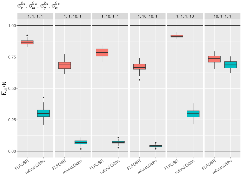
First, we compute the average relative efficiency across all covariates and observation points,
which exclusively measures MCMC efficiency (not computing time). We compare this metric between the competing MCMC samplers, FLFOSR and refund:Gibbs, using the simulation design from Section 4.1. Figure 2 presents results across various settings for the variance components and , , and (a smaller dataset is necessary for refund:Gibbs; see Figure 3). FLFOSR is dramatically more efficient than refund:Gibbs, with consistently excellent performance across all setting. By comparison, the MCMC efficiency of refund:Gibbs deteriorates significantly whenever or is large. This result is unsurprising: for Gibbs samplers that alternate between drawing the fixed and the random effects from their respective full conditional distributions (e.g., refund:Gibbs), it is well-known that the model parameterization (centered vs. noncentered) is critical for MCMC efficiency (Yu and Meng, 2011). In particular, the performance depends on the relative magnitudes of the variance components, which in practice are unknown. By comparison, FLFOSR samples the fixed and random effects functions jointly, and thus requires no consideration of the parametrization—and achieves excellent MCMC efficiency across a variety of settings.
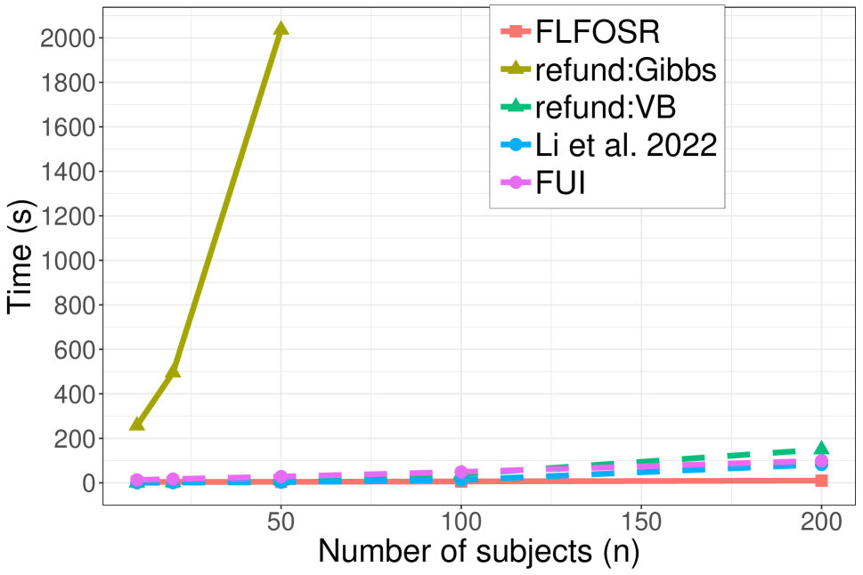
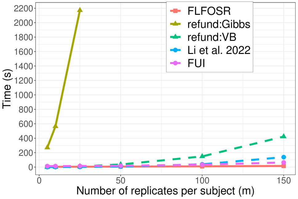
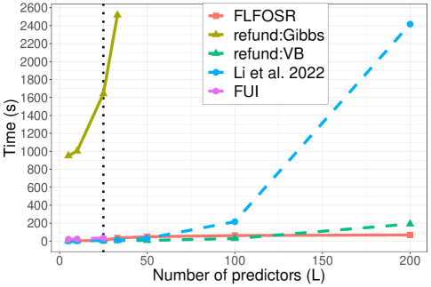
Next, we summarize aggregate computational performance by measuring the time needed to generate effective samples, averaged over all covariates and observation points,
which rewards both MCMC efficiency and computational scalability. This quantity allows some comparison between Bayesian and frequentist algorithms: although an MCMC algorithm may be run arbitrarily long to secure greater accuracy, 1000 effective samples is a reasonable and conservative target for general sampling-based inference.
Using the simulation design from Section 4.1, we scale the size of simulated datasets across three separate dimensions: (i) the number of subjects , fixing and ; (ii) the number of replicates or repeated observations per subjects, , fixing and ; and (iii) the number of predictors , fixing and . Data were generated using , and . The computing times for each algorithm are averaged across 30 datasets in each simulation setting.
The computational performance of each method is summarized in Figure 3 and detailed further in Table 1. Once again, FLFOSR decisively outperforms the MCMC competitor (refund:Gibbs): FLFOSR delivers more efficient exploration of the posterior while reducing computational costs by several orders of magnitude. These results highlight the mutual importance of (i) the joint sampling step for and (ii) the careful construction of fast constituent sampling steps (Algorithm 1). For instance, FLFOSR generates 1000 average effective samples in under 10 seconds for a dataset with 144,000 data points (, , ). By comparison, refund:Gibbs requires several minutes for only subjects, and is not feasible even for moderately-sized datasets.
Yet most surprisingly, FLFOSR attains 1000 effective samples in less time than it takes for either the VB approximation or state-of-the-art frequentist algorithms (Li et al., 2022; Cui et al., 2022) to terminate. These computing gains accelerate as each dimension , , or increases. Further, FUI scales poorly in and requires , while FLFOSR has no such restrictions. These results were obtained from a single machine without utilizing any parallel processing. Thus, further scalability is attainable for FLFOSR.
| FLFOSR | refund:Gibbs | refund:VB | Li et al. | FUI | |||||
| 10 | 5 | 5 | 4.5 | 0.59 | 257.1 | 0.57 | 0.7 | 0.4 | 12.9 |
| 20 | 5 | 5 | 4 | 0.73 | 495.5 | 0.71 | 2 | 0.8 | 16.9 |
| 50 | 5 | 5 | 4.5 | 0.86 | 2036.4 | 0.79 | 9.6 | 2.9 | 28.1 |
| 100 | 5 | 5 | 6.3 | 0.88 | - | - | 38.8 | 13.1 | 49.1 |
| 200 | 5 | 5 | 9.9 | 0.9 | - | - | 149.9 | 82.6 | 99.6 |
| 10 | 5 | 5 | 4.7 | 0.59 | 270 | 0.57 | 0.8 | 0.5 | 13.8 |
| 10 | 10 | 5 | 4.5 | 0.65 | 564 | 0.65 | 2 | 0.7 | 13.9 |
| 10 | 25 | 5 | 5.2 | 0.73 | 2171.4 | 0.76 | 9.7 | 2 | 15.3 |
| 10 | 50 | 5 | 6.9 | 0.75 | - | - | 36.3 | 7.2 | 19 |
| 10 | 100 | 5 | 10.5 | 0.79 | - | - | 147.9 | 38.9 | 33.1 |
| 10 | 150 | 5 | 16 | 0.79 | - | - | 422.7 | 137.9 | 64.2 |
| 30 | 5 | 5 | 4 | 0.81 | 950.2 | 0.75 | 3.9 | 1.2 | 20.3 |
| 30 | 5 | 10 | 4.3 | 0.77 | 1002.5 | 0.74 | 4 | 1.9 | 23.5 |
| 30 | 5 | 25 | 6.1 | 0.63 | 1641.1 | 0.62 | 4.6 | 5.5 | 34.8 |
| 30 | 5 | 33 | 35.1 | 0.55 | 2517.7 | 0.53 | 5.2 | 10.3 | - |
| 30 | 5 | 50 | 48.5 | 0.42 | - | - | 7.2 | 30.7 | - |
| 30 | 5 | 100 | 62 | 0.37 | - | - | 28.2 | 216.2 | - |
| 30 | 5 | 200 | 68.2 | 0.46 | - | - | 190.6 | 2417 | - |
These results are extraordinarily favorable: Bayesian inference for (1) is especially appealing due to the availability of full posterior uncertainty quantification for all fixed and random effects functions and predictions, yet is often eschewed in favor of frequentist methods due to computational limitations. FLFOSR obviates this tradeoff, and converts the computational performance from a disadvantage into a clear advantage for Bayesian FMMs.
4.4 Evaluating model accuracy and uncertainty quantification
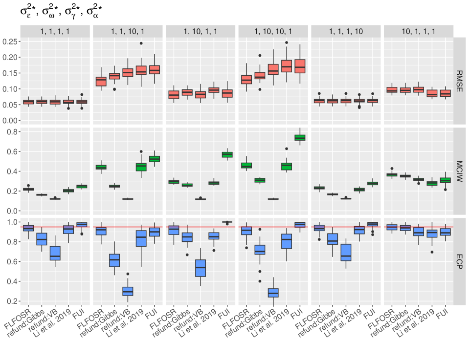
We assess the accuracy of each method by evaluating point and interval estimation for the fixed effect functions . We measure point estimation accuracy using root mean squared error for the fixed effect functions,
where and are the estimated and true fixed effects functions, respectively, for the th predictor at time . For Bayesian methods, the estimator is the posterior mean. We evaluate uncertainty quantification using mean credible/confidence interval widths,
paired with empirical coverage probability,
where are 95% credible/confidence intervals. Ideal performance is achieved by nominal coverage (calibration) and small MCIW (sharpness).
We study the impact of differing sources of variability by varying the variance components between 1 and 10 and set , , and . The results are summarized in Figure 4. Broadly, the proposed FLFOSR is highly competitive across all scenarios for both point and interval estimation. Point estimation accuracy is comparable across all methods when between-subject variability is low (), but FLFOSR offers substantial gains in point estimation accuracy as between-subject variability increases (). Notably, FLFOSR achieves close to nominal coverage across all simulation designs, while refund:Gibbs, refund:VB, and Li et al. (2022) suffer from significant undercoverage. Clearly, the VB approximation is reasonably accurate for point estimation but unreliable for uncertainty quantification. FUI is the only competitor that achieves close to nominal coverage, yet the FUI intervals are much wider than the FLFOSR intervals and thus sacrifices some power to detect important effects. Further, FUI is the least accurate point estimator when . When measurement error dominates (, the Bayesian point estimates—including for FLFOSR—are less accurate. In such high-noise settings, this performance might be improved by replacing the priors (4) with more aggressive shrinkage priors (Gao and Kowal, 2022).
In aggregate, the computational (Figures 2–3) and inferential (Figure 4) evaluations decisively favor FLFOSR. The proposed MCMC sampling algorithm (Algorithm 1) is more scalable than existing frequentist methods and more efficient than existing MCMC samplers, and delivers point and interval estimates that outperform state-of-the-art Bayesian and frequentist competitors. These significant gains amplify the additional benefits of Bayesian inference for FMMs, including uncertainty quantification for all fixed and random effects functions and predictions—which was previously not accessible even for moderately-sized datasets. By comparison, frequentist approaches typically provide inference only for the fixed effects functions, and not for the random effects functions or predictions (Li et al., 2022; Cui et al., 2022).
5 Application
We apply FLFOSR to analyze physical activity (PA) data measured from wearable accelerometry devices. These devices provide high resolution PA measurements for individual subjects across multiple days. PA plays a major role in overall human health, with lower PA levels linked to higher all-cause mortality (Schmid et al., 2015; Smirnova et al., 2020). However, statistical analysis of PA data often includes substantial aggregation or averaging both within a day and across days for a given subject (Kowal, 2022b; Hilden et al., 2023). Such pre-processing needlessly reduces the sample size and can obscure important sources of variability. In response, functional data analysis has become increasingly useful to analyze and model PA data (Sera et al., 2017; Leroux et al., 2019; Kowal and Bourgeois, 2020; Kowal, 2022a). Naturally, such approaches must confront the significant computational challenges associated with high resolution data for many individuals.
Using data from the 2005-2006 NHANES cohort, we model PA as a function of time-of-day on days for subjects . Importantly, this representation allows for analysis of time-of-day PA patterns via a FMM (1), while also accounting for within-day autocorrelations, within-subject dependencies, and measurement errors. We follow the pre-processing procedures outlined in Leroux et al. (2019) and the accompanying nhanesdata R package, which removes subjects with poor data quality or too few days of measured activity, and restrict our analysis to subjects aged 35-85. The functional data are defined by computing the square-root of 10-minute PA averages over the window , which focuses on the waking hours and helps satisfy the FMM assumptions (1). These functional data are paired with important health and demographic variables (Table 2). The continuous variables are standardized to have mean 0 and standard deviation 1. The final dataset has subjects with days of observations per subject, for a total of days of measurements, measurements per day, and predictors per subject.
| Variable | Values |
|---|---|
| Response variable: | |
| Activity Level | |
| Sociodemographic variables: | |
| Gender | Male (53%), Female (47%) |
| Age (years) | |
| Race | White (54%), Black (21%), |
| Hisp (22%), Other (4%) | |
| Education Level | HS (23%), = HS (53%), HS (24%) |
| Alcohol and drug use variables: | |
| Drinks Per Week | |
| Smoke Cigs | Current (20%), Former, (30%), Never (50%) |
| Health-related variables: | |
| Body Mass Index () | |
| HDL Cholesterol () | |
| Total Cholesterol () | |
| Systolic Blood Pressure (mmHg) | |
| Has Congestive Heart Disease | Yes , No |
| Has Congestive Heart Failure | Yes , No |
| Has Cancer | Yes , No |
| Has Diabetes | Yes , No |
| Has Stroke | Yes , No |
| Other variables: | |
| Is Weekend | Yes , No |
First, we compare the proposed FLFOSR approach with competing Bayesian methods (refund:Gibbs and refund:VB). We adopt the same hyperparameter and MCMC settings as in Section 4 and conduct a sensitive analysis in the supplementary material. However, we are unable to run refund:Gibbs or refund:VB due to memory limitations. Instead, we fit these competing methods on a random subsample of subjects, the largest subsample our memory could accommodate, solely for the purpose of computational comparisons. Table 3 shows the computational costs and MCMC efficiency for FLFOSR—fit to the whole dataset—compared to refund:Gibbs and refund:VB. FLFOSR required only about a minute to run, or about five minutes to generate 1000 effective samples from the posterior of the fixed effects functions. By comparison, refund:Gibbs required more than 21 hours to run, and due to MCMC inefficiencies, would require almost two weeks to generate 1000 effective samples—even on this much smaller dataset. Similarly, the VB approximation is dramatically slower than the FLFOSR MCMC sampling algorithm, again on the smaller dataset. Thus, the Goldsmith and Kitago (2016) strategy of (i) using VB to obtain initial estimates and (ii) using Gibbs sampling for the final results is neither necessary nor feasible: we instead should proceed exclusively with FLFOSR, which provides fully Bayesian inference on the complete dataset in a fraction of the time.
| Method | Dataset | Time () | ||
|---|---|---|---|---|
| FLFOSR | Full () | 1.3 minutes | 4.8 minutes | .27 |
| refund:Gibbs | Reduced () | 21.3 hours | 333.5 hours | .06 |
| refund:VB | Reduced () | 7.5 minutes | - | - |
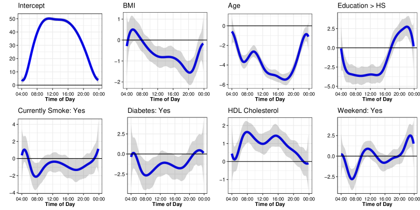
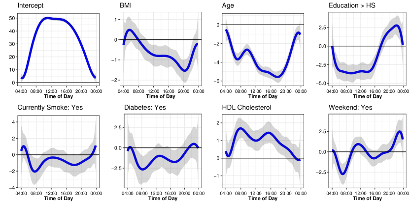
We summarize the FMM inference for select fixed effects functions in Figure 5 (see supplementary material for the remaining fixed effects functions). The results show interesting, but not necessarily unsurprising relationships between certain health factors and time-of-day PA. Age is a strong negative predictor of activity, especially in the afternoon hours. Current cigarette smokers are less active, predominantly in the morning, but this effect is not as strong later in the day. Individuals with higher educational attainment are less active throughout the daytime, but more active after in the early evening. Among health variables, certain comorbidities like diabetes are associated with less activity. HDL cholesterol, commonly referred to as “good cholesterol”, is associated with higher activity throughout the day.

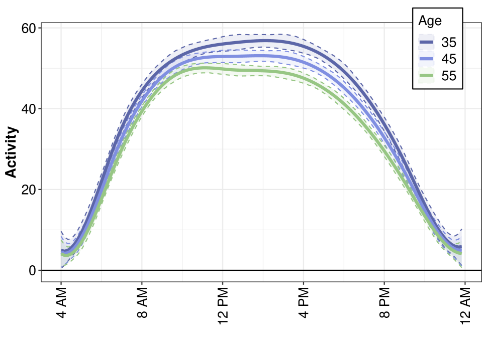
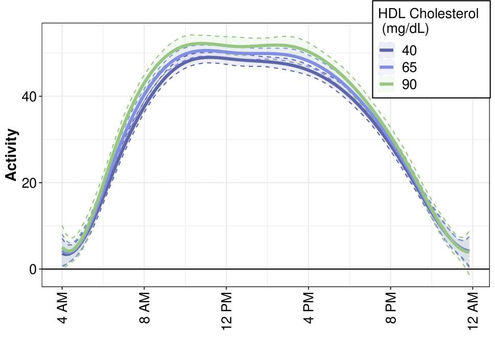
As an alternative visualization of these effects, Figure 6 shows the predicted population-level mean activity for varying levels of (a) age and (b) HDL cholesterol. The other predictors were set to the baseline and the mean values for categorical and continuous variables, respectively. As age increases from 35 to 55, there is a substantial overall decrease in predicted PA, which is particularly pronounced in the afternoon. HDL cholesterol levels in the data ranged from 23 mg/dL to 188 mg/dL, but levels below 40 mg/dL are broadly classified as “at risk” of heart disease and are generally recommended to be above 60 mg/dL (Expert Panel, 2001). The right hand plot shows the predicted activity curves when raising HDL levels from the lower cutoff point up into the recommended amount, where slightly heightened PA throughout waking hours is predicted as HDL levels increase.
6 Discussion
We introduced a new MCMC algorithm for Bayesian regression with longitudinal functional data. The algorithm applies for a broad and widely-useful class of functional mixed models that include (i) basis expansions and (ii) fixed effects and subject- and replicate-specific random effects. Most notably, our MCMC sampler delivers unrivaled MCMC efficiency and unmatched computational scalability, and is empirically faster than state-of-the-art frequentist competitors—while also providing posterior uncertainty quantification for all model parameters and predictions. The scalability of our algorithm persists across all dimensions—the number subjects, replicates per subjects, and covariates—and thus establishes a new state-of-the-art for (Bayesian or frequentist) computing with longitudinal functional data. The proposed model showcases excellent point estimation accuracy and uncertainty quantification across a broad array of simulated data scenarios.
In practice, our MCMC algorithm enables complex Bayesian model-fitting with large functional datasets without the need for intensive computing resources. Indeed, we were able to perform fully Bayesian inference on a large physical activity (PA) dataset in about a minute using a personal desktop without any parallel processing. As the usage of wearable devices continues to grow, so does the need for highly scalable methods to study these high-resolution and high-dimensional data. For example, the UK Biobank study contains PA measurements of over 100,000 subjects across 7 days, measured in 5 second intervals (Doherty et al., 2017), implying over 12 billion rows of PA measurements.
To meet these computational burdens, future work will consider EM algorithms and VB approximations based on the same core ideas as the proposed MCMC algorithm (Algorithm 1). We expect that such strategies would further increase computational scalability, but at the cost of reliable (posterior) uncertainty quantification.
One computational aspect that we did not explore in this paper is the memory usage of each algorithm. For the NHANES data, memory issues precluded use of the competing methods in the refund package on the whole dataset, while the proposed FLFOSR approach encountered no such problems. Thus, efficient memory usage may be another advantage of FLFOSR, but further analysis is needed.
SUPPLEMENTARY MATERIAL
- Additional results:
-
A document containing a sensitivity analysis and additional results for the application. (PDF)
- R code:
-
Code for model implementation and producing all results and plots in the paper. (Zipped file)
References
- Besse et al. (2000) Besse, P. C., H. Cardot, and D. B. Stephenson (2000). Autoregressive Forecasting of Some Functional Climatic Variations. Scandinavian Journal of Statistics 27(4), 673–687.
- Bhattacharya et al. (2016) Bhattacharya, A., A. Chakraborty, and B. K. Mallick (2016). Fast sampling with Gaussian scale mixture priors in high-dimensional regression. Biometrika 103(4), 985–991.
- Boschi et al. (2021) Boschi, T., J. Di Iorio, L. Testa, M. A. Cremona, and F. Chiaromonte (2021). Functional data analysis characterizes the shapes of the first COVID-19 epidemic wave in Italy. Scientific Reports 11(1), 17054.
- Cederbaum et al. (2016) Cederbaum, J., M. Pouplier, P. Hoole, and S. Greven (2016). Functional linear mixed models for irregularly or sparsely sampled data. Statistical Modelling 16(1), 67–88.
- Cui et al. (2022) Cui, E., A. Leroux, E. Smirnova, and C. M. Crainiceanu (2022). Fast Univariate Inference for Longitudinal Functional Models. Journal of Computational and Graphical Statistics 31(1), 219–230.
- Doherty et al. (2017) Doherty, A., D. Jackson, N. Hammerla, T. Plötz, P. Olivier, M. H. Granat, T. White, V. T. van Hees, M. I. Trenell, C. G. Owen, S. J. Preece, R. Gillions, S. Sheard, T. Peakman, S. Brage, and N. J. Wareham (2017). Large Scale Population Assessment of Physical Activity Using Wrist Worn Accelerometers: The UK Biobank Study. PLOS ONE 12(2), e0169649.
- Expert Panel (2001) Expert Panel (2001). Executive Summary of the Third Report of the National Cholesterol Education Program (NCEP) Expert Panel on Detection, Evaluation, and Treatment of High Blood Cholesterol in Adults (Adult Treatment Panel III). Journal of the American Medical Association 285(19), 2486–2497.
- Gao and Kowal (2022) Gao, Y. and D. R. Kowal (2022). Bayesian adaptive and interpretable functional regression for exposure profiles. arXiv preprint arXiv:2203.00784.
- Gelman (2006) Gelman, A. (2006). Prior distributions for variance parameters in hierarchical models. Bayesian Analysis 1(3).
- Gelman et al. (2013) Gelman, A., J. B. Carlin, H. S. Stern, D. B. Dunson, A. Vehtari, and D. B. Rubin (2013). Bayesian Data Analysis (3rd ed ed.). CRC Press.
- Goldsmith and Kitago (2016) Goldsmith, J. and T. Kitago (2016). Assessing systematic effects of stroke on motor control by using hierarchical function-on-scalar regression. Journal of the Royal Statistical Society: Series C (Applied Statistics) 65(2), 215–236.
- Goldsmith et al. (2021) Goldsmith, J., F. Scheipl, L. Huang, J. Wrobel, C. Di, J. Gellar, J. Harezlak, M. W. McLean, B. Swihart, L. Xiao, C. Crainiceanu, and P. T. Reiss (2021). refund: Regression with Functional Data. R package version 0.1-24.
- Goldsmith et al. (2015) Goldsmith, J., V. Zipunnikov, and J. Schrack (2015). Generalized multilevel function-on-scalar regression and principal component analysis. Biometrics 71(2), 344–353.
- Guo (2002) Guo, W. (2002). Functional Mixed Effects Models. Biometrics 58(1), 121–128.
- Hilden et al. (2023) Hilden, P., J. E. Schwartz, C. Pascual, K. M. Diaz, and J. Goldsmith (2023). How many days are needed? Measurement reliability of wearable device data to assess physical activity. PLOS ONE 18(2), e0282162.
- Huo et al. (2022) Huo, S., J. S. Morris, and H. Zhu (2022). Ultra-Fast Approximate Inference Using Variational Functional Mixed Models. Journal of Computational and Graphical Statistics, 1–32.
- Kowal (2022a) Kowal, D. R. (2022a). Fast, Optimal, and Targeted Predictions Using Parameterized Decision Analysis. Journal of the American Statistical Association 117(540), 1875–1886.
- Kowal (2022b) Kowal, D. R. (2022b). Subset selection for linear mixed models. Biometrics, biom.13707.
- Kowal and Bourgeois (2020) Kowal, D. R. and D. C. Bourgeois (2020). Bayesian Function-on-Scalars Regression for High-Dimensional Data. Journal of Computational and Graphical Statistics 29(3), 629–638.
- Kowal et al. (2019) Kowal, D. R., D. S. Matteson, and D. Ruppert (2019). Functional Autoregression for Sparsely Sampled Data. Journal of Business & Economic Statistics 37(1), 97–109.
- Lee et al. (2019) Lee, W., M. F. Miranda, P. Rausch, V. Baladandayuthapani, M. Fazio, J. C. Downs, and J. S. Morris (2019). Bayesian Semiparametric Functional Mixed Models for Serially Correlated Functional Data, With Application to Glaucoma Data. Journal of the American Statistical Association 114(526), 495–513.
- Leroux et al. (2019) Leroux, A., J. Di, E. Smirnova, E. J. Mcguffey, Q. Cao, E. Bayatmokhtari, L. Tabacu, V. Zipunnikov, J. K. Urbanek, and C. Crainiceanu (2019). Organizing and Analyzing the Activity Data in NHANES. Statistics in Biosciences 11(2), 262–287.
- Li et al. (2022) Li, R., L. Xiao, E. Smirnova, E. Cui, A. Leroux, and C. M. Crainiceanu (2022). Fixed‐effects inference and tests of correlation for longitudinal functional data. Statistics in Medicine 41(17), 3349–3364.
- Liebl (2013) Liebl, D. (2013). Modeling and forecasting electricity spot prices: A functional data perspective. The Annals of Applied Statistics 7(3).
- Morris (2017) Morris, J. S. (2017). Comparison and contrast of two general functional regression modelling frameworks. Statistical Modelling 17(1-2), 59–85.
- Morris and Carroll (2006) Morris, J. S. and R. J. Carroll (2006). Wavelet-based functional mixed models. Journal of the Royal Statistical Society: Series B (Statistical Methodology) 68(2), 179–199.
- Nishimura and Suchard (2022) Nishimura, A. and M. A. Suchard (2022). Prior-Preconditioned Conjugate Gradient Method for Accelerated Gibbs Sampling in “Large n , Large p ” Bayesian Sparse Regression. Journal of the American Statistical Association, 1–14.
- Park and Staicu (2015) Park, S. Y. and A.-M. Staicu (2015). Longitudinal functional data analysis. Stat 4(1), 212–226.
- Reiss et al. (2010) Reiss, P. T., L. Huang, and M. Mennes (2010). Fast Function-on-Scalar Regression with Penalized Basis Expansions. The International Journal of Biostatistics 6(1).
- Rue (2001) Rue, H. (2001). Fast Sampling of Gaussian Markov Random Fields. Journal of the Royal Statistical Society Series B: Statistical Methodology 63(2), 325–338.
- Scheipl et al. (2012) Scheipl, F., L. Fahrmeir, and T. Kneib (2012). Spike-and-Slab Priors for Function Selection in Structured Additive Regression Models. Journal of the American Statistical Association 107(500), 1518–1532.
- Scheipl et al. (2016) Scheipl, F., J. Gertheiss, and S. Greven (2016). Generalized functional additive mixed models. Electronic Journal of Statistics 10(1).
- Scheipl et al. (2015) Scheipl, F., A.-M. Staicu, and S. Greven (2015). Functional Additive Mixed Models. Journal of Computational and Graphical Statistics 24(2), 477–501.
- Schmid et al. (2015) Schmid, D., C. Ricci, and M. F. Leitzmann (2015). Associations of Objectively Assessed Physical Activity and Sedentary Time with All-Cause Mortality in US Adults: The NHANES Study. PLOS ONE 10(3), e0119591.
- Sera et al. (2017) Sera, F., L. J. Griffiths, C. Dezateux, M. Geraci, and M. Cortina-Borja (2017). Using functional data analysis to understand daily activity levels and patterns in primary school-aged children: Cross-sectional analysis of a UK-wide study. PLOS ONE 12(11), e0187677.
- Sergazinov et al. (2023) Sergazinov, R., A. Leroux, E. Cui, C. Crainiceanu, R. N. Aurora, N. M. Punjabi, and I. Gaynanova (2023). A case study of glucose levels during sleep using multilevel fast function on scalar regression inference. Biometrics, biom.13878.
- Smirnova et al. (2020) Smirnova, E., A. Leroux, Q. Cao, L. Tabacu, V. Zipunnikov, C. Crainiceanu, and J. K. Urbanek (2020). The Predictive Performance of Objective Measures of Physical Activity Derived From Accelerometry Data for 5-Year All-Cause Mortality in Older Adults: National Health and Nutritional Examination Survey 2003–2006. The Journals of Gerontology: Series A 75(9), 1779–1785.
- Yu and Meng (2011) Yu, Y. and X.-L. Meng (2011). To Center or Not to Center: That Is Not the Question—An Ancillarity–Sufficiency Interweaving Strategy (ASIS) for Boosting MCMC Efficiency. Journal of Computational and Graphical Statistics 20(3), 531–570.
- Zhu et al. (2011) Zhu, H., P. J. Brown, and J. S. Morris (2011). Robust, Adaptive Functional Regression in Functional Mixed Model Framework. Journal of the American Statistical Association 106(495), 1167–1179.
- Zhu et al. (2019) Zhu, H., K. Chen, X. Luo, Y. Yuan, and J.-L. Wang (2019). FMEM: Functional Mixed Effects Models for Longitudinal Functional Responses. Statistica Sinica 29(4), 2007–2033.
- Zipunnikov et al. (2014) Zipunnikov, V., S. Greven, H. Shou, B. S. Caffo, D. S. Reich, and C. M. Crainiceanu (2014). Longitudinal high-dimensional principal components analysis with application to diffusion tensor imaging of multiple sclerosis. The Annals of Applied Statistics 8(4).
Supplement
A Additional Simulation Results
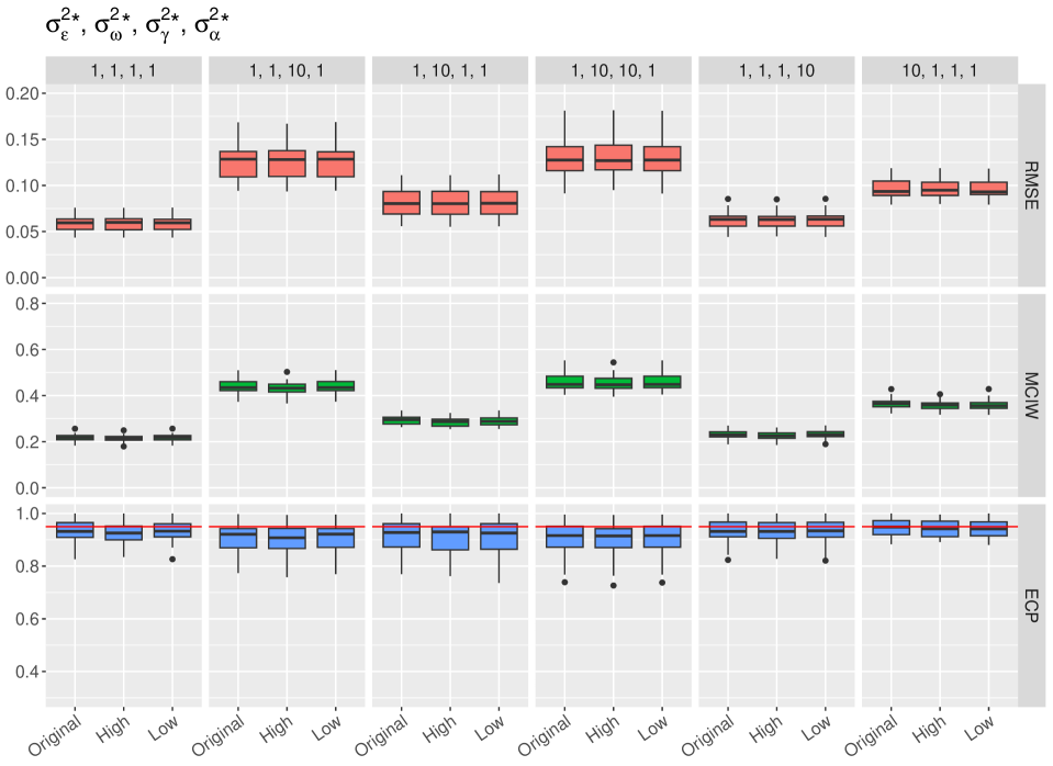
We perform a sensitivity analysis to investigate how choice of hyperparameter values for the inverse-gamma priors on and affects the simulation results. We set hyperparameter values as , , , as high values, and , , , as low values. Figure S1 shows the original results of our model from the simulation study in Section 4.4 along with the same simulations but with high and low hyperparameter values. The results show generally low sensitivity to choice of variance hyperparameters.
B Additional Application Results
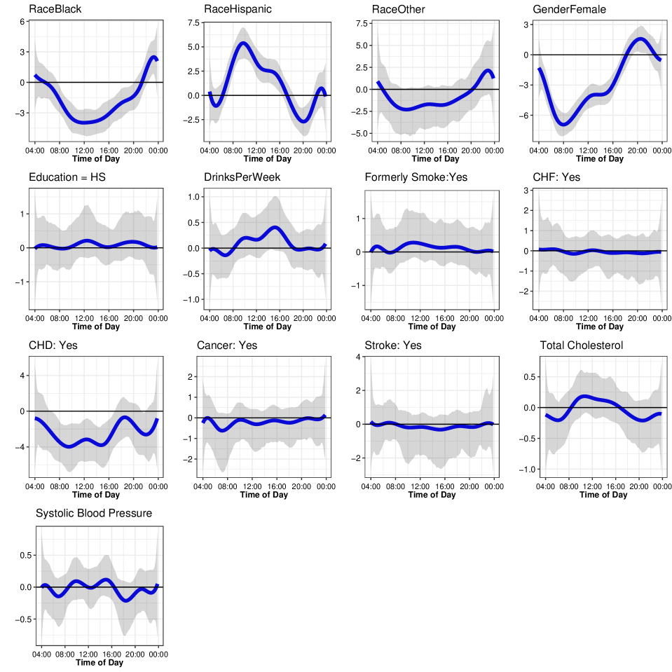
For the results from our data application in Section 5, Figure S3 shows the rest of the fixed effect functions for model covariates not shown in Figure 5. Certain health conditions such as cancer, stroke, and congestive heart failure seem to have close to zero effect on activity throughout the day, along with a large uncertainty band. Although, congestive heart disease may have a meaningful negative association in the morning and afternoon. Only a small percentage of the sample reported having any of these conditions (Table 2). Race and gender seem to be strong predictors of physical activity, whereas other effects were not a strong, such as drinks per week or being a former smoker (compared to non-smoker).
Figure S2 shows a sensitivity analysis of the estimated fixed effect regression functions and 95% credible intervals akin to Figure 5. Again, we set hyperparameter values as , , , as high values, and , , , as low values. The results are almost identical to each other and the original estimates, showing robustness to choice of hyperparameters. This is likely in part due to the large sample size of the NHANES dataset.