Goal-Oriented Adaptive Space-Time Finite Element Methods
for Regularized Parabolic p-Laplace Problems

Abstract

We consider goal-oriented adaptive space-time finite-element discretizations of the regularized parabolic p-Laplace problem on completely unstructured simplicial space-time meshes. The adaptivity is driven by the dual-weighted residual (DWR) method since we are interested in an accurate computation of some possibly nonlinear functionals at the solution. Such functionals represent goals in which engineers are often more interested than the solution itself. The DWR method requires the numerical solution of a linear adjoint problem that provides the sensitivities for the mesh refinement. This can be done by means of the same full space-time finite element discretization as used for the primal non-linear problems. The numerical experiments presented demonstrate that this goal-oriented, full space-time finite element solver efficiently provides accurate numerical results for different functionals.

Keywords: Regularized parabolic p-Laplacian, space-time finite element discretization, goal-oriented adaptivity

2020 MSC: 35K61, 65M50, 65M60

1 Introduction

In this paper, we investigate goal-oriented adaptive space-time (GOAST) finite element discretizations of initial-boundary value problems (IBVP) for the scalar regularized parabolic $p$-Laplace equation

$$\partial_{t}u-\mathrm{div}_{x}((|\nabla_{x}u|^{2}+\varepsilon^{2})^{\frac{p-2}{2}}\nabla_{x}u)=f\;\text{in}\;Q,\quad u=u_{D}:=0\;\text{on}\;\Sigma,\quad u=u_{0}:=0\;\text{on}\;\overline{\Sigma}_{0}$$ (1)

on completely unstructured simplicial space-time meshes, where $Q=\Omega\times(0,T)\subset\mathbb{R}^{d+1}$ denotes the space-time cylinder, $\Sigma=\partial{\Omega}\times(0,T)$ its lateral surface where the Dirichlet boundary condition $u_{D}$ is prescribed, $\Sigma_{0}=\Omega\times\{0\}$ its bottom where the initial condition $u_{0}$ is given, $\Omega\subset\mathbb{R}^{d}$ with the boundary $\partial{\Omega}$ denotes the spatial domain that is supposed to be bounded and Lipschitz, $d\in\{1,2,3\}$ is the spatial dimension, $T>0$ is the final time, the right-hand side $f$ is a given source driving the evolution process, the given power $p\in(1,\infty)$ characterizes the nonlinearity of the evolution, and $\varepsilon>0$ is a positive regularization parameter.

In the limit case $\varepsilon=0$, we speak about the original parabolic $p$-Laplace problem that corresponds to the simple (linear) transient heat problem for $p=2$, but that can degenerate otherwise. As usual, $\nabla_{x}$, $\text{div}_{x}$, and $\partial_{t}$ stand for the spatial gradient, the spatial divergence, and the partial time-derivative, respectively, whereas $|\nabla_{x}u|=\big{(}\sum_{i=1}^{d}|\partial_{i}u|^{2}\big{)}^{1/2}$ denotes the Euclidean norm of the spatial gradient $\nabla_{x}u=(\partial_{1}u,\ldots,\partial_{d}u)^{\top}{}$ of $u$. We note that the regularized parabolic $p$-Laplace equation is sometimes written in the form $\partial_{t}u-\mathrm{div}_{x}((|\nabla_{x}u|+\varepsilon)^{p-2}\nabla_{x}u)=f$ instead of (1); see, e.g., the book [55], in particular, Exercises 4.26 therein, or the recent works [62, 40, 39]. There are many publications on the solvability analysis including investigations of the regularity of the solution [65, 21, 55, 17], the numerical solution including discretization error estimates [7] and solvers for the nonlinear finite element equations [48], and applications of elliptic (stationary) and parabolic (evolutionary) $p$-Laplace models in different disciplines [20], and the references therein.

The standard numerical technique for the discretization of parabolic $p$-Laplace problems like (1) uses some time-stepping for the temporal discretization in combination with a spatial finite element Galerkin discretization; see, e.g., [7]. In contrast to this traditional approach, we here propose to use a completely unstructured space-time finite element method on simplicial space-time meshes that finally leads to the solution of one nonlinear system of finite element equations instead of many smaller nonlinear systems in the case of implicit time-stepping. This space-time approach has successfully been used for linear parabolic initial boundary value problems; see, e.g. the survey article [60]. Concerning the parabolic $p$-Laplace initial-boundary value problem, we are only aware of the very recent publication [62] by Toulopoulos who derived consistent space-time finite element schemes that are stabilized by adding additional time-upwind and interface-jump terms. These stabilizations allow him to prove a priori discretization error estimates in some mesh-dependent norm as was done in the papers [43] or [44] for linear parabolic initial-boundary value problems.

In this paper, we consider goal-oriented adaptive space-time finite element Galerkin discretizations of the regularized variational $p$-Laplace problem for $p\in(1,\infty)$ without any further stabilization. In goal oriented error estimations [10, 22, 32, 50, 33, 35], we aim at the estimation of the error in some quantities of interest, also called goal functionals. For information about the treatment of multiple goal functionals at once see [38, 37, 1, 41, 2, 11, 25]. In this work, we use the dual weighted residual (DWR) method [9, 10], where the localization of the error estimator is done by the partition-of-unity (PU) technique [53]. For other localization techniques, we refer to [10, 8, 14].

The DWR method additionally requires the solution of the adjoint problem that is linear, but backward in time. So we can basically use the same space-time finite element discretization as for the primal problem. This is one advantage of fully unstructured space-time finite element methods that was already used for parabolic optimal control problems where the adjoint problem appears in the first-order optimality system; see, e.g., [47, 46, 57, 45]. The goal-oriented adaptivity can now be done simultaneously in space and time like in the elliptic case since the time $t$ is just another variable. The same is true for a simultaneous parallelization of the final numerical algorithm. These are two other benefits of the unstructured space-time approach over the more traditional time-stepping.

The remainder of the paper is organized as follows. In Section 2, we derive the space-time variational formulation of the regularized $p$-Laplace initial-boundary value problem (1), and introduce some notations and preliminary results. This variational formulation is the starting point for the space-time finite element discretization that is presented in Section 3 together with the Newton linearization of the discrete problem. Section 4 is devoted to the description of the goal-oriented space-time adaptive procedure that is driven by the DWR method and their localization by the PU technique. In Section 5, we present and discuss some numerical results for two different goal functionals.

Finally, we draw some conclusions, and give an outlook on some further research topics.

2 Space-Time Variational Formulations

Multiplying the parabolic $p$-Laplace equation by a test function $v\in V:=L_{p}((0,T);\mathring{W}_{p}^{1}(\Omega))$, integrating over $Q$, and integrating by parts in the nonlinear elliptic term, we arrive at the following variational formulation: Find $u\in U:=\{v\in V:\partial_{t}v\in V^{*},v=0\;\mbox{on}\;\Sigma_{0}\}$ such that

$$\langle\partial_{t}u,v\rangle+((|\nabla_{x}u|^{2}+\varepsilon^{2})^{\frac{p-2}{2}}\nabla_{x}u,\nabla_{x}v)=\langle f,v\rangle\quad\forall\,v\in V,$$ (2)

where $\langle\cdot,\cdot\rangle:V^{*}\times V\rightarrow\mathbb{R}$ and $(\cdot,\cdot):H\times H\rightarrow\mathbb{R}$ denote the duality and the $H=L_{2}(Q)$-inner product, respectively. The given source function $f$ should belong to $V^{*}:=L_{q}((0,T);W_{q}^{-1}(\Omega))$ that is the dual space of $V$, where $q=p/(p-1)$ denotes Hölder’s conjugate of $p$. Here and throughout the paper, we use the usual notations for Sobolev and Bochner spaces; see, e.g., [65], where the norms in the trial space $U$ and the test space $V$ are defined by

$$\|u\|_{U}=\|u\|_{V}+\|\partial_{t}u\|_{V^{*}}\quad\mbox{and}\quad\|u\|_{V}=\|\nabla_{x}u\|_{L_{p}(Q)}:=\||\nabla_{x}u|\|_{L_{p}(Q)}=\Big{(}\int_{Q}\big{(}\sum_{i=1}^{d}|\partial_{i}v|^{2}\big{)}^{p/2}\Big{)}^{1/p},$$

respectively, with $\|f\|_{V^{*}}=\sup_{v\in V}\langle f,v\rangle/\|v\|_{V}$. We mention that, instead of the standard $L_{p}$ norm for vector functions, we use the equivalent norm $\||\cdot|\|_{L_{p}(Q)}$ that is better suited for investigating the $p$-Laplace problem. The variational problem (2) has a unique solution $u$ that belongs to $U\cap C([0,T];L_{2}(\Omega))$. This solvability result for (2) including the case $\varepsilon=0$ follows from standard monotonicity arguments; see, e.g., [49], [65] and [55]. In particular, it has recently been proved in [17] that, under additional regularity assumptions imposed on $\Omega$ and under the assumptions that

$$f\in L_{2}(Q)\quad\mbox{and}\quad u_{0}\in\mathring{W}_{p}^{1}(\Omega),$$

there is a unique approximable solution to (1) for $\varepsilon=0$ such that $u\in L_{\infty}((0,T);\mathring{W}_{p}^{1}(\Omega))$, $\partial_{t}u\in L_{2}(Q)$ and $|\nabla_{x}u|^{p-2}\nabla_{x}u\in L_{2}((0,T);W_{2}^{1}(\Omega))$, i.e. the $p$-Laplace equation (1) holds in the strong sense in $L_{2}(Q)$. Moreover, the corresponding a priori estimates are proven in same paper; see Theorem 2.1 and Theorem 2.2 in [17]. Further regularity results can be found, e.g., in [65] and [55].

The nonlinear variational problem (2) can be rewritten as nonlinear operator equation: Find $u\in U$ such that

$$\mathcal{A}(u):=\partial_{t}u+A(u)-f=0\quad\mbox{in}\,V^{*},$$ (3)

where the nonlinear operator $\mathcal{A}:U\mapsto V^{*}$ is defined by the variational identity

$$\mathcal{A}(u)(v)=\langle\mathcal{A}(u),v\rangle:=\langle\partial_{t}u,v\rangle+\langle A(u),v\rangle-\langle f,v\rangle\quad\forall\,v\in V,\;\forall\,u\in U,$$

with $\langle A(u),v\rangle:=((|\nabla_{x}u|^{2}+\varepsilon^{2})^{\frac{p-2}{2}}\nabla_{x}u,\nabla_{x}v)$.

3 Space-Time Finite Element Discretization and Linearization

We are now going to construct finite element schemes as Galerkin approximations to (2) on fully unstructured simplicial decompositions of the space-time cylinder $Q$. Let $\mathcal{T}_{h}=\{\Delta\}$ be a decomposition (mesh) of $Q$ into non-overlapping shape-regular simplicial finite elements $\Delta$ (triangles, tetrahedra and pentatops for $d=1,2$, and $3$, respectively) such that $\overline{Q}=\bigcup_{\Delta\in\mathcal{T}_{h}}\overline{\Delta}$. So, for simplicity, we here and in the following assume that the spacial domain $\Omega$ is polytopic. The discretization parameter $h$ should indicate that, in fact, we consider a family of finer and finer meshes, where the refinement can be done adaptively; see, e.g., [15, 31, 58] for a precise description of such families of shape-regular meshes and their construction.
After choosing the space-time finite element mesh $\mathcal{T}_{h}$, we can define space-time finite element subspaces

$$U_{h}=V_{h}:=\{v_{h}\in S_{h}^{k}(\overline{Q}):\,v_{h}=0\;\mbox{on}\;{\overline{\Sigma}}{\cup{\overline{\Sigma}}_{0}}\}\subset U\subset V,$$

where $S_{h}^{k}(\overline{Q})=\{v_{h}\in C(\overline{Q}):v_{h}({\tt x}_{\Delta}(\cdot))\in\mathbb{P}_{k}(\widehat{\Delta}),\,\forall\Delta\in\mathcal{T}_{h}\}$ is nothing but the standard finite element space based on polynomials of the degree $k\in\mathbb{N}:=\{1,2,\dots\}$. The regular map ${\tt x}_{\Delta}(\cdot)=(x_{1}(\cdot),\ldots,x_{d+1}(\cdot)):\widehat{\Delta}\rightarrow\Delta$ maps the reference element $\widehat{\Delta}$ (unit simplex) to the finite element $\Delta\in\mathcal{T}_{h}$, and $\mathbb{P}_{k}(\widehat{\Delta})$ denotes the space of polynomials of degree $k$ on the reference element $\widehat{\Delta}$. We look at the time $t$ as just another coordinate direction $x_{d+1}$. Here and in our numerical experiments in Section 5, we only consider affine-linear mappings ${\tt x}_{\Delta}(\cdot)$ since we assumed polytopic spacial domains for simplicity. In this case, the finite element space $S_{h}^{k}(\overline{Q})$ consists of all continuous and piecewise polynomial functions. It is clear that we can use more general curved elements realized by the mapping that would not only admit curved spatial domains but also changing spatial domains in time leading to curved, but geometrically fixed space-time “cylinders” $Q$. If the Jacobians of the mapping ${\tt x}_{\Delta}(\cdot)$ fulfil the standard regularity properties, then the usual approximations properties hold; see. e.g, [15, 31, 58].

Once the finite element trial and test spaces $U_{h}$ and $V_{h}=U_{h}$ are defined, we can look for a space-time finite element solution $u_{h}\in U_{h}$ such that

$$\mathcal{A}(u_{h})(v_{h})\equiv\langle\mathcal{A}(u_{h}),v_{h}\rangle:=\langle\partial_{t}u_{h},v_{h}\rangle+\langle A(u_{h}),v_{h}\rangle-\langle f,v_{h}\rangle=0\quad\forall\,v_{h}\in V_{h}=U_{h}.$$ (4)

The space-time finite element Galerkin scheme has a unique solution. The existence follows, e.g., from the proof of Lemma 8.95 in [55] where such kind of space-time Galerkin schemes were used to proof the existence to weak solutions of non-linear parabolic initial-boundary value problems like (1). The uniqueness of the finite element solution is a consequence of fact that the Jacobian is uniformly positive definite for fixed $\varepsilon$, $p$, $d$, and $h$; see the estimates given below.

Let the finite element spaces $U_{h}=V_{h}=\mbox{span}\{\varphi_{j}:j=1,\ldots,N_{h}\}$ be spanned by the standard nodal finite element basis. Then the finite element solution $u_{h}=\sum_{j=1}^{N_{h}}u_{j}\varphi_{j}$ of (4) can be defined by the solution $\mathbf{u}_{h}=(u_{1},\ldots,u_{N_{h}})^{\top}{}\in\mathbb{R}^{N_{h}}$ of the non-linear system of finite element equations

$$\mathcal{A}_{h}(\mathbf{u}_{h})=0\quad\mbox{in}\;\mathbb{R}^{N_{h}},$$ (5)

where the image $\mathcal{A}_{h}(\mathbf{u}_{h})$ of the non-linear map $\mathcal{A}_{h}:\mathbb{R}^{N_{h}}\rightarrow\mathbb{R}^{N_{h}}$ at some given vector $\mathbf{u}_{h}\in\mathbb{R}^{N_{h}}$ can be computed by the formula

$$\mathcal{A}_{h}(\mathbf{u}_{h})=T_{h}\mathbf{u}_{h}+\widehat{A}_{h}(\mathbf{u}_{h})\mathbf{u}_{h}-\mathbf{f}_{h}.$$ (6)

The $N_{h}\times N_{h}$ matrices $T_{h}$ and $\widehat{A}_{h}(\mathbf{u}_{h})$ are defined by the variational identities

$$(T_{h}\mathbf{w}_{h},\mathbf{v}_{h})_{\ell_{2}}=\langle\partial_{t}w_{h},v_{h}\rangle\;\mbox{and}\;(\widehat{A}_{h}(\mathbf{u}_{h})\mathbf{w}_{h},\mathbf{v}_{h})_{\ell_{2}}=((|\nabla_{x}u_{h}|^{2}+\varepsilon^{2})^{\frac{p-2}{2}}\nabla_{x}w_{h},\nabla_{x}v_{h})\;$$ (7)

for all $w_{h},v_{h}\in U_{h}=V_{h}$, respectively, whereas the vector $\mathbf{f}_{h}=(\langle f,\varphi_{i}\rangle)_{i=1,\ldots,N_{h}}\in\mathbb{R}^{N_{h}}$ can easily be computed from the given source term $f\in V^{*}$. The matrix $T_{h}$ is non-symmetric, but non-negative, whereas the matrix $\widehat{A}_{h}(\mathbf{u}_{h})$ is always symmetric and positive definite (spd) provided that $\varepsilon^{2}>0$, otherwise it is always non-negative. The unique solvability of the nonlinear system (6) follows from the unique solvability of the finite element scheme (4).

The non-linear system (5) can be solved by means of the Newton method that reads as follows: For given initial guess $\mathbf{u}_{h}^{0}\in\mathbb{R}^{N_{h}}$, find $\mathbf{u}_{h}^{n+1}=\mathbf{u}_{h}^{n}+\mathbf{w}_{h}^{n+1}$ via the Newton correction $\mathbf{w}_{h}^{n+1}\in\mathbb{R}^{N_{h}}$ that is nothing but the unique solution of the linear system

$$\mathcal{A}^{\prime}_{h}(\mathbf{u}_{h}^{n})\mathbf{w}_{h}^{n+1}=-\mathcal{A}_{h}(\mathbf{u}_{h}^{n}),\quad n=0,1,\ldots,$$

with the Jacobian $\mathcal{A}^{\prime}_{h}(\mathbf{u}_{h}^{n})=T_{h}+\widehat{A}_{h}(\mathbf{u}_{h}^{n})+\widehat{A}^{\prime}_{h}(\mathbf{u}_{h}^{n})$, where the matrices $T_{h}$ and $\widehat{A}_{h}(\mathbf{u}_{h}^{n})$ are given by (7), and the matrix $\widehat{A}^{\prime}_{h}(\mathbf{u}_{h}^{n})$ is defined by the identity

$$(\widehat{A}^{\prime}_{h}(\mathbf{u}_{h}^{n})\mathbf{w}_{h},\mathbf{v}_{h})_{\ell_{2}}=(p-2)(((|\nabla_{x}{u}_{h}^{n}|^{2}+\varepsilon^{2})^{\frac{p-4}{2}}\nabla_{x}{u}_{h}^{n}(\nabla_{x}{u}_{h}^{n})^{\top}{})\nabla_{x}w_{h},\nabla_{x}v_{h})$$

for all $w_{h},v_{h}\in U_{h}$ associated to the vectors $\mathbf{w}_{h},\mathbf{v}_{h}\in\mathbb{R}^{N_{h}}$. The Jacobian is positive definite for $\varepsilon>0$. Indeed, for $p>1$, we have

$$(\mathcal{A}^{\prime}_{h}(\mathbf{u}_{h}^{n})\mathbf{w}_{h},\mathbf{w}_{h})_{\ell_{2}}= \;(\partial_{t}w_{h},w_{h})+((|\nabla_{x}u_{h}^{n}|^{2}+\varepsilon^{2})^{\frac{p-2}{2}}\nabla_{x}w_{h},\nabla_{x}w_{h})$$

$$+(p-2)(((|\nabla_{x}{u}_{h}^{n}|^{2}+\varepsilon^{2})^{\frac{p-4}{2}}\nabla_{x}{u}_{h}^{n}(\nabla_{x}{u}_{h}^{n})^{\top}{})\nabla_{x}w_{h},\nabla_{x}w_{h})$$

$$\geq\frac{1}{2}\|w_{h}(\cdot,T)\|_{L_{2}(\Omega)}^{2}+c(p,\varepsilon)\|\nabla_{x}w_{h}\|_{L_{2}(Q)}^{2}\geq c(p,\varepsilon)ch^{d+1}(\mathbf{w}_{h},\mathbf{w}_{h})_{\ell_{2}}$$

for all $w_{h}\in U_{h}$ corresponding to the coefficient vector $\mathbf{w}_{h}\in\mathbb{R}^{N_{h}}$ via the finite element isomorphism, where $c(p,\varepsilon)=(p-1)\varepsilon^{p-2}$ and $c(p,\varepsilon)=\varepsilon^{p-2}$ for $p\in(1,2)$ and $p\in[2,\infty)$, respectively. Thus, the Newton method is always well-defined.

4 Goal-Oriented Adaptive Space-Time Finite Element Methods

In many applications, the solution $u$ itself is often not of primary interest, but some quantity of interest represented by some (possibly nonlinear) functional $J:U\mapsto\mathbb{R}$ evaluated at the solution $u$. Such quantities could be the average of the solution or the gradient of the solution in some subregion of the space-time cylinder, or a regularized point evaluation; see also the quantity of interest used in our numerical experiments in Section 5. The aim is to approximate $J(u)$ as well as possible using as few as possible degrees of freedom. Of course, instead of $J(u)$, we can only compute the functional at the finite element solution $u_{h}$, i.e. $J(u_{h})$. Therefore, we are interested in evaluation of the error $J(u)-J(u_{h})$. To estimate the error, we use the dual weighted residual method as described in [9, 10, 52]. Other GOAST methods using time-slabs or a recuded order basis can be found in [42, 54, 34].

4.1 The primal and the adjoint problems

The primal problem is nothing but the variational problem (3), and it defines the solution $u\in U$. Its discretization is given by the finite element scheme (4) defining the finite element solution $u_{h}\in U_{h}$ approximating $u$.

To connect the functional $J$ with the initial-boundary value problem (3), we consider the adjoint problem. The formal adjoint problem reads as follows: Find $z\in V$ such that

$$\mathcal{A}^{\prime}(u)(v,z):=\langle\partial_{t}v,z\rangle+A^{\prime}(u)(v,z)=J^{\prime}(u)(v)\quad\forall v\in U,$$ (8)

where $u$ solves the primal problem (3), and

$$A^{\prime}(u)(v,z)=(((|\nabla_{x}u|^{2}+\varepsilon^{2})^{\frac{p-2}{2}}I+(p-2)(|\nabla_{x}u|^{2}+\varepsilon^{2})^{\frac{p-4}{2}}\nabla_{x}u(\nabla_{x}u)^{\top}{})\nabla_{x}v,\nabla_{x}z).$$

To obtain $z$ we still have to solve a linear PDE problem that is nothing but a well-posed backward parabolic problem. Therefore, the adjoint problem (8) must also be discretized in order to obtain a finite element approximation $z_{h}$ to the mesh sensitivities $z\in V$: Find $z_{h}\in V_{h}$ such that

$$\mathcal{A}^{\prime}(u_{h})(v_{h},z_{h}):=\langle\partial_{t}v_{h},z_{h}\rangle+A^{\prime}(u_{h})(v_{h},z_{h})=J^{\prime}(u_{h})(v_{h})\quad\forall v_{h}\in U_{h},$$ (9)

where $u_{h}$ solves the discrete primal problem (4), and $U_{h}=V_{h}$. We note that the discrete adjoint problem (9) has a unique solution $z_{h}\in V_{h}$ since $\mathcal{A}^{\prime}(u_{h})$ is positive definite.

4.2 An error identity

With the solutions to the primal and adjoint problems, we can show the following error identity for continuously differentiable operators in general:

Theorem 4.1.

Let us assume that $\mathcal{A}\in\mathcal{C}^{3}(U,V^{*})$ and $J\in\mathcal{C}^{3}(U,\mathbb{R})$, where $V^{*}$ is the dual space of $V$. Let $u$ be the solution of the primal problem (3), and $z$ be the solution of the adjoint problem (8). Then the error representation formula

$$\begin{split}J(u)-J(\tilde{u})&=\frac{1}{2}\rho(\tilde{u})(z-\tilde{z})+\frac{1}{2}\rho^{*}(\tilde{u},\tilde{z})(u-\tilde{u})-\rho(\tilde{u})(\tilde{z})+\mathcal{R}^{(3)},\end{split}$$ (10)

holds for arbitrary fixed $\tilde{u}\in U$ and $\tilde{z}\in V$, where $\rho(\tilde{u})(\cdot):=-\mathcal{A}(\tilde{u})(\cdot)$, $\rho^{*}(\tilde{u},\tilde{z})(\cdot):=J^{\prime}(u)-\mathcal{A}^{\prime}(\tilde{u})(\cdot,\tilde{z})$, and the remainder term

$$\begin{split}\mathcal{R}^{(3)}:=\frac{1}{2}\int_{0}^{1}\big{[}J^{\prime\prime\prime}(\tilde{u}+se)(e,e,e)-\mathcal{A}^{\prime\prime\prime}(\tilde{u}+se)(e,e,e,\tilde{z}+se^{*})-3\mathcal{A}^{\prime\prime}(\tilde{u}+se)(e,e,e)\big{]}s(s-1)\,ds,\end{split}$$

with $e=u-\tilde{u}$ and $e^{*}=z-\tilde{z}$.

Proof.

The detailed proof can be found in [10, 52, 29, 28]. ∎

We note that we can weaken the differentiability assumptions to the corresponding differentiability on the line between $\tilde{u}$ and $u$.

Remark 4.2.

While $\tilde{u}$ and $\tilde{z}$ can be arbitrary functions from $U$ and $V$, we will later fix them as the finite element solutions of the primal and adjoint problem, respectively. Moreover, we note that we will later need the continuous differentiability of $\mathcal{A}$ only in the finite element subspaces; see Subsection 4.4.

Of course, (10) can be used as an error estimation. However, we do not know the exact solutions $u$ and $z$ of the primal and the adjoint problems, respectively. Therefore, (10) is not computable.

We now replace $u$ and $z$ in (10) by computable quantities. In order to accomplish this, we introduce enriched finite element spaces $U_{h}^{(2)}$ and $V_{h}^{(2)}$ with the properties $U_{h}\subset U_{h}^{(2)}\subset U$ and $V_{h}\subset V_{h}^{(2)}\subset V$. On the basis of these new spaces, we form the enriched primal and adjoint finite element problems. The enriched primal finite element problem can be formulated as follows: Find $u_{h}^{(2)}\in U_{h}^{(2)}$ such that

$$\mathcal{A}(u_{h}^{(2)})(v_{h}^{(2)})=\langle\mathcal{A}(u_{h}^{(2)}),v_{h}^{(2)}\rangle:=\langle\partial_{t}u_{h}^{(2)},v_{h}^{(2)}\rangle+\langle A(u_{h}^{(2)}),v_{h}^{(2)}\rangle-\langle f,v_{h}^{(2)}\rangle\quad\forall\,v_{h}^{(2)}\in V_{h}^{(2)}.$$ (11)

Let $u_{h}^{(2)}$ be the solution of (11). Then the enriched adjoint finite element problem reads as follows: Find $z_{h}^{(2)}\in V_{h}^{(2)}$ such that

$$\mathcal{A}^{\prime}(u_{h}^{(2)})(v_{h}^{(2)},z_{h}^{(2)}):=\langle\partial_{t}v_{h}^{(2)},z_{h}^{(2)}\rangle+A^{\prime}(u_{h}^{(2)})(v_{h}^{(2)},z_{h}^{(2)})=J^{\prime}(u_{h}^{(2)})(v_{h}^{(2)})\quad\forall v_{h}^{(2)}\in U_{h}^{(2)}.$$ (12)

If we now replace $u$ and $z$ by our enriched finite element solutions $u_{h}^{(2)}$ and $z_{h}^{(2)}$ in (10), we arrive at the approximate error representation

$$J(u)-J(\tilde{u})\approx\frac{1}{2}\underbrace{\rho(\tilde{u})\left(z_{h}^{(2)}-\tilde{z}\right)}_{=:\eta_{h,p}}+\frac{1}{2}\underbrace{\rho^{*}(\tilde{u},\tilde{z})\left(u_{h}^{(2)}-\tilde{u}\right)}_{=:\eta_{h,a}}-\underbrace{\rho(\tilde{u})(\tilde{z})}_{=:\eta_{k}}+\underbrace{\mathcal{R}^{(3),(2)}}_{=:\eta_{\mathcal{R},2}},$$ (13)

where

$$\begin{split}\mathcal{R}^{(3),(2)}:=\frac{1}{2}\int_{0}^{1}\big{[}J^{\prime\prime\prime}(\tilde{u}+s\hat{e})(\hat{e},\hat{e},\hat{e})-\mathcal{A}^{\prime\prime\prime}(\tilde{u}+s\hat{e})(\hat{e},\hat{e},\hat{e},\tilde{z}+s\hat{e}^{*})-3\mathcal{A}^{\prime\prime}(\tilde{u}+s\hat{e})(\hat{e},\hat{e},\hat{e})\big{]}s(s-1)\,ds,\end{split}$$

with $\hat{e}=u_{h}^{(2)}-\tilde{u}$ and $\hat{e}^{*}=z_{h}^{(2)}-\tilde{z}$.

Remark 4.3.

As above $\tilde{u}$ and $\tilde{z}$ are meant to be the solutions of (4) and (9) or close approximations to them.

This enriched approximation is also used in [10, 6, 13, 38, 37, 16, 42, 30, 26, 12]. A comparison between $h$-enrichment and $p$-enrichment can be found in [27].

4.3 A different representation

In this section, we refine the analysis of the previous section such that the Fréchet differentiability of the operator and goal functional are just required on the enriched spaces.

Assumption 1 (Saturation assumption for the goal functional; see [29]).

Let $u_{h}^{(2)}$ be the solution of the enriched primal problem (11), and $z_{h}^{(2)}$ be the solution of the enriched adjoint problem (12). We assume that $\tilde{u}$ and $\tilde{z}$ are the solutions of (4) and (9) or close approximations to them. Then there is a constant $b<1$ such that

$$|J(u)-J(u_{h}^{(2)})|<b\,|J(u)-J(\tilde{u})|.$$

Corollary 4.4.

Let $\mathcal{A}:U\mapsto V^{*}$ and $J:U\mapsto\mathbb{R}$. Furthermore, let us assume that $J(u)\in\mathbb{R}$, where $u\in U$ solves the primal problem (3). Additionally, let $u_{h}^{(2)}$ be the solution of the enriched primal problem (11), and $z_{h}^{(2)}$ be the solution of the enriched adjoint problem (12). Moreover, let $\mathcal{A}_{h}\in\mathcal{C}^{3}(U_{h}^{(2)},V_{h}^{(2)*})$ and $J_{h}\in\mathcal{C}^{3}(U_{h}^{(2)},\mathbb{R})$ such that for all $u_{h}^{(2)},\psi_{h}^{(2)}\in U_{h}^{(2)}$ and $\phi_{h}^{(2)}\in V_{h}^{(2)}$, the equalities

$$\mathcal{A}(u_{h}^{(2)})(\phi_{h}^{(2)}) =\mathcal{A}_{h}(u_{h}^{(2)})(\phi_{h}^{(2)}),$$ (14)

$$\mathcal{A}^{\prime}(u_{h}^{(2)})(\psi_{h}^{(2)},\phi_{h}^{(2)}) =\mathcal{A}^{\prime}_{h}(u_{h}^{(2)})(\psi_{h}^{(2)},\phi_{h}^{(2)}),$$ (15)

$$J(\psi_{h}^{(2)}) =J_{h}(\psi_{h}^{(2)}),$$ (16)

$$J^{\prime}(\psi_{h}^{(2)}) =J^{\prime}_{h}(\psi_{h}^{(2)}),$$ (17)

are fulfilled. Here, $V_{h}^{(2)*}$ denotes the dual space of $V_{h}^{(2)}$. Then the error representation formula

$$\begin{split}J(u)-J(\tilde{u})&=J(u)-J(u_{h}^{(2)})+\frac{1}{2}\rho(\tilde{u})(z_{h}^{(2)}-\tilde{z})+\frac{1}{2}\rho^{*}(\tilde{u},\tilde{z})(u_{h}^{(2)}-\tilde{u})-\rho(\tilde{u})(\tilde{z})+\mathcal{R}_{h}^{(3)},\end{split}$$

holds for arbitrary fixed $\tilde{u}\in U_{h}^{(2)}$ and $\tilde{z}\in V_{h}^{(2)}$, where $\rho(\tilde{u})(\cdot):=-\mathcal{A}(\tilde{u})(\cdot)$ and $\rho^{*}(\tilde{u},\tilde{z})(\cdot):=J^{\prime}(u)-\mathcal{A}^{\prime}(\tilde{u})(\cdot,\tilde{z})$.

Proof.

Since $u_{h}^{(2)}$ solves the enriched problem (11), we know

$$\mathcal{A}(u_{h}^{(2)})(v_{h}^{(2)})=0\quad\forall v_{h}^{(2)}\in V_{h}^{(2)},$$

and since $z_{h}^{(2)}$ solves the enriched adjoint problem (12) we have

$$\mathcal{A}^{\prime}(u_{h}^{(2)})(v_{h}^{(2)},z_{h}^{(2)})=J^{\prime}(u_{h}^{(2)})(v_{h}^{(2)})\quad\forall v_{h}^{(2)}\in U_{h}^{(2)}.$$

If we exploit the equalities (14),(15) and (17), we observe that $u_{h}^{(2)}$ and $z_{h}^{(2)}$ fulfill

$$\mathcal{A}_{h}(u_{h}^{(2)})(v_{h}^{(2)})=0\quad\forall v_{h}^{(2)}\in V_{h}^{(2)},$$

and

$$\mathcal{A}^{\prime}_{h}(u_{h}^{(2)})(v_{h}^{(2)},z_{h}^{(2)})=J^{\prime}_{h}(u_{h}^{(2)})(v_{h}^{(2)})\quad\forall v_{h}^{(2)}\in U_{h}^{(2)}.$$

This allows us to apply Theorem 4.1 with $\mathcal{A}=\mathcal{A}_{h}$ and $J=J_{h}$ where we obtain

$$J_{h}(u_{h}^{(2)})-J_{h}(\tilde{u})=\frac{1}{2}\rho_{h}(\tilde{u})(z_{h}^{(2)}-\tilde{z})+\frac{1}{2}\rho^{*}_{h}(\tilde{u},\tilde{z})(u_{h}^{(2)}-\tilde{u})-\rho_{h}(\tilde{u})(\tilde{z})+\mathcal{R}_{h}^{(3)},$$ (18)

with $\rho_{h}(\tilde{u})(\cdot):=-\mathcal{A}_{h}(\tilde{u})(\cdot)$, $\rho^{*}_{h}(\tilde{u},\tilde{z})(\cdot):=J^{\prime}_{h}(u)-\mathcal{A}^{\prime}_{h}(\tilde{u})(\cdot,\tilde{z})$, and

$$\mathcal{R}^{(3)}_{h}:=\frac{1}{2}\int_{0}^{1}\big{[}J_{h}^{\prime\prime\prime}(\tilde{u}+s\hat{e})(\hat{e},\hat{e},\hat{e})-\mathcal{A}_{h}^{\prime\prime\prime}(\tilde{u}+s\hat{e})(\hat{e},\hat{e},\hat{e},\tilde{z}+s\hat{e}^{*})-3\mathcal{A}_{h}^{\prime\prime}(\tilde{u}+s\hat{e})(\hat{e},\hat{e},\hat{e})\big{]}s(s-1)\,ds.$$

Here, $\hat{e}=u_{h}^{(2)}-\tilde{u}$ and $\hat{e}^{*}=z_{h}^{(2)}-\tilde{z}$. Using (14),(15)and (17), one can observe that $\rho_{h}=\rho$ and $\rho_{h}^{*}=\rho^{*}$ on the enriched spaces. In combination with (18) and (16), this leads to that

$$J_{h}(u_{h}^{(2)})-J_{h}(\tilde{u})=\frac{1}{2}\rho_{h}(\tilde{u})(z_{h}^{(2)}-\tilde{z})+\frac{1}{2}\rho^{*}_{h}(\tilde{u},\tilde{z})(u_{h}^{(2)}-\tilde{u})-\rho_{h}(\tilde{u})(\tilde{z})+\mathcal{R}_{h}^{(3)},$$

is equivalent to

$$J(u)-J(u_{h}^{(2)})+\frac{1}{2}\rho_{h}(\tilde{u})(z_{h}^{(2)}-\tilde{z})+\frac{1}{2}\rho^{*}_{h}(\tilde{u},\tilde{z})(u_{h}^{(2)}-\tilde{u}-\rho_{h}(\tilde{u})(\tilde{z})+\mathcal{R}_{h}^{(3)} =$$

$$J(u)-J(u_{h}^{(2)})+J_{h}(u_{h}^{(2)})-J_{h}(\tilde{u}) =J(u)-J(\tilde{u}).$$

This concludes the proof. ∎

Remark 4.5.

In contrast to Theorem 4.1, Corollary 4.4 does not require differentiability of $\mathcal{A}$ and $J$ in the Sobolev spaces $U,V$, but in the discrete spaces $U_{h}^{(2)},V_{h}^{(2)}.$ Furthermore, we observe that

$$J(u)-J(\tilde{u})=J(u)-J(u_{h}^{(2)})+\frac{1}{2}(\eta_{h,p}+\eta_{h,a})+\eta_{k}+\eta_{\mathcal{R}},$$

with $\eta_{\mathcal{R}}:=\mathcal{R}_{h}^{(3)}$. If the saturation assumption is fulfilled, we have

$$(1-b)\,|J(u)-J(\tilde{u})|\leq|\frac{1}{2}(\eta_{h,p}+\eta_{h,a})+\eta_{k}+\eta_{\mathcal{R}}|.$$

4.4 The discretization error estimator and its localization

In this section, we discuss the different parts of the error estimator.

The discretization error estimator $\eta_{h}$ is given by

$$\eta_{h}:=\frac{1}{2}\left(\eta_{h,p}+\eta_{h,a}\right),$$

where $\eta_{h,p}$ defined in (13) is the primal part of the error estimator, and $\eta_{h,a}$ given in (13) is the adjoint part of the error estimator. In the literature, often only the primal part is used. Here, we use both parts, since it was shown in [28] that, especially for stationary $p$-Laplace problems, both terms are beneficial. As suggested in [52, 24], $\eta_{h}$ represents the discretization error. Therefore, we will use it to drive the mesh adaptation process. For this, $\eta_{h}$ must be localized. Here, we use the partition of unity technique proposed in [53]. Let $\{\Psi_{i}\}_{i=1}^{N}$ be a set of functions with the property $\sum_{i=1}^{N}\Psi_{i}\equiv 1$. Then we have $\eta_{h}=\sum_{i=1}^{N}\eta_{i}$ where

$$\eta_{i}:=\frac{1}{2}{\rho(\tilde{u})\left((z_{h}^{(2)}-\tilde{z})\Psi_{i}\right)}+\frac{1}{2}{\rho^{*}(\tilde{u},\tilde{z})\left((u_{h}^{(2)}-\tilde{u})\Psi_{i}\right)}.$$ (19)

In our numerical experiments, we choose $\{\Psi_{i}\}_{i=1}^{N}$ to be the basis functions of the lowest-order discontinuous finite space, i.e. piecewise constant functions. The local error estimators $\eta_{i}$ are then used for mesh adaption.

The iteration error estimator $\eta_{k}$ represents the iteration error, as suggested in [52, 29]. If $\tilde{u}=u_{h}$ is the exact solution of the discretized primal problem, then $\eta_{k}=0$. It can be used to stop the nonlinear solver as done in [52, 29].

The part $\eta_{\mathcal{R}}$ is of higher order. Therefore, it is usually neglected in the literature. For the regularized stationary $p$-Laplace problem, this part was numerically analyzed in [29]. Indeed, the results showed that $\eta_{\mathcal{R}}$ can be neglected.

4.5 The final adaptive algorithm

The DWR driven, goal-oriented space-time adaptive finite element approach described above can be summarised in form of Algorithm 1.

Algorithm 1 The adaptive space-time algorithm

1:repeat

2:     solve the nonlinear primal problem as in (4) using some nonlinear solver,

3:     solve the linear adjoint problem as in (9) using some linear solver,

4:     solve the nonlinear enriched primal problem as in (11) using some nonlinear solver,

5:     solve the linear enriched adjoint problem as in (12) using some linear solver,

6:     compute the elementwise contributions via PU-technique as in (19); see [53],

7:     select a set of marked elements $M$ using some marking strategy; e.g., Dörfler marking [23],

8:     $\mathcal{T}_{k+1}\leftarrow\textsc{Refine}(\mathcal{T}_{k},M)$,

9:     $k\leftarrow k+1$,

10:until some stopping criterion is fulfilled.

The numerical results presented in Section 5 are based on an implementation of this algorithm. There we give some more specific information on the practical realization of the algorithm, in particular, on the nonlinear and linear solvers used.

The Algorithm 1 requires the solution of two non-linear and two linear systems of finite element equations. This seems to be quite expensive. However, the goal-oriented adaptive approach in connection with a nested iteration setting can considerable reduce the cost in comparison with a naive approach. Moreover, the solution of the enriched systems can be avoided as discussed in Subsection 4.2. In our numerical experiments presented in the next section, we stop the adaptive process as soon as we reach a total of ${10}^{6}$ dofs.

5 Numerical Results

We implemented the adaptive finite element method described in the previous section in our space-time finite element code which is based on the finite element library MFEM [4, 51]. The linear solvers are either provided by the solver library hypre or by the sparse direct solver MUMPS [3], which is used via the library PETSc [5]. To measure the quality of our error estimates, we use so-called efficiency indices $\mathrm{I_{eff}}$ for the full discretization error estimator $\eta_{h}$, the adjoint part $\eta_{h,a}$, and the primal part $\eta_{h,p}$, which are defined by the formulas

$$\mathrm{I}_{\mathrm{eff},h}:=\frac{\eta_{h}}{J(u)-J(u_{h})},\quad\mathrm{I}_{\mathrm{eff},a}:=\frac{\eta_{h,a}}{J(u)-J(u_{h})},\quad\mbox{and}\quad\mathrm{I}_{\mathrm{eff},p}:=\frac{\eta_{h,p}}{J(u)-J(u_{h})}.$$

We mention that we use different mesh refinement techniques for $d=2$ and $d=3$. More precisely, we apply octasection for the refinement of tetrahedra ($d+1=3$) [4], and the newest vertex bisection for the refinement of pentatopes ($d+1=4)$ [61].

As already described above, we solve the nonlinear finite element equations by means of Newton’s method. We start with a damped version where the damping parameter is chosen by a simple, residual based line-search. Close to the solution, the line search will always accept a damping parameter equal to $1$, and the damped version turns into the pure Newton method. When comparing Newton’s method with different interior solvers for the Jacobian systems arising at each Newton step, we always use the same pseudo-random initial guess for the Newton iteration. However, in practice when one wants to solve the nonlinear systems efficiently, we will interpolate the computed solution from the current mesh to its adaptively refined mesh. This interpolated solution will then serve as initial guess for the Newton solver on the next mesh level. This nested iteration setting considerably speeds up the overall solution process.

The linear systems arising in Newton’s method are solved either by means of the Generalized Minimal Residual (GMRES) method [56], or by a sparse direct solver [18]. We do not use any restarts for GMRES, and stop either when the initial residual has been reduced by a factor of $10^{-8}$, or after 100 iterations. This procedure can certainly be improved by adapting the accuracy of the inner GMRES iteration to the error reduction of the Newton iteration [19] or the error reduction in $\eta_{k}$ [52].

5.1 Convergence Studies for a Smooth Solution

We now consider the regularized parabolic $p$-Laplace equation (1) with the particular choices $p=4$, $\varepsilon\in\{1,10^{-5},10^{-10}\}$, $Q=(0,1)^{d+1}$, and the manufactured smooth solution

$$u(x,t)=t^{2}\,e^{t}\,\prod_{i=1}^{d}\sin(x_{i}\,\pi).$$ (20)

The source term $f$ is computed accordingly. Before we numerically study the goal-oriented space-time adaptivity proposed in Section 4, we examine the performance of our space-time finite element method with respect to (wrt) uniform $h$-refinements as well as wrt different polynomial degrees $k$ of the finite element shape functions used. In Figure 1, we present the overall convergence history of the discretization error measured in the $L_{2}(Q)$-norm as well as in the $L_{2}(0,T;W^{1,2}(\Omega))$-norm for linear ($k=1$) and quadratic ($k=2$) shape functions in the case $d=2$. We observe that the optimal rate provided by the approximation power of the finite element spaces is always achieved for the $L_{2}(0,T;W^{1,2}(\Omega))$-norm whereas the convergence order of the $L_{2}(Q)$-norm is reduced by one for quadratic shape functions. For $d=3$, the error measured in the $L_{2}(Q)$- and $L_{2}(0,T;W^{1,2}(\Omega))$-norm decays with the optimal rate wrt the corresponding finite element spaces; see Figure 2.

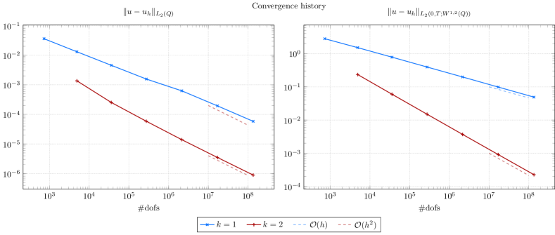
Figure 1: Example 5.1 ($d=2$): Convergence history of the discretization errors in different norms for linear ($k=1$) and quadratic ($k=2$) shape functions.

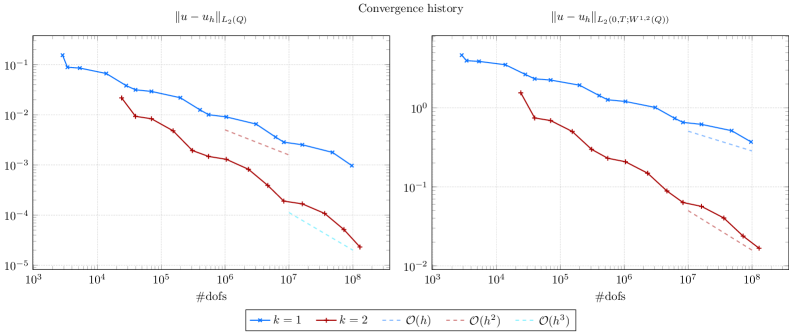
Figure 2: Example 5.1 ($d=3$): Convergence history of the discretization errors in different norms for linear ($k=1$) and quadratic ($k=2$) shape functions.

Finally, we study the performance of the nested Newton solver. As already mentioned earlier, we can solve the linear systems arising in Newton’s method by means of a sparse direct solver, or by means of an iterative method, e.g., the preconditioned GMRES method. The preconditioner is constructed by algebraic multigrid (AMG), where we use a standard V-cycle with one pre- and one post-smoothing step; cf. [36, 64]. Moreover, we will numerically investigate the influence of the regularization parameter $\varepsilon$ on the solution process. In Table 1, we present scaling results wrt uniform mesh refinement. Here, we can observe that the regularization parameter has only a mild influence on Newton’s method, but does affect the convergence behaviour of the inner GMRES solver; compare, e.g., the total number of GMRES iterations in brackets for refinement level $\ell=3$ in Table 1.

Table 1: Example 5.1: Scaling of the (damped) Newton solver with total number of inner solves in brackets, for $d+1=3$ and $k=1$; using 256 cores of HPC Cluster RADON1.

$\ell$	$\#\mathrm{dofs}$	$\varepsilon=1$			$\varepsilon=10^{-5}$			$\varepsilon=10^{-10}$
		GMRES		MUMPS	GMRES		MUMPS	GMRES		MUMPS
0	$4913$	$11$	($322$)	$11$	$12$	($370$)	$12$	$12$	($370$)	$12$
1	$35\,937$	$3$	($70$)	$3$	$3$	($185$)	$3$	$3$	($185$)	$3$
2	$274\,625$	$2$	($62$)	$2$	$2$	($200$)	$2$	$2$	($200$)	$2$
3	$2\,146\,689$	$2$	($87$)	–	$6$	($600$)	–	$6$	($600$)	$6$
4	$16\,974\,593$	$2$	($137$)	–	$4$	($400$)	–	$4$	($400$)	–
5	$135\,005\,697$	$2$	($200$)	–	$3$	($300$)	–	$3$	($300$)	–

5.2 Goal-oriented Adaptivity Driven by a Linear Functional

Next, we consider the same setting as in the previous Example 5.1. However, we are now not interested in behaviour of the solution $u$ in the complete space-time cylinder $Q$, but only in the integral over the spatial domain $\Omega$ at final time $T$, i.e. we are interested in the goal functional

$$J(u)=\int_{\Omega}\!u(\,.\,,T)\;\mathrm{d}\Omega.$$

Since the exact solution $u$ is given by (20), we can compute the value of the goal functional

$$J(u)=\frac{4\,e}{\pi^{2}}\approx 1.10167812933171$$

at the exact solution $u$.

Let us first consider the convergence history of the error in the linear functional $J(\cdot)$ for $d=2$; see the left plot of Figure 3. Here we observe that uniform refinements result in an error rate of $O(h)$, where the mesh parameter $h$ is defined as $h=N_{h}^{-1/d}$, with $N_{h}$ the total number of space-time dofs. On the other hand, using adaptive refinements driven by the goal-oriented error estimator, we obtain an improved rate of $O(h^{1.7})$. Moreover, we also take a look at the efficiency index $\mathrm{I_{eff}}$ of the error estimator; cf. the right plot of Figure 3. We observe that, after some initial oscillations, the efficiency index for the adaptive refinements remains close to $1$. Figure 4 shows that the same observations can be made in case $d=3$, where the space-time cylinder $Q\subset\mathbb{R}^{4}$.

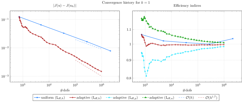
Figure 3: Example 5.2 ($d=2$): Convergence history of the error in the functional as well as efficiency plots, where we additionally included the efficiency of the primal and adjoint parts, respectively.

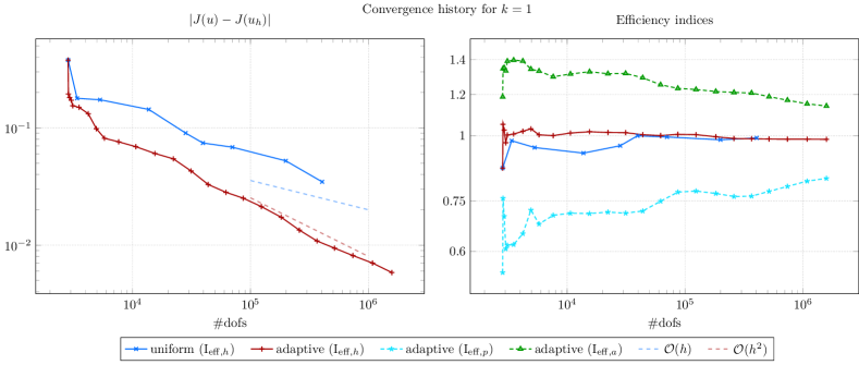
Figure 4: Example 5.2 ($d=3$): Convergence history of the error in the functional as well as efficiency plots, where we additionally included the efficiency of the primal and adjoint parts, respectively.

Next, let us consider the meshes produced by the adaptive finite element method. Since our quantity of interest is concentrated at the final time $T$, we expect heavy refinements towards the top of the space-time cylinder $Q$. In Figure 5, we present the initial mesh as well as the mesh after a certain number of adaptive refinements for the case $d=2$. Indeed, as we can observe in the lower row of Figure 5, the mesh refinements are concentrated

towards the top $\Sigma_{T}$ of the space-time cylinder $Q$. This behaviour is also visible if we cut the space-time cylinder $Q$ along the $(x_{2},t)$-plane at $x_{1}=0.5$; cf. the lower right plot of Figure 5. The refinements seem to be entirely concentrated in the final quarter of the time interval $(0,T)$. This rather broad refinement is due to the mesh refinement algorithms that on the one hand isotropically refine each simplex, and on the other hand also refine the neighborhood of an element in order to prevent mesh degeneration.

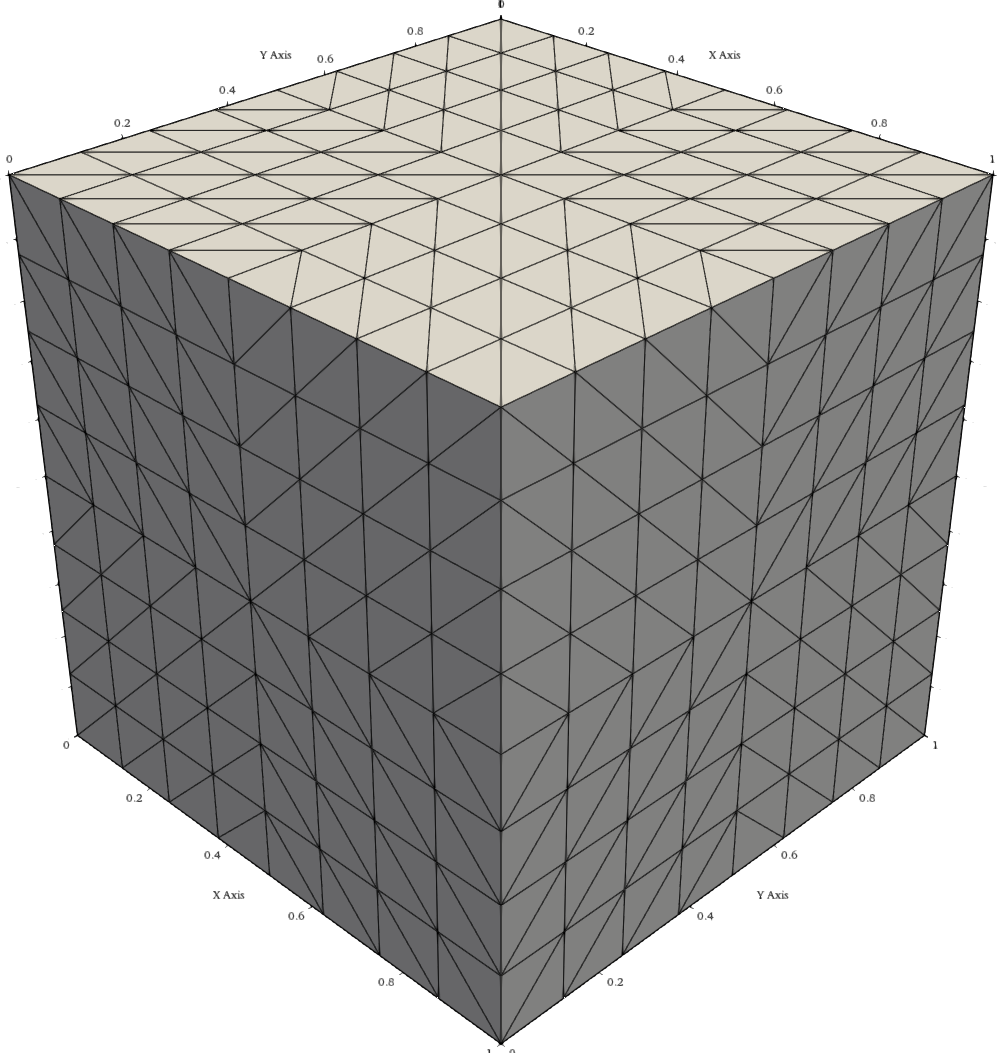
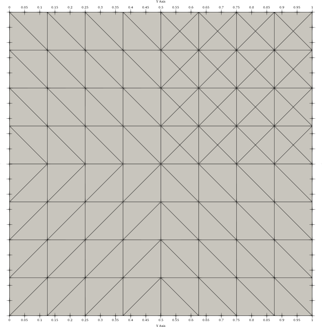
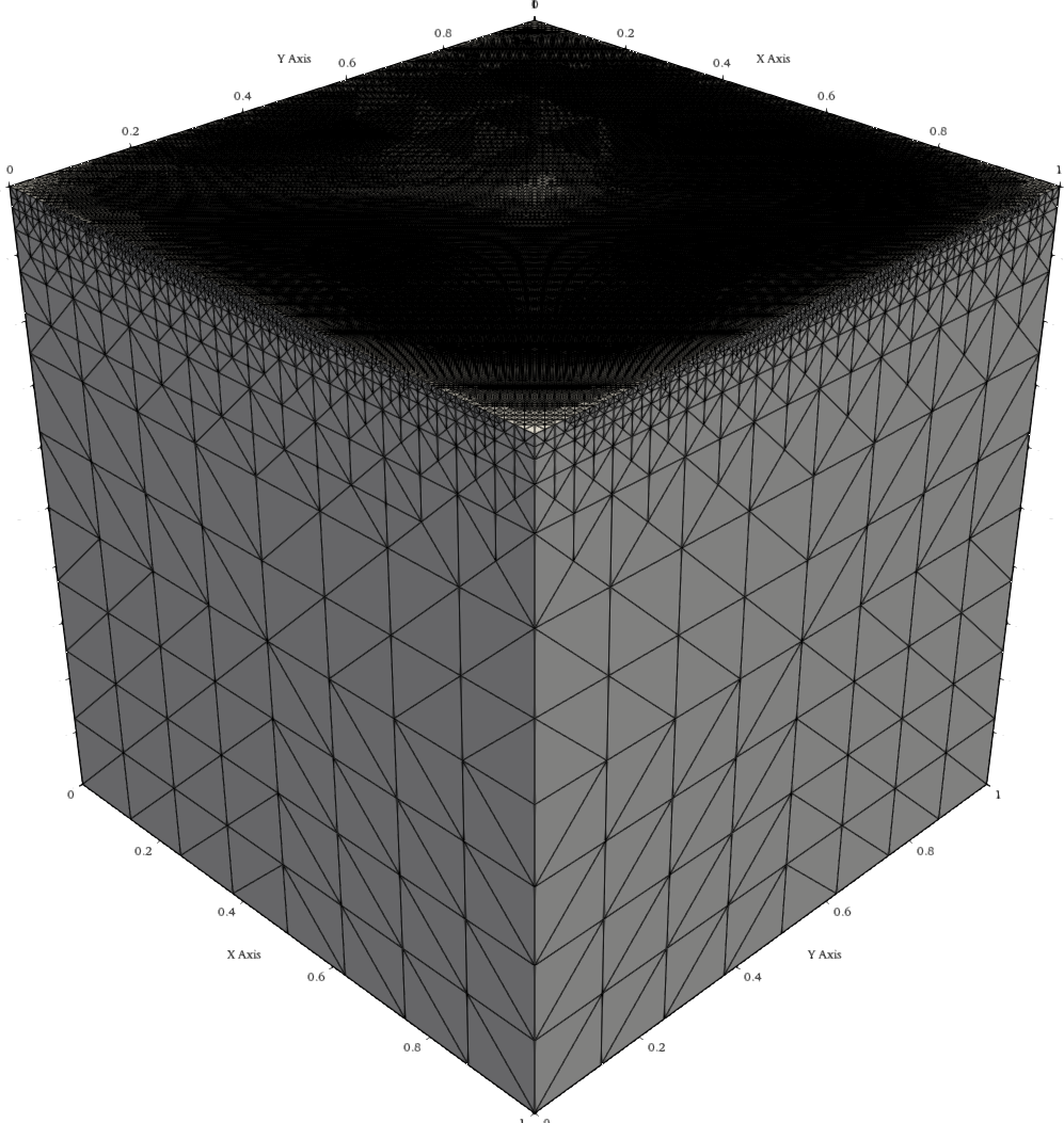
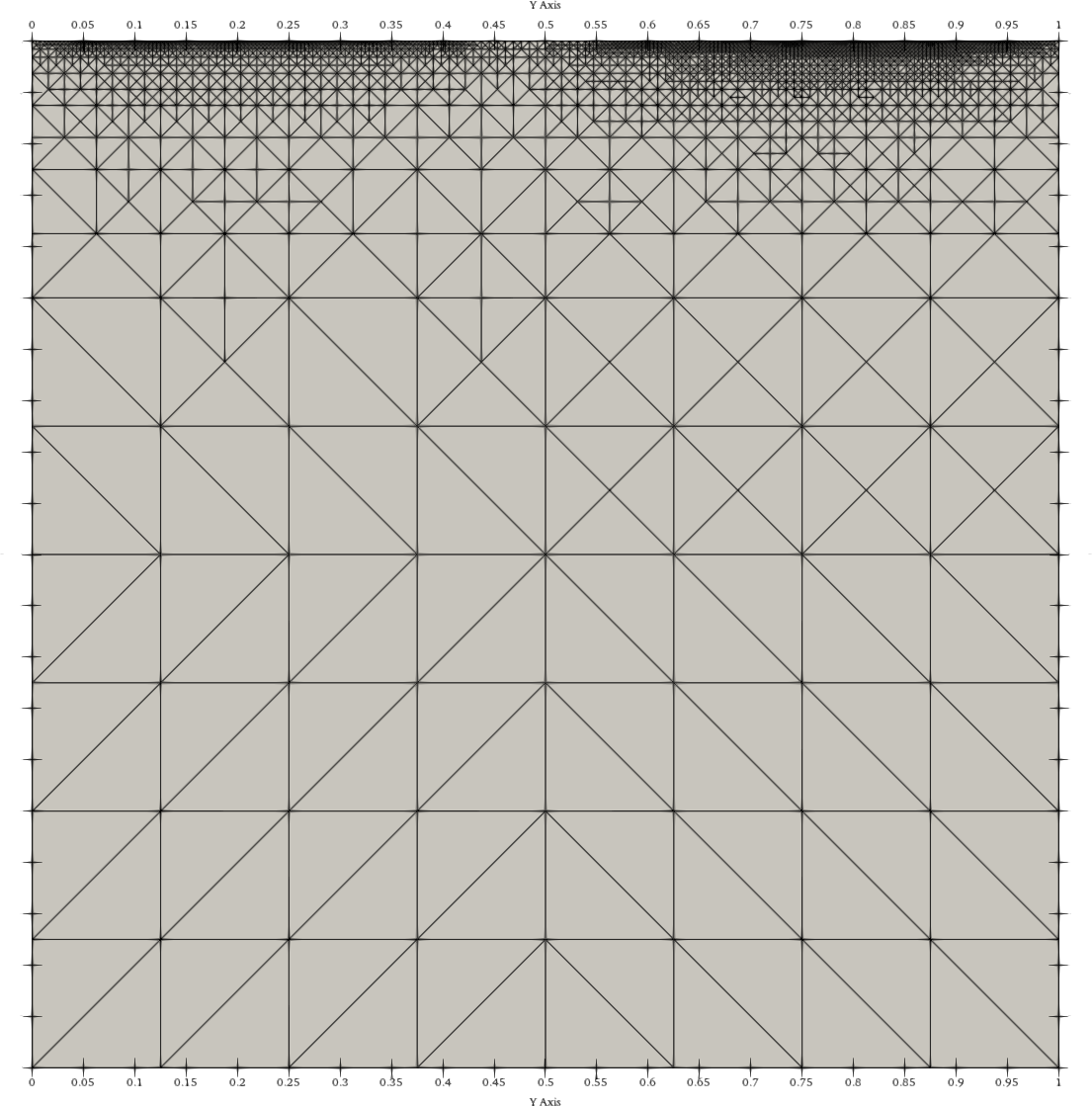
Figure 5: Example 5.2 ($d=2$): Initial space-time mesh (upper left); $(x_{2},t)$-plane at $x_{1}=0.5$ of the initial space-time mesh (upper right); space-time mesh after 45 adaptive refinements (lower left); $(x_{2},t)$-plane at $x_{1}=0.5$ after 45 adaptive refinements (lower right); using linear finite elements.

Let us once more consider the performance of the nested Newton method. As for the previous Example 5.1, we investigate the influence of the regularization parameter $\varepsilon$, the inner solver, and the adaptive meshes on the solution process. In Table 2, we present the scaling with respect to the adaptive refinement levels $\ell$ for different regularization parameters $\varepsilon$. At a first glance, the damped Newton’s method seems rather robust wrt the parameters.

Table 2: Example 5.2: Scaling of the (damped) Newton solver with total number of inner solves in brackets, for $d+1=3$ and $k=1$.

$\ell$	$\#\mathrm{dofs}$	$\varepsilon=1$			$\varepsilon=10^{-5}$			$\varepsilon=10^{-10}$
		GMRES		MUMPS	GMRES		MUMPS	GMRES		MUMPS
$0$	$\sim 729$	$9$	($170$)	$9$	$11$	($231$)	$11$	$11$	($231$)	$11$
$12$	$\sim 4346$	$3$	($112$)	$3$	$3$	($171$)	$3$	$3$	($171$)	$3$
$20$	$\sim 33\,886$	$2$	($156$)	$2$	$2$	($200$)	$2$	$2$	($200$)	$2$
$28$	$\sim 264\,942$	$2$	($200$)	$2$	$2$	($200$)	$3$	$2$	($200$)	$3$
$34$	$\sim 1\,112\,168$	$2$	($200$)	–	$2$	($200$)	–	$2$	($200$)	–

5.3 Goal-Oriented with a Non-linear Goal Functional

As our third example, we consider again the setting from the previous two examples. However, we are now interested in the following, non-linear volume goal functional

$$J(u)=\int_{Q_{I}}\!|\nabla_{x}u|^{p}\;dQ\approx 0.01937125060566419,$$

where $Q_{I}$ is a prescribed region of interest. In our case, we choose $Q_{I}$ to be an octahedron with edge length $0.5$, centered at $(0.5,0.5,0.5)$; see also the middle column of Figure 7. We make this choice in order to exactly capture the region of interest with the finite element mesh.

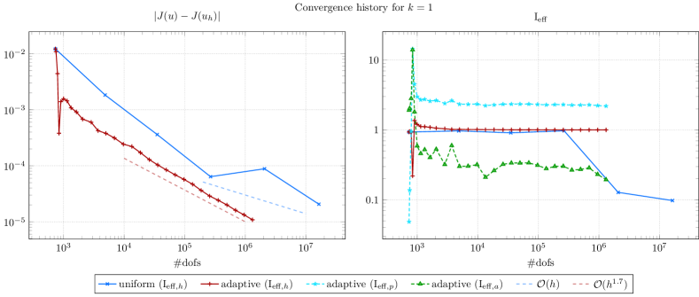
Figure 6: Example 5.3 ($d=2$): Convergence history of the error in the functional as well as efficiency plots, where we additionally included the efficiency of the primal and adjoint parts, respectively.

Let us first consider the convergence history. In the left plot Fig. 6, we present the convergence history of the discretization error in the nonlinear goal functional $J(u)$. We observe that while uniform refinements reduce the overall error, adaptive refinements driven by the goal oriented error estimator lead to a considerable reduction in the number of dofs needed to attain a similar error. Moreover, we observe that the efficiency index of the adaptive refinements once more converges towards $1$; cf. the right plot of Fig. 6.

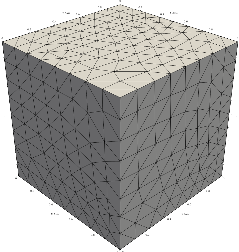
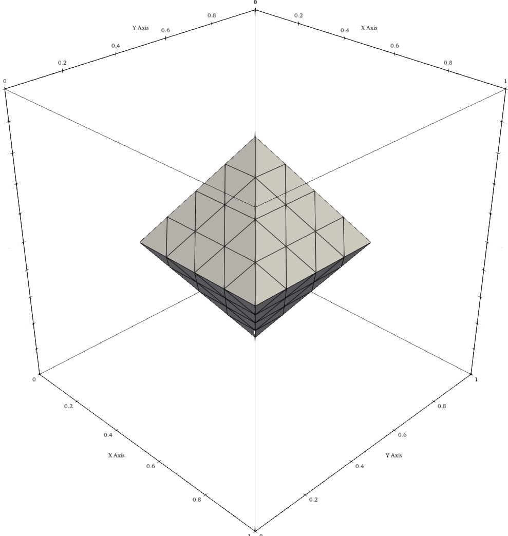
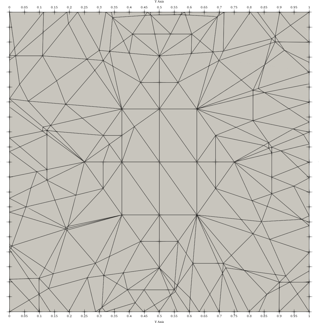
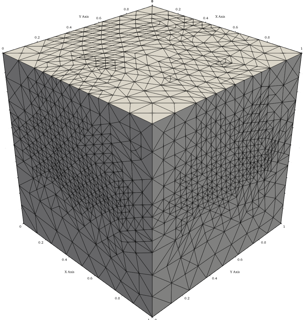
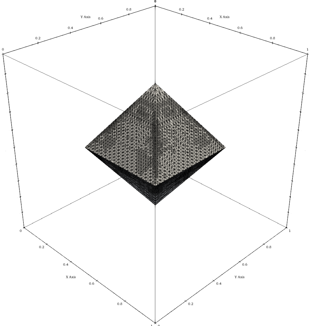
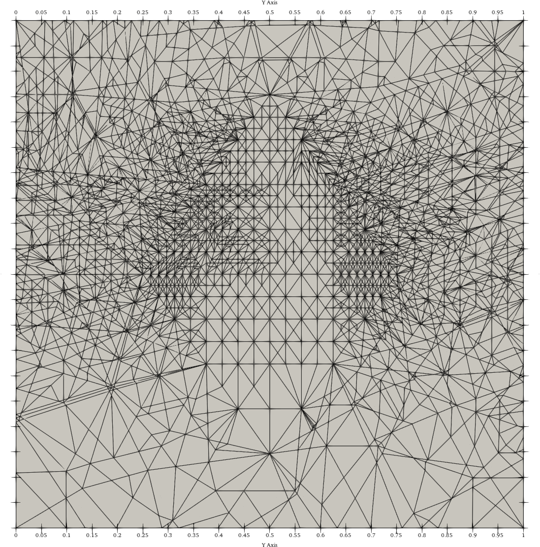
Figure 7: Example 5.3 ($d=2$): From left to right: full space-time mesh, surface mesh of $Q_{I}$, and the $(x_{2},t)$-plane at $x_{1}=0.5$; in its initial configuration (upper row), and after 20 adaptive refinements (lower row); using linear finite elements.

The upper row of Figure 7 presents the initial configuration of the finite element meshes, whereas the lower row shows the meshes after 20 adaptive refinements driven by the goal oriented estimator. In the very left column, we can observe that the adaptive refinement indeed produces mostly unstructured space-time mesh. Moreover, we see that the refinements are concentrated inside the octahedron $Q_{I}$, and any refinements outside are necessary in order to avoid any degeneration of the mesh elements.

In Table 3, we again present the scaling wrt the level of refinement $\ell$ of the nested Newton method for different regularization parameters $\varepsilon$. We again observe stable iteration counts between two and three Newton iterations as well as increasing iteration counts for the total number of inner solves for the Jacobian.

Table 3: Example 5.3: Scaling of the (damped) Newton solver with total number of inner solves in brackets, for $d+1=3$ and $k=1$.

$\ell$	$\#\mathrm{dofs}$	$\varepsilon=1$			$\varepsilon=10^{-5}$			$\varepsilon=10^{-10}$
		GMRES		MUMPS	GMRES		MUMPS	GMRES		MUMPS
$0$	$\sim 735$	$10$	($199$)	$10$	$11$	($240$)	$11$	$11$	($240$)	$11$
$8$	$\sim 4931$	$3$	($81$)	$3$	$3$	($104$)	$3$	$3$	($104$)	$3$
$15$	$\sim 56\,031$	$2$	($92$)	$2$	$2$	($160$)	$2$	$2$	($160$)	$2$
$18$	$\sim 155\,318$	$2$	($114$)	$2$	$2$	($200$)	$3$	$2$	($200$)	$3$
$24$	$\sim 1\,133\,165$	$2$	($200$)	–	$3$	($300$)	–	$3$	($300$)	–

6 Conclusion and Outlook

We have proposed a new goal-oriented adaptive space-time finite element method for regularized parabolic $p$-Laplace initial-boundary value problems. The space-time finite element discretization is based on the decomposition of the space-time cylinder into conforming simplicial elements like in the case of elliptic boundary value problems. The mesh refinement is driven by the DWR method and their localization is done by means of the PU technique. So we can adaptively generate finite element approximations that are tailored to the quantity of interest (goal) that is mathematically given by some possibly nonlinear functional. Since we used a manufactured solution in our numerical experiments, we were able to compute the efficiency indices as quotient of the estimated error and the real error of the approximations to the functional. In all cases the efficiency indices were close to one. The adaptive process always saved a lot of unknowns in order to obtain some accuracy in the approximation of the functional in comparison with uniform refinement. However, at each refinement level, we have to solve one non-linear system for the finite element solution and one linear linear system for the adjoint finite element solution. Furthermore, we need improved approximations to primal and adjoint solutions that can be obtained by different methods as discussed in Subsection 4.2.

A priori discretization error estimates as were proved in the case of linear parabolic initial-boundary value problem [59], convergence analysis of the adaptive process, investigation of the convergence of the Newton solver, improvement of the inner solver respectively preconditioner for the Jacobian system at each Newton iteration step, and the adaption of the inner iteration to the convergence of the Newton iteration are future research topics. The latter topic as well as the simultaneous parallelization in space and time can lead to a considerably improvement of the performance of the algorithm. This is also important for more complex practical applications like non-Newtonian flow problems described by power law models; see e.g. [63] and the references therein.

References

- [1] K. Ahuja, B. Endtmayer, M. C. Steinbach, and T. Wick. Multigoal-oriented error estimation and mesh adaptivity for fluid–structure interaction. J. Comput. Appl. Math., 412:114315, 2022.
- [2] J. Alvarez-Aramberri, D. Pardo, and H. Barucq. Inversion of magnetotelluric measurements using multigoal oriented hp-adaptivity. Procedia Comput. Sci., 18:1564 – 1573, 2013.
- [3] P. Amestoy, I. Duff, J.-Y. L’Excellent, and J. Koster. Mumps: A general purpose distributed memorysparse solver. In T. Sørevik, F. Manne, R. Moe, and A. Gebremedhin, editors, AppliedParallel Computing: New Paradigms for HPCin Industry and Academia, volume 1947 of Lecture Notes in Computer Science. Springer-Verlag, Berlin, Heidelberg, 2001.
- [4] R. Anderson, J. Andrej, A. Barker, J. Bramwell, J.-S. Camier, J. C. V. Dobrev, Y. Dudouit, A. Fisher, T. Kolev, W. Pazner, M. Stowell, V. Tomov, I. Akkerman, J. Dahm, D. Medina, and S. Zampini. MFEM: A modular finite element methods library. Comput. Math. Appl., 81:42–74, 2021.
- [5] S. Balay, S. Abhyankar, M. F. Adams, S. Benson, J. Brown, P. Brune, K. Buschelman, E. Constantinescu, L. Dalcin, A. Dener, V. Eijkhout, J. Faibussowitsch, W. D. Gropp, V. Hapla, T. Isaac, P. Jolivet, D. Karpeev, D. Kaushik, M. G. Knepley, F. Kong, S. Kruger, D. A. May, L. C. McInnes, R. T. Mills, L. Mitchell, T. Munson, J. E. Roman, K. Rupp, P. Sanan, J. Sarich, B. F. Smith, S. Zampini, H. Zhang, H. Zhang, and J. Zhang. PETSc/TAO users manual. Technical Report ANL-21/39 - Revision 3.18, Argonne National Laboratory, 2022.
- [6] W. Bangerth and R. Rannacher. Adaptive Finite Element Methods for Differential Equations. Birkhäuser Verlag, Boston, 2003.
- [7] J. Barrett and W. Lui. Finite element approximation of the parabolic -Laplacian. SIAM J. Numer. Analy., 31(2):413–428, 1994.
- [8] R. Becker, V. Heuveline, and R. Rannacher. An optimal control approach to adaptivity in computational fluid mechanics. Int. J. Numer. Methods Fluids, 40(1-2):105–120, 2002.
- [9] R. Becker and R. Rannacher. Weighted a posteriori error control in FE methods. In Lecture ENUMATH-95, Paris, Sept. 18-22, 1995, in: Proc. ENUMATH-97, Heidelberg, Sept. 28 - Oct.3, 1997 (H.G. Bock, et al., eds). pp. 621–637, World Sci. Publ., Singapore, 1998.
- [10] R. Becker and R. Rannacher. An optimal control approach to a posteriori error estimation in finite element methods. Acta Numer., 10:1–102, 2001.
- [11] S. Beuchler, B. Endtmayer, J. Lankeit, and T. Wick. Multigoal-oriented a posteriori error control for heated material processing using a generalized Boussinesq model. Comptes Rendus. Mécanique, Special Issue in Honor of Roland Glowinski, 2023. Online first.
- [12] S. Beuchler, B. Endtmayer, and T. Wick. Goal oriented error control for stationary incompressible flow coupled to a heat equation. PAMM, 21(1):e202100151, 2021.
- [13] H. Blum, A. Schröder, and F.-T. Suttmeier. A posteriori estimates for fe-solutions of variational inequalities. In Numerical Mathematics and Advanced Applications, pages 669–680. Springer, 2003.
- [14] M. Braack and A. Ern. A posteriori control of modeling errors and discretization errors. Multiscale Model. Simul., 1(2):221–238, 2003.
- [15] S. C. Brenner and L. R. Scott. The mathematical theory of finite element methods, volume 15 of Texts in Applied Mathematics. Springer, New York, third edition, 2008.
- [16] M. P. Bruchhäuser, K. Schwegler, and M. Bause. Numerical study of goal-oriented error control for stabilized finite element methods. In Chemnitz Fine Element Symposium, pages 85–106. Springer, 2017.
- [17] A. Cianchi and V. Maz’ya. Second-order regularity for parabolic -laplace problems. J. Geom. Anal., 30:1565–1583, 2020.
- [18] T. Davis. Direct methods for sparse linear system. SIAM, Philadelphia, 2006.
- [19] P. Deuflhard. Newton Methods for Nonlinear Problems, volume 35 of Springer Series in Computational Mathematics. Springer Berlin Heidelberg, 2011.
- [20] J. I. Dıaz. Nonlinear Partial Differential Equations and Free Boundaries. Pitman Advanced Publishing Program, Boston-London-Melbourne, 1985.
- [21] E. DiBenedetto. Degenerate Parabolic Equations. Springe, New York, 1993.
- [22] V. Dolejší, O. Bartoš, and F. Roskovec. Goal-oriented mesh adaptation method for nonlinear problems including algebraic errors. Comput. Math. Appl., 93:178–198, 2021.
- [23] W. Dörfler. A convergent adaptive algorithm for Poisson’s equation. SIAM J. Numer. Anal., 33(3):1106–1124, 1996.
- [24] B. Endtmayer. Multi-goal oriented a posteriori error estimates for nonlinear partial differential equations. PhD thesis, Johannes Kelper University Linz, 2020. Available at: https://epub.jku.at/obvulihs/download/pdf/5767444.
- [25] B. Endtmayer, A. Demircan, D. Perevoznik, U. Morgner, S. Beuchler, and T. Wick. Adaptive finite element simulations of laser-heated material flow using a boussinesq model. PAMM, 23(1):e202200219, 2023.
- [26] B. Endtmayer, U. Langer, I. Neitzel, T. Wick, and W. Wollner. Multigoal-oriented optimal control problems with nonlinear PDE constraints. Comput. Math. Appl., 79(10):3001–3026, 2020.
- [27] B. Endtmayer, U. Langer, J. P. Thiele, and T. Wick. Hierarchical DWR error estimates for the Navier-Stokes equations: h and p enrichment. In Numerical Mathematics and Advanced Applications ENUMATH 2019, pages 363–372. Springer, 2021.
- [28] B. Endtmayer, U. Langer, and T. Wick. Multigoal-oriented error estimates for non-linear problems. J. Numer. Math., 27(4):215–236, 2019.
- [29] B. Endtmayer, U. Langer, and T. Wick. Two-Side a Posteriori Error Estimates for the Dual-Weighted Residual Method. SIAM J. Sci. Comput., 42(1):A371–A394, 2020.
- [30] B. Endtmayer and T. Wick. A Partition-of-Unity Dual-Weighted Residual Approach for Multi-Objective Goal Functional Error Estimation Applied to Elliptic Problems. Comput. Methods Appl. Math., 17(4):575–599, 2017.
- [31] A. Ern and J.-L. Guermond. Theory and Practice of Finite Elements. Springer-Verlag, New York, 2004.
- [32] M. Feischl, D. Praetorius, and K. G. van der Zee. An abstract analysis of optimal goal-oriented adaptivity. SIAM J. Numer. Anal., 54(3):1423–1448, 2016.
- [33] P. Fick, E. Brummelen, and K. Zee. On the adjoint-consistent formulation of interface conditions in goal-oriented error estimation and adaptivity for fluid-structure interaction. Comput. Methods Appl. Mech. Engrg., 199(49-52):3369–3385, 2010.
- [34] H. Fischer, J. Roth, T. Wick, L. Chamoin, and A. Fau. MORe DWR: Space-time goal-oriented error controlfor incremental POD-based ROM. Available at SSRN 4420888, 2023.
- [35] B. N. Granzow, D. T. Seidl, and S. D. Bond. Linearization errors in discrete goal-oriented error estimation. arXiv preprint arXiv:2305.15285, 2023.
- [36] W. Hackbusch. Multi-Grid Methods and Applications, volume 4 of Springer Series in Computational Mathematics. Springer-Verlag, Berlin, Heidelberg, 1985.
- [37] R. Hartmann. Multitarget error estimation and adaptivity in aerodynamic flow simulations. SIAM J. Sci. Comput., 31(1):708–731, 2008.
- [38] R. Hartmann and P. Houston. Goal-oriented a posteriori error estimation for multiple target functionals. In Hyperbolic problems: theory, numerics, applications, pages 579–588. Springer, Berlin, 2003.
- [39] A. Hirn and W. Wollner. An optimal control problem for equations with -structure and its finite element discretization. In R. Herzog, M. Heinkenschloss, D. Kalise, G. Stadler, and E. Trélat, editors, Optimization and Control for Partial Differential Equations, volume 29 of Radon Series on Computational and Applied Mathematics, chapter 7, pages 137–166. De Gruyter, 2022.
- [40] A. Kaltenbach. Error analysis for a crouzeix-raviart approximation of the -dirichlet problem. arXiv preprint arXiv:2210.12116, 2022.
- [41] K. Kergrene, S. Prudhomme, L. Chamoin, and M. Laforest. A new goal-oriented formulation of the finite element method. Comput. Methods Appl. Mech. Engrg., 327:256–276, 2017.
- [42] U. Köcher, M. P. Bruchhäuser, and M. Bause. Efficient and scalable data structures and algorithms for goal-oriented adaptivity of space–time FEM codes. SoftwareX, 10:100239, 2019.
- [43] U. Langer, M. Neumüller, and A. Schafelner. Space-time finite element methods for parabolic evolution problems with variable coefficients. In T. Apel, U. Langer, A. Meyer, and O. Steinbach, editors, Advanced Finite Element Methods with Applications - Selected Papers from the 30th Chemnitz Finite Element Symposium 2017, volume 128 of Lecture Notes in Computational Science and Engineering (LNCSE), chapter 13, pages 229–256. Springer, Berlin, Heidelberg, New York, 2019.
- [44] U. Langer and A. Schafelner. Adaptive space-time finite element methods for non-autonomous parabolic problems with distributional sources. Comput. Methods Appl. Math., 20(4):677–693, 2020.
- [45] U. Langer and A. Schafelner. Simultaneous space-time finite element methods for parabolic optimal control problems. In International Conference on Large-Scale Scientific Computing, pages 314–321. Springer, 2021.
- [46] U. Langer and A. Schafelner. Adaptive space–time finite element methods for parabolic optimal control problems. J. Numer. Math., 30(4):247–266, 2022.
- [47] U. Langer, O. Steinbach, F. Tröltzsch, and H. Yang. Unstructured space-time finite element methods for optimal control of parabolic equation. SIAM J. Sci. Comput., 43(2):A744–A771, 2021.
- [48] Y.-J. Lee and J. Park. On the linear convergence of additive Schwarz methods for the -Laplacian. arXiv preprint arXiv:2210.09183, 2022.
- [49] J.-L. Lions. Quelques méthodes de résolution des problèmes aux limites non linéaires. Dunod Gauthier-Villars, Paris, 1969.
- [50] G. Mallik, M. Vohralik, and S. Yousef. Goal-oriented a posteriori error estimation for conforming and nonconforming approximations with inexact solvers. J. Comput. Appl. Math., 366, 07 2019.
- [51] MFEM: Modular finite element methods [Software]. mfem.org.
- [52] R. Rannacher and J. Vihharev. Adaptive finite element analysis of nonlinear problems: balancing of discretization and iteration errors. J. Numer. Math., 21(1):23–61, 2013.
- [53] T. Richter and T. Wick. Variational localizations of the dual weighted residual estimator. J. Comput. Appl. Math., 279:192–208, 2015.
- [54] J. Roth, J. P. Thiele, U. Köcher, and T. Wick. Tensor-product space-time goal-oriented error control and adaptivity with partition-of-unity dual-weighted residuals for nonstationary flow problems. arXiv preprint arXiv:2210.02965, 2022.
- [55] T. Roubíc̆ek. Nonlinear Partial Differential Equations with Applications, volume 153 of International Series of Numerical Mathematics. Springer, Basel, second edition, 2013.
- [56] Y. Saad. Iterative Methods for Sparse Linear Systems. SIAM, Philadelphia, 2003.
- [57] A. Schafelner. Space-time finite element methods. PhD thesis, Johannes Kelper University Linz, 2022. Available at: https://epub.jku.at/obvulihs/download/pdf/7306528.
- [58] O. Steinbach. Numerical Approximation Methods for Elliptic Boundary Value Problems: Finite and Boundary Elements. Springer, 2008.
- [59] O. Steinbach. Space-time finite element methods for parabolic problems. Comput. Methods Appl. Math., 15(4):551–566, 2015.
- [60] O. Steinbach and H. Yang. Space-time finite element methods for parabolic evolution equations: discretization, a posteriori error estimation, adaptivity and solution. In Space-Time Methods: Application to Partial Differential Equations, volume 25 of Radon Series on Computational and Applied Mathematics, chapter 7, pages 207–248. de Gruyter, Berlin, 2019.
- [61] R. Stevenson. The completion of locally refined simplicial partitions created by bisection. Math. Comp., 77(261):227–241, 2008.
- [62] I. Toulopoulos. Numerical solutions of quasilinear parabolic problems by a continuous space-time finite element scheme. SIAM J. Sci. Comput., 44(5):A2944–A2973, 2022.
- [63] I. Toulopoulos. A unified time discontinuous Galerkin space-time finite element scheme for non-Newtonian power law models. Int. J. Numer. Methods Fluids, 2022. published first online, doi.org/10.1002/fld.5170.
- [64] U. Trottenberg, C. Oosterlee, and A. Schüller. Multigrid. Academic Press, London, 2001.
- [65] E. Zeidler. Nonlinear Functional Analysis and its Applications II/B: Nonlinear Monotone Operators. Springer, New York, 1990.