Painlevé transcendents in the defocusing mKdV equation with non-zero boundary conditions

Abstract

We consider the Cauchy problem for the defocusing modified Korteweg-de Vries (mKdV) equation with non-zero boundary conditions

$$q_{t}(x,t)-6q^{2}(x,t)q_{x}(x,t)+q_{xxx}(x,t)=0,$$

$$q(x,0)=q_{0}(x)\to\pm 1,\ \ x\rightarrow\pm\infty,$$

which can be characterized using a Riemann-Hilbert (RH) problem through the inverse scattering transform. Using the $\bar{\partial}$ generalization of the Deift-Zhou nonlinear steepest descent approach, combined with the double scaling limit technique, we obtain the long-time asymptotics of the solution of the Cauchy problem in the transition region $|x/t+6|t^{2/3}<C$ with $C>0$. The asymptotics is expressed in terms of the solution of the second Painlevé transcendent.

1 Introduction

This paper is concerned with the Painlevé asymptotics of the defocusing modified Korteweg-de Vries (mKdV) equation with non-zero boundary conditions

$$q_{t}(x,t)-6q^{2}(x,t)q_{x}(x,t)+q_{xxx}(x,t)=0,$$ (1.1)

$$q(x,0)=q_{0}(x)\to\pm 1,\ \ x\rightarrow\pm\infty,$$ (1.2)

where $q_{0}\in\tanh(x)+H^{4,4}(\mathbb{R})$. The mKdV equation arises in various of physical fields, such as acoustic wave and phonons in a certain anharmonic lattice [1, 2], Alfvén wave in a cold collision-free plasma [3, 4]. The mKdV equation on the line are locally well-posed [5] and globally well-posed in $H^{s}(\mathbb{R})$ for $s\geq\frac{1}{4}$ [6, 7, 8]. Recently, the global well-posedness to the Cauchy problem for the mKdV equation was further generalized to the space $H^{s}(\mathbb{R})$ for $s>-\frac{1}{2}$ [9].

It is well-established that the defocusing mKdV equation (1.1) with zero boundary conditions (ZBCs, i.e., $q_{0}(x)\rightarrow 0$ as $x\rightarrow\pm\infty$), does not exhibit solitons due to the absence of discrete spectrum in the self-adjoint ZS-AKNS scattering operator (see (2.1) below) [10]. Numerous studies have been conducted to analyze the long-time asymptotic behavior of solutions to the equation (1.1) in the continuous spectrum without solitons. The earliest work can be traced back to Segur and Ablowitz [11], who derived the leading asymptotics of the solution of the mKdV equation, including the full information on the phase. The Deift-Zhou method [10] has significantly influenced research on the long-time behavior of the mKdV equation (1.1), rigorously deriving the asymptotics for all relevant regions, including the self-similar Painlevé region, under the conditions of soliton free. The long-time asymptotic behavior of the solution of the mKdV equation with step-like initial data has been extensively studied in previous works [12, 13, 14, 15, 16]. Boutet de Monvel et al. discussed the initial boundary value problem of the defocusing mKdV equation in the finite interval using the Fokas method [17]. Moreover, the long-time behavior of solutions to the defocusing mKdV equation (1.1) was established for initial data in a weighted Sobolev space $H^{2,2}(\mathbb{R})$ without considering solitons [18]. Furthermore, Charlier and Lenells investigated the Airy and Painlevé asymptotics for the mKdV equation [19], and Painlevé asymptotics were later obtained for the entrie mKdV hierarchy by Huang and Zhang [20]. The Painlevé asymptotics in transition regions also appear in the other integrable systems. Segur and Ablowitz first described the asymptotics in the transition region for the Korteweg-de Vries (KdV) equation [11]. The connection between the tau-function of the Sine-Gordon reduction and the Painlevé III equation was established through the RH approach [21]. Additionally, Boutet de Monvel et al. found the Painlevé asymptotics of the Camassa-Holm equation using the nonlinear steepest descent approach [22]. More recently, we found the Painlevé asymptotics of the defocusing nonlinear Schrödinger (NLS) equation with non-zero boundary conditions (NBCs, i.e., $q_{0}(x)\nrightarrow 0$ as $x\rightarrow\pm\infty$) [23].

However, it is worth noting that the defocusing mKdV equation (1.1) with NBCs (1.2) allows the existence of solitons due to the presence of a non-empty discrete spectrum. The corresponding $N$-soliton solutions were skillfully constructed using the inverse scattering transform (IST) [24]. Recently, by using $\bar{\partial}$ steepest descent method, which was introduced in [25, 26] and has been extensively implemented in the long-time asymptotic analysis and soliton resolution conjecture of integrable systems [27, 28, 29, 30, 31, 32], the long-time asymptotics of the solution to the Cauchy problem (1.1)-(1.2) was obtained in two regions: a solitonic region $-6<\xi\leq-2$ (where $\xi:=x/t$) [33] and a solitonless region $\{\xi<-6\}\cup\{\xi>-2\}$ [34] respectively (See Figure 1). The remaining question is: How to describe the asymptotics of the solution to the Cauchy problem (1.1)-(1.2) in the transition region $\xi\approx-6$?

In this paper, we demonstrate that the long-time asymptotics of the solution to the Cauchy problem (1.1)-(1.2) in this transition region can be expressed in terms of the solution of the Painlevé II equation. In the generic case of the mKdV equation, the norm $(1-|r(z)|^{2})^{-1}$ blows up as $z\to\pm 1$. This is not merely a technical difficulty, but indicates the emergence of a new phenomenon that cannot be treated in the same manner as the cases in [33, 34]. In the context of our research, we confirm the Painlevé asymptotics in the transition region $\xi\approx-6$. Compared with the case of ZBCs [10, 19, 20], the case of NZBCs we considered meets substantial difficulties. Firstly, due to the effect of solitons on the Cauchy problem (1.1)-(1.2), a more detailed description is necessary to formulate a solvable model. Secondly, in the case of the mKdV equation (1.1) with ZBCs, the phase function is given by

$$\theta(z)=2z^{3}+zx/t,$$

and the corresponding RH problem can directly match a Painlevé II RH problem (see A) [10, 19, 20]. However, in the case of NBCs (1.1)-(1.2), the phase function becomes

$$\theta(z)=\lambda(z)\left(x/t+4k^{2}(z)+2\right),$$

and the corresponding RH problem cannot directly match the Painlevé II RH problem. To confront this difficulty, we propose a key technique to approximate the phase function of the Painlevé II RH problem using double series (see (4.25)-(4.26) below).

Figure 1: The $(x,t)$-plane is divided into three kinds of asymptotic regions: Solitonic region, $-6<\xi\leq-2$; Solitonless region, $\xi<-6$ and $\xi>-2$; Transition region, $\xi\approx-6$.

The organization of the present paper is as follows: In Section 2, we consider the forward scattering transform for the Cauchy problem (1.1)-(1.2), including the properties of the Jost functions and the scattering data derived from the initial data. In Section 3, we perform the inverse scattering transform and establish a matrix-valued RH problem associated with the Cauchy problem. Furthermore, we transform the original RH problem to a regular RH problem, removing the effect of solitons and the spectral singularities. In Section 4, we investigate the Painlevé asymptotics in the transition region $\left|\frac{x}{t}+6\right|t^{2/3}<C$ for any $C>0$. The $\bar{\partial}$ steepest descent approach and the double scaling limit technique are applied to deform the regular RH problem into a solvable RH model that matches with the Painlevé II RH problem. Following the analysis presented in the preceding sections, we establish the main result on the Painlevé asymptotics (see Theorem 4.10).

Remark 1.1.

For the generic case when $|r(\pm 1)|=1$, Cuccagna and Jenkins proposed a new way in [35] to get rid of the restrictive condition $\|r\|_{L^{\infty}(\mathbb{R})}<1$ by specially handling the singularity caused by $|r(\pm 1)|=1$. By using this method, the asymptotic properties of the similar and self-similar region can be matched, and thus no new shock wave asymptotic forms appear. Because of this, the Painlevé asymptotics given in Theorem 4.10 are still effective when $|r(\pm 1)|=1$ generically.

2 An overview of the scattering transform

In this section, we review main results about the forward scattering transform of the defocusing mKdV equation for weighted Sobolev initial data, for the details, see [33].

We introduce some notations that will be used in this paper:

• $L^{p,s}(\mathbb{R})$ defined with $\|q\|_{L^{p,s}(\mathbb{R})}:=\|\langle x\rangle^{s}q\|_{L^{p}(\mathbb{R})}$, where $\langle x\rangle=\sqrt{1+x^{2}}$.

• $W^{k,p}(\mathbb{R})$ defined with $\|q\|_{W^{k,p}(\mathbb{R})}:=\sum_{j=0}^{k}\|\partial^{j}q\|_{L^{p}(\mathbb{R})}$, where $\partial^{j}q$ is the $j^{th}$ weak derivative of $q$.

• $H^{k}(\mathbb{R})$ defined with the norm $\|q\|_{H^{k}(\mathbb{R})}:=\|\langle x\rangle^{k}\widehat{q}\|_{L^{2}(\mathbb{R})}$, where $\widehat{q}$ is the Fourier transform of $q$.

• $H^{k,s}(\mathbb{R}):=H^{k}(\mathbb{R})\cap L^{2,s}(\mathbb{R})$ defined with the norm $\|q\|_{H^{k,s}(\mathbb{R})}:=\|q\|_{H^{k}(\mathbb{R})}+\|\langle x\rangle^{s}q\|_{L^{2}(\mathbb{R})}.$

• As usual, the three Pauli matrices are defined by

  $$\sigma_{1}=\left(\begin{array}[]{cc}0&1\\ 1&0\\ \end{array}\right),\quad\sigma_{2}=\left(\begin{array}[]{cc}0&-i\\ i&0\\ \end{array}\right),\quad\sigma_{3}=\left(\begin{array}[]{cc}1&0\\ 0&-1\\ \end{array}\right).$$

• For a complex-valued function $f(z)$ for $z\in\mathbb{C}$, we use $f^{*}(z):=\overline{f(\bar{z})}$ to denote the Schwartz conjugation.

• $\hat{\sigma}_{3}$ acts on a matrix $A$ by $e^{\hat{\sigma}_{3}}A=e^{\sigma_{3}}Ae^{-\sigma_{3}}$.

2.1 Jost functions

The Lax pair of the defocusing mKdV equation (1.1) is given by

$$\Phi_{x}=X\Phi,\quad\Phi_{t}=T\Phi,$$ (2.1)

where

$$X=ik\sigma_{3}+Q,\ \ T=4k^{2}X-2ik\sigma_{3}(Q_{x}-Q^{2})+2Q^{3}-Q_{xx},$$

$k\in\mathbb{C}$ is a spectral parameter, and

$$Q=Q(x,t)=\left(\begin{array}[]{cc}0&q(x,t)\\ q(x,t)&0\\ \end{array}\right).$$

Under the boundary condition (1.2), the Lax pair (2.1) becomes

$$\Phi_{\pm,x}\sim X_{\pm}\Phi_{\pm},\quad\Phi_{\pm,t}\sim T_{\pm}\Phi_{\pm},\quad x\rightarrow\pm\infty,$$ (2.2)

where

$$X_{\pm}=ik\sigma_{3}+Q_{\pm},\quad T_{\pm}=(4k^{2}+2)X_{\pm},\quad Q_{\pm}=\pm\sigma_{1}.$$

The eigenvalues of $X_{\pm}$ are $\pm i\lambda$, which satisfy the equality

$$\lambda^{2}=k^{2}-1.$$ (2.3)

Since the eigenvalue $\lambda$ is multi-valued, we introduce the following uniformization variable

$$z=k+\lambda,$$ (2.4)

and obtain two single-valued functions

$$\lambda(z)=\frac{1}{2}(z-z^{-1}),\quad k(z)=\frac{1}{2}(z+z^{-1}).$$ (2.5)

We derive the Jost solutions of the asymptotic spectral problem (2.2)

$$\Phi_{\pm}(z)\sim E_{\pm}(z)e^{\lambda(z)x\sigma_{3}},$$ (2.6)

where

$$E_{\pm}(z)=\begin{pmatrix}1&\pm iz^{-1}\\ \mp iz^{-1}&1\end{pmatrix}.$$

Introducing the modified Jost solutions

$$\mu_{\pm}(z)=\Phi_{\pm}(z)e^{-i\lambda(z)x\sigma_{3}},$$ (2.7)

then we have

$$\mu_{\pm}(z)\sim E_{\pm}(z),\quad{\rm as}\ x\rightarrow\pm\infty,$$

$${\rm det}(\Phi_{\pm}(z))={\rm det}(\mu_{\pm}(z))={\rm det}(E_{\pm}(z))=1-z^{-2},$$

and $\mu_{\pm}(z)$ are defined by the Volterra type integral equations

$$\mu_{\pm}(z)=E_{\pm}(z)+\int_{\pm\infty}^{x}E_{\pm}(z)e^{i\lambda(z)(x-y)\hat{\sigma}_{3}}\left(E^{-1}_{\pm}(z)\Delta Q_{\pm}\left(y\right)\mu_{\pm}\left(z;y\right)\right)\mathrm{d}y,\quad z\neq\pm 1,$$ (2.8)

$$\mu_{\pm}(z)=E_{\pm}(z)+\int_{\pm\infty}^{x}\left(I+\left(x-y\right)\left(Q_{\pm}\pm i\sigma_{3}\right)\right)\Delta Q_{\pm}\left(y\right)\mu_{\pm}\left(z;y\right)\mathrm{d}y,\quad z=\pm 1,$$ (2.9)

where $\Delta Q_{\pm}=Q-Q_{\pm}$.

Denote $\mathbb{C}^{\pm}=\{z\in\mathbb{C}:\pm\operatorname*{Im}z>0\}$. The properties of $\mu_{\pm}(z)$ are concluded in the following lemma [33].

Lemma 2.1.

Given $n\in\mathbb{N}_{0}$, let $q_{0}\in\tanh(x)+L^{1,n+1}(\mathbb{R})$ and $q^{\prime}_{0}\in W^{1,1}(\mathbb{R})$. Denote $\mu_{\pm}(z)=\left(\mu_{\pm,1}(z),\mu_{\pm,2}(z)\right)$.

• Analyticity: For $z\in\mathbb{C}\setminus\{0\}$, $\mu_{+,1}(z)$ and $\mu_{-,2}(z)$ can be analytically extended to $\mathbb{C}^{+}$ and continuously extended to $\mathbb{C}^{+}\cup\mathbb{R}$; $\mu_{-,1}(z)$ and $\mu_{+,2}(z)$ can be analytically extended to $\mathbb{C}^{-}$ and continuously extended to $\mathbb{C}^{-}\cup\mathbb{R}$.

• Symmetry: $\mu_{\pm}(z)$ satisfies the symmetries

  $$\mu_{\pm}(z)=\sigma_{1}\overline{\mu_{\pm}(\bar{z})}\sigma_{1}=\overline{\mu_{\pm}(-\bar{z})}=\mp z^{-1}\mu_{\pm}\left(z^{-1}\right)\sigma_{2}.$$ (2.10)

• Asymptotic behavior as $z\to\infty$: For $\operatorname*{Im}z\geq 0$ as $z\to\infty$,

  $$\mu_{+,1}(z)=e_{1}+z^{-1}\left(\begin{array}[]{c}-i\int_{x}^{\infty}(q^{2}-1)\mathrm{d}x\\ -iq\end{array}\right)+\mathcal{O}\left(z^{-2}\right),$$

  $$\mu_{-,2}(z)=e_{2}+z^{-1}\left(\begin{array}[]{c}iq\\ i\int_{x}^{\infty}(q^{2}-1)\mathrm{d}x\end{array}\right)+\mathcal{O}\left(z^{-2}\right);$$

  For $\operatorname*{Im}z\leq 0$ as $z\to\infty$,

  $$\mu_{-,1}(z)=e_{1}+z^{-1}\left(\begin{array}[]{c}-i\int_{x}^{\infty}(q^{2}-1)\mathrm{d}x\\ -iq\end{array}\right)+\mathcal{O}\left(z^{-2}\right),$$

  $$\mu_{+,2}(z)=e_{2}+z^{-1}\left(\begin{array}[]{c}iq\\ i\int_{x}^{\infty}(q^{2}-1)\mathrm{d}x\end{array}\right)+\mathcal{O}\left(z^{-2}\right),$$

  where $e_{1}=(1,0)^{T}$ and $e_{2}=(0,1)^{T}$.

• Asymptotic behavior as $z\to 0$: For $z\in\mathbb{C}^{+}$ as $z\to 0$,

  $$\mu_{+,1}(z)=-iz^{-1}e_{2}+\mathcal{O}(1),\hskip 14.22636pt\mu_{-,2}(z)=-iz^{-1}e_{1}+\mathcal{O}(1);$$

  For $z\in\mathbb{C}^{-}$ as $z\to 0$,

  $$\mu_{-,1}(z)=iz^{-1}e_{2}+\mathcal{O}(1),\hskip 14.22636pt\mu_{+,2}(z)=iz^{-1}e_{1}+\mathcal{O}(1).$$

2.2 The scattering data

The Jost functions $\Phi_{\pm}(z)$ satisfy the linear relation

$$\Phi_{+}(z)=\Phi_{-}(z)S(z),$$ (2.11)

where $S(z)$ is the scattering matrix given by

$$S(z)=\begin{pmatrix}a(z)&\overline{b(z)}\\ b(z)&\overline{a(z)}\end{pmatrix},\quad z\in\mathbb{R}\setminus\{0,\pm 1\},$$

and $a(z)$ and $b(z)$ are the scattering coefficients, by which we define the reflection coefficient

$$r(z):=\frac{b(z)}{a(z)}.$$ (2.12)

The scattering coefficients and the reflection coefficient have the following properties [33].

Lemma 2.2.

Let $q_{0}\in\tanh(x)+L^{1,2}(\mathbb{R})$ and $q_{0}^{\prime}\in W^{1,1}(\mathbb{R})$. Then

• The scattering coefficients can be expressed in terms of the Jost functions as

  $$a(z)=\frac{{\rm det}(\Phi_{+,1},\Phi_{-,2})}{1-z^{-2}},\quad b(z)=\frac{{\rm det}(\Phi_{-,1},\Phi_{+,1})}{1-z^{-2}}.$$ (2.13)

• $a(z)$ can be analytically extended to $z\in\mathbb{C}^{+}$ and has no singularity on the real axis $\mathbb{R}$. Zeros of $a(z)$ in $\mathbb{C}^{+}$ are simple, finite, and located on the unit circle. $b(z)$ and $r(z)$ are defined only for $z\in\mathbb{R}\setminus\{0,\pm 1\}$.

• For each $z\in\mathbb{R}\setminus\{0,\pm 1\}$, we have

  $${\rm det}S(z)=|a(z)|^{2}-|b(z)|^{2}=1,\quad|r(z)|^{2}=1-|a(z)|^{-2}<1.$$ (2.14)

• $a(z)$, $b(z)$, and $r(z)$ satisfy the symmetries

  $$a(z)=\overline{a(-\bar{z})}=-\overline{a(\bar{z}^{-1})},$$ (2.15)

  $$b(z)=\overline{b(-\bar{z})}=\overline{b(\bar{z}^{-1})},$$ (2.16)

  $$r(z)=\overline{r(-\bar{z})}=-\overline{r(\bar{z}^{-1})}.$$ (2.17)

• The scattering data has the asymptotics

  $$\lim_{z\rightarrow\infty}(a(z)-1)z=i\int_{\mathbb{R}}(q^{2}-1)\mathrm{d}x,\ z\in\overline{\mathbb{C}^{+}},$$ (2.18)

  $$\lim_{z\rightarrow 0}(a(z)+1)z^{-1}=i\int_{\mathbb{R}}(q^{2}-1)\mathrm{d}x,\ z\in\overline{\mathbb{C}^{+}},$$ (2.19)

  $$|b(z)|=\mathcal{O}(|z|^{-2}),\hskip 14.22636pt\text{as }|z|\rightarrow\infty,\ \ z\in\mathbb{R},$$ (2.20)

  $$|b(z)|=\mathcal{O}(|z|^{2}),\hskip 14.22636pt\text{as }|z|\rightarrow 0,\ z\in\mathbb{R},$$ (2.21)

  $$r(z)\sim z^{-2},\ |z|\rightarrow\infty;\ \ r(z)\sim z^{2},\ |z|\rightarrow 0.$$ (2.22)

In the generic case, although $a(z)$ and $b(z)$ have singularities at points $\pm 1$, the reflection coefficient $r(z)$ remains bounded at $z=\pm 1$ with $|r(\pm 1)|=1$. Indeed, as $z\rightarrow\pm 1$,

$$a(z)=\pm\frac{s_{\pm}}{z\mp 1}+\mathcal{O}(1),\ \ b(z)=\mp\frac{s_{\pm}}{z\mp 1}+\mathcal{O}(1),$$

where $s_{\pm}=\frac{1}{2}{\rm det}\left(\Phi_{+,1}(\pm 1),\Phi_{-,2}(\pm 1)\right)$. Then,

$$\lim_{z\rightarrow\pm 1}r(z)=\mp i.$$ (2.24)

While in the generic case, $a(z)$ and $b(z)$ are continuous at $z=\pm 1$ with $|r(\pm 1)|<1$.

It can be shown that the following lemma holds [33, 34].

Lemma 2.3.

Given $q_{0}\in\tanh(x)+L^{1,2}(\mathbb{R})$ and $q^{\prime}_{0}\in W^{1,1}(\mathbb{R})$, then $r(z)\in H^{1}(\mathbb{R})$.

Suppose that $a(z)$ has finite $N$ simple zeros $\nu_{1},\nu_{2},\dots,\nu_{N}$ on $\mathbb{C}^{+}\cap\{z:|z|=1,\operatorname*{Im}z>0,\operatorname*{Re}z>0\}$. The symmetries of $a(z)$ imply that the discrete spectrum is collected as

$$\mathcal{Z}=\{\nu_{n},\bar{\nu}_{n}-\bar{\nu}_{n},-\nu_{n}\}_{n=1}^{N},$$ (2.25)

where $\nu_{n}$ satisfies that $|\nu_{n}|=1$, $\operatorname*{Re}\nu_{n}>0$, $\operatorname*{Im}\nu_{n}>0$.

It is convenient to define that

$$\eta_{n}=\left\{\begin{aligned} &\nu_{n},\quad&n=1,\dots,N,\\ &-\bar{\nu}_{n-N},\quad&n=N+1,\dots,2N,\end{aligned}\right.$$ (2.26)

Finally, we express the set $\mathcal{Z}$ in terms of

$$\mathcal{Z}=\{\eta_{n},\bar{\eta}_{n}\}_{n=1}^{2N}.$$ (2.27)

The distribution of $\mathcal{Z}$ on the $z$-plane is shown in Figure 2.

Figure 2: The discrete spectrums are distributed on the unite circle $\{z:|z|=1\}$ in the $z$-plane.

Moreover, we have the trace formula of $a(z)$:

$$a(z)=\prod_{n=1}^{2N}\left(\frac{z-\eta_{n}}{z-\bar{\eta}_{n}}\right){\rm exp}\left(-\frac{1}{2\pi i}\int_{\mathbb{R}}\frac{{\rm log}(1-|r(\zeta)|^{2})}{\zeta-z}\mathrm{d}\zeta\right),\quad z\in\mathbb{C}^{+}.$$ (2.28)

At any zero $z=\eta_{n}\in\overline{\mathbb{C}^{+}}$ of $a(z)$, it follows from (2.13) that the pair $\Phi_{+,1}(\eta_{n})$ and $\Phi_{-,2}(\eta_{n})$ are linearly related, and the symmetry (2.10) implies that $\Phi_{+,2}(\eta_{n})$ and $\Phi_{-,1}(\eta_{n})$ are also linearly related. Thus, there exsits a constant $\gamma_{n}\in\mathbb{C}$ such that

$$\Phi_{+,1}(\eta_{n})=\gamma_{n}\Phi_{-,2}(\eta_{n}),\quad\Phi_{+,2}(\bar{\eta}_{n})=\bar{\gamma}_{n}\Phi_{-,1}(\bar{\eta}_{n})$$ (2.29)

These constants $\gamma_{n}$ are referred to as the connection coefficients associated with the discrete spectral values $\eta_{n}$. To proceed the time evolution of the scattering coefficients and connection coefficients, it follows from some standard arguments (see [36, 37, 38]) that

$$a(z,t)=a(z,0),\ b(z,t)=b(z,0)e^{2i\lambda(z)(4k^{2}(z)+2)t},$$ (2.30)

$$r(z,t)=r(z,0)e^{2i\lambda(z)(4k^{2}(z)+2)t},\ \gamma_{n}(t)=\gamma_{n}(0)e^{2i\lambda(z)(4k^{2}(z)+2)t}.$$ (2.31)

3 Construction of the RH problem

3.1 A basic RH problem

For $z\in\mathbb{C}\setminus\mathbb{R}$, we define a sectionally meromorphic matrix as follows:

$$M(z)=M(z;x,t):=\left\{\begin{aligned} \left(\frac{\mu_{+,1}(z)}{a(z)},\mu_{-,2}(z)\right),\quad z\in\mathbb{C}^{+},\\ \left(\mu_{-,1}(z),\frac{\mu_{+,2}(z)}{a^{*}(z)}\right),\quad z\in\mathbb{C}^{-},\end{aligned}\right.$$ (3.1)

which solves the following RH problem.

RH problem 3.1.

Find a matrix-valued function $M(z)=M(z;x,t)$ which satisfies

• Analyticity: $M(z)$ is analytical in $\mathbb{C}\setminus(\mathbb{R}\cup\mathcal{Z})$ and has simple poles in $\mathcal{Z}=\{\eta_{n},\bar{\eta}_{n}\}_{n=1}^{2N}$.

• Jump condition: $M(z)$ satisfies the jump condition

  $$M_{+}(z)=M_{-}(z)V(z),\;z\in\mathbb{R},$$

  where

  $$V(z)=\left(\begin{array}[]{cc}1-|r(z)|^{2}&-\overline{r(z)}e^{2it\theta(z)}\\ r(z)e^{-2it\theta(z)}&1\end{array}\right),$$ (3.2)

  with

  $$\theta(z)=\lambda(z)\left(\frac{x}{t}+4k^{2}(z)+2\right).$$

• Asymptotic behaviors:

  $$M(z)=I+\mathcal{O}(z^{-1}),\quad z\rightarrow\infty,$$

  $$zM(z)=\sigma_{2}+\mathcal{O}(z),\quad z\rightarrow 0.$$

• Residue conditions:

  $$\underset{z=\eta_{n}}{\rm Res}M(z)=\lim_{z\rightarrow\eta_{n}}M(z)\left(\begin{array}[]{cc}0&0\\ c_{n}e^{-2it\theta(\eta_{n})}&0\end{array}\right),$$ (3.5)

  $$\underset{z=\bar{\eta}_{n}}{\rm Res}M(z)=\lim_{z\rightarrow\bar{\eta}_{n}}M(z)\left(\begin{array}[]{cc}0&\bar{c}_{n}e^{2it\theta(\bar{\eta}_{n}})\\ 0&0\end{array}\right).$$ (3.8)

  where

  $$c_{n}=\frac{\gamma_{n}(0)}{a^{\prime}(\eta_{n})}=\frac{2\eta_{n}}{\int_{\mathbb{R}}|\Phi_{-,2}(\eta_{n};x,0)|^{2}\mathrm{d}x}=\eta_{n}|c_{n}|.$$ (3.9)

The potential $q(x,t)$ is given by the reconstruction formula

$$q(x,t)=\lim_{z\rightarrow\infty}i(zM(z))_{21}.$$ (3.10)

Due to the symmetries contained in Lemma 2.1 and 2.2, and the uniqueness of the solution of RH problem 3.1, it follows that

$$M(z)=\sigma_{1}M^{*}(z)\sigma_{1}=\overline{M(-\bar{z})}=\mp z^{-1}M(z^{-1})\sigma_{2}.$$ (3.11)

3.2 Saddle points and the signature table

Two well-known factorizations of the jump matrix $V(z)$ in (3.2) are as follows:

$$V(z)=\begin{cases}\left(\begin{array}[]{cc}1&-\overline{r(z)}e^{2it\theta(z)}\\ 0&1\end{array}\right)\left(\begin{array}[]{cc}1&0\\ r(z)e^{-2it\theta(z)}&1\end{array}\right),\\ \left(\begin{array}[]{cc}1&0\\ \frac{r(z)}{1-|r(z)|^{2}}e^{-2it\theta(z)}&1\end{array}\right)\left(1-|r(z)|^{2}\right)^{\sigma_{3}}\left(\begin{array}[]{cc}1&\frac{-\overline{r(z)}}{1-|r(z)|^{2}}e^{2it\theta(z)}\\ 0&1\end{array}\right).\end{cases}$$ (3.12)

The long-time asymptotics of RH problem 3.1 is affected by the exponential function $e^{\pm 2it\theta(z)}$ in the jump matrix $V(z)$ and the residue condition. Let $\xi:=\frac{x}{t}$. Direct calculation shows that

$$\operatorname*{Im}2\theta(z)=(\xi+3)\operatorname*{Im}z-(\xi+3)|z|^{-2}\operatorname*{Im}\bar{z}+\operatorname*{Im}z^{3}-|z|^{-6}\operatorname*{Im}\bar{z}^{3}.$$ (3.13)

Denote $z=u+iv$. Then by (3.13), the real part of $2i\theta(z)$ can be expressed by

$$\operatorname*{Re}\left(2i\theta(z)\right)=-v\left((3u^{2}-v^{2})\left(1+(u^{2}+v^{2})^{-3}\right)+(\xi+3)\left(1+(u^{2}+v^{2})^{-1}\right)\right).$$ (3.14)

The signature table of $\operatorname*{Re}(2i\theta(z))$ is presented in Figure 3. The sign of $\operatorname*{Re}(2i\theta(z))$ plays a crucial role in determining the growth or decay regions of the exponential function $e^{\pm 2it\theta(z)}$. This observation has motivated us to open the jump contour $\mathbb{R}$ using two different factorizations of the jump matrix $V(z)$.

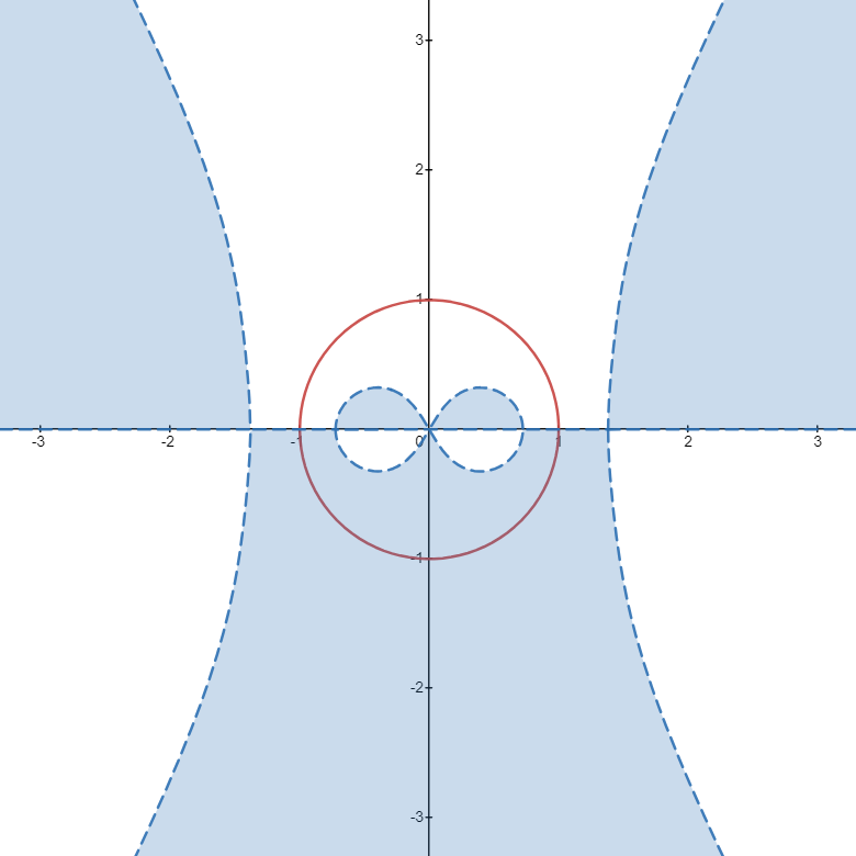
(a) $\xi<-6$

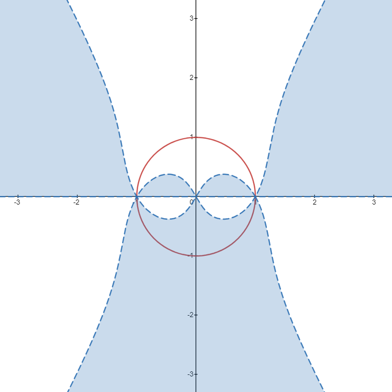
(b) $\xi=-6$

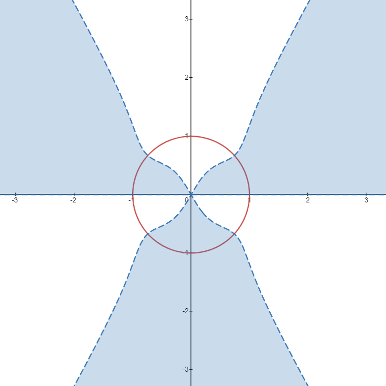
(c) $-6<\xi<-2$

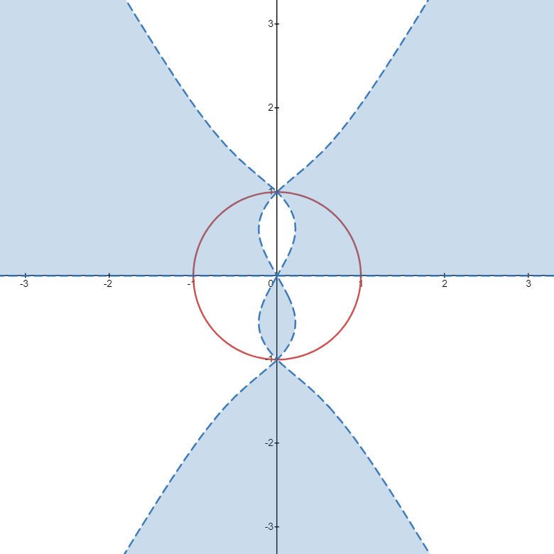
(d) $\xi=-2$

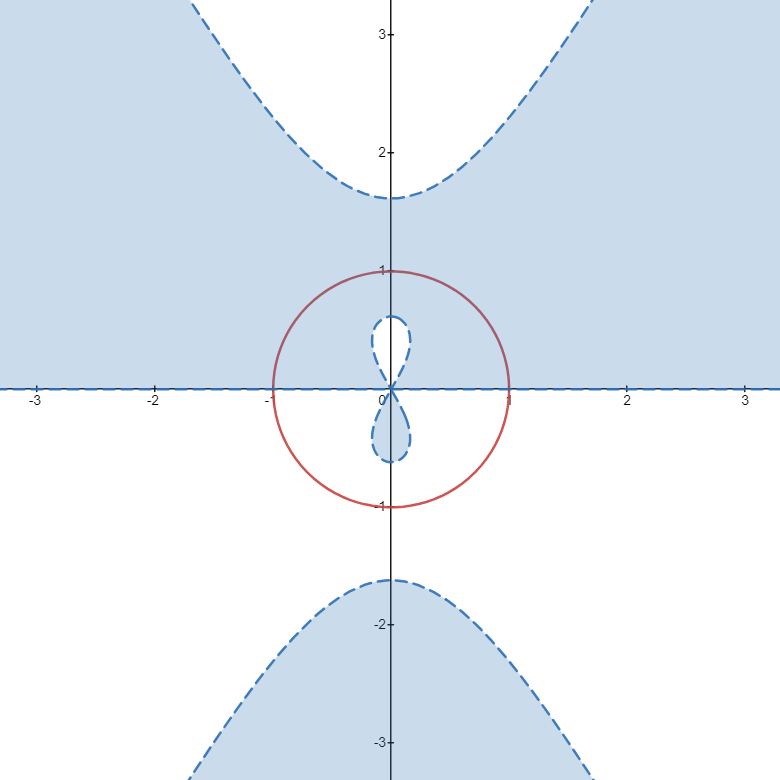
(e) $-2<\xi<6$

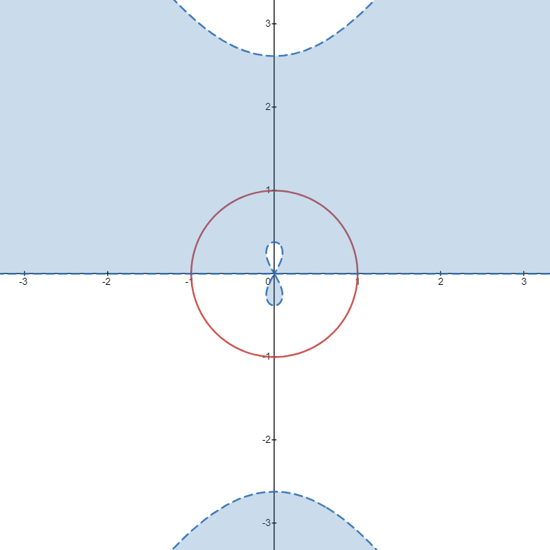
(f) $\xi\geq 6$

Figure 3: The distribution of saddle points and signature table of $\operatorname*{Re}(2i\theta(z))$, where $\operatorname*{Re}(2i\theta(z))<0$ is in blue regions and $\operatorname*{Re}(2i\theta(z))>0$ is in white regions. Figure (a): There are four saddle points on $\mathbb{R}$ for the solitonless region $\xi<-6$; Figure (c): There are four saddle points on the circle $|z|=1$ for the solitonic region $-6<\xi\leq-2$; Figure (e) and (f): There are four saddle points on $i\mathbb{R}$ for the solitonless region $\xi>-2$; Figures (b) and (d) are two critical cases.

The saddle points (or stationary phase points) satisfy the following equation

$$\theta^{\prime}(z)=\frac{(1+z^{2})(3z^{4}+\xi z^{2}+3)}{2z^{4}}=0,$$ (3.15)

which has the solutions

$$z^{2}=-1\ \ \text{or}\ \ z^{2}=\eta_{+}\ \ \text{or}\ \ z^{2}=\eta_{-},$$ (3.16)

where

$$\eta_{\pm}:=\frac{-\xi\pm\sqrt{\xi^{2}-36}}{6},\ \ |\xi|>6;\ \ \eta_{\pm}:=\frac{-\xi\pm i\sqrt{36-\xi^{2}}}{6},\ \ |\xi|<6.$$

Therefore, we have two fixed saddle points $\pm i$ and other four saddle points that vary with the value of $\xi$, distributed as follows.

If $\xi<-6$, then $\eta_{\pm}>0$ and four saddle points appear on the real axis

$$z_{1}=\sqrt{\eta_{+}},\ z_{2}=\sqrt{\eta_{-}},\ z_{3}=-\sqrt{\eta_{-}},\ z_{4}=-\sqrt{\eta_{+}},$$ (3.17)

with $z_{4}<-1<z_{3}<0<z_{2}<1<z_{1}$ and $z_{1}z_{2}=z_{3}z_{4}=1$. See Figure 3(a).

If $\xi>6$, then $\eta_{\pm}<0$ and four saddle points appear on the imaginary axis

$$z_{1}=i\sqrt{-\eta_{-}},\ z_{2}=i\sqrt{-\eta_{+}},\ z_{3}=-i\sqrt{-\eta_{+}},\ z_{4}=-i\sqrt{-\eta_{-}}$$ (3.18)

with $z_{4}<-i<z_{3}<0<z_{2}<i<z_{1}$ and $z_{1}z_{2}=z_{3}z_{4}=-1$. See Figure 3(f).

If $-6<\xi<6$, then $|\eta_{\pm}|=1$ and four saddle points appear on the unit circle $|z|=1$

$$z_{1}=e^{i\arg\eta_{+}/2},\ \ z_{2}=-e^{i\arg\eta_{+}/2},\ \ z_{3}=e^{i\arg\eta_{-}/2},\ \ z_{4}=-e^{i\arg\eta_{-}/2}.$$

See Figure 3(c) and 3(e).

Denote the critical line $\mathcal{L}:{\rm Re}(2i\theta(z))=0$ and the unit circle $\mathcal{C}:|z|=1$. By considering the cross points between $\mathcal{L}$ and $\mathcal{C}$, (3.14) simplifies to

$$2(u^{2}-v^{2})+\xi+4=0.$$ (3.19)

From this equation, we find that the cross points are $z=\pm 1$ on the real axis when $\xi=-6$ and $z=\pm i$ on the imaginary axis when $\xi=-2$, respectively. Based on the interaction between $\mathcal{L}$ and $\mathcal{C}$, we can classify the asymptotic regions as follows.

• Solitonless region: For the case $\xi<-6$ or $\xi>-2$, there is no interaction between $\mathcal{L}$ and $\mathcal{C}$. Moreover, $\mathcal{L}$ remains far way from $\mathcal{C}$, as depicted in Figure 3(a) and 3(e). This case corresponds to two distinct solitonless regions, which have been discussed in [33].

• Solitonic region: For the case $\xi=-2$, the merge points $z=\pm i$ do not appear on the contour $\mathbb{R}$, and in fact are just special poles when $\nu_{n}=-\bar{\nu}_{n}$. Therefore, for the case $-6<\xi\leq-2$, $\mathcal{L}$ interacts with $\mathcal{C}$, as shown in Figure 3(c) and 3(d). This is a solitonic region, in which the soliton resolution and the stability of $N$-solitons were investigated in [34].

• Transition region: For the case $\xi=-6$, the critical points are $z=\pm 1$ which are the merge points coming from four saddle points $z_{j},j=1,2,3,4$, as illustrated in Figure 3(b). Moreover, for the generic case, $|r(\pm 1)|=1$, it turns out that the norm $(1-|r(\pm 1)|^{2})^{-1}$ blows up as $z\to\pm 1$. This indicates the emergence of a new phenomenon in the transition region $\xi\approx-6$, which will be the focus of our investigation in the present paper.

3.3 A regular RH problem

We make two successive transformations to the basic RH problem 3.1 to obtain a regular RH problem without poles and singularities.

Step 1: Removing poles. Since the poles $\eta_{n}$ and $\overline{\eta}_{n}\in\mathcal{Z}$ are finite, distributed on the unit circle, and far way from the jump contour $\mathbb{R}$ and critical line $\mathcal{L}$, they decay exponentially when we convert their residues to jumps on small circles. This allows us to modify the basic RH problem 3.1 by removing these poles firstly.

To open the contour $\mathbb{R}$ by the second matrix decomposition in (3.12), we define the following scalar function

$$\delta(z)={\rm exp}\left(-i\int_{\mathbb{R}}\frac{\nu(\zeta)}{\zeta-z}\,\mathrm{d}\zeta\right),$$ (3.20)

where $\nu(\zeta)=-\frac{1}{2\pi}\log(1-|r(\zeta)|^{2})$, then it can be shown that

Proposition 3.1 ([34]).

The function $\delta(z)$ defined by (3.20) possesses the following properties:

• $\delta(z)$ is analytical in $\mathbb{C}\setminus\mathbb{R}$.

• $\delta(z)=\overline{\delta^{-1}(\bar{z})}=\overline{\delta(-\bar{z})}=\delta(z^{-1})^{-1}$.

• $\delta_{-}(z)=\delta_{+}(z)\left(1-|r(z)|^{2}\right),\ z\in\mathbb{R}$.

• The asymptotic behavior at infinity is

  $$\delta(\infty):=\lim_{z\rightarrow\infty}\delta(z)=1.$$ (3.21)

• $\frac{a(z)}{\delta(z)}$ is holomorphic and its absolute value is bounded in $\mathbb{C}^{+}$. Moreover, $\frac{a(z)}{\delta(z)}$ extends as a continuous function and its absolute value equals to $1$ for $z\in\mathbb{R}$.

Define

$$\rho<\frac{1}{2}{\rm min}\{\operatorname*{min}\limits_{\eta_{n},\eta_{j}\in\mathcal{Z}}|\eta_{n}-\eta_{j}|,\operatorname*{min}\limits_{\eta_{n}\in\mathcal{Z}}|\operatorname*{Im}\eta_{n}|,\operatorname*{min}\limits_{\eta_{n}\in\mathcal{Z},z\in\mathcal{L}}|\eta_{n}-z|\}.$$ (3.22)

For $\eta_{n}\in\mathcal{Z}$, we make small circles $C_{n},\,\bar{C}_{n}$ centered at $\eta_{n}$ and $\bar{\eta}_{n}$ with the radius $\rho$, and the corresponding disks $D_{n},\,\bar{D}_{n}$ lie inside the domain with respectively, $\operatorname*{Re}(2i\theta(z))>0$ for $\operatorname*{Im}z>0$ and $\operatorname*{Re}(2i\theta(z))<0$ for $\operatorname*{Im}z<0$. The circles are oriented counterclockwise in $\mathbb{C}^{+}$ and clockwise in $\mathbb{C}^{-}$. See Figure 4.

In order to interpolate the poles trading them for jumps on $C_{n}$ and $\bar{C}_{n}$, we construct the interpolation function

$$G(z)=\begin{cases}\left(\begin{array}[]{cc}1&0\\ -\displaystyle{\frac{c_{n}e^{-2it\theta(\eta_{n})}}{z-\eta_{n}}}&1\end{array}\right),\;z\in D_{n},\\ \left(\begin{array}[]{cc}1&-\displaystyle{\frac{\bar{c}_{n}e^{2it\theta(\bar{\eta}_{n})}}{z-\bar{\eta}_{n}}}\\ 0&1\end{array}\right),\;z\in\bar{D}_{n},\\ I,\;\;\;\text{elsewhere},\end{cases}$$ (3.23)

where $\eta_{n}\in\mathcal{Z}$.

Define

$$\Sigma^{(1)}=\mathbb{R}\cup\left(\bigcup_{n=1}^{2N}\left(C_{n}\cup\bar{C}_{n}\right)\right),$$

where the direction on $\mathbb{R}$ goes from left to right, as shown in Figure 4. For convenience, let

$$\Gamma=(-\infty,z_{4})\cup(z_{3},0)\cup(0,z_{2})\cup(z_{1},\infty).$$

Figure 4: The jump contour $\Sigma^{(1)}$ for $M^{(1)}(z)$. In the blue regions, $\operatorname*{Re}(2i\theta(z))<0$, while in the white regions, $\operatorname*{Re}(2i\theta(z))>0$.

Denoting the factorization of jump matrix by

$$\left(\begin{array}[]{cc}1&0\\ \frac{r(z)\delta_{-}(z)^{2}}{1-|r(z)|^{2}}e^{-2it\theta(z)}&1\end{array}\right)\left(\begin{array}[]{cc}1&-\frac{\overline{r(z)}\delta_{+}(z)^{-2}}{1-|r(z)|^{2}}e^{2it\theta(z)}\\ 0&1\end{array}\right):=B_{-}^{-1}B_{+},$$ (3.28)

and making the transformation

$$M^{(1)}(z)=M(z)G(z)\delta(z)^{\sigma_{3}},$$ (3.29)

$M^{(1)}(z)$ satisfies the symmetries of (3.11) and RH problem as follows.

RH problem 3.2.

Find $M^{(1)}(z)=M^{(1)}(z;x,t)$ with properties

• $M^{(1)}(z)$ is analytical in $\mathbb{C}\setminus\Sigma^{(1)}$.

• Jump condition:

  $$M^{(1)}_{+}(z)=M^{(1)}_{-}(z)V^{(1)}(z),$$

  where

  $$V^{(1)}(z)=\left\{\begin{array}[]{ll}B_{-}^{-1}B_{+},&z\in\Gamma,\\[8.0pt] \delta_{-}(z)^{-\sigma_{3}}V(z)\delta_{+}(z)^{\sigma_{3}},&z\in\mathbb{R}\setminus\Gamma,\\[6.0pt] \left(\begin{array}[]{cc}1&0\\ -\displaystyle{\frac{c_{n}e^{-2it\theta(\eta_{n})}\delta^{2}(z)}{z-\eta_{n}}}&1\end{array}\right),&z\in C_{n},\,n=1,\cdots,2N,\\[12.0pt] \left(\begin{array}[]{cc}1&\displaystyle{\frac{\bar{c}_{n}e^{2it\theta(\bar{\eta}_{n})}\delta^{-2}(z)}{z-\bar{\eta}_{n}}}\\ 0&1\end{array}\right),&z\in\bar{C}_{n},\,n=1,\cdots,2N.\end{array}\right.$$

• Asymptotic behaviors:

  $$M^{(1)}(z)=I+\mathcal{O}(z^{-1}),\quad z\to\infty,$$

  $$zM^{(1)}(z)=\sigma_{2}+\mathcal{O}(z),\quad z\to 0.$$

Since the jump matrices on the circles $C_{n}$ and $\bar{C}_{n}$ exponentially decay to the identity matrix as $t\to\infty$, RH problem 3.2 can be approximated by the following RH problem.

RH problem 3.3.

Find $M^{(2)}(z)=M^{(2)}(z;x,t)$ with properties

• $M^{(2)}(z)$ is analytical in $\mathbb{C}\setminus\mathbb{R}$.

• Jump condition:

  $$M^{(2)}_{+}(z)=M^{(2)}_{-}(z)V^{(2)}(z),$$

  where

  $$V^{(2)}(z)=\left\{\begin{array}[]{ll}B_{-}^{-1}B_{+},\;z\in\Gamma,\\[6.0pt] \delta_{-}(z)^{-\sigma_{3}}V(z)\delta_{+}(z)^{\sigma_{3}},\;z\in\mathbb{R}\setminus\Gamma.\end{array}\right.$$ (3.30)

• Asymptotic behaviors:

  $$M^{(2)}(z)=I+\mathcal{O}(z^{-1}),\quad z\to\infty,$$

  $$zM^{(2)}(z)=\sigma_{2}+\mathcal{O}(z),\quad z\to 0.$$

It can be shown that the solution $M^{(1)}(z)$ is asymptotically equivalent to $M^{(2)}(z)$.

Proposition 3.2.

$$M^{(1)}(z)=M^{(2)}(z)\left(I+\mathcal{O}(e^{-ct})\right),$$ (3.31)

where $c$ is a constant. From the symmetry of (3.30), one can check directly that

$$M^{(2)}(z)=\sigma_{1}M^{(2)*}(z)\sigma_{1}=\overline{M^{(2)}(-\bar{z})}=\mp z^{-1}M^{(2)}(z^{-1})\sigma_{2}.$$

Step 2: Removing singularities. In order to remove the singularity $z=0$, we make a transformation

$$M^{(2)}(z)=\left(I+\frac{\sigma_{2}}{z}M^{(3)}(0)^{-1}\right)M^{(3)}(z),$$ (3.32)

then $M^{(2)}(z)$ satisfies the RH problem 3.3 if $M^{(3)}(z)$ satisfies the following RH problem.

RH problem 3.4.

Find $M^{(3)}(z)=M^{(3)}(z;x,t)$ with properties

• $M^{(3)}(z)$ is analytical in $\mathbb{C}\setminus\mathbb{R}$.

• Jump condition: $M^{(3)}_{+}(z)=M^{(3)}_{-}(z)V^{(2)}(z),$ where $V^{(2)}(z)$ is given by (3.30).

• Asymptotic behavior: $M^{(3)}(z)=I+\mathcal{O}(z^{-1}),\quad z\to\infty.$

Moreover, it is straightforward to check that $M^{(3)}(z)$ satisfies the symmetries

$$M^{(3)}(z)=\sigma_{1}M^{(3)*}(z)\sigma_{1}=\overline{M^{(3)}(-\bar{z})}=\sigma_{1}M^{(3)}(0)^{-1}M^{(3)}(z^{-1})\sigma_{1}.$$

Proof.

The proof is similar to the proof in [23, RH problem 3.3]. ∎

4 Asymptotics analysis in the transition region

In this section, we consider the asymptotics in the region $-C<(\xi+6)t^{2/3}<0$ with $C>0$ which corresponds to Figure 3(a). In this case, the two saddle points $z_{1}$ and $z_{2}$ defined by (3.17) are real and close to $z=1$ at least the speed of $t^{-1/3}$ as $t\to+\infty$. Meanwhile, the other two saddle points $z_{3}$ and $z_{4}$ defined by (3.17) are close to $z=-1$.

4.1 A hybrid $\bar{\partial}$-RH problem

Fix a sufficiently small angle $\phi=\phi(\xi)$ such that $\phi$ satisfies the following conditions:

• $0<\phi<\arccos\frac{1}{\sqrt{5}-1}<\frac{\pi}{4}$.

• each $\Omega_{j},\,j=0^{\pm},1,2,3,4$ does not intersect with $\mathcal{L}$;

• each $\Omega_{j},\,j=0^{\pm},1,2,3,4$ does not intersect any small disks $D_{n},\,\bar{D}_{n},\,n=1,\cdots,2N$,

where $\Omega_{j},\,j=0^{\pm},1,2,3,4$ are defined by

$$\Omega_{0^{+}}:=\{z\in\mathbb{C}:0\leq\arg z\leq\phi,\,|\operatorname*{Re}z|\leq\frac{z_{2}}{2}\},\ \Omega_{0^{-}}:=\{z\in\mathbb{C}:-\bar{z}\in\Omega_{0^{+}}\},$$

$$\Omega_{1}:=\{z\in\mathbb{C}:0\leq\arg(z-z_{1})\leq\phi\},\quad\Omega_{4}:=\{z\in\mathbb{C}:-\bar{z}\in\Omega_{1}\},$$

$$\Omega_{2}:=\{z\in\mathbb{C}:\pi-\phi\leq\arg(z-z_{2})\leq\pi,\,|\operatorname*{Re}(z-z_{2})|\leq\frac{z_{2}}{2}\},\,\Omega_{3}:=\{z\in\mathbb{C}:-\bar{z}\in\Omega_{2}\}.$$

Then, ${\Omega}^{*}_{j}$ are the conjugate regions of $\Omega_{j}$. Moreover, to open the jump contour $\Gamma$ by the $\bar{\partial}$ extension, we define $\Sigma_{j},\,j=0^{\pm},1,2,3,4$ as the boundaries of $\Omega_{j}$ and denote

$$l\in\left(0,\frac{z_{2}}{2}\tan\phi\right),\quad\Sigma^{\prime}_{n}=(-1)^{n+1}\frac{z_{2}}{2}+e^{i\frac{\pi}{2}}l,\quad n=1,2.$$

${\Sigma}^{*}_{j},\,j=0^{\pm},1,2,3,4$ and ${\Sigma}^{\prime*}_{n},\,n=1,2$ denote the conjugate contours above. See Figure 5. Denote

$$\Sigma=\bigcup_{j=0^{\pm},1,2,3,4}(\Sigma_{j}\cup\Sigma_{j}^{*}),\ \ \Sigma^{\prime}=\bigcup_{n=1,2}(\Sigma^{\prime}_{n}\cup\Sigma^{\prime*}_{n}),\ \ \Omega=\bigcup_{j=0^{\pm},1,2,3,4}(\Omega_{j}\cup{\Omega}^{*}_{j}).$$

Figure 5: Open the jump contour $\Gamma$. The region where $\operatorname*{Re}\left(2i\theta(z)\right)<0$ is in blue.

To determine the decaying properties of the oscillating factors $e^{\pm 2it\theta(z)}$, we especially estimate the $\operatorname*{Re}(2i\theta(z))$ in different regions.

Proposition 4.1.

Let $-C<\left(\frac{x}{t}+6\right)t^{2/3}<0$. Denote $z=|z|e^{i\phi_{0}}$. Then the following estimates hold.

• $($corresponding to $z=0$$)$

  $$\operatorname*{Re}(2i\theta(z))\leq-c_{0}|\sin\phi_{0}||\operatorname*{Im}z|,\quad z\in\Omega_{0^{+}}\cup\Omega_{0^{-}},$$ (4.1)

  $$\operatorname*{Re}(2i\theta(z))\geq c_{0}|\sin\phi_{0}||\operatorname*{Im}z|,\quad z\in{\Omega}^{*}_{0^{+}}\cup{\Omega}^{*}_{0^{-}},$$ (4.2)

  where $c_{0}=c_{0}(\phi_{0},\xi)$ is a constant.

• $($corresponding to $z=z_{j},j=1,4$$)$

  $$\operatorname*{Re}(2i\theta(z))\leq\begin{cases}-c_{j}|\operatorname*{Re}z-z_{j}|^{2}|\operatorname*{Im}z|,\quad z\in\Omega_{j}\cap\{|z|\leq 2\},\\ -c_{j}|\operatorname*{Im}z|,\quad z\in\Omega_{j}\cap\{|z|>2\},\end{cases}$$ (4.3)

  $$\operatorname*{Re}(2i\theta(z))\geq\begin{cases}c_{j}|\operatorname*{Re}z-z_{j}|^{2}|\operatorname*{Im}z|,\quad z\in{\Omega}^{*}_{j}\cap\{|z|\leq 2\},\\ c_{j}|\operatorname*{Im}z|,\quad z\in{\Omega}^{*}_{j}\cap\{|z|>2\},\end{cases}$$ (4.4)

  where $c_{j}=c_{j}(z_{j},\phi_{0},\xi)$ is a constant.

• $($corresponding to $z=z_{j},j=2,3$$)$

  $$\operatorname*{Re}(2i\theta(z))\leq-c_{j}|\operatorname*{Re}z-z_{j}|^{2}|\operatorname*{Im}z|,\quad z\in\Omega_{j},$$ (4.5)

  $$\operatorname*{Re}(2i\theta(z))\geq c_{j}|\operatorname*{Re}z-z_{j}|^{2}|\operatorname*{Im}z|,\quad z\in{\Omega}^{*}_{j},$$ (4.6)

  where $c_{j}=c_{j}(z_{j},\phi_{0},\xi)$ is a constant.

Proof.

For the case corresponding to $z=0$, we take $\Omega_{0^{+}}$ as an example to prove the estimate (4.1). Others can be proven in a similar way.

For $z\in\Omega_{0^{+}}$, denote the ray $z=|z|e^{i\phi_{0}}=u+iv$ where $0<\phi_{0}<\phi$ and $u>v>0$, and the function $F(l)=l+l^{-1}$. Then, (3.14) becomes

$$\operatorname*{Re}\left(2i\theta(z)\right)=-F(|z|)\sin\phi_{0}\left((1+2\cos 2\phi_{0})F(|z|)^{2}-6\cos 2\phi_{0}+\xi\right).$$ (4.7)

Considering $(1+2\cos 2\phi_{0})F(|z|)^{2}-6\cos 2\phi_{0}+\xi=0$, we have

$$F(|z|)^{2}=3-\frac{3+\xi}{2\cos 2\phi_{0}+1}:=\alpha>4.$$

By $F(l)=\sqrt{\alpha}$, we have $l^{2}-\sqrt{\alpha}l+1=0$. Solving the above equation, we find two roots

$$l_{1}=\frac{\sqrt{\alpha}-\sqrt{\alpha-4}}{2}<l_{2}=\frac{\sqrt{\alpha}+\sqrt{\alpha-4}}{2}.$$

Since $|z|\leq\frac{z_{2}\sec\phi_{0}}{2}<l_{1}$,

$$(1+2\cos 2\phi_{0})F(|z|)^{2} -6\cos 2\phi_{0}+\xi\geq$$

$$(1+2\cos 2\phi_{0})F\left(\frac{z_{2}\sec\phi_{0}}{2}\right)^{2}-6\cos 2\phi_{0}+\xi>0.$$

Thus there exists a constant $c_{0}=c_{0}(\phi_{0})$ such that

$$\operatorname*{Re}\left(2i\theta(z)\right)\leq c_{0}F(|z|)\sin\phi_{0}.$$

For the cases corresponding to $z_{j},j=1,4$, we take $\Omega_{1}$ as an example and others can be easily inferred. Let $z=z_{1}+u+iv$. Then (3.14) can be rewritten as

$$\operatorname*{Re}\left(2i\theta(z)\right)=-vF(u,v),$$ (4.8)

where

$$F(u,v)=(\xi+3)\left(1+|z|^{-2}\right)+\left(3(z_{1}+u)^{2}-v^{2}\right)\left(1+|z|^{-6}\right).$$ (4.9)

For $z\in\Omega_{1}$ and $|z|\leq 2$, from (3.17), we have

$$\xi=-3z_{1}^{-2}(1+z_{1}^{4}).$$ (4.10)

Substituting (4.10) into (4.9) yields

$$F(u,v)=z_{1}^{-2}|z|^{-6}G(u,v),$$ (4.11)

where

$$G(u,v)=3\left(z_{1}^{2}-1-z_{1}^{4}\right)\left(|z|^{6}+|z|^{4}\right)+\left(3z_{1}^{2}(z_{1}+u)^{2}-z_{1}^{2}v^{2}\right)\left(|z|^{6}+1\right).$$ (4.12)

After simplification, we obtain

$$G(u,v)\geq 16z_{1}^{2}u^{2},$$

then

$$F(u,v)\geq 16u^{2}|z|^{-6}\ \text{and}\ \operatorname*{Re}\left(2i\theta(z)\right)\leq-16|z|^{-6}u^{2}v.$$

Since $|z|\leq 2$,

$$\operatorname*{Re}\left(2i\theta(z)\right)\leq-\frac{1}{4}u^{2}v.$$

Moreover, the proof for the cases corresponding to $z_{j},j=2,3$ can be given similarly.

Next we consider the estimate for $z\in\Omega_{1}$ and $|z|>2$. In the transition region, $\xi\to-6^{-}$, (4.9) reduces to

$$F(u,v)=\left(1+|z|^{-6}\right)\left(-3f(|z|)+3(z_{1}+u)^{2}-v^{2}\right),$$ (4.13)

where

$$f(x)=\frac{x^{6}+x^{4}}{x^{6}+1}.$$ (4.14)

Since $f(x)$ has a maximum value $f_{max}=\frac{4}{3}$,

$$F(u,v)\geq-4+3(z_{1}+u)^{2}-v^{2}.$$

Let $z=|z|e^{i\phi_{0}}$ with $0<\phi_{0}<\phi$. Notice that $v=(z_{1}+u)\tan w$ where $0<w<\phi_{0}$, we obtain

$$F(u,v)\geq-4+2(z_{1}+u)^{2}\geq-4+8\cos^{2}\phi_{0}\geq-4+\frac{8}{(\sqrt{5}-1)^{2}}.$$

Until now we finish the proof for the estimate (4.3) in $\Omega_{1}$. ∎

Next we open the contour $\Gamma$ via continuous extensions of the jump matrix $V^{(2)}(z)$ by defining appropriate functions.

Proposition 4.2.

Let $q_{0}\in\tanh(x)+H^{4,4}(\mathbb{R})$. Then it is possible to define functions $R_{j}:\overline{\Omega}_{j}\to\mathbb{C},\ j=0^{\pm},1,2,3,4$, continuous on $\overline{\Omega}_{j}$, with continuous first partials on $\Omega_{j}$, and boundary values

$$R_{j}(z)=\begin{cases}\frac{\overline{r(z)}\delta_{+}(z)^{-2}}{1-|r(z)|^{2}},\quad z\in\Gamma,\\ \gamma(z_{j}),\quad z\in\Sigma_{j},\end{cases}$$

where

$$\gamma(z)=\begin{cases}\frac{\overline{S_{21}(z)}}{S_{11}(z)}\left(\frac{a(z)}{\delta_{+}(z)}\right)^{2},\quad\text{\rm for the generic case},\\[5.01874pt] \frac{\overline{r(z)}\delta_{+}(z)^{-2}}{1-|r(z)|^{2}},\quad\text{\rm for the non-generic case},\end{cases}$$ (4.15)

with

$$S_{21}(z)={\rm det}(\Phi_{-,1}(z),\Phi_{+,1}(z)),$$ (4.16)

$$S_{11}(z)={\rm det}(\Phi_{+,1}(z),\Phi_{-,2}(z)),$$ (4.17)

and $\gamma(0)=0$, such that for $j=1,2$; a fixed constant $c=c(q_{0})$; and a fixed cutoff function $\varphi\in C^{\infty}_{0}(\mathbb{R},[0,1])$ with small support near $1$; we have

$$|\bar{\partial}R_{j}(z)|\leq c\left(|r^{\prime}\left(|z|\right)|+|z-z_{j}|^{-1/2}+\varphi(|z|)\right),\;z\in\Omega_{j},$$ (4.18)

$$|\bar{\partial}R_{j}(z)|\leq c|z-1|,\;z\in\Omega_{j}\ \text{in a small fixed neighborhood of}\ 1;$$ (4.19)

for $j=3,4$, we have (4.18) with $|z|$ replaced by $-|z|$ in the argument of $r^{\prime}$ and $\varphi$, as well as (4.19); for $j=0^{\pm}$, we have

$$|\bar{\partial}R_{0^{\pm}}(z)|\leq c\left(|r^{\prime}\left(\pm|z|\right)|+|z|^{-1/2}\right),\;z\in\Omega_{0}^{\pm}.$$ (4.20)

The similar estimate holds for $|\bar{\partial}R^{*}_{j}(z)|$.

Setting $R:\Omega\to\mathbb{C}$ by $R(z)|_{z\in\Omega_{j}}=R_{j}(z)$ and $R(z)|_{z\in{\Omega}^{*}_{j}}=R^{*}_{j}(z)$, the extension can preserve the symmetry $R(z)=-\overline{R(\bar{z}^{-1})}$.

Proof.

The proof is similar to those in the soliton region [33] or solitonless region [34]. We omit it here. ∎

Define

$$R^{(3)}(z)=\begin{cases}\left(\begin{array}[]{cc}1&R_{j}(z)e^{2it\theta(z)}\\ 0&1\end{array}\right),\quad z\in\Omega_{j},\;j=0^{\pm},1,2,3,4,\\ \left(\begin{array}[]{cc}1&0\\ {R}^{*}_{j}(z)e^{-2it\theta(z)}&1\end{array}\right),\quad z\in{\Omega}^{*}_{j},\;j=0^{\pm},1,2,3,4,\\ I,\quad{\rm elsewhere},\end{cases}$$ (4.21)

and a contour

$$\Sigma^{(4)}=\Sigma\cup\Sigma^{\prime}\cup[z_{4},z_{3}]\cup[z_{2},z_{1}].$$

See Figure 6.

Then the new matrix-valued function

$$M^{(4)}(z)=M^{(3)}(z)R^{(3)}(z)$$ (4.22)

satisfies the following hybrid $\bar{\partial}$-RH problem.

$\bar{\partial}$-RH problem 4.1.

Find $M^{(4)}(z)=M^{(4)}(z;x,t)$ with properties

• $M^{(4)}(z)$ is continuous in $\mathbb{C}\setminus\Sigma^{(4)}$ and takes continuous boundary values $M^{(4)}_{+}(z)$ $($respectively $M^{(4)}_{-}(z))$ on $\Sigma^{(4)}$ from the left $($respectively right$)$.

• $M^{(4)}(z)$ satisfies the jump condition

  $$M^{(4)}_{+}(z)=M^{(4)}_{-}(z)V^{(4)}(z),\quad z\in\Sigma^{(4)},$$

where

$$V^{(4)}(z)=\begin{cases}\left(\begin{array}[]{cc}1&-\gamma(z_{j})e^{2it\theta(z)}\\ 0&1\end{array}\right),\ z\in\Sigma_{j},\ j=1,2,3,4,\vspace{2mm}\\ \left(\begin{array}[]{cc}1&0\\ \overline{\gamma(z_{j})}e^{-2it\theta(z)}&1\end{array}\right),\ z\in{\Sigma}^{*}_{j},\ j=1,2,3,4,\vspace{2mm}\\ \left(\begin{array}[]{cc}1&-\gamma(z_{2})e^{2it\theta(z)}\\ 0&1\end{array}\right),\ z\in\Sigma^{\prime}_{1},\vspace{2mm}\\ \left(\begin{array}[]{cc}1&0\\ \overline{\gamma(z_{2})}e^{-2it\theta(z)}&1\end{array}\right),\ z\in{\Sigma}^{*^{\prime}}_{1},\vspace{2mm}\\ \left(\begin{array}[]{cc}1&\gamma(z_{3})e^{2it\theta(z)}\\ 0&1\end{array}\right),\ z\in\Sigma^{\prime}_{2},\vspace{2mm}\\ \left(\begin{array}[]{cc}1&0\\ -\overline{\gamma(z_{3})}e^{-2it\theta(z)}&1\end{array}\right),\ z\in{\Sigma}^{*^{\prime}}_{2},\vspace{2mm}\\ \delta_{-}(z)^{-\sigma_{3}}V(z)\delta_{+}(z)^{\sigma_{3}},\quad z\in\mathbb{R}\setminus\Gamma.\end{cases}$$ (4.23)

• $M^{(4)}(z)=I+\mathcal{O}(z^{-1}),\quad z\to\infty.$

• For $z\in\mathbb{C}$, we have

  $$\bar{\partial}M^{(4)}(z)=M^{(4)}(z)\bar{\partial}R^{(3)}(z),$$

  where

  $$\bar{\partial}R^{(3)}(z)=\begin{cases}\left(\begin{array}[]{cc}0&\bar{\partial}R_{j}(z)e^{2it\theta(z)}\\ 0&0\end{array}\right),\quad z\in\Omega_{j},\;j=0^{\pm},1,2,3,4,\\ \left(\begin{array}[]{cc}0&0\\ \bar{\partial}{R}^{*}_{j}(z)e^{-2it\theta(z)}&0\end{array}\right),\quad z\in\Omega^{*}_{j},\ j=0^{\pm},1,2,3,4,\\ 0,\quad\text{elsewhere}.\end{cases}$$ (4.24)

Until now we have obtained the hybrid $\bar{\partial}$-RH problem 4.1 for $M^{(4)}(z)$ to analyze the long-time asymptotics of the original RH problem 3.1 for $M(z)$. Next, we will construct the solution $M^{(4)}(z)$ as follows:

• We first remove the $\bar{\partial}$ component of the solution $M^{(4)}(z)$ and demonstrate the existence of a solution of the resulting pure RH problem. Furthermore, we calculate its asymptotic expansion.

• Conjugating off the solution of the first step, a pure $\bar{\partial}$-problem can be obtained. Then, we establish the existence of a solution to this problem and bound its size.

Figure 6: The jump contour $\Sigma^{(4)}$ for $M^{(4)}(z)$ and $M^{rhp}(z)$.

4.2 Contribution from a pure RH problem

In this subsection, we first consider the pure RH problem. Dropping the $\bar{\partial}$ component of $M^{(4)}(z)$, $M^{rhp}(z)$ satisfies the following pure RH problem.

RH problem 4.1.

Find $M^{rhp}(z)=M^{rhp}(z;x,t)$ which satisfies

• $M^{rhp}(z)$ is analytical in $\mathbb{C}\setminus\Sigma^{(4)}$. See Figure 6.

• $M^{rhp}(z)$ satisfies the jump condition

  $$M^{rhp}_{+}(z)=M^{rhp}_{-}(z)V^{(4)}(z),$$

  where $V^{(4)}(z)$ is given by (4.23).

• $M^{rhp}(z)$ has the same asymptotics with $M^{(4)}(z)$.

According to the property of $V^{(4)}-I$, we now analyse the local model $M^{loc}(z)$ of $M^{rhp}(z)$ in the neighborhood of $z=\pm 1$.

4.2.1 Local paramatrix

Let $t$ be large enough so that $\sqrt{2C}(3t)^{-1/3+\epsilon}<\rho$ where $\epsilon$ is a constant with $0<\epsilon<\frac{1}{9}$ and $\rho$ has been defined in (3.22). For a fixed constant $\varepsilon\leq\sqrt{2C}$, define two open disks

$$\mathcal{U}_{r}=\{z\in\mathbb{C}:|z-1|<(3t)^{-1/3+\epsilon}\varepsilon\},\ \ \mathcal{U}_{l}=\{z\in\mathbb{C}:|z+1|<(3t)^{-1/3+\epsilon}\varepsilon\}.$$

Denote the local jump contour

$$\Sigma^{loc}:=\Sigma^{(4)}\cap\left(\mathcal{U}_{r}\cup\mathcal{U}_{l}\right),$$

as depicted in Figure 7. The local model $M^{loc}(z)$ satisfies the following RH problem.

Figure 7: The jump contour $\Sigma^{loc}$ for $M^{loc}(z)$.

RH problem 4.2.

Find $M^{loc}(z)=M^{loc}(z;x,t)$ which satisfies

• $M^{loc}(z)$ is analytical in $\mathbb{C}\setminus\Sigma^{loc}$.

• $M^{loc}(z)$ satisfies the jump condition

  $$M^{loc}_{+}(z)=M^{loc}_{-}(z)V^{loc}(z),$$

  where $V^{loc}(z):=V^{(4)}(z)|_{z\in\Sigma^{loc}}$.

• $M^{loc}(z)$ has the same asymptotics with $M^{rhp}(z)$.

Based on the theorem of Beals-Coifman, we know as $t\to\infty$, the solution $M^{loc}(z)$ is approximated by the sum of the separate local model in the neighborhood of $1$ and $-1$ respectively. On the contours $\Sigma_{j}:=\Sigma^{(4)}\cap\mathcal{U}_{j},\,j\in\{r,l\}$ (moreover, $\Sigma^{loc}=\Sigma_{r}\cup\Sigma_{l}$), we define the local models $M^{j}(z),\,j\in\{r,l\}$ respectively.

RH problem 4.3.

Find $M^{j}(z)=M^{j}(z;x,t)$ with properties

• $M^{j}(z)$ is analytical in $\mathbb{C}\setminus{\Sigma}_{j}$.

• $M^{j}(z)$ satisfies the jump condition

  $$M^{j}_{+}(z)=M^{j}_{-}(z){V}^{j}(z),\ z\in{\Sigma}_{j},$$

  where ${V}^{j}(z)=V^{(4)}(z)|_{z\in\Sigma_{j}},\,j\in\{r,l\}$.

• As $z\to\infty$ in $\mathbb{C}\setminus{\Sigma}_{j}$, $M^{j}(z)=I+\mathcal{O}(z^{-1})$.

In the region $-C<(\xi+6)t^{2/3}<0$ with $C>0$, we notice that $\xi\to-6^{-}$ as $t\to\infty$, further from (3.17), it is found that two saddle points $z_{1}$ and $z_{2}$ will merge to $z=1$, while $z_{3}$ and $z_{4}$ will merge to $z=-1$ as $\xi\to-6^{-}$.

The phase faction $t\theta(z)$ can be approximated with the help of scaled spectral variables:

• For $z$ close to $1$,

  $$t\theta(z)=4t(z-1)^{3}+(6t+x)(z-1)+A(z),$$ (4.25)

  where

  $$A(z)=\frac{1}{2}\left(3t(z-1)^{2}-7t(z-1)^{3}+\sum_{n=2}^{\infty}(-1)^{n+1}\left(x+\frac{n^{2}+3n+8}{2}t\right)(z-1)^{n}\right).$$ (4.26)

  Observing the characteristics of the above expansion, we introduce the following scaled spectral variables to match with the coefficients of the exponential terms in the Painlevé II RH model, as defined in A:

  Define $s$ be the space-time parameter and $\hat{k}$ be the scaled parameter

  $$s=\frac{1}{3}(\xi+6)(3t)^{2/3},\quad\hat{k}=(3t)^{1/3}(z-1),$$ (4.27)

  then it can be proven that $A(z)$ converges and $A(z)=\mathcal{O}(t^{-1/3}\hat{k}^{2})$. Therefore, (4.25) becomes

  $$t\theta(z)=\frac{4}{3}\hat{k}^{3}+s\hat{k}+\mathcal{O}(t^{-1/3}\hat{k}^{2}).$$ (4.28)

• For $z$ close to $-1$,

  $$t\theta(z)=4t(z+1)^{3}+(6t+x)(z+1)+A(z),$$ (4.29)

  where

  $$A(z)=\frac{1}{2}\left(-3t(z+1)^{2}-7t(z+1)^{3}+\sum_{n=2}^{\infty}\left(x+\frac{n^{2}+3n+8}{2}t\right)(z+1)^{n}\right).$$ (4.30)

  Similar to the case for $z\to 1$, the space-time parameter $s$ is defined as (4.27) and we define the scaled parameter $\check{k}$ as

  $$\check{k}=(3t)^{1/3}(z+1).$$ (4.31)

  Then $A(z)$ converges and $A(z)=\mathcal{O}(t^{-1/3}\check{k}^{2})$. Therefore, (4.29) becomes

  $$t\theta(z)=\frac{4}{3}\check{k}^{3}+s\check{k}+\mathcal{O}(t^{-1/3}\check{k}^{2}).$$ (4.32)

Remark 4.3.

For the case of the mKdV equation (1.1) with ZBCs, the phase function is

$$t\theta(z)=4tz^{3}+xz.$$ (4.33)

We carry out the following scaling:

$$z\to kt^{-1/3}$$

and (4.33) becomes

$$t\theta(kt^{-1/3})=4k^{3}+xkt^{-1/3}=3(\frac{4}{3}k^{3}+sk),$$

where $s=\frac{1}{3}\xi t^{-2/3}$ with $\xi=x/t$. This indicates under this conditions, the local model can precisely match the exponential term coefficients of the Painlevé II RH model. However, in the case of NBCs (1.1)-(1.2), the phase function can only approximate the exponential term coefficients of the Painlevé II RH model with an error of $\mathcal{O}(t^{-1/3}k^{2})$.

Next we define two open disks associated with the scaled parameters $\hat{k}$ and $\check{k}$

$$\widehat{\mathcal{U}}_{r}=\{\hat{k}\in\mathbb{C}:|\hat{k}|<(3t)^{\epsilon}\varepsilon\},\ \ \widecheck{\mathcal{U}}_{l}=\{\check{k}\in\mathbb{C}:|\check{k}|<(3t)^{\epsilon}\varepsilon\},$$

whose boundaries are oriented counterclockwise. Then the transformation given by (4.27) define a map $z\mapsto\hat{k}$, which maps $\mathcal{U}_{r}$ onto $\widehat{\mathcal{U}}_{r}$ in the $\hat{k}$-plane, while the transformation given by (4.31) maps $\mathcal{U}_{l}$ onto $\widecheck{\mathcal{U}}_{l}$ in the $\check{k}$-plane.

Figure 8: The jump contour $\widehat{\Sigma}_{r}$ for $M^{r}(\hat{k})$ on $\widehat{\mathcal{U}}_{r}$.

First, we construct the local parametrix $M^{r}(z)$. Define the contour $\widehat{\Sigma}_{r}$ in the $\hat{k}$-plane

$$\widehat{\Sigma}_{r}:=\bigcup_{j=1,2}\left(\widehat{\Sigma}_{j}\cup\widehat{\Sigma}^{*}_{j}\right)\cup(\hat{k}_{2},\hat{k}_{1})$$

which corresponds to $\Sigma_{r}$ after scaling $z$ to the scaled parameter $\hat{k}$. The corresponding regions in the $\hat{k}$-plane can be seen in Figure 8. Correspondingly, the saddle points $z_{1}$, $z_{2}$ in the $z$-plane are rescaled to $\hat{k}_{1}$, $\hat{k}_{2}$ respectively in the $\hat{k}$-plane with $\hat{k}_{j}=(3t)^{1/3}(z_{j}-1),j=1,2$. Moreover, (4.27) also reveals that

$$z=(3t)^{-1/3}\hat{k}+1.$$

Therefore, the jump matrix $V^{r}(z)$ transforms to the following $V^{r}(\hat{k})$ in the $\hat{k}$-plane

$$V^{r}(\hat{k})=\begin{cases}e^{it\theta\left((3t)^{-1/3}\hat{k}+1\right)\widehat{\sigma}_{3}}\left(\begin{array}[]{cc}1&-\gamma(z_{j})\\ 0&1\end{array}\right),\ \hat{k}\in\widehat{\Sigma}_{j},\ j=1,2,\\ e^{it\theta\left((3t)^{-1/3}\hat{k}+1\right)\widehat{\sigma}_{3}}\left(\begin{array}[]{cc}1&0\\ \overline{\gamma(z_{j})}&1\end{array}\right),\ \hat{k}\in\widehat{\Sigma}^{*}_{j},\ j=1,2,\\ \delta_{-}\left((3t)^{-1/3}\hat{k}+1\right)^{-\sigma_{3}}V\left((3t)^{-1/3}\hat{k}+1\right)\delta_{+}\left((3t)^{-1/3}\hat{k}+1\right)^{\sigma_{3}},\ \hat{k}\in[\hat{k}_{2},\hat{k}_{1}].\end{cases}$$

For the generic case, $z_{j}\to 1$ and $r(z_{j})\to-i$ for $j=1,2$ as $t\to\infty$, which causes the appearance of the singularity of $\frac{r(z_{j})}{1-|r(z_{j})|^{2}}$. However, this singularity can be balanced by the factor $T(z)^{-2}$. Define a cutoff function $\chi(z)\in C_{0}^{\infty}(\mathbb{R},[0,1])$ satisfying

$$\chi(z)=1,\ z\in\mathbb{R}\cap\mathcal{U}_{r},$$ (4.34)

and a new reflection coefficient $\tilde{r}(z)$ satisfying

$$\tilde{r}(z)=(1-\chi(z))\frac{\overline{r(z)}}{1-|r(z)|^{2}}\delta_{+}(z)^{-2}+\chi(z)f(z)h(z)^{2},$$ (4.35)

where

$$f(z):=\frac{\overline{S_{21}(z)}}{S_{11}(z)},\ \ \ h(z):=\frac{a(z)}{\delta_{+}(z)},$$

and $S_{21}(z)$ and $S_{11}(z)$ are defined by (4.16) and (4.17) respectively, while for the non-generic case,

$$\tilde{r}(z)=\frac{\overline{r(z)}}{1-|r(z)|^{2}}\delta_{+}(z)^{-2}.$$ (4.36)

Moreover, we have $\tilde{r}(z_{j})=\gamma(z_{j})$ as $z_{j}\to 1,\ j=1,2$.

Next we will show that in the $\widehat{\mathcal{U}}_{r}$, RH problem for $M^{r}(\hat{k})$ can be explicitly approximated by the following model RH problem for $\widehat{M}^{r}(\hat{k})$, and then prove the solution $\widehat{M}^{r}(\hat{k})$ is associated to Painlevé II transcendents.

RH problem 4.4.

Find $\widehat{M}^{r}(\hat{k})=\widehat{M}^{r}(\hat{k};x,t)$ with properties

• $\widehat{M}^{r}(\hat{k})$ is analytical in $\mathbb{C}\setminus\widehat{\Sigma}_{r}$.

• $\widehat{M}^{r}(k)$ satisfies the jump condition

  $$\widehat{M}^{r}_{+}(\hat{k})=\widehat{M}^{r}_{-}(\hat{k})\widehat{V}^{r}(\hat{k}),\ \hat{k}\in\widehat{\Sigma}_{r},$$

where

$$\widehat{V}^{r}(\hat{k})=\begin{cases}e^{i\left(\frac{4}{3}\hat{k}^{3}+s\hat{k}\right)\widehat{\sigma}_{3}}\left(\begin{array}[]{cc}1&-\tilde{r}(1)\\ 0&1\end{array}\right):=b_{+}^{-1},\ \hat{k}\in\widehat{\Sigma}_{j},\ j=1,2,\\ e^{i\left(\frac{4}{3}\hat{k}^{3}+s\hat{k}\right)\widehat{\sigma}_{3}}\left(\begin{array}[]{cc}1&0\\ \overline{\tilde{r}(1)}&1\end{array}\right):=b_{-},\ \hat{k}\in\widehat{\Sigma}^{*}_{j},\ j=1,2,\\ b_{-}b_{+}^{-1},\ \hat{k}\in[\hat{k}_{2},\hat{k}_{1}].\end{cases}$$

• $\widehat{M}^{r}(\hat{k})\to I,\ \hat{k}\to\infty$.

Define $N(\hat{k}):=M^{r}(\hat{k})(\widehat{M}^{r}(\hat{k}))^{-1}$ which satisfies the following RH problem.

RH problem 4.5.

Find $N(\hat{k})=N(\hat{k};x,t)$ such that

• $N(\hat{k})$ is analytical in $\mathbb{C}\setminus\widehat{\Sigma}_{r}$.

• $N(\hat{k})$ satisfies the following jump condition

  $$N_{+}(\hat{k})=N_{-}(\hat{k})V^{N}(\hat{k}),$$

  where

  $$V^{N}(\hat{k})=\widehat{M}_{-}^{r}(\hat{k})V^{r}(\hat{k})\widehat{V}^{r}(\hat{k})^{-1}\widehat{M}_{-}^{r}(\hat{k})^{-1}.$$

Proposition 4.4.

As $t\to\infty$, $N(\hat{k})$ exists and satisfies

$$N(\hat{k})=I+\mathcal{O}(t^{-\frac{1}{3}+2\epsilon}),$$ (4.37)

where $\epsilon$ is a constant with $0<\epsilon<\frac{1}{9}$.

Proof.

Suppose that $\widehat{M}^{r}(\hat{k})$ is bounded, which we will show in (4.49) and (4.51), we only need to estimate the error between $V^{r}(\hat{k})$ and $\widehat{V}^{r}(\hat{k})$. For $\hat{k}\in\left(\hat{k}_{2},\hat{k}_{1}\right)$, $\left|e^{2it\theta(z)}\right|=\left|e^{i(\frac{8}{3}\hat{k}^{3}+2s\hat{k})}\right|=1$. Direct calculations show that

$$\left|\tilde{r}(z)e^{2it\theta\left(z\right)}-\tilde{r}(1)e^{i(\frac{8}{3}\hat{k}^{3}+2s\hat{k})}\right|$$

$$\leq\left|\tilde{r}(z)-\tilde{r}(1)\right|+\left|\tilde{r}(1)\right|\left|e^{2it\theta\left(z\right)}-e^{i(\frac{8}{3}\hat{k}^{3}+2s\hat{k})}\right|$$

$$\leq\left|h(z)\right|^{2}\left|f(z)-f(1)\right|+\left|f(1)\right|\left|h^{2}(z)-h^{2}(1)\right|$$

$$+\left|\tilde{r}(1)\right|\left|e^{2it\theta\left(z\right)}-e^{i(\frac{8}{3}\hat{k}^{3}+2s\hat{k})}\right|$$ (4.38)

Following the idea of Proposition 3.2 in [33], with the Hölder inequality, we have

$$\left|f(z)-f(1)\right|\leq\|r\|_{H^{1}(\mathbb{R})}|z-1|^{\frac{1}{2}}t^{-\frac{1}{6}}\lesssim t^{-\frac{1}{3}+\frac{\epsilon}{2}},$$ (4.39)

$$\left|e^{i\mathcal{O}(t^{-\frac{1}{3}}\hat{k}^{2})}-1\right|\leq e^{|\mathcal{O}(t^{-\frac{1}{3}}\hat{k}^{2})|}-1\lesssim t^{-\frac{1}{3}+2\epsilon}.$$ (4.40)

From (2.28) and (3.20), it is straightforward to check that

$$h(z)=\prod_{n=1}^{2N}\frac{z-\eta_{n}}{z-\bar{\eta}_{n}},$$ (4.41)

then,

$$|h(z)-h(1)|\leq\left|\prod_{n=1}^{2N}\frac{1-\eta_{n}}{1-\bar{\eta}_{n}}\right|\left|\prod_{n=1}^{2N}\frac{z-\eta_{n}}{z-\bar{\eta}_{n}}\frac{1-\bar{\eta}_{n}}{1-\eta_{n}}-1\right|\lesssim t^{-\frac{2}{3}+2\epsilon}.$$ (4.42)

Substituting (4.39), (4.40), and (4.42) into (4.38), we obtain

$$\Big{|}\tilde{r}(z)e^{2it\theta\left(z\right)}-\tilde{r}(1)e^{i\left(\frac{8}{3}\hat{k}^{3}+2s\hat{k}\right)}\Big{|}\lesssim t^{-\frac{1}{3}+2\epsilon}.$$ (4.43)

For $\hat{k}\in\widehat{\Sigma}_{1}$, denote $\hat{k}=\hat{k}_{1}+\hat{u}+i\hat{v}$ and $z=z_{1}+u+iv$. To prove that $\operatorname*{Re}i\left(\frac{8}{3}\hat{k}^{3}+2s\hat{k}\right)\leq-\frac{16}{3}\hat{u}^{2}\hat{v}$ holds, we only need to prove the following inequality holds

$$\operatorname*{Re}i\left(8t(z-1)^{3}+2(x+6t)(z-1)\right)\leq-16u^{2}v.$$ (4.44)

From (4.10), it is easy to infer that

$$\operatorname*{Re}i\left(8t(z-1)^{3}+2(x+6t)(z-1)\right)\leq-16tu^{2}v-2tvw(z_{1}),$$ (4.45)

where

$$w(z_{1})=12(z_{1}-1)^{2}+24(z_{1}-1)u-\frac{3\left(z_{1}^{4}+1\right)}{z_{1}^{2}}+6.$$ (4.46)

Since $w^{\prime}(z_{1})\geq 0$ on the interval $[1,+\infty)$, $w(z_{1})\geq w(1)=0$ and then

$$\operatorname*{Re}i\left(8t(z-1)^{3}+2(x+6t)(z-1)\right)\leq-16tu^{2}v.$$ (4.47)

Therefore, $\left|e^{i\left(\frac{8}{3}\hat{k}^{3}+2s\hat{k}\right)}\right|$ is bounded. Similarly to the case on the real axis, we can obtain

$$\Big{|}\tilde{r}(z_{j})e^{2it\theta\left(z\right)}-\tilde{r}(1)e^{i\left(\frac{8}{3}\hat{k}^{3}+2s\hat{k}\right)}\Big{|}\lesssim t^{-\frac{1}{3}+2\epsilon},\ \hat{k}\in\widehat{\Sigma}_{1}.$$ (4.48)

The estimate on other jump contours can be given in a similar way. (4.43) and (4.48) implies that $\|V^{N}-I\|_{L^{1}\cap L^{2}\cap L^{\infty}}\lesssim t^{-\frac{1}{3}+2\epsilon}$ uniformly. Therefore, the existence and uniqueness of $N(\hat{k})$ can be proven by the theorem of the small-norm RH problem [39], which also yields (4.37).

∎

Therefore, the solution $\widehat{M}^{r}(\hat{k})$ is crucial to our analysis. Next we show it can be transformed into a standard Painlevé II equation via an appropriately equivalent deformation. For this purpose, we add four new auxiliary paths $L_{j},j=1,2,3,4$ passing through the point $\hat{k}=0$ at the angle $\pi/3$ with real axis, which together with the original paths $\widehat{\Sigma}_{r}$ divide the complex plane into 10 regions $\widetilde{\Omega}_{j},j=1,\cdots,6$ and $\widehat{\Omega}_{j}\cup\widehat{\Omega}^{*}_{j},j=1,2$. See Figure 9.

We further define

$$P(\hat{k})=\left\{\begin{matrix}b_{+},\ \ &\hat{k}\in\widetilde{\Omega}_{1}\cup\widetilde{\Omega}_{3},\cr b_{-},\ \ &\hat{k}\in\widetilde{\Omega}_{4}\cup\widetilde{\Omega}_{6},\cr I,\ \ &\text{elsewhere},\end{matrix}\right.$$

and make a transformation

$$\widetilde{M}^{r}(\hat{k})=\widehat{M}^{r}(\hat{k})P(\hat{k}),$$ (4.49)

then we obtain the following RH problem.

RH problem 4.6.

Find $\widetilde{M}^{r}(\hat{k})=\widetilde{M}^{r}(\hat{k};s)$ with properties

• $\widetilde{M}^{r}(\hat{k})$ is analytical in $\mathbb{C}\setminus\widetilde{\Sigma}^{P}$, where $\widetilde{\Sigma}^{P}=\cup_{j=1}^{4}L_{j}.$ See Figure 9.

• $\widetilde{M}^{r}(\hat{k})$ satisfies the jump condition

  $$\widetilde{M}^{r}_{+}(\hat{k})=\widetilde{M}^{r}_{-}(\hat{k})\widetilde{V}^{P}(\hat{k}),\ \ \hat{k}\in\widetilde{\Sigma}^{P},$$

  where

  $$\widetilde{V}^{P}(\hat{k})=\begin{cases}b_{+}^{-1},\quad\hat{k}\in L_{1}\cup L_{2},\\ b_{-},\quad\hat{k}\in L_{3}\cup L_{4}.\end{cases}$$ (4.50)

• $\widetilde{M}^{r}(\hat{k})\to I,\ \hat{k}\to\infty$.

Figure 9: In the plot(a), add four new dashed auxiliary lines on the jump contour for $\widehat{M}^{r}(\hat{k})$, which then can be deformed into the Painlevé II RH model $M^{P}(\hat{k})$ with the jump contour of four lines (see the plot (b)).

Let

$$\varphi_{0}=\arg\tilde{r}(1)=\arg\bar{r}(1)-\frac{1}{\pi}\int_{\mathbb{R}}\frac{\log(1-|r(\zeta)|^{2})}{\zeta-1}\,\mathrm{d}\zeta.$$

Then

$$\tilde{r}(1)=|\tilde{r}(1)|e^{i\varphi_{0}},\quad\text{with}\quad|\tilde{r}(1)|=|r(1)|.$$

Following the idea [40], we find the solution $\widetilde{M}^{r}(\hat{k})$ can be expressed by

$$\widetilde{M}^{r}(\hat{k})=\sigma_{1}e^{-i\left(\frac{\pi}{4}+\frac{\varphi_{0}}{2}\right)\widehat{\sigma}_{3}}M^{P}(\hat{k})\sigma_{1},$$ (4.51)

where $M^{P}(\hat{k})$ satisfies a standard Painlevé II RH problem given in A with $p=|\tilde{r}(1)|$. By Proposition 4.4, we have

$$M^{r}_{1}(s)=\widetilde{M}^{r}_{1}(s)+\mathcal{O}(t^{-\frac{1}{3}+2\epsilon})=\sigma_{1}e^{-i\left(\frac{\pi}{4}+\frac{\varphi_{0}}{2}\right)\widehat{\sigma}_{3}}M^{P}_{1}(s)\sigma_{1}+\mathcal{O}(t^{-\frac{1}{3}+2\epsilon}),$$ (4.52)

where the subscript “$1$” represents the coefficient of the Taylor expansion of the term $\hat{k}^{-1}$ as $\hat{k}\to\infty$, and $M^{P}_{1}(s)$ is given by (A.5) with $p=|\tilde{r}(1)|$. Finally, the long-time solution of $M^{r}(z)$ can be described by the following equation.

$$M^{r}(z)=I+\frac{M^{r}_{1}(s)}{(3t)^{1/3}(z-1)}+\mathcal{O}(t^{-\frac{2}{3}+2\epsilon}).$$ (4.53)

A similar process gives the solution $M^{l}(z)$, which has the asymptotics

$$M^{l}(z)=I+\frac{M^{l}_{1}(s)}{(3t)^{1/3}(z+1)}+\mathcal{O}(t^{-\frac{2}{3}+2\epsilon}),$$ (4.54)

where

$$M^{l}_{1}(s)=-\sigma_{1}M^{r}_{1}(s)\sigma_{1}.$$ (4.55)

Now we construct the solution $M^{rhp}(z)$ of the form

$$M^{rhp}(z)=\begin{cases}E(z),\ z\in\mathbb{C}\setminus\left(\mathcal{U}_{r}\cup\mathcal{U}_{l}\right),\\ E(z)M^{r}(z),\ z\in\mathcal{U}_{r},\\ E(z)M^{l}(z),\ z\in\mathcal{U}_{l}.\end{cases}$$ (4.56)

Since the solution $M^{j}(z),\,j\in\{r,l\}$ have been obtained, we can construct the solution $M^{rhp}(z)$ if we find the error function $E(z)$.

4.2.2 A small-norm RH problem

We consider the error function $E(z)$ defined by (4.56), which admits the following RH problem.

Figure 10: The jump contour $\Sigma^{E}$ for $E(z)$.

RH problem 4.7.

Find $E(z)$ with the properties

• $E(z)$ is analytical in $\mathbb{C}\setminus\Sigma^{E}$, where $\Sigma^{E}=\left(\partial\mathcal{U}_{r}\cup\partial\mathcal{U}_{l}\right)\cup\left(\Sigma^{(4)}\setminus\left(\mathcal{U}_{r}\cup\mathcal{U}_{l}\right)\right)$. See Figure 10.

• $E(z)$ satisfies the jump condition

  $$E_{+}(z)=E_{-}(z)V^{E}(z),\quad z\in\Sigma^{E},$$

  where the jump matrix is given by

  $$V^{E}(z)=\begin{cases}V^{(4)}(z),\quad z\in\Sigma^{(4)}\setminus\left(\mathcal{U}_{r}\cup\mathcal{U}_{l}\right),\\ M^{r}(z),\quad z\in\partial\mathcal{U}_{r},\\ M^{l}(z),\quad z\in\partial\mathcal{U}_{l}.\end{cases}$$ (4.57)

• $E(z)=I+\mathcal{O}(z^{-1}),\quad z\to\infty.$

To obtain the existence of the solution $E(z)$, we estimate the jump matrix $V^{E}(z)-I$ .

Proposition 4.5.

For $2\leq p\leq\infty$ and $0<\epsilon<\frac{1}{9}$, there exists a constant $c$ such that

$$||V^{E}(z)-I||_{L^{p}(\Sigma^{E})}=\begin{cases}\mathcal{O}(e^{-ct}),\quad z\in\Sigma^{E}\setminus\left(\mathcal{U}_{r}\cup\mathcal{U}_{l}\right),\\ \mathcal{O}(t^{-\frac{1}{3p}+\frac{1-p}{p}\epsilon}),\quad z\in\partial\mathcal{U}_{r}\cup\partial\mathcal{U}_{l}.\end{cases}$$ (4.58)

Proof.

First, we consider the estimate when $p=\infty$. For $z\in\Sigma^{E}\setminus\left(\mathcal{U}_{r}\cup\mathcal{U}_{l}\right)$, by (4.57) and Proposition 4.1,

$$|V^{E}(z)-I|=|V^{(4)}(z)-I|\lesssim e^{-ct},$$ (4.59)

where $c=c(\phi,\xi)$. For $z\in\partial\mathcal{U}_{r}$, by (4.57),

$$|V^{E}(z)-I|=|M^{r}(z)-I|\lesssim t^{-\epsilon}.$$ (4.60)

So does the estimate on $\partial\mathcal{U}_{l}$. Other cases when $2\leq p<\infty$ can be proven similarly. ∎

This proposition establishes RH problem 4.7 as a small-norm RH problem, for which there is a well-known existence and uniqueness theorem [39]. Define the Cauchy integral operator $C_{w^{E}}:L^{2}(\Sigma^{E})\to L^{2}(\Sigma^{E})$ by

$$C_{w^{E}}f=C_{-}\left(f\left(V^{E}(z)-I\right)\right),$$

where $w^{E}=V^{E}(z)-I$ and $C_{-}$ is the Cauchy projection operator on $\Sigma^{E}$. By (4.58), a simple calculation shows that

$$||C_{w^{E}}||_{L^{2}(\Sigma^{E})}\lesssim||C_{-}||_{L^{2}(\Sigma^{E})}||V^{E}(z)-I||_{L^{\infty}(\Sigma^{E})}\lesssim t^{-\epsilon}.$$

According to the theorem of Beals-Coifman [41], the solution of RH problem 4.7 can be expressed in terms of

$$E(z)=I+\frac{1}{2\pi i}\int_{\Sigma^{E}}\frac{\mu_{E}(\zeta)\left(V^{E}(\zeta)-I\right)}{\zeta-z}\,\mathrm{d}\zeta,$$

where $\mu_{E}\in L^{2}\left(\Sigma^{E}\right)$ satisfies $\left(I-C_{w^{E}}\right)\mu_{E}=I$. Furthermore, from (4.58), we have the estimates

$$||V^{E}(z)-I||_{L^{2}}\lesssim t^{-\frac{1}{6}-\frac{\epsilon}{2}},\quad||\mu_{E}-I||_{L^{2}}\lesssim t^{-\frac{1}{6}-\frac{\epsilon}{2}},$$ (4.61)

which imply that RH problem 4.7 exists an unique solution.

To recover the potential $q(x,t)$ of (3.10), we need the properties of $E(z)$ at $z=0$ and $z=\infty$. We make the expansion of $E(z)$ at $z=\infty$

$$E(z)=I+z^{-1}E_{1}+\mathcal{O}\left(z^{-2}\right),$$ (4.62)

where

$$E_{1}=-\frac{1}{2\pi i}\int_{\Sigma^{E}}\mu_{E}(\zeta)\left(V^{E}(\zeta)-I\right)\,\mathrm{d}\zeta.$$

Proposition 4.6.

$E_{1}$ and $E(0)$ can be estimated as follows:

$$E_{1}=(3t)^{-\frac{1}{3}}\begin{pmatrix}i\int_{s}^{\infty}u(\zeta)^{2}\mathrm{d}\zeta&iu(s)\cos\varphi_{0}\\ -iu(s)\cos\varphi_{0}&-i\int_{s}^{\infty}u(\zeta)^{2}\mathrm{d}\zeta\end{pmatrix}+\mathcal{O}\left(t^{-\frac{1}{3}-\epsilon}\right),$$ (4.63)

$$E(0)=I+(3t)^{-\frac{1}{3}}\begin{pmatrix}0&u(s)\sin\varphi_{0}\\ u(s)\sin\varphi_{0}&0\end{pmatrix}+\mathcal{O}\left(t^{-\frac{1}{3}-\epsilon}\right).$$ (4.64)

Proof.

By (4.57) and (4.61), we obtain that

$$E_{1} =-\frac{1}{2\pi i}\oint_{\partial\mathcal{U}_{r}}\left(V^{E}(\zeta)-I\right)\mathrm{d}\zeta-\frac{1}{2\pi i}\oint_{\partial\mathcal{U}_{l}}\left(V^{E}(\zeta)-I\right)\mathrm{d}\zeta+\mathcal{O}\left(t^{-\frac{1}{3}-\epsilon}\right)$$

$$=(3t)^{-\frac{1}{3}}\left(M^{r}_{1}(s)+M^{l}_{1}(s)\right)+\mathcal{O}\left(t^{-\frac{1}{3}-\epsilon}\right),$$

which gives (4.63) by the estimates (4.52) and (4.55).

In a similar way, we have

$$E(0) =I+\frac{1}{2\pi i}\oint_{\partial\mathcal{U}_{r}}\frac{V^{E}(\zeta)-I}{\zeta}\mathrm{d}\zeta+\frac{1}{2\pi i}\oint_{\partial\mathcal{U}_{l}}\frac{V^{E}(\zeta)-I}{\zeta}\mathrm{d}\zeta+\mathcal{O}\left(t^{-\frac{1}{3}-\epsilon}\right)$$

$$=I-(3t)^{-\frac{1}{3}}\left(M^{r}_{1}(s)-M^{l}_{1}(s)\right)+\mathcal{O}\left(t^{-\frac{1}{3}-\epsilon}\right),$$

which yields (4.64) by the estimates (4.52) and (4.55). ∎

4.3 Contribution from a pure $\bar{\partial}$-problem

Here we consider the long-time asymptotic behavior for the pure $\bar{\partial}$-problem $M^{(5)}(z)$. Define the function

$$M^{(5)}(z)=M^{(4)}(z)\left(M^{rhp}(z)\right)^{-1},$$ (4.65)

which satisfies the following $\bar{\partial}$-problem.

$\bar{\partial}$-problem 4.1.

Find $M^{(5)}(z):=M^{(5)}(z;x,t)$ which satisfies

• $M^{(5)}(z)$ is continuous in $\mathbb{C}$ and analytic in $\mathbb{C}\setminus\overline{\Omega}$.

• $M^{(5)}(z)=I+\mathcal{O}(z^{-1}),\ z\to\infty$.

• For $z\in\mathbb{C}$, $M^{(5)}(z)$ satisfies the $\bar{\partial}$-equation

  $$\bar{\partial}M^{(5)}(z)=M^{(5)}(z)W^{(5)}(z),$$

  where

  $$W^{(5)}(z):=M^{rhp}(z)\bar{\partial}R^{(3)}(z)\left(M^{rhp}(z)\right)^{-1},$$ (4.66)

  and $\bar{\partial}R^{(3)}(z)$ has been given in (4.24).

The solution of $\bar{\partial}$-RH problem 4.1 can be given by

$$M^{(5)}(z)=I-\frac{1}{\pi}\iint_{\mathbb{C}}\frac{M^{(5)}(\zeta)W^{(5)}(\zeta)}{\zeta-z}\,\mathrm{d}\zeta\wedge\mathrm{d}\bar{\zeta},$$ (4.67)

which can be written as an operator equation

$$(I-S)M^{(5)}(z)=I,$$ (4.68)

where $S$ is the solid Cauchy operator

$$Sf(z)=-\frac{1}{\pi}\iint_{\mathbb{C}}\frac{f(\zeta)W^{(5)}(\zeta)}{\zeta-z}\,\mathrm{d}\zeta\wedge\mathrm{d}\bar{\zeta}.$$ (4.69)

Proposition 4.7.

The operator $S$ defined by (4.69) satisfies the estimate

$$\parallel S\parallel_{L^{\infty}(\mathbb{C})\to L^{\infty}(\mathbb{C})}\lesssim t^{-1/6},$$ (4.70)

which implies the existence of $(I-S)^{-1}$ for large $t$.

Proof.

We estimate the operator $S$ on $\Omega_{1}$ and other cases are similar. In fact, by (4.18), (4.21), (4.66), and (4.69), there exists a constant $c$ such that

$$\|Sf\|_{L^{\infty}\to L^{\infty}}\leq c(I_{1}+I_{2}+I_{3}+I_{4}),$$

where

$$I_{1}=\iint_{\Omega_{1}\cap\{|z|\leq 2\}}F(\zeta,z)\mathrm{d}\zeta\wedge\mathrm{d}\bar{\zeta},\ \ I_{2}=\iint_{\Omega_{1}\cap\{|z|>2\}}F(\zeta,z)\mathrm{d}\zeta\wedge\mathrm{d}\bar{\zeta},$$

$$I_{3}=\iint_{\Omega_{1}\cap\{|z|\leq 2\}}G(\zeta,z)\mathrm{d}\zeta\wedge\mathrm{d}\bar{\zeta},\ \ \ I_{4}=\iint_{\Omega_{1}\cap\{|z|>2\}}G(\zeta,z)\mathrm{d}\zeta\wedge\mathrm{d}\bar{\zeta}.$$

with

$$F(\zeta,z)=\frac{1}{|\zeta-z|}\left|r^{\prime}(|\zeta|)\right|e^{\operatorname*{Re}(2it\theta(z))},\ G(\zeta,z)=\frac{1}{|\zeta-z|}\left|\zeta-z_{1}\right|^{-1/2}e^{\operatorname*{Re}(2it\theta(z))}.$$

Let $y=\operatorname*{Im}z$ and $\zeta=z_{1}+u+iv=|\zeta|e^{iw}$. Using Proposition 4.1 and the Cauchy-Schwartz’s inequality, we have

$$I_{1} =\int_{0}^{2\sin w}\int_{v}^{2\cos w-z_{1}}F(\zeta,z)\mathrm{d}u\mathrm{d}v$$

$$\lesssim\int_{0}^{2\sin w}||r^{\prime}||_{L^{2}(\mathbb{R})}|v-y|^{-1/2}e^{-c_{1}tv^{3}}\mathrm{d}v\lesssim t^{-1/6},$$

$$I_{2} =\int_{2\sin w}^{\infty}\int_{2\cos w-z_{1}}^{\infty}F(\zeta,z)\mathrm{d}u\mathrm{d}v$$

$$\lesssim\int_{2\sin w}^{\infty}||r^{\prime}||_{L^{2}(\mathbb{R})}|v-y|^{-1/2}e^{-c_{1}tv}\mathrm{d}v\lesssim t^{-1/2}.$$

In a similar way, using Proposition 4.1 and the Hölder’s inequality with $p>2$ and $1/p+1/q=1$, we obtain

$$I_{3} \lesssim\int_{0}^{2\sin w}v^{1/p-1/2}|v-y|^{1/q-1}e^{-c_{1}tv^{3}}\mathrm{d}v\lesssim t^{-1/6},$$

$$I_{4} \lesssim\int_{2\sin w}^{\infty}v^{1/p-1/2}|v-y|^{1/q-1}e^{-c_{1}tv}\mathrm{d}v\lesssim t^{-1/2}.$$

∎

Proposition 4.7 implies that the operator equation (4.68) exists an unique solution, which can be expanded in the form

$$M^{(5)}(z)=I+z^{-1}M^{(5)}_{1}(x,t)+\mathcal{O}(z^{-2}),\quad z\to\infty,$$ (4.71)

where

$$M^{(5)}_{1}(x,t)=\frac{1}{\pi}\iint_{\mathbb{C}}M^{(5)}(\zeta)W^{(5)}(\zeta)\,\mathrm{d}\zeta\wedge\mathrm{d}\bar{\zeta}.$$ (4.72)

Take $z=0$ in (4.67), then

$$M^{(5)}(0)=I-\frac{1}{\pi}\iint_{\mathbb{C}}\frac{M^{(5)}(\zeta)W^{(5)}(\zeta)}{\zeta}\mathrm{d}\zeta\wedge\mathrm{d}\bar{\zeta}.$$ (4.73)

Proposition 4.8.

We have the following estimates

$$|M^{(5)}_{1}(x,t)|\lesssim t^{-1/2},\ \ \ |M^{(5)}(0)-I|\lesssim t^{-1/2}.$$ (4.74)

Proof.

Similarly to the proof of Proposition 4.7, we take $z\in\Omega_{1}$ as an example and divide the integration (4.72) on $\Omega_{1}$ into four parts. Firstly, we consider the estimate of $M^{(5)}_{1}(x,t)$. By (4.65) and the boundedness of $M^{(4)}(z)$ and $M^{rhp}(z)$ on $\Omega_{1}$, we have

$$|M^{(5)}_{1}(x,t)|\lesssim I_{1}+I_{2}+I_{3}+I_{4},$$ (4.75)

where

$$I_{1}=\iint_{\Omega_{1}\cap\{|z|\leq 2\}}F(\zeta,z)\mathrm{d}\zeta\wedge\mathrm{d}\bar{\zeta},\ \ I_{2}=\iint_{\Omega_{1}\cap\{|z|>2\}}F(\zeta,z)\mathrm{d}\zeta\wedge\mathrm{d}\bar{\zeta},$$

$$I_{3}=\iint_{\Omega_{1}\cap\{|z|\leq 2\}}G(\zeta,z)\mathrm{d}\zeta\wedge\mathrm{d}\bar{\zeta},\ \ \ I_{4}=\iint_{\Omega_{1}\cap\{|z|>2\}}G(\zeta,z)\mathrm{d}\zeta\wedge\mathrm{d}\bar{\zeta}.$$

with

$$F(\zeta,z)=\left|r^{\prime}(|\zeta|)\right|e^{\operatorname*{Re}(2it\theta(z))},\ G(\zeta,z)=\left|\zeta-z_{1}\right|^{-1/2}e^{\operatorname*{Re}(2it\theta(z))}.$$

Let $\zeta=z_{1}+u+iv=|\zeta|e^{iw}$. By Cauchy-Schwartz’s inequality and Proposition 4.1, we have

$$I_{1} \lesssim\int_{0}^{2\sin w}\int_{v}^{2\cos w-z_{1}}\left|r^{\prime}(|\zeta|)\right|e^{-c_{1}tv^{3}}\mathrm{d}u\mathrm{d}v\lesssim t^{-1/2},$$

$$I_{2} \lesssim\int_{2\sin w}^{\infty}\int_{2\cos w-z_{1}}^{\infty}\left|r^{\prime}(|\zeta|)\right|e^{-c_{1}tv}\mathrm{d}u\mathrm{d}v\lesssim t^{-3/2}.$$

By Hölder’s inequality with $p>2$ and $1/p+1/q=1$ and Proposition 4.1, we have

$$I_{3} \lesssim\int_{0}^{2\sin w}\int_{0}^{2\cos w-z_{1}}\left|u+iv\right|^{-1/2}e^{-c_{1}tv^{3}}\mathrm{d}u\mathrm{d}v\lesssim t^{-1/2},$$

$$I_{4} \lesssim\int_{2\sin w}^{\infty}\int_{2\cos w-z_{1}}^{\infty}\left|u+iv\right|^{-1/2}e^{-c_{1}tv}\mathrm{d}u\mathrm{d}v\lesssim t^{-3/2}.$$

Then we estimate $M^{(5)}(0)-I$. Notice that if $z\in\Omega_{1}$, then $|z|^{-1}\leq|z_{1}|^{-1}$. By (4.73) and (4.75), we get $|M^{(5)}(0)-I|\lesssim t^{-1/2}$.

∎

To recover the potential from the reconstruction formula (3.10), we need the estimate for $M^{(3)}(0)$.

Proposition 4.9.

As $t\to+\infty$, $M^{(3)}(0)$ satisfies the estimate

$$M^{(3)}(0)=E(0)+\mathcal{O}(t^{-1/2}),$$ (4.76)

where $E(0)$ is given by (4.64).

Proof.

Reviewing the series of transformations (4.22), (4.56), and (4.65) , for large $z$ and satisfying $R^{(3)}(z)=I$, the solution of $M^{(3)}(z)$ is given by

$$M^{(3)}(z)=M^{(5)}(z)E(z).$$

By (4.71) and (4.74), we further obtain

$$M^{(3)}(z)=E(z)+\mathcal{O}(t^{-1/2}),$$

which yields (4.76) by taking $z=0$. ∎

4.4 Painlevé asymptotics

In this subsection, we state and prove main results in this paper as follows.

Theorem 4.10.

For initial data $q_{0}\in\tanh(x)+H^{4,4}(\mathbb{R})$, let $r(z)$ and $\{\nu_{j}\}_{j=0}^{N-1}$ be, respectively, the associated reflection coefficient and the discrete spectrum. We also define the corresponding modified reflection coefficient $\tilde{r}(z)$ given by (4.35)-(4.36). Then the long-time asymptotics of the solution to the Cauchy problem (1.1)-(1.2) for the defocusing mKdV equation in the transition region $\left|\frac{x}{t}+6\right|t^{2/3}<C$ with $C>0$ is given by the following formula:

$$q(x,t)=-1+(3t)^{-\frac{1}{3}}u(s)\cos\varphi_{0}+\mathcal{O}\left(t^{-\frac{1}{3}-\epsilon}\right),$$ (4.77)

where $\epsilon$ is a constant with $0<\epsilon<\frac{1}{9}$,

$$s=\frac{1}{3}(3t)^{\frac{2}{3}}\left(\frac{x}{t}+6\right),\ \varphi_{0}=\arg\tilde{r}(1),$$

and $u(s)$ is a solution of the Painlevé II equation

$$u_{ss}(s)=2u^{3}(s)+su(s),$$ (4.78)

which admits the asymptotics

$$u(s)\sim-|r(1)|\mathrm{Ai}(s)\sim-|r(1)|\frac{1}{2\sqrt{\pi}}s^{-\frac{1}{4}}e^{-\frac{2}{3}s^{3/2}},\ s\to+\infty,$$ (4.79)

where $\mathrm{Ai}(s)$ is the classical Airy function.

Proof.

Inverting the sequence of transformations (3.29), (3.32), (4.22), (4.56), (4.65), and especially taking $z\to\infty$ vertically such that $R^{(3)}(z)=G(z)=I$, then the solution of RH problem 3.1 is given by

$$M(z)=\left(I+\frac{\sigma_{2}}{z}M^{(3)}(0)^{-1}\right)M^{(5)}(z)E(z)\delta(z)^{-\sigma_{3}}+\mathcal{O}(e^{-ct}).$$

Further substituting asymptotic expansions (3.21), (4.62), and (4.71) into the above formula, the reconstruction formula (3.10) yields

$$q(x,t)=i\left(\sigma_{2}M^{(3)}(0)^{-1}+E_{1}\right)+\mathcal{O}\left(t^{-\frac{1}{3}-\epsilon}\right).$$ (4.80)

Utilizing (4.63) and (4.76), we arrive at the result stated as (4.77) in Theorem 4.10. ∎

Appendix A Painlevé II RH problem

The Painlevé II equation is

$$u_{ss}(s)=2u^{3}(s)+su(s),\quad s\in\mathbb{R},$$ (A.1)

which can be solved by means of RH problem as follows.

Figure 11: The jump contour $\Sigma^{P}$ and the corresponding jump matrix for $M^{P}(k)$.

Denote $\Sigma^{P}=\bigcup_{j=1}^{6}\left\{\Sigma_{j}^{P}=e^{i\left(\frac{\pi}{6}+(j-1)\frac{\pi}{3}\right)}\mathbb{R}_{+}\right\}$, see Figure 11. The Painlevé II RH problem satisfies the following properties:

RH problem A.1.

Find $M^{P}(k)=M^{P}(k;s,t)$ with properties

• Analyticity: $M^{P}(k)$ is analytical in $\mathbb{C}\setminus\Sigma^{P}$.

• Jump condition:

  $$M^{P}_{+}(k)=M^{P}_{-}(k)e^{-i(\frac{4}{3}k^{3}+sk)\widehat{\sigma}_{3}}V^{P}(k),$$

  where $V^{P}(k)$ is shown in Figure 11. The parameters $p$, $q$, and $r$ in $V^{P}(k)$ satisfy the relation

  $$r=p+q+pqr.$$ (A.2)

• Asymptotic behaviors:

  $$M^{P}(k)=I+\mathcal{O}(k^{-1}),\quad k\to\infty,$$

  $$M^{P}(k)=\mathcal{O}(1),\quad k\to 0.$$

Then

$$u(s)=2\left(M_{1}^{P}(s)\right)_{12}=2\left(M_{1}^{P}(s)\right)_{21},$$ (A.3)

solves the Painlevé II equation, where

$$M^{P}(k)=I+k^{-1}M_{1}^{P}(s)+\mathcal{O}\left(k^{-2}\right),\quad\text{as}\ k\to\infty.$$

For any $q\in i\mathbb{R}$, $|q|<1,p=-q,r=0$, the formula (A.3) has a global, real solution $u(s)$ of Painlevé II equation with the asymptotic behavior

$$u(s)=a\mathrm{Ai}(s)+\mathcal{O}\left(s^{-\frac{1}{4}}e^{-\frac{4}{3}s^{3/2}}\right),\quad s\to+\infty,$$ (A.4)

where $a=-\operatorname*{Im}q$ and $\mathrm{Ai}(s)$ denotes the Airy function. Moreover, the leading coefficient $M_{1}^{P}(s)$ is given by

$$M_{1}^{P}(s)=\frac{1}{2}\begin{pmatrix}-i\int_{s}^{\infty}u(\zeta)^{2}\mathrm{d}\zeta&u(s)\\ u(s)&i\int_{s}^{\infty}u(\zeta)^{2}\mathrm{d}\zeta\end{pmatrix},$$ (A.5)

and for each $C_{1}>0$,

$$\sup_{k\in\mathbb{C}\setminus\Sigma^{P}}\sup_{s\geq-C_{1}}|M^{P}(k)|<\infty.$$ (A.6)

Acknowledgements

This work is supported by the National Natural Science Foundation of China (Grant No. 11671095, 51879045).

Data Availability Statements

The data that supports the findings of this study are available within the article.

Conflict of Interest

The authors have no conflicts to disclose.

References

- [1] N. Zabusky, Proceedings of the Symposium on nonlinear partial differential equations, Academic Press Inc., New York, 1967.
- [2] H. Ono, Soliton fission in anharmonic lattices with reflectionless inhomogeneity, J. Phys. Soc. Jpn., 61(1992), 4336-4343.
- [3] T. Kakutani, H. Ono, Weak non-linear hydromagnetic waves in a cold collision-free plasma, J. Phys. Soc. Jpn., 26 (1969), 1305-1318.
- [4] A. Khater, O. El-Kalaawy, D. Callebaut, Bäcklund transformations and exact solutions for Alfvén solitons in a relativistic electron-positron plasma, Phys. Scr., 58(1998), 545.
- [5] C. Kenig, G. Ponce, L. Vega, Well-posedness and scattering results for the generalized Korteweg-de Vries equation via the contraction principle, Commun. Pure Appl. Math., 46 (1993), 527-620.
- [6] J. Colliander, M. Keel, G. Staffilani, H. Takaoka, T. Tao, Sharp global well-posedness for KdV and modified KdV on and , J. Am. Math. Soc., 16 (2003), 705-749.
- [7] Z. Guo, Global well-posedness of Korteweg-de Vries equation in , J. Math. Pure Appl., 91(2009), 583-597.
- [8] N. Kishimoto, Well-posedness of the Cauchy problem for the Korteweg-de Vries equation at the critical regularity, Differ. Integral Equ., 22(2009), 447-464.
- [9] B. Harrop-Griffiths, R. Killip, M. Visan, Sharp well-posedness for the cubic NLS and mKdV in , arXiv:2003.05011.
- [10] P. Deift, X. Zhou, A steepest descent method for oscillatory Riemann–Hilbert problems. Asymptotics for the MKdV equation, Ann. Math., 137 (1993), 295-368.
- [11] H. Segur, M. J. Ablowitz, Asymptotic solutions of nonlinear evolution equations and a Painlevé transcendent, Physica D, 3 (1981), 165-184.
- [12] A. Minakov, Long-time behavior of the solution to the mKdV equation with step-like initial data, J. Phys. A: Math. Theor., 44(2011), 085206.
- [13] V. P. Kotlyarov, A. Minakov, Step-initial function to the mKdV equation: Hyper-Elliptic long-time asymptotics of the solution, J. Math. Phys., 8(2012), 38-62.
- [14] T. Grava, A. Minakov, On the long-time asymptotic behavior of the modified Korteweg-de Vries equation with step-like initial data, SIAM J. Math. Anal., 52(2020), 5892-5993.
- [15] V. P. Kotlyarov, A. Minakov, Riemann-Hilbert problem to the modified Korteveg-deries equation: Long-time dynamics of the steplike initial data, J. Math. Phys., 51(2010).
- [16] V. P. Kotlyarov, A. Minakov, Riemann-Hilbert problems and the mKdV equation with step initial data: Short-time behavior of solutions and the nonlinear Gibbs-type phenomenon, J. Phys. A: Math. Theor., 45(2012), 325201.
- [17] A. Boutet de Monvel, D. Shepelsky, Initial boundary value problem for the mKdV equation on a finite interval, Ann. Inst. Fourier, 54 (2004), 1477-1495.
- [18] G. Chen, J. Q. Liu, Long time asymptotics of the modified Korteweg-de vries equation in weighted Sobolev spaces, arXiv:1903.03855v2.
- [19] C. Charlier, J. Lenells, Airy and Painlevé asymptotics for the mKdV equation, J. Lond. Math. Soc., 101 (2020), 194-225.
- [20] L. Huang, L. Zhang, Higher order Airy and Painlevé asymptotics for the mKdV hierarchy, SIAM J. Math. Anal., 54 (2022), 5291-5334.
- [21] A. Its, A. Prokhorov, Connection problem for the tau-function of the Sine-Gordon reduction of Painlevé-III equation via the Riemann-Hilbert approach, Int. Math. Res. Not., 375 (2016), 6856-6883.
- [22] A. Boutet de Monvel, A. Its, D. Shepelsky, Painlevé-type asymptotics for the Camassa-Holm equation, SIAM J. Math. Anal., 42 (2010), 1854-1873.
- [23] Z. Y. Wang, E. G. Fan, The defocusing nonlinear Schrödinger equation with a nonzero background: Painlevé asymptotics in two transition regions, Commun. Math. Phys., 2023, doi: 10.1007/s00220-023-04787-6.
- [24] G. Q. Zhang, Z. Y. Yan, Focusing and defocusing mKdV equations with nonzero boundary conditions: Inverse scattering transforms and soliton interactions, Physica D, 410(2020), 132521.
- [25] K. T. R. McLaughlin, P. D. Miller, The steepest descent method and the asymptotic behavior of polynomials orthogonal on the unit circle with fixed and exponentially varying non-analytic weights, Int. Math. Res. Not., 2006 (2006), 48673.
- [26] K. T. R. McLaughlin, P. D. Miller, The steepest descent method for orthogonal polynomials on the real line with varying weights, Int. Math. Res. Not., 2008 (2008), 075.
- [27] M. Borghese, R. Jenkins, K. T. R. McLaughlin, P. D. Miller, Long-time asymptotic behavior of the focusing nonlinear Schrödinger equation, Ann. I. H. Poincaré-Anal., 35 (2018), 887-920.
- [28] R. Jenkins, J. Liu, P. Perry, C. Sulem, Soliton resolution for the derivative nonlinear Schrödinger equation, Commun. Math. Phys., 363 (2018), 1003-1049.
- [29] J. Q. Liu, Long-time behavior of solutions to the derivative nonlinear Schrödinger equation for soliton-free initial data, Ann. I. H. Poincaré -Anal., 35 (2018), 217-265.
- [30] Y. L. Yang, E. G. Fan, On the long-time asymptotics of the modified Camassa-Holm equation in space-time solitonic regions, Adv. Math., 402 (2022), 108340.
- [31] Y. L. Yang, E. G. Fan, Soliton resolution and large time behavior of solutions to the Cauchy problem for the Novikov equation with a nonzero background, Adv. Math., 426 (2023), 109088.
- [32] Z. Y. Wang, E. G. Fan, The defocusing NLS equation with nonzero background: Large-time asymptotics in the solitonless region, J. Differ. Equ., 336 (2022), 334-373.
- [33] Z. C. Zhang, T. Y. Xu, E. G. Fan, Soliton resolution and asymptotic stability of -soliton solutions for the defocusing mKdV equation with finite density type initial data, arXiv:2108.03650v3.
- [34] T. Y. Xu, Z. C. Zhang, E. G. Fan, On the Cauchy problem of defocusing mKdV equation with finite density initial data: Long time asymptotics in soliton-less regions, J. Differ. Equ., 372(2023), 55-122.
- [35] S. Cuccagna, R. Jenkins, On the asymptotic stability of -soliton solutions of the defocusing nonlinear Schrödinger equation, Commun. Math. Phys., 343 (2016), 921-969.
- [36] P. Deift, X. Zhou, Long-time behavior of the non-focusing nonlinear Schrödinger equation, a case study, New series: lectures in mathematical sciences, vol. 5, University of Tokyo, Tokyo, 1994.
- [37] L. D. Faddeev, L. A. Takhtajan, Hamiltonian Methods in the Theory of Solitons, Springer, Berlin, 1987.
- [38] P. Gérard, Z. Zhang, Orbital stability of traveling waves for the one-dimensional Gross-Pitaevskii equation, J. Math. Pures Appl., 91(2009), 178-210.
- [39] P. Deift, X. Zhou, Long-time asymptotics for solutions of the NLS equation with initial data in a weighted Sobolev space, Commun. Pure Appl. Math., 56 (2003), 1029-1077.
- [40] A. Fokas, A. Its, A. Kapaev, V. Novokshenov, Painlevé Transcendents: The Riemann-Hilbert Approach, American Mathematical Society Mathematical Surveys and Monographs, 128, Providence, RI: American Mathematical Society, 2006.
- [41] R. Beals, R. R. Coifman, Scattering and inverse scattering for first order systems, Commun. Pure Appl. Math., 37 (1984), 39-90.