Exact and Approximate Moment Derivation for Probabilistic Loops With Non-Polynomial Assignments

Abstract.

Many stochastic continuous-state dynamical systems can be modeled as probabilistic programs with nonlinear non-polynomial updates in non-nested loops. We present two methods, one approximate and one exact, to automatically compute, without sampling, moment-based invariants for such probabilistic programs as closed-form solutions parameterized by the loop iteration. The exact method applies to probabilistic programs with trigonometric and exponential updates and is embedded in the Polar tool. The approximate method for moment computation applies to any nonlinear random function as it exploits the theory of polynomial chaos expansion to approximate non-polynomial updates as the sum of orthogonal polynomials. This translates the dynamical system to a non-nested loop with polynomial updates, and thus renders it conformable with the Polar tool that computes the moments of any order of the state variables. We evaluate our methods on an extensive number of examples ranging from modeling monetary policy to several physical motion systems in uncertain environments. The experimental results demonstrate the advantages of our approach with respect to the current state-of-the-art.

1. Introduction

Probabilistic programs (PPs) are modern tools to automate statistical modeling. They are becoming ubiquitous in AI applications, security/privacy protocols, and stochastic dynamical system modeling. PPs translate stochastic systems into programs whose execution gives rise to sets of random variables of unknown distributions. In the case of dynamical stochastic systems, corresponding PPs incorporate dynamics via loops, in which case, the distributions of the generated random quantities also vary along loop iterations. Automating statistical inference for these stochastic systems requires knowledge of their distribution; that is, the distribution(s) of the random variable(s) generated by executing the probabilistic program that encodes them.

Statistical moments are essential quantitative measures that characterize many probability distributions. In (Bartocci et al., 2019) the authors introduced the notion of Prob-solvable loops, a class of probabilistic programs with a non-nested loop with polynomial updates and acyclic state variable dependencies for which it is possible to automatically compute moment-based invariants of any order over the program state variables as closed-form expressions in the loop iteration. This approach was first implemented in the Mora (Bartocci et al., 2020) tool and later further improved in the Polar tool (Moosbrugger et al., 2022) to also support multi-path probabilistic loops with if-statements, symbolic constants, circular linear dependency among program state variables and drawing from distributions that depend on program state variables. More recently, (Amrollahi et al., 2022) proposed a method to handle more complex state variable dependencies that make both probabilistic and deterministic loops in general unsolvable. Furthermore, the work in (Karimi et al., 2022) shows how to use a finite set of high-order moment-based invariants to estimate the probability distribution of the program’s random variables. The core theory underlying all these approaches combines techniques from computer algebra such as symbolic summation and recurrence equations (Kauers and Paule, 2011) with statistical methods.

Despite the successful application of these methods and tools in many different areas, including the analysis of consensus/security protocols (Moosbrugger et al., 2022), inference problems in Bayesian networks (Stankovic et al., 2022; Bartocci et al., 2020) and automated probabilistic program termination analysis (Moosbrugger et al., 2021a, b), they fail when modeling more complex dynamics that require non-polynomial updates. Such examples are depicted in Fig. 1, where the updates of the variables contain the logarithmic function, and in Fig. 2, where modeling the physical motion of a vehicle requires trigonometric functions. Thus, how to leverage the class of Prob-solvable loops to compute moment-based invariants as closed-form expressions in probabilistic loops with non-polynomial updates remains an open research problem.

In preliminary work presented at QEST 2022 (Kofnov et al., 2022), we provided a solution to this problem leveraging the theory of general Polynomial Chaos Expansion (gPCE) (Xiu and Karniadakis, 2002), which consists of decomposing a non-polynomial random function into a linear combination of orthogonal polynomials. gPCE theory, upon which our approach is based, assures that the polynomial approximation of non-polynomial square-integrable functions converges to the truth by increasing the degree of the polynomial and guarantees the estimation of moments of random variables with complex probability distributions. Once such a polynomial approximation is applied, we take advantage of the work in (Bartocci et al., 2019, 2020) to automatically estimate the moment-based invariants of the loop state variables as closed-form solutions. In Fig. 1 we illustrate our gPCE-based approach via the Taylor rule in monetary policy, where we estimate the expected interest rate given a target inflation rate and the gross domestic product (GDP). In this example, we approximate the original log function with $5$th degree polynomials and obtain a Prob-solvable loop. This enables the automatic computation of the gPCE approximation of the moments in closed-form at each loop iteration ($n$) using the approach proposed in (Bartocci et al., 2019).

Trigonometric functions are prevalent in stochastic dynamical systems of motion. The exponential function is directly related to trigonometric functions as well as to characteristic functions of distributions. We combine the methodology proposed in  (Jasour et al., 2021) with Prob-Solvable loops to obtain exact moments of trigonometric and exponential functions of random variables at loop iteration. Fig. 2 presents the PP encoding of the stochastic dynamical model of a turning vehicle that requires trigonometric updates. Our new approach incorporates results in (Jasour et al., 2021) and computes moments of all orders in closed form as a function of iteration number. In the QEST 2022 paper (Kofnov et al., 2022), we provided only gPCE-based moment estimates of trigonometric and exponential updates. Fig. 2 shows how our novel approach provides the exact expected trajectory $(x_{n},y_{n})$ as a function of the loop iteration $n$. Although the expected trajectory moves from left to right, we can see that some of the sampled trajectories in effect turn backward. This underlines the necessity for high-order statistical moments, which our approaches are able to compute.

Paper contribution.

This paper extends and improves our previous QEST 2022 conference (Kofnov et al., 2022) manuscript with the following new contributions:

• (Jasour et al., 2021) developed a method that obtains the exact time evolution of the moments of random states for a class of dynamical systems that depend on trigonometric updates. We amended their approach and make it compatible with the Polar tool (Moosbrugger et al., 2022). Specifically, we incorporated the approach of (Jasour et al., 2021) into Prob-solvable loops when updates involve trigonometric functions. This allows us to automatically compute the exact moments of any order and at all iterations. Moreover, we extended (Jasour et al., 2021) to include exponential updates. We present the new methodological material in Sec. 5.

• We rewrote the abstract and the introduction to reframe our work with the new material. We updated Related Work to reflect our new contributions and compare them with the current state-of-the-art. We revised the text of all the other sections adding new examples.

• We have considerably improved and expanded the evaluation section by adding six benchmark models to the previous five in (Kofnov et al., 2022). Moreover, we extend our original evaluation by including comparisons for our newly proposed exact method.

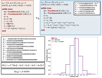
Figure 1. The probabilistic loop in the top left panel encodes the Taylor rule (Taylor, 1993), an equation that prescribes a value for the short-term interest rate based on a target inflation rate and the gross domestic product. The program uses a non-polynomial function (log) in the loop body to update the continuous-state variable ($i$). The top right panel contains the Prob-Solvable loop (with polynomial updates) obtained by approximating the log function using polynomial chaos expansion (up to $5$th degree). In the bottom left, we compute the expected interest rate ($\mathbb{E}[i_{n}]$) as a closed-form expression in loop iteration $n$ using the Prob-solvable loop and evaluate it at $n=20$. In the bottom right panel, we compare the true and estimated distributions for a fixed iteration (we sample the loop $10^{6}$ times at iteration $n=20$).

Figure 2. On the left is a probabilistic loop modeling the behavior of a turning vehicle (Sankaranarayanan et al., 2020) using non-polynomial (cos, sin) updates in the loop body. On the top right is the exact expected position $(x_{n},y_{n})$ and other exact expected values computed automatically in closed-form in the number of loop iterations $n$. The plot in the center contains $20$ sampled trajectories $(x_{n},y_{n})$ up to iteration $n=201$ (dashdot lines with different colors) and the approximated expected trajectory computed by averaging the sampled ones (dashed blue line). Moreover, we automatically computed the exact expected trajectory and standard deviation with our method. The solid purple line marks the exact expected trajectory. The two solid red lines mark the boundary of the region contained within $\pm$ two standard deviations of the expected trajectory.

Related Work.

Taylor series models (Revol et al., 2005; Neher et al., 2007; Chen et al., 2012) are a well-established computational tool in reachability analysis for (non-probabilistic) non-linear dynamical systems that combine the polynomial approximation of Taylor series expansion with the error intervals to over-approximate the set of dynamical trajectories for a finite time horizon. (Sankaranarayanan et al., 2020) approximates non-polynomial functions of random variables as polynomials using Taylor series expansion. Other works (Stanković, 1996; Triebel, 2001) follow a similar approach. Such approximations work well in the neighborhood of a point, requiring otherwise a polynomial with a high degree to maintain a good level of accuracy. This approach is not suitable for approximating functions with unbounded support.

Our two approaches, exact and gPCE based, have several advantages over the method proposed in (Sankaranarayanan et al., 2020). First, in contrast, to (Sankaranarayanan et al., 2020), neither of our methods is limited to a fixed iteration. Instead, we compute closed-form expressions in the number of loop iterations. Second, the interval estimates in  (Sankaranarayanan et al., 2020) become larger after a few iterations. Our exact moment calculation for the same models, involving trigonometric functions, is not affected by iteration number and is exact (i.e., incurs no error) at all iterations.

The method of (Jasour et al., 2021), which we adjusted, extended, and made compatible with Polar, concerns discrete-time stochastic nonlinear dynamical systems subjected to probabilistic uncertainties. (Jasour et al., 2021) focused on nonlinear autonomous and robotic systems where motion dynamics are described in terms of translational and rotational motions over the planning horizon. The latter naturally led to the introduction of trigonometric and mixed-trigonometric-polynomial moments in order to obtain an exact description of the moments of uncertain states. This method computes exact moments but it can only handle systems encoded in PPs, where all nonlinear transformations take standard, trigonometric, or mixed-trigonometric polynomial forms. Our approximate gPCE-based approach instead is applicable to general non-polynomial updates (e.g. containing logarithms). Furthermore, the work of (Jasour et al., 2021) only considers the computation of moments up to a fixed horizon. In contrast, for systems that can be modeled as Prob-solvable loops, both our methods provide closed-form expressions parameterized by the number of loop iterations.

Polynomial chaos expansion based methods have been extensively used for uncertainty quantification in different areas, such as engineering problems of solid and fluid mechanics (e.g. (Ghanem and Spanos, 1991; Foo et al., 2007; Hou et al., 2006)), computational fluid dynamics (e.g., (Knio and Maître, 2006)), flow through porous media (Ghanem and Dham, 1998; Ghanem, 1998), thermal problems (Hien and Kleiber, 1997), analysis of turbulent velocity fields (Chorin, 1974; Meecham and Jeng, 1968), differential equations (e.g., (Wan and Karniadakis, 2005; Xiu and Karniadakis, 2002)), and, more recently, geosciences and meteorology (e.g., (Formaggia et al., 2013; Giraldi et al., 2017; Denamiel et al., 2020)).

Outline.

Sec. 2 provides the necessary background on Prob-solvable Loops and the theory of general Polynomial Chaos Expansion (gPCE). Sec. 3 introduces our gPCE-based approximation method presenting the conditions that are necessary to accurately approximate general non-polynomial updates in a probabilistic loop. Sec. 4 shows how to obtain a Prob-solvable loop using our approximation method and hence how to automatically compute moment-based invariants of all orders for the program state variables. Sec. 5 presents the exact method leveraging the theory in (Jasour et al., 2021) to compute the exact moments of PPs with trigonometric and exponential updates. Sec. 6 evaluates the accuracy and feasibility of the proposed approaches over several benchmarks comparing them with the state-of-the-art. We conclude in Sec. 7.

2. Preliminaries

We assume the reader to be familiar with basic probability theory. For more details, we refer to (Durrett, 2019).

2.1. Prob-Solvable Loops

(Bartocci et al., 2019) defined the class of Prob-solvable loops for which moments of all orders of program variables can be computed symbolically: given a Prob-solvable loop and a program variable $x$, their method computes a closed-form solution for $\mathbb{E}(x_{n}^{k})$ for arbitrary $k\in{\mathbb{N}}$, where $n$ denotes the $n$th loop iteration. Prob-solvable loops are restricted to polynomial variable updates.

Definition 2.1 (Prob-solvable loops (Bartocci et al., 2019)).

Let $m\in{\mathbb{N}}$ and $x_{1},\ldots x_{m}$ denote real-valued program variables. A Prob-solvable loop with program variables $x_{1},\ldots x_{m}$ is a loop of the form

$$I;\texttt{ while true: }U\texttt{ end},\quad\text{such that}$$

• $I$ is a sequence of initial assignments over a subset of $\{x_{1},\ldots,x_{m}\}$. The initial values of $x_{i}$ can be drawn from a known distribution. They can also be real constants.

• $U$ is the loop body and a sequence of $m$ random updates, each of the form,

  $$x_{i}=\textit{Dist}\quad\text{or}\quad x_{i}=a_{i}x_{i}+P_{i}(x_{1},\dots x_{i-1}),$$

  where $a_{i}\in$, $P_{i}\in[x_{1},\ldots,x_{i-1}]$ is a polynomial over program variables $x_{1},\ldots,x_{i-1}$ and Dist is a random variable whose distribution is independent of program variables with computable moments. $a_{i}$ and the coefficients in $P_{i}$ can be random variables with the same constraints as for Dist.

The syntax of Prob-solvable loops as defined in Definition 2.1 is restrictive. For instance, an assignment for a variable $x_{i}$ must not reference variables $x_{j}$ with $j>i$. Hence, the structural dependencies among program variables are acyclic. Some of these syntactical restrictions were lifted in a later work (Moosbrugger et al., 2022) to support distributions depending on program variables, if-statements, and linear cyclic dependencies. The latter means that polynomial assignments can be of the form $x_{i}=L_{i}(x_{1},\dots,x_{n})+P_{i}(x_{1},\dots x_{i-1})$, where $P_{i}$ is a polynomial, and $L_{i}$ is a linear function, as long as all program variables in $L_{i}(x_{1},\dots,x_{n})$ with non-zero coefficient depend only linearly on $x_{i}$. In this work, we utilize this relaxation and allow for linear cyclic dependencies in Prob-solvable loops.

Many real-life systems exhibit non-polynomial dynamics and require more general updates, such as, for example, trigonometric or exponential functions. In this work, we develop two methods – one approximate, one exact – that allow the modeling of non-polynomial assignments in probabilistic loops by polynomial assignments. Doing so allows us to use the Prob-solvable loop based methods in (Bartocci et al., 2019; Moosbrugger et al., 2022) to compute the moments of the stochastic components of a much broader class of systems. Our method for exact moment derivation for probabilistic loops with non-polynomial functions builds upon Prob-solvable loops. In contrast, our PCE-based approach, described in the following sections, is not limited to Prob-solvable and can be used in more general probabilistic loops. The only requirement is that the loops satisfy the conditions in Section 3.1.

2.2. Polynomial Chaos Expansion

Polynomial chaos expansion (PCE) (Ernst, Oliver G. et al., 2012; Xiu and Karniadakis, 2002) recovers a random variable in terms of a linear combination of functionals whose entries are known random variables, sometimes called germs, or, basic variables. Let $(\Omega,\Sigma,\mathbb{P})$ be a probability space, where $\Omega$ is the set of elementary events, $\Sigma$ is a $\sigma$-algebra of subsets of $\Omega$, and $\mathbb{P}$ is a probability measure on $\Sigma$. Suppose $X$ is a real-valued random variable defined on $(\Omega,\Sigma,\mathbb{P})$, such that

(1) $$\mathbb{E}(X^{2}) =\int_{\Omega}X^{2}(\omega)d\mathbb{P}(\omega)<\infty.$$

The space of all random variables $X$ satisfying (1) is denoted by $L^{2}(\Omega,\Sigma,\mathbb{P})$. That is, the elements of $L^{2}(\Omega,\Sigma,\mathbb{P})$ are real-valued random variables defined on $(\Omega,\Sigma,\mathbb{P})$ with finite second moments. If we define the inner product as $\mathbb{E}(XY)=(X,Y)=\int_{\Omega}X(\omega)Y(\omega)d\mathbb{P}(\omega)$ and norm $||X||=\sqrt{\mathbb{E}(X^{2})}=\sqrt{\int_{\Omega}X^{2}(\omega)d\mathbb{P}(\omega)}$, then $L^{2}(\Omega,\Sigma,\mathbb{P})$ is a Hilbert space; i.e., an infinite dimensional linear space of functions endowed with an inner product and a distance metric. Elements of a Hilbert space can be uniquely identified by their coordinates with respect to an orthonormal basis of functions, in analogy with Cartesian coordinates in the plane. Convergence with respect to the norm $||\cdot||$ is called mean-square convergence. A particularly important feature of a Hilbert space is that when the limit of a sequence of functions exists, it belongs to the space.

The elements in $L^{2}(\Omega,\Sigma,\mathbb{P})$ can be classified in two groups: basic and generic random variables, which we want to decompose using the elements of the first set of basic variables. (Ernst, Oliver G. et al., 2012) showed that the basic random variables that can be used in the decomposition of other functions have finite moments of all orders with continuous probability density functions (pdfs).

The $\sigma$-algebra generated by the basic random variable $Z$ is denoted by $\sigma(Z)$. Suppose we restrict our attention to decompositions of a random variable $X=g(Z)$, where $g$ is a function with $g(Z)\in L^{2}(\Omega,\sigma(Z),\mathbb{P})$, and the basic random variable $Z$ determines the class of orthogonal polynomials $\{\phi_{i}(Z),i\in\mathbb{N}\}$,

(2) $$\left<\phi_{i}(Z),\phi_{j}(Z)\right> =\int_{\Omega}\phi_{i}(Z(\omega))\phi_{j}(Z(\omega))d\mathbb{P}(\omega)=\int\phi_{i}(x)\phi_{j}(x)f_{Z}(x)dx=\begin{cases}1&i=j\\ 0&i\neq j\end{cases}$$

where $f_{Z}$ denotes the pdf of $Z$. The set $\{\phi_{i}(Z),i\in\mathbb{N}\}$ is a polynomial chaos basis.

If $Z$ is normal with mean zero, the Hilbert space $L^{2}(\Omega,\sigma(Z),\mathbb{P})$ is called Gaussian and the related set of polynomials is represented by the family of Hermite polynomials (see, for example, (Xiu and Karniadakis, 2002)) defined on the whole real line. Hermite polynomials form a basis of $L^{2}(\Omega,\sigma(Z),\mathbb{P})$. Therefore, every random variable $X$ with finite second moment can be approximated by the truncated PCE

(3) $$X^{(d)} =\sum_{i=0}^{d}c_{i}\phi_{i}(Z),$$

for suitable coefficients $c_{i}$ that depend on the random variable $X$. The truncation parameter $d$ is the highest polynomial degree in the expansion. Since the polynomials are orthogonal,

(4) $$c_{i} =\frac{1}{||\phi_{i}||^{2}}\left<X,\phi_{i}\right>=\frac{1}{||\phi_{i}||^{2}}\left<g,\phi_{i}\right>=\frac{1}{||\phi_{i}||^{2}}\int g(x)\phi_{i}(x)f_{Z}(x)dx.$$

The truncated PCE of $X$ in (3) converges in mean square to $X$ (Ernst, Oliver G. et al., 2012, Sec. 3.1). The first two moments of (3) are determined by $\mathbb{E}(X^{(d)})=c_{0},$ and $\mathbb{V}\mathrm{ar}(X^{(d)})=\sum_{i=1}^{d}c_{i}^{2}||\phi_{i}||^{2}.$

Representing a random variable by a series of Hermite polynomials in a countable sequence of independent Gaussian random variables is known as Wiener–Hermite polynomial chaos expansion. In applications of Wiener–Hermite PCEs, the underlying Gaussian Hilbert space is often taken to be the space spanned by a sequence $\{Z_{i},i\in\mathbb{N}\}$ of independent standard Gaussian basic random variables; i.e., $Z_{i}\sim\mathcal{N}(0,1)$. For computational purposes, the countable sequence $\{Z_{i},i\in\mathbb{N}\}$ is restricted to a finite number $k\in\mathbb{N}$ of random variables. The Wiener–Hermite PCE converges for random variables with finite second moment. Specifically, for any random variable $X\in L^{2}(\Omega,\sigma(\{Z_{i},i\in\mathbb{N}\}),\mathbb{P})$, the approximation (3) satisfies

(5) $$X_{k}^{(d)}=\sum_{i=0}^{d}a_{i}\phi_{i}(Z_{1},\ldots,Z_{k}) \to X\quad\mbox{as }d,k\to\infty$$

in mean-square convergence (see (Ernst, Oliver G. et al., 2012)). The distribution of $X$ can be quite general; e.g., discrete, singularly continuous, absolutely continuous as well as of mixed type.

3. Polynomial Chaos Expansion Algorithm

3.1. Random Function Representation

In this section, we state the conditions under which the estimated polynomial is an unbiased and consistent estimator and has exponential convergence rate. Suppose $k$ continuous random variables $Z_{1},\ldots,Z_{k}$ are used to introduce stochasticity in a PP with corresponding cumulative distribution functions (cdfs) $F_{Z_{i}}$, $i=1,\ldots,k$. Also, suppose all $k$ distributions have probability density functions, and let ${\mathbf{Z}}=(Z_{1},\ldots,Z_{k})$ with cdf $F_{{\mathbf{Z}}}$. We assume that the elements of ${\mathbf{Z}}$ satisfy the following conditions:

• $Z_{i}$, $i=1,\ldots,k$, are independent.

• We consider functions $g$ such that $g({\mathbf{Z}})\in L^{2}(\mathcal{Q},F_{\mathbf{Z}})$, where $\mathcal{Q}$ is the support of the joint distribution of ${\mathbf{Z}}=(Z_{1},\ldots,Z_{k})$.

• All random variables $Z_{i}$ have distributions that are uniquely characterized by their moments.

Under condition (A), the joint cdf of the components of ${\mathbf{Z}}$ is $F_{{\mathbf{Z}}}=\prod_{i=1}^{k}F_{Z_{i}}$. To ensure the construction of unbiased estimators with optimal exponential convergence rate (see (Xiu and Karniadakis, 2002), (Ernst, Oliver G. et al., 2012)) in the context of probabilistic loops, we further introduce the following assumptions:

• $g$ is a function of a fixed number of basic variables (arguments) over all loop iterations.

• If ${\mathbf{Z}}(j)=(Z_{1}(j),\ldots,Z_{k}(j))$ is the stochastic argument of $g$ at iteration $j$, then $F_{Z_{i}(j)}(x)=F_{Z_{i}(l)}(x)$ for all pairs of iterations $(j,l)$ and $x$ in the support of $F_{Z_{i}}$.

If Conditions (D) and (E) are not met, then the polynomial coefficients in the PCE need be computed for each loop iteration individually to ensure optimal convergence rate. It is straightforward to show the following proposition.

Proposition 3.1.

If ${\mathbf{Z}}=(Z_{1},\ldots,Z_{k_{1}})$, ${\mathbf{Y}}=(Y_{1},\ldots,Y_{k_{2}})$ satisfy conditions (A), (C) and (E) and are mutually independent, and functions $g$ and $h$ satisfy conditions (B) and (D), then their sum, $g({\mathbf{Z}})+h({\mathbf{Y}})$, and product, $g({\mathbf{Z}})\cdot h({\mathbf{Y}})$, also satisfy conditions (B) and (D).

Figure 3. Illustration of PCE algorithm

3.2. PCE Algorithm

Let $Z_{1},\ldots,Z_{k}$ be independent continuous random variables, with respective cdfs $F_{i}$, satisfying conditions (A), (B) and (C). Then, ${\mathbf{Z}}=(Z_{1},\ldots,Z_{k})^{T}$ has cdf ${\mathbf{F}}_{{\mathbf{Z}}}=\prod_{i=1}^{k}F_{i}$. Let $\mathcal{Q}$ denote the support of ${\mathbf{F}}_{{\mathbf{Z}}}$. The function $g:^{k}\to$, with $g\in L^{2}(\mathcal{Q},{\mathbf{F}})$, can be approximated with the truncated orthogonal polynomial expansion, as described in Fig. 3,

(6) $$g({\mathbf{Z}}) \approx\hat{g}({\mathbf{Z}})=\sum_{\begin{subarray}{c}d_{i}\in\{0,\ldots,\bar{d}_{i}\},\\ i=1,\ldots,k\end{subarray}}c(d_{1},\ldots,d_{k})z_{1}^{d_{1}}\cdots z_{k}^{d_{k}}=\sum_{j=1}^{L}c_{j}\prod\limits_{i=1}^{k}\bar{p}_{i}^{d_{ji}}(z_{i}),$$

where

• $\bar{p}_{i}^{d_{ji}}(z_{i})$ is a polynomial of degree $d_{ji}$, and belongs to the set of orthogonal polynomials with respect to $F_{Z_{i}}$ that are calculated with the Gram-Schmidt orthogonalization procedure;

• $\bar{d}_{i}=\max\limits_{j}(d_{ji})$ is the highest degree of the univariate orthogonal polynomial, for $i=1,\ldots,k$;

• $L=\prod\limits_{i=1}^{k}(1+\bar{d}_{i})$ is the total number of multivariate orthogonal polynomials and equals the truncation constant;

• $c_{j}$ are the Fourier coefficients.

The Fourier coefficients are calculated using

(7) $$c_{j} =\int\limits_{\mathcal{Q}}g(z_{1},...,z_{k})p_{i}^{d_{ji}}(z_{i})d{\mathbf{F}}=\idotsint\limits_{\mathcal{Q}}g(z_{1},...,z_{k})\left(\prod\limits_{i=1}^{k}\bar{p}_{i}^{d_{ji}}(z_{i})\right)dF_{Z_{k}}...dF_{Z_{1}},$$

by Fubini’s theorem.

Example 3.2.

Returning to the Turning vehicle model in Fig. 2, the non-polynomial functions to approximate are $g_{1}=cos$ and $g_{2}=sin$ from the updates of program variables $y,x$, respectively. In both cases, we only need to consider a single basic random variable, $Z\sim\mathcal{N}(0,0.01)$ ($\psi$ in Fig. 2).

Using polynomials of degree up to $5$, (6) has the following form for the two functions,

(8) $$\hat{g}_{1}(z)=cos(\psi)=a_{0}+a_{1}\psi+...+a_{5}\psi^{5}$$

and

(9) $$\hat{g}_{2}(z)=sin(\psi)=b_{0}+b_{1}\psi+...+b_{5}\psi^{5}.$$

We compute the coefficients $a_{i},b_{i}$ in equations (8)-(9) using (7) to obtain the values shown in Fig. 2.

Example 3.3.

Consider the function $g(x,y)=\sqrt{x^{2}+y^{2}}$, where $x\sim Uniform(-1,1)$ and $y$ has pdf $f_{y}=0.75(1-y^{2})$ supported on $\left[-1,1\right]$. Up to degree 2, the basis elements in the PC expansion are element-wise products of the univariate orthogonal polynomials

$$p^{0}_{x}(x)=1,\quad p^{0}_{y}(y)=1,p^{1}_{x}(x)=\sqrt{3}x,\quad p^{1}_{y}(y)=\sqrt{5}y,$$

$$p^{2}_{x}(x)=1.5\sqrt{5}x^{2}-0.5\sqrt{5},\,p^{2}_{y}(y)=1.25\sqrt{14}y^{2}-0.25\sqrt{14}.$$

The corresponding PCE polynomial basis elements are

$$p^{00}_{xy}(x,y)=1,\quad p^{02}_{xy}(x,y)=1.25\sqrt{14}y^{2}-0.25\sqrt{14},\quad p^{20}_{xy}(x,y)=1.5\sqrt{5}x^{2}-0.5\sqrt{5},$$

$$p^{22}_{xy}(x,y)=1.875\sqrt{70}x^{2}y^{2}-0.375\sqrt{70}x^{2}-0.625\sqrt{70}y^{2}+0.125\sqrt{70},$$

with corresponding non-zero Fourier coefficients $c_{00}=0.677408,c_{02}=0.154109,c_{20}=0.216390$, and $c_{22}=-0.040153.$ The resulting estimator is

$$\hat{g}(x,y)=\sum\limits_{(i,j)=(0,0)}^{(2,2)}c_{i,j}p^{ij}_{xy}(x,y)=-0.629900x^{2}y^{2}+0.851774x^{2}+0.930747y^{2}+0.249327.$$

Complexity.

Assuming the expansion is carried out up to the same polynomial degree $d$ for each basic variable, $\bar{d}_{i}=d$, $\forall i=1,...,k$. This implies $d=\sqrt[k]{L}-1$. The complexity of the scheme is $\mathcal{O}(sd^{2}k+s^{k}d^{k})$, where $\mathcal{O}(s)$ is the complexity of computing univariate integrals.

The complexity of our approximation scheme consists of of two parts: (1) the orthogonalization process and (2) the calculation of coefficients. Regarding (1), we orthogonalize and normalize $k$ sets of $d$ basic linearly independent polynomials via the Gram-Schmidt process. For degree $d{=}1$, we need to calculate one integral, the inner product with the previous polynomial. Additionally, we need to compute one more integral, the norm of itself (for normalization). For each subsequent degree $d^{\prime}$, we must calculate $d^{\prime}$ additional new integrals. The computation of each integral has complexity $\mathcal{O}(s)$. Regarding (2), the computation of the coefficients requires calculating $L{=}(d{+}1)^{k}$ integrals with $k$-variate functions as integrands.

We define the approximation error to be

(10) $$se(\hat{g})=\sqrt{\int\limits_{\mathcal{Q}}\left(g(z_{1},...,z_{k})-\hat{g}(z_{1},...,z_{k})\right)^{2}dF_{Z_{1}}\ldots dF_{Z_{k}}}$$

since $\mathbb{E}(\hat{g}(Z_{1},...,Z_{k}))=g(Z_{1},\cdots,Z_{k})$ by construction.

The implementation of this algorithm may become challenging when the random functions have complicated forms and the number of parametric uncertainties is large. In this case, the calculation of the PCE coefficients involves high dimensional integration, which may prove difficult and time prohibitive for real-time applications (Son and Du, 2020).

4. Prob-Solvable Loops for General Non-Polynomial Functions

PCE allows incorporating non-polynomial updates into Prob-solvable loop programs and use the algorithm in (Bartocci et al., 2019) and exact tools, such as Polar (Moosbrugger et al., 2022), for moment (invariant) computation. We identify two classes of programs based on how the distributions of the generated random variables vary.

4.1. Iteration-Stable Distributions of Random Arguments

Let $\mathcal{P}$ be an arbitrary Prob-solvable loop and suppose that a (non-basic) state variable $x\in\mathcal{P}$ has a non-polynomial $L^{2}$-type update $g({\mathbf{Z}})$, where ${\mathbf{Z}}=(Z_{1},\ldots,Z_{k})^{T}$ is a vector of (basic) continuous, independent, and identically distributed random variables across iterations. That is, if $f_{Z_{j}(n)}$ is the pdf of the random variable $Z_{j}$ in iteration $n$, then $f_{Z_{j}(n)}\equiv f_{Z_{j}(n^{\prime})}$, for all iterations $n,n^{\prime}$ and $j=1,\ldots,k$. The basic random variables $Z_{1},\ldots,Z_{k}$ and the update function $g$ satisfy conditions (A)–(E) in Section 3.1. For the class of Prob-solvable loops where all variables with non-polynomial updates satisfy these conditions, the computation of the Fourier coefficients in the PCE approximation (6) can be carried out as explained in Section 3.2. In this case, the convergence rate is optimal.

4.2. Iteration Non-Stable Distribution of Random Arguments

Let $\mathcal{P}$ be an arbitrary Prob-solvable loop and suppose that a state variable $x\in\mathcal{P}$ has a non-polynomial $L^{2}$-type update $g({\mathbf{Z}})$, where ${\mathbf{Z}}=(Z_{1},\ldots,Z_{k})^{T}$ is a vector of continuous independent but not necessarily identically distributed random variables across iterations. For this class of Prob-solvable loops, conditions (A)–(C) in Section 3.1 hold, but (D) and/or (E) may not be fulfilled. In this case, we can ensure optimal exponential convergence by fixing the number of loop iterations. For unbounded loops, we describe an approach converging in mean-square and establish its convergence rate next.

Conditional estimator given number of iterations.

Let $N$ be an a priori fixed finite integer, representing the maximum iteration number. The set $\{1,\ldots,N\}$ is a finite sequence of iterations for the Prob-solvable loop $\mathcal{P}$.

Iterations are executed sequentially for $n=1,\ldots,N$, which allows the estimation of the final functional that determines the target state variable at each iteration $n\in\{1,\ldots,N\}$ and its set of supports. Knowing these features, we can carry out $N$ successive expansions. Let $P(n)$ be a PCE of $g({\mathbf{Z}})$ for iteration $n$. We introduce an additional program variable $c$ that counts the loop iterations. The variable $c$ is initialized to $0$ and incremented by $1$ at the beginning of every loop iteration. The final estimator of $g({\mathbf{Z}})$ can be represented as

(11) $$\hat{g}({\mathbf{Z}})=\sum\limits_{n=1}^{N}P(n)\left[\prod\limits_{j=1,j\neq n}^{N}\frac{(c-j)}{n-j}\right].$$

Replacing non-polynomial functions with (11) results in a program with only polynomial-type updates and constant polynomial structure; that is, polynomials with coefficients that remain constant across iterations. Moreover, the estimator is unbiased with optimal exponential convergence on the set of iterations $\{1,\ldots,N\}$ (Xiu and Karniadakis, 2002).

Unconditional estimator.

Here the iteration number is unbounded. Without loss of generality, we consider a single basic random variable $Z$; that is, $k{=}1$. The function $g(Z)$ is scalar-valued and can be represented as a polynomial of nested $L^{2}$ functions, which depend on polynomials of the argument variable. Each nested functional argument is expressed as a sum of orthogonal polynomials yielding the final estimator, which is itself a polynomial.

Since PCE converges to the function it approximates in mean-square (see (Ernst, Oliver G. et al., 2012)) on the whole interval (argument’s support), PCE converges on any sub-interval of the support of the argument in the same sense.

Let us consider a function $g$ with a sufficiently large domain and a random variable $Z$ with known distribution and support. For example, $g(Z)=e^{Z}$, with $Z\sim N(\mu,\sigma^{2})$. The domain of $g$ and the support of $Z$ are the real line. We can expand $g$ into a PCE with respect to the distribution of $Z$ as

(12) $$g(Z) =\sum\limits_{i=0}^{\infty}c_{i}p_{i}(Z).$$

The distribution of $Z$ is reflected in the polynomials in (12). Specifically, $p_{i}$, for $i=0,1,\ldots$, are Hermite polynomials of special type in that they are orthogonal (orthonormal) with respect to $N(\mu,\sigma^{2})$. They also form an orthogonal basis of the space of $L^{2}$ functions. Consequently, any function in $L^{2}$ can be estimated arbitrarily closely by these polynomials. In general, any continuous distribution with finite moments of all orders and sufficiently large support can also be used as a model for basic variables in order to construct a basis for $L^{2}$ (see (Ernst, Oliver G. et al., 2012)).

Now suppose that the distribution of the underlying variable $Z$ is unknown with pdf $f_{Z}(z)$ that is continuous on its support $\left[a,b\right]$. Then, there exists another basis of polynomials, $\{q_{i}\}_{i=0}^{\infty}$, which are orthogonal on the support $\left[a,b\right]$ with respect to the pdf $f_{Z}$. Then, on the interval $\left[a,b\right]$, $g(Z)=\sum_{i=0}^{\infty}k_{i}q_{i}(Z)$, and $\mathbb{E}_{f}\left[g(Z)\right]=\mathbb{E}_{f}\left[\sum_{i=0}^{M}k_{i}q_{i}(Z)\right]$, $\forall M\geq 0$.

Since $\left[a,b\right]\subset$, the expansion $\sum_{i=0}^{\infty}c_{i}p_{i}(Z)$ converges in mean-square to $g(Z)$ on $\left[a,b\right]$. In the limit, we have $g(Z)=\sum_{i=0}^{\infty}c_{i}p_{i}(Z)$ on the interval $\left[a,b\right]$. Also, $\mathbb{E}_{f}\left(g(Z)\right)=\mathbb{E}_{f}\left(\sum_{i=0}^{\infty}c_{i}p_{i}(Z)\right)$ for the true pdf $f$ on $\left[a,b\right]$. In general, though, it is not true that $\mathbb{E}_{f}\left(g(Z)\right)=\mathbb{E}_{f}\left(\sum_{i=0}^{M}c_{i}p_{i}(Z)\right)$ for any arbitrary $M\geq 0$ and any pdf $f_{Z}(z)$ on $\left[a,b\right]$, as the estimator is biased.

To capture this discrepancy, we define the approximation error as

(13) $$e(M) =\mathbb{E}_{f}\left(g(Z)-\sum\limits_{i=0}^{M}c_{i}p_{i}(Z)\right)^{2}=\mathbb{E}_{f}\left(\sum\limits_{i=M+1}^{\infty}c_{i}p_{i}(Z)\right)^{2}.$$

Computation of error bound.

Assume the true pdf $f_{Z}$ of $Z$ is supported on $\left[a,b\right]$. Also, assume the domain of $g$ is $\mathbb{R}$. The random function $g(Z)$ has PCE on the whole real line based on Hermite polynomials $\{p_{i}(Z)\}_{i=0}^{\infty}$ that are orthogonal with respect to the standard normal pdf $\phi$. The truncated expansion estimate of (12) with respect to a normal basic random variable is

(14) $$\hat{g}(Z) =\sum\limits_{i=0}^{M}c_{i}p_{i}(Z).$$

We compute an upper bound for the approximation error for our scheme in Theorem (4.1).

Theorem 4.1.

Suppose $Z$ has density $f_{Z}$ supported on $[a,b]$, $g:\to$ is in $L^{2}$, and $\phi$ denotes the standard normal pdf. Under (12) and (14),

$$\left\|g(Z)-\hat{g}(Z)\right\|_{f}^{2} =\int_{a}^{b}\left(g(z)-\hat{g}(z)\right)^{2}f_{Z}(z)dz$$

(15) $$\leq\left(\frac{2}{\min{(\phi(a),\phi(b))}}+1\right)\mathbb{V}\mathrm{ar}_{\phi}\left(g(Z)\right).$$

The upper bound in (15) depends only on the support of $f_{Z}$ and the function $g$. If $Z$ is standard normal ($f_{Z}=\phi$), then the upper bound in (15) equals $\mathbb{V}\mathrm{ar}_{\phi}(g(Z))$. We provide the proof of Theorem 4.1 in Appendix A.

Remark 0.

The approximation error inequality in (Mühlpfordt et al., 2018, Lemma 1),

(16) $$\left\|{g(Z)-\sum_{i=0}^{T}c_{i}p_{i}(Z)}\right\|\leq\frac{\|g(Z)^{(k)}\|}{\prod_{i=0}^{k-1}\sqrt{T-i+1}},$$

is a special case of Theorem 4.1 when $Z\sim\mathcal{N}(0,1)$ and $f_{Z}=\phi$, and the polynomials $p_{i}$ are Hermite. In this case, the left hand side of (16) equals $\sqrt{\sum_{i=n+1}^{\infty}c_{i}^{2}}$.

Although Theorem 4.1 is restricted to distributions with bounded support, the approximation in (14) also converges for distributions with unbounded support.

5. Exact Moment Derivation

In Sections 3 and 4, we combined PCE with the Prob-solvable loop algorithm of (Moosbrugger et al., 2022; Bartocci et al., 2019) to compute PCE approximations of the moments of the distributions of the random variables generated in a probabilistic loop. In this section, we develop a method for the derivation of the exact moments of probabilistic loops that comply with a specified loop structure and functional assignments. (Bartocci et al., 2019), and later (Moosbrugger et al., 2022), introduce a technique for exact moment computation for Prob-solvable loops without non-polynomial functions. Prob-solvable loops support common probability distributions $F$ with constant parameters and program variables $x$ with specific polynomial assignments (cf. Section 2). In Section 5.1, we first show how to compute $\mathbb{E}(h(F)^{k})$ where $h$ is the exponential or a trigonometric function. In Section 5.2, we describe how to incorporate trigonometric and exponential updates of program variables $x$ into the Prob-solvable loop setting.

5.1. Trigonometric and Exponential Functions for Distributions

The first step in supporting trigonometric and exponential functions in Prob-solvable loops is to understand how to compute the expected values of random variables that are trigonometric and exponential functions of random variables with known distributions. Due to the polynomial arithmetic supported in Prob-solvable loops, non-polynomial functions of random variables can be mixed via multiplication in the resulting program. We adopt the results from (Jasour et al., 2021) providing a formula for the expected value of mixed trigonometric polynomials of distributions, given the distributions’ characteristic functions.

Definition 5.1.

We call $p(x)$ a standard polynomial of order $d\in{\mathbb{N}}$ if

$$p(x)=\sum_{k=0}^{d}\alpha_{k}x^{k},$$

with coefficients $\alpha_{k}\in$. Further, $p(x)$ is defined to be a mixed trigonometric polynomial if it is a mixture of a standard polynomial with trigonometric functions of the form

$$p(x)=\sum_{k=0}^{d}\alpha_{k}x^{b_{k}}\cdot cos^{c_{k}}(x)\cdot sin^{s_{k}}(x),$$

with $b_{k},c_{k},s_{k}\in{\mathbb{N}}$ and coefficients $\alpha_{k}\in$ (Jasour et al., 2021).

Following (Jasour et al., 2021), we define the mixed-trigonometric-polynomial moment of order $\alpha$ for a random variable $X$ as

(17) $$m_{X^{\alpha_{1}}c_{X}^{\alpha_{2}}s_{X}^{\alpha_{3}}} =\mathbb{E}\left[X^{\alpha_{1}}\cos^{\alpha_{2}}(X)\sin^{\alpha_{3}}(X)\right],$$

where $(\alpha_{1},\alpha_{2},\alpha_{3})\in{\mathbb{N}}^{3}$ such that $\alpha=\sum_{k=1}^{3}\alpha_{k}$. When the characteristic function of the random variable $X$ is known, Lemma 4 in (Jasour et al., 2021), together with the linearity of the expectation operator, provides the computation rule for (17):

(18) $$m_{X^{\alpha_{1}}c_{X}^{\alpha_{2}}s_{X}^{\alpha_{3}}}=\frac{1}{i^{\alpha_{1}+\alpha_{3}}2^{\alpha_{2}+\alpha_{3}}}\times\sum\limits_{(k_{1},k_{2})=(0,0)}^{(\alpha_{2},\alpha_{3})}\binom{\alpha_{2}}{k_{1}}\binom{\alpha_{3}}{k_{2}}(-1)^{\alpha_{3}-k_{2}}\frac{d^{\alpha_{1}}}{dt^{\alpha_{1}}}\Phi_{X}(t)\bigg{|}_{t=2(k_{1}+k_{2})-\alpha_{2}-\alpha_{3}}.$$

Example 5.2.

Let ${\mathbf{X}}\sim\mathcal{N}(0,1)$. Its characteristic function is $\Phi_{X}(t)=\exp(-0.5t^{2})$ and $\Phi^{\prime}_{X}(t)=-t\exp(-0.5t^{2})$. Then,

$$\mathbb{E}\left[X\sin(X)\cos(X)\right] =\frac{1}{i^{2}2^{2}}\left(-\Phi^{\prime}_{X}(-2)+\Phi^{\prime}_{X}(0)-\Phi^{\prime}_{X}(0)+\Phi^{\prime}_{X}(2)\right)=\exp(-2).$$

To support exponential functions in Prob-solvable loops, we define mixed exponential polynomials as

$$p(x)=\sum_{k=0}^{d}\alpha_{k}x^{b_{k}}\exp^{e_{k}}(x),$$

with $b_{k},e_{k}\in{\mathbb{N}}$ and coefficients $\alpha_{k}\in$. Lemma 5.3 obtains a computational rule for moments of mixed exponential polynomials, provided they exist, in terms of the moment-generating function of the random variable $X$.

Lemma 5.3.

Let $X$ be a random variable with moment-generating function $\mathcal{M}_{X}(t)=\mathbb{E}\left[\exp(tX)\right]$. Suppose $\alpha_{1},\alpha_{2}\in{\mathbb{N}}$, and let $\alpha=\alpha_{1}+\alpha_{2}$. If the mixed-exponential-polynomial moment of order $\alpha$ exists, it can be computed using the following formula

(19) $$m_{X^{\alpha_{1}}e^{\alpha_{2}}_{X}} =\mathbb{E}\left[X^{\alpha_{1}}\exp^{\alpha_{2}}(X)\right]=\frac{d^{\alpha_{1}}}{dt^{\alpha_{1}}}\mathcal{M}_{X}(t)\bigg{|}_{t=\alpha_{2}}.$$

Proof.

$$m_{X^{\alpha_{1}}e^{\alpha_{2}}_{X}}=\mathbb{E}\left[X^{\alpha_{1}}\exp^{\alpha_{2}}(X)\right]=\mathbb{E}\left[\frac{d^{\alpha_{1}}}{dt^{\alpha_{1}}}\exp(tX)\bigg{|}_{t=\alpha_{2}}\right]=\frac{d^{\alpha_{1}}}{dt^{\alpha_{1}}}\mathbb{E}\left[\exp(tX)\right]\bigg{|}_{t=\alpha_{2}}=\frac{d^{\alpha_{1}}}{dt^{\alpha_{1}}}\mathcal{M}_{X}(t)\bigg{|}_{t=\alpha_{2}}.$$

∎

Example 5.4.

Suppose $X\sim\mathcal{N}(0,1)$ with moment generating function $\mathcal{M}_{X}(t)=\exp(0.5t^{2})$. Since $X\exp^{2}(X)$ is integrable with respect to the normal pdf,

$$\mathbb{E}\left[X\exp^{2}(X)\right]=\frac{d}{dt}\exp(0.5t^{2})\bigg{|}_{t=2}=t\cdot\exp(0.5t^{2})\bigg{|}_{t=2}=2\cdot\exp(2).$$

5.2. Trigonometric and Exponential Functions in Variable Updates

We now examine the presence of trigonometric and exponential functions of program variables, specifically of accumulator variables, in Prob-solvable loops.

Definition 5.5 (Accumulator).

We call a program variable $x$ an accumulator if the update of $x$ in the loop body has the form $x=x+z$, such that $z_{i}$ and $z_{i+1}$ are independent and identically distributed for all $i\geq 1$.

Consider a loop $\mathcal{P}$ with an accumulator variable $x$, updated as $x=x+z$, and a trigonometric or exponential function $h(x)$. Further, assume that the characteristic function (if $h=\sin$ or $h=\cos$) or the moment-generating function (if $h=\exp$) of $z$ is known. Note that the distribution of the variable $x$ is, in general, different in every iteration. Listing 1 gives an example of such a loop.

Listing 1: PP loop prototype

⬇

$\displaystyle z=0;\;x=0;\;y=0$

while true:

$\displaystyle z=Normal(0,1)$

$\displaystyle x=x+z$

$\displaystyle y=y+h(x)$

end

The idea now is to transform $\mathcal{P}$ into an equivalent Prob-solvable loop $\mathcal{P}^{\prime}$ such that the term $h(x)$ does not appear in $\mathcal{P}^{\prime}$. In the following, we assume, for simplicity, that first $z$ is updated in $\mathcal{P}$, then $x$, and only then $h$ is used. The following arguments are analogous if the updates are ordered differently (only the indices change). Note that we can rewrite $h(x_{t+1})$ as $h(x_{t}+z_{t+1})$.

Transforming $\exp(x)$.

In the case of $h=\exp$, we have

(20) $$\exp(x_{t+1})=\exp(x_{t}+z_{t+1})=\exp(x_{t})\exp(z_{t+1}).$$

We utilize this property and transform the program $\mathcal{P}$ into a program $\mathcal{P}^{\prime}$ by introducing an auxiliary variable $\hat{x}$ that models the value of $\exp(x)$. The update of $\hat{x}$ in the loop body succeeds the update of $x$ and is

(21) $$\hat{x}=\hat{x}\cdot\exp(z).$$

The auxiliary variable is initialized as $\hat{x}_{0}=\exp(x_{0})$. We then replace $h(x)$ by $\hat{x}$ in $\mathcal{P}$ to arrive at our transformed program $\mathcal{P}^{\prime}$. Because $z$ is identically distributed in every iteration and its moment-generating function is known, we can use the results from Section 5.1 to compute any moment of $\exp(z)$. Thus, the update in (21) is supported by Prob-solvable loops.

Transforming sine and cosine.

In the case of $h=\sin$ or $h=\cos$, applying standard trigonometric identities obtains

(22) $$\begin{split}\cos(x_{t+1})&=\cos(x_{t}+z_{t+1})=\cos(x_{t})\cos(z_{t+1})-\sin(x_{t})\sin(z_{t+1}),\\ \sin(x_{t+1})&=\sin(x_{t}+z_{t+1})=\sin(x_{t})\cos(z_{t+1})+\cos(x_{t})\sin(z_{t+1}).\end{split}$$

We introduce two auxiliary variables, $s$ and $c$, modeling the values of $\sin(x)$ and $\cos(x)$, simultaneously updated in the loop body as

(23) $$c,\;s=c\cdot\cos(z)-s\cdot\sin(z),\;s\cdot\cos(z)+c\cdot\sin(z),$$

with the initial values $s_{0}=\sin(x_{0})$ and $c_{0}=\cos(x_{0})$. We then replace $h(x)$ with $s$ or $c$ in $\mathcal{P}^{\prime}$. Again, because $z$ is identically distributed in every iteration and its characteristic function is known, we can use the results from Section 5.1 to compute any moment of $\sin(z)$ and $\cos(z)$. Thus, the update in (23) is supported in Prob-solvable loops.

Example 5.6.

Listings 2 and 3 show the program from Listing 1 with $h=\exp$ and $h=\cos$, respectively, rewritten as equivalent Prob-solvable loops. The program in Listing 2 has linear circular variable dependencies due to the variables $c$ and $s$.

Listing 2: PP prototype equivalent – cos

⬇

$\displaystyle z=0;\;x=0;\;c=cos(z);\;s=sin(z);\;y=0$

while true:

$\displaystyle z=Normal(0,1)$

$\displaystyle x=x+z$

$\displaystyle c,\hskip 5.69046pts=c\cdot\cos(z)-s\cdot\sin(z),\hskip 5.69046pts\cdot\cos(z)+c\cdot\sin(z)$

$\displaystyle y=y+c$

end

Listing 3: PP prototype equivalent – exp

⬇

$\displaystyle z=0;\;x=0;\;\hat{x}_{i}=exp(z);\;y=0$

while true:

$\displaystyle z=Normal(0,1)$

$\displaystyle x=x+z$

$\displaystyle\hat{x}_{i}=\hat{x}_{i}\cdot\exp(z)$

$\displaystyle y=y+\hat{x}_{i}$

end

6. Evaluation

We evaluate our PCE-based method for moment approximation and our exact moment derivation approach on eleven benchmarks. The set of benchmarks consists of those in (Kofnov et al., 2022), five additional benchmarks from (Jasour et al., 2021), and a probabilistic loop modeling stochastic exponential decay. The benchmark Walking Robot in (Jasour et al., 2021) is the same as the Rimless wheel walker in (Kofnov et al., 2022).

We apply our PCE-based method to approximate non-polynomial functions. This transforms all benchmark programs into Prob-solvable loops, which allows using the static analysis tool Polar (Moosbrugger et al., 2022) to compute the moments of the program variables as a function of the loop iteration $n$.

We implemented the techniques for exact moment derivation for loops containing trigonometric or exponential polynomials, presented in Section 5, in the tool Polar. We evaluate the technique for exact moment derivation using Polar on all benchmarks satisfying the general program structure of Listing 1 in Section 5. We also compare our approximate and exact methods with the technique based on polynomial forms of (Sankaranarayanan et al., 2020). When appropriate, we applied our methods, as well as the polynomial form, on the eleven benchmark models. All experiments were run on a machine with 32 GB of RAM and a 2.6 GHz Intel i7 (Gen 10) processor.

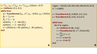
Figure 4. Probabilistic loops: (A) Rimless wheel walker (Steinhardt and Tedrake, 2012) and (B) 2D Robotic arm (Bouissou et al., 2016) (in the figure we use the inner loop as syntax sugar to keep the program compact).

Figure 5. Probabilistic loops: (A) Uncertain underwater vehicle (Pairet et al., 2022; Jasour et al., 2021), (B) Planar aerial vehicle (Steinhardt and Tedrake, 2012; Jasour et al., 2021), (C) 3D aerial vehicle (Pairet et al., 2022; Jasour et al., 2021), (D) Differential-drive mobile robot (van den Berg et al., 2011; Jasour et al., 2021), (E) Stochastic decay, (F) 3D (Mobile) Robotic arm (Jasour and Farrokhi, 2014; Jasour et al., 2021)

Taylor rule model. Central banks set monetary policy by raising or lowering their target for the federal funds rate. The Taylor rule is an equation intended to describe the interest rate decisions of central banks. The rule relates the target of the federal funds rate to the current state of the economy through the formula

(24) $$i_{t}=r^{*}_{t}+\pi_{t}+a_{\pi}(\pi_{t}-\pi^{*}_{t})+a_{y}(y_{t}-\bar{y}_{t}),$$

where $i_{t}$ is the nominal interest rate, $r^{*}_{t}$ is the equilibrium real interest rate, $r^{*}_{t}=r$, $\pi_{t}$ is inflation rate at $t$, $\pi^{*}_{t}$ is the short-term target inflation rate at $t$, $y_{t}=\log(1+Y_{t})$, with $Y_{t}$ the real GDP, and $\bar{y}_{t}=\log(1+\bar{Y}_{t})$, with $\bar{Y}_{t}$ denoting the potential real output.

Highly-developed economies grow exponentially with a sufficiently small rate (e.g., according to the World Bank, the average growth rate of the GDP in the USA in 2001-2020 equaled 1.73%). Accordingly, we set the growth rate of the potential output to 2%. We model inflation as a martingale process; that is, $\mathbb{E}_{t}\left[\pi_{t+1}\right]=\pi_{t}$, following (Atkeson and Ohanian, 2001). The Taylor rule model is described by the program in Fig. 1.

Figure 6. The approximations and their relative errors for the Taylor rule model.

Turning vehicle model. This model is described by the probabilistic program in Fig. 2. It was introduced in (Sankaranarayanan et al., 2020) and depicts the position of a vehicle, as follows. The state variables are $(x,y,v,\psi)$, where $(x,y)$ is the vehicle’s position with velocity $v$ and yaw angle $\psi$. The vehicle’s velocity is stabilized around $v_{0}=10$ m/s. The dynamics are modelled by the equations $x(t{+}1)=x(t)+\tau v\cos(\psi(t))$, $y(t{+}1)=y(t)+\tau v\sin(\psi(t))$, $v(t{+}1)=v(t)+\tau(K(v(t)-v_{0})+w_{1}(t{+}1))$, and $\psi(t{+}1)=\psi(t)+w_{2}(t{+}1)$. The disturbances $w_{1}$ and $w_{2}$ have distributions $w_{1}\sim U[-0.1,0.1]$, $w_{2}\sim N(0,0.1)$. We set $K=-0.5$, as in (Sankaranarayanan et al., 2020). Initially, the state variables are distributed as follows: $x(0)\sim U[-0.1,0.1]$, $y(0)\sim U[-0.5,-0.3]$, $v(0)\sim U[6.5,8.0]$, $\psi(0)\sim N(0,0.01)$. We allow all normally distributed parameters to take values over the entire real line, in contrast to (Sankaranarayanan et al., 2020) which could not accommodate distributions with infinite support and required the normal variables to be truncated.

Rimless wheel walker. The Rimless wheel walker (Sankaranarayanan et al., 2020; Steinhardt and Tedrake, 2012) is a system that describes a walking human. The system models a rotating wheel consisting of $n_{s}$ spokes, each of length $L$, connected at a single point. The angle between consecutive spokes is $\theta=2\pi/n_{s}$. We set $L=1$ and $\theta=\pi/6.$ This system is modeled by the program in Fig. 4 (A). For more details, we refer to (Sankaranarayanan et al., 2020).

Robotic arm model. Proposed and studied in (Bouissou et al., 2016; Sankaranarayanan, 2020; Sankaranarayanan et al., 2020), this system models the position of a 2D robotic arm. The arm moves through translations and rotations. At every step, errors in movement are modeled with probabilistic noise. The robotic arm model is described by the program in Fig. 4 (B).

Uncertain underwater vehicle. This benchmark models the movement of an underwater vehicle subject to external disturbances (Jasour et al., 2021; Pairet et al., 2022) and is encoded by the program in Fig. 5 (A). The program variables $x$ and $y$ represent the position of the vehicle in a 2D plane and $\theta$ its orientation. The external disturbances are modeled by probabilistic shocks to the velocity and the orientation of the vehicle.

Planar aerial vehicle. This benchmark was studied in (Jasour et al., 2021; Steinhardt and Tedrake, 2012) and models the vertical and horizontal movement of an aerial vehicle subject to wind disturbances. It can be written as the program in Fig. 5 (B), where the variables $x$ and $y$ represent the horizontal and vertical positions. The variable $\theta$ models the rotation around the $x$ axis. The linear velocities are captured by $v_{x}$ and $v_{y}$, and $v_{\theta}$ represents the angular velocity. The wind disturbance is modeled by the random variable $\Omega_{\theta}$. For more details, we refer to (Jasour et al., 2021).

3D aerial vehicle. This system, studied in (Jasour et al., 2021; Pairet et al., 2022), models the movement of an aerial vehicle in three-dimensional space subject to wind disturbances. The system can be written as a program as illustrated in Fig. 5 (C). The program variables $x$, $y$, and $z$ represent the position of the vehicle. The orientations around the $y$ and $z$ axis are captured by the variables $\theta$ and $\psi$, respectively. The linear and angular velocities are constant $1$. Wind disturbances are modeled by the random variables $\Omega_{\nu}$, $\Omega_{\psi}$, and $\Omega_{\theta}$. For more details, we refer to (Jasour et al., 2021).

Differential-drive mobile robot. This system models the movement of a differential-drive mobile robot with two wheels subject to external disturbances and was studied in (Jasour et al., 2021; van den Berg et al., 2011). In Fig. 5 (D) we express the Differential-drive mobile robot system as a program. The program variables $x$ and $y$ represent the robot’s position. Its orientation is captured by the variable $\theta$. The velocities are constant $1$ for the left wheel and constant $3$ for the right wheel. The random variables $\Omega_{r}$ and $\Omega_{l}$ model external disturbances. For more details, we refer to (Jasour et al., 2021).

Mobile robotic arm. The system, studied in (Jasour et al., 2021; Jasour and Farrokhi, 2014, 2010), models the uncertain position of the end-effector of a mobile robotic arm as a function of the uncertain base position and uncertain joint angles. Fig. 5 (F) shows the system as a program. The program variables $\theta_{1}$, $\theta_{2}$, and $\theta_{3}$ represent the uncertain angles of three joints. The distributions of $\theta_{1}$ and $\theta_{2}$ are uniform and normal, respectively, while $\theta_{3}$ is gamma distributed with shape parameter $1$ and scale parameter $2$. The position of the end-effector in 3D space is given by the variables $x_{E}$, $y_{E}$, and $z_{E}$. The uncertain position of the base in 3D space is modeled by three different distributions (uniform, normal, beta) in the assignments of $x_{E}$, $y_{E}$, and $z_{E}$. For more details, we refer to (Jasour et al., 2021).

Stochastic decay. The program in Fig. 5 (E) models exponential decay with a non-constant stochastic decay rate. Variable $m$ represents the total quantity subject to decay, where $m_{0}$ is the initial quantity. The decay rate $\lambda$ starts off at $0$ and changes according to a normal distribution at every time step.

Benchmark	Target	Poly form	Sim.	Exact	PCE estimate
					Deg.	Result	🕛 Runtime
Taylor rule model	$\mathbb{E}\left(i_{n}\right)$ $n{=}20$	$\times$	0.022998	$\times$	$3$ $5$ $9$	$0.02278$ $0.02295$ $0.02300$	$0.4s{+}0.5s$ $0.5s{+}5.0s$ $5.9s{+}34.6s$
Turning vehicle model	$\mathbb{E}\left(x_{n}\right)$ $n{=}20$	$\times$	15.60666	15.60760 1.9s	$3$ $5$ $9$	$14.44342$ $15.43985$ $15.60595$	$0.6s{+}3.6s$ $1.4s{+}9.2s$ $15.6s{+}16.1s$
Turning vehicle model (trunc.)	$\mathbb{E}\left(x_{n}\right)$ $n{=}20$	for deg. 2 $\left[-3\cdot 10^{5},3\cdot 10^{5}\right]$ 1057s	15.60818	15.60760 89.2s	$3$ $5$ $9$	$14.44342$ $15.43985$ $15.60595$	$0.6s{+}3.6s$ $1.4s{+}9.1s$ $15.6s{+}15.8s$
Rimless wheel walker	$\mathbb{E}\left(x_{n}\right)$ $n{=}2000$	for deg. 2 $\left[1.791,1.792\right]$ 5.42s	1.79173	1.79159 8.0s	$1$ $2$ $3$	$1.79159$ $1.79159$ $1.79159$	$0.2s{+}0.5s$ $0.3s{+}0.4s$ $0.6s{+}0.6s$
Robotic arm model	$\mathbb{E}\left(x_{n}\right)$ $n{=}100$	for deg. 2 $\left[268.87,268.88\right]$ 2.74s	268.852	268.85236 5.6s	$1$ $2$ $3$	$268.85236$ $268.85236$ $268.85236$	$1.3s{+}0.3s$ $2.5s{+}0.6s$ $4.8s{+}0.7s$
Uncertain underwater vehicle	$\mathbb{E}\left(x^{2}_{n}\right)$ $n{=}10$	for deg. 2 $\left[1.9817,2.0252\right]$ 2.9s	2.00332	2.00339 0.6s	$3$ $5$ $8$	$2.08986$ $2.04514$ $2.00432$	$0.1s{+}0.9s$ $0.1s{+}2.8s$ $0.6s{+}8.6s$
Planar aerial vehicle	$\mathbb{E}\left(y_{n}\right)$ $n{=}10$	for deg. 2 $\left[1.4306,1.4315\right]$ 4.1s	1.43111	$\times$	$6$ $8$ $10$	$1.42184$ $1.43016$ $1.43099$	$0.2s{+}5.9s$ $0.6s{+}13.7s$ $2.1s{+}28.0s$
3D aerial vehicle	$\mathbb{E}\left(x_{n}\right)$ $n{=}20$	$\times$	0.67736	0.67770 4.9s	$3$ $5$ $8$	$0.47805$ $0.65280$ $0.67245$	$0.1s{+}1.5s$ $0.1s{+}5.7s$ $0.6s{+}30.5s$
Differential-drive mobile robot	$\mathbb{E}\left(x_{n}^{2}\right)$ $n{=}25$	$\times$	0.29175	0.29151 12.0s	$8$ $10$ $12$	$0.19919$ $0.29310$ $0.29215$	$0.6s{+}9.5s$ $2.1s{+}13.8s$ $8.3s{+}22.4s$
Mobile Robotic Arm	$\mathbb{E}\left(x_{n}\right)$ $n{=}2000$	$\times$	0.38413	0.38535 0.2s	$2$ $3$ $4$	$0.38535$ $0.38535$ $0.38535$	$0.8s{+}0.2s$ $1.3s{+}0.3s$ $2.0s{+}0.5s$
Stochastic decay	$\mathbb{E}\left(m_{n}\right)$ $n{=}10$	$\times$	5031.8404	5028.3158 0.3s	$6$ $8$ $10$	$5035.7468$ $5028.0312$ $5028.3222$	$1.9s{+}1.0s$ $4.7s{+}1.6s$ $15.6s{+}2.0s$

Table 1. Evaluation of our approach on $11$ benchmarks. Poly form = the interval for the target as reported by (Sankaranarayanan et al., 2020); Sim = target approximated through $10^{6}$ samples; Exact = the target result computed by our technique for exact moment derivation; Deg. = maximum degrees used for the approximation of the non-linear functions; Result = result of our approximate method per degree; Runtime = execution time of our method in seconds (time of PCE + time of Polar); $\times$ = the respective method is not applicable. The benchmarks in grey are new relative to (Kofnov et al., 2022).

Fig. 6 illustrates the performance of our PCE-based approach as a function of the polynomial degree of our approximation on the Taylor rule. The approximations to the true first moment (in red) are plotted in the left panel and the relative errors, calculated as $rel.err=|est-true|/true$, for the first and second moments in the middle and right panels, respectively, over iteration number. All plots show that the approximation error is low and deteriorates as the polynomial degree increases from 3 to 9, across iterations. For this benchmark, the drop is sharper for the second moment.

The Rimless wheel walker and the Robotic arm models are the only two benchmarks from (Sankaranarayanan et al., 2020) with nonlinear non-polynomial updates. Polynomial forms of degree $2$ were used to compute bounding intervals for $\mathbb{E}(x_{n})$ (for fixed $n$) for these two models. The (Sankaranarayanan et al., 2020) tool supports neither the approximation of logarithms (required for the Taylor rule model) nor distributions with unbounded support (required for all benchmarks except for the Taylor rule model on which the tool fails). To facilitate comparison with polynomial forms, our set of benchmarks is augmented with a version of the Turning vehicle model using truncated normal distributions ($\psi$ and $w_{2}\sim TruncNormal(0,0.01,\left[-1,1\right])$ in Fig. 2), which is called Turning vehicle model (trunc.) in Table 1), instead of normal distributions with unbounded support.

Among the eleven benchmark models in Table 1, the polynomial form tool of (Sankaranarayanan et al., 2020) can be used to approximate moments only in five, namely the Turning vehicle model (trunc.), Rimless wheel walker, Robotic arm, Uncertain underwater vehicle, and Planar aerial vehicle. Our method for exact moment derivation supports trigonometric functions and the exponential function but no logarithms. Hence, it is not applicable to the Taylor rule model. Moreover, our exact method cannot be applied to the Planar aerial vehicle benchmark because the perturbation of its program variable $\theta$ is not iteration-stable and $\theta$ is used as an argument to a trigonometric function. Our PCE-based moment estimation approach applies to all.

The Robotic arm, Rimless wheel walker, and Mobile robotic arm models contain no stochastic accumulation: each basic random variable is iteration-stable and can be estimated using the scheme in Section 4.1. Therefore, for these benchmarks, our estimates converge exponentially fast to the true values. In fact, our estimates coincide with the true values for first moments, because the estimators are unbiased. The other benchmarks contain stochasticity accumulation, which leads to the instability of the distributions of basic random variables. For these benchmarks, we apply the scheme in Section 4.2.

Table 1 contains the evaluation results of our approximate and exact approaches, and of the technique based on polynomial forms of (Sankaranarayanan et al., 2020) on the eleven benchmarks. In consecutive order, the table columns are: the name of the benchmark model; the target moment and iteration; the polynomial form results (estimation interval and runtime), if applicable; the sampling-based value of the target moment; the exact moment and the runtime of its calculation, if applicable; the truncation parameter (polynomial degree) in PCE; the PCE estimate value; and the PCE estimate calculation runtime.

Our results illustrate that our method based on PCE is able to accurately approximate general non-linear dynamics for challenging programs. Specifically, for the Rimless wheel walker model, our first moment estimate coincides with the exact result and falls in the interval estimate of the polynomial forms technique. For the Robotic arm model, our results are equal to the exact result and closer to the sampling one based on $10^{6}$ samples. They lie outside the interval predicted by the polynomial forms technique, pointing to the latter’s lack of accuracy in this model.

Our method for exact moment derivation can be faster than the polynomial form technique and our PCE-based approximation approach, for instance, for the Turning vehicle model. Nevertheless, if all basic random variables are iteration-stable, our approximation approach will provide an unbiased estimation and hence the exact result for the first moments. This is the case, for example, for the Rimless wheel walker benchmark for which our approximation method provides the true result in under $0.7$s, compared to our exact moment derivation method which needs $8$s.

Our experiments also demonstrate that our PCE-based method provides accurate approximations in a fraction of the time required by the polynomial form based technique. While polynomial forms compute an error interval, they need to be computed on an iteration-by-iteration basis. In contrast, our method based on PCE and Prob-solvable loops computes an expression for the target parameterized by the loop iteration $n\in\mathbb{N}$ (cf. Fig. 2). As a result, increasing the target iteration $n$ does not increase the runtime of our approach. To see this, consider the Uncertain underwater vehicle benchmark: the runtimes of polynomial forms and of our approach using the PCE estimate of order $5$ are comparable ($2.9$s). However, increasing the target iteration $n$ from $10$ to $20$ escalates the runtime of polynomial forms to $237$s while the runtimes of both our approaches (approximate and exact) remain the same.

7. Conclusion

We present two methods, one exact and one approximate, to compute the state variable moments in closed-form in probabilistic loops with non-polynomial updates. Our approximation method is based on polynomial chaos expansion to approximate non-polynomial general functional assignments. The approximations produced by our technique have optimal exponential convergence when the parameters of the general non-polynomial functions have distributions that are stable across all iterations. We derive an upper bound on the approximation error for the case of unstable parameter distributions. Our exact method is applicable to probabilistic loops with trigonometric and exponential assignments if the random perturbations of the arguments of the non-linear functions are independent across iterations.

Our methods can accommodate non-linear, non-polynomial updates in classes of probabilistic loops amenable to automated moment computation, such as the class of Prob-solvable loops. We emphasize that our PCE-based approximation is not limited to Prob-solvable loops and can be applied to approximate non-linear dynamics in more general probabilistic loops.

Our experiments demonstrate the ability of our methods to characterize non-polynomial behavior in stochastic models from various domains via their moments, with high accuracy and in a fraction of the time required by other state-of-the-art tools. In future work, we plan to investigate how to use these solutions to automatically compute stability properties (e.g. Lyapunov stability and asymptotic stability) in stochastic dynamical systems.

Appendix A Proof of Theorem 4.1

Thm. 4.1.

Since $f(z)=0$ $\forall z\notin\left[a,b\right]$,

$$\left\|g(z)-\sum\limits_{i=0}^{T}c_{i}p_{i}(z)\right\|_{f}^{2}=\int\limits_{a}^{b}\left(g(z)-\sum\limits_{i=0}^{T}c_{i}p_{i}(z)\right)^{2}f(z)dz=\int\limits_{-\infty}^{\infty}\left(g(z)-\sum\limits_{i=0}^{T}c_{i}p_{i}(z)\right)^{2}f(z)dz$$

$$=\int\limits_{-\infty}^{a}\left(g(z)-\sum\limits_{i=0}^{T}c_{i}p_{i}(z)\right)^{2}f(z)dz+\int\limits_{b}^{\infty}\left(g(z)-\sum\limits_{i=0}^{T}c_{i}p_{i}(z)\right)^{2}f(z)dz$$

$$+\int\limits_{a}^{b}\left(g(z)-\sum\limits_{i=0}^{T}c_{i}p_{i}(z)\right)^{2}f(z)dz$$

$$\leq\int\limits_{-\infty}^{a}\left(g(z)-\sum\limits_{i=0}^{T}c_{i}p_{i}(z)\right)^{2}\phi(z)dz+\int\limits_{b}^{\infty}\left(g(z)-\sum\limits_{i=0}^{T}c_{i}p_{i}(z)\right)^{2}\phi(z)dz$$

$$+\int\limits_{a}^{b}\left(g(z)-\sum\limits_{i=0}^{T}c_{i}p_{i}(z)\right)^{2}\phi(z)dz+\int_{a}^{b}\left(g(z)-\sum\limits_{i=0}^{T}c_{i}p_{i}(z)\right)^{2}(f(z)-\phi(z))dz$$

(25) $$=A+B+C+D$$

Since $f(z)-\phi(z)\leq\phi(z)+f(z)$, $D$ satisfies

$$\int\limits_{a}^{b}\left(g(z)-\sum\limits_{i=0}^{T}c_{i}p_{i}(z)\right)^{2}(f(z)-\phi(z))dz\leq\int\limits_{a}^{b}\left(g(z)-\sum\limits_{i=0}^{T}c_{i}p_{i}(z)\right)^{2}dz\int\limits_{a}^{b}(\phi(z)+f(z))dz$$

$$=(1+\Phi(b)-\Phi(a))\times\int\limits_{a}^{b}\left(g(z)-\sum\limits_{i=0}^{T}c_{i}p_{i}(z)\right)^{2}dz,$$

with $(1+\Phi(b)-\Phi(a))<2.$ Now, $\forall z\in\left[a,b\right],$ $1\leq\phi(z)/\min((\phi(a),\phi(b)))$, and hence

$$\int\limits_{a}^{b}\left(g(z)-\sum\limits_{i=0}^{T}c_{i}p_{i}(z)\right)^{2}dz\leq\min{(\phi(a),\phi(b))}^{-1}\int\limits_{a}^{b}\left(g(z)-\sum\limits_{i=0}^{T}c_{i}p_{i}(z)\right)^{2}\phi(x)dz$$

(26) $$\leq\min{(\phi(a),\phi(b))}^{-1}C.$$

By (26) and (12), (25) satisfies

$$A+B+C+D\leq\left(\frac{2}{\min{(\phi(a),\phi(b))}}+1\right)\Bigg{\{}\int\limits_{-\infty}^{a}\left(g(z)-\sum\limits_{i=0}^{T}c_{i}p_{i}(z)\right)^{2}\phi(z)dz$$

$$+\int\limits_{b}^{\infty}\left(g(z)-\sum\limits_{i=0}^{T}c_{i}p_{i}(z)\right)^{2}\phi(z)dz+\int\limits_{a}^{b}\left(g(z)-\sum\limits_{i=0}^{T}c_{i}p_{i}(z)\right)^{2}\phi(z)dz\Bigg{\}}$$

$$=\left(\frac{2}{\min{(\phi(a),\phi(b))}}+1\right)\int\limits_{-\infty}^{\infty}\left(g(z)-\sum\limits_{i=0}^{T}c_{i}p_{i}(z)\right)^{2}\phi(z)dz$$

$$=\left(\frac{2}{\min{(\phi(a),\phi(b))}}+1\right)\sum\limits_{i=T+1}^{\infty}c_{i}^{2}\leq\left(\frac{2}{\min{(\phi(a),\phi(b))}}+1\right)\mathbb{V}\mathrm{ar}_{\phi}\left[g(Z)\right]$$

since $\mathbb{V}\mathrm{ar}_{\phi}(g(Z))=\sum_{i=1}^{\infty}c_{i}^{2}$. In consequence, the error (13) can be upper bounded by (15). ∎

Appendix B PCE of exponential and trigonometric functions

Table 2 lists examples of functions of up to three random arguments approximated by PCE’s of different degrees and, correspondingly, number of coefficients. We use $TruncNormal\left(\mu,\sigma^{2},\left[a,b\right]\right)$ to denote the truncated normal distribution with expectation $\mu$ and standard deviation $\sigma$ on the (finite or infinite) interval $\left[a,b\right]$, and $TruncGamma\left(\theta,k,\left[a,b\right]\right)$ for the truncated gamma distribution on the (finite or infinite) interval $\left[a,b\right]$, $a,b>0$, with shape parameter $k$ and scale parameter $\theta$. The approximation error in (10) is reported in the last column. The results confirm (5) in practice: the error decreases as the degree or, equivalently, the number of components in the approximation of the polynomial increases.

Function	Random Variables	Degree / #coefficients	Error
$f(x_{1},x_{2})=\xi e^{-x_{1}}+(\xi-\frac{\xi^{2}}{2})e^{x_{2}-x_{1}}$ $\xi=0.3$	$x_{1}\sim Normal(0,1),$ $x_{2}\sim Normal(2,0.01)$	1 / 4 2 / 9 3 / 16 4 / 25 5 / 36	3.076846 1.696078 0.825399 0.363869 0.270419
$f(x_{1},x_{2})=0.3e^{x_{1}-x_{2}}+0.6e^{-x_{2}}$	$x_{1}\sim TruncNormal(4,1,\left[3,5\right]),$ $x_{2}\sim TruncNormal(2,0.01,\left[0,4\right])$	1 / 4 2 / 9 3 / 16 4 / 25 5 / 36	0.343870 0.057076 0.007112 0.000709 0.000059
$f(x_{1},x_{2})=e^{x_{1}x_{2}}$	$x_{1}\sim TruncNormal(4,1,\left[3,5\right])$ $x_{2}\sim TruncGamma(3,1,\left[0.5,1\right])$	1 / 4 2 / 9 3 / 16 4 / 25 5 / 36	5.745048 1.035060 0.142816 0.016118 0.001543
$f(x_{1},x_{2},x_{3})=0.3e^{x_{1}-x_{2}}+$                        $0.6e^{x_{2}-x_{3}}+0.1e^{x_{3}-x_{1}}$	$x_{1}\sim TruncNormal(4,1,\left[3,5\right])$ $x_{2}\sim TruncGamma(3,1,\left[0.5,1\right])$ $x_{3}\sim U\left[4,8\right]$	1 / 8 2 / 27 3 / 64	1.637981 0.303096 0.066869
$f(x_{1})=\psi cos(x_{1})+(1-\psi)sin(x_{1})$ $\psi=0.3$	$x_{1}\sim Normal(0,1)$	1 / 2 2 / 3 3 / 4 4 / 5 5 / 6	0.222627 0.181681 0.054450 0.039815 0.009115

Table 2. Approximations of $5$ non-linear functions using PCE.

Appendix C Trigonometric Identities

We use the following properties of $\sin$, $\cos$ and $\exp$ functions.

$$\sin(\alpha\pm\beta)=\sin(\alpha)\cos(\beta)\pm\cos(\alpha)\sin(\beta)$$

$$\cos(\alpha\pm\beta)=\cos(\alpha)\cos(\beta)\mp\sin(\alpha)\sin(\beta)$$

$$\sin(n\alpha)=\sum_{\begin{subarray}{c}r=0,\\ 2r+1\leq n\end{subarray}}(-1)^{r}\binom{n}{2r+1}\cos^{n-2r-1}(\alpha)\sin^{2r+1}(\alpha),n\in{\mathbb{N}}$$

$$\cos(n\alpha)=\sum_{\begin{subarray}{c}r=0,\\ 2r\leq n\end{subarray}}(-1)^{r}\binom{n}{2r}\cos^{n-2r}(\alpha)\sin^{2r}(\alpha),n\in{\mathbb{N}}$$