Flux evolution of superluminal components in blazar 3C454.3

Abstract

Context. The kinematic behavior of superluminal components observed at 43GHz in blazar 3C454.3 were model-fitted with their light curves interpreted in terms of their Doppler-boosting effect.

Aims. The relation between the flux evolution of superluminal components and their accelerated/decelerated motion or the increase/decrease in their Lorentz/Doppler factor was investigated.

Methods. The precessing jet-nozzle scenario previously proposed by Qian et al. (1991, 2018a, 2021) and Qian (2018b, 2022a, 2022b) was applied to consistently model-fit the kinematic behavior and light curves for two superluminal components (B4 and B6) measured by Jorstad et al. (2005).

Results. For both B4 and B6 which were ascribed respectively to the jet-A and jet-B of the double-jet structure assumed for 3C454.3, their kinematic features were well model-fitted with their bulk Lorentz factor and Doppler factor (as function of time) convincingly derived. It is shown that the light curves of the radio bursts associated with knot B4 and knot B6 can be well explained in terms of their Doppler-boosting effect. Similarly, for the knot R3 observed at 15 GHz (Qian et al. 2014, Britzen et al. 2013) the interpretation of its kinematic behavior and light curve is presented in the appendix.

Conclusions. We emphasize that the interpretation of the flux evolution of superluminal components combined with the mode-fit of their kinematics is important and fruitful. This kind of combined investigation not only can greatly improve the model-simulation of their kinematics with properly selecting the model-parameters (especially the bulk-Lorentz factor and Doppler factor as functions of time), but also their light curves can be well interpreted in terms of their Doppler-boosting effect. Therefore, we can almost completely (or perfectly) understand the physical nature of these components: their kinematic/dynamic characteristics and emission properties.

1 Introduction

3C454.3 (redshift z=0.859) is one of the most prominent blazars, radiating across the entire electromagnetic spectrum from radio/mm through IR/optical/UV and X-ray to high-energy $\gamma$-rays with strong variability at all the wavebands on various timescales. For example, in May 2005 its optical flaring activity reached an unprecedented level with the R-band magnitude $m_{R}$$\sim$12 mag, an extermely bright state (Raiteri et al. Ra07 (2007), Villata et al. Vi06 (2006)). During the time-interval 2007–2010 3C454.3 underwent an exceptionally strong $\gamma$-ray activity period (Vercellone et al. Ve09 (2009), Ve11 (2011)): it was the brightest $\gamma$-ray source in the sky on 2009 December 2-3 and 2010 November 20, a factor of $\sim$2 and $\sim$6 brighter than the Vela pulsar (Vercellone et al. Ve10 (2010)), respectively. Particularly important, both $\gamma$-ray flares were associated with the ejection of superluminal components observed by VLBI-observations (Jorstad et al. Jo13 (2013)).
3C454.3 is an extremely variable flat-spectrum radio quasar with superluminal components steadily ejected from its radio core. Based on the 1981–1986 VLBI observations at centimeter wavelengths Pauliny-Toth et al. (Pau87 (1987)) firstly detected some distinctive features of its superluminal components: superluminal brightening of stationary structure, apparent acceleration of superluminal components and extreme curvature in the apparent trajectory.
Multiwavelength monitoring campaigns on 3C454.3 have been performed during $\gamma$-ray outbursts to investigate the correlation between radio, optical, X-ray and $\gamma$-ray flares, especially the correlation between the $\gamma$-ray outbursts and the ejection of superluminal components from the radio core on parsec-scales (e.g., Jorstad et al. Jo01 (2001), Jo10 (2010), Jo13 (2013); Vercellone et al. Ve10 (2010)). These studies have greatly improved the understanding of the disinctive high-energy phenomena occurred in 3C454.3 and in other $\gamma$-ray blazars.
Moreover, VLBI observations have revealed more peculiar features in its morphological structure and kinematics. For example,

(1) at 15 GHz an arc-like structure around the core was detected (Britzen et al. Br13 (2013); cf. Fig.A.1) in an area delimited by core distance [1.5 mas, 3.5 mas] and position angle [–$40^{\circ}$, –$110^{\circ}$], which was formed by the distributed superluminal components. It expanded with superluminal velocities, dominating the pc-structure over $\sim$14 years. A similar arc-like structure was also observed at 43 GHz (cf. Fig.1 below; Jorstad et al. Jo05 (2005));
(2) VLBI observations at 43 GHz showed that the trajectories of moving components could be separated into two groups: e.g., beyond core distance $\sim$0.5 mas, knot B6 (and B3) moved northwest, while knot B4 moved southwest (Jorstad et al. Jo05 (2005));
(3) However, in a striking contrast, near the core (within core distance of $\sim$0.2 mas) knot B6 moved along an extremely curved path with its ejection position angle $\sim$ –$150^{\circ}$ (at ejection epoch 1999.80), while knot B4 moved along a track with its ejection position angle $\sim$ –$80^{\circ}$ (at ejection epoch 1998.36). This position angle swing (${\sim}50^{\circ}$/yr; Jorstad et al. Jo05 (2005)) seems too fast to be explained in terms of a ”sudden jump” in the jet-nozzle direction and it could be presumed as a clue for a double-jet structure in 3C454.3 with B4 and B6 being ejected from the respective jets (similar rapid position angle swings were observed in blazars OJ287 and 3C279, cf. Qian 2018b , Qian et al. Qi19 (2019));
(4) A detailed analysis of the VLBI-kinematics observed at 43 GHz revealed some recurrent trajectory patterns: e.g., the knot pair B4/K09 (in jet-A) and the knot-pairs B6/K10 and B2/K16 (in jet-B) with time intervals of $\sim$1–2 precession periods (Qian Qi21 (2021)). This discovery seems significant for understanding the nature of their kinematics. That is, the recurrence of these regular trajectory patterns may not only imply some periodic behavior induced by the jet-nozzle precession, but also the possible existence of some common precessing trajectory pattern(s) as suggested in Qian et al.
(5) The periodicity analysis of the secular optical (B-band) light curve for 3C454.3 by using Jurkevich method (Su Su01 (2001)) resulted in a period of $\sim$12.4 yr. Similarly, an analysis of its light curves at multifrequencies (4.8, 8, 14.5, 22 and 37 GHz) (Kudryavtseva & Pyatunina, Ku06 (2006)) revealed the periodicity in its flux variations with a period of 12.4 years also. Based on the quasi-regular double-bump structure in its 4.8 and 8 GHz light curves, Qian et al. (Qi07 (2007)) proposed a binary black hole model with a double-jet structure to explain these light curves;
(6) VLBI observations at 15 GHz detected a radio burst (during 2005–2011) for superluminal component R3 associated with an extreme curvature in its trajectory in the outer jet regions (at core distances $r_{n}$$\sim$2–3.5 mas).

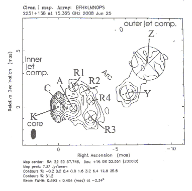
Figure 15: 15GHz-image of 3C454.3 measured on 25 June 2008. Knots R1,R2, R3 and R4 distribute along an arc-like structure in a fan area delimited by position angle=[–$45^{\circ}$, –$103^{\circ}$] and core separation $r_{n}$=[2 mas, 4 mas]. In comparion with the 43 GHz map (Fig.1 in the text), knot R3 could be associated with the jet-A in the double-nozzle scenario proposed for interpreting the 43 GHz kinematics. Thus the second radio burst observed at 15 GHz during 2005-2011 could originate from similar physical causes as the second burst observed at 43 GHz during 1999.8–2001.2.

In this paper we shall investigate the flux evolution observed at 43 GHz for two superluminal components in 3C454.3 (knot B4 and knot B6) and the connection with their kinematic properties. In order to search for the association of the flux variations with their Doppler-boosting effect, the model-fitting of their kinematic behaviors were performed more closely, taking into consideration of more details in the curves delineating their kinematics (e.g., the observed details in their core distance $r_{n}(t)$ and coordinate $Z_{n}(t)$ as function of time), which were ignored in the previous studies.
3C454.3 has a very complex structure at 43 GHz. A map observed at 2001.28 is shown in Figure 1 (cf. the sequence of maps presented in Fig.15 in Jorstad et al. Jo05 (2005)).

We shall utilize the results obtained for 3C454.3 by Qian et al. (Qi21 (2021)). In that work its thirteen superluminal components observed at 43 GHz were separated into two groups: group-A including the six components (B4, B5, K2, K3, K09 and K14) and group-B including the seven components (B1, B2, B3, B6, K1, K10 and K16).. Moreover, a double-jet structure (jet-A plus jet-B) was assumed to eject the superluminal knots of group-A and group-B, respectively. Interestingly, the kinematical behavior of the superluminal knots ascribed to group-A and group-B could be well model-fitted respectively in the framework of our precessing jet-nozzle scenario. It was found that both jets precess with the same precession period of 10.5 yr, but have different precessing common trajectory patterns.
As a supplement we shall discuss the flux evolution associated with the Doppler-boosting effect for the superluminal knot R3 observed at 15 GHz.

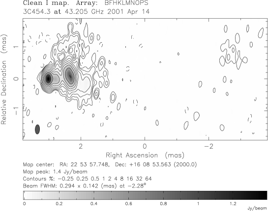
Figure 1: A 43 GHz image of 3C454.3 observed at 2001.28 (by courtesy of S.G.Jorstad, cf. Fig.44 in Jorstad et al. Jo05 (2005); also cf. Fig.15 (for a sequence of total intensity images during 1998.17–2001.28) and Fig.18 (for the trajectories of B4 and B6). On this map the positions of three knots (B4, B6 and D) should be indicated: knot B4 at position $[r_{n},PA]$=[1.16 mas, –$92.5^{\circ}$], knot B6 at position $[r_{n},PA]$=[0.70 mas, –$80.1^{\circ}$] and knot D at position $[r_{n},PA]$=[6 mas, –$82^{\circ}$]. The ejection position angles of B4 and B6 were $-80^{\circ}$ and $-150^{\circ}$ respectively. Their ejection epochs were 1998.36 and 1999.80. Thus a position angle swing of $\sim 70^{\circ}$ occurred in a short time-interval of $\sim$1.3 years. It seems that such a rapid swing could not be induced by a sudden ”jump” in the position angle of the jet-nozzle, but could be resulted from the two knots being ejected by two different nozzles. In the precessing jet-nozzle scenario for 3C454.3 (Qian et al. Qi21 (2021)), knot B4 and knot B6 are ascribed to jet-A and jet-B, respectively. In addition, there is an arc-like structure around the core which distributed in the area delimited by $r_{n}{\simeq}$[1.0–1.5 mas] and PA$\simeq$[–$30^{\circ}$, –$110^{\circ}$]. This arc-like structure is quite similar to that detected at 15 GHz by Britzen et al. (Br13 (2013)); cf. Fig.A.1 in the appendix.

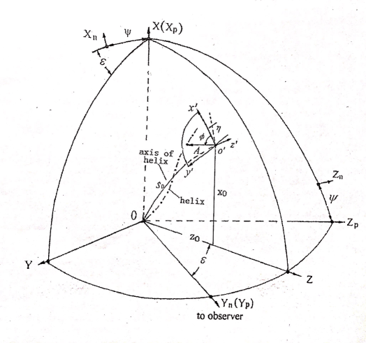
Figure 2: Geometry of the precessing nozzle scenario with a helical trajectory pattern.

2 Recapitulation of the precessing nozzle model: Geometry and formalism

In order to investigate the kinematic behavior and distribution of trajectory of the superluminal components on parsec scales in terms of our precessing jet-nozzle scenario, we define a special geometry in general case, where four coordinate systems are introduced (Qian et al. Qi21 (2021); Qian 2022a , 2022b ), as shown in Figure 2: (X,Y,Z), ($X_{n},Y_{n},Z_{n}$), ($X_{p},Y_{p},Z_{p}$), and (${\it{x}}^{\prime}$,${\it{y}}^{\prime}$,${\it{z}}^{\prime}$). Z-axis directs toward the observer, ($X_{n},Y_{n}$) and ($X_{p},Y_{p}$) define the plane of the sky with $X_{n}$-axis pointing toward the negative right ascension and $Z_{n}$-axis toward the north pole. Parameter $\epsilon$ defines the angle between Z-axis and $Y_{n}$-axis and $\psi$ the angle between X-axis and $X_{n}$-axis. Thus parameters $\epsilon$ and $\psi$ define the plane where the jet-axis ($x_{0}(z_{0})$) locates (see below). The helical trajectory of a knot can be described by the parameters A($s_{0}$) and $\phi(s_{0})$, which are defined in the coordinate system (${\it{x}}^{\prime}$,${\it{y}}^{\prime}$,${\it{z}}^{\prime}$) , where $s_{0}$ is the arc-length along the axis of the helix and ${\it{z}}^{\prime}$-axis is along the tangent of the axis of the helix. In addition, The helical trajectory precesses around the jet axis, producing the trajectories of different knots ejected at different times. That is superluminal components are ejected from the precessing jet nozzle at the helical phase $\phi$ which is related to the precession phase $\phi_{0}$. $\phi_{0}$ varies over a range of [0, 2$\pi$] during a precession period and is related to its ejection epoch $t_{0}$.
In the following we will adopt the formalism of the precessing nozzle scenario given in Qian et al. (Qi21 (2021)). The projection of the spatial trajectory of a knot on the sky-plane can be calculated by using the transformation between the coordinate systems. Superluminal knots are assumed to move on a helical trajectory defined by the parameters A($s_{0}$) (amplitude) and $\phi(s_{0})$ (phase), $s_{0}$ – arc-length along the jet axis which is defined by

$${x_{0}}(z_{0})=p(z_{0})({z_{0}}^{\zeta})$$ (1)

where

$$p({z_{0}})={p_{1}}+{p_{2}}[1+exp(\frac{{z_{t}}-{z_{0}}}{{z_{m}}})]^{-1}$$ (2)

$\zeta$, $p_{1}$, $p_{2}$, $z_{t}$ and $z_{m}$ are constants. $\zeta$=2 represents a parabolic shape for the axis of the helical trajectory.
The arc-length along the helical trajectory is $s_{0}$:

$${s_{0}}=\int_{0}^{z_{0}}{\sqrt{1+(\frac{d{x_{0}}}{d{z_{0}}})^{2}}}{d{z_{0}}}$$ (3)

The helical trajectory of a knot can be described in (X,Y,Z) system as follows.

$$X({s_{0}})=A({s_{0}}){\cos{\phi({s_{0}})}}{\cos{\eta({s_{0}})}}+{x_{0}}$$ (4)

$$Y({s_{0}})=A({s_{0}}){\sin{\phi({s_{0}})}}$$ (5)

$$Z({s_{0}})=A({s_{0}}){\cos{\phi({s_{0}})}}{\sin{\eta({s_{0}})}}+{z_{0}}$$ (6)

where $\tan{\eta({s_{0}})}$=$\frac{d{x_{0}}}{d{z_{0}}}$. The projection of the helical trajectory on the plane of the sky (or the apparent trajectory) is represented by

$${X_{n}}={X_{p}}{\cos{\psi}}-{Z_{p}}{\sin{\psi}}$$ (7)

$${Y_{n}}={X_{p}}{\sin{\psi}}+{Z_{p}}{\cos{\psi}}$$ (8)

where

$${X_{p}}={X({s_{0}})}$$ (9)

$${Z_{p}}={Z({s_{0}})}{\sin{\epsilon}}-{Y({s_{0}})}{\cos{\epsilon}}$$ (10)

All coordinates and amplitude (A) are measured in units of milliarcsecond. Introducing the following functions

$${\Delta}=\arctan[(\frac{dX}{dZ})^{2}+(\frac{dY}{dZ})^{2}]^{-\frac{1}{2}}$$ (11)

$${{\Delta}_{p}}=\arctan(\frac{dY}{dZ})$$ (12)

$${{\Delta}_{s}}=\arccos[(\frac{dX}{d{s_{0}}})^{2}+(\frac{dY}{d{s_{0}}})^{2}+(\frac{dZ}{d{s_{0}}})^{2}]^{-\frac{1}{2}}$$ (13)

We can then calculate the viewing angle $\theta$, apparent transverse velocity ${\beta}_{app}$, Doppler factor $\delta$ and the elapsed time T, at which the knot reaches distance $z_{0}$, as follows:

$${\theta}=\arccos[{\cos{\epsilon}}(\cos{\Delta}+\sin{\epsilon}\tan{{\Delta}_{p}})]$$ (14)

$${\delta}=[{\Gamma}(1-{\beta}{\cos{\theta}})]^{-1}$$ (15)

where $\Gamma$=$[1-{\beta}^{2}]^{-\frac{1}{2}}$ – bulk Lorentz factor, $\beta$=$\it{v}$/c, $\it{v}$ – velocity of the knot.

$${{\beta}_{app}}={{\beta}{\sin{\theta}}/(1-{\beta}{\cos{\theta}})}$$ (16)

$$T=\int^{{s_{0}}}_{0}{\frac{(1+z)}{{\Gamma\delta}{v}{\cos{{\Delta}_{s}}}}}{d{s_{0}}}$$ (17)

In this paper we shall adopt the concordant cosmological model (${\Lambda}CDM$) with $\Omega_{m}$=0.3, $\Omega_{\Lambda}$=0.7, and Hubble constant $H_{0}$=70km${s^{-1}}{Mpc^{-1}}$ (Spergel et al. Sp03 (2003)). Thus for 3C454.3, z=0.859, its luminosity distance is $D_{l}$=5.483 Gpc (Hogg Ho99 (1999), Pen Pe99 (1999)) and angular diameter distance $D_{a}$= 1.586 Gpc. Angular scale 1 mas=7.69 pc and proper motion of 1 mas/yr is equivalent to an apparent velocity of 46.48 c.

3 Knot B4: Model-fitting of kinematic behavior and 43 GHz light curve

As shown in the previous work (Qian et al. Qi21 (2021)) knot B4 was ejected from the nozzle associated with the jet-A in our precessing jet-nozzle scenario. Other knots attributed to jet-A are B5, K2, K3, K09 and K10. (Jorstad et al. Jo05 (2005), Jo10 (2010), Jo13 (2013)). The kinematic behavior of these knots has been consistently interpreted in terms of our scenario (Qian et al. Qi21 (2021)), but untill now their flux evolution has not been investigated.
Knot B4 produced two radio bursts. In order to investigate their flux evolution associated with its kinematic behavior we adopt the model parameters for jet-A as before:

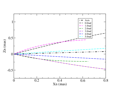
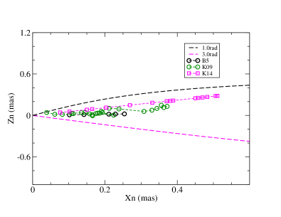
Figure 3: Jet-A. Left panel: the modeled distribution of the precessing common trajectories for the superluminal components at precessing phases $\phi$=0.0, 1.0,2.0, 3.0, 4.0 and 5.0, respectively. Right panel: the trajectories observed for knots B5, K09 and K14 within the jet-cone. The jet-axis is at position angle of $-84.3^{\circ}$.

(a) The plane, in which the jet axis locates, is defined by parameters $\epsilon$ and $\psi$: $\epsilon$=0.0126 rad=$0.72^{\circ}$, $\psi$=–0.1 rad=–$5.73^{\circ}$.
(b) The jet axis is defined by a set of parameters: $\zeta$=2, $p_{1}$=$p_{2}$=0, $z_{t}$=33 mas, $z_{m}$=3.0 mas (cf. equations 1 and 2).
(c) The precessing common trajectory pattern is assumed as: amplitude A=$A_{0}$$\sin(\pi{z_{0}}/{Z_{1}})$ with ($A_{0}$=0.727, $Z_{1}$=240 mas) and the helical phase $\phi$ identically equal to the precession phase $\phi_{0}$.
For jet-A the precession phase $\phi_{0}$ of the superluminal knots is related to the ejection epoch $t_{0}$ as follows:

$${\phi_{0}}(rad)=4.58+\frac{2\pi}{T_{0}}(t_{0}-1998.24)$$ (18)

In order to investigate the flux evolution associated with the Doppler boosting effect the observed flux density will be calculated as follows:

$${S_{obs}(\nu,t)}={S_{int}(\nu,t)}{\times}{[\delta(t)]^{3+\alpha(\nu,t)}}$$ (19)

where $S_{obs}$ – observed flux density, $S_{int}$ – intrinsic flux density ($S_{\nu}$ $\propto$ ${\nu}^{-\alpha}$) and $\alpha$ – spectral index.
The modeled distribution of the precessing trajectory for the superluminal components of jet-A is shown in Figure 3 (left panel) for precession phases $\phi$=0.0, 1.0, 2.0, 3.0, 4.0, 5.0 rad, respectively. The projected trajectories of B5, K09 and K14 within the jet-cone are shown in the right panel.
As shown in the previous paper (Qian et al. Qi21 (2021)), five superluminal components (B4, B5, K2, K3, K09 and K14) of jet-A were found to undergo accelerated/decelerated motion, revealing increase/decrease in their bulk Lorentz factor and Doppler factor. However, their flux evolution due to the Doppler-boosting effect has not been investigated. Here we shall model-fit the 43 GHz light curve for knot B4 in terms of its Doppler-boosting effect in combination with the explanation of its kinematics.

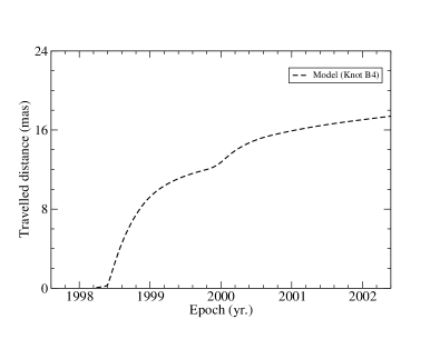
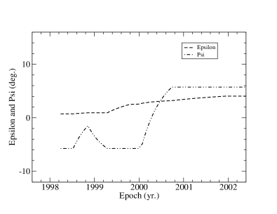
Figure 4: Knot B4: the modeled traveled distance Z(t) along the jet axis (left panel) and the modeled curves for the parameter $\epsilon(t)$ and $\psi(t)$ defining the plane where the jet-axis locates. Before 1998.52 $\epsilon$=$0.72^{\circ}$ and $\psi$=–$5.73^{\circ}$, B4 moved along the precessing common trajectory. After 1998.52 B4 started to move along it own individual track. During the two radio bursts ($\sim$1998.4–1999.4 and $\sim$1999.9–2001.2) parameter $\psi$ varied quite largely.

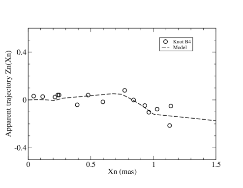
Figure 5: Knot B4: the model-fit of the observed trajectory $Z_{n}(X_{n})$. Within $\sim$0.07 mas of the coordinate $X_{n}$ B4 moved along the precessing common trajectory, while beyond that it moved along its own individual track, deviating from the common track. A prominent curvature occurred at $r_{n}\simeq$0.7–1.2 mas.

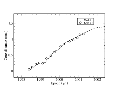
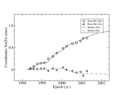
Figure 6: Knot B4: the model-fits of the core separation $r_{n}(t)$ and coordinates $X_{n}(t)$ and $Z_{n}(t)$. These fits are almost perfect (especially the fit for $Z_{n}(t)$) and much better than those previously presented in Qian et al. (Qi21 (2021)) due to carefully having taken the details in its kinematic behavior into full account (especially details in $r_{n}(t)$, d$r_{n}$/dt and $Z_{n}(t)$).

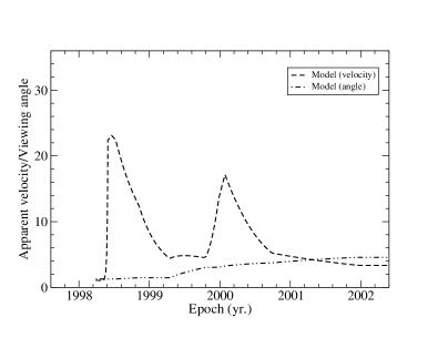
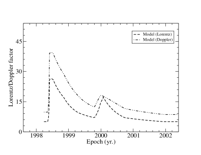
Figure 7: Knot B4. Left panel: the model-derived apparent velocity $\beta_{app}(t)$ and viewing angle $\theta(t)$. Right panel: the model-derived bulk Lorentz factor $\Gamma(t)$ and Doppler factor $\delta(t)$. $\Gamma(t)$, $\delta(t)$ and $\beta_{app}(t)$ all show a double-peak structure closely related to its two radio bursts. At the first peak (epoch 1998.5) $\delta_{max}$=39.5, $\Gamma_{max}$=26.5, $\beta_{app,max}$=23.1 and $\theta$=$1.26^{\circ}$, while at the second peak (epoch 2000.0) $\delta$=$\delta_{max}$=18.0, $\Gamma$=14.9, $\beta_{app}$=14.5 and $\theta$=$3.1^{\circ}$. The maximum Lorentz factor was not coincident with the maximum Doppler factor: at 2000.1 $\Gamma$=$\Gamma_{max}$=17.2, $\delta$=17.7, $\beta$=$\beta_{app,max}$=17.1 and $\theta$=$3.24^{\circ}$. Our model-fitting results for the apparent velocity are quite different from those given in Jorstad et al. (Jo05 (2005); cf. its Fig.30) which were determined by using polynominal approximations. Figs.5–7 demonstrate that the entire kinematics observed within core separation ${r_{n}}{\simeq}$1.2 mas (corresponding to the traveled distance Z=16.3 mas$\simeq$125 pc) can be well explained in terms of our precessing nozzle scenario.

3.1 Knot B4: model-fitting results of kinematics

The model-fitting results of its kinematics are shown in Figures 4-7.
The traveled distance Z(t) along the jet-axis (left panel) and the modeled curves for parameters $\epsilon(t)$ and $\psi(t)$ are shown in Fig.4. Before 1998.52, or core distance $r_{n}{\leq}$0.066 mas (Z$\leq$23.0 pc), $\epsilon$=$0.72^{\circ}$ and $\psi$=–$5.73^{\circ}$, knot B4 moved along the precessing common trajectory, while after 1998.52 it started to move along its own individual trajectory, where parameter $\psi$ showed quite large changes during the two radio bursts in (1998.4–1999.4) and (1999.9–2001.2).
In the model fitting its precession phase was assumed to be $\phi_{0}$=4.58 rad and the corresponding ejection time $t_{0}$=1998.24, well consistent with the ejection time 1998.36$\pm$0.07 derived by Jorstad et al. (Jo05 (2005)).
It can be seen from Figs. 5 and 6 that its entire kinematic features (including trajectory $Z_{n}(X_{n})$, core separation $r_{n}(t)$, coordinates $X_{n}(t)$ and $Z_{n}(t)$) are all well fitted extending to core separation $r_{n}{\sim}$1.2 mas. The model-derived apparent velocity $\beta_{app}(t)$, viewing angle $\theta(t)$, bulk Lorentz factor $\Gamma(t)$ and Doppler factor $\delta(t)$ are shown in Fig.7. $\Gamma(t)$, $\delta(t)$ and $\beta_{app}(t)$ all have a double-peak structure, corresponding to the double-peak structure of the light curve (Fig.8). The viewing angle $\theta(t)$ varied from ${\sim}1.3^{\circ}$ (1998.3) to ${\sim}4.6^{\circ}$ (2002.0).

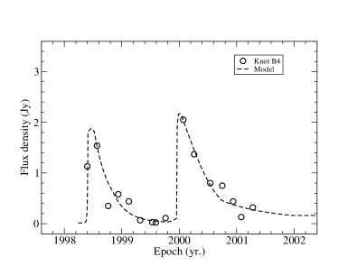
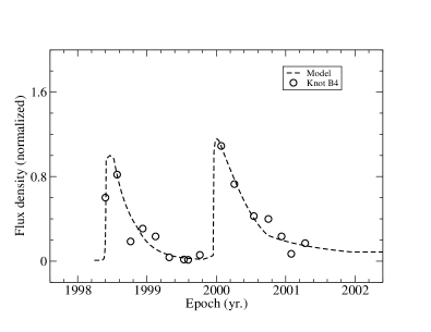
Figure 8: Knot B4. Left panel: the model fit of the 43 GHz light curve. The modeled peak flux densities are 1.88 Jy (at 1998.5) and 2.17 Jy (at 2000.0), respectively. The intrinsic flux density of the first burst was 4.86$\mu$Jy. Right panel: the light curve normalized by the modeled peak flux density of the first burst is well fitted by the Doppler boosting profile $[\delta(t)/\delta_{max}]^{3+\alpha}$ ($\alpha$ was asssumed to be 0.5). The second burst had its Doppler factor ($\delta_{max}$=18.0) much smaller than the first burst ($\delta_{max}$=39.5), while its observed flux density (2.17 Jy) was larger than that (1.88 Jy) of the first burst. Thus in the model fitting of the flux evolution the intrinsic flux density of the second burst was assumed to be eighteen times that of the first burst (i.e., 87.5$\mu$Jy for the second burst).

3.2 Knot B4: Flux evolution and Doppler-boosting effect

B4 produced two radio bursts during 1998.4–1999.4 and 1999.9–2001.2. In order to interpret the entire lightcurve, the model parameters ($\epsilon(t)$, $\psi(t)$ and $\Gamma(t)$) were carefully and consistently selected and we paid much more attention on the details in the observed kinematic behavior (especially on the details in $r_{n}(t)$, $dr_{n}/dt$ and $Z_{n}(t)$).
The model-fit results of the entire light curve (including both the radio bursts) are shown in Figure 8. For the first burst, the epoch of the modeled peak $t_{max}$=1998.47 with the maximum Doppler factor $\delta_{max}$=39.49 and the maximum flux density $S_{max}$=1.88 Jy, while its intrinsic flux density $S_{int}$=4.86 $\mu$Jy.
For the second burst, the epoch of the modeled peak $t_{max}$=2000.01 with the maximum Doppler factor $\delta_{max}$=18.02 and maximum flux density $S_{max}$=2.17 Jy, while its intrinsic flux density $S_{int}$=87.5 $\mu$Jy. It should be noted that the second burst originated from its re-acceleration in the convergence/collimation region near the position [$r_{n}$=0.6–1.2 mas, PA=$\sim$${-90^{\circ}}$], where parameter $\psi$ rapidly increased, resulting in the southwest curvature of its trajectory (Figs. 4–6).

4 Knot B6: Model fitting of kinematic behavior and 43 GHz light curve

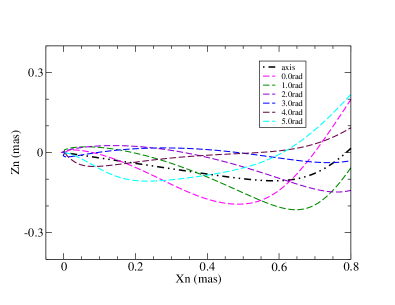
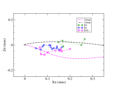
Figure 9: Jet-B. Left panel: the modeled distribution of the precessing common trajectories for the superluminal components at precession phases $\phi$=0.0, 1.0, 2.0, 3.0, 4.0 and 5.0 rad, repectively. Right panel: the projected trajectories of knots B3, K1 and K10 within the jet cone. The jet-axis is at position angle –$101.5^{\circ}$.

As in the previous work superluminal knots B6 and B1, B2, B3, K1, K10, K16 were assumed to be ejected by the nozzle of jet-B. For jet-B the modeled distribution of the precessing common trajectories for its superluminal components is shown in Fig.9. We shall use the same model parameters as before (Qian et al. Qi21 (2021)).
(a) The jet-axis locates in a plane defined by the parameters $\epsilon$=0.0126 rad=$0.72^{\circ}$ and $\psi$=0.20 rad=$11.46^{\circ}$.
(b) The shape of the jet-axis is defined by a set of parameters: $\zeta$=2, $p_{1}$=0, $p_{2}$=1.34$\times$$10^{-4}$/mas, $z_{t}$=66 mas and $z_{m}$=6.0 mas (cf. equations 1 and 2).
(c) The common precessing trajectory pattern is defined by the amplitude parameter A=${A_{0}}{[\sin(\pi{z_{0}}/{Z_{1}})]^{1/2}}$ with ($A_{0}$=0.182 mas and $Z_{1}$=396 mas) and helical phase $\phi$=$\phi_{0}$–$(z_{0}/Z_{2})^{1/2}$ with $Z_{2}$=3.58 mas and $\phi_{0}$ being the precession phase which is related to its ejection time $t_{0}$ as follows:

$${\phi_{0}}(rad)=0.42+\frac{2\pi}{T_{0}}(t_{0}-1994.46)$$ (20)

As shown in the previous paper (Qian et al. Qi21 (2021)), four superluminal components (B2, B6, K1 and K16) of jet-B were found to participate in accelerated/decelerated motions, showing the trends of increasing/decreasing in their bulk Lorentz factor and Doppler factor. However, untill now their flux evolution due to the Doppler-boosting effect has not been investigated. Here we shall model-fit the 43 GHz light curve for knot B6 in combination with the explanation of its kinematics.

5 Knot B6: model-fitting results of kinematics

The model fitting results of its kinematics are shown in Figures 10–13.
Its ejection time $t_{0}$=1999.61, well consistent with that ($t_{0}$=1999.80$\pm$0.37) given by Jorstad et al. (Jo05 (2005)) and the corresponding precession phase $\phi_{0}$=3.50 rad.
The modeled traveled distance Z(t) along the jet-axis and the model-derived curves for the parameters $\epsilon(t)$ and $\psi(t)$ are shown in Fig.10. Before 2000.54 (or $r_{n}{\leq}$0.18 mas) $\epsilon$=$0.72^{\circ}$ and $\psi$=$11.5^{\circ}$, knot B6 moved along the precessing common trajectory. After 2000.54 $\psi$ quickly decreased to $-4.6^{\circ}$ and B6 started to move along its own individual track, deviating from the precessing common trajectory.
The model-fitting results of the observed trajectory $Z_{n}(X_{n})$, distance from the core $r_{n}(t)$, coordinates $X_{n}(t)$ and $Z_{n}(t)$ are shown in Figs. 11 and 12. All these kinematic features were well fitted by the precessing nozzle scenario.
The model-derived curves for Lorentz factor $\Gamma(t)$, Doppler factor $\delta(t)$, apparent velocity $\beta_{app}(t)$ and viewing angle $\theta(t)$ are shwon in Fig.13. $\Gamma(t)$, $\delta(t)$ and $\beta_{app}(t)$ all have a bump structure. At 2000.30 $\Gamma_{max}$=30.5, and $\delta_{max}$=56.0, but $\beta_{app,max}$=21.4 at 2000.6. The viewing angle $\theta(t)$ varied in the range [$0.72^{\circ}$(1999.6)–$0.38^{\circ}$(2000.0)–$1.63^{\circ}$(2001.5)].

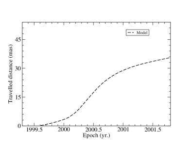
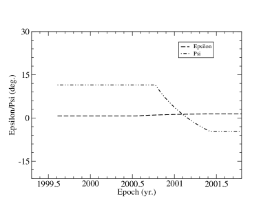
Figure 10: Knot B6: the modeled traveled distance Z(t) along the jet axis (left panel) and the model-derived curves for the parameters $\epsilon(t)$ and $\psi(t)$ which define the plane where the axis of jet-B locates. Before 2000.54 (or $r_{n}{\leq}$0.18 mas, corresponding to Z$\leq$19.0 mas=146 pc) $\epsilon$=$0.72^{\circ}$ and $\psi$=$11.5^{\circ}$, knot B6 moved along the precessing common track. After 2000.54 $\psi$ rapidly decreased to –$4.6^{\circ}$ (at 2001.4, knot B6 started to move along its own individual trajectory, deviating from the precessing common track.

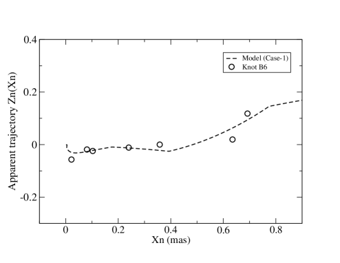
Figure 11: Knot B6: the model fit of the apparent trajectory. Within core separation $r_{n}{\sim}$0.18 mas (or before 2000.54, corresponding to the traveled distance Z$\leq$19.0 mas=146 pc) $\epsilon$=$0.72^{\circ}$ and $\psi$=$11.5^{\circ}$, knot B6 moved along the precessing common trajectory with its precession phase $\phi_{0}$=3.50 rad. Beyond $r_{n}$=0.18 mas it started to move along its own individual track, deviating from the precessing common trajectory.

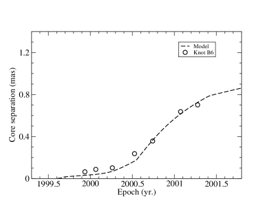
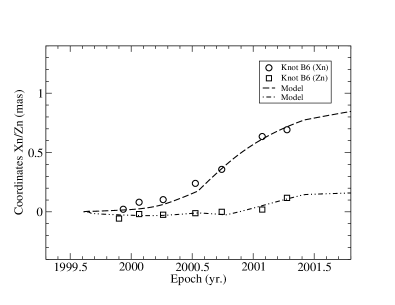
Figure 12: Knot B6: the model-fits of the core separation $r_{n}(t)$ (left panel) and the coordinates $X_{n}(t)$ and $Z_{n}(t)$ (right panel). All these kinematic features are well fitted by the precessing nozzle scenario. The radio burst occurred during $\sim$2000–2001 is associated with its accelerated/decelerated motion.

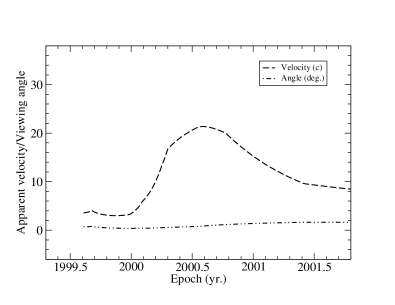
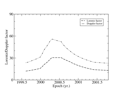
Figure 13: Knot B6: the model-derived apparent velocity $\beta_{app}$ and viewing angle $\theta(t)$ (left panel), and the model-derived bulk Lorentz factor $\Gamma(t)$ and Doppler factor $\delta(t)$ (right panel). $\beta_{app}$, $\Gamma$ and $\delta$ all have a bump structure. At 2000.30 $\delta$=$\delta_{max}$=55.9 and $\Gamma$=$\Gamma_{max}$=30.5, while $\beta$=$\beta_{max}$=21.4 at 2000.59; $\theta(t)$ varied in the range [$0.72^{\circ}$ (1999.6), $0.38^{\circ}$ (2000.0), $1.63^{\circ}$ (2001.5)]

.

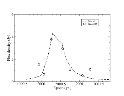
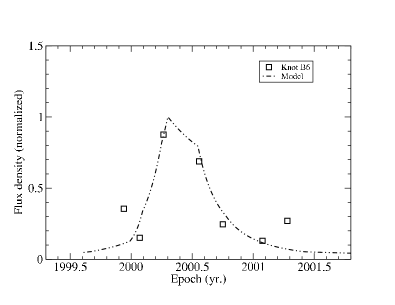
Figure 14: Knot B6: the model-fit of its light curve. The 43 GHz light curve is well fitted by the Doppler-boosting effect with the modeled peak flux density of 4.31 Jy at 2000.3 and its intrinsic flux density 3.3$\mu$Jy (left panel). The light curve normalized by the modeled peak flux is well fitted by its Doppler-boosting profile $[\delta/\delta_{max}]^{3+\alpha}$ with an assumed value of $\alpha$=0.5.

5.1 Knot B6: Flux evolution and Doppler-boosting effect

As for the case of knot B4 we calculated the observed light curve by using equation (19) in order to take account of its Doppler boosting effect. The model fit of its light curve is shown in Figure 14. It can be seen that the 43 GHz light curve is well fitted with the modeled peak flux density 4.31 Jy at 2000.30 and an intrinsic flux density of 3.3$\mu$ Jy (left panel). The light curve normalized by the modeled peak flux density is well fitted by its Doppler-boosting profile $[\delta(t)/\delta_{max}]^{3+\alpha}$ with a presumed value of $\alpha$=0.5 (right panel).

6 Knot R3: model fitting results of kinematics and light curve observed at 15 GHz

Two characteristics should be emphasized: (1) An arc-like structure was detected at 15 GHz; (2) Its light curve comprises two radio bursts. These features are very similar to those of knot B4 observed at 43 GHz. See Appendix.

7 Discussion and Conclusion

We have applied the precessing jet-nozzle scenario proposed previously (e.g. Qian et al. Qi91 (1991), Qi14 (2014), Qi21 (2021); Qian 2022a , 2022b ) to successfully model-fit the kinematic behavior of the superluminal components B4 and B6 in blazar 3C454.3 and nicely explain the 43 GHz light curves in terms of their Doppler-boosting effect. Thus their kinematic properties (including the entire trajectory $Z_{n}(X_{n})$, core separation $r_{n}(t)$ and coordinates $X_{n}(t)$ and $Z_{n}(t)$) and their flux evolution have been completely interpreted as a whole. Their kinemtic parameters (including bulk Lorentz factor $\Gamma(t)$, Doppler factor $\delta(t)$, viewing angle $\theta(t)$ and apparent velocity $\beta_{app}(t)$ as function of time) have been correctly determined.
In order to achieve this goal, we have carefully taken some significant details in their kinematic behavior (e.g., details in the observed core-separation curve ${r_{n}(t)}$ and in the coordinate $Z_{n}(t)$) into full account, which were neglected in the previous work (Qian et al. Qi21 (2021)).
Obviously, similar studies can also be done for more components (e.g., B5, K3, K09, K14 (jet-A) and B2, K1, K16 (jet-B)) to associate their flux evolution with their Doppler boosting effect, because the modeled curves of Lorentz/Doppler factor for these components were already derived approximately in Qian et al. (Qi21 (2021)). It seems that the optical light curves of superluminal knots observed in 3C454.3 (Jorstad et al. Jo10 (2010), Jo13 (2013)) could also be studied within the framework of our precessing nozzle scenario, if the precessing common trajectory patterns (e.g., helical patterns on much smaller scales) are correctly selected (cf. Qian 2018b ).
The full explanation of the kinematics and flux evolution observed at 43 GHz for both B4 and B6 in terms of the precessing nozzle sceanrio has further clarified the distinct features in 3C454.3: (1) its superluminal components could be separated into two groups which have different kinematic and flaring properties. For example, knot B4 moved southwest along a curved trajectory extending to core separation of $\sim$1.2 mas, passing through a convergence/recollimation region and producing a major burst. Moreover, the track of knot B4 could be connected to that of knot D at core distance $\sim$6 mas (cf. Fig.1). In contrast, knot B6 moved northwest along a track only extending to core distance of $\sim$0.7 mas without any flaring activity in the outer jet region. The VLBI observations at 15 GHz also revealed that knot R3 had its kinematic behavior similar to that of knot B4 observed at 43 GHz, while the kinematic behavior of knot R1 and R2 was quite different from that of knot R3; (2) At both 43 GHz and 15 GHz a prominent arc-like structure was detected, distributing over a very broad range of position angle from $\sim$–${120^{\circ}}$ to $\sim$–${30^{\circ}}$. A rapid position angle swing of $\sim$${70^{\circ}}$ between knot B4 and knot B6 in $\sim$1.3 years might be regarded as a clue for the existence of a double-jet structure in 3C454.3, indicating that knot B4 and knot B6 were ejected from their respective jet; (3) The recurrent trajectory patterns found in the knot-pairs B4/K09, B6/K10 and B2/K14 may be regarded as favorable evidence to suggest some periodic behavior in knots’ kinematics induced by the jet-nozzle precession with a precession period of $\sim$10.5 yr and the possible existence of a precessing common trajectory. Such kind of periodic recurrence of curved trajectory patterns seems to be important signatures for recognizing nozzle precession and determining precession periods for blazars; (4) Knot B4 produced two radio bursts at 43 GHz: one occurred near the core and the other in the outer jet region. Similarly, knot R3 also produced two radio bursts at 15 GHz, but at different core distances. Both the bursts can be interpreted in terms of Doppler-boosting effect. This similarity observed at diffrent frequencies might indicate the stability of the track patterns for knot B4 and knot R3.
Our precessing nozzle scenario is based on the two assumptions: (1) Superluminal components are ejected from a jet-nozzle at corresponding precession phases when the jet-nozzle precesses. Here for 3C454.3, the precession period is found to be 10.5 years; (2) Superluminal components move along their common precessing tracks in the innermost jet regions with a transition at certain core-distances in the outer-jet regions from precessing common tracks to their own individual trajectories.
However, these assumptions may imply to introduce severe constraints on the precessing nozzle secnario when it is applied to investigate the VLBI-kinematics of superluminal components in blazar 3C454.3 (Qian et al. Qi21 (2021)). That is, these assumptions may be ”unavoidable” to require double precessing-nozzle structures existing in these blazars. Otherwise, if ”single jet-nozzle” structures are assumed for these blazars, there would be no unified nozzle-precession to be explored for consistently delineating the kinematics of their superluminal components as a whole. One would have to deal with the kinematics of many superluminal components which are independent of each other. Thus it would be difficult to clarify their respective characteristics and connections to the central engine (the black hole/accretion disk system in its nucleus) for the components as a whole.
In contrast, for quasars (e.g., B1308+328, PG1302-102 and NRAO 150) the precessing jet-nozzle scenario with a single jet structure may be applicable to determine their precession periods (Qian et al. 2018a , Qi17 (2017); Qian Qi16 (2016) and Qian Qi23 (2023)).
Therefore, at present, the assumption of ”double jet-nozzle structure” for blazar 3C454.3 (also for blazars 3C279, 3C345 and OJ287) may be regarded as a ”working hypothesis”, although it has initiated some physically meaningful results and there are some observational clues in favor of this suggestion.
In summary, we have applied our precessing nozzle scenario to study the kinematics and flux evolution of superluminal components in a few QSOs and blazars, determining their precession periods and precessing common trajectory patterns. For quasars B1308+326, PG1302-102 and NRAO150 only single jet structure has been assumed, while for blazars 3C279, 3C345, 3C454.3 and OJ287 double-jet structures are assumed. In all these cases the flux evolution of superluminal components can be interpreted in terms of their Doppler-boosting effect, although their intrinsic variations on shorter time-scales induced by the evolution of superluminal knots (superluminal plasmoids or relativistic shocks) need to be taken into account. The combined effects of Doppler-boosting and intrinsic variation in the flux evolution of superluminal components have also been found in blazar 3C345 (especially for its knots C9 and C10; Qian 2022a , 2022b ).
Generally, the assumption of precessing common trajectory may be applicable, but the model-derived patterns and their extensions are quite different for different superluminal knots (Qian et al. Qi21 (2021) and references therein). Higher resolution VLBI observations are needed to show if this assumption is still valid within core separations $<$0.1 mas.
Theoretically, this assumption may be based on the theoretical works of relativistic magnetohydrodynamics for jet formation: magnetic effects in acceleration/collimation zone of relativistic jets are very strong, forming some very solid magnetic structures and controlling the trajectory patterns of moving superluminal knots ejected from the jet nozzle (e.g., Vlahakis & Königl Vl04 (2004), Blandford & Payne Bl82 (1982), Blandford & Znajek Bl77 (1977), Camenzind Cam90 (1990) and references therein). Thus all the superluminal components in a blazar can move along the precessing common trajectory if the jet nozzle is precessing.

Appendix A Flux evolution of superluminal knot R3 observed at 15GHz

3C454.3 has a very complex structure at 15 GHz as like at 43 GHz. The most distinctive and prominent feature found by the VLBI-observations at 15 GHz during the period (1995 Jul.29–2010 Nov.20; Britzen et al. Br13 (2013), Qian et al. Qi14 (2014)) was the evolving arc-like structure around the core (Figs.A.1 and A.2), which was constituted by the knots (R1, R2, R4 and R3) moving along different curved trajectories and distributing in an area delimited by $r_{n}{\simeq}$[2.5, 3.5] mas and PA${\simeq}$[–$40^{\circ}$, –$110^{\circ}$]. Such an arc-like structure observed at 15 GHz is evry similar to that observed at 43 GHz (cf. Fig.1 in the text), but at different distances to the core.
The kinematic behavior of its eight superluminal components (R1, R2, R3, R4, A, B, C and D) has been analyzed (Qian et al. Qi14 (2014)). It was found that their kinematic features (including the projected trajectory and the core separation and coordinates versus time) could be well model-fitted and interpreted in terms of our precessing jet-nozzle scenario. Their apparent velocity/viewing angle and bulk-Lorentz/Doppler factor as function of time were derived.
In addition, knot R3 was tracked by the 15 GHz VLBI observations from core distance ${r_{n}}\sim$0.7 mas to $\sim$3.7 mas and a prominent trajectory-curvature at core distances $\sim$2–3.84 mas (Figs.A.4. and A.5) was detected. Interestingly, a radio flare was observed during $\sim$2005–2012 to be closely associated with this curvature (Fig.A.7). This phenomenon could be related to the convergence and re-collimation of the ’mini-jet (or beam)’ associated with the knot (R3), resulting in its re-acceleration and an increase in its bulk Lorentz factor (cf. Figs. A.2–A.6).
It should be noted that knot R3 produced two flares at 15 GHz: one in $\sim$1995 (only part of it was measured) and the other during $\sim$2005–2012. So the flaring behavior of knot R3 at 15 GHz is quite similar to the flaring behavior of knot B4 at 43 GHz, which also produced two flares with the second one associated with the trajectory-curvature at $r_{n}{\simeq}$0.7–1.2 mas (during $\sim$1999.8–2001.4; cf. Figs. 5–8 in the text).

A.1 Knot R3: model-fitting of kinematics at 15 GHz

The kinematics observed at 15 GHz for knot R3 has already been well model-fitted in terms of our precessing jet-nozzle scenario in Qian et al. (Qi14 (2014)), where the precessing common trajectory pattern and its ejection epoch ($t_{0}$=1992.0 corresponding to a precession phase $\phi$=5.75 rad) were determined. We shall utilize these results and more carefully perform the model-fits of its kinematic features (trajectory $Z_{n}(X_{n})$, core distance $r_{n}(t)$, coordinates $X_{n}(t)$ and $Z_{n}(t)$) in order to correctly derive its bulk Lorentz factor $\Gamma(t)$ and Doppler factor $\delta(t)$ for explaining its flux-density evolution.

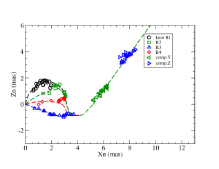
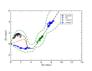
Figure 16: A conceptual sketch illustrating the apparent convergence of the jet-trajectories and the formation of the arc-like structure (Qian et al. Qi14 (2014)). Near the position ($X_{n}$, $Z_{n}$)=(3.0 mas, –1.0 mas) knot R3 passed through a convergence/recollimation region and then it moved toward the direction of knot Y, producing a radio burst. In contrast, knots R1 and R2 had no extensions along the position angles of $\sim$–$40^{\circ}$ – $\sim$–$50^{\circ}$. The green dashed lines in the right panel indicate the jet boundaries defined by the sizes of the superluminal components.

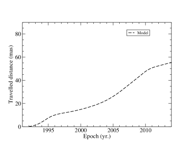
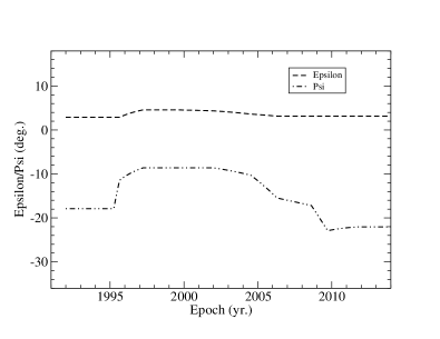
Figure 17: Knot R3: the model-simulated traveled distance $Z(t)$ along the Z-axis (left panel) and the modeled curves of parameters $\epsilon(t)$ and $\psi(t)$, which define the plane where the jet-axis locates. In the innermost jet region (core separation $r_{n}{\leq}$0.58 mas (or before 1995.25) knot R3 moved along the precessing common trajectory with its precession phase $\phi$=5.75 rad and corresponding ejection time $t_{0}$=1992.0. After 1995.25 $\psi$ changed largely and R3 started to move along its own individual track. During 2005–2011 parameter $\psi$ decreased quickly, inducing an oscillating curvature in its trajectory (Fig.A.4).

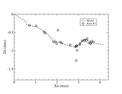
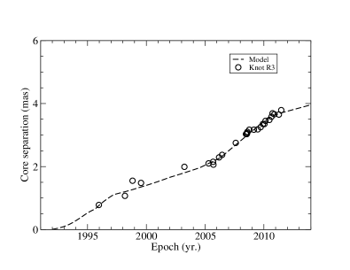
Figure 18: Knot R3: the model-fits of the projected trajectory $Z_{n}(X_{n})$ (left panel) and the core separation $r_{n}(t)$. The entire trajectory extending to $r_{n}{\sim}$3.8 mas (Z=408.3 pc) was well fitted, especially the oscillating curvature in the range of $X_{n}{\sim}$[2–3.8] mas. Within $X_{n}{\sim}$0.54 mas (Z$\leq$8.3 mas=63.8 pc; or before $\sim$1995.25) knot R3 moved along the precessing common trajectory. Unfortunately no VLBI-observations were performed then. After 1995.25 knot R3 started to move along its own individual track, deviating from the precessing common trajectory.

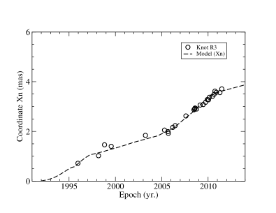
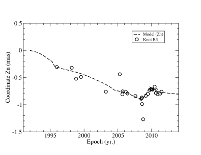
Figure 19: Knot R3: the model-fits of the coordinates $X_{n}(t)$ and $Z_{n}(t)$ which were well fitted entirely, especially the oscillating curvature during 2005–2011 (right panel).

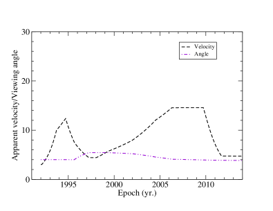
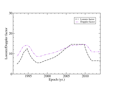
Figure 20: Knot R3: the model-derived apparent velocity $\beta_{app}(t)$ and viewing angle $\theta(t)$ (left panel) and the model-derived bulk Lorentz factor $\Gamma(t)$ and Doppler factor $\delta(t)$. $\beta_{app}(t)$, $\Gamma(t)$ and $\delta(t)$ all have a double-bump structure: at the first peak (epoch 1994.70): $\delta_{max}$=14.2, $\Gamma_{max}$=12.5 and $\beta_{app,max}$=12.3. At the second peak (epoch 2009.80), $\delta_{max}$=14.6, $\beta_{app}$=14.1 and $\Gamma$=14.2, while at 2009.73 $\Gamma_{max}$=14.6, $\beta_{app,max}$=14.6 and $\delta$=14.5. The viewing angle $\theta(t)$ varied in the range [$3.9^{\circ}$(1992.0)–$5.4^{\circ}$(1997.2)–$3.9^{\circ}$(2011.0)].

The model-fitting results are presented in Figs. A.3–A.7. In Fig.A.3 are presented the traveled distance Z(t) along the jet-axis (left panel) and the model-derived curves for parameters $\epsilon(t)$ and $\psi(t)$ (right panel). Within core separation $r_{n}$=0.58 mas (corresponding to Z$\leq$8.3 mas=63.8 pc, or before 1995.25), [$\epsilon$, $\psi$]=[$2.88^{\circ}$, –$17.9^{\circ}$], knot R3 moved along the precessing common trajectory with its precession phase $\phi$=5.75 rad and ejection time $t_{0}$=1992.0. After 1995.25 parameter $\psi$ changed largely and R3 started to move along its own individual track, deviating from the precessing common trajectory. During the time-interval $\sim$2005–2011 ($X_{n}{\simeq}$2–3.8 mas) changes in parameter $\psi$ resulted in an oscillating curvature in its trajectory (Fig. A.4, left panel).

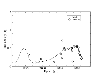
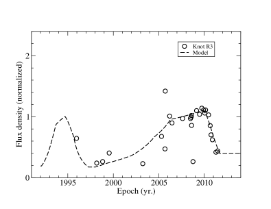
Figure 21: Knot R3. Left panel: the model-fit of the 15 GHz light curve in terms of the Doppler-boosting effect with the peak flux density being 0.50 Jy and 0.55 Jy for the two radio bursts, respectively. The intrinsic flux density $S_{int}$=46.6$\mu$Jy. Right panel: the model-fit of the light curve normalized by the peak flux density of the first burst was well fitted in terms of the Doppler-boosting profile $[\delta(t)/\delta_{max}]^{3+\alpha}$ with an assumed value for $\alpha$=0.5.

The model-fits of the trajectory $Z_{n}(X_{n})$, core separarion $r_{n}(t)$, coordinates $X_{n}(t)$ and $Z_{n}(t)$ are shown in Figs. A.4 and A.5, respectively. It can be seen that all the kinematic features were precisely fitted with the entire trajectory extending to core separation of $\sim$3.8 mas and the oscillating curvature in the trajectory at $X_{n}{\simeq}$2–3.8 mas.
The model-derived apparent velocity $\beta_{app}(t)$ and viewing angle $\theta(t)$ are presented in Fig.A.6 (left panel). The model-derived bulk Lorentz factor $\Gamma(t)$ and Doppler factor $\delta(t)$ are shown in Fig.A.6 (right panel). The model-derived curves for $\beta_{app}(t)$, $\Gamma(t)$ and $\delta(t)$ all have two-bump structures corresponding to the two radio bursts. At the first bump (epoch 1994.7): $\delta_{max}$=14.2, $\Gamma$=$\Gamma_{max}$=12.5 and $\beta_{app}$=$\beta_{app,max}$=12.3. For the second broad bump, at epoch 2009.80: $\delta_{max}$=14.6, $\Gamma$=14.2 and $\beta_{app}$=12.1, while at epoch 2009.73 $\Gamma$=$\Gamma_{max}$=14.6, $\beta_{app}$=$\beta_{app,max}$=14.6 and $\delta$=14.54. The viewing angle $\theta(t)$ varied in the range of [$3.9^{\circ}$(1992.0)–$5.4^{\circ}$(1997.2)–$3.9^{\circ}$(2011.0)].

A.2 Knot R3: model-fit of 15 GHz light curve

Since the kinematics of knot R3 was successfully model-fitted and its bulk Lorentz factor and Doppler factor versus time were precisely derived, the 15 GHz light curve of knot R3 was well fitted in terms of its Doppler boosting effect, as shown in Fig.A.7. The model-fit of the observed light curve is shown in the left panel with its peak flux density 0.50 Jy and intrinsic flux density of 46.6$\mu$Jy. The light curve normalized by the peak flux density of the first burst was well fitted by the Doppler-boosting profile $[\delta(t)/\delta_{max}]^{3+\alpha}$ with a presumed value $\alpha$=0.5 as shown in the right panel. The peak flux density of the second burst is modeled as 0.55 Jy.
It worths noting that the second burst (during $\sim$2005–2010) of knot R3 occurred in the outer jet-regions at core distances $r_{n}{\simeq}$[2.0–3.8] mas, where its trajectory underwent an oscillating curvature (Fig.A.4). This curvature was induced by the change in the parameter $\psi$ (Fig.A.3), which did not affect the variations in the flux-density of knot R3. The second radio burst is mainly induced by the Doppler boosting effect due to the increase/decrease in its bulk Lorentz factor and Doppler factor (Fig.A.6, right panel).
The similarity of the morphological structures observed at 15 GHz and 43 GHz for 3C454.3, and the occurrence of the second radio burst observed in knot R3 (at 15GHz) and B4 (at 43GHz) clearly demonstrate that some similar physical environments, kinematic structures and conditions may exist on different scales in 3C454.3, resulting in similar kinematic and emission properties for the superluminal components observed at different frequencies, although they moved along different tracks with different speeds.