Saltation Matrices:
The Essential Tool for Linearizing Hybrid Dynamical Systems

Abstract

Hybrid dynamical systems, i.e. systems that have both continuous and discrete states, are ubiquitous in engineering, but are difficult to work with due to their discontinuous transitions. For example, a robot leg is able to exert very little control effort while it is in the air compared to when it is on the ground. When the leg hits the ground, the penetrating velocity instantaneously collapses to zero. These instantaneous changes in dynamics and discontinuities (or jumps) in state make standard smooth tools for planning, estimation, control, and learning difficult for hybrid systems. One of the key tools for accounting for these jumps is called the saltation matrix. The saltation matrix is the sensitivity update when a hybrid jump occurs and has been used in a variety of fields including robotics, power circuits, and computational neuroscience. This paper presents an intuitive derivation of the saltation matrix and discusses what it captures, where it has been used in the past, how it is used for linear and quadratic forms, how it is computed for rigid body systems with unilateral constraints, and some of the structural properties of the saltation matrix in these cases.

I Introduction

Many interesting problems in engineering can be modeled as hybrid dynamical systems, meaning that they involve both continuous and discrete evolution in state [1, 2, 3, 4]. These systems can be hybrid, e.g. due to physical contact, a result of digital logic circuits, or they can be triggered by control – reacting to sensor feedback or switching control modes. Meanwhile, most of the tools that exist for planning, estimation, control, and learning assume continuous (if not smooth) systems. A common strategy to adapt tools that were designed for smooth systems to hybrid systems is to minimize the effect of discontinuities [5, 6] e.g. by slowing down to near zero velocity at the time of an impact event [7]. However, these strategies do not make use of the underlying dynamics of the system and only seek to mitigate them. This may work out for certain fully actuated systems, but many hybrid systems of interest are underactuated and cannot always cancel out the discontinuous dynamics.

Rather than assuming continuous dynamics, we present tools that account for the effects of discrete events. Often, discrete events are called “jumps” or “resets” that map state from one continuous domain to another. The key to capturing hybrid events is to both model what occurs at the moment of reset and what happens to neighboring trajectories (variations) that reset at different times. One might think that analyzing the evolution of these variations simply requires linearization of the dynamics by taking the Jacobian of the reset map, but this only captures part of the story. It is just as important to capture the variation that arises from changes in reset timing. If the hybrid modes have different dynamics at the boundary, then trajectories that spend a different amount of time in each mode will result in changes in variation.

The saltation matrix, sometimes referred to as the jump matrix, captures the total variation caused by both event timing and reset dynamics and is the key tool to understanding the evolution of trajectories near a hybrid event up to first order. The saltation matrix originally appeared in [8, Eq. 3.5], where it was used to analyze the stability of periodic motions. Other major works include [9, 10, 11]. It provides essential information about event driven hybrid systems that can be used for stability analysis as well as for creating efficient estimation and control algorithms [12, 13, 14, 15, 16, 17, 18, 19]. The word “saltation” directly translates to “leap” from Latin – which closely matches to the “jump” name for the hybrid events – and is also used to describe how sand particles “leap” along the ground when blown by wind in the desert [20].

Figure 1: Example drop on a slanted surface with initial covariance. The saltation matrix ($\Xi$) correctly estimates the end distribution’s covariance where covariance in the direction of the constraint is eliminated. Using the incorrect update, only the Jacobian of the reset map ($\mathrm{D}_{x}R$) leads to retaining belief in the direction of the constraint.

An illustrative example of how the saltation matrix can capture a common hybrid system, a rigid body with contact, is shown Fig. 1. Here a distribution of balls is dropped on a slanted surface. When each ball makes contact with the surface, a plastic impact law is applied which resets the system into a sliding mode on the surface by zeroing out the velocity into the surface. For this system, the distribution starts out in the full 2D space and ends up constrained to the 1D surface after all balls have made impact. However, since the reset map only changes the velocity of the ball, its Jacobian does not capture this change in the position variations. The saltation matrix captures this information and accurately predicts the resulting covariance by accounting for the difference in timing. Sec. V in this tutorial shows that a similar trend is found for general rigid body contact systems.

Recently, there has been an increasing use of saltation matrices in a number of areas from robotics to computational neuroscience, discussed in Sec. II. To help researchers better understand the saltation matrix and its growing importance, this paper provides:

• (Sec. II) A literature survey of where the saltation matrix is being used in a variety of application areas.

• (Sec. III) A tutorial on the definition of the saltation matrix (Sec. III-A), its derivation (Sec. III-B), and how it appears in linear (Sec. III-C) and quadratic forms (Sec. III-D).

• (Sec. IV) An example showing the saltation matrix calculation for a simple contact system and a discussion of the properties of saltation matrices in various cases.

• (Sec. V) The calculation of saltation matrices for a common class of hybrid dynamical systems, rigid body dynamics with contact and friction, that unifies and extends prior analysis that has been scattered across different texts. This section provides more details on the properties of saltation matrices presented in (Sec. IV), including the eigenstructure of the saltation matrix for different cases.

In addition to providing a survey and tutorial for the saltation matrix, this paper also presents an alternate derivation of the saltation matrix using the chain rule (App. -A), a derivation of the case in which the perturbed trajectory reaches a guard condition before the nominal trajectory (App. -B), and derivations for how it is used to propagate covariances (App. -C) and to update the Riccati equations (App. -D), all of which have not been presented previously.

II Survey of saltation matrix applications

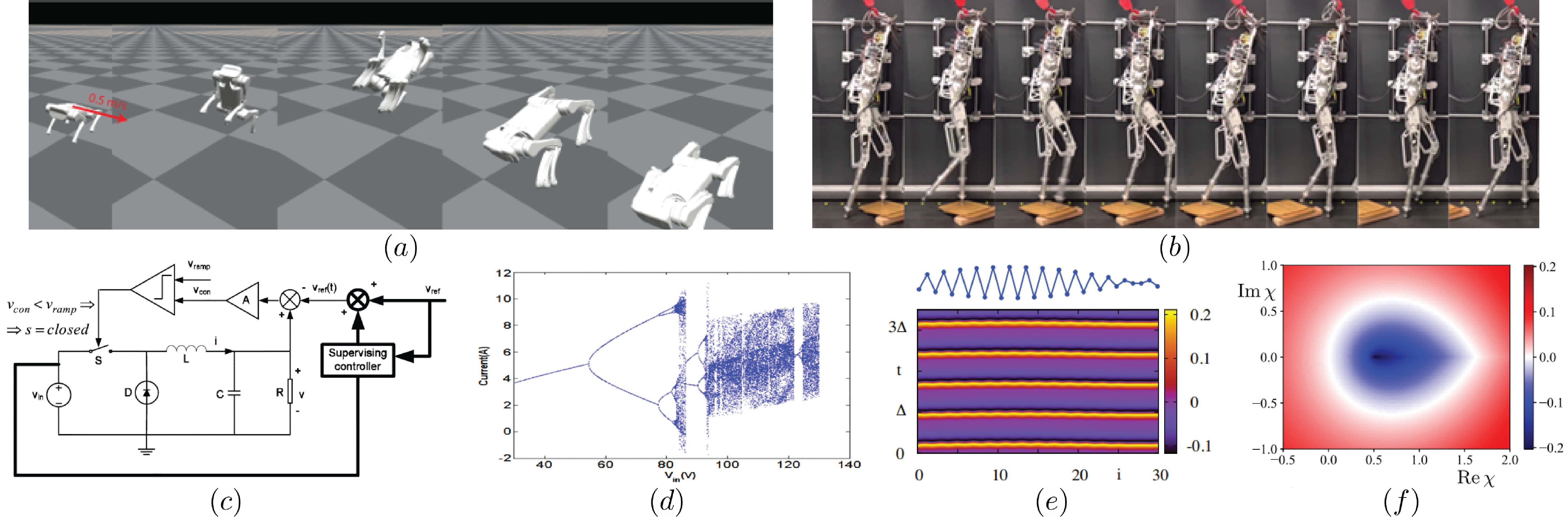
Figure 2: The saltation matrix has been used in many different fields, including the control of legged robots in tasks such as (a) a quadrupedal backflip [14] and (b) robust bipdeal walking [21]; the analysis and control of power circuits such as (c) supervising control of a buck converter [22] and (d) the bifurcation behavior of DC drives [23]; and the modelling of neural activity in the brain such as (e) the stability analysis of a Wilson-Cowan neural mass model[24] and (f) the modelling of synaptic filter behavior[25].

The saltation matrix is a valuable tool for analysis and control in a wide variety of fields such as general bifurcations theory [26, 27, 28, 29, 30], power circuits [31, 32, 33, 22, 23, 34, 35, 36, 37, 38, 39], rigid body systems [40, 41, 42, 43, 44, 45], chemical processing [46], and hybrid neuron models [47, 48, 49, 24, 25, 50]. Fig. 2 shows a few examples that demonstrate the usage of the saltation matrix in the legged robotics, power circuits, and neural modelling literature.

Often, the saltation matrix is used to assess the stability of hybrid dynamical systems, especially for periodic systems [8, 10, 11]. The most popular method for analyzing stability of periodic hybrid systems is to analyze the fundamental matrix solution (as shown in Sec. III-C) which for periodic systems, is called the monodromy matrix[51, 52, 40, 53, 54, 44, 55, 56, 57, 58, 45]. The monodromy matrix is heavily used in the circuits field specifically for determining local stability of switching power converters and determining if bifurcations occur [59, 60, 61, 62, 63, 64, 65, 66, 67, 68, 69, 70, 71, 72, 73, 74, 75, 76, 77, 78, 79, 80, 81, 82, 83, 84, 85, 86, 87, 88, 89, 90]. See [59] for an in depth review for analyzing the stability of switching mode power converters. For more information on bifurcations in periodic systems, see [91, 92, 93, 94] which discuss Lyapunov exponents (the rate of separation of infinitesimally close trajectories) for hybrid systems.

In [16], the saltation matrix components of the monodromy matrix are used to analyze known robotic stabilizing phenomena such as paddle juggling and swing leg retraction. The saltation matrix formulation reveals “shape” parameters, which are terms in the saltation matrix that are independent from the system’s dynamics, but have an effect on the stability of the system. These shape parameters can be optimized to generate stable open loop trajectories for complex hybrid systems that undergo periodic orbits.

A more restrictive but stronger form of stability analysis, known as contraction theory [95], can be done by analyzing the convergence of neighboring trajectories through hybrid events [96] – where global asymptotic convergence is guaranteed if both the continuous-time flow and the saltation matrix are infinitesimally contractive.

Another version of stability was analyzed in [97, 98, 99, 100] as sensitivities to system parameters. Adapted saltation conditions were used to characterize sensitivities across hybrid events. These results were used to formulate and solve optimal design problems.

In addition to stability analysis, saltation matrices are also useful for generating controllers. In optimal control, value functions are propagated along a trajectory to generate feedback controllers. For linear time-varying LQR, sensitivity information about a trajectory is used to schedule optimal gains along that trajectory. To implement optimal trajectory tracking for a hybrid system, [19] utilized the saltation matrix to update the sensitivity equation (as shown in Sec. III-D). Due to the sudden jump from the reset map, the optimal controller will also have a jump in the gain schedule, as first noted in [101]. Other work further expanding and improving on [19] include [17, 102, 103, 18]. A key concept from these works for tracking hybrid trajectories is “reference spreading” or “reference extension” which creates a new references by extending the pre-transition state through the guard and the post-transition state backwards in time. If there is a mode mismatch, the correct reference extension is selected to track.

Using similar value function approximations and reference spreading, [13] proposed a contact implicit trajectory optimization method by extending these ideas to iterative LQR (iLQR). This approach is able to generate both the nominal state trajectory and the feedback controller without having to specify the mode sequence in advance, as in [104, 105, 106, 107], or depend on complementarity constraints that are difficult to solve, as in [108, 109]. Recently, this hybrid iLQR has also been used as an online Model Predictive Controller (MPC) [14].

The saltation matrix has also been used to supplement the concept of hybrid zero dynamics to design robust controllers for bipedal robots. In [21], the norm of the saltation matrix is included in the optimal controller cost function to mitigate the divergent effects of impact.

State estimation uses sensitivity information in an analogous way, where the saltation matrix can be used to propagate covariance through a hybrid transition (Sec. III-D). The first paper to do this is [110], which considers covariance propagation for power-spectral density calculation in circuits. This covariance propagation law was also applied to Kalman filtering for hybrid dynamical systems [12]. This work has also been extended to covariance propagation with noisy guards and uncertainty in the reset map [15]. In [111, 112] hybrid dynamics are considered in an invariant extended Kalman filter for use on lie groups. Using covariance propagation is powerful for state estimation because it efficiently maintains the belief of a distribution through hybrid events. In [12], this “Salted Kalman Filter” runs with comparable accuracy to a hybrid particle filter, e.g. [113], at a fraction of the computation time. The main drawbacks are that it uses a Gaussian approximation, that the entire distribution is propagated instantaneously, and that it is not capable of keeping track of a split distribution that exists near a hybrid transition (whereas non-parametric filters like the particle filter can maintain a non-Gaussian and split distribution).

In cases where multiple guard conditions are met at the same time such as simultaneous leg touchdown, the hybrid event must be analyzed with another tool known as the Bouligand derivative (B-derivative) [114, 115, 116, 117, 52] as the saltation matrix only considers the effects of individual hybrid transition events. The B-derivative can be thought of as a set of composed saltation matrices which capture infinitesimal effects of differing transition sequences. The B-derivative has been used to analyze stability in systems with simultaneous impacts in [115].

TABLE I: Notation used and equation, definition, or section of introduction.

$A$	Linearized vector field matrix, (32)
$\mathbb{COV}$	Covariance
$\mathrm{D}_{*}$	Jacobian w.r.t $*$
$\mathcal{D},D$	Hybrid domain, Def. 1
$\mathbb{E}$	Expectation
$e$	Coefficient of restitution, (69)
$\mathcal{F},F$	Vector field, Def. 1
$f$	Constraint force vector, (63)
$f_{\mathrm{n}},f_{\mathrm{t}}$	Normal and tangential constraint forces, (68)
$\mathcal{G},G,g$	Guard sets and guard function, Def. 1
$\bar{g}$	Linearized guard function, (19)
$H$	Hamiltonian, (154)
h.o.t.	Higher order terms, (10)
$I$	Identity matrix
$\mathrm{I},\mathrm{J}$	Hybrid modes, Def. 1
$i,j$	Hybrid mode indexes, (36)
$J$	Constraint Jacobian, Sec. IV
$\mathcal{J}$	Set of discrete modes, Def. 1
$L$	Limit cycle, Sec. III-C
$\ell$	Loss function, (150)
$M,C,N,\Upsilon$	Mass, Coriolis, nonlinear force, and input matrices, (63)
$M^{\dagger}$, $J^{\dagger}$, $\Lambda^{\dagger}$	Dagger elements for rigid body systems, (64)
$m,n$	Configuration & state space dimensions, Def. 2, Sec. V-A
n, t	Normal or tangential direction constraints, Sec. V-A
$P$	Co-vector quadratic matrix, (42)
$\mathcal{P}$	Poincaré map, Sec. III-C
$p$	Costate, Appendix -D
$Q$	Penalty on state, Appendix -D
$q$, $\dot{q}$, $\ddot{q}$	Configuration, velocity, and acceleration, Sec. IV
$\mathcal{R},R$	Reset map, Def. 1
$\bar{R}$	Linearized reset map, (18)
$\mathbb{R}$	Set of real numbers
$S$	Poincaré section, Sec. III-C
$\mathcal{T}*$	Tangent bundle over *
$T$	Time period, Sec. III-C
$t$	Time, Sec. III
$\widetilde{t}$	Perturbed impact time, Sec. III-B
$\mathrm{U},\mathrm{V},\mathrm{S},\mathrm{C}$	Rigid body modes, Secs. IV, V
$V$	Penalty on input, Appendix -D
$v,\lambda$	Eigenvector and eigenvalue, Sec. IV-C
$u$	Control input, Def. 1
$X$	Random variable, Appendix -C
$x$	State, Def. 1
$x^{*}$	Fixed point, Sec. III-C
$\widetilde{x}$	Perturbed trajectory, Sec. III-B
$\delta x$	Perturbation, (20)
$Z$	Additional terms, (85)
$\Gamma$	Set of discrete transitions, Def. 1
$\Delta$	Discrete timestep, Sec. III-C
$\theta$	Angle of sloped surface, (43)
$\mu$	Floquet exponent III-C
$\mu_{s},\mu_{k}$	Static and kinetic friction coefficient, (68)
$\Xi$	Saltation matrix, (2)
$\rho$	Random variable mean, Appendix -C
$\Sigma$	Covariance, Appendix -C
$\sigma$	Floquet multiplier III-C
$\tau$	Time to impact map, (106)
$\Phi$	Monodromy matrix, (36)
$\phi$	Solutions of the flow, (102)
$\Omega$	Saltation block element, (54)
$0$	Zero matrix
$(*)^{-},(*)^{+}$	Pre-impact and post-impact, Def. 1

III The saltation matrix and how to use it

This section defines the saltation matrix and the broad class of hybrid systems where the saltation matrix applies (Sec. III-A), derives the expression of the saltation matrix using a geometric approach (Sec. III-B), and demonstrates the use of saltation matrices in linear (Sec. III-C) and quadratic forms (Sec. III-D). Table I summarizes the notation used throughout the rest of the paper.

III-A Saltation matrix definition

While there are many definitions of hybrid dynamical systems, e.g. [1, 2, 3, 4], this treatment of the saltation matrix is based on the definition from [13].

Definition 1

A $C^{r}$ hybrid dynamical system, for continuity class $r\in\mathbb{N}_{>0}\cup\{\infty,\omega\}$, is a tuple $\mathcal{H}:=(\mathcal{J},{\mathnormal{\Gamma}},\mathcal{D},\mathcal{F},\mathcal{G},\mathcal{R})$ where the parts are defined as:

1. $\mathcal{J}:=\{\mathrm{I},\mathrm{J},...\}\subset\mathbb{N}$ is the finite set of discrete modes.

2. $\mathnormal{\Gamma}\subseteq\mathcal{J}\times\mathcal{J}$ is the set of discrete transitions forming a directed graph structure over $\mathcal{J}$.

3. $\mathcal{D}:=\amalg_{\mathrm{I}\in\mathcal{J}}$ ${D}_{\mathrm{I}}$ is the collection of domains, where $D_{\mathrm{I}}$ is a $C^{r}$ manifold and the state $x\in D_{\mathrm{I}}$ while in mode $\mathrm{I}$.

4. $\mathcal{F}:=\amalg_{\mathrm{I}\in\mathcal{J}}F_{\mathrm{I}}$ is a collection of $C^{r}$ time-varying vector fields, $F_{\mathrm{I}}:\mathbb{R}\times D_{\mathrm{I}}\to\mathcal{T}D_{\mathrm{I}}$.

5. $\mathcal{G}:=\amalg_{(\mathrm{I},\mathrm{J})\in\mathnormal{\Gamma}}$ $G_{(\mathrm{I},\mathrm{J})}(t)$ is the collection of guard sets, where $G_{(\mathrm{I},\mathrm{J})}(t)\subseteq D_{\mathrm{I}}$ for each $(\mathrm{I},\mathrm{J})\in\mathnormal{\Gamma}$ is defined as a regular sublevel set of a $C^{r}$ guard function, i.e. $G_{(\mathrm{I},\mathrm{J})}(t)=\{x\in D_{\mathrm{I}}|g_{(\mathrm{I},\mathrm{J})}(t,x)\leq 0\}$ and $\mathrm{D}_{x}g_{(\mathrm{I},\mathrm{J})}(t,x)\neq 0\>\>\forall\>\>g_{(\mathrm{I},\mathrm{J})}(t,x)=0$.

6. $\mathcal{R}:\mathbb{R}\times\mathcal{G}\rightarrow\mathcal{D}$ is a $C^{r}$ map called the reset that restricts as $R_{(\mathrm{I},\mathrm{J})}:=\mathcal{R}|_{G_{(\mathrm{I},\mathrm{J})(t)}}:G_{(\mathrm{I},\mathrm{J})}(t)\rightarrow D_{\mathrm{J}}$ for each $(\mathrm{I},\mathrm{J})\in\mathnormal{\Gamma}$.

Note that this definition incorporates the control input $u(t,x)$ into the dynamics $\mathcal{F}$ as $\mathcal{F}(t,x,u(t,x))\rightarrow\mathcal{F}(t,x)$.

Fig. 3 shows an example hybrid system with a hybrid execution consisting of a starting point $x(0)$ in ${D}_{\mathrm{I}}$ flowing with dynamics ${F}_{\mathrm{I}}$ and reaching the guard condition $g_{(\mathrm{I},\mathrm{J})}(t,x)=0$ at time $t$, applying the reset map $R_{(\mathrm{I},\mathrm{J})}(t,x)$ resetting into ${D}_{\mathrm{J}}$ and then flowing with the new dynamics ${F}_{\mathrm{J}}$. Denote $t^{-}$ as the instant before the reset map is applied, $t^{+}$ the instant after the reset map is applied, and $x(t^{\pm})=x^{\pm}$ the limiting value of the signal $x$ from the left $(-)$ or right $(+)$.

The goal in this paper is to understand how perturbations about a nominal trajectory evolve over time. For smooth systems, it is well known that perturbations about a nominal trajectory can be approximated to first order using the derivative of the dynamics $F(t,x)$ with respect to state:

$$\delta\dot{x}=\mathrm{D}_{x}F(t,x)\delta x$$ (1)

Hybrid systems with time triggered reset maps can be similarly analyzed using the Jacobian of the reset map, $\delta x^{+}=\mathrm{D}_{x}R(t,x)\delta x^{-}$. However, the Jacobian of the reset map does not account for differences that are introduced from time-to-impact variations in systems with event driven resets, where the differences in dynamics in the two hybrid modes must be considered. The saltation matrix, e.g. [8, Eq. 3.5], [9, Pg. 118 Eq. 6], [10, Eq. 7.65], or [96, Prop. 2], accounts for these terms to capture how perturbations are mapped through event-driven hybrid transitions to the first order. From here on, the term hybrid transition/system refers to this event-driven class.

Definition 2

The saltation matrix for transition from mode I to mode J is the first order approximation of the variational update at hybrid transitions from mode I to J, defined as:

$$\Xi_{(\mathrm{I},\mathrm{J})}:=\mathrm{D}_{x}R^{-}+\frac{\left(F^{+}_{\mathrm{J}}-\mathrm{D}_{x}R^{-}F^{-}_{\mathrm{I}}-\mathrm{D}_{t}R^{-}\right)\mathrm{D}_{x}g^{-}}{\mathrm{D}_{t}g^{-}+\mathrm{D}_{x}g^{-}F^{-}_{\mathrm{I}}}$$ (2)

Note that the matrix multiplication in (2) results in an outer-product between the terms in the parentheses and $\mathrm{D}_{x}g^{-}$ to get a rank-1 correction to the Jacobian of the reset map. The saltation matrix is an $n_{\mathrm{J}}\times n_{\mathrm{I}}$ matrix, where $n_{\mathrm{I}}$ is the dimension of the states in domain $D_{\mathrm{I}}$ and $n_{\mathrm{J}}$ is the dimension of the states in domain $D_{\mathrm{J}}$. The following evaluations are made for the terms in the saltation matrix:

$$F^{-}_{\mathrm{I}} :=F_{\mathrm{I}}(t^{-},x(t^{-}))$$ (3)

$$F^{+}_{\mathrm{J}} :=F_{\mathrm{J}}(t^{+},x(t^{+}))$$ (4)

$$x(t^{+}) :={R}_{(\mathrm{I},\mathrm{J})}(t^{-},x(t^{-}))$$ (5)

$$\mathrm{D}_{x}R^{-} :=\mathrm{D}_{x}{R}_{(\mathrm{I},\mathrm{J})}(t^{-},x(t^{-}))$$ (6)

$$\mathrm{D}_{t}R^{-} :=\mathrm{D}_{t}{R}_{(\mathrm{I},\mathrm{J})}(t^{-},x(t^{-}))$$ (7)

$$\mathrm{D}_{x}g^{-} :=\mathrm{D}_{x}{g}_{(\mathrm{I},\mathrm{J})}(t^{-},x(t^{-}))$$ (8)

$$\mathrm{D}_{t}g^{-} :=\mathrm{D}_{t}{g}_{(\mathrm{I},\mathrm{J})}(t^{-},x(t^{-}))$$ (9)

Note that $\mathrm{D}_{t}$ in (7) and (9) refers to the derivative with respect to the first coordinate (and not the time dependence of $x$, which is captured by other terms).

The saltation matrix maps perturbations to the first order from pre-transition $\delta x(t^{-})$ to post-transition $\delta x(t^{+})$ as:

$$\delta x(t^{+})=\Xi_{(\mathrm{I},\mathrm{J})}\delta x(t^{-})+\text{h.o.t.}$$ (10)

where h.o.t. represents higher order terms.

The saltation matrix in (2) is suitable when the following assumptions are true, as listed in [96]

1. Guards and resets are differentiable

2. Trajectories cannot undergo an infinite number of resets in finite time (no Zeno)

3. Trajectories must be transverse to the guard at an event:

   $$\frac{d}{dt}g_{(\mathrm{I},\mathrm{J})}(t,x(t))=\mathrm{D}_{t}g^{-}+\mathrm{D}_{x}g^{-}F_{\mathrm{I}}^{-}<0$$ (11)

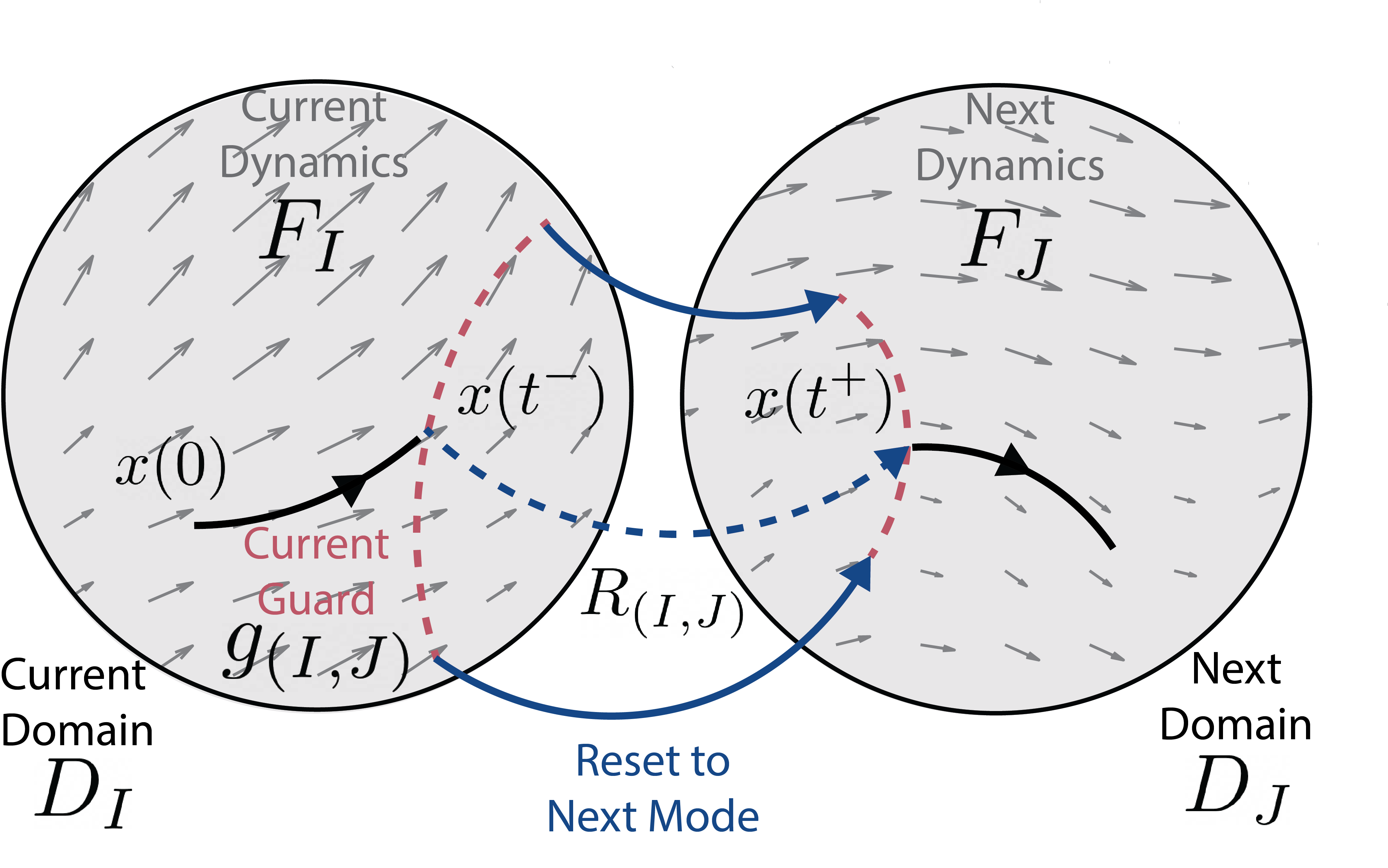
Figure 3: An example 2 mode hybrid system where the domains are shown in black circles $D$, the dynamics are shown with gray arrows $F$, the guard for the current domain is shown in red dashed $g$, and the reset from the current mode to the next mode is shown in blue $R$.

The saltation matrix relies on differentiating the guards and resets so they must be differentiable. Excluding Zeno conditions ensures we avoid computing infinite saltation matrices in finite time, which would clearly be unsound for analysis. Transversality ensures that neighboring trajectories impact the same guard unless the impact point lies on any other guard surface, in which case the Bouligand derivative is the appropriate analysis tool [114, 115, 116, 117, 52]. Transversality also ensures the denominator in (2) does not approach zero.

In some cases, the saltation matrix for a hybrid transition can become an identity transformation. Knowing when the saltation matrix is identity is useful to simplify computation and analysis. The most common reason for a saltation matrix to become identity is if both of these conditions are true:

1. the reset map is an identity transformation, $R=I_{n\times n}$, where $n$ is the dimension of the state $x$ in both $D_{\mathrm{I}}$ and $D_{\mathrm{J}}$

2. the dynamics in both modes are the same before and after impact, $F^{-}_{\mathrm{I}}=F^{+}_{\mathrm{J}}$:

$$\left.\begin{array}[]{c}R=I_{n\times n}\\ F^{-}_{\mathrm{I}}=F^{+}_{\mathrm{J}}\end{array}\right\}\implies\Xi=I_{n\times n}$$ (14)

An example of such a transition is a foot lifting off from the ground. If the reset map is an identity transformation, then $\mathrm{D}_{x}R$ is also identity and $\mathrm{D}_{t}R$ is zero. Using these conditions to simplify the expression in (2) gives:

$$\Xi_{(\mathrm{I},\mathrm{J})}=I_{n\times n}+\frac{\left(F^{+}_{\mathrm{J}}-I_{n\times n}F^{-}_{\mathrm{I}}-0_{n\times n}\right)\mathrm{D}_{x}g^{-}}{\mathrm{D}_{t}g^{-}+\mathrm{D}_{x}g^{-}F^{-}_{\mathrm{I}}}=I_{n\times n}$$ (15)

III-B Saltation matrix derivation

In this section, the derivation of the saltation matrix (2) is presented, following the geometric derivation from [10] with the addition of reset maps. There are many alternate ways to derive (2): a derivation using the chain rule is included in Appendix -A and a derivation using a double limit can be found in [96].

Figure 4: Linearizations made about the nominal trajectory shown in black where a perturbation is shown in yellow and the perturbed trajectory is shown in blue. At $a)$ describes $\vec{v}=F_{\mathrm{I}}^{-}\delta t+\delta x(t^{-})$. At $b)$ the guard condition is $0=\mathrm{D}_{x}g^{-}(\delta x(t^{-})+F_{\mathrm{I}}^{-}\delta t)$. At $c)$ $\delta x(\widetilde{t}^{+})$ is $\mathrm{D}_{x}R^{-}\vec{v}-F_{\mathrm{J}}^{+}\delta t$. Here $\delta t$ is positive (late transition) and for the purposes of this figure it is assumed that the system is autonomous, so the $\mathrm{D}_{t}g$ and $\mathrm{D}_{t}R$ terms drop out.

Suppose the nominal trajectory of interest is $x(t)$ as shown in Fig. 4. The trajectory starts in mode I and goes through a hybrid transition to mode J at time $t$. The saltation matrix is a first-order approximation, so the flow is treated as a constant in each mode, evaluated at time $t^{\pm}$ as in (3) and (4) such that for an infinitesimal timestep $\delta t$:

$$x(t^{-})=x(t^{-}-\delta t)+F_{\mathrm{I}}^{-}\delta t\qquad\textrm{in mode I}$$ (16)

$$x(t^{+}+\delta t)=x(t^{+})+F_{\mathrm{J}}^{+}\delta t\qquad\textrm{in mode J}$$ (17)

The reset and guard are also linearized at $t^{-}$ as in (6) and (8), such that

$$\bar{R}(t^{-}+\delta t,x+\delta x)=R_{(\mathrm{I},\mathrm{J})}(t^{-},x(t^{-}))+\mathrm{D}_{x}R^{-}\delta x+\mathrm{D}_{t}R^{-}\delta t$$ (18)

$$\bar{g}(t^{-}+\delta t,x+\delta x)=g_{(\mathrm{I},\mathrm{J})}(t^{-},x(t^{-}))+\mathrm{D}_{x}g^{-}\delta x+\mathrm{D}_{t}g^{-}\delta t$$ (19)

where $\bar{R}$ and $\bar{g}$ are the linear maps.

Trajectories that are perturbed $\delta x$ away are labeled as $\widetilde{x}$. Perturbations can lead to changes in the impact time, which we describe with the infinitesimal time difference $\delta t:=\widetilde{t}-t$ where $t$ is the original impact time and $\widetilde{t}$ is the perturbed impact time. If $\delta t>0$ then the perturbed transition is late and the solution stays in the previous hybrid mode longer, while if $\delta t<0$ then the perturbed solution transitions early. For simplicity of notation, assume the perturbed trajectory reaches the guard surface late, but the analysis also works for early transitions, resulting in the same expression (2), as shown in Appendix -B.

Define the perturbation at the pre-impact time of the nominal trajectory $t^{-}$ and the post-impact time of the perturbed trajectory $\widetilde{t}^{+}$ as:

$$\delta x(t^{-}):=\widetilde{x}(t^{-})-x(t^{-})$$ (20)

$$\delta x(\widetilde{t}^{+}):=\widetilde{x}(\widetilde{t}^{+})-x(\widetilde{t}^{+})$$ (21)

where $\widetilde{x}(t^{-})$ is the perturbed trajectory following the previous mode dynamics until time $t^{-}$. Next, we can write (21) in terms of the nominal trajectory at time of impact $x(t^{-})$ and just after impact $x(t^{+})$. Using (20) and (16), $\widetilde{x}(\widetilde{t}^{-})$ can be written in terms of the flow before impact $F_{\mathrm{I}}^{-}\delta t$ and the perturbation before impact $\delta x(t^{-})$:

$$\widetilde{x}(\widetilde{t}^{-})=x(t^{-})+\delta x(t^{-})+F_{\mathrm{I}}^{-}\delta t$$ (22)

Note that we denote the expression $\delta x(t^{-})+F_{\mathrm{I}}^{-}\delta t$ as $\vec{v}$ in Fig. 4 Eq. a. By using the linearized reset map (18) and the perturbation expressed in terms of the nominal trajectory (22), the reset at $\widetilde{x}(\widetilde{t}^{-})$ can be evaluated in terms of the nominal state $x(t^{-})$, the initial perturbation $\delta x(t^{-})$, and the difference in impact time $\delta t$

$$\widetilde{x}(\widetilde{t}^{+})=R(t^{-},{x}(t^{-}))+\mathrm{D}_{x}R^{-}\left(\delta x(t^{-})+F^{-}_{\mathrm{I}}\delta t\right)+\mathrm{D}_{t}R^{-}\delta t$$ (23)

The final term in (21) is obtained by using the constant flow after the reset (16) to calculate ${x}(\widetilde{t}^{+})$:

$${x}(\widetilde{t}^{+}) =R(t^{-},x(t^{-}))+F^{+}_{\mathrm{J}}\delta t$$ (24)

By combining (21), (23), and (24), $\delta x(\widetilde{t}^{+})$ can now be written as a linear function of $\delta x(t^{-})$ and $\delta t$ :

$$\delta x(\widetilde{t}^{+}) =R(t^{-},{x}(t^{-}))+\mathrm{D}_{x}R^{-}\left(\delta x(t^{-})+F^{-}_{\mathrm{I}}\delta t\right)$$ (25)

$$\quad+\mathrm{D}_{t}R^{-}\delta t-\left(R(t^{-},x(t^{-}))+F^{+}_{\mathrm{J}}\delta t\right)$$

$$=\mathrm{D}_{x}R^{-}\delta x(t^{-})+\left(\mathrm{D}_{x}R^{-}F^{-}_{\mathrm{I}}+\mathrm{D}_{t}R^{-}-F^{+}_{\mathrm{J}}\right)\delta t$$ (26)

This step is highlighted by the vector addition in Fig. 4 Eq. c.

Next, we solve for $\delta t$ as a function of $\delta x(t^{-})$. The linear property of the guard (19) and the perturbation expressed in terms of the nominal trajectory (22) are used to rewrite the guard evaluated at $\widetilde{x}(\widetilde{t}^{-})$ as a function of the nominal (and noting that $g(t^{-},{x}({t}^{-}))=0$):

$$0 =g(t^{-},{x}({t}^{-}))+\mathrm{D}_{x}g^{-}(\delta x(t^{-})+F_{\mathrm{I}}^{-}\delta t)+\mathrm{D}_{t}g^{-}\delta t$$ (27)

$$=\mathrm{D}_{x}g^{-}\delta x(t^{-})+(\mathrm{D}_{x}g^{-}F^{-}_{\mathrm{I}}+\mathrm{D}_{t}g^{-})\delta t$$ (28)

This expansion shows up in Fig. 4 as Eq. b. Writing $\delta t$ as a function of $\delta x(t^{-})$ gives:

$$\delta t=-\frac{\mathrm{D}_{x}g^{-}}{\mathrm{D}_{x}g^{-}F^{-}_{\mathrm{I}}+\mathrm{D}_{t}g^{-}}\delta x(t^{-})$$ (29)

Substituting this $\delta t$ into (26) and solving for $\delta x(\widetilde{t}^{+})$ in terms of $\delta x(t^{-})$:

$$\delta x(\widetilde{t}^{+}) =\mathrm{D}_{x}R^{-}\delta x(t^{-})$$ (30)

$$\quad+\frac{\left(F^{+}_{\mathrm{J}}-\mathrm{D}_{x}R^{-}F^{-}_{\mathrm{I}}-\mathrm{D}_{t}R^{-}\right)\mathrm{D}_{x}g^{-}}{\mathrm{D}_{x}g^{-}F^{-}_{\mathrm{I}}+\mathrm{D}_{t}g^{-}}\delta x(t^{-})$$

$$=\Xi_{(\mathrm{I},\mathrm{J})}\delta x(t^{-})$$ (31)

where $\Xi$ is the saltation matrix, as in (10).

III-C Linear forms for the saltation matrix

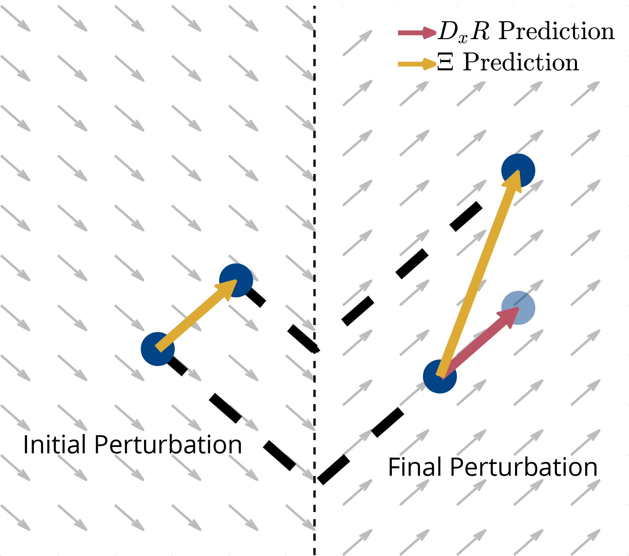
Figure 5: Constant flow hybrid system with identity reset map. The Jacobian of the reset map $\mathrm{D}_{x}R$ predicts no variational changes whereas using the saltation matrix $\Xi$ predicts the correct variational changes.

Understanding how perturbed trajectories behave near a trajectory of interest is crucial for many algorithms which rely on linearizations. The sensitivity equation describes how these perturbations evolve over time. For a hybrid system, the time evolution simply applies the standard smooth sensitivity equation, based on the Jacobian of the flow (1), for the smooth dynamics and the saltation matrix equation when a hybrid transition occurs (10). For a transition from mode I to mode J at time $t^{-}$, the sensitivity is described by:

$$\delta\dot{x}(t) =A_{\mathrm{I}}\delta x(t)\>\> s.t. \>\>t\leq t^{-}$$ (32)

$$\delta x(t^{+}) =\Xi_{(\mathrm{I},\mathrm{J})}\delta x(t^{-})\>\> s.t. \>\>t=t^{-}$$ (33)

$$\delta\dot{x}(t) =A_{\mathrm{J}}\delta x(t)\>\> s.t. \>\>t\geq t^{+}$$ (34)

where $A_{\mathrm{I}}:=\mathrm{D}_{x}F_{\mathrm{I}}(t,x)$ represents the Jacobian of the dynamics with respect to state. An example is shown in Fig. 5, where the sensitivity is updated only by the saltation matrix because the flows are constant in both modes ($A$ is identity). Instead, it is the difference in mode timing that determines the change in sensitivity from the initial to final state. If the Jacobian of the reset (which is also identity) is used instead of the saltation matrix, the prediction is incorrect. Sensitivity of hybrid systems is extensively analyzed in [31] and [19].

Many algorithms consider finite, discrete timesteps. This makes the analysis slightly different, since the hybrid transition will most likely not occur exactly at the boundary of a discrete timestep. In this case, a “sandwich” method is utilized, where 3 (or more) smaller discrete updates are applied during a timestep in which has a hybrid transition. Consider a time interval from $t_{k}$ to $t_{k+1}:=t_{k}+\Delta$ over which a single reset occurs at time $t_{k}+\Delta_{1}$. The system spends $\Delta_{1}$ time in the first mode and $\Delta_{2}:=\Delta-\Delta_{1}$ in the second mode. Let $A_{\mathrm{I},\Delta}$ be the Jacobian of the dynamics discretized to time duration $\Delta$. Then a discrete approximation of the forward dynamics is:

$$\delta x(t_{k+1})=A_{\mathrm{J},\Delta_{2}}\Xi_{(\mathrm{I},\mathrm{J})}A_{\mathrm{I},\Delta_{1}}\delta x(t_{k})$$ (35)

which holds to first order. This result comes from the fundamental matrix solution [10, Eq. 7.22].

Extending this idea, consider a periodic orbit of period $T$, such that $x(t)=x(t+T)$. In this case, the fundamental matrix solution is called the monodromy matrix. If the orbit passes through $j$ modes labeled $i=1,2,\dots,j$, with mode periods $T_{i}$, then we define the monodromy matrix $\Phi$, [10, Eq. 7.28], [118, Eq. 1], and [55, Eq. 12]:

$$\Phi=\Xi_{(j,1)}A_{j,T_{j}}\Xi_{(j-1,j)}A_{j-1,T_{j-1}}\cdots\,\Xi_{(1,2)}A_{1,T_{1}}$$ (36)

$$\delta x(t+T)=\Phi\delta x(t)$$ (37)

which holds to first order. This monodromy matrix captures the change in perturbations from one cycle through the orbit to the next and the eigenvalues (called Floquet multipliers [10]) determine the stability of the trajectory. Namely, if the eigenvalues all have magnitude less than one then the system is asymptotically stable [10].

Related to the monodromy matrix, a common technique to analyze stability of periodic systems is to analyze the return/Poincaré map [10]. A Poincaré map $\mathcal{P}(x)$ converts the continuous-time system to a discrete map. For an autonomous system with $n$ states and a limit cycle $L$, the Poincaré map is defined about a fixed point $x^{*}$ on $L$ and an $n-1$ dimensional hyper-plane transverse to the flow $F$ called the Poincaré section $S$, with $x^{*}\in S$. The Poincaré map captures how points move along the Poincaré section after one cycle ($\mathcal{P}:S\mapsto S$). Stability of the fixed point is often computed by taking the Jacobian of the Poincaré map and analyzing its eigenvalues. If the eigenvalues are less than one (the requirements for stability for a discrete system), the fixed point $x^{*}$ is stable.

Note that for the autonomous case, the dimensionality of the system is reduced by one due to the embedding. For the non-autonomous case, a Poincaré section in state space cannot be defined because it does not regard the dependency on time. Instead, the trajectory is augmented with a periodic time coordinate on $S^{1}$, and the Poincaré section is now defined to be at the end of each period $T$. In this case, the Poincaré map and its Jacobian are in the full $n$ space, as the Poincaré section is defined on the added time coordinate.

Consider a monodromy matrix for a cycle that starts and ends at the fixed point $x^{*}$ for one cycle. In the autonomous case, the monodromy matrix has the same eigenvalues as the Jacobian of the Poincaré map with an additional eigenvalue equal to one. This is because the monodromy matrix is still in the full $n$ space, and perturbations along the direction of the flow are invariant. In the non-autonomous case, the monodromy matrix and the Jacobian of the Poincaré map are equivalent, so sometimes the monodromy matrix is defined simply to be the Jacobian of the Poincaré map [59].

If the system is autonomous and periodic, using the Poincaré map might be more practical because the analysis is simplified by the reduction of a state variable, e.g. as shown for passive dynamic walkers [119]. However, the monodromy matrix can be generalized to the fundamental matrix solution for analysis of non-cyclical behaviors, which the Poincaré map can not. This is especially important when designing dynamic behaviors that are drastically different like for parkour or dynamic grasps.

Also closely related to Floquet multipliers are Lyapunov exponents [92, 93, 94]. For a given Floquet multiplier $\sigma$, it can be written in the form $\sigma=e^{\mu T}$ where $\mu$ is the Floquet exponent and the real part of $\mu$ is the Lyapunov exponent [120]. If all Lyapunov exponents are negative, $\sigma<1$ and the trajectory is asymptotically stable.

III-D Quadratic forms for the saltation matrix

Similar to linear forms, quadratic forms are often used in algorithms which rely on linearizations. Examples of such algorithms include the well-known Kalman filter and LQR controller. There are 2 main updates this section covers: the quadratic form of the vector (covariance) and the co-vector (value approximation).

For covariances, recall that the update law for covariance $\Sigma$ through a discretized smooth system, with timesteps $\Delta$, is:

$$\Sigma(t_{k+1}) =A_{\Delta}\Sigma(t_{k})A^{T}_{\Delta}$$ (38)

e.g. as in [121, Eqn. 1.10] or [122, Eqn. 6]. Similarly, at hybrid transitions, the saltation matrix applies in an analogous way (see derivation in Appendix -C):

$$\Sigma(t^{+}) =\Xi_{(\mathrm{I},\mathrm{J})}\Sigma(t^{-})\Xi_{(\mathrm{I},\mathrm{J})}^{T}$$ (39)

[110, Eqn. 17], [12, Eqn. 7], which holds to first order. As with linear forms, the sandwich method (35) can be applied to retrieve the covariance propagation for an entire discrete timestep:

$$\Sigma(t_{k+1})=A_{\mathrm{J},\Delta_{2}}\Xi_{(\mathrm{I},\mathrm{J})}A_{\mathrm{I},\Delta_{1}}\Sigma(t_{k})A_{\mathrm{I},\Delta_{1}}^{T}\Xi_{(\mathrm{I},\mathrm{J})}^{T}A_{\mathrm{J},\Delta_{2}}^{T}$$ (40)

[12, Eqn. 19]. An example is shown in Fig. 6, where the covariance is once again updated only by the saltation matrix because the flows are constant in both modes ($A$ is identity). If the Jacobian of the reset is used instead, the incorrect covariance is predicted. Algorithms, such as a Kalman filter [12], that propagate covariances with the dynamics can utilize this update law.

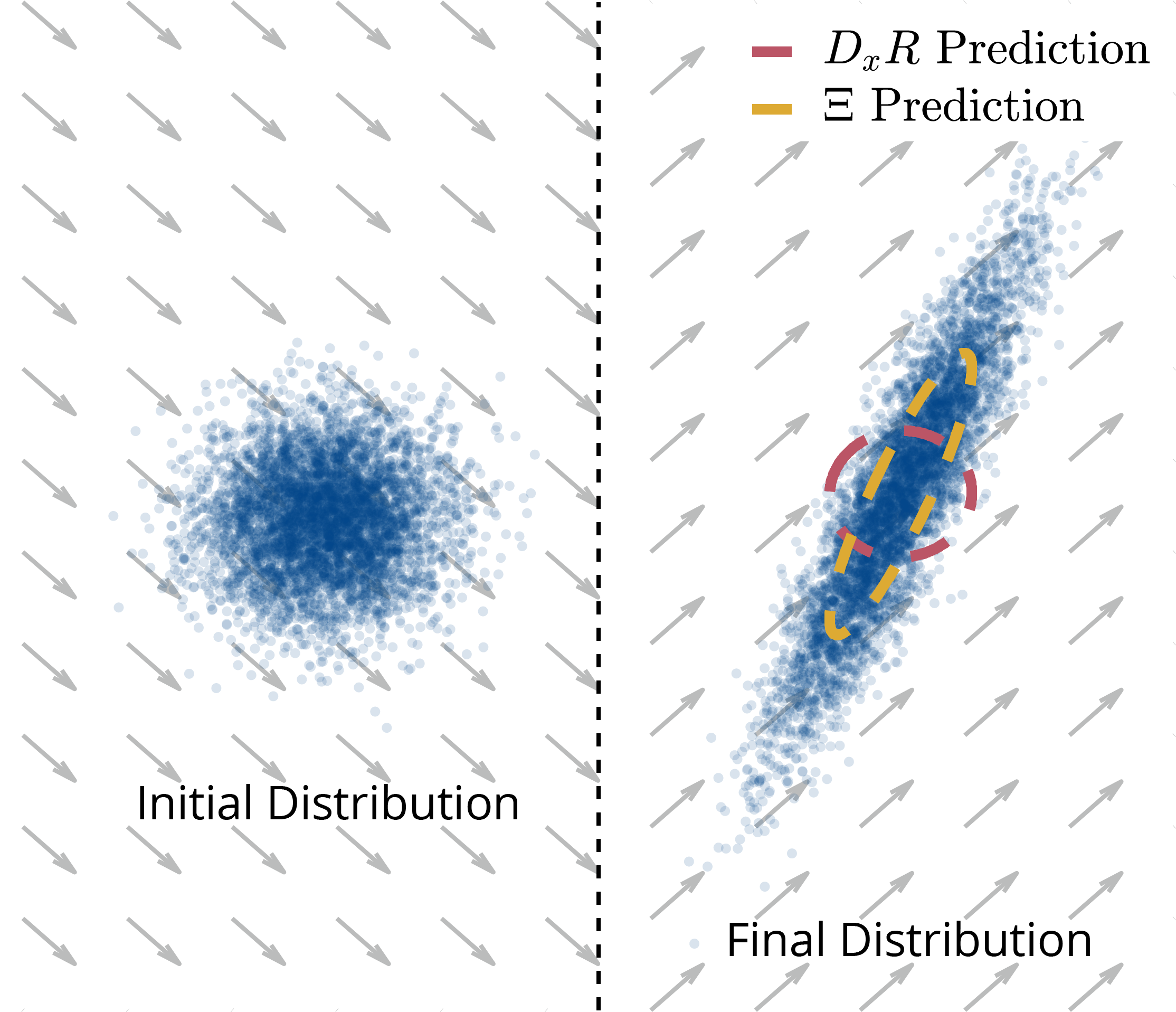
Figure 6: Constant flow hybrid system with identity reset map. The Jacobian of the reset map $\mathrm{D}_{x}R$ predicts no covariance change whereas using the saltation matrix $\Xi$ predicts the correct covariance.

In the case of propagating a quadratic form of a co-vector, the matrix transpose terms flip sides similar to how a co-vector quadratic form propagates in the smooth domain:

$$P(t_{k})=A^{T}_{\Delta}P(t_{k+1})A_{\Delta}$$ (41)

as in [123, Eqn. 3.40]. The co-vector propagation law for the hybrid transition uses the saltation matrix in an analogous way (see derivation in Appendix -D):

$$P(t^{-})=\Xi_{(\mathrm{I},\mathrm{J})}^{T}P(t^{+})\Xi_{(\mathrm{I},\mathrm{J})}$$ (42)

[17, Eqn. 23], [13, Eqn. 31]. The main application of the co-vector case is in the update to the Riccati equation or Bellman update, e.g. in LQR [13, 17].

IV Example: Calculating the saltation matrix for a ball dropping on a slanted surface

One of the simplest examples of a hybrid system is a 2D point mass (ball) falling and hitting a flat surface, as shown in Fig. 1. Intuitively, the impact should eliminate variations normal to the constraint in both position and velocity. This section presents the computation of the saltation matrix for this example and how it confirms the collapse of variations normal to the constraint.

IV-A Dynamics definition

Here, the system’s dynamics are summarized for the 2D point mass, with an in-depth derivation for a general rigid body system given in Sec. V. The horizontal and vertical positions as well as their velocities are defined to be the states of the system, $x=[q^{T},\dot{q}^{T}]^{T}=[q_{1},q_{2},\dot{q}_{1},\dot{q}_{2}]^{T}$. The ball has mass $m$ and acceleration due to gravity $a_{g}$. For the sake of demonstrating how inputs are handled, the ball is fully actuated with control inputs along the configuration coordinates $[u_{1},u_{2}]^{T}$. Two cases of friction are considered, one that assume frictionless sliding when in contact with the surface (i.e. the kinetic friction coefficient is zero, $\mu_{k}=0$) and one where the friction is sufficient to prevent sliding, i.e. the ball sticks to a spot.

The ball impacts a sloped surface parameterized by an angle $\theta$, where the position constraint is defined by the guard function:

$$g_{(\mathrm{U},\mathrm{S})}(t,x)=\sin{(\theta)}q_{1}+\cos{(\theta)}q_{2}=0$$ (43)

where U is the unconstrained mode and S is the constrained sliding mode (the ball can slide tangentially along the constraint surface). The resulting velocity constraint Jacobian $J_{\mathrm{S}}$ in the sliding mode is:

$$J_{\mathrm{S}}(q)=\mathrm{D}_{q}g_{(\mathrm{U},\mathrm{S})}(t,x)=\begin{bmatrix}\sin{(\theta)}&\cos{(\theta)}\end{bmatrix},\quad\>s.t.\>J_{\mathrm{S}}\dot{q}=0$$ (44)

The unconstrained mode dynamics are defined by ballistic motion:

$$F_{\mathrm{U}}(t,x)=\begin{bmatrix}\dot{q}_{1}&\dot{q}_{2}&\frac{u_{1}}{m}&\frac{u_{2}-a_{g}m}{m}\end{bmatrix}^{T}$$ (45)

The hybrid guard for impact is defined by the constraint $g_{(\mathrm{U},\mathrm{S})}(q)\leq 0$, i.e when the constraint is met the impact occurs. The reset map is defined by plastic impact, which enforces the velocity constraint:

$$R_{(\mathrm{U},\mathrm{S})}(t,x)=\begin{bmatrix}q_{1}\\ q_{2}\\ \dot{q}_{1}\,{\cos^{2}\left(\theta\right)}-\dot{q}_{2}\,\cos\left(\theta\right)\,\sin\left(\theta\right)\\ \dot{q}_{2}\,{\sin^{2}\left(\theta\right)}-\dot{q}_{1}\,\sin\left(\theta\right)\,\cos\left(\theta\right)\end{bmatrix}$$ (46)

The constrained mode dynamics are found by solving the ballistic dynamics while maintaining the velocity constraint:

$$F_{\mathrm{S}}(t,x)=\begin{bmatrix}\dot{q}_{1}\\ \dot{q}_{2}\\ \frac{u_{1}\,{\cos^{2}\left(\theta\right)}}{m}-\frac{u_{2}\,\cos\left(\theta\right)\,\sin\left(\theta\right)}{m}+\frac{g\,m\,\cos\left(\theta\right)\,\sin\left(\theta\right)}{m}\\ -\frac{u_{1}\,\cos\left(\theta\right)\,\sin\left(\theta\right)}{m}+\frac{u_{2}\,{\sin^{2}\left(\theta\right)}}{m}-\frac{g\,m\,{\sin^{2}\left(\theta\right)}}{m}\end{bmatrix}$$ (47)

In the case of sticking friction in a third mode $\mathrm{C}$, there is a no slip condition added to (44):

$$J_{\mathrm{C}}=\begin{bmatrix}-\cos(\theta)&\sin(\theta)\\ \sin(\theta)&\cos(\theta)\end{bmatrix},\quad\>s.t.\>J_{\mathrm{C}}\dot{q}=0$$ (48)

such that the constrained dynamics become:

$$\dot{x}=F_{\mathrm{C}}(t,x)=\begin{bmatrix}\dot{q}_{1}&\dot{q}_{2}&0&0\end{bmatrix}^{T}$$ (49)

The reset map eliminates all velocities:

$$R{(\mathrm{U},\mathrm{C})}(t,x)=\begin{bmatrix}q_{1}&q_{2}&0&0\end{bmatrix}^{T}$$ (50)

Note that this mode is fully constrained and the ball will just stick to the surface (as $\dot{q}=0$ after impact).

IV-B Saltation matrix calculation

To compute the saltation matrix, the Jacobians of the guard and reset map with respect to state must be computed. The Jacobian of the guard is simply the velocity constraint Jacobian padded with zeros for each velocity coordinate:

$$\mathrm{D}_{x}g_{(\mathrm{U},\mathrm{S})}(t,x)=\begin{bmatrix}J_{\mathrm{S}}&0_{1\times 2}\end{bmatrix}=\begin{bmatrix}\sin(\theta)&\cos(\theta)&0&0\end{bmatrix}$$ (51)

The Jacobian of the reset map is:

$$\mathrm{D}_{x} R_{(\mathrm{U},\mathrm{S})}(t,x)=$$ (52)

$$\begin{bmatrix}1&0&0&0\\ 0&1&0&0\\ 0&0&{\cos^{2}\left(\theta\right)}&-\cos\left(\theta\right)\,\sin\left(\theta\right)\\ 0&0&-\cos\left(\theta\right)\,\sin\left(\theta\right)&\sin^{2}\left(\theta\right)\end{bmatrix}$$

The saltation matrix is then computed by substituting in each component, (45)–(52), into the definition, (2), to get:

$$\Xi_{(\mathrm{U},\mathrm{S})}=\begin{bmatrix}\Omega_{(\mathrm{U},\mathrm{S})}&0_{2\times 2}\\ 0_{2\times 2}&\Omega_{(\mathrm{U},\mathrm{S})}\end{bmatrix}$$ (53)

where $\Omega_{(\mathrm{U},\mathrm{S})}$ is a block element consisting of:

$$\Omega_{(\mathrm{U},\mathrm{S})}=\begin{bmatrix}\cos^{2}\left(\theta\right)&-\cos\left(\theta\right)\,\sin\left(\theta\right)\\ -\cos\left(\theta\right)\,\sin\left(\theta\right)&\sin^{2}\left(\theta\right)\end{bmatrix}$$ (54)

For the sticking saltation matrix, similar calculations are made as in the sliding case:

$$\mathrm{D}_{x}g{(\mathrm{U},\mathrm{C})}(t,x)=\begin{bmatrix}\sin(\theta)&\cos(\theta)&0&0\end{bmatrix}$$ (55)

Note that the guard condition is the same, which results in having the same Jacobian of the guard as the sliding case. The Jacobian of the reset map is:

$$\mathrm{D}_{x}R_{(\mathrm{U},\mathrm{C})}(t,x)=\begin{bmatrix}1&0&0&0\\ 0&1&0&0\\ 0&0&0&0\\ 0&0&0&0\end{bmatrix}$$ (56)

The resulting saltation matrix becomes:

$$\Xi_{(\mathrm{U},\mathrm{C})}=\begin{bmatrix}\Omega_{(\mathrm{U},\mathrm{C})}&0_{2\times 2}\\ 0_{2\times 2}&0_{2\times 2}\end{bmatrix}$$ (57)

where $\Omega_{(\mathrm{U},\mathrm{C})}$ is a block element consisting of:

$$\Omega_{(\mathrm{U},\mathrm{C})}=\frac{1}{{\dot{q}_{2}\,\cos\left(\theta\right)+\dot{q}_{1}\,\sin\left(\theta\right)}}\begin{bmatrix}\dot{q}_{2}\,\cos\left(\theta\right)&-\dot{q}_{1}\,\cos\left(\theta\right)\\ -\dot{q}_{2}\,\sin\left(\theta\right)&\dot{q}_{1}\,\sin\left(\theta\right)\end{bmatrix}$$ (58)

IV-C Saltation matrix analysis

Interestingly, the saltation matrix for the sliding case $\Xi_{(\mathrm{U},\mathrm{S})}$ is a block diagonal matrix with a repeating block element, shown in (53)–(54). This implies that the variations in position are mapped equivalently to variations in velocity. The eigenvalues and corresponding eigenvectors of this block are:

$$\lambda_{0} =0, \lambda_{1} =1$$

$$v_{0} =\begin{bmatrix}\sin(\theta)\\ \cos(\theta)\end{bmatrix}, v_{1} =\begin{bmatrix}-\cos{\theta}\\ \sin{\theta}\end{bmatrix}$$ (59)

The first eigenvalue is zero, so any variation in the direction of its eigenvector is eliminated. Note that this eigenvector is exactly the velocity constraint Jacobian, $J_{\mathrm{S}}=[\sin(\theta),\cos(\theta)]$. Thus, variations off the constraint for both position and velocity are zeroed out, i.e. there are no variations normal to the surface once impact is made, as shown in Fig. 7. Note that while the reset map zeros out velocity in this direction (and so this effect arises from the $\mathrm{D}_{x}R$ term), the reset map has no effect on positions. For the position block, the effect in the constraint direction arises from the $\mathrm{D}_{x}g$ term in the numerator of the second term in (2), as in (51).

The second eigenvalue is identity, so variations in the direction of its eigenvector do not change. This eigenvector is tangent to the constraint direction, $[-\cos(\theta),\sin(\theta)]$. In fact, the saltation matrix is always just a rank one update to $\mathrm{D}_{x}R$ in the direction of $\mathrm{D}_{x}g$ and all other directions are unaffected. Although this is a simple example, this block matrix structure exists for all rigid body systems with unilateral constraints, as explored in the next section.

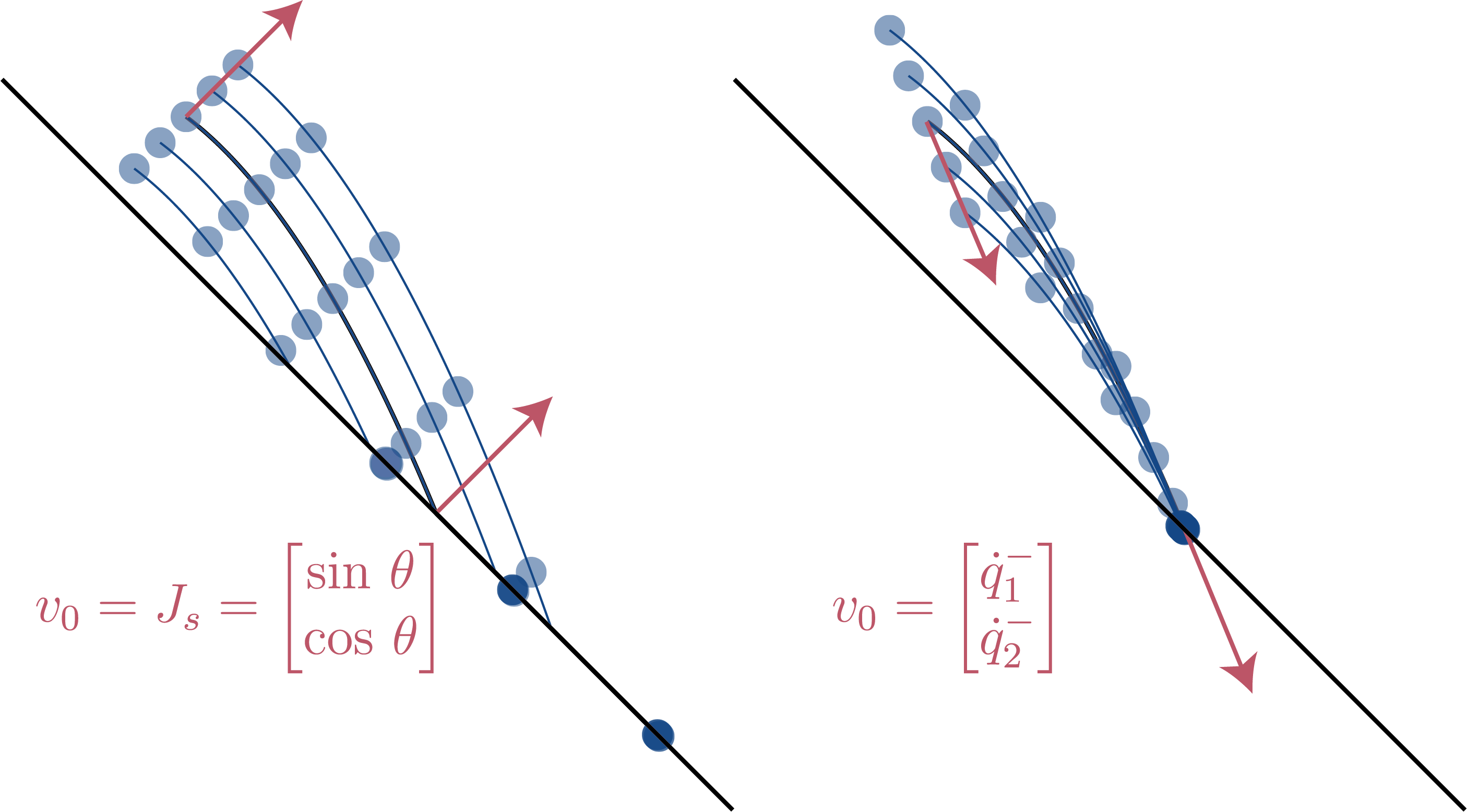
Figure 7: Ball drop example with sliding friction (left) and sticking friction (right). In sliding, position variations in the direction of the constraint are eliminated. $v_{0}$ is the eigenvector associated with the zero eigenvalue and $\theta$ is the angle of the surface. In sticking, position variations in the direction of pre-impact velocity are eliminated. $q_{1}$ is the horizontal configuration, and $q_{2}$ is the vertical configuration.

For plastic impact into sticking, $\mathrm{U},\mathrm{C})$, variations in configuration map differently than velocity variations. This is because the tangential constraint is only applied to the velocity and not the position (i.e. it is non-holonomic), whereas in the normal direction, both position and velocity are constrained. The sticking saltation matrix $\Xi{(\mathrm{U},\mathrm{C})}$ reflects this change, where there is no longer a repeated element in the block diagonal. Instead, the only nonzero component is how variations in position map onto the constraint surface (57)–(58). The velocity components are all zero because velocity is fully constrained to zero. Again, we analyze the non-zero block by computing the eigenvalues and corresponding eigenvectors:

$$\lambda_{0} =0, \lambda_{1} =1$$

$$v_{0} =\begin{bmatrix}\dot{q}_{1}\\ \dot{q}_{2}\end{bmatrix}, v_{1} =\begin{bmatrix}-\cos{(\theta)}\\ \sin{(\theta)}\end{bmatrix}$$ (60)

Similar to the sliding case, variations tangential to the constraint are preserved. However, the zero eigenvector is different. Configuration variations that are in the same direction as the impact velocity disappear. Fig. 7 illustrates this idea, where position variations in the direction of the pre-impact velocity are eliminated. This is intuitive because the ball impacting earlier or later has no effect if the variation is in line with the impact velocity, it will hit the same contact point and stick.

V Saltation matrices for generalized rigid body systems with unilateral constraints

For rigid body systems with contacts, the hybrid modes are the enumeration of different contact conditions. This section defines the dynamics of these systems and calculates the saltation matrix of all the common mode transitions for a single constraint. This section generalizes much of the intuition developed in Sec. IV.

V-A Dynamics derivation

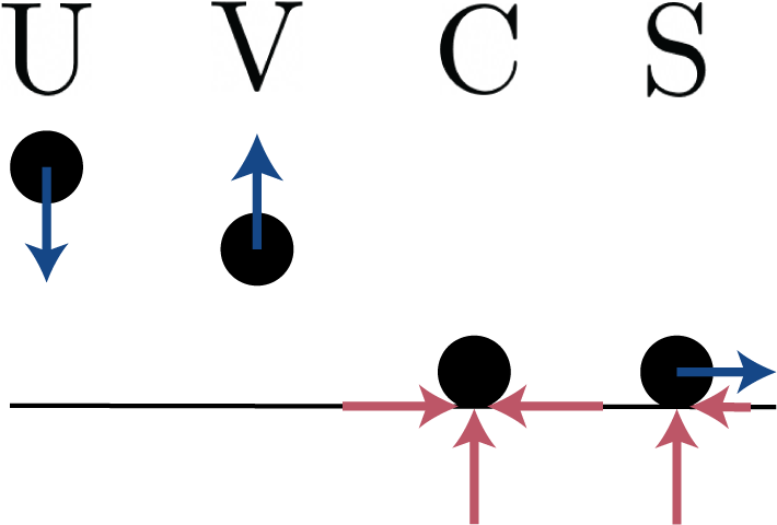
Figure 8: Depicting the different rigid body hybrid modes considered where blue arrows depict velocities and red arrows depict forces. $\mathrm{U}$ is the unconstrained mode with approaching velocity to the constraint, $\mathrm{V}$ is the unconstrained mode with separating velocity, $\mathrm{C}$ is the constrained mode, and $\mathrm{S}$ is the sliding mode on the constraint. A single planar point is shown here, but the system may have additional degrees of freedom.

The following examples consider four modes, illustrated in Fig. 8: the unconstrained mode approaching the constraint surface to be $\mathrm{U}$, the unconstrained mode leaving the surface $\mathrm{V}$, a constrained mode $\mathrm{C}$, and a sliding with friction mode $\mathrm{S}$. The reason both $\mathrm{U}$ and $\mathrm{V}$ are included is to ensure that elastic impact is not defined with a self-reset and to avoid degenerate impacts just after liftoff, when the velocity is not approaching the constraint but the guard condition is satisfied $g_{\mathrm{n}}\leq 0$, especially when using numerical integration.

The states of the system are the configuration coordinates $q$ and their velocities $\dot{q}$, such that $x:=[q,\dot{q}]^{T}$. The dimension of the configuration $q$ is defined to be $m$, while the dimension of the state space $x$ is $n=2m$. Contacts between rigid bodies are regulated through a unilateral constraint in the normal (n) direction, $g_{\mathrm{n}}(t,x)\geq 0$. Note that $g_{\mathrm{n}}(t,x)$ only depends on the configuration $q$ and not the velocity. When rigid bodies are in contact they must satisfy $g_{\mathrm{n}}(t,x)=0$.

The Jacobian of $g_{\mathrm{n}}$ with respect to the configuration coordinates is defined to be $J_{\mathrm{n}}:=\mathrm{D}_{q}g_{\mathrm{n}}(t,x)$. In the sliding mode, the constraint Jacobian consists of just this normal direction constraint, $J_{\mathrm{S}}=J_{\mathrm{n}}$. However, if the no slip condition is added, the constrained mode C has a constraint Jacobian of:

$$J_{\mathrm{C}}=\begin{bmatrix}J_{\mathrm{n}}\\ J_{\mathrm{t}}\end{bmatrix}$$ (61)

where $J_{\mathrm{t}}$ is the tangential velocity constraint Jacobian. For unconstrained modes, $J$ is empty.

In any mode, the following acceleration constraint is applied based on $J$ for that mode to maintain the active constraints until the next guard:

$$J(t,x)\ddot{q}+\dot{J}(t,x)\dot{q}=0$$ (62)

The equations of motion for each mode are defined by the constrained manipulator dynamics, e.g. [124], where this constraint is combined with Lagrangian dynamics:

$$\begin{bmatrix}M&J^{T}\\ J&0\end{bmatrix}\begin{bmatrix}\ddot{q}\\ f\end{bmatrix}=\begin{bmatrix}\Upsilon-N\\ 0\end{bmatrix}-\begin{bmatrix}C\\ \dot{J}\end{bmatrix}\dot{q}$$ (63)

[125, Eqn. 33] where $f$ is the constraint force vector (Lagrange multiplier), $M(q)$ is the mass matrix, $C(q,\dot{q})$ is the Coriolis matrix, $\Upsilon(u)$ the input vector, and $N(q,\dot{q})$ are the other nonlinear forces such as gravity and sliding friction.

To help with the following equations, the $\dagger$ notation from [4, Eqn. 8] is adopted here, where in each mode:

$$\begin{bmatrix}M^{\dagger}&J^{\dagger T}\\ J^{\dagger}&\Lambda^{\dagger}\\ \end{bmatrix}:=\begin{bmatrix}M&J^{T}\\ J&0\end{bmatrix}^{-1}$$ (64)

This definition produces a number of identities, in particular:

$$M^{\dagger}M=I_{m\times m}-J^{\dagger T}J$$ (65)

[4, Eqn. 11], which will be helpful in simplifying the saltation matrix expressions.

With this notation the state space dynamics can be expressed as:

$$\dot{x}=\frac{d}{dt}\begin{bmatrix}q\\ \dot{q}\end{bmatrix}=\begin{bmatrix}\dot{q}\\ M^{\dagger}\left(\Upsilon-N-C\dot{q}\right)-J^{\dagger T}\dot{J}\dot{q}\end{bmatrix}$$ (66)

[4, Eqn. 75] where each $\dagger$ component is different depending on the hybrid mode based on $J$. For the unconstrained case, $M^{\dagger}=M^{-1}$.

Similarly, the constraint forces $f(t,x)$ are calculated from the bottom row of (63):

$$f(t,x)=J^{\dagger}\left(\Upsilon-N-C\dot{q}\right)-\Lambda^{\dagger}\dot{J}\dot{q}$$ (67)

Coulomb friction is used in the sliding mode – frictional forces in the tangential direction $f_{\mathrm{t}}$ (included in $N$) are applied to resist sliding motion proportional to the normal constraint force, $f_{\mathrm{n}}$, and in the direction resisting the sliding velocity, $v_{\mathrm{t}}=J_{\mathrm{t}}\dot{q}$:

$$f_{\mathrm{t}}=\mu_{k}\|f_{\mathrm{n}}\|\frac{J_{\mathrm{t}}\dot{q}}{\|J_{\mathrm{t}}\dot{q}\|}=\mu_{k}\|f_{\mathrm{n}}\|\frac{v_{\mathrm{t}}}{\|v_{\mathrm{t}}\|}$$ (68)

where $\mu_{k}$ is the kinetic coefficient of friction.

When a contact constraint is added, for example the normal surface constraint $g_{\mathrm{n}}$, an impact law $J_{\mathrm{n}}\dot{q}^{+}=-eJ_{\mathrm{n}}\dot{q}^{-}$ is applied (where the coefficient of restitution $e=1$ is perfectly elastic and $e=0$ is perfectly plastic) along with the impulse momentum equation to get:

$$\begin{bmatrix}\dot{q}^{+}\\ \hat{p}\end{bmatrix}=\begin{bmatrix}M&J_{\mathrm{n}}^{T}\\ J_{\mathrm{n}}&0\end{bmatrix}^{-1}\!\!\begin{bmatrix}M\\ -eJ_{\mathrm{n}}\end{bmatrix}\dot{q}^{-}=\begin{bmatrix}M^{\dagger}_{\mathrm{n}}&J^{\dagger T}_{\mathrm{n}}\\ J^{\dagger}_{\mathrm{n}}&\Lambda_{\mathrm{n}}^{\dagger}\\ \end{bmatrix}\!\!\begin{bmatrix}M\\ -eJ_{\mathrm{n}}\end{bmatrix}\dot{q}^{-}$$ (69)

[4, Eqn. 23], [126], where $\hat{p}$ is the impulse magnitude vector. Since the positions do not change instantaneously, the state space reset map for elastic, frictionless impact from mode U to mode V is:

$$x^{+}=\begin{bmatrix}q^{+}\\ \dot{q}^{+}\end{bmatrix}=R_{(\mathrm{U,V})}(t,x^{-})=\begin{bmatrix}q^{-}\\ M^{\dagger}_{\mathrm{n}}M\dot{q}^{-}-eJ^{\dagger T}_{\mathrm{n}}J_{\mathrm{n}}\dot{q}^{-}\end{bmatrix}$$ (70)

The plastic, frictionless impact reset map into mode S follows (70) but with $e=0$ (and written with $M^{\dagger}_{\mathrm{S}}$ for mode S, though $M^{\dagger}_{\mathrm{S}}=M^{\dagger}_{\mathrm{n}}$ since $J_{\mathrm{S}}=J_{\mathrm{n}}$):

$$x^{+}=\begin{bmatrix}q^{+}\\ \dot{q}^{+}\end{bmatrix}=R_{(\mathrm{U},\mathrm{S})}(t,x^{-})=\begin{bmatrix}q^{-}\\ M^{\dagger}_{\mathrm{S}}M\dot{q}^{-}\end{bmatrix}$$ (71)

The frictional, plastic impact reset map, $R_{(\mathrm{U},\mathrm{C})}$, follows (71) but with $J_{\mathrm{C}}$ and $M^{\dagger}_{\mathrm{C}}$ instead of $J_{\mathrm{S}}$ and $M^{\dagger}_{\mathrm{S}}$. Similarly, the liftoff reset maps into modes U or V are the same except that there is no constraint $J$, and so the reset simplifies to an identity map. Note that the reset map does not depend on the prior mode, so for example $R_{(\mathrm{S,C})}=R_{(\mathrm{U},\mathrm{C})}$.

V-B Apex

Apex is a “virtual” hybrid event – one that does not have a physical reset map or change in the dynamics – and is triggered when the velocity switches from going away from the constraint to towards the constraint $(\mathrm{V,U})$. As the reset map is identity, and the dynamics match before and after (since there is not a difference in control at this event) the saltation matrix is identity following (14):

$$\Xi_{(\mathrm{V,U})}=I_{n\times n}$$ (72)

V-C Liftoff

Liftoff is a hybrid transition into mode $\mathrm{V}$ from $\mathrm{S}$ or $\mathrm{C}$ that depends on the constraint force $f(t,x)$, (67), which is a function of both time and state (and implicitly a function of control input). The guard for liftoff is determined by $f_{\mathrm{n}}$, the constraint force in the $J_{\mathrm{n}}$ direction – if the force becomes non-repulsive, then the contact is released:

$$g_{(\mathrm{C,V})}(t,x)=f_{\mathrm{n}}(t,x)$$ (73)

$$g_{(\mathrm{S,V})}(t,x)=f_{\mathrm{n}}(t,x)$$ (74)

Because the hybrid event occurs when the constraint force goes to zero, the dynamics at the boundary are equal. This is true even in the case of sticking friction in mode $\mathrm{C}$, as the friction cone ensures that either the system transitions to sliding mode $\mathrm{S}$ (as discussed in Sec. V-F) or the frictional force goes to zero at the same time. The state does not jump during liftoff, which meaning the reset map for liftoff is an identity transformation. Since both conditions of (14) are met for liftoff, the saltation matrices are identity:

$$\Xi_{(\mathrm{C,V})} =I_{n\times n}$$ (75)

$$\Xi_{(\mathrm{S,V})} =I_{n\times n}$$ (76)

Due to the smooth nature of liftoff, these events can be safely ignored when considering variations from liftoff.

V-D Plastic impact

Plastic impact occurs when the unconstrained mode $\mathrm{U}$ makes contact and transitions to either the sliding mode $\mathrm{S}$ or the constrained mode $\mathrm{C}$. First, consider plastic impact into sliding $(\mathrm{U},\mathrm{S})$. For simplicity, frictionless sliding $\mu_{k}=0$ is assumed to expose the structure in the saltation matrix, but the same calculations can be made with non-zero sliding friction $\mu_{k}>0$. The dynamics for each mode is from (66):

$$F_{\mathrm{U}}(t,x^{-}) =\begin{bmatrix}\dot{q}^{-}\\ M^{-1}(\Upsilon-C^{-}\dot{q}^{-}-N)\end{bmatrix}$$ (77)

$$F_{\mathrm{S}}(t,x^{+}) =\begin{bmatrix}\dot{q}^{+}\\ M_{\mathrm{S}}^{\dagger}(\Upsilon-C^{+}\dot{q}^{+}-N)-J_{\mathrm{S}}^{\dagger T}\dot{J}_{\mathrm{S}}^{+}\dot{q}^{+}\end{bmatrix}$$ (78)

Note that $-$ or $+$ on $\mathrm{C}$ and $\dot{J}$ indicates that these functions use the pre- or post-impact velocity, $\dot{q}^{-}$ or $\dot{q}^{+}$, respectively. The Jacobian of the reset map for plastic impact, (71), is:

$$\mathrm{D}_{x}R_{(\mathrm{U},\mathrm{S})}(t,x^{-})=\begin{bmatrix}I_{m\times m}&0_{m\times m}\\ \mathrm{D}_{q}(M_{\mathrm{S}}^{\dagger}M\dot{q}^{-})&M_{\mathrm{S}}^{\dagger}M\end{bmatrix}$$ (79)

The Jacobian of the guard $\mathrm{D}_{x}g_{(\mathrm{U},\mathrm{S})}(t,x^{-})$ is:

$$\mathrm{D}_{x}g_{(\mathrm{U},\mathrm{S})}(t,x^{-}) =\begin{bmatrix}J_{\mathrm{S}}&0_{1\times m}\end{bmatrix}$$ (80)

while the denominator of $\Xi_{(\mathrm{U},\mathrm{S})}$ is the impact velocity:

$$\mathrm{D}_{x}g_{(\mathrm{U},\mathrm{S})}(t,x^{-})F_{\mathrm{U}}(t,x^{-}) =\begin{bmatrix}J_{\mathrm{S}}&\!0_{1\times m}\end{bmatrix}F_{\mathrm{U}}(t,x^{-})=J_{\mathrm{S}}\dot{q}^{-}$$ (81)

In this example, the guard and reset map are independent of time, $\mathrm{D}_{t}R=0_{n\times 1},\mathrm{D}_{t}g=0$. However, in other cases such as a paddle juggler [127], the impact surface can move as a function determined by time, in which case the guard and reset would depend on the prescribed motion.

To further simplify the component of the saltation matrix (2) that contains the difference between dynamics, $F_{\mathrm{S}}-\mathrm{D}_{x}RF_{\mathrm{U}}$, the following steps are applied. First, substitute in $\dot{q}^{+}=M_{\mathrm{S}}^{\dagger}M\dot{q}^{-}=\dot{q}^{-}-J_{\mathrm{S}}^{\dagger T}J_{\mathrm{S}}\dot{q}^{-}$ using the reset map (71) and the identity (65). Then, plugging into the difference between dynamics:

$$F_{\mathrm{S}}(t,x^{+})-\mathrm{D}_{x}R_{(\mathrm{U},\mathrm{S})}(t,x^{-})F_{\mathrm{U}}(t,x^{-})=$$ (82)

$$\begin{bmatrix}-J_{\mathrm{S}}^{\dagger T}J_{\mathrm{S}}\dot{q}^{-}\\ M_{\mathrm{S}}^{\dagger}(C^{-}\dot{q}^{-}-C^{+}\dot{q}^{+})-J_{\mathrm{S}}^{\dagger T}\dot{J}_{\mathrm{S}}^{+}\dot{q}^{+}-\mathrm{D}_{q}(M_{\mathrm{S}}^{\dagger}M\dot{q}^{-})\dot{q}^{-}\end{bmatrix}$$ (83)

The saltation matrix for plastic impact is obtained by inserting all terms into (2) and simplifying (using (65) again):

$$\Xi_{(\mathrm{U},\mathrm{S})} =\begin{bmatrix}M_{\mathrm{S}}^{\dagger}M&0_{m\times m}\\ Z_{\mathrm{S}}+\mathrm{D}_{q}(M_{\mathrm{S}}^{\dagger}M\dot{q}^{-})&M_{\mathrm{S}}^{\dagger}M\end{bmatrix}$$ (84)

where:

$$Z_{\mathrm{S}}=\left(M_{\mathrm{S}}^{\dagger}(C^{-}\dot{q}^{-}-C^{+}\dot{q}^{+})-J_{\mathrm{S}}^{\dagger T}\dot{J}_{\mathrm{S}}^{+}\dot{q}^{+}-\mathrm{D}_{q}(M_{\mathrm{S}}^{\dagger}M\dot{q}^{-})\dot{q}^{-}\right)J_{\mathrm{S}}/(J_{\mathrm{S}}\dot{q}^{-})$$ (85)

Note that the difference between the Jacobian of the reset map $\mathrm{D}_{x}R$, (79), is in the first column of the matrix where the identity matrix is now $M_{\mathrm{S}}^{\dagger}M$ and the element on the lower left differs by the term in (85).

When impacting into the frictional constrained mode $\mathrm{C}$, all steps remain the same except with $J_{\mathrm{C}}$ instead of $J_{\mathrm{S}}$ (and similarly $M^{\dagger}_{\mathrm{C}}$ and $J^{\dagger T}_{\mathrm{C}}$). However, the upper left block of the saltation matrix no longer simplifies as nicely with the Jacobian of the guard $\mathrm{D}_{x}g$ terms. This is because $J_{\mathrm{S}}=\mathrm{D}_{x}g=J_{\mathrm{n}}$ but $J_{\mathrm{C}}\neq\mathrm{D}_{x}g$. Rather, $\mathrm{D}_{x}g=J_{\mathrm{n}}$ is a row of $J_{\mathrm{C}}$, i.e. the non-penetrating constraint. The resulting saltation matrix is:

$$\Xi_{(\mathrm{U},\mathrm{C})} =\begin{bmatrix}I_{m\times m}-\frac{J_{\mathrm{C}}^{\dagger T}J_{\mathrm{C}}\dot{q}^{-}J_{\mathrm{n}}}{J_{\mathrm{n}}\dot{q}^{-}}&0_{m\times m}\\ Z_{\mathrm{C}}+\mathrm{D}_{q}(M_{\mathrm{C}}^{\dagger}M\dot{q}^{-})&M_{\mathrm{C}}^{\dagger}M\end{bmatrix}$$ (86)

where:

$$Z_{\mathrm{C}}=\left(M_{\mathrm{C}}^{\dagger}(C^{-}\dot{q}^{-}-C^{+}\dot{q}^{+})-J_{\mathrm{C}}^{\dagger T}\dot{J}_{\mathrm{C}}^{+}\dot{q}^{+}-\mathrm{D}_{q}(M_{\mathrm{C}}^{\dagger}M\dot{q}^{-})\dot{q}^{-}\right)J_{\mathrm{C}}/(J_{\mathrm{C}}\dot{q}^{-})$$ (87)

Again, the difference between the saltation matrix and the Jacobian of the reset is in the left column associated with the configuration variations. However, the upper left block no longer maps configuration variations exactly the same as velocity variations in the lower right, because the tangential constraint is only a velocity constraint – the contact point can be anywhere on the contact surface, whereas the velocity of the contact point must be the same everywhere on the surface.

Other than the upper left block, the structure of $(\mathrm{U},\mathrm{S})$ and $(\mathrm{U},\mathrm{C})$ saltation matrices look remarkably similar, with the interchange of $J_{\mathrm{S}}$ and $J_{\mathrm{C}}$ being the only other difference. In the example in Sec. IV, the lower left block of these saltation matrices was zero. This block is comprised of Coriolis-like terms, so for simple systems like the ball drop, Coriolis terms do not exist in the dynamics and the lower left block of the saltation matrix collapses to zero. However, for systems of appreciable complexity, this does not hold.

V-E Elastic impact

When the coefficient of restitution is non-zero, states in the approaching unconstrained mode $\mathrm{U}$ transition directly to the separating unconstrained mode $\mathrm{V}$ through elastic impact. The dynamics for each mode, (66), are:

$$F_{\mathrm{U}}(t,x^{-}) =\begin{bmatrix}\dot{q}\\ M^{-1}(\Upsilon-C^{-}\dot{q}^{-}-N)\end{bmatrix}$$ (88)

$$F_{\mathrm{V}}(t,x^{+}) =\begin{bmatrix}\dot{q}^{+}\\ M^{-1}(\Upsilon-C^{+}\dot{q}^{+}-N)\end{bmatrix}$$ (89)

Again, note that $-$ or $+$ on $\mathrm{C}$ indicates that these functions use the pre- or post-impact velocity, $\dot{q}^{-}$ or $\dot{q}^{+}$, respectively. The Jacobian of the reset map for elastic impact, (70), is:

$$\mathrm{D}_{x}R_{({\mathrm{U,V}})}^{-}=\begin{bmatrix}I_{m\times m}&0_{m\times m}\\ \!\mathrm{D}_{q}(\!(M^{\dagger}_{\mathrm{n}}M-eJ^{\dagger T}_{\mathrm{n}}J_{\mathrm{n}})\dot{q}^{-})&M^{\dagger}_{\mathrm{n}}M-eJ^{\dagger T}_{\mathrm{n}}J_{\mathrm{n}}\!\end{bmatrix}$$ (90)

The Jacobian of the guard is again $\mathrm{D}_{x}g=[J_{\mathrm{n}},0_{1\times n}]$. Plugging each component back into the full saltation matrix equation results in:

$$\Xi_{(\mathrm{U,V})}\! =\!\begin{bmatrix}M^{\dagger}M-eJ^{\dagger T}J&0_{m\times m}\\ \!Z_{\mathrm{V}}\!+\!\mathrm{D}_{q}(\!(M^{\dagger}M-eJ^{\dagger T}J)\dot{q}^{-})&\!\!\!M^{\dagger}M\!-\!eJ^{\dagger T}\!J\!\end{bmatrix}$$ (91)

where $J$ and $M^{\dagger}$ use the normal constraint, $J_{\mathrm{n}}$ and $M^{\dagger}_{\mathrm{n}}$, and:

$$Z_{\mathrm{V}}=\left(\left[M^{-1}(C^{-}-C^{+}(M^{\dagger}_{\mathrm{n}}M-eJ^{\dagger T}_{\mathrm{n}}J_{\mathrm{n}}))-\mathrm{D}_{q}((M^{\dagger}_{\mathrm{n}}M-eJ^{\dagger T}_{\mathrm{n}}J_{\mathrm{n}})\dot{q}^{-})\right]\dot{q}^{-}+(1+e)J^{\dagger T}_{\mathrm{n}}J_{\mathrm{n}}M^{-1}(\Upsilon-C^{-}\dot{q}^{-}-N)\right)J_{\mathrm{n}}/(J_{\mathrm{n}}\dot{q}^{-})$$ (92)

Note that the following substitution can be made $M^{\dagger}M-eJ^{\dagger T}J=I_{m\times m}-(1+e)J^{\dagger T}J$ by (65).

V-F Stick-slip friction

The saltation matrix for stick-slip friction has been calculated in [10, Sec. 7.3]. This section computes this saltation matrix for a generalized system and analyzes its components.

When the friction cone is broken, the mode is switched from the constrained mode $\mathrm{C}$ to the sliding mode $\mathrm{S}$. The guard to check for slipping is the friction cone:

$$g_{(\mathrm{C,S})}(t,x)=\mu_{s}\|f_{\mathrm{n}}(t,x)\|-\|f_{\mathrm{t}}(t,x)\|=0$$ (93)

where $\mu_{s}$ is the coefficient of static friction. The reset map for these hybrid transitions is an identity transformation $x^{+}=R_{(\mathrm{C,S})}(x^{-})=x^{-}$, and therefore $\mathrm{D}_{x}R_{(\mathrm{C,S})}=I_{n\times n}$.

If the guard $g_{(\mathrm{C,S})}$ is met, it can be assumed that slipping will also occur in the direction of the maximum tangential force. Therefore, at the slipping boundary, if both the coefficient of static friction and kinetic friction match, $\mu_{s}=\mu_{k}$, then $\Delta F=0$ (as the frictional force reaches and then maintains the value in (68)) and the saltation matrix is identity by (14). Indeed, any friction model (not just Coulomb) where the frictional force matches at the boundary results in an identity saltation matrix. This includes models where $\mu_{k}$ is a function of velocity, such as Stribeck friction, so long as at $\|v_{\mathrm{t}}\|=\|J_{\mathrm{t}}\dot{q}\|=0$, $\mu_{k}(0)=\mu_{s}$, to get:

$$\mu_{s}=\mu_{k}\implies F_{\mathrm{S}}=F_{\mathrm{C}}$$ (94)

$$\implies\Xi_{(\mathrm{C,S})} =I_{n\times n}$$ (95)

If $\mu_{s}\neq\mu_{k}$, the saltation matrix is not necessarily identity, and the general computations of the saltation matrix can be made to obtain this form:

$$\mu_{s}\neq\mu_{k}\implies F_{\mathrm{S}}^{+}\neq F_{\mathrm{C}}^{-}$$ (96)

$$\implies\Xi_{(\mathrm{C,S})} =I_{n\times n}+\frac{(F_{\mathrm{S}}^{+}-F_{\mathrm{C}}^{-})\mathrm{D}_{x}g_{(\mathrm{C,S})}}{\mathrm{D}_{t}g_{(\mathrm{C,S})}+\mathrm{D}_{x}g_{(\mathrm{C,S})}F_{\mathrm{C}}^{-}}$$ (97)

For this saltation matrix, position variations do not change because the reset map is identity and the top row of $F_{\mathrm{S}}$ and $F_{\mathrm{C}}$ are equal (i.e. the velocity $\dot{q}$ does not change between modes).

However, this saltation matrix will be very prone to modeling errors as it depends on knowing exactly how the sliding and sticking coefficients differ. From a modeling perspective, it may be advantageous to assume that at the boundaries the sliding and sticking coefficients match.

V-G Slip-stick friction

When the tangential velocity in mode $\mathrm{S}$ goes to zero, the sliding stops and “sticks” into the constrained mode $\mathrm{C}$. Therefore, the guard at slip-stick friction is just the magnitude of the tangential velocity:

$$g_{(\mathrm{S,C})}(t,x) =\|J_{\mathrm{t}}\dot{q}\|=\|v_{\mathrm{t}}\|$$ (98)

$$\mathrm{D}_{x}g_{(\mathrm{S,C})}(t,x) =\begin{bmatrix}\dot{J}_{\mathrm{t}}^{-}&J_{\mathrm{t}}\end{bmatrix}$$ (99)

The guard also has the condition $\|f_{\mathrm{t}}\|<\mu_{s}\|f_{\mathrm{n}}\|$. However, note that the way tangential friction forces are calculated is different in the sliding mode $\mathrm{S}$ than in the sticking mode $\mathrm{C}$. In sliding, the tangential force is proportional to the normal force, $\|f_{\mathrm{t}}\|=\mu_{k}\|f_{\mathrm{n}}\|$, (68). In the constrained sticking mode, the force vector is calculated from Lagrange multipliers as in (67). These generally are not equal and so there is a difference in the tangential force at the transition, and thus a difference in dynamics.

The reset is an identity transformation, $x^{+}=R_{(\mathrm{S,C})}(x^{-})=x^{-}$, and therefore $\mathrm{D}_{x}R_{(\mathrm{S,C})}=I_{n\times n}$, so the saltation matrix is primarily composed of the difference between the dynamics of both modes and the tangential velocity term from the guard. Since the guard is not directly a function of time or control input in this case, $\mathrm{D}_{t}g_{(\mathrm{S,C})}=0$ and can be ignored, and the saltation matrix is:

$$\Xi_{(\mathrm{S,C})}=I_{n\times n}+\frac{(F_{\mathrm{C}}^{+}-F_{\mathrm{S}}^{-})\begin{bmatrix}\dot{J}_{\mathrm{t}}^{-}&J_{\mathrm{t}}\end{bmatrix}}{\dot{J}_{\mathrm{t}}^{-}\dot{q}^{-}+J_{\mathrm{t}}\ddot{q}^{-}}$$ (100)

Note that the denominator is the tangential acceleration constraint (62) in mode $\mathrm{C}$. If this condition is met at the exact moment that the velocity guard is satisfied while in the sliding mode $\mathrm{S}$, the saltation matrix is not well defined; however, this would violate the transversality assumption (11). For this saltation matrix, as with stick-slip, position variations do not change because the reset map is identity and the top row of $F_{\mathrm{C}}$ and $F_{\mathrm{S}}$ are equal (i.e. the velocity $\dot{q}$ does not change between modes).

V-H Analysis of Saltation Matrices for Rigid Bodies

This section presents saltation matrix derivations for a number of hybrid transitions that occur in rigid body systems with contact, as summarized in Table II. These derivations reveal patterns among many of these saltation matrices. For instance, the upper right block of the saltation matrix is zero for every case presented here. This is due to the second order nature of mechanical systems as a whole (i.e. acceleration is the derivative of velocity, which is the derivative of position). This makes it convenient to perform the eigen-analysis as in Sec. IV. The eigenvalues and eigenvectors of a block triangular matrix are the eigenvalues and eigenvectors of its diagonal block components, and the lower left block does not affect them. In applications where only the eigenvalues of the saltation matrix of interest, knowing the structure of the saltation matrix means the full saltation matrix need not be computed.

Four of the saltation matrices analyzed are identity: apex (72), the two liftoff cases (75,76), and stick-slip under constant friction coefficient (95). This occurs when the reset map is identity and the dynamics in each mode are equivalent, as in (14). Outside of these identity cases, the stick-slip with unequal friction coefficients (97) and slip-stick (100) transitions also have an identity reset map because there is no instantaneous change in positions or velocities. An identity reset map allows for further insight into the eigen-properties of these matrices. Both of these saltation matrices can be written as $\Xi=I_{n\times n}+ab^{T}$ where $a$ and $b$ are $n\times 1$ vectors and $ab^{T}$ is their outer product. The eigenvalues of a matrix with this structure are all $1$ except for one eigenvalue of $1+a^{T}b$ with corresponding eigenvector $a$. This can be easily shown from the equality:

$$(I+ab^{T})a =a+a(b^{T}a)=(1+a^{T}b)a$$ (101)

This makes it possible to compute the eignvalues of these saltation matrices without performing the full matrix computation.

Two non-identity saltation matrices had equivalent diagonal blocks, sliding plastic impact (84) and elastic impact (91). This occurs because the guard surface enforces an equivalent constraint on both position and velocities to be along the guard. When a non-holonomic constraint is added in mode $\mathrm{C}$, this equivalency breaks. Equal diagonal blocks means that the eigenvalues of these saltation matrices are the eigenvalues of a diagonal block repeated twice. Table II summarizes the properties of identity reset map, matching hybrid dynamics, equal diagonal blocks, as well as equation number for each saltation matrix.

TABLE II: Properties of Saltation Matirx for Different Rigid Body Mode Transitions

Transition	$R=I$	$F^{+}=F^{-}$	Equal Diag. Blocks	Eq. #
$(\mathrm{V},\mathrm{U})$	✓	✓	✓	(72)
$(\mathrm{C},\mathrm{V})$	✓	✓	✓	(75)
$(\mathrm{S},\mathrm{V})$	✓	✓	✓	(76)
$(\mathrm{U},\mathrm{S})$	✗	✗	✓	(84)
$(\mathrm{U},\mathrm{C})$	✗	✗	✗	(86)
$(\mathrm{U},\mathrm{V})$	✗	✗	✓	(91)
$(\mathrm{C},\mathrm{S})$	✓	if $\mu_{s}=\mu_{k}$	if $\mu_{s}=\mu_{k}$	(95,97)
$(\mathrm{S},\mathrm{C})$	✓	✗	✗	(100)

VI Conclusion

The saltation matrix is an essential tool when dealing with hybrid systems with state dependent switches. This paper presents a derivation of the saltation matrix with two different methods and demonstrates how the saltation matrix can be used in linear and quadratic forms for hybrid systems. A survey of where saltation matrices are used in other fields is also presented. In the past, it has been heavily utilized for analyzing the stability of periodic systems, but more recently it has been critical for analyzing and designing non-periodic behaviors. This analysis is especially useful for robotics where many important robotic motions are not periodic, but are hybrid due to the discontinuous nature of impact in rigid body systems with unilateral constraints.

To further explore the nature of contact and how variations are mapped through them, a simple contact system is considered to compute the saltation matrix for plastic impact and analyze the different components of the resulting saltation matrices. These saltation matrices capture how position variations are mapped through contact, whereas the Jacobian of the reset map does not provide any information on position. In addition to this simple example, saltation matrices are computed for each of the hybrid transitions for a generalized rigid body model and we give insights on their structure. These computations are especially useful because the rigid body model covers a wide variety of systems and will help when getting started using saltation matrices for these systems. Saltation matrices exhibit common structures that can be exploited. In particular, by only using the Jacobian of the reset map instead of the saltation matrix, the entirety of the position variational information is lost. For other hybrid transitions such as stick-slip friction, the Jacobian of the reset map provides no additional information because it is an identity transformation and all the information is contained in the saltation matrix.

By using saltation matrices for hybrid systems, efficient analysis, planning, control, and state estimation algorithms can be produced. This is especially important as hybrid systems naturally have combinatoric time complexities and through the use of these tools we can simplify these problems. The hope of this paper is to introduce the topic of saltation matrices to a broader community so that we can, as a whole, develop better methods for dealing with the complexities of hybrid systems and their applications.

References

- [1] A. Back, J. M. Guckenheimer, and M. Myers, “A dynamical simulation facility for hybrid systems,” in Hybrid Systems, ser. Lecture Notes in Computer Science. Springer Berlin / Heidelberg, 1993, vol. 736.
- [2] J. Lygeros, K. H. Johansson, S. N. Simic et al., “Dynamical properties of hybrid automata,” IEEE Transactions on Automatic Control, vol. 48, no. 1, pp. 2–17, 2003.
- [3] R. Goebel, R. G. Sanfelice, and A. R. Teel, “Hybrid dynamical systems,” IEEE Control Systems Magazine, vol. 29, no. 2, pp. 28–93, 2009.
- [4] A. M. Johnson, S. A. Burden, and D. E. Koditschek, “A hybrid systems model for simple manipulation and self-manipulation systems,” The International Journal of Robotics Research, vol. 35, no. 11, 2016.
- [5] W. Yang and M. Posa, “Impact invariant control with applications to bipedal locomotion,” in IEEE/RSJ International Conference on Intelligent Robots and Systems, 2021, pp. 5151–5158.
- [6] G. Council, S. Yang, and S. Revzen, “Deadbeat control with (almost) no sensing in a hybrid model of legged locomotion,” in International Conference on Advanced Mechatronic Systems, 2014, pp. 475–480.
- [7] M. H. Raibert, H. B. Brown Jr, M. Chepponis et al., “Dynamically stable legged locomotion,” Massachusetts Inst of Tech Cambridge Artificial Intelligence Lab, Tech. Rep., 1989.
- [8] M. Aizerman and F. Gantmakher, “On the stability of periodic motions,” Journal of Applied Mathematics and Mechanics, vol. 22, no. 6, pp. 1065–1078, 1958.
- [9] A. F. Filippov, Differential Equations with Discontinuous Righthand Sides. Springer, 1988.
- [10] R. Leine and H. Nijmeijer, Dynamics and Bifurcations of Non-Smooth Mechanical Systems. Springer, 2004.
- [11] A. P. Ivanov, “The stability of periodic solutions of discontinuous systems that intersect several surfaces of discontinuity,” Journal of Applied Mathematics and Mechanics, vol. 62, no. 5, pp. 677–685, 1998.
- [12] N. J. Kong, J. J. Payne, G. Council, and A. M. Johnson, “The Salted Kalman Filter: Kalman filtering on hybrid dynamical systems,” Automatica, vol. 131, p. 109752, 2021.
- [13] N. J. Kong, G. Council, and A. M. Johnson, “iLQR for piecewise-smooth hybrid dynamical systems,” in IEEE Conference on Decision and Control, December 2021, pp. 5374–5381.
- [14] N. Kong, C. Li, and A. M. Johnson, “Hybrid iLQR model predictive control for contact implicit stabilization on legged robots,” arXiv:2207.04591 [cs.RO], 2022.
- [15] J. J. Payne, N. J. Kong, and A. M. Johnson, “The uncertainty aware Salted Kalman Filter: State estimation for hybrid systems with uncertain guards,” in IEEE/RSJ Intl. Conference on Intelligent Robots and Systems, October 2022.
- [16] J. Zhu, N. J. Kong, G. Council, and A. M. Johnson, “Hybrid event shaping to stabilize periodic hybrid orbits,” in IEEE Intl. Conference on Robotics and Automation, Philadelphia, PA, May 2022, pp. 6600–6606.
- [17] M. Rijnen, A. Saccon, and H. Nijmeijer, “On optimal trajectory tracking for mechanical systems with unilateral constraints,” in IEEE Conference on Decision and Control, 2015, pp. 2561–2566.
- [18] M. Rijnen, J. B. Biemond, N. Van De Wouw et al., “Hybrid systems with state-triggered jumps: Sensitivity-based stability analysis with application to trajectory tracking,” IEEE Transactions on Automatic Control, vol. 65, no. 11, pp. 4568–4583, 2019.
- [19] A. Saccon, N. van de Wouw, and H. Nijmeijer, “Sensitivity analysis of hybrid systems with state jumps with application to trajectory tracking,” in IEEE Conference on Decision and Control, 2014, pp. 3065–3070.
- [20] P. R. Owen, “Saltation of uniform grains in air,” Journal of Fluid Mechanics, vol. 20, no. 2, pp. 225–242, 1964.
- [21] M. Tucker, N. Csomay-Shanklin, and A. D. Ames, “Robust bipedal locomotion: Leveraging saltation matrices for gait optimization,” arXiv preprint arXiv:2209.10452, 2022.
- [22] D. Giaouris, S. Banerjee, B. Zahawi, and V. Pickert, “Stability analysis of the continuous-conduction-mode buck converter via Filippov’s method,” IEEE Transactions on Circuits and Systems I: Regular Papers, vol. 55, no. 4, pp. 1084–1096, 2008.
- [23] N. Okafor, D. Giaouris, B. Zahawi, and S. Banerjee, “Analysis of fast-scale instability in DC drives with full-bridge converter using Filippovs method,” IET Conference Proceedings, pp. 235–235(1), 2010.
- [24] S. Coombes, Y. M. Lai, M. Şayli, and R. Thul, “Networks of piecewise linear neural mass models,” European Journal of Applied Mathematics, vol. 29, no. 5, pp. 869–890, 2018.
- [25] Y. M. Lai, R. Thul, and S. Coombes, “Analysis of networks where discontinuities and nonsmooth dynamics collide: Understanding synchrony,” The European Physical Journal Special Topics, vol. 227, no. 10, pp. 1251–1265, 2018.
- [26] R. I. Leine and D. H. van Campen, “Fold bifurcations in discontinuous systems,” in International Design Engineering Technical Conferences and Computers and Information in Engineering Conference, vol. 19777. American Society of Mechanical Engineers, 1999, pp. 1423–1429.
- [27] R. Leine and D. Van Campen, “Discontinuous bifurcations of periodic solutions,” Mathematical and Computer Modelling, vol. 36, no. 3, pp. 259–273, 2002.
- [28] ——, “Bifurcation phenomena in non-smooth dynamical systems,” European Journal of Mechanics-A/Solids, vol. 25, no. 4, pp. 595–616, 2006.
- [29] M. Di Bernardo, C. J. Budd, A. R. Champneys et al., “Bifurcations in nonsmooth dynamical systems,” SIAM Review, vol. 50, no. 4, pp. 629–701, 2008.
- [30] P. Kowalczyk and P. Glendinning, “Micro-chaos in relay feedback systems with bang-bang control and digital sampling,” IFAC Proceedings Volumes, vol. 44, no. 1, pp. 13 305–13 310, 2011.
- [31] I. A. Hiskens and M. A. Pai, “Trajectory sensitivity analysis of hybrid systems,” IEEE Transactions on Circuits and Systems I: Fundamental Theory and Applications, vol. 47, no. 2, pp. 204–220, 2000.
- [32] A. P. Ivanov, “Stability of periodic motions with impacts,” in Impacts in Mechanical Systems. Springer, 2000, pp. 145–187.
- [33] S. Maity, D. Giaouris, S. Banerjee et al., “Control of bifurcations in power electronic DC-DC converters through manipulation of the saltation matrix,” in Proc. PhysCon, 2007, pp. 1–5.
- [34] F. Bizzarri, A. Brambilla, S. Perticaroli, and G. S. Gajani, “Noise in a phase-quadrature pulsed energy restore oscillator,” in IEEE European Conference on Circuit Theory and Design, 2011, pp. 465–468.
- [35] D. Giaouris, S. Banerjee, O. Imrayed et al., “Complex interaction between tori and onset of three-frequency quasi-periodicity in a current mode controlled boost converter,” IEEE Transactions on Circuits and Systems I: Regular Papers, vol. 59, no. 1, pp. 207–214, 2011.
- [36] K. Chakrabarty and U. Kar, “Control of bifurcation of PWM controlled DC drives,” in IEEE International Conference on Power Electronics, Drives and Energy Systems, 2012, pp. 1–8.
- [37] F. Bizzarri, A. Brambilla, and G. Storti Gajani, “Extension of the variational equation to analog/digital circuits: Numerical and experimental validation,” International Journal of Circuit Theory and Applications, vol. 41, no. 7, pp. 743–752, 2013.
- [38] M. Biggio, F. Bizzarri, A. Brambilla et al., “Reliable and efficient phase noise simulation of mixed-mode integer-N phase-locked loops,” in IEEE European Conference on Circuit Theory and Design, 2013, pp. 1–4.
- [39] R. Mallik, A. M. Pace, S. A. Burden, and B. Johnson, “Accurate small–signal discrete–time model of dual active bridge using saltation matrices,” in IEEE Energy Conversion Congress and Exposition (ECCE), 2020, pp. 6312–6317.
- [40] S. Banerjee, J. Ing, E. Pavlovskaia et al., “Invisible grazings and dangerous bifurcations in impacting systems: The problem of narrow-band chaos,” Physical Review E, vol. 79, p. 037201, Mar 2009.
- [41] S. Revzen and M. Kvalheim, “Data driven models of legged locomotion,” in Micro-and Nanotechnology Sensors, Systems, and Applications VII, vol. 9467. SPIE, 2015, pp. 315–322.
- [42] F. Bizzarri, A. Colombo, F. Dercole, and G. S. Gajani, “Necessary and sufficient conditions for the noninvertibility of fundamental solution matrices of a discontinuous system,” SIAM Journal on Applied Dynamical Systems, vol. 15, no. 1, pp. 84–105, 2016.
- [43] N. Suda and S. Banerjee, “Why does narrow band chaos in impact oscillators disappear over a range of frequencies?” Nonlinear Dynamics, vol. 86, no. 3, pp. 2017–2022, Nov 2016.
- [44] H. Jiang, A. S. Chong, Y. Ueda, and M. Wiercigroch, “Grazing-induced bifurcations in impact oscillators with elastic and rigid constraints,” International Journal of Mechanical Sciences, vol. 127, pp. 204–214, 2017.
- [45] R. Chawla, A. Rounak, and V. Pakrashi, “Stability analysis of hybrid systems with higher order transverse discontinuity mapping,” arXiv preprint arXiv:2203.13222, 2022.
- [46] P. I. Barton, R. J. Allgor, W. F. Feehery, and S. Galán, “Dynamic optimization in a discontinuous world,” Industrial and Engineering Chemistry Research, 1998.
- [47] F. Bizzarri, A. Brambilla, and G. Storti Gajani, “Lyapunov exponents computation for hybrid neurons,” Journal of Computational Neuroscience, vol. 35, no. 2, pp. 201–212, 2013.
- [48] S. Nobukawa, H. Nishimura, T. Yamanishi, and J.-Q. Liu, “Chaotic states induced by resetting process in Izhikevich neuron model,” Journal of Artificial Intelligence and Soft Computing Research, vol. 5, 2015.
- [49] S. Nobukawa, H. Nishimura, and T. Yamanishi, “Chaotic resonance in typical routes to chaos in the izhikevich neuron model,” Scientific Reports, vol. 7, no. 1, pp. 1–9, 2017.
- [50] Y. Park, K. M. Shaw, H. J. Chiel, and P. J. Thomas, “The infinitesimal phase response curves of oscillators in piecewise smooth dynamical systems,” European Journal of Applied Mathematics, vol. 29, no. 5, pp. 905–940, 2018.
- [51] I. Lopez, J. Busturia, and H. Nijmeijer, “Energy dissipation of a friction damper,” Journal of Sound and Vibration, vol. 278, no. 3, pp. 539–561, 2004.
- [52] M. Bernardo, C. Budd, A. R. Champneys, and P. Kowalczyk, Piecewise-Smooth Dynamical Systems: Theory and Applications. Springer Science & Business Media, 2008, vol. 163.
- [53] M. Fečkan and M. Pospíšil, “On the bifurcation of periodic orbits in discontinuous systems,” Communications in Mathematical Analysis, vol. 8, no. 1, pp. 87–108, 2010.
- [54] K. Mandal and S. Banerjee, “A new software for dynamical analysis of nonsmooth systems,” in European Nonlinear Oscillations Conference, 09 2014.
- [55] H. Asahara and T. Kousaka, “Stability analysis using monodromy matrix for impacting systems,” IEICE Transactions on Fundamentals of Electronics, Communications and Computer Sciences, vol. 101, no. 6, pp. 904–914, 2018.
- [56] R. Nicks, L. Chambon, and S. Coombes, “Clusters in nonsmooth oscillator networks,” Physical Review E, vol. 97, no. 3, p. 032213, 2018.
- [57] D.-H. Chen, S.-X. Xie, X.-C. Huang, and Y.-M. Chen, “Calculating Floquet multipliers for periodic solution of non-smooth dynamical system,” in International Conference on Applied Mathematics, Modeling, Simulation, and Optimization, 2019, pp. 27–33.
- [58] L. Dieci and C. Elia, “Master stability function for piecewise smooth networks,” arXiv:10.48550, 2021.
- [59] A. El Aroudi, D. Giaouris, H. H.-C. Iu, and I. A. Hiskens, “A review on stability analysis methods for switching mode power converters,” IEEE Journal on Emerging and Selected Topics in Circuits and Systems, vol. 5, no. 3, pp. 302–315, 2015.
- [60] D. Giaouris, A. Elbkosh, S. Banerjee et al., “Control of switching circuits using complete-cycle solution matrices,” in IEEE International Conference on Industrial Technology, 2006, pp. 1960–1965.
- [61] I. Daho, D. Giaouris, B. Zahawi et al., “Stability analysis and bifurcation control of hysteresis current controlled Ćuk converter using Filippov’s method,” in 4th IET Conference on Power Electronics, Machines and Drives, 2008, pp. 381–385.
- [62] A. Elbkosh, D. Giaouris, V. Pickert et al., “Stability analysis and control of bifurcations of parallel connected DC/DC converters using the monodromy matrix,” in IEEE International Symposium on Circuits and Systems, 2008, pp. 556–559.
- [63] D. Giaouris, S. Maity, S. Banerjee et al., “Application of Filippov method for the analysis of subharmonic instability in DC–DC converters,” International Journal of Circuit Theory and Applications, vol. 37, no. 8, pp. 899–919, 2009.
- [64] N. Okafor, B. Zahawi, D. Giaouris, and S. Banerjee, “Chaos, coexisting attractors, and fractal basin boundaries in DC drives with full-bridge converter,” in IEEE International Symposium on Circuits and Systems, 2010, pp. 129–132.
- [65] A. Elbkosh, D. Giaouris, B. Zahawi et al., “Control of bifurcation of DC/DC buck converters controlled by double-edged PWM waveform,” in European Nonlinear Oscillations Conference, 2008, pp. 1–5.
- [66] S. Banerjee, D. Giaouris, O. Imrayed et al., “Nonsmooth dynamics of electrical systems,” in IEEE International Symposium of Circuits and Systems, 2011, pp. 2709–2712.
- [67] F. Bizzarri, A. Brambilla, and G. S. Gajani, “Steady state computation and noise analysis of analog mixed signal circuits,” IEEE Transactions on Circuits and Systems I: Regular Papers, vol. 59, no. 3, pp. 541–554, 2011.
- [68] C. Morel, D. Petreus, and A. Rusu, “Application of the Filippov method for the stability analysis of a photovoltaic system,” Advances in Electrical and Computer Engineeging, vol. 11, pp. 93–98, 2011.
- [69] F. Bizzarri, A. Brambilla, and G. S. Gajani, “Periodic small signal analysis of a wide class of type-II phase locked loops through an exhaustive variational model,” IEEE Transactions on Circuits and Systems I: Regular Papers, vol. 59, no. 10, pp. 2221–2231, 2012.
- [70] I. Daho, “On the co-occurrence of slaw-scale bifurcation in period-doubled orbits in a high order system,” in World Congress on Engineering and Computer Science, vol. 2, 2012.
- [71] O. M. Imrayed, “Analysis and control of nonlinear characteristics in DC/DC converters,” Ph.D. dissertation, University of Newcastle Upon Tyne, 2012.
- [72] J. Cortés, V. Šviković, P. Alou et al., “Design and analysis of ripple-based controllers for buck converters based on discrete modeling and Floquet theory,” in IEEE Workshop on Control and Modeling for Power Electronics, 2013, pp. 1–9.
- [73] D. Giaouris, C. Yfoulis, S. Voutetakis, and S. Papadopoulou, “Stability analysis of digital state feedback controlled boost converters,” in Conference of the IEEE Industrial Electronics Society, 2013, pp. 8391–8396.
- [74] K. Mandal, “Dynamical analysis of resonant DC-DC converters,” Ph.D. dissertation, IIT Kharagpur, 2013.
- [75] K. Mandal, S. Banerjee, and C. Chakraborty, “A new algorithm for small-signal analysis of DC–DC converters,” IEEE Transactions on Industrial Informatics, vol. 10, no. 1, pp. 628–636, 2013.
- [76] F. Bizzarri, A. Brambilla, G. S. Gajani, and S. Banerjee, “Simulation of real world circuits: Extending conventional analysis methods to circuits described by heterogeneous languages,” IEEE Circuits and Systems Magazine, vol. 14, no. 4, pp. 51–70, 2014.
- [77] H. Wu and V. Pickert, “Stability analysis and control of nonlinear phenomena in bidirectional boost converter based on the monodromy matrix,” in IEEE Applied Power Electronics Conference and Exposition, 2014, pp. 2822–2827.
- [78] S. Maity and P. K. Sahu, “Modeling and analysis of a fast and robust module-integrated analog photovoltaic MPP tracker,” IEEE Transactions on Power Electronics, vol. 31, no. 1, pp. 280–291, 2015.
- [79] A. Abusorrah, K. Mandal, D. Giaouris et al., “Avoiding instabilities in power electronic systems: Toward an on-chip implementation,” IET Power Electronics, vol. 10, no. 13, pp. 1778–1787, 2017.
- [80] A. El Aroudi, M. S. Al-Numay, W. G. Lu et al., “A combined analytical-numerical methodology for predicting subharmonic oscillation in H-bridge inverters under double edge modulation,” IEEE Transactions on Circuits and Systems I: Regular Papers, vol. 65, no. 7, pp. 2341–2351, 2017.
- [81] K. Mandal, A. Abusorrah, M. M. Al-Hindawi et al., “Control-oriented design guidelines to extend the stability margin of switching converters,” in IEEE International Symposium on Circuits and Systems, 2017, pp. 1–4.
- [82] A. El Aroudi, L. Benadero, E. Ponce et al., “Nonlinear dynamic modeling and analysis of self-oscillating H-bridge parallel resonant converter under zero current switching control: Unveiling coexistence of attractors,” IEEE Transactions on Circuits and Systems I: Regular Papers, vol. 66, no. 4, pp. 1657–1667, 2018.
- [83] G. Gkizas, “Border collisions in interleaved multi-output DC-DC boost converters,” in International Symposium on Nonlinear Theory and Its Applications, 08 2018.
- [84] H. Wu, V. Pickert, X. Deng et al., “Polynomial curve slope compensation for peak-current-mode-controlled power converters,” IEEE Transactions on Industrial Electronics, vol. 66, no. 1, pp. 470–481, 2018.
- [85] J.-G. Muñoz, A. Pérez, and F. Angulo, “Enhancing the stability of the switched systems using the saltation matrix,” International Journal of Structural Stability and Dynamics, vol. 19, no. 05, p. 1941004, 2019.
- [86] K. Chakrabarty and U. Kar, “Dynamic behavior of PWM controlled DC drive,” Scientific Voyage, vol. 1, no. 1, pp. 1–12, 2020.
- [87] A. El Aroudi, K. Mandal, M. S. Al-Numay et al., “Piecewise quadratic slope compensation technique for DC-DC switching converters,” IEEE Transactions on Circuits and Systems I: Regular Papers, vol. 67, no. 12, pp. 5574–5585, 2020.
- [88] O. Kuznyetsov, “Calculation of stable and unstable periodic orbits in a chopper-fed DC drive,” Mathematical Modeling and Computing, vol. 8, no. 1, pp. 43–57, 2021.
- [89] J.-G. Muñoz, F. Angulo, and D. Angulo-Garcia, “Designing a hysteresis band in a boost flyback converter,” Mechanical Systems and Signal Processing, vol. 147, p. 107080, 2021.
- [90] C. Morel, A. Akrad, R. Sehab et al., “Open-circuit fault-tolerant strategy for interleaved boost converters via Filippov method,” Energies, vol. 15, no. 1, p. 352, 2022.
- [91] P. C. Müller, “Calculation of Lyapunov exponents for dynamic systems with discontinuities,” Chaos, Solitons & Fractals, vol. 5, no. 9, pp. 1671–1681, 1995.
- [92] S. F. Bockman, “Lyapunov exponents for systems described by differential equations with discontinuous right-hand sides,” in American Control Conference. IEEE, 1991, pp. 1673–1678.
- [93] M. Kunze, “Lyapunov exponents for non-smooth dynamical systems,” Non-Smooth Dynamical Systems, pp. 63–140, 2000.
- [94] A. Ageno and A. Sinopoli, “Lyapunov’s Exponents for Non-Smooth Dynamical Systems: Behavior Identification Across Stability Boundaries With Bifurcations,” in International Conference on Multibody Systems, Nonlinear Dynamics, and Control, 09 2005, pp. 1999–2010.
- [95] W. Lohmiller and J.-J. E. Slotine, “On contraction analysis for non-linear systems,” Automatica, vol. 34, no. 6, pp. 683–696, 1998.
- [96] S. A. Burden, T. Libby, and S. D. Coogan, “On contraction analysis for hybrid systems,” 2018, arXiv:1811.03956.
- [97] S. Corner, C. Sandu, and A. Sandu, “Modeling and sensitivity analysis methodology for hybrid dynamical system,” Nonlinear Analysis: Hybrid Systems, vol. 31, pp. 19–40, 2019.
- [98] S. Galán, W. F. Feehery, and P. I. Barton, “Parametric sensitivity functions for hybrid discrete/continuous systems,” Applied Numerical Mathematics, vol. 31, no. 1, pp. 17–47, 1999.
- [99] W. De Backer, “Jump conditions for sensitivity coefficients,” in Sensitivity Methods in Control Theory. Pergamon, 1966, pp. 168–175.
- [100] P. I. Barton and C. K. Lee, “Modeling, simulation, sensitivity analysis, and optimization of hybrid systems,” ACM Transactions on Modeling and Computer Simulation, vol. 12, no. 4, 2002.
- [101] R. v. Schwerin, M. Winckler, and V. Schulz, “Parameter estimation in discontinuous descriptor models,” in IUTAM Symposium on Optimization of Mechanical Systems. Springer, 1996, pp. 269–276.
- [102] M. Rijnen, E. De Mooij, S. Traversaro et al., “Control of humanoid robot motions with impacts: Numerical experiments with reference spreading control,” in IEEE International Conference on Robotics and Automation, 2017, pp. 4102–4107.
- [103] M. Rijnen, A. Saccon, and H. Nijmeijer, “Reference spreading trajectory tracking control: Experimental analysis on a one-degreeof-freedom setup,” in European Nonlinear Oscillations Conference, 2017, pp. 1–2.
- [104] O. Von Stryk, “User’s guide for DIRCOL–a direct collocation method for the numerical solution of optimal control problems,” Technische Universitat Darmstadt, Tech. Rep., 1999.
- [105] M. Kelly, “An introduction to trajectory optimization: How to do your own direct collocation,” SIAM Review, vol. 59, no. 4, pp. 849–904, 2017.
- [106] G. Schultz and K. Mombaur, “Modeling and optimal control of human-like running,” IEEE/ASME Transactions on mechatronics, vol. 15, no. 5, pp. 783–792, 2009.
- [107] M. Posa, S. Kuindersma, and R. Tedrake, “Optimization and stabilization of trajectories for constrained dynamical systems,” in IEEE International Conference on Robotics and Automation, May 2016, pp. 1366–1373.
- [108] M. Posa, C. Cantu, and R. Tedrake, “A direct method for trajectory optimization of rigid bodies through contact,” The International Journal of Robotics Research, vol. 33, no. 1, pp. 69–81, 2014.
- [109] I. Mordatch, E. Todorov, and Z. Popović, “Discovery of complex behaviors through contact-invariant optimization,” ACM Transactions on Graphics, vol. 31, no. 4, p. 43, 2012.
- [110] M. Biggio, F. Bizzarri, A. Brambilla, and M. Storace, “Accurate and efficient PSD computation in mixed-signal circuits: A time-domain approach,” IEEE Transactions on Circuits and Systems II: Express Briefs, vol. 61, no. 11, pp. 905–909, 2014.
- [111] Y. Gao and Y. Gu, “Invariant filtering for bipedal walking on dynamic rigid surfaces with orientation-based measurement model,” 2021.
- [112] Y. Gao, C. Yuan, and Y. Gu, “Invariant filtering for legged humanoid locomotion on a dynamic rigid surface,” IEEE/ASME Transactions on Mechatronics, vol. 27, no. 4, pp. 1900–1909, 2022.
- [113] X. Koutsoukos, J. Kurien, and F. Zhao, “Monitoring and diagnosis of hybrid systems using particle filtering methods,” in International Symposium on Mathematical Theory of Networks and Systems, 2002.
- [114] G. Council, S. Revzen, and S. A. Burden, “Representing and Computing the B-Derivative of the Piecewise-Differentiable Flow of a Class of Nonsmooth Vector Fields,” Journal of Computational and Nonlinear Dynamics, vol. 17, no. 9, 06 2022, 091004.
- [115] A. M. Pace and S. A. Burden, “Piecewise-differentiable trajectory outcomes in mechanical systems subject to unilateral constraints,” in International Conference on Hybrid Systems: Computation and Control, 2017, pp. 243–252.
- [116] S. A. Burden, S. S. Sastry, D. E. Koditschek, and S. Revzen, “Event–selected vector field discontinuities yield piecewise–differentiable flows,” SIAM Journal on Applied Dynamical Systems, vol. 15, no. 2, pp. 1227–1267, 2016.
- [117] S. Scholtes, Introduction to Piecewise Differentiable Equations. Springer Science & Business Media, 2012.
- [118] X. Wang and J. K. Hale, “On monodromy matrix computation,” Computer Methods in Applied Mechanics and Engineering, vol. 190, no. 18-19, pp. 2263–2275, 2001.
- [119] T. McGeer, “Passive dynamic walking,” Int. J. Robotics Res., vol. 9, no. 2, pp. 62–82, 1990.
- [120] C. Chicone, Ordinary Differential Equations with Applications. Springer, 2006.
- [121] G. Welch and G. Bishop, “An introduction to the Kalman filter,” University of North Carolina at Chapel Hill, Tech. Rep. 95–041, 1995, Updated: July 24, 2006.
- [122] S. J. Julier and J. K. Uhlmann, “Unscented filtering and nonlinear estimation,” Proceedings of the IEEE, vol. 92, no. 3, pp. 401–422, 2004.
- [123] D. Bertsekas, Dynamic Programming and Optimal Control: Volume I. Athena scientific, 2012, vol. 1.
- [124] R. M. Murray, Z. Li, and S. S. Sastry, A Mathematical Introduction to Robotic Manipulation. CRC press, 2017.
- [125] A. M. Johnson and D. E. Koditschek, “Legged self-manipulation,” IEEE Access, vol. 1, pp. 310–334, 2013.
- [126] A. M. Johnson, “Impacts,” in Advanced Robot Dynamics. Unpublished Notes, 2021. [Online]. Available: https://www.andrew.cmu.edu/user/amj1/book/
- [127] D. Sternad, M. Duarte, H. Katsumata, and S. Schaal, “Bouncing a ball: tuning into dynamic stability.” Journal of Experimental Psychology: Human Perception and Performance, vol. 27, no. 5, p. 1163, 2001.
- [128] D. Liberzon, Calculus of variations and optimal control theory: a concise introduction. Princeton university press, 2012.
- [129] R. Tedrake, Underactuated Robotics. Course Notes for MIT 6.832, 2022. [Online]. Available: http://underactuated.mit.edu