Tackling Heavy-Tailed Rewards in Reinforcement Learning with Function Approximation: Minimax Optimal and Instance-Dependent Regret Bounds

Abstract

While numerous works have focused on devising efficient algorithms for reinforcement learning (RL) with uniformly bounded rewards, it remains an open question whether sample or time-efficient algorithms for RL with large state-action space exist when the rewards are heavy-tailed, i.e., with only finite $(1+\epsilon)$-th moments for some $\epsilon\in(0,1]$. In this work, we address the challenge of such rewards in RL with linear function approximation. We first design an algorithm, Heavy-OFUL, for heavy-tailed linear bandits, achieving an instance-dependent $T$-round regret of $\widetilde{O}\big{(}dT^{\frac{1-\epsilon}{2(1+\epsilon)}}\sqrt{\sum_{t=1}^{T}\nu_{t}^{2}}+dT^{\frac{1-\epsilon}{2(1+\epsilon)}}\big{)}$, the first of this kind. Here, $d$ is the feature dimension, and $\nu_{t}^{1+\epsilon}$ is the $(1+\epsilon)$-th central moment of the reward at the $t$-th round. We further show the above bound is minimax optimal when applied to the worst-case instances in stochastic and deterministic linear bandits. We then extend this algorithm to the RL settings with linear function approximation. Our algorithm, termed as Heavy-LSVI-UCB, achieves the first computationally efficient instance-dependent $K$-episode regret of $\widetilde{O}(d\sqrt{H\mathcal{U}^{*}}K^{\frac{1}{1+\epsilon}}+d\sqrt{H\mathcal{V}^{*}K})$. Here, $H$ is length of the episode, and $\mathcal{U}^{*},\mathcal{V}^{*}$ are instance-dependent quantities scaling with the central moment of reward and value functions, respectively. We also provide a matching minimax lower bound $\Omega(dHK^{\frac{1}{1+\epsilon}}+d\sqrt{H^{3}K})$ to demonstrate the optimality of our algorithm in the worst case. Our result is achieved via a novel robust self-normalized concentration inequality that may be of independent interest in handling heavy-tailed noise in general online regression problems.

1 Introduction

Designing efficient reinforcement learning (RL) algorithms for large state-action space is a significant challenge within the RL community. A crucial aspect of RL is understanding the reward functions, which directly impacts the quality of the agent’s policy. In certain real-world situations, reward distributions may exhibit heavy-tailed behavior, characterized by the occurrence of extremely large values at a higher frequency than expected in a normal distribution. Examples include image noise in signal processing (Hamza and Krim, 2001), stock price fluctuations in financial markets (Cont, 2001; Hull, 2012), and value functions in online advertising (Choi et al., 2020; Jebarajakirthy et al., 2021). However, much of the existing RL literature assumes rewards to be either uniformly bounded or light-tailed (e.g., sub-Gaussian). In such light-tailed settings, the primary challenge lies in learning the transition probabilities, leading most studies to assume deterministic rewards for ease of analysis (Azar et al., 2017; Jin et al., 2020; He et al., 2023). As we will demonstrate, the complexity of learning reward functions may dominate in heavy-tailed settings. Consequently, the performance of traditional algorithms may decline, emphasizing the need for the development of new, efficient algorithms specifically designed to handle heavy-tailed rewards.

Heavy-tailed distributions have been extensively studied in the field of statistics (Catoni, 2012; Lugosi and Mendelson, 2019) and in more specific online learning scenarios, such as bandits (Bubeck et al., 2013; Medina and Yang, 2016; Shao et al., 2018; Xue et al., 2020; Zhong et al., 2021). However, there is a dearth of theoretical research in RL concerning heavy-tailed rewards, whose distributions only admit finite $(1+\epsilon)$-th moment for some $\epsilon\in(0,1]$. One notable exception is Zhuang and Sui (2021), which made a pioneering effort in establishing worst-case regret guarantees in tabular Markov Decision Processes (MDPs) with heavy-tailed rewards. However, their algorithm cannot handle RL settings with large state-action space. Moreover, their reliance on truncation-based methods is sub-optimal as these methods heavily depend on raw moments, which do not vanish in deterministic cases. Therefore, a natural question arises:

Can we derive sample and time-efficient algorithms for RL with large state-action space
that achieve instance-dependent regret in the presence of heavy-tailed rewards?

In this work, we focus on linear MDPs (Yang and Wang, 2019; Jin et al., 2020) with heavy-tailed rewards and answer the above question affirmatively. We say a distribution is heavy-tailed if it only admits finite $(1+\epsilon)$-th moment for some $\epsilon\in(0,1]$. Our contributions are summarized as follows.

• We first propose a computationally efficient algorithm Heavy-OFUL for heavy-tailed linear bandits. Such a setting can be regarded as a special case of linear MDPs. Heavy-OFUL achieves an instance-dependent $T$-round regret of $\widetilde{O}\big{(}dT^{\frac{1-\epsilon}{2(1+\epsilon)}}\sqrt{\sum_{t=1}^{T}\nu_{t}^{2}}+dT^{\frac{1-\epsilon}{2(1+\epsilon)}}\big{)}$, the first of this kind. Here $d$ is the feature dimension and $\nu_{t}^{1+\epsilon}$ is the $(1+\epsilon)$-th central moment of the reward at the $t$-th round. The instance-dependent regret bound has a main term that only depends on the summation of central moments, and therefore does not have a $\sqrt{T}$ term. Our regret bound is shown to be minimax optimal in both stochastic and deterministic linear bandits (See Remark 5.2 for details).

• We then extend this algorithm to time-inhomogeneous linear MDPs with heavy-tailed rewards, resulting in a new computationally efficient algorithm Heavy-LSVI-UCB, which achieves a $K$-episode regret scaling as $\widetilde{O}(d\sqrt{H\mathcal{U}^{*}}K^{\frac{1}{1+\epsilon}}+d\sqrt{H\mathcal{V}^{*}K})$ for the first time. Here, $H$ is the length of the episode and $\mathcal{U}^{*},\mathcal{V}^{*}$ are quantities measuring the central moment of the reward functions and transition probabilities, respectively (See Theorem 6.2 for details). Our regret bound is instance-dependent since the main term only relies on the instance-dependent quantities, which vanishes when the dynamics and rewards are deterministic. When specialized to special cases, our instance-dependent regret recovers the variance-aware regret in Li and Sun (2023) (See Remark 6.4 for details) and improves existing first-order regret bounds (Wagenmaker et al., 2022; Li and Sun, 2023) (See Corollary 6.7 for details).

• We provide a minimax regret lower bound $\Omega(dHK^{\frac{1}{1+\epsilon}}+d\sqrt{H^{3}K})$ for linear MDPs with heavy-tailed rewards, which matches the worst-case regret bound implied by our instance-dependent regret, thereby demonstrating the minimax optimality of Heavy-LSVI-UCB in the worst case.

For better comparisons between our algorithms and state-of-the-art results, we summarize the regrets in Table 1 and 2 for linear bandits and linear MDPs, respectively. Remarkably, our results demonstrate that $\epsilon=1$ (i.e. finite variance) is sufficient to obtain variance-aware regret bounds of the same order as the case where rewards are uniformly bounded for both linear bandits and linear MDPs. The main technique contribution behind our results is a novel robust self-normalized concentration inequality inspired by Sun et al. (2020). To be more specific, it is a non-trivial generalization of adaptive Huber regression from independent and identically distributed (i.i.d.) case to heavy-tailed online regression settings and gives a self-normalized bound instead of the $\ell_{2}$-norm bound in Sun et al. (2020). Our result is computationally efficient and only scales with the feature dimension, $d$, $(1+\epsilon)$-th central moment of the noise, $\nu$, and does not depend on the absolute magnitude as in other self-normalized concentration inequalities (Zhou et al., 2021; Zhou and Gu, 2022).

Table 1: Comparisons with previous works on linear bandits. $d$, $T$, $\{\sigma_{t}\}_{t\in[T]}$, $\{\nu_{t}\}_{t\in[T]}$ are feature dimension, the number of rounds, the variance or central moment of the reward at the $t$-th round.

Algorithm	Regret	Instance- dependent?	Minimax Optimal?	Deterministic- Optimal?	Heavy- Tailed Rewards?
OFUL (Abbasi-Yadkori et al., 2011)	$\widetilde{O}\left(d\sqrt{T}\right)$	No	Yes	No	No
IDS-UCB (Kirschner and Krause, 2018) Weighted OFUL+ (Zhou and Gu, 2022) AdaOFUL (Li and Sun, 2023)	$\widetilde{O}\left(d\sqrt{\sum_{t=1}^{T}\sigma_{t}^{2}}+d\right)$	Yes	Yes	Yes	No No $\epsilon=1$
MENU and TOFU (Shao et al., 2018)	$\widetilde{O}\left(dT^{\frac{1}{1+\epsilon}}\right)$	No	Yes	No	Yes
Heavy-OFUL (Ours)	$\widetilde{O}\left(dT^{\frac{1-\epsilon}{2(1+\epsilon)}}\sqrt{\sum_{t=1}^{T}\nu_{t}^{2}}+dT^{\frac{1-\epsilon}{2(1+\epsilon)}}\right)$	Yes	Yes	Yes	Yes

Table 2: Comparisons with previous works on time-inhomogeneous linear MDPs. $d$, $H$, $K$, $V^{*}_{1}$, $\mathcal{G}^{*}$ are feature dimension, the length of the episode, the number of episodes, optimal value function, variance-dependent quantity defined in Li and Sun (2023). $\mathcal{U}^{*}$, $\mathcal{V}^{*}$ are defined in Theorem 6.2.

Algorithm	Regret	Central Moment- Dependent?	First- Order?	Minimax Optimal?	Computa- tionally Efficient?	Heavy- Tailed Rewards?
LSVI-UCB(Jin et al., 2020)	$\widetilde{O}\left(\sqrt{d^{3}H^{4}K}\right)$	No	No	No	Yes	No
Force (Wagenmaker et al., 2022)	$\widetilde{O}\left(\sqrt{d^{3}H^{3}V^{*}_{1}K}\right)$	No	Yes	No	No	No
VO$Q$L (Agarwal et al., 2023) LSVI-UCB++ (He et al., 2023)	$\widetilde{O}\left(d\sqrt{H^{3}K}\right)$	No	No	Yes	Yes	No
VARA (Li and Sun, 2023)	$\widetilde{O}\Big{(}d\sqrt{H\mathcal{G}^{*}K}\Big{)}$	Yes	Yes	Yes	Yes	$\epsilon=1$
Heavy-LSVI-UCB (Ours)	$\widetilde{O}\left(d\sqrt{H\mathcal{U}^{*}}K^{\frac{1}{1+\epsilon}}+d\sqrt{H\mathcal{V}^{*}K}\right)$	Yes	Yes	Yes	Yes	Yes

Road Map

The rest of the paper is organized as follows. Section 2 gives related work. Section 3 introduces heavy-tailed linear bandits and linear MDPs. Section 4 presents the robust self-normalized concentration inequality for general online regression problems with heavy-tailed noise. Section 5 and 6 give the main results for heavy-tailed linear bandits and linear MDPs, respectively. We then conclude in Section 7. Experiments and All proofs can be found in Appendix.

Notations

Let $\|\bm{a}\|:=\|\bm{a}\|_{2}$. Let $[t]:=\{1,2,\dots,t\}$. Let $\mathcal{B}_{d}(r):=\{\bm{x}\in\mathbb{R}^{d}|\|\bm{x}\|\leq r\}$. Let $x_{[a,b]}:=\max\{a,\min\{x,b\}\}$ denote the projection of $x$ onto the close interval $[a,b]$. Let $\sigma(\{X_{s}\}_{s\in[t]})$ be the $\sigma$-field generated by random vectors $\{X_{s}\}_{s\in[t]}$.

2 Related Work

RL with linear function approximation

In this work, we focus on the setting of linear MDPs (Yang and Wang, 2019; Jin et al., 2020; Hu et al., 2022; Agarwal et al., 2023; He et al., 2023; Zhong and Zhang, 2023), where the reward functions and transition probabilities can be expressed as linear functions of some known, $d$-dimensional state-action features. Jin et al. (2020) proposed the first computationally efficient algorithm LSVI-UCB that achieves $\widetilde{O}(\sqrt{d^{3}H^{4}K})$ worst-case regret in online learning settings. LSVI-UCB constructs upper confidence bounds for action-value functions based on least squares regression. Then Agarwal et al. (2023); He et al. (2023) improve it to $\widetilde{O}(d\sqrt{H^{3}K})$, which matches the minimax lower bound $\Omega(d\sqrt{H^{3}K})$ by Zhou et al. (2021) up to logarithmic factors. There is another line of works that make the linear mixture MDP assumption (Modi et al., 2020; Jia et al., 2020; Ayoub et al., 2020; Zhou et al., 2021; Zhou and Gu, 2022; Zhao et al., 2023) where the transition kernel is a linear combination of some basis transition probability functions.

Instance-dependent regret in bandits and RL

Recently, there are plenty of works that achieve instance-dependent regret in bandits and RL (Kirschner and Krause, 2018; Zhou et al., 2021; Zhang et al., 2021; Kim et al., 2022; Zhou and Gu, 2022; Zhao et al., 2023; Zanette and Brunskill, 2019; Zhou et al., 2023; Wagenmaker et al., 2022; Li and Sun, 2023). Instance-dependent regret uses fine-grained quantities that inherently characterize the problems, and thus provides tighter guarantee than worst-case regret. These results approximately provide two different kinds of regret. The first is first-order regret, which was originally achieved by Zanette and Brunskill (2019) in tabular MDPs. Then Wagenmaker et al. (2022) proposed a computationally inefficient algorithm Force in linear MDPs that achieves $\widetilde{O}(\sqrt{d^{3}H^{3}V^{*}_{1}K})$ first-order regret, where $V^{*}_{1}$ is the optimal value function. Recently, Li and Sun (2023) improved it to a computationally efficient result of $\widetilde{O}(d\sqrt{H^{3}V^{*}_{1}K})$. Since first-order regret depends on the optimal value function, which is non-diminishing when the MDPs are less stochastic, it is typically sub-optimal in such deterministic cases. The second is variance-aware regret, which is well-studied in linear bandits with light-tailed rewards (Kirschner and Krause, 2018; Zhou and Gu, 2022). These works are based on weighted ridge regression and a Bernstein-style concentration inequality. However, hardly few works consider heavy-tailed rewards. One exception is Li and Sun (2023), which improved adaptive Huber regression and provided the first variance-aware regret in the presence of finite-variance rewards. Unfortunately, little has been done in the case $\epsilon<1$.

Heavy-tailed rewards in bandits and RL

Bubeck et al. (2013) made the first attempt to study heavy-tailed rewards in Multi-Armed Bandits (MAB). Since then, robust mean estimators, such as median-of-means and truncated mean, have been broadly utilized in linear bandits (Medina and Yang, 2016; Shao et al., 2018; Xue et al., 2020; Zhong et al., 2021) to achieve tight regret bounds. As far as our knowledge, the only work that considers heavy-tailed rewards where the variance could be non-existent in RL is Zhuang and Sui (2021), which established a regret bound in tabular MDPs that is tight with respect to $S,A,K$ by plugging truncated mean into UCRL2 (Auer et al., 2008) and Q-Learning (Jin et al., 2018).

Robust mean estimators and robust regression

Lugosi and Mendelson (2019) provided an overview of most robust mean estimators for heavy-tailed distributions, including the median-of-means estimator, truncated mean, and Catoni’s M-estimator. The median-of-means estimator has limitation with minimum sample size. Truncated mean uses raw $(1+\epsilon)$-th moments, thus is sub-optimal in the deterministic case. The original version of Catoni’s M-estimator in Catoni (2012) requires the existence of finite variance. Then Chen et al. (2021); Bhatt et al. (2022) generalized it to handle heavy-tailed distributions while preserving the same order as $\epsilon\to 1$. Wagenmaker et al. (2022) extended Catoni’s M-estimator to general heterogeneous online regression settings with some covering arguments. Different from Catoni (2012), their results scale with the second raw moments instead of variance. Sun et al. (2020) imposed adaptive Huber regression to handle homogeneous offline heavy-tailed noise by utilizing Huber loss (Huber, 1964) as a surrogate of squared loss. Li and Sun (2023) modified adaptive Huber regression to handle finite-variance noise in heterogeneous online regression settings.

3 Preliminaries

3.1 Heavy-Tailed Linear Bandits

Definition 3.1 (Heterogeneous linear bandits with heavy-tailed rewards).

Let $\{\mathcal{D}_{t}\}_{t\geq 1}$ denote a series of fixed decision sets, where all $\bm{\phi}_{t}\in\mathcal{D}_{t}$ satisfy $\|\bm{\phi}_{t}\|\leq L$ for some known upper bound $L$. At each round $t$, the agent chooses $\bm{\phi}_{t}\in\mathcal{D}_{t}$, then receives a reward $R_{t}$ from the environment. We define the filtration $\{\mathcal{F}_{t}\}_{t\geq 1}$ as $\mathcal{F}_{t}=\sigma(\{\bm{\phi}_{s},R_{s}\}_{s\in[t]}\cup\{\bm{\phi}_{t+1}\})$ for any $t\geq 1$. We assume

$$R_{t}=\langle\bm{\phi}_{t},\bm{\theta}^{*}\rangle+\varepsilon_{t}$$

with the unknown coefficient $\bm{\theta}^{*}\in\mathcal{B}_{d}(B)$ for some known upper bound $B$. The random variable $\varepsilon_{t}\in\mathbb{R}$ is $\mathcal{F}_{t}$-measurable and satisfies $\mathbb{E}[\varepsilon_{t}|\mathcal{F}_{t-1}]=0,\mathbb{E}[|\varepsilon_{t}|^{1+\epsilon}|\mathcal{F}_{t-1}]=\nu_{t}^{1+\epsilon}$ for some $\epsilon\in(0,1]$ with $\nu_{t}$ being $\mathcal{F}_{t-1}$-measurable.

The agent aims to minimize the $T$-round pseudo-regret defined as

$$\mathrm{Regret}(T)=\sum_{t=1}^{T}[\langle\bm{\phi}_{t}^{*},\bm{\theta}^{*}\rangle-\langle\bm{\phi}_{t},\bm{\theta}^{*}\rangle],$$

where $\bm{\phi}_{t}^{*}=\mathop{\mathrm{argmax}}_{\bm{\phi}\in\mathcal{D}_{t}}\langle\bm{\phi},\bm{\theta}^{*}\rangle$.

3.2 Linear MDPs with Heavy-Tailed Rewards

We use a tuple $M=M(\mathcal{S},\mathcal{A},H,\{R_{h}\}_{h\in[H]},\{\mathbb{P}_{h}\}_{h\in[H]})$ to describe the time-inhomogeneous finite-horizon MDP, where $\mathcal{S}$ and $\mathcal{A}$ are state space and action space, respectively, $H$ is the length of the episode, $R_{h}:\mathcal{S}\times\mathcal{A}\to\mathbb{R}$ is the random reward function with expectation $r_{h}:\mathcal{S}\times\mathcal{A}\to\mathbb{R}$, and $\mathbb{P}_{h}:\mathcal{S}\times\mathcal{A}\to\Delta(\mathcal{S})$ is the transition probability function. More details can be found in Puterman (2014). A time-dependent policy $\pi=\{\pi_{h}\}_{h\in H}$ satisfies $\pi_{h}:\mathcal{S}\to\Delta(\mathcal{A})$ for any $h\in[H]$. When the policy is deterministic, we use $\pi_{h}(s_{h})$ to denote the action chosen at the $h$-th step given $s_{h}$ by policy $\pi$. For any state-action pair $(s,a)\in\mathcal{S}\times\mathcal{A}$, we define the state-action value function $Q_{h}^{\pi}(s,a)$ and state value function $V_{h}^{\pi}(s)$ as follows:

$$Q_{h}^{\pi}(s,a)=\mathbb{E}\left[\sum_{h^{\prime}=h}^{H}r(s_{h^{\prime}},a_{h^{\prime}})|s_{h}=s,a_{h}=a\right],\quad V_{h}^{\pi}(s)=Q_{h}^{\pi}(s,\pi_{h}(s)),$$

where the expectation is taken with respect to the transition probability of $M$ and the agent’s policy $\pi$. If $\pi$ is randomized, then the definition of $V$ should have an expectation. Denote the optimal value functions as $V_{h}^{*}(s)=\sup_{\pi}V_{h}^{\pi}(s)$ and $Q_{h}^{*}(s,a)=\sup_{\pi}Q_{h}^{\pi}(s,a)$.

We introduce the following shorthands for simplicity. At the $h$-th step, for any value function $V:\mathcal{S}\to\mathbb{R}$, let

$$[\mathbb{P}_{h}V](s,a)=\mathbb{E}_{s^{\prime}\sim\mathbb{P}_{h}(\cdot|s,a)}V(s^{\prime}),\quad[\mathbb{V}_{h}V](s,a)=[\mathbb{P}_{h}V^{2}](s,a)-[\mathbb{P}_{h}V]^{2}(s,a)$$

denote the expectation and the variance of the next-state value function at the $h$-th step given $(s,a)$.

We aim to minimize the $K$-episode regret defined as

$$\mathrm{Regret}(K)=\sum_{k=1}^{K}[V_{1}^{*}(s_{1}^{k})-V_{1}^{\pi^{k}}(s_{1}^{k})].$$

In the rest of this section, we introduce linear MDPs with heavy-tailed rewards. We first give the definition of linear MDPs studied in Yang and Wang (2019); Jin et al. (2020), with emphasis that the rewards in their settings are deterministic or uniformly bounded. Then we focus on the heavy-tailed random rewards.

Definition 3.2.

An MDP $M=M(\mathcal{S},\mathcal{A},H,\{R_{h}\}_{h\in[H]},\{\mathbb{P}_{h}\}_{h\in[H]})$ is a time-inhomogeneous finite-horizon linear MDP, if there exist known feature maps $\bm{\phi}(s,a):\mathcal{S}\times\mathcal{A}\to\mathcal{B}_{d}(1)$, unknown $d$-dimensional signed measures $\{\bm{\mu}_{h}^{*}\}_{h\in[H]}$ over $\mathcal{S}$ with $\|\bm{\mu}_{h}^{*}(\mathcal{S})\|:=\int_{s\in\mathcal{S}}|\bm{\mu}(s)|{\mathrm{d}}s\leq\sqrt{d}$ and unknown coefficients $\{\bm{\theta}_{h}^{*}\}_{h\in[H]}\subseteq\mathcal{B}_{d}(B)$ for some known upper bound $B$ such that

$$r_{h}(s,a)=\langle\bm{\phi}(s,a),\bm{\theta}_{h}^{*}\rangle,\quad\mathbb{P}_{h}(\cdot|s,a)=\langle\bm{\phi}(s,a),\bm{\mu}_{h}^{*}(\cdot)\rangle$$

for any state-action pair $(s,a)\in\mathcal{S}\times\mathcal{A}$ and timestep $h\in[H]$.

Assumption 3.3 (Realizable rewards).

For all $(s,a,h)\in\mathcal{S}\times\mathcal{A}\times[H]$, the random reward $R_{h}(s,a)$ is independent of next state $s^{\prime}\sim\mathbb{P}_{h}(\cdot|s,a)$ and admits the linear structure

$$R_{h}(s,a)=\langle\bm{\phi}(s,a),\bm{\theta}_{h}^{*}\rangle+\varepsilon_{h}(s,a),$$

where $\varepsilon_{h}(s,a)$ is a mean-zero heavy-tailed random variable specified below.

We introduce the notation $\bm{\nu}_{n}[X]=\mathbb{E}[|X-\mathbb{E}X|^{n}]$ for the $n$-th central moment of any random variable $X$. And for any random reward function at the $h$-th step $R_{h}:\mathcal{S}\times\mathcal{A}\to\mathbb{R}$, let

$$[\mathbb{E}_{h}R_{h}](s,a) =\mathbb{E}[R_{h}(s_{h},a_{h})|(s_{h},a_{h})=(s,a)],$$

$$[\bm{\nu}_{1+\epsilon}R_{h}](s,a) =\mathbb{E}[|[R_{h}-\mathbb{E}_{h}R_{h}](s_{h},a_{h})|^{1+\epsilon}|(s_{h},a_{h})=(s,a)]$$

denote its expectation and the $(1+\epsilon)$-th central moment given $(s_{h},a_{h})=(s,a)$ for short.

Assumption 3.4 (Heavy-tailedness of rewards).

Random variable $\varepsilon_{h}(s,a)$ satisfies $[\mathbb{E}_{h}\varepsilon_{h}](s,a)=0$. And for some known $\epsilon,\epsilon^{\prime}\in(0,1]$ and constants $\nu_{R},\nu_{R^{\epsilon}}\geq 0$, the following unknown moments of $\varepsilon_{h}(s,a)$ satisfy

$$[\mathbb{E}_{h}|\varepsilon_{h}|^{1+\epsilon}](s,a)\leq\nu_{R}^{1+\epsilon},\quad[\bm{\nu}_{1+\epsilon^{\prime}}|\varepsilon_{h}|^{1+\epsilon}](s,a)\leq\nu_{R^{\epsilon}}^{1+\epsilon^{\prime}}$$

for all $(s,a,h)\in\mathcal{S}\times\mathcal{A}\times[H]$.

Assumption 3.4 generalizes Assumption 2.2 of Li and Sun (2023), which is the weakest moment condition on random rewards in the current literature of RL with function approximation. Setting $\epsilon=1$ and $\epsilon^{\prime}=1$ immediately recovers their settings.

Assumption 3.5 (Realizable central moments).

There are some unknown coefficients $\{\bm{\psi}_{h}^{*}\}_{h\in[H]}\subseteq\mathcal{B}_{d}(W)$ for some known upper bound $W$ such that

$$[\mathbb{E}_{h}|\varepsilon_{h}|^{1+\epsilon}](s,a)=\langle\bm{\phi}(s,a),\bm{\psi}_{h}^{*}\rangle$$

for all $(s,a,h)\in\mathcal{S}\times\mathcal{A}\times[H]$.

Remark 3.6.

When $\epsilon=1$, that is the rewards have finite variance, Li and Sun (2023) use the fact that $[\bm{\nu}_{2}R_{h}](s,a)=[\mathbb{V}_{h}R_{h}](s,a)=[\mathbb{E}_{h}R_{h}^{2}](s,a)-[\mathbb{E}_{h}R_{h}]^{2}(s,a)$, assume the linear realizability of the second moment $[\mathbb{E}_{h}R_{h}^{2}](s,a)$, and estimate it instead. However, when $\epsilon<1$, there is no such relationship between the $(1+\epsilon)$-th central moment $[\bm{\nu}_{1+\epsilon}R_{h}](s,a)$ and the $(1+\epsilon)$-th raw moment $[\mathbb{E}_{h}R_{h}^{1+\epsilon}](s,a)$. Thus, we adopt a new approach to estimate $[\bm{\nu}_{1+\epsilon}R_{h}](s,a)$ directly, and bound the error by a novel perturbation analysis of adaptive Huber regression in Appendix B.3.

Assumption 3.7 (Bounded cumulative rewards).

For any policy $\pi$, let $\{s_{h},a_{h},R_{h}\}_{h\in[H]}$ be a random trajectory following policy $\pi$. And define $r_{\pi}=\sum_{h=1}^{H}[\mathbb{E}_{h}R_{h}](s_{h},a_{h})=\sum_{h=1}^{H}r_{h}(s_{h},a_{h})$. We assume (1) $0\leq r_{\pi}\leq\mathcal{H}$. (2) $\sum_{h=1}^{H}[\bm{\nu}_{1+\epsilon}R_{h}]^{\frac{2}{1+\epsilon}}(s_{h},a_{h})\leq\mathcal{U}$. (3) $\operatorname{{\rm Var}}(r_{\pi})\leq\mathcal{V}$.

Here, (1) gives an upper bound of cumulative expected rewards $r_{\pi}$. (2) assumes the summation of $(1+\epsilon)$-th central moment of rewards $[\bm{\nu}_{1+\epsilon}R_{h}](s_{h},a_{h})$ is bounded since $[\sum_{h=1}^{H}[\bm{\nu}_{1+\epsilon}R_{h}](s_{h},a_{h})]^{\frac{2}{1+\epsilon}}\leq\sum_{h=1}^{H}[\bm{\nu}_{1+\epsilon}R_{h}]^{\frac{2}{1+\epsilon}}(s_{h},a_{h})\leq\mathcal{U}$ due to Jensen’s inequality. And (3) is to bound the variance of $r_{\pi}$ along the trajectory following policy $\pi$.

4 Adaptive Huber Regression

At the core of our algorithms for both heavy-tailed linear bandits and linear MDPs is a new approach – adaptive Huber regression – to handle heavy-tailed noise. Sun et al. (2020) imposed adaptive Huber regression to handle i.i.d. heavy-tailed noise by utilizing Huber loss (Huber, 1964) as a surrogate of squared loss. Li and Sun (2023) modified adaptive Huber regression for heterogeneous online settings, where the variances in each round are different. However, it is not readily applicable to deal with heavy-tailed noise. Our contribution in this section is to construct a new self-normalized concentration inequality for general online regression problems with heavy-tailed noise.

We first give a brief introduction to Huber loss function and its properties.

Definition 4.1 (Huber loss).

Huber loss is defined as

$$\ell_{\tau}(x)=\begin{cases}\frac{x^{2}}{2}&\text{if }|x|\leq\tau,\\ \tau|x|-\frac{\tau^{2}}{2}&\text{if }|x|>\tau,\end{cases}$$ (4.1)

where $\tau>0$ is referred as a robustness parameter.

Huber loss is first proposed by Huber (1964) as a robust version of squared loss while preserving the convex property. Specifically, Huber loss is a quadratic function of $x$ when $|x|$ is less than the threshold $\tau$, while becomes linearly dependent on $|x|$ when $|x|$ grows larger than $\tau$. It has the property of strongly convex near zero point and is not sensitive to outliers. See Appendix B.1 for more properties of Huber loss.

Next, we define general online regression problems with heavy-tailed noise, which include heavy-tailed linear bandits as a special case. Then we utilize Huber loss to estimate $\bm{\theta}^{*}$. Below we give the main theorem to bound the deviation of the estimated $\bm{\theta}_{t}$ in Algorithm 1 from the ground truth $\bm{\theta}^{*}$.

Definition 4.2.

Let $\{\mathcal{F}_{t}\}_{t\geq 1}$ be a filtration. For all $t>0$, let random variables $y_{t},\varepsilon_{t}$ be $\mathcal{F}_{t}$-measurable and random vector $\bm{\phi}_{t}\in\mathcal{B}_{d}(L)$ be $\mathcal{F}_{t-1}$-measurable. Suppose $y_{t}=\langle\bm{\phi}_{t},\bm{\theta}^{*}\rangle+\varepsilon_{t}$, where $\bm{\theta}^{*}\in\mathcal{B}_{d}(B)$ is an unknown coefficient and

$$\mathbb{E}[\varepsilon_{t}|\mathcal{F}_{t-1}]=0,\quad\mathbb{E}[|\varepsilon_{t}|^{1+\epsilon}|\mathcal{F}_{t-1}]=\nu_{t}^{1+\epsilon}$$

for some $\epsilon\in(0,1]$. The goal is to estimate $\bm{\theta}^{*}$ at any round $t$ given the realizations of $\{\bm{\phi}_{s},y_{s}\}_{s\in[t]}$.

Algorithm 1 Adaptive Huber Regression

0:  Number of total rounds $T$, confidence level $\delta$, regularization parameter $\lambda$, $\sigma_{\mathrm{min}}$, parameters for adaptive Huber regression $c_{0},c_{1},\tau_{0}$, estimated central moment $\widehat{\nu}_{t}$ and moment parameter $b$ that satisfy $\nu_{t}/\widehat{\nu}_{t}\leq b\text{ for all }t\leq T$.

0:  The estimated coefficient $\bm{\theta}_{t}$.

1:  $\kappa=d\log(1+{TL^{2}}/({d\lambda\sigma_{\min}^{2}}))$.

2:  Set $\bm{H}_{t-1}=\lambda\bm{I}+\sum_{s=1}^{t-1}\sigma_{s}^{-2}\bm{\phi}_{s}\bm{\phi}_{s}^{\top}$.

3:  Set $\sigma_{t}=\max\left\{\widehat{\nu}_{t},\sigma_{\mathrm{min}},\frac{\|\bm{\phi}_{t}\|_{\bm{H}_{t-1}^{-1}}}{c_{0}},\frac{\sqrt{LB}}{c_{1}^{\frac{1}{4}}(2\kappa b^{2})^{\frac{1}{4}}}\|\bm{\phi}_{t}\|_{\bm{H}_{t-1}^{-1}}^{\frac{1}{2}}\right\}$.

4:  Set $\tau_{t}=\tau_{0}\frac{\sqrt{1+w_{t}^{2}}}{w_{t}}t^{\frac{1-\epsilon}{2(1+\epsilon)}}\text{ with }w_{t}=\|\bm{\phi}_{t}/\sigma_{t}\|_{\bm{H}_{t-1}^{-1}}$.

5:  Define the loss function $L_{t}(\bm{\theta}):=\frac{\lambda}{2}\|\bm{\theta}\|^{2}+\sum_{s=1}^{t}\ell_{\tau_{s}}(\frac{y_{s}-\langle\bm{\phi}_{s},\bm{\theta}\rangle}{\sigma_{s}})$.

6:  Compute $\bm{\theta}_{t}=\mathop{\mathrm{argmin}}_{\bm{\theta}\in\mathcal{B}_{d}(B)}L_{t}(\bm{\theta})$.

Theorem 4.3.

For the online regression problems in Definition 4.2, we solve for $\bm{\theta}_{t}$ by adaptive Huber regression in Algorithm 1 with $c_{0},c_{1},\tau_{0}$ in Appendix B.2. Then for any $\delta\in(0,1)$, with probability at least $1-3\delta$, for all $t\leq T$, we have $\|\bm{\theta}_{t}-\bm{\theta}^{*}\|_{\bm{H}_{t}}\leq\beta_{t}$, where $\bm{H}_{t}$ is defined in Algorithm 1 and

$$\beta_{t}=3\sqrt{\lambda}B+24t^{\frac{1-\epsilon}{2(1+\epsilon)}}\sqrt{2\kappa}b(\log 3T)^{\frac{1-\epsilon}{2(1+\epsilon)}}(\log(2T^{2}/\delta))^{\frac{\epsilon}{1+\epsilon}}.$$ (4.2)

Proof.

To derive a tight high-probability bound, we take the most advantage of the properties of Huber loss. A Chernoff bounding technique is used to bound the main error term, which requires a careful analysis of the moment generating function. See Appendix B.2 for a detailed proof. ∎

We refer to the regression process in Line 6 of Algorithm 1 as adaptive Huber regression in line with Sun et al. (2020) to emphasize that the value of robustness parameter $\tau_{t}$ is chosen to adapt to data for a better trade-off between bias and robustness. Specifically, since we are in the online setting, $\bm{\phi}_{t}$ are dependent on $\{\bm{\phi}_{s}\}_{s<t}$, which is the key difference from the i.i.d. case in Sun et al. (2020) where they set $\tau_{t}=\tau_{0}$, for all $t\leq T$. Thus, as shown in Line 4 of Algorithm 1, inspired by Li and Sun (2023), we adjust $\tau_{t}$ according to the importance of observations $w_{t}=\|\bm{\phi}_{t}/\sigma_{t}\|_{\bm{H}_{t-1}^{-1}}$, where $\sigma_{t}$ is specified below. In the case where $\epsilon<1$, different from Li and Sun (2023), we first choose $\tau_{t}$ to be small for robust purposes, then gradually increase it with $t$ to reduce the bias.

Next, we illustrate the reason for setting $\sigma_{t}$ via Line 3 of Algorithm 1. We use $\widehat{\nu}_{t}\in\mathcal{F}_{t-1}$ to estimate the central moment $\nu_{t}$ and use moment parameter $b$ to measure the closeness between $\widehat{\nu}_{t}$ and $\nu_{t}$. When we choose $\widehat{\nu}_{t}$ as an upper bound of $\nu_{t}$, $b$ becomes a constant that equals to $1$. And $\sigma_{\mathrm{min}}$ is a small positive constant to avoid singularity. The last two terms with respect to $c_{0}$ and $c_{1}$ are set according to the uncertainty $\|\bm{\phi}_{t}\|_{\bm{H}_{t-1}^{-1}}$. In addition, setting the parameter $c_{0}\leq 1$ yields $w_{t}\leq 1$, which is essential to meet the condition of elliptical potential lemma (Abbasi-Yadkori et al., 2011).

Remark 4.4.

The error bound $\beta_{t}$ in (4.2) is only related to the feature dimension $d$ and moment parameter $b$. While the Bernstein-style self-normalized concentration bounds (Zhou et al., 2021; Zhou and Gu, 2022) depend on the magnitude of $\varepsilon_{t}$, thus cannot handle heavy-tailed errors.

5 Linear Bandits

In this section, we show the algorithm Heavy-OFUL in Algorithm 2 for heavy-tailed linear bandits in Definition 3.1. We first give a brief algorithm description, and then provide a theoretical regret analysis.

Algorithm 2 Heavy-OFUL

0:  Number of total rounds $T$, confidence level $\delta$, regularization parameter $\lambda$, $\sigma_{\mathrm{min}}$, parameters for adptive Huber regression $c_{0},c_{1},\tau_{0}$, confidence radius $\beta_{t}$.

1:  $\kappa=d\log(1+\frac{TL^{2}}{d\lambda\sigma_{\min}^{2}})$, $\mathcal{C}_{0}=\mathcal{B}_{d}(B)$, $\bm{H}_{0}=\lambda\bm{I}$.

2:  for $t=1,\ldots,T$ do

3:     Observe $\mathcal{D}_{t}$.

4:     Set $(\bm{\phi}_{t},\cdot)=\mathop{\mathrm{argmax}}_{\bm{\phi}\in\mathcal{D}_{t},\bm{\theta}\in\mathcal{C}_{t-1}}\langle\bm{\phi},\bm{\theta}\rangle$.

5:     Play $\bm{\phi}_{t}$ and observe $R_{t},\nu_{t}$.

6:     Set $\sigma_{t}=\max\big{\{}\nu_{t},\sigma_{\mathrm{min}},\frac{\|\bm{\phi}_{t}\|_{\bm{H}_{t-1}^{-1}}}{c_{0}},\frac{\sqrt{LB}}{c_{1}^{\frac{1}{4}}(2\kappa)^{\frac{1}{4}}}\|\bm{\phi}_{t}\|_{\bm{H}_{t-1}^{-1}}^{\frac{1}{2}}\big{\}}$.

7:     Set $\tau_{t}=\tau_{0}\frac{\sqrt{1+w_{t}^{2}}}{w_{t}}t^{\frac{1-\epsilon}{2(1+\epsilon)}}$ with $w_{t}=\|\bm{\phi}_{t}/\sigma_{t}\|_{\bm{H}_{t-1}^{-1}}$.

8:     Update $\bm{H}_{t}=\bm{H}_{t-1}+\sigma_{t}^{-2}\bm{\phi}_{t}\bm{\phi}_{t}^{\top}$.

9:     Solve for $\bm{\theta}_{t}$ by Algorithm 1 and set $\mathcal{C}_{t}=\{\bm{\theta}\in\mathbb{R}^{d}|\|\bm{\theta}-\bm{\theta}_{t}\|_{\bm{H}_{t}}\leq\beta_{t}\}$.

10:  end for

5.1 Algorithm Description

Heavy-OFUL follows the principle of Optimism in the Face of Uncertainty (OFU) (Abbasi-Yadkori et al., 2011), and uses adaptive Huber regression in Section 4 to maintain a set $\mathcal{C}_{t}$ that contains the unknown coefficient $\bm{\theta}^{*}$ with high probability. Specifically, at the $t$-th round, Heavy-OFUL estimates the expected reward of any arm $\bm{\phi}$ as $\max_{\bm{\theta}\in\mathcal{C}_{t-1}}\langle\bm{\phi},\bm{\theta}\rangle$, and selects the arm that maximizes the estimated reward. The agent then receives the reward $R_{t}$ and updates the confidence set $\mathcal{C}_{t}$ based on the information up to round $t$ with its center $\bm{\theta}_{t}$ computed by adaptive Huber regression as in Line 9 of Algorithm 2.

5.2 Regret Analysis

We next give the instance-dependent regret upper bound of Heavy-OFUL in Theorem 5.1.

Theorem 5.1.

For the heavy-tailed linear bandits in Definition 3.1, we set $c_{0},c_{1},\tau_{0},\beta_{t}$ in Algorithm 2 according to Theorem 4.3 with $b=1$. Besides, let $\lambda=d/B^{2}$, and $\sigma_{\mathrm{min}}=1/\sqrt{T}$. Then with probability at least $1-3\delta$, the regret of Heavy-OFUL is bounded by

$$\mathrm{Regret}(T)=\widetilde{O}\left(dT^{\frac{1-\epsilon}{2(1+\epsilon)}}\sqrt{\sum\nolimits_{t=1}^{T}\nu_{t}^{2}}+dT^{\frac{1-\epsilon}{2(1+\epsilon)}}\right).$$

Proof.

The proof uses the self-normalized concentration inequality of adaptive Huber regression and a careful analysis to bound the summation of bonuses. See Appendix C.1 for a detailed proof. ∎

Remark 5.2.

Theorem 5.1 shows Heavy-OFUL achieves an instance-dependent regret bound. When we assume $\nu_{t},\forall t\geq 1$ have uniform upper bound $\nu$ (which can be treated as a constant), then the bound is reduced to $\widetilde{O}(dT^{\frac{1}{1+\epsilon}})$. It matches the lower bound $\Omega(dT^{\frac{1}{1+\epsilon}})$ by Shao et al. (2018) up to logarithmic factors. In the deterministic scenario, where $\epsilon=1$ and $\nu_{t}=0$, for all $t\geq 1$, the bound is reduced to $\widetilde{O}(d)$. It matches the lower bound $\Omega(d)$ up to logarithmic factors.

6 Linear MDPs

In this section, we show the algorithm Heavy-LSVI-UCB in Algorithm 3 for linear MDP with heavy-tailed rewards defined in Section 3.2. Let $\bm{\phi}_{k,h}:=\bm{\phi}(s_{k,h},a_{k,h})$ for short. We first give the algorithm description intuitively, then provide the computational complexity and regret bound.

Algorithm 3 Heavy-LSVI-UCB

0:  Number of episodes $K$, confidence level $\delta$, regularization parameter $\lambda_{R},\lambda_{V}$, $\nu_{\mathrm{min}},\sigma_{\mathrm{min}}$, confidence radius $\beta_{R^{\epsilon}},\beta_{0},\beta_{R},\beta_{V}$.

1:  $\kappa=d\log(1+\frac{K}{d\lambda_{R}\nu_{\mathrm{min}}^{2}})$.

2:  $\bm{\theta}_{0,h}=\widehat{\bm{w}}_{0,h}=\check{\bm{w}}_{0,h}={\bm{0}}$, $\bm{H}_{0,h}=\lambda_{R}\bm{I},\bm{\Sigma}_{0,h}=\lambda_{V}\bm{I}$, UPDATE = TRUE.

3:  for $k=1,\ldots,K$ do

4:     $V^{k}_{H+1}(\cdot)=\check{V}^{k}_{H+1}(\cdot)=0$.

5:     for $h=H,\ldots,1$ do

6:        Compute $\bm{\theta}_{k-1,h}$, $\widehat{\bm{w}}_{k-1,h}$ and $\check{\bm{w}}_{k-1,h}$ via (6.1) and (6.8).

7:        if UPDATE then

8:           $Q^{k}_{h}(\cdot,\cdot)=\langle\bm{\phi}(\cdot,\cdot),\bm{\theta}_{k-1,h}+\widehat{\bm{w}}_{k-1,h}\rangle+\beta_{R,k-1}\|\bm{\phi}(\cdot,\cdot)\|_{\bm{H}_{k-1,h}^{-1}}+\beta_{V}\|\bm{\phi}(\cdot,\cdot)\|_{\bm{\Sigma}_{k-1,h}^{-1}}$.

9:           $\check{Q}^{k}_{h}(\cdot,\cdot)=\langle\bm{\phi}(\cdot,\cdot),\bm{\theta}_{k-1,h}+\check{\bm{w}}_{k-1,h}\rangle-\beta_{R,k-1}\|\bm{\phi}(\cdot,\cdot)\|_{\bm{H}_{k-1,h}^{-1}}-\beta_{V}\|\bm{\phi}(\cdot,\cdot)\|_{\bm{\Sigma}_{k-1,h}^{-1}}$.

10:           $Q^{k}_{h}(\cdot,\cdot)=\min\{Q^{k}_{h}(\cdot,\cdot),Q^{k-1}_{h}(\cdot,\cdot),\mathcal{H}\},\check{Q}^{k}_{h}(\cdot,\cdot)=\max\{\check{Q}^{k}_{h}(\cdot,\cdot),\check{Q}^{k-1}_{h}(\cdot,\cdot),0\}$.

11:           Set $k_{\mathrm{last}}=k$.

12:        else

13:           $Q^{k}_{h}(\cdot,\cdot)=Q^{k-1}_{h}(\cdot,\cdot)$, $\check{Q}^{k}_{h}(\cdot,\cdot)=\check{Q}^{k-1}_{h}(\cdot,\cdot)$.

14:        end if

15:        $V^{k}_{h}(\cdot)=\max_{a}Q^{k}_{h}(\cdot,a)$, $\check{V}^{k}_{h}(\cdot)=\max_{a}\check{Q}^{k}_{h}(\cdot,a)$, $\pi^{k}_{h}(\cdot)=\mathop{\mathrm{argmax}}_{a}Q^{k}_{h}(\cdot,a)$.

16:     end for

17:     Observe initial state $s_{k,1}$.

18:     for $h=1,\ldots,H$ do

19:        Take action $a_{k,h}=\pi^{k}_{h}(s_{k,h})$ and observe $R_{k,h},s_{k,h+1}$.

20:        Set $\nu_{k,h}$ and $\sigma_{k,h}$ according to (6.4) and (6.9) respectively.

21:        Set $\tau_{k,h}=\tau_{0}\frac{\sqrt{1+w_{k,h}^{2}}}{w_{k,h}}k^{\frac{1-\epsilon}{2(1+\epsilon)}}$, $\widetilde{\tau}_{k,h}=\widetilde{\tau}_{0}\frac{\sqrt{1+w_{k,h}^{2}}}{w_{k,h}}k^{\frac{1-\epsilon^{\prime}}{2(1+\epsilon^{\prime})}}$ with $w_{k,h}=\|\bm{\phi}_{k,h}/\nu_{k,h}\|_{\bm{H}_{k,h}^{-1}}$.

22:        Update $\bm{H}_{k,h}=\bm{H}_{k-1,h}+\frac{1}{\nu_{k,h}^{2}}\bm{\phi}_{k,h}\bm{\phi}_{k,h}^{\top}$ and $\bm{\Sigma}_{k,h}=\bm{\Sigma}_{k-1,h}+\frac{1}{\sigma_{k,h}^{2}}\bm{\phi}_{k,h}\bm{\phi}_{k,h}^{\top}$.

23:     end for

24:     if $\exists h^{\prime}\in[H]$ such that $\det(\bm{H}_{k,h^{\prime}})\geq 2\det(\bm{H}_{k_{\mathrm{last}},h^{\prime}})$ or $\det(\bm{\Sigma}_{k,h^{\prime}})\geq 2\det(\bm{\Sigma}_{k_{\mathrm{last}},h^{\prime}})$ then

25:        Set UPDATE = TRUE.

26:     else

27:        Set UPDATE = FALSE.

28:     end if

29:  end for

6.1 Algorithm Description

Heavy-LSVI-UCB features a novel combination of adaptive Huber regression in Section 4 and existing algorithmic frameworks for linear MDPs with bounded rewards (Jin et al., 2020; He et al., 2023). At a high level, Heavy-LSVI-UCB employs separate estimation techniques to handle heavy-tailed rewards and transition kernels. Specifically, we utilize adaptive Huber regression proposed in Section 4 to estimate heavy-tailed rewards and weighted ridge regression (Zhou et al., 2021; He et al., 2023) to estimate the expected next-state value functions. Then, it follows the value iteration scheme to update the optimistic and pessimistic estimation of the optimal value function $Q^{k}_{h}$, $V^{k}_{h}$ and $\check{Q}^{k}_{h}$, $\check{V}^{k}_{h}$, respectively, via a rare-switching policy as in Line 7 to 15 of Algorithm 3. We highlight the key steps of Heavy-LSVI-UCB as follows.

Estimation for expected heavy-tailed rewards

Since the expected rewards have linear structure in linear MDPs, i.e., $r_{h}(s,a)=\langle\bm{\phi}(s,a),\bm{\theta}_{h}^{*}\rangle$, we use adaptive Huber regression to estimate $\bm{\theta}_{h}^{*}$:

$$\bm{\theta}_{k,h}=\mathop{\mathrm{argmin}}_{\bm{\theta}\in\mathcal{B}_{d}(B)}\frac{\lambda_{R}}{2}\|\bm{\theta}\|^{2}+\sum_{i=1}^{k}\ell_{\tau_{i,h}}\left(\frac{R_{i,h}-\langle\bm{\phi}_{i,h},\bm{\theta}\rangle}{\nu_{i,h}}\right),$$ (6.1)

where $\nu_{i,h}$ will be specified later.

Estimation for central moment of rewards

By Assumption 3.5, the $(1+\epsilon)$-th central moment of rewards is linear in $\bm{\phi}$, i.e., $[\bm{\nu}_{1+\epsilon}R_{h}](s,a)=\langle\bm{\phi}(s,a),\bm{\psi}_{h}^{*}\rangle$. Motivated by this, we estimate $\bm{\psi}_{h}^{*}$ by adaptive Huber regression as

$$\bm{\psi}_{k,h}=\mathop{\mathrm{argmin}}_{\bm{\psi}\in\mathcal{B}_{d}(W)}\frac{\lambda_{R}}{2}\|\bm{\psi}\|^{2}+\sum_{i=1}^{k}\ell_{\widetilde{\tau}_{i,h}}\left(\frac{|\varepsilon_{i,h}|^{1+\epsilon}-\langle\bm{\phi}_{i,h},\bm{\psi}\rangle}{\nu_{i,h}}\right),$$ (6.2)

where $W$ is the upper bound of $\|\bm{\psi}_{h}^{*}\|$ defined in Assumption 3.5. Since $\varepsilon_{i,h}$ is intractable, we estimate it by $\widehat{\varepsilon}_{i,h}=R_{i,h}-\langle\bm{\phi}_{i,h},\bm{\theta}_{i,h}\rangle$, which gives $\widehat{\bm{\psi}}_{k,h}$ as

$$\widehat{\bm{\psi}}_{k,h}=\mathop{\mathrm{argmin}}_{\bm{\psi}\in\mathcal{B}_{d}(W)}\frac{\lambda_{R}}{2}\|\bm{\psi}\|^{2}+\sum_{i=1}^{k}\ell_{\widetilde{\tau}_{i,h}}\left(\frac{|\widehat{\varepsilon}_{i,h}|^{1+\epsilon}-\langle\bm{\phi}_{i,h},\bm{\psi}\rangle}{\nu_{i,h}}\right).$$ (6.3)

The inevitable error between $\bm{\psi}_{k,h}$ and $\widehat{\bm{\psi}}_{k,h}$ can be quantified by a novel perturbation analysis of adaptive Huber regression in Appendix B.3.

We then set the weight $\nu_{k,h}$ for adaptive Huber regression as

$$\nu_{k,h}=\max\left\{\widehat{\nu}_{k,h},\nu_{\mathrm{min}},\frac{\left\|\bm{\phi}_{k,h}\right\|_{\bm{H}_{k-1,h}^{-1}}}{c_{0}},\frac{\sqrt{\max\{B,W\}}}{c_{1}^{\frac{1}{4}}(2\kappa)^{\frac{1}{4}}}\left\|\bm{\phi}_{k,h}\right\|_{\bm{H}_{k-1,h}^{-1}}^{\frac{1}{2}}\right\},$$ (6.4)

where $\nu_{\mathrm{min}}$ is a small positive constant to avoid the singularity, $\widehat{\nu}_{k,h}^{1+\epsilon}=[\widehat{\bm{\nu}}_{1+\epsilon}R_{h}](s_{k,h},a_{k,h})+W_{k,h}$ is a high-probability upper bound of rewards’ central moment $[\bm{\nu}_{1+\epsilon}R_{h}](s_{k,h},a_{k,h})$ with

$$[\widehat{\bm{\nu}}_{1+\epsilon}R_{h}](s_{k,h},a_{k,h})=\langle\bm{\phi}_{k,h},\widehat{\bm{\psi}}_{k-1,h}\rangle,$$ (6.5)

$$W_{k,h}=(\beta_{R^{\epsilon},k-1}+6\mathcal{H}^{\epsilon}\beta_{R,k-1}\kappa)\left\|\bm{\phi}_{k,h}\right\|_{\bm{H}_{k-1,h}^{-1}},$$ (6.6)

where $\kappa$ is defined in Algorithm 3, $\beta_{R^{\epsilon},k}=\widetilde{O}(\sqrt{d}\nu_{R^{\epsilon}}k^{\frac{1-\epsilon^{\prime}}{2(1+\epsilon^{\prime})}}/\nu_{\mathrm{min}})$ and $\beta_{R,k}=\widetilde{O}(\sqrt{d}k^{\frac{1-\epsilon}{2(1+\epsilon)}})$.

Estimation for expected next-state value functions

For any value function $f:\mathcal{S}\to\mathbb{R}$, we define the following notations for simplicity:

$$\bm{w}_{h}[f]=\int_{s\in\mathcal{S}}\bm{\mu}^{*}_{h}(s)f(s){\mathrm{d}}s,\quad\widehat{\bm{w}}_{k,h}[f]=\bm{\Sigma}_{k,h}^{-1}\sum_{i=1}^{k}\sigma_{i,h}^{-2}\bm{\phi}_{i,h}f(s_{i,h+1}),$$ (6.7)

where $\sigma_{i,h}$ will be specified later. Note for any state-action pair $(s,a)\in\mathcal{S}\times\mathcal{A}$, by linear structure of transition probabilities, we have

$$[\mathbb{P}_{h}f](s,a)=\int_{s^{\prime}\in\mathcal{S}}\langle\bm{\phi}(s,a),\bm{\mu}^{*}_{h}(s^{\prime})\rangle f(s^{\prime}){\mathrm{d}}s^{\prime}=\langle\bm{\phi}(s,a),\bm{w}_{h}[f]\rangle.$$

In addition, for any $f,g:\mathcal{S}\to\mathbb{R}$, it holds that $\bm{w}_{h}[f+g]=\bm{w}_{h}[f]+\bm{w}_{h}[g]$ and $\widehat{\bm{w}}_{k,h}[f+g]=\widehat{\bm{w}}_{k,h}[f]+\widehat{\bm{w}}_{k,h}[g]$ due to the linear property of integration and ridge regression.

We remark $\widehat{\bm{w}}_{k,h}[f]$ is the estimation of $\bm{w}_{h}[f]$ by weighted ridge regression on $\{\bm{\phi}_{i,h},f(s_{i,h+1})\}_{i\in[k]}$. And we estimate the coefficients $\widehat{\bm{w}}_{k,h},\check{\bm{w}}_{k,h},\widetilde{\bm{w}}_{k,h}$

$$\widehat{\bm{w}}_{k,h}=\widehat{\bm{w}}_{k,h}[V^{k}_{h+1}],\quad\check{\bm{w}}_{k,h}=\widehat{\bm{w}}_{k,h}[\check{V}^{k}_{h+1}],\quad\widetilde{\bm{w}}_{k,h}=\widehat{\bm{w}}_{k,h}[(V^{k}_{h+1})^{2}],$$ (6.8)

where $V^{k}_{h}$ and $\check{V}^{k}_{h}$ are optimistic and pessimistic estimation of the optimal value functions.

Estimation for variance of next-state value functions

Inspired by He et al. (2023), we set the weight $\sigma_{k,h}$ for weighted ridge regression in (6.7) as

$$\sigma_{k,h}=\max\left\{\widehat{\sigma}_{k,h},\sqrt{d^{3}HD_{k,h}},\sigma_{\mathrm{min}},\left\|\bm{\phi}_{k,h}\right\|_{\bm{\Sigma}_{k-1,h}^{-1}},\sqrt{d^{\frac{5}{2}}H\mathcal{H}}\left\|\bm{\phi}_{k,h}\right\|_{\bm{\Sigma}_{k-1,h}^{-1}}^{\frac{1}{2}}\right\},$$ (6.9)

where $\sigma_{\mathrm{min}}$ is a small constant to avoid singularity, $\widehat{\sigma}_{k,h}^{2}=[\widehat{\mathbb{V}}_{h}V^{k}_{h+1}](s_{k,h},a_{k,h})+E_{k,h}$ with

$$\left[\widehat{\mathbb{V}}_{h}V^{k}_{h+1}\right](s_{k,h},a_{k,h})=\langle\bm{\phi}_{k,h},\widetilde{\bm{w}}_{k-1,h}\rangle_{[0,\mathcal{H}^{2}]}-\langle\bm{\phi}_{k,h},\widehat{\bm{w}}_{k-1,h}\rangle_{[0,\mathcal{H}]}^{2},$$ (6.10)

$$E_{k,h} =\min\left\{4\mathcal{H}\langle\bm{\phi}_{k,h},\widehat{\bm{w}}_{k-1,h}-\check{\bm{w}}_{k-1,h}\rangle+11\mathcal{H}\beta_{0}\left\|\bm{\phi}_{k,h}\right\|_{\bm{\Sigma}_{k-1,h}^{-1}},\mathcal{H}^{2}\right\}.$$ (6.11)

$$D_{k,h} =\min\left\{2\mathcal{H}\langle\bm{\phi}_{k,h},\widehat{\bm{w}}_{k-1,h}-\check{\bm{w}}_{k-1,h}\rangle+4\mathcal{H}\beta_{0}\left\|\bm{\phi}_{k,h}\right\|_{\bm{\Sigma}_{k-1,h}^{-1}},\mathcal{H}^{2}\right\},$$ (6.12)

where $\beta_{0}=\widetilde{O}(\sqrt{d^{3}H\mathcal{H}^{2}}/\sigma_{\mathrm{min}})$. Here $\widehat{\sigma}_{k,h}^{2}$ and $D_{k,h}$ are upper bounds of $[\mathbb{V}_{h}V^{*}_{h+1}](s_{k,h},a_{k,h})$ and $\max\{[\mathbb{V}_{h}\left(V^{k}_{h+1}-V^{*}_{h+1}\right)](s_{k,h},a_{k,h}),[\mathbb{V}_{h}\left(V^{*}_{h+1}-\check{V}^{k}_{h+1}\right)](s_{k,h},a_{k,h})\}$, respectively.

6.2 Computational Complexity

Theorem 6.1.

For the linear MDPs with heavy-tailed rewards defined in Section 3.2, the computational complexity of Heavy-LSVI-UCB is $\widetilde{O}(d^{4}|\mathcal{A}|H^{3}K+HK\mathcal{R})$. Here $\mathcal{R}$ is the cost of the optimization algorithm for solving adaptive Huber regression in (6.1). Furthermore, we can specialize $\mathcal{R}$ by adopting the Nesterov accelerated method, which gives $\mathcal{R}=\widetilde{O}(d+d^{-\frac{1-\epsilon}{2(1+\epsilon)}}H^{\frac{1-\epsilon}{2(1+\epsilon)}}K^{\frac{1+2\epsilon}{2(1+\epsilon)}})$.

Proof.

See Appendix D for a detailed proof. ∎

Such a complexity allows us to focus on the complexity introduced by the RL algorithm rather than the optimization subroutine for solving adaptive Huber regression. Compared to that of LSVI-UCB++ (He et al., 2023), $\widetilde{O}(d^{4}|\mathcal{A}|H^{3}K)$, the extra term $\widetilde{O}(HK\mathcal{R})$ causes a slightly worse computational time in terms of $K$. This is due to the absence of a closed-form solution of adaptive Huber regression in (6.1). Thus extra optimization steps are unavoidable. Nevertheless, Nesterov accelerated method gives $\mathcal{R}=\widetilde{O}\left(K^{\frac{1+2\epsilon}{2(1+\epsilon)}}\right)$ with respect to $K$, which implies the computational complexity of Heavy-LSVI-UCB is better than that of LSVI-UCB (Jin et al., 2020), $\widetilde{O}(d^{2}|\mathcal{A}|HK^{2})$ in terms of $K$, thanks to the rare-switching updating policy. We conduct numerical experiments in Appendix A to further corroborate the computational efficiency of adaptive Huber regression.

6.3 Regret Bound

Theorem 6.2.

For the time-inhomogeneous linear MDPs with heavy-tailed rewards defined in Section 3.2, we set parameters in Algorithm 3 as follows: $\lambda_{R}=d/\max\left\{B^{2},W^{2}\right\}$, $\lambda_{V}=1/\mathcal{H}^{2}$, $\nu_{\mathrm{min}}$ in Lemma E.11, $\sigma_{\mathrm{min}}$ in Lemma E.12, $\beta_{R^{\epsilon}}$, $\beta_{0}$, $\beta_{R}$, $\beta_{V}$ in (E.1), (E.2), (E.3), (E.4), respectively. Then for any $\delta\in(0,1)$, with probability at least $1-16\delta$, the regret of Heavy-LSVI-UCB is bounded by

$$\mathrm{Regret}(K)=\widetilde{O}\bigg{(} d\sqrt{H\mathcal{U}^{*}}K^{\frac{1}{1+\epsilon}}+d\sqrt{H\mathcal{V}^{*}K}+\nu_{R^{\epsilon}}^{\frac{1}{1+\epsilon}}d^{\frac{2+\epsilon}{1+\epsilon}}H^{\frac{3+\epsilon}{2(1+\epsilon)}}K^{\frac{2+(1-\epsilon)(1+\epsilon^{\prime})}{2(1+\epsilon)(1+\epsilon^{\prime})}}$$

$$+\sqrt{d^{7}H^{3.5}\mathcal{H}^{2}}K^{\frac{1}{4}}+\left(d^{2+\epsilon}H^{\frac{1+\epsilon}{2}}\mathcal{H}^{\epsilon}K^{\frac{1-\epsilon}{2}}\right)^{\frac{1}{\epsilon}}$$

$$+(\nu_{R}+\max\left\{B,W\right\})dHK^{\frac{1-\epsilon}{2(1+\epsilon)}}+d^{5}H^{3}\mathcal{H}\bigg{)},$$

where

$$\mathcal{U}^{*} =\min\left\{\mathcal{U}^{*}_{0},\mathcal{U}\right\}\text{ with }\mathcal{U}^{*}_{0}=\frac{1}{K}\sum_{k=1}^{K}\mathbb{E}_{(s_{h},a_{h})\sim d_{h}^{\pi^{k}}}\left[\sum_{h=1}^{H}\left[\bm{\nu}_{1+\epsilon}R_{h}\right]^{\frac{2}{1+\epsilon}}(s_{h},a_{h})\right],$$ (6.13)

$$\mathcal{V}^{*} =\min\left\{\mathcal{V}^{*}_{0},\mathcal{V}\right\}\text{ with }\mathcal{V}^{*}_{0}=\frac{1}{K}\sum_{k=1}^{K}\mathbb{E}_{(s_{h},a_{h})\sim d_{h}^{\pi^{k}}}\left[\sum_{h=1}^{H}\left[\mathbb{V}_{h}V^{*}_{h+1}\right](s_{h},a_{h})\right],$$ (6.14)

$$\qquad\qquad\qquad\,\,d_{h}^{\pi^{k}}(s,a)=\mathbb{P}^{\pi^{k}}((s_{h},a_{h})=(s,a)|s_{0}=s_{k,1})$$ (6.15)

and $\mathcal{H},\mathcal{U},\mathcal{V}$ are defined in Assumption 3.7.

Proof.

See Appendix E.2 for a detailed proof. ∎

Remark 6.3.

If $\epsilon>\frac{1}{1+\epsilon^{\prime}}$, then $K^{\frac{2+(1-\epsilon)(1+\epsilon^{\prime})}{2(1+\epsilon)(1+\epsilon^{\prime})}}<\sqrt{K}$. When the number of episodes $K$ is sufficiently large, the regret can be simplified to

$$\widetilde{O}\left(d\sqrt{H\mathcal{U}^{*}}K^{\frac{1}{1+\epsilon}}+d\sqrt{H\mathcal{V}^{*}K}\right).$$

Quantities $\mathcal{U}^{*}$, $\mathcal{V}^{*}$

We make a few explanations for the quantities $\mathcal{U}^{*}$, $\mathcal{V}^{*}$. On one hand, $\mathcal{U}^{*}$ is upper bounded by $\mathcal{U}$, which is the upper bound of the sum of the $(1+\epsilon)$-th central moments of reward functions along a single trajectory. On the other hand, $\mathcal{U}^{*}$ is no more than $\mathcal{U}^{*}_{0}$, which is the sum of the $(1+\epsilon)$-th central moments with respect to the averaged occupancy measure of the first $K$ episodes. $\mathcal{V}^{*}$ is defined similar to $\mathcal{U}^{*}$, but measures the randomness of transition probabilities.

Remark 6.4.

When $\epsilon=1$, we can show that this regret is bounded by $\widetilde{O}(d\sqrt{H\mathcal{G}^{*}K})$, where $\mathcal{G}^{*}$ is an variance-dependent quantity defined by Li and Sun (2023). Thus, our result recovers their variance-aware regret bound. See Remark E.13 in Appendix E.2 for a detailed proof.

To demonstrate the optimality of our results and establish connections with existing literature, we can specialize Theorem 6.2 to obtain the worst-case regret (Jin et al., 2020; Agarwal et al., 2023; He et al., 2023) and first-order regret (Wagenmaker et al., 2022).

Corollary 6.5 (Worst-case regret).

For the linear MDPs with heavy-tailed rewards defined in Section 3.2 and for any $\delta\in(0,1)$, with probability at least $1-16\delta$, the regret of Heavy-LSVI-UCB is bounded by

$$\widetilde{O}(dHK^{\frac{1}{1+\epsilon}}+d\sqrt{H^{3}K}).$$

Proof.

Notice $\mathcal{U}^{*}$ and $\mathcal{V}^{*}$ are upper bounded by $H\nu_{R}^{2}$ and $\mathcal{H}^{2}$ (total variance lemma in Jin et al. (2018)) respectively. When $\mathcal{H}=H$, and we treat $\nu_{R}$ as a constant, the result follows. ∎

Next, we give the regret lower bound of linear MDPs with heavy-tailed rewards in Theorem 6.6, which shows our proposed Heavy-LSVI-UCB is minimax optimal in the worst case.

Theorem 6.6.

For any algorithm, there exists an $H$-episodic, $d$-dimensional linear MDP with heavy-tailed rewards such that for any $K$, the algorithm’s regret is

$$\Omega(dHK^{\frac{1}{1+\epsilon}}+d\sqrt{H^{3}K}).$$

Proof.

Intuitively, the proof of Theorem 6.6 follows from a combination of the lower bound constructions for heavy-tailed linear bandits in Shao et al. (2018) and linear MDPs in Zhou et al. (2021). See Appendix F for a detailed proof. ∎

Theorem 6.6 shows that for sufficiently large $K$, the reward term dominates in the regret bound. Thus, in heavy-tailed settings, the main difficulty is learning the reward functions.

Corollary 6.7 (First-order regret).

For the linear MDPs with heavy-tailed rewards defined in Section 3.2 and for any $\delta\in(0,1)$, with probability at least $1-16\delta$, the regret of Heavy-LSVI-UCB is bounded by

$$\widetilde{O}(d\sqrt{H\mathcal{U}^{*}}K^{\frac{1}{1+\epsilon}}+d\sqrt{H\mathcal{H}V_{1}^{*}K}).$$

And when the rewards are uniformly bounded in $[0,1]$, the result is reduced to the first-order regret bound of $\widetilde{O}(d\sqrt{H^{2}V_{1}^{*}K})$.

Proof.

See Section E.3 for a detailed proof. ∎

Our first-order regret $\widetilde{O}(d\sqrt{H^{2}V_{1}^{*}K})$ is minimax optimal in the worst case since $V^{*}_{1}\leq H$. And it improves the state-of-the-art result $\widetilde{O}(d\sqrt{H^{3}V_{1}^{*}K})$ (Li and Sun, 2023) by a factor of $\sqrt{H}$.

7 Conclusion

In this work, we propose two computationally efficient algorithms for heavy-tailed linear bandits and linear MDPs, respectively. Our proposed algorithms, termed as Heavy-OFUL and Heavy-LSVI-UCB, are based on a novel self-normalized concentration inequality for adaptive Huber regression, which may be of independent interest. Heavy-OFUL and Heavy-LSVI-UCB achieve minimax optimal and instance-dependent regret bounds scaling with the central moments. We also provide a lower bound for linear MDPs with heavy-tailed rewards to demonstrate the optimality of Heavy-LSVI-UCB. To the best of our knowledge, we are the first to study heavy-tailed rewards in RL with function approximation and provide a new algorithm for this setting which is both statistically and computationally efficient.

Appendix A Experiments

In this section, we conduct empirical evaluations of the proposed algorithm, Heavy-OFUL, for heavy-tailed linear bandit problems in Definition 3.1 which can be regarded as a special case of linear MDPs. Comparisons are made between MENU and TOFU (Shao et al., 2018), which give the worst-case optimal regret bound in such settings (See Table 1). To the best of our knowledge, we are the first to address the challenge of heavy-tailed rewards in RL with function approximation, even when $\epsilon$ is less than $1$. Consequently, no other algorithms in the RL literature can be readily compared to our approach (See Table 2).

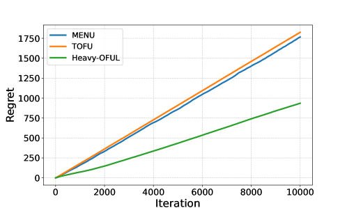
Figure 1: Comparisons of our algorithm (Heavy-OFUL) versus MENU and TOFU in heavy-tailed linear bandits problems for $1\times 10^{4}$ rounds.

We generate $5$ independent paths for each algorithm and show the average cumulative regret. The experimental setup is as follows: Let the feature dimension $d=10$. For the chosen arm $\bm{\phi}_{t}\in\mathcal{D}_{t}$, reward is $R_{t}=\langle\bm{\phi}_{t},\bm{\theta}^{*}\rangle+\varepsilon_{t}$, where $\bm{\theta}^{*}=\mathbf{1}_{d}/\sqrt{d}\in\mathbb{R}^{d}$ so that $\|\bm{\theta}^{*}\|_{2}=1$. $\varepsilon_{t}$ is first sampled from a Student’s $t$-distribution with degree of freedom $\text{df}=2$, then is multiplied by a scaling factor $\alpha$ such that the central moments of $\varepsilon_{t}$ in each rounds are different, where $\log_{10}(\alpha)\sim\mathrm{Unif}(0,2)$. Note the variance of $\varepsilon_{t}$ does not exist and we choose $\epsilon=0.99$. Normalization is made to ensure $L=B=1$. As shown in Figure 1, results demonstrate the effectiveness of the proposed algorithm, which further corroborates our theoretical findings.

Appendix B Proofs for Section 4

B.1 Properties of Huber Loss

The following properties of Huber loss are important in the proofs.

Property 1.

Denote $\Psi_{\tau}(x)$ as the derivative of Huber loss, i.e., $\Psi_{\tau}(x):=\ell^{\prime}_{\tau}(x)$, where $\Psi_{\tau}(x)$ is Huber loss defined in Definition 4.1. Then the followings are true:

1. $|\Psi_{\tau}(x)|=\min\{|x|,\tau\}$,

2. $\Psi_{\tau}(x)=\tau\Psi_{1}(\frac{x}{\tau})$,

3. $-\log(1-x+|x|^{1+\epsilon})\leq\Psi_{1}(x)\leq\log(1+x+|x|^{1+\epsilon})$ for any $\epsilon\in(0,1],$

4. $\Psi^{\prime}_{\tau}(x)=\ell_{\tau}^{\prime\prime}(x)=\operatorname{\mathds{1}}\{|x|\leq\tau\}$.

Here, (1) gives an upper bound of the derivative of Huber loss. (2) demonstrates the homogeneous property. (3) shows the similarity between the derivative of Huber loss and influence function in Catoni (2012), thereby motivating us to study the moment generating function for characterizing the noise distributions (See details in the proof of Lemma B.4 in Appendix B.6). And (4) is to characterize the second derivative of Huber loss.

B.2 Proof of Theorem 4.3

Parameters for Adaptive Huber Regression.

First, we set the parameters in Algorithm 1 as follows:

$$c_{0}=\frac{1}{\sqrt{23\log\frac{2T^{2}}{\delta}}},\quad c_{1}=\frac{(\log 3T)^{\frac{1-\epsilon}{1+\epsilon}}}{48\left(\log\frac{2T^{2}}{\delta}\right)^{\frac{2}{1+\epsilon}}},\quad\tau_{0}=\frac{\sqrt{2\kappa}b(\log 3T)^{\frac{1-\epsilon}{2(1+\epsilon)}}}{\left(\log\frac{2T^{2}}{\delta}\right)^{\frac{1}{1+\epsilon}}}.$$

Then, we give the proof of Theorem 4.3.

Proof of Theorem 4.3.

Denote $z_{t}(\bm{\theta}):=\frac{y_{t}-\langle\bm{\phi}_{t},\bm{\theta}\rangle}{\sigma_{t}}$. By the definition of $b$ and $\sigma_{t}$ in Line  ‣ 1 and 3 of Algorithm 1, respectively,

$$\mathbb{E}[{|z_{t}(\bm{\theta}^{*})|^{1+\epsilon}|\mathcal{F}_{t-1}}]=\mathbb{E}\left[\left|\frac{\varepsilon_{t}}{\sigma_{t}}\right|^{1+\epsilon}\bigg{|}\mathcal{F}_{t-1}\right]\leq b^{1+\epsilon}.$$

Notice the gradient of $L_{t}(\bm{\theta})$ is give by

$$\nabla L_{t}(\bm{\theta})=\lambda\bm{\theta}-\sum_{s=1}^{t}\frac{\bm{\phi}_{s}}{\sigma_{s}}\Psi_{\tau_{s}}(z_{s}(\bm{\theta})).$$ (B.1)

Recall $\bm{\theta}_{t}$ is the solution of Line 6 in Algorithm 1, which is a constrained convex optimization problem. Thus it holds that $\langle\nabla L_{t}(\bm{\theta}_{t}),\bm{\theta}_{t}-\bm{\theta}\rangle\leq 0,\,\,\forall\bm{\theta}\in\mathcal{B}_{d}(B)$. Since $\|\bm{\theta}^{*}\|\leq B$, we have

$$\langle\nabla L_{t}(\bm{\theta}_{t}),\bm{\theta}_{t}-\bm{\theta}^{*}\rangle\leq 0.$$ (B.2)

By the mean value theorem for vector-valued functions, we have

$$\nabla L_{t}(\bm{\theta}_{t})-\nabla L_{t}(\bm{\theta}^{*})=\int_{0}^{1}\nabla^{2}L_{t}((1-\eta)\bm{\theta}^{*}+\eta\bm{\theta}_{t})\mathrm{d}\eta\cdot(\bm{\theta}_{t}-\bm{\theta}^{*}).$$ (B.3)

In Lemma B.1, we prove that $\nabla^{2}L_{t}(\bm{\theta})$ approximates $\bm{H}_{t}$ well as long as $\bm{\theta}\in\mathcal{B}_{d}(B)$.

Lemma B.1.

Assume $\mathbb{E}[z_{t}(\bm{\theta}^{*})|\mathcal{F}_{t-1}]=0$ and $\mathbb{E}[|z_{t}(\bm{\theta}^{*})|^{1+\epsilon}|\mathcal{F}_{t-1}]\leq b^{1+\epsilon}$, set

$$\tau_{0}\geq\frac{\sqrt{2\kappa}b(\log 3T)^{\frac{1-\epsilon}{2(1+\epsilon)}}}{\left(\log\frac{2T^{2}}{\delta}\right)^{\frac{1}{1+\epsilon}}},\quad c_{0}\leq\frac{1}{\sqrt{23\log\frac{2T^{2}}{\delta}}},\quad c_{1}\leq\frac{(\log 3T)^{\frac{1-\epsilon}{1+\epsilon}}}{48\left(\log\frac{2T^{2}}{\delta}\right)^{\frac{2}{1+\epsilon}}}.$$

Then with probability at least $1-\delta$, for all $t\leq T$ and $\bm{\theta}\in\mathcal{B}_{d}(B)$, we have

$$\frac{1}{3}\bm{H}_{t}\preceq\nabla^{2}L_{t}(\bm{\theta})\preceq\bm{H}_{t}.$$

Proof.

See Appendix B.4 for a detailed proof. ∎

We set $\tau_{0},c_{0},c_{1}$ to follow Lemma B.1. Lemma B.1 implies that for all $t\leq T$ and $\eta\in[0,1]$, we have

$$\nabla^{2}L_{t}((1-\eta)\bm{\theta}^{*}+\eta\bm{\theta}_{t})\succeq\frac{1}{3}\bm{H}_{t}.$$

Thus, multiplying $\bm{\theta}_{t}-\bm{\theta}^{*}$ in both sides of (B.3) yields

$$\langle\bm{\theta}_{t}-\bm{\theta}^{*},\nabla L_{t}(\bm{\theta}_{t})-\nabla L_{t}(\bm{\theta}^{*})\rangle$$ (B.4)

$$={} \langle\bm{\theta}_{t}-\bm{\theta}^{*},\int_{0}^{1}\nabla^{2}L_{t}((1-\eta)\bm{\theta}^{*}+\eta\bm{\theta}_{t})\mathrm{d}\eta\cdot(\bm{\theta}_{t}-\bm{\theta}^{*})\rangle$$

$$\geq{} \langle\bm{\theta}_{t}-\bm{\theta}^{*},\frac{1}{3}\bm{H}_{t}\cdot(\bm{\theta}_{t}-\bm{\theta}^{*})\rangle$$

$$={} \frac{1}{3}\|\bm{\theta}_{t}-\bm{\theta}^{*}\|_{\bm{H}_{t}}^{2}.$$

On the other hand, by (B.2), we have

$$\langle\bm{\theta}_{t}-\bm{\theta}^{*},\nabla L_{t}(\bm{\theta}_{t})-\nabla L_{t}(\bm{\theta}^{*})\rangle\leq\langle\bm{\theta}_{t}-\bm{\theta}^{*},-\nabla L_{t}(\bm{\theta}^{*})\rangle\leq\|\bm{\theta}_{t}-\bm{\theta}^{*}\|_{\bm{H}_{t}}\cdot\|\nabla L_{t}(\bm{\theta}^{*})\|_{\bm{H}_{t}^{-1}}.$$

That implies

$$\|\bm{\theta}_{t}-\bm{\theta}^{*}\|_{\bm{H}_{t}}\leq 3\|\nabla L_{t}(\bm{\theta}^{*})\|_{\bm{H}_{t}^{-1}}.$$ (B.5)

Next we use Lemma B.2 to give a high probability upper bound of $\|\nabla L_{t}(\bm{\theta}^{*})\|_{\bm{H}_{t}^{-1}}$.

Lemma B.2.

Assume $\mathbb{E}[z_{t}(\bm{\theta}^{*})|\mathcal{F}_{t-1}]=0$, $\mathbb{E}[|z_{t}(\bm{\theta}^{*})|^{1+\epsilon}|\mathcal{F}_{t-1}]\leq b^{1+\epsilon}$ and

$$\tau_{0}\geq\frac{\sqrt{2\kappa}b(\log 3T)^{\frac{1-\epsilon}{2(1+\epsilon)}}}{\left(\log\frac{2T^{2}}{\delta}\right)^{\frac{1}{1+\epsilon}}},$$

then with probability at least $1-2\delta,\forall t\geq 1$, we have

$$\|\nabla L_{t}(\bm{\theta}^{*})\|_{\bm{H}_{t}^{-1}}\leq\sqrt{\lambda}B+\alpha_{t},$$

where

$$\alpha_{t}=4t^{\frac{1-\epsilon}{2(1+\epsilon)}}\left[\frac{(\sqrt{2\kappa}b)^{1+\epsilon}(\log 3t)^{\frac{1-\epsilon}{2}}}{\tau_{0}^{\epsilon}}+\tau_{0}\log\frac{2t^{2}}{\delta}\right].$$

Proof.

See Appendix B.5 for a detailed proof. ∎

Notice the conditions of Lemma B.2 are satisfied. On the event where Lemma B.1 and B.2 hold, whose probability is at least $1-3\delta$, combining (B.5) and Lemma B.2 gives

$$\|\bm{\theta}_{t}-\bm{\theta}^{*}\|_{\bm{H}_{t}}\leq 3\sqrt{\lambda}B+12t^{\frac{1-\epsilon}{2(1+\epsilon)}}\left[\frac{(\sqrt{2\kappa}b)^{1+\epsilon}(\log 3t)^{\frac{1-\epsilon}{2}}}{\tau_{0}^{\epsilon}}+\tau_{0}\log\frac{2t^{2}}{\delta}\right].$$

Choosing $\tau_{0}=\frac{\sqrt{2\kappa}b(\log 3T)^{\frac{1-\epsilon}{2(1+\epsilon)}}}{\left(\log\frac{2T^{2}}{\delta}\right)^{\frac{1}{1+\epsilon}}}$ gives the final result. ∎

B.3 Perturbation Analysis of Adaptive Huber Regression

Lemma B.3.

Consider the setting in Definition 4.2. Let $L_{t}(\cdot),\bm{\theta}_{t}$ be defined in Theorem 4.3. Define $\widehat{L}_{t}(\bm{\theta}):=\frac{\lambda}{2}\|\bm{\theta}\|^{2}+\sum_{s=1}^{t}\ell_{\tau_{s}}\left(\frac{\widehat{y}_{s}-\langle\bm{\phi}_{s},\bm{\theta}\rangle}{\sigma_{s}}\right)$, where the parameters $\tau_{s},\sigma_{s}$ are chosen according to Theorem 4.3. $\widehat{L}_{t}(\cdot)$ is the same as $L_{t}(\cdot)$ except for substituting $y_{s}$ with $\widehat{y}_{s}\in\mathcal{F}_{s}$. And let $\widehat{\bm{\theta}}_{t}:=\mathop{\mathrm{argmin}}_{\bm{\theta}\in\mathcal{B}_{d}(B)}\widehat{L}_{t}(\bm{\theta})$. Suppose $\left|\widehat{y}_{s}-y_{s}\right|\leq\widehat{\beta}_{s}\left\|\bm{\phi}_{s}\right\|_{\bm{H}_{s}^{-1}}$ for $s\leq t$. Then, under the event where Theorem 4.3 holds, we have

$$\|\widehat{\bm{\theta}}_{t}-\bm{\theta}_{t}\|_{\bm{H}_{t}}\leq 6\kappa\max_{s\leq t}\widehat{\beta}_{s}.$$

Proof.

Notice $\bm{\theta}_{t}$ and $\widehat{\bm{\theta}}_{t}$ are solutions of convex optimization problems, we have

$$\langle\nabla L_{t}(\bm{\theta}_{t}),\bm{\theta}_{t}-\widehat{\bm{\theta}}_{t}\rangle\leq 0,\quad\langle\nabla\widehat{L}_{t}(\widehat{\bm{\theta}}_{t}),\widehat{\bm{\theta}}_{t}-\bm{\theta}_{t}\rangle\leq 0.$$ (B.6)

With a similar argument as for (LABEL:eq:hessian-approx) in the proof of Theorem 4.3 in Appendix B.2, on the event where Theorem 4.3 holds, we have

$$\langle\bm{\theta}_{t}-\widehat{\bm{\theta}}_{t},\nabla L_{t}(\bm{\theta})-\nabla L_{t}(\widehat{\bm{\theta}}_{t})\rangle\geq\frac{1}{3}\|\bm{\theta}_{t}-\widehat{\bm{\theta}}_{t}\|_{\bm{H}_{t}}^{2}.$$

Combined with (B.6), it holds that

$$\|\bm{\theta}_{t}-\widehat{\bm{\theta}}_{t}\|_{\bm{H}_{t}}^{2}\leq 3\langle\bm{\theta}_{t}-\widehat{\bm{\theta}}_{t},\nabla\widehat{L}_{t}(\widehat{\bm{\theta}}_{t})-\nabla L_{t}(\widehat{\bm{\theta}}_{t})\rangle\leq 3\|\bm{\theta}_{t}-\widehat{\bm{\theta}}_{t}\|_{\bm{H}_{t}}\|\nabla\widehat{L}_{t}(\widehat{\bm{\theta}}_{t})-\nabla L_{t}(\widehat{\bm{\theta}}_{t})\|_{\bm{H}_{t}^{-1}}.$$

Thus

$$\|\bm{\theta}_{t}-\widehat{\bm{\theta}}_{t}\|_{\bm{H}_{t}} \leq 3\|\nabla\widehat{L}_{t}(\widehat{\bm{\theta}}_{t})-\nabla L_{t}(\widehat{\bm{\theta}}_{t})\|_{\bm{H}_{t}^{-1}}$$

$$=3\left\|\sum_{s=1}^{t}\frac{\bm{\phi}_{s}}{\sigma_{s}}\left[\Psi_{\tau_{s}}\left(\frac{\widehat{y}_{s}-\langle\phi_{s},\widehat{\bm{\theta}}_{t}\rangle}{\sigma_{s}}\right)-\Psi_{\tau_{s}}\left(\frac{y_{s}-\langle\phi_{s},\widehat{\bm{\theta}}_{t}\rangle}{\sigma_{s}}\right)\right]\right\|_{\bm{H}_{t}^{-1}}$$

$$\overset{(a)}{\leq}3\left\|\sum_{s=1}^{t}\frac{\bm{\phi}_{s}}{\sigma_{s}}\left|\frac{\widehat{y}_{s}-y_{s}}{\sigma_{s}}\right|\right\|_{\bm{H}_{t}^{-1}}$$

$$\overset{(b)}{\leq}3\cdot(\max_{s\leq t}\widehat{\beta}_{s})\cdot\left\|\sum_{s=1}^{t}\frac{\bm{\phi}_{s}}{\sigma_{s}}\cdot\left\|\frac{\bm{\phi}_{s}}{\sigma_{s}}\right\|_{\bm{H}_{s}^{-1}}\right\|_{\bm{H}_{t}^{-1}}$$

$$\leq 3\cdot(\max_{s\leq t}\widehat{\beta}_{s})\cdot\sum_{s=1}^{t}\left\|\frac{\bm{\phi}_{s}}{\sigma_{s}}\right\|_{\bm{H}_{t}^{-1}}\cdot\left\|\frac{\bm{\phi}_{s}}{\sigma_{s}}\right\|_{\bm{H}_{s}^{-1}}$$

where $(a)$ is due to (1) of Property 1 and $(b)$ uses the condition that $|\widehat{y}_{s}-y_{s}|\leq\widehat{\beta}_{s}\left\|\bm{\phi}_{s}\right\|_{\bm{H}_{s}^{-1}}$. Notice $\bm{H}_{t}^{-1}\preceq\bm{H}_{s}^{-1}$ for $s\leq t$, we have $\left\|\frac{\bm{\phi}_{s}}{\sigma_{s}}\right\|_{\bm{H}_{t}^{-1}}\leq\left\|\frac{\bm{\phi}_{s}}{\sigma_{s}}\right\|_{\bm{H}_{s}^{-1}}$, which further implies

$$\left\|\frac{\bm{\phi}_{s}}{\sigma_{s}}\right\|_{\bm{H}_{s}^{-1}}^{2}=\frac{\bm{\phi}_{s}^{\top}}{\sigma_{s}}\left(\bm{H}_{s-1}^{-1}-\frac{\bm{H}_{s-1}^{-1}\frac{\bm{\phi}_{s}}{\sigma_{s}}\frac{\bm{\phi}_{s}^{\top}}{\sigma_{s}}\bm{H}_{s-1}^{-1}}{1+\frac{\bm{\phi}_{s}^{\top}}{\sigma_{s}}\bm{H}_{s-1}^{-1}\frac{\bm{\phi}_{s}^{\top}}{\sigma_{s}}}\right)\frac{\bm{\phi}_{s}}{\sigma_{s}}=w_{s}^{2}-\frac{w_{s}^{4}}{1+w_{s}^{2}}=\frac{w_{s}^{2}}{1+w_{s}^{2}}$$ (B.7)

due to Sherman-Morrison formula with $w_{t}=\|\bm{\phi}_{t}/\sigma_{t}\|_{\bm{H}_{t-1}^{-1}}$. Then It follows that

$$\sum_{s=1}^{t}\left\|\frac{\bm{\phi}_{s}}{\sigma_{s}}\right\|_{\bm{H}_{t}^{-1}}\cdot\left\|\frac{\bm{\phi}_{s}}{\sigma_{s}}\right\|_{\bm{H}_{s}^{-1}}\leq\sum_{s=1}^{t}\frac{w_{s}^{2}}{1+w_{s}^{2}}\leq\sum_{s=1}^{t}\min\left\{1,w_{s}^{2}\right\}\leq 2\kappa,$$

where the last inequality holds due to Lemma H.6. Finally, we have

$$\|\bm{\theta}_{t}-\widehat{\bm{\theta}}_{t}\|_{\bm{H}_{t}}\leq 6\kappa\max_{s\leq t}\widehat{\beta}_{s}.$$

∎

B.4 Proof of Lemma B.1

In the following proof, we denote $z_{t}^{*}:=z_{t}(\bm{\theta}^{*})=\frac{y_{t}-\langle\bm{\phi}_{t},\bm{\theta}^{*}\rangle}{\sigma_{t}}=\frac{\varepsilon_{t}}{\sigma_{t}}$ for short.

Proof of Lemma B.1.

Using (4) of Property 1, the Hessian matrix of $L_{t}(\bm{\theta})$ is given by

$$\nabla^{2}L_{t}(\bm{\theta})=\lambda\bm{I}+\sum_{s=1}^{t}\frac{1}{\sigma_{s}^{2}}\bm{\phi}_{s}\bm{\phi}_{s}^{\top}\operatorname{\mathds{1}}\{|z_{s}(\bm{\theta})|\leq\tau_{s}\}=\bm{H}_{t}-\sum_{s=1}^{t}\frac{1}{\sigma_{s}^{2}}\bm{\phi}_{s}\bm{\phi}_{s}^{\top}\operatorname{\mathds{1}}\{|z_{s}(\bm{\theta})|>\tau_{s}\}.$$ (B.8)

Thus

$$\nabla^{2}L_{t}(\bm{\theta})\preceq\bm{H}_{t}$$

holds trivially. And we only need to prove

$$\nabla^{2}L_{t}(\bm{\theta})\succeq\frac{1}{3}\bm{H}_{t}.$$

We can decompose $z_{s}(\bm{\theta})$ as

$$z_{s}(\bm{\theta})=\frac{y_{s}-\langle\bm{\phi}_{s},\bm{\theta}\rangle}{\sigma_{s}}=\frac{\varepsilon_{s}+\langle\bm{\phi}_{s},\bm{\theta}^{*}-\bm{\theta}\rangle}{\sigma_{s}}=z_{s}^{*}+\frac{\langle\bm{\phi}_{s},\bm{\theta}^{*}-\bm{\theta}\rangle}{\sigma_{s}}.$$

Then notice

$$\operatorname{\mathds{1}}\{|z_{s}(\bm{\theta})|>\tau_{s}\}\leq\operatorname{\mathds{1}}\left\{|z_{s}^{*}|>\frac{\tau_{s}}{2}\right\}+\operatorname{\mathds{1}}\left\{\left|\frac{\langle\bm{\phi}_{s},\bm{\theta}-\bm{\theta}^{*}\rangle}{\sigma_{s}}\right|>\frac{\tau_{s}}{2}\right\}.$$

For all $\bm{u}\in\mathcal{B}_{d}(1)$, we have

$$\bm{u}^{\top}\nabla^{2}L_{t}(\bm{\theta})\bm{u}=\bm{u}^{\top}\bm{H}_{t}\bm{u}-\sum_{s=1}^{t}\frac{\langle\bm{\phi}_{s},\bm{u}\rangle^{2}}{\sigma_{s}^{2}}\operatorname{\mathds{1}}\{|z_{s}(\bm{\theta})|>\tau_{s}\}$$

$$\geq{} \bm{u}^{\top}\bm{H}_{t}\bm{u}-\underbrace{\sum_{s=1}^{t}\frac{\langle\bm{\phi}_{s},\bm{u}\rangle^{2}}{\sigma_{s}^{2}}\operatorname{\mathds{1}}\left\{|z_{s}^{*}|>\frac{\tau_{s}}{2}\right\}}_{\text{(i)}}-\underbrace{\sum_{s=1}^{t}\frac{\langle\bm{\phi}_{s},\bm{u}\rangle^{2}}{\sigma_{s}^{2}}\operatorname{\mathds{1}}\left\{\left|\frac{\langle\bm{\phi}_{s},\bm{\theta}-\bm{\theta}^{*}\rangle}{\sigma_{s}}\right|>\frac{\tau_{s}}{2}\right\}}_{\text{(ii)}}.$$

Next we establish upper bounds for term (i) and (ii) respectively.

Term (i).

Notice

$$\sum_{s=1}^{t}\frac{\langle\bm{\phi}_{s},\bm{u}\rangle^{2}}{\sigma_{s}^{2}}\operatorname{\mathds{1}}\left\{|z_{s}^{*}|>\frac{\tau_{s}}{2}\right\} \overset{(a)}{\leq}\sum_{s=1}^{t}\left\|\frac{\bm{\phi}_{s}}{\sigma_{s}}\right\|_{\bm{H}_{t}^{-1}}^{2}\|\bm{u}\|_{\bm{H}_{t}}^{2}\operatorname{\mathds{1}}\left\{|z_{s}^{*}|>\frac{\tau_{s}}{2}\right\}$$ (B.9)

$$\overset{(b)}{=}\|\bm{u}\|_{\bm{H}_{t}}^{2}\sum_{s=1}^{t}\frac{w_{s}^{2}}{1+w_{s}^{2}}\operatorname{\mathds{1}}\left\{|z_{s}^{*}|>\frac{\tau_{s}}{2}\right\}$$

$$\overset{(c)}{\leq}c_{0}^{2}\|\bm{u}\|_{\bm{H}_{t}}^{2}\sum_{s=1}^{t}\operatorname{\mathds{1}}\left\{|z_{s}^{*}|>\frac{\tau_{s}}{2}\right\},$$

where $(a)$ holds due to the Cauchy-Schwartz inequality, $(b)$ holds with the same argument as (B.7), while $(c)$ holds due to $\frac{w_{s}^{2}}{1+w_{s}^{2}}\leq w_{s}^{2}$ and our choice of $\sigma_{s}$ in Line 3 of Algorithm 1 such that $\sigma_{s}\geq\frac{\left\|\bm{\phi}_{s}\right\|_{\bm{H}_{s-1}^{-1}}}{c_{0}}$.

Next we give an upper bound of $\sum_{s=1}^{t}\operatorname{\mathds{1}}\{|z_{s}^{*}|>\frac{\tau_{s}}{2}\}$. Define $X_{s}:=\operatorname{\mathds{1}}\{|z_{s}^{*}|>\frac{\tau_{s}}{2}\}$ and $Y_{s}:=X_{s}-\mathbb{E}[X_{s}|\mathcal{F}_{s-1}]$, which are $\mathcal{F}_{s}$-measurable. Lemma H.1 implies that with probability at least $1-2t^{2}/\delta,\text{for any fixed }t\geq 1$, we have

$$\sum_{s=1}^{t}Y_{s}\leq\sqrt{2V\log\frac{2t^{2}}{\delta}}+\frac{2M}{3}\log\frac{2t^{2}}{\delta},$$ (B.10)

where $\sum_{s=1}^{t}\mathbb{E}[Y_{s}^{2}|\mathcal{F}_{s-1}]\leq V\text{ and }|Y_{t}|\leq M$. It follows that $|Y_{s}|\leq 1$ and

$$\sum_{s=1}^{t}\mathbb{E}[X_{s}|\mathcal{F}_{s-1}] =\sum_{s=1}^{t}\mathbb{P}\left(|z_{s}^{*}|>\frac{\tau_{s}}{2}\right)$$

$$\overset{(a)}{\leq}2^{1+\epsilon}\sum_{s=1}^{t}\frac{b^{1+\epsilon}}{\tau_{s}^{1+\epsilon}}$$

$$\overset{(b)}{=}\left(\frac{2b}{\tau_{0}}\right)^{1+\epsilon}\sum_{s=1}^{t}\left(\frac{w_{s}}{\sqrt{1+w_{s}^{2}}}\right)^{1+\epsilon}s^{-\frac{1-\epsilon}{2}},$$

where $(a)$ holds due to Markov’s inequality and $(b)$ holds due to the definition of $\tau_{s}$ in Line 4 of Algorithm 1. Notice

$$\sum_{s=1}^{t}\left(\frac{w_{s}}{\sqrt{1+w_{s}^{2}}}\right)^{1+\epsilon}s^{-\frac{1-\epsilon}{2}}\leq\left(\sum_{s=1}^{t}\frac{w_{s}^{2}}{1+w_{s}^{2}}\right)^{\frac{1+\epsilon}{2}}\left(\sum_{s=1}^{t}s^{-1}\right)^{\frac{1-\epsilon}{2}}\leq(2\kappa)^{\frac{1+\epsilon}{2}}(\log 3t)^{\frac{1-\epsilon}{2}},$$ (B.11)

where the first inequality holds due to Hölder’s inequality and the second holds due to $\frac{w_{s}^{2}}{1+w_{s}^{2}}\leq\min\{1,w_{s}^{2}\}$, Lemma H.6 and $\sum_{s=1}^{t}s^{-1}\leq 1+\log t\leq\log 3t$. Thus

$$\sum_{s=1}^{t}\mathbb{E}[X_{s}|\mathcal{F}_{s-1}]\leq\left(\frac{2b}{\tau_{0}}\right)^{1+\epsilon}(2\kappa)^{\frac{1+\epsilon}{2}}(\log 3t)^{\frac{1-\epsilon}{2}}=\left(\frac{2\sqrt{2\kappa}b(\log 3t)^{\frac{1-\epsilon}{2(1+\epsilon)}}}{\tau_{0}}\right)^{1+\epsilon}.$$

Then it follows that

$$\sum_{s=1}^{t}\mathbb{E}[Y_{s}^{2}|\mathcal{F}_{s-1}]\leq\sum_{s=1}^{t}\mathbb{E}[X_{s}^{2}|\mathcal{F}_{s-1}]=\sum_{s=1}^{t}\mathbb{E}[X_{s}|\mathcal{F}_{s-1}].$$

Setting $V=\left(\frac{2\sqrt{2\kappa}b(\log 3t)^{\frac{1-\epsilon}{2(1+\epsilon)}}}{\tau_{0}}\right)^{1+\epsilon}$ and $M=1$ in (B.10), using a union bound over $t\geq 1$ and the fact that $\sum_{t=1}^{\infty}\frac{1}{2t^{2}}\leq 1$, with probability at least $1-\delta,\forall t\geq 1$, we have

$$\sum_{s=1}^{t}\operatorname{\mathds{1}}\left\{|z_{s}^{*}|>\frac{\tau_{s}}{2}\right\}=\sum_{s=1}^{t}X_{s}$$ (B.12)

$$\leq{} \sum_{s=1}^{t}\mathbb{E}[X_{s}|\mathcal{F}_{s-1}]+\sqrt{2V\log\frac{2t^{2}}{\delta}}+\frac{2M}{3}\log\frac{2t^{2}}{\delta}$$

$$={} \left(\frac{2\sqrt{2\kappa}b(\log 3t)^{\frac{1-\epsilon}{2(1+\epsilon)}}}{\tau_{0}}\right)^{1+\epsilon}+\sqrt{2\left(\frac{2\sqrt{2\kappa}b(\log 3t)^{\frac{1-\epsilon}{2(1+\epsilon)}}}{\tau_{0}}\right)^{1+\epsilon}\log\frac{2t^{2}}{\delta}}+\frac{2}{3}\log\frac{2t^{2}}{\delta}.$$

Choosing $\tau_{0}\geq\frac{\sqrt{2\kappa}b(\log 3T)^{\frac{1-\epsilon}{2(1+\epsilon)}}}{\left(\log\frac{2T^{2}}{\delta}\right)^{\frac{1}{1+\epsilon}}}$ yields $\left(\frac{2\sqrt{2\kappa}b(\log 3t)^{\frac{1-\epsilon}{2(1+\epsilon)}}}{\tau_{0}}\right)^{1+\epsilon}\leq 2^{1+\epsilon}\log\frac{2T^{2}}{\delta}$.

Then it follows from (B.9) and (B.12) that

$$\sum_{s=1}^{t}\frac{\langle\bm{\phi}_{s},\bm{u}\rangle^{2}}{\sigma_{s}^{2}}\operatorname{\mathds{1}}\left\{|z_{s}^{*}|>\frac{\tau_{s}}{2}\right\} \leq c_{0}^{2}\|\bm{u}\|_{\bm{H}_{t}}^{2}\sum_{s=1}^{t}\operatorname{\mathds{1}}\left\{|z_{s}^{*}|>\frac{\tau_{s}}{2}\right\}$$

$$\leq c_{0}^{2}\|\bm{u}\|_{\bm{H}_{t}}^{2}\left(2^{1+\epsilon}+\sqrt{2\cdot 2^{1+\epsilon}}+\frac{2}{3}\right)\log\frac{2T^{2}}{\delta}$$

$$\leq\frac{23}{3}c_{0}^{2}\log\frac{2T^{2}}{\delta}\|\bm{u}\|_{\bm{H}_{t}}^{2}$$

$$\leq\frac{1}{3}\|\bm{u}\|_{\bm{H}_{t}}^{2},$$

where the third inequality holds due to $\epsilon\leq 1$ and the last holds due to the definition of $c_{0}$.

Term (ii).

$$\sum_{s=1}^{t}\frac{\langle\bm{\phi}_{s},\bm{u}\rangle^{2}}{\sigma_{s}^{2}}\operatorname{\mathds{1}}\left\{\left|\frac{\langle\bm{\phi}_{s},\bm{\theta}-\bm{\theta}^{*}\rangle}{\sigma_{s}}\right|>\frac{\tau_{s}}{2}\right\} \leq\sum_{s=1}^{t}\frac{\langle\bm{\phi}_{s},\bm{u}\rangle^{2}}{\sigma_{s}^{2}}\frac{\langle\bm{\phi}_{s},\bm{\theta}-\bm{\theta}^{*}\rangle^{2}}{\sigma_{s}^{2}}\frac{4}{\tau_{s}^{2}}$$ (B.13)

$$\overset{(a)}{\leq}16\sum_{s=1}^{t}\frac{\langle\bm{\phi}_{s},\bm{u}\rangle^{2}}{\sigma_{s}^{2}}\frac{L^{2}B^{2}}{\sigma_{s}^{2}\tau_{0}^{2}}\frac{w_{s}^{2}}{1+w_{s}^{2}}s^{-\frac{1-\epsilon}{1+\epsilon}}$$

$$\overset{(b)}{\leq}16\sum_{s=1}^{t}\frac{\langle\bm{\phi}_{s},\bm{u}\rangle^{2}}{\sigma_{s}^{2}}\frac{L^{2}B^{2}w_{s}^{2}}{\sigma_{s}^{2}\cdot 2\kappa b^{2}}\frac{2\kappa b^{2}}{\tau_{0}^{2}}$$

$$\overset{(c)}{\leq}16\sum_{s=1}^{t}\frac{\langle\bm{\phi}_{s},\bm{u}\rangle^{2}}{\sigma_{s}^{2}}c_{1}\frac{2\kappa b^{2}}{\tau_{0}^{2}}$$

$$\overset{(d)}{\leq}\frac{1}{3}\sum_{s=1}^{t}\frac{\langle\bm{\phi}_{s},\bm{u}\rangle^{2}}{\sigma_{s}^{2}},$$

where $(a)$ holds due to Cauchy-Schwartz inequality with $\|\bm{\phi}_{s}\|\leq L$, $\|\bm{\theta}-\bm{\theta}^{*}\|\leq 2B$ and the definition of $\tau_{s}$ in Line 4 of Algorithm 1. $(b)$ holds due to $\frac{1}{1+w_{s}^{2}}s^{-\frac{1-\epsilon}{1+\epsilon}}\leq 1$. $(c)$ uses the definition of $\sigma_{s}$ in Line 3 in Algorithm 1, that is $\frac{L^{2}B^{2}w_{s}^{2}}{\sigma_{s}^{2}\cdot 2\kappa b^{2}}\leq c_{1}$ implied by $\sigma_{s}\geq\frac{\sqrt{LB}\|\bm{\phi}_{s}\|_{\bm{H}_{s-1}^{-1}}^{\frac{1}{2}}}{c_{1}^{\frac{1}{4}}(2\kappa b^{2})^{\frac{1}{4}}}$. $(d)$ holds due to our choice of $\tau_{0}$ and $c_{1}$.

Putting pieces together.

Combining (B.12) and (B.13), with probability at least $1-\delta$, for all $t\leq T,\bm{\theta}\in\mathcal{B}_{d}(B)$ and $\bm{u}\in\mathcal{B}_{d}(1)$, we have

$$\bm{u}^{\top}\nabla^{2}L_{t}(\bm{\theta})\bm{u}$$

$$\geq{} \bm{u}^{\top}\bm{H}_{t}\bm{u}-\sum_{s=1}^{t}\frac{\langle\bm{\phi}_{s},\bm{u}\rangle^{2}}{\sigma_{s}^{2}}\operatorname{\mathds{1}}\left\{|z_{s}^{*}|>\frac{\tau_{s}}{2}\right\}-\sum_{s=1}^{t}\frac{\langle\bm{\phi}_{s},\bm{u}\rangle^{2}}{\sigma_{s}^{2}}\operatorname{\mathds{1}}\left\{\left|\frac{\langle\bm{\phi}_{s},\bm{\theta}-\bm{\theta}^{*}\rangle}{\sigma_{s}}\right|>\frac{\tau_{s}}{2}\right\}.$$

$$\geq{} \bm{u}^{\top}\bm{H}_{t}\bm{u}-\frac{1}{3}\bm{u}^{\top}\bm{H}_{t}\bm{u}-\frac{1}{3}\sum_{s=1}^{t}\frac{\langle\bm{\phi}_{s},\bm{u}\rangle^{2}}{\sigma_{s}^{2}}$$

$$\geq{} \frac{2}{3}\bm{u}^{\top}\bm{H}_{t}\bm{u}-\frac{1}{3}\left(\lambda\|\bm{u}\|^{2}+\sum_{s=1}^{t}\frac{\langle\bm{\phi}_{s},\bm{u}\rangle^{2}}{\sigma_{s}^{2}}\right)$$

$$={} \frac{1}{3}\bm{u}^{\top}\bm{H}_{t}\bm{u},$$

which implies $\nabla^{2}L_{t}(\bm{\theta})\succeq\frac{1}{3}\bm{H}_{t}$. ∎

B.5 Proof of Lemma B.2

Proof of Lemma B.2.

The expression of $\nabla L_{t}(\bm{\theta})$ in (B.1) gives

$$\|\nabla L_{t}(\bm{\theta}^{*})\|_{\bm{H}_{t}^{-1}} \leq\lambda\|\bm{\theta}\|_{\bm{H}_{t}^{-1}}+\Bigg{\|}\underbrace{\sum_{s=1}^{t}\Psi_{\tau_{s}}(z_{s}^{*})\frac{\bm{\phi}_{s}}{\sigma_{s}}}_{\bm{d}_{t}}\Bigg{\|}_{\bm{H}_{t}^{-1}}.$$

We next construct upper bounds of $\lambda\|\bm{\theta}\|_{\bm{H}_{t}^{-1}}$ and $\|\bm{d}_{t}\|_{\bm{H}_{t}^{-1}}$, respectively.

Bound $\lambda\|\bm{\theta}\|_{\bm{H}_{t}^{-1}}$.

Since $\bm{H}_{t}\succeq\lambda\bm{I}$, we have $\bm{H}_{t}^{-1}\preceq\frac{1}{\lambda}\bm{I}$. Thus, $\lambda\|\bm{\theta}\|_{\bm{H}_{t}^{-1}}\leq\lambda\frac{1}{\sqrt{\lambda}}\|\bm{\theta}\|\leq\sqrt{\lambda}B$.

Bound $\|\bm{d}_{t}\|_{\bm{H}_{t}^{-1}}$.

We aim to decompose $\|\bm{d}_{t}\|_{\bm{H}_{t}^{-1}}^{2}$ into two terms and bound them separately. The fact that $\bm{H}_{t}=\bm{H}_{t-1}+\frac{\bm{\phi}_{t}\bm{\phi}_{t}^{\top}}{\sigma_{t}^{2}}$ together with the Sherman-Morrison formula implies that

$$\bm{H}_{t}^{-1}=\bm{H}_{t-1}^{-1}-\frac{\bm{H}_{t-1}^{-1}\bm{\phi}_{t}\bm{\phi}_{t}^{\top}\bm{H}_{t-1}^{-1}}{\sigma_{t}^{2}(1+w_{t}^{2})},\quad\text{where }w_{t}^{2}:=\frac{\bm{\phi}_{t}^{\top}\bm{H}_{t-1}^{-1}\bm{\phi}_{t}}{\sigma_{t}^{2}}=\left\|\frac{\bm{\phi}_{t}}{\sigma_{t}}\right\|_{\bm{H}_{t-1}}^{2}.$$ (B.14)

Clearly, $w_{t}$ is $\mathcal{F}_{t-1}$-measurable and thus is predictable. By definition of $\bm{d}_{t}$ and (B.14),

$$\|\bm{d}_{t}\|_{\bm{H}_{t}^{-1}}^{2}$$ (B.15)

$$={} \left(\bm{d}_{t-1}+\Psi_{\tau_{t}}(z_{t}^{*})\frac{\bm{\phi}_{t}}{\sigma_{t}}\right)^{\top}\bm{H}_{t}^{-1}\left(\bm{d}_{t-1}+\Psi_{\tau_{t}}(z_{t}^{*})\frac{\bm{\phi}_{t}}{\sigma_{t}}\right)$$

$$={} \|\bm{d}_{t-1}\|_{\bm{H}_{t-1}^{-1}}^{2}-\frac{1}{1+w_{t}^{2}}\left(\frac{\bm{d}_{t-1}^{\top}\bm{H}_{t-1}^{-1}\bm{\phi}_{t}}{\sigma_{t}}\right)^{2}+2\Psi_{\tau_{t}}(z_{t}^{*})\frac{\bm{d}_{t-1}^{\top}\bm{H}_{t}^{-1}\bm{\phi}_{t}}{\sigma_{t}}+\Psi_{\tau_{t}}^{2}(z_{t}^{*})\frac{\bm{\phi}_{t}^{\top}\bm{H}_{t}^{-1}\bm{\phi}_{t}}{\sigma_{t}^{2}}$$

$$\leq{} \|\bm{d}_{t-1}\|_{\bm{H}_{t-1}^{-1}}^{2}+\underbrace{2\Psi_{\tau_{t}}(z_{t}^{*})\frac{\bm{d}_{t-1}^{\top}\bm{H}_{t}^{-1}\bm{\phi}_{t}}{\sigma_{t}}}_{I_{1}}+\underbrace{\Psi_{\tau_{t}}^{2}(z_{t}^{*})\frac{\bm{\phi}_{t}^{\top}\bm{H}_{t}^{-1}\bm{\phi}_{t}}{\sigma_{t}^{2}}}_{I_{2}}.$$ (B.16)

For $I_{1}$, by (B.14), we have

$$I_{1} =2\Psi_{\tau_{t}}(z_{t}^{*})\frac{1}{\sigma_{t}}\bm{d}_{t-1}^{\top}\left(\bm{H}_{t-1}^{-1}-\frac{\bm{H}_{t-1}^{-1}\bm{\phi}_{t}\bm{\phi}_{t}^{\top}\bm{H}_{t-1}^{-1}}{\sigma_{t}^{2}(1+w_{t}^{2})}\right)\bm{\phi}_{t}$$

$$=2\Psi_{\tau_{t}}(z_{t}^{*})\frac{1}{1+w_{t}^{2}}\frac{\bm{d}_{t-1}^{\top}\bm{H}_{t-1}^{-1}\bm{\phi}_{t}}{\sigma_{t}}.$$

For $I_{2}$, we have

$$I_{2} =\Psi_{\tau_{t}}^{2}(z_{t}^{*})\frac{\bm{\phi}_{t}^{\top}\bm{H}_{t}^{-1}\bm{\phi}_{t}}{\sigma_{t}^{2}}$$

$$=\Psi_{\tau_{t}}^{2}(z_{t}^{*})\frac{1}{\sigma_{t}^{2}}\bm{\phi}_{t}^{\top}\left(\bm{H}_{t-1}^{-1}-\frac{\bm{H}_{t-1}^{-1}\bm{\phi}_{t}\bm{\phi}_{t}^{\top}\bm{H}_{t-1}^{-1}}{\sigma_{t}^{2}(1+w_{t}^{2})}\right)\bm{\phi}_{t}$$

$$=\Psi_{\tau_{t}}^{2}(z_{t}^{*})\left(w_{t}^{2}-\frac{w_{t}^{4}}{1+w_{t}^{2}}\right)$$

$$=\Psi_{\tau_{t}}^{2}(z_{t}^{*})\frac{w_{t}^{2}}{1+w_{t}^{2}}.$$

Using the equations for $I_{1},I_{2}$ and iterating (B.15), we have

$$\|\bm{d}_{t}\|_{\bm{H}_{t}^{-1}}^{2}\leq\underbrace{\sum_{s=1}^{t}\Psi_{\tau_{s}}(z_{s}^{*})\frac{2}{1+w_{s}^{2}}\frac{\bm{d}_{s-1}^{\top}\bm{H}_{s-1}^{-1}\bm{\phi}_{s}}{\sigma_{s}}}_{\text{(i)}}+\underbrace{\sum_{s=1}^{t}\Psi_{\tau_{s}}^{2}(z_{s}^{*})\frac{w_{s}^{2}}{1+w_{s}^{2}}}_{\text{(ii)}}.$$

Next we use Lemma B.4 and Lemma B.5 to bound (i) and (ii), respectively. We remark that (i) is the leading term. In the proof of Lemma B.4, inspired by (Catoni, 2012; Sun et al., 2020), we make use of (3) of Property 1 to carefully quantify the moment generating function, and thus achieves a tight bound.

Lemma B.4.

Assume $\mathbb{E}[z_{t}(\bm{\theta}^{*})|\mathcal{F}_{t-1}]=0$ and $\mathbb{E}[|z_{t}(\bm{\theta}^{*})|^{1+\epsilon}|\mathcal{F}_{t-1}]\leq b^{1+\epsilon}$, let $A_{t}$ define the event where $\|\bm{d}_{s}\|_{\bm{H}_{s}^{-1}}\leq\alpha_{s}$ for $s\leq t$. Then with probability at least $1-\delta,\forall t\geq 1$, we have

$$\sum_{s=1}^{t}\Psi_{\tau_{s}}(z_{s}^{*})\frac{2\bm{d}_{s-1}^{\top}\bm{H}_{s-1}^{-1}\bm{\phi}_{s}\operatorname{\mathds{1}}_{A_{s-1}}}{(1+w_{s}^{2})\sigma_{s}}\leq(\max_{s\leq t}\alpha_{s})2t^{\frac{1-\epsilon}{2(1+\epsilon)}}\left[\frac{(\sqrt{2\kappa}b)^{1+\epsilon}(\log 3t)^{\frac{1-\epsilon}{2}}}{\tau_{0}^{\epsilon}}+\tau_{0}\log\frac{2t^{2}}{\delta}\right].$$

Proof.

See Appendix B.6 for a detailed proof. ∎

Lemma B.5.

Assume $\mathbb{E}[z_{t}(\bm{\theta}^{*})|\mathcal{F}_{t-1}]=0$ and $\mathbb{E}[|z_{t}(\bm{\theta}^{*})|^{1+\epsilon}|\mathcal{F}_{t-1}]\leq b^{1+\epsilon}$. Then with probability at least $1-\delta,\forall t\geq 1$, we have

$$\sum_{s=1}^{t}\Psi_{\tau_{s}}^{2}(z_{s}^{*})\frac{w_{s}^{2}}{1+w_{s}^{2}}\leq\left[t^{\frac{1-\epsilon}{2(1+\epsilon)}}\left(\sqrt{\tau_{0}^{1-\epsilon}(\sqrt{2\kappa}b)^{1+\epsilon}(\log 3t)^{\frac{1-\epsilon}{2}}}+\tau_{0}\sqrt{2\log\frac{2t^{2}}{\delta}}\right)\right]^{2}.$$

Proof.

See Appendix B.7 for a detailed proof. ∎

Recall $\tau_{0}\geq\frac{\sqrt{2\kappa}b(\log 3T)^{\frac{1-\epsilon}{2(1+\epsilon)}}}{\left(\log\frac{2T^{2}}{\delta}\right)^{\frac{1}{1+\epsilon}}}$. Thus $\sqrt{\tau_{0}^{1-\epsilon}(\sqrt{2\kappa}b)^{1+\epsilon}(\log 3t)^{\frac{1-\epsilon}{2}}}\leq\tau_{0}\sqrt{\log\frac{2t^{2}}{\delta}}$. We choose

$$\alpha_{t}=4t^{\frac{1-\epsilon}{2(1+\epsilon)}}\left[\frac{(\sqrt{2\kappa}b)^{1+\epsilon}(\log 3t)^{\frac{1-\epsilon}{2}}}{\tau_{0}^{\epsilon}}+\tau_{0}\log\frac{2t^{2}}{\delta}\right].$$

Then on the event where Lemma B.4 and B.5 hold, whose probability is at least $1-2\delta,\forall t\geq 1$, we have

$$\sum_{s=1}^{t}\Psi_{\tau_{s}}(z_{s}^{*})\frac{2}{1+w_{s}^{2}}\frac{\bm{d}_{s-1}^{\top}\bm{H}_{s-1}^{-1}\bm{\phi}_{s}\operatorname{\mathds{1}}_{A_{s-1}}}{\sigma_{s}}\leq\frac{\alpha_{t}^{2}}{2},\quad\sum_{s=1}^{t}\Psi_{\tau_{s}}^{2}(z_{s}^{*})\frac{w_{s}^{2}}{1+w_{s}^{2}}\leq\frac{\alpha_{t}^{2}}{2}.$$

Finally, we can conclude that all $\{A_{t}\}_{t\geq 0}$ is true and thus $\|\bm{d}_{t}\|_{\bm{H}_{t}^{-1}}\leq\alpha_{t}$. ∎

B.6 Proof of Lemma B.4

Proof of Lemma B.4.

It follows that

$$\Psi_{\tau_{s}}(z_{s}^{*})\frac{2}{1+w_{s}^{2}}\frac{\bm{d}_{s-1}^{\top}\bm{H}_{s-1}^{-1}\bm{\phi}_{s}\operatorname{\mathds{1}}_{A_{s-1}}}{\sigma_{s}}$$

$$={} \tau_{0}\Psi_{1}\left(\frac{z_{s}^{*}}{\tau_{s}}\right)\frac{2}{w_{s}\sqrt{1+w_{s}^{2}}}s^{\frac{1-\epsilon}{2(1+\epsilon)}}\frac{\bm{d}_{s-1}^{\top}\bm{H}_{s-1}^{-1}\bm{\phi}_{s}\operatorname{\mathds{1}}_{A_{s-1}}}{\sigma_{s}}$$

$$={} (\max_{s\leq t}\alpha_{s})2\tau_{0}t^{\frac{1-\epsilon}{2(1+\epsilon)}}\Psi_{1}\left(\frac{z_{s}^{*}}{\tau_{s}}\right)\underbrace{\frac{1}{\sqrt{1+w_{s}^{2}}}\left(\frac{s}{t}\right)^{\frac{1-\epsilon}{2(1+\epsilon)}}\frac{\bm{d}_{s-1}^{\top}\bm{H}_{s-1}^{-1}\bm{\phi}_{s}\operatorname{\mathds{1}}_{A_{s-1}}}{(\max_{s\leq t}\alpha_{s})w_{s}\sigma_{s}}}_{\text{denoted as }M_{s}},$$

where the first equality is by (2) of Property 1 and the definition of $\tau_{s}$. Note that $M_{s}$ is $\mathcal{F}_{s-1}$ measurable and

$$|M_{s}| \leq\frac{|\bm{d}_{s-1}^{\top}\bm{H}_{s-1}^{-1}\bm{\phi}_{s}|\operatorname{\mathds{1}}_{A_{s-1}}}{(\max_{s\leq t}\alpha_{s})w_{s}\sigma_{s}}$$

$$\leq\frac{\|\bm{d}_{s-1}\|_{\bm{H}_{s-1}^{-1}}\|\bm{\phi}_{s}\|_{\bm{H}_{s-1}^{-1}}\operatorname{\mathds{1}}_{A_{s-1}}}{(\max_{s\leq t}\alpha_{s})w_{s}\sigma_{s}}$$

$$\leq 1,$$

where the first inequality holds due to $\frac{1}{\sqrt{1+w_{s}^{2}}}\left(\frac{s}{t}\right)^{\frac{1-\epsilon}{2(1+\epsilon)}}\leq 1$, the second holds due to Cauchy-Schwartz inequality and the last holds due to the definition of $\operatorname{\mathds{1}}_{A_{s-1}}$.

Next we make use of (3) of Property 1 to carefully quantify the moment generating function of $\sum_{s=1}^{t}M_{s}\Psi_{1}\left(\frac{z_{s}^{*}}{\tau_{s}}\right)$ and leverage a Chernoff bounding technique to complete the proof.

It follows from (3) of Property 1 that

$$M_{s}\Psi_{1}\left(\frac{z_{s}^{*}}{\tau_{s}}\right)\leq{} M_{s}\operatorname{\mathds{1}}\{M_{s}\geq 0\}\log\left(1+\frac{z_{s}^{*}}{\tau_{s}}+\left|\frac{z_{s}^{*}}{\tau_{s}}\right|^{1+\epsilon}\right)$$

$$-M_{s}\operatorname{\mathds{1}}\{M_{s}<0\}\log\left(1-\frac{z_{s}^{*}}{\tau_{s}}+\left|\frac{z_{s}^{*}}{\tau_{s}}\right|^{1+\epsilon}\right).$$

Thus

$$\exp\left\{M_{s}\Psi_{1}\left(\frac{z_{s}^{*}}{\tau_{s}}\right)\right\} \leq\left(1+\frac{z_{s}^{*}}{\tau_{s}}+\left|\frac{z_{s}^{*}}{\tau_{s}}\right|^{1+\epsilon}\right)^{M_{s}\operatorname{\mathds{1}}\{M_{s}\geq 0\}}\left(1-\frac{z_{s}^{*}}{\tau_{s}}+\left|\frac{z_{s}^{*}}{\tau_{s}}\right|^{1+\epsilon}\right)^{-M_{s}\operatorname{\mathds{1}}\{M_{s}<0\}}$$

$$\overset{(a)}{\leq}1+M_{s}\frac{z_{s}^{*}}{\tau_{s}}+|M_{s}|\left|\frac{z_{s}^{*}}{\tau_{s}}\right|^{1+\epsilon}$$

$$\overset{(b)}{\leq}1+M_{s}\frac{z_{s}^{*}}{\tau_{s}}+\left|\frac{z_{s}^{*}}{\tau_{s}}\right|^{1+\epsilon},$$

where $(a)$ holds due to $(1+u)^{v}\leq 1+uv,\forall u\geq-1,v\in(0,1]$ and $(b)$ holds due to $|M_{s}|\leq 1$. Then it follows that

$$\mathbb{E}\left[\exp\left\{M_{s}\Psi_{1}\left(\frac{z_{s}^{*}}{\tau_{s}}\right)\right\}\bigg{|}\mathcal{F}_{s-1}\right] \leq\mathbb{E}\left[1+M_{s}\frac{z_{s}^{*}}{\tau_{s}}+\left|\frac{z_{s}^{*}}{\tau_{s}}\right|^{1+\epsilon}\bigg{|}\mathcal{F}_{s-1}\right]$$

$$=1+\frac{M_{s}}{\tau_{s}}\mathbb{E}[z_{s}^{*}|\mathcal{F}_{s-1}]+\mathbb{E}\left[\left|\frac{z_{s}^{*}}{\tau_{s}}\right|^{1+\epsilon}\bigg{|}\mathcal{F}_{s-1}\right]$$

$$\leq 1+\frac{b^{1+\epsilon}}{\tau_{s}^{1+\epsilon}},$$

where the first equality holds due to $\frac{M_{s}}{\tau_{s}}\in\mathcal{F}_{s-1}$. Hence, we have

$$\mathbb{E}\left[\exp\left\{\sum_{s=1}^{t}M_{s}\Psi_{1}\left(\frac{z_{s}^{*}}{\tau_{s}}\right)\right\}\right]$$

$$\overset{(a)}{=}{} \mathbb{E}\left[\exp\left\{\sum_{s=1}^{t-1}M_{s}\Psi_{1}\left(\frac{z_{s}^{*}}{\tau_{s}}\right)\right\}\mathbb{E}\left[\exp\left\{M_{t}\Psi_{1}\left(\frac{z_{t}^{*}}{\tau_{t}}\right)\right\}\bigg{|}\mathcal{F}_{t-1}\right]\right]$$

$$\leq{} \left(1+\frac{b^{1+\epsilon}}{\tau_{t}^{1+\epsilon}}\right)\mathbb{E}\left[\exp\left\{\sum_{s=1}^{t-1}M_{s}\Psi_{1}\left(\frac{z_{s}^{*}}{\tau_{s}}\right)\right\}\right]\leq\dots\leq\prod_{s=1}^{t}\left(1+\frac{b^{1+\epsilon}}{\tau_{s}^{1+\epsilon}}\right)$$

$$\overset{(b)}{\leq}{} \exp\left\{b^{1+\epsilon}\sum_{s=1}^{t}\frac{1}{\tau_{s}^{1+\epsilon}}\right\}=\exp\left\{\left(\frac{b}{\tau_{0}}\right)^{1+\epsilon}\sum_{s=1}^{t}\left(\frac{w_{s}}{\sqrt{1+w_{s}^{2}}}\right)^{1+\epsilon}s^{-\frac{1-\epsilon}{2}}\right\}$$

$$\overset{(c)}{\leq}{} \exp\left\{\left(\frac{b}{\tau_{0}}\right)^{1+\epsilon}(2\kappa)^{\frac{1+\epsilon}{2}}(\log 3t)^{\frac{1-\epsilon}{2}}\right\}=\exp\left\{\frac{(\sqrt{2\kappa}b)^{1+\epsilon}(\log 3t)^{\frac{1-\epsilon}{2}}}{\tau_{0}^{1+\epsilon}}\right\},$$

where $(a)$ holds due to tower property of conditional expectation and $\sum_{s=1}^{t-1}M_{s}\Psi_{1}\left(\frac{z_{s}^{*}}{\tau_{s}}\right)\in\mathcal{F}_{t-1}$, $(b)$ holds due to $1+x\leq\exp\{x\}$ and $(c)$ holds with the same argument as (B.11).

Then, for any $t\geq 1$, a high probability upper bound of $\sum_{s=1}^{t}M_{s}\Psi_{1}\left(\frac{z_{s}^{*}}{\tau_{s}}\right)$ can be constructed by

$$\mathbb{P}\left(\sum_{s=1}^{t}M_{s}\Psi_{1}\left(\frac{z_{s}^{*}}{\tau_{s}}\right)\geq\frac{(\sqrt{2\kappa}b)^{1+\epsilon}(\log 3t)^{\frac{1-\epsilon}{2}}}{\tau_{0}^{1+\epsilon}}+\log\frac{2t^{2}}{\delta}\right)$$

$$\overset{(a)}{=}{} \mathbb{P}\left(\exp\left\{\sum_{s=1}^{t}M_{s}\Psi_{1}\left(\frac{z_{s}^{*}}{\tau_{s}}\right)\right\}\geq\exp\left\{\frac{(\sqrt{2\kappa}b)^{1+\epsilon}(\log 3t)^{\frac{1-\epsilon}{2}}}{\tau_{0}^{1+\epsilon}}\right\}\cdot\frac{2t^{2}}{\delta}\right)$$

$$\overset{(b)}{\leq}{} \frac{\mathbb{E}\left[\exp\left\{\sum_{s=1}^{t}M_{s}\Psi_{1}\left(\frac{z_{s}^{*}}{\tau_{s}}\right)\right\}\right]}{\exp\left\{\frac{(\sqrt{2\kappa}b)^{1+\epsilon}(\log 3t)^{\frac{1-\epsilon}{2}}}{\tau_{0}^{1+\epsilon}}\right\}}\frac{\delta}{2t^{2}}\leq\frac{\delta}{2t^{2}},$$

where $(a)$ holds due to the non-decreasing property of $\exp\{x\}$ and $(b)$ holds due to Markov’s inequality.

Finally, with a union bound over $t\geq 1$ and the fact that $\sum_{t=1}^{\infty}\frac{1}{2t^{2}}\leq 1$, with probability at least $1-\delta,\forall t\geq 1$, we have

$$\sum_{s=1}^{t}\Psi_{\tau_{s}}(z_{s}^{*})\frac{2}{1+w_{s}^{2}}\frac{\bm{d}_{s-1}^{\top}\bm{H}_{s-1}^{-1}\bm{\phi}_{s}\operatorname{\mathds{1}}_{A_{s-1}}}{\sigma_{s}}$$

$$={} (\max_{s\leq t}\alpha_{s})2\tau_{0}t^{\frac{1-\epsilon}{2(1+\epsilon)}}\sum_{s=1}^{t}M_{s}\Psi_{1}\left(\frac{z_{s}^{*}}{\tau_{s}}\right)$$

$$\leq{} (\max_{s\leq t}\alpha_{s})2\tau_{0}t^{\frac{1-\epsilon}{2(1+\epsilon)}}\left[\frac{(\sqrt{2\kappa}b)^{1+\epsilon}(\log 3t)^{\frac{1-\epsilon}{2}}}{\tau_{0}^{1+\epsilon}}+\log\frac{2t^{2}}{\delta}\right]$$

$$={} (\max_{s\leq t}\alpha_{s})2t^{\frac{1-\epsilon}{2(1+\epsilon)}}\left[\frac{(\sqrt{2\kappa}b)^{1+\epsilon}(\log 3t)^{\frac{1-\epsilon}{2}}}{\tau_{0}^{\epsilon}}+\tau_{0}\log\frac{2t^{2}}{\delta}\right].$$

∎

B.7 Proof of Lemma B.5

Proof of Lemma B.5.

It follows that

$$\sum_{s=1}^{t}\Psi_{\tau_{s}}^{2}(z_{s}^{*})\frac{w_{s}^{2}}{1+w_{s}^{2}}=\sum_{s=1}^{t}\tau_{s}^{2}\Psi_{1}^{2}\left(\frac{z_{s}^{*}}{\tau_{s}}\right)\frac{w_{s}^{2}}{1+w_{s}^{2}}\leq\tau_{0}^{2}t^{\frac{1-\epsilon}{1+\epsilon}}\sum_{s=1}^{t}\Psi_{1}^{2}\left(\frac{z_{s}^{*}}{\tau_{s}}\right).$$

Define $X_{s}:=\Psi_{1}^{2}\left(\frac{z_{s}^{*}}{\tau_{s}}\right)$ and $Y_{s}=X_{s}-\mathbb{E}[X_{s}|\mathcal{F}_{s-1}]$, which are $\mathcal{F}_{s}$-measurable. Next we make use of Lemma H.1, with probability at least $1-2t^{2}/\delta$, for any $t\geq 1$, we have

$$\sum_{s=1}^{t}Y_{s}\leq\sqrt{2V\log\frac{2t^{2}}{\delta}}+\frac{2M}{3}\log\frac{2t^{2}}{\delta}$$ (B.17)

where $\sum_{s=1}^{t}\mathbb{E}[Y_{s}^{2}|\mathcal{F}_{s-1}]\leq V\text{ and }|Y_{t}|\leq M$. It follows that $|Y_{s}|\leq|X_{s}|+|\mathbb{E}[X_{s}|\mathcal{F}_{s-1}]|\leq 2$ by (1) of Property 1 and

$$\sum_{s=1}^{t}\mathbb{E}[X_{s}|\mathcal{F}_{s-1}] \overset{(a)}{\leq}\sum_{s=1}^{t}\mathbb{E}\left[\left|\frac{z_{s}^{*}}{\tau_{s}}\right|^{1+\epsilon}\bigg{|}\mathcal{F}_{s-1}\right]$$ (B.18)

$$\leq\sum_{s=1}^{t}\left(\frac{b}{\tau_{s}}\right)^{1+\epsilon}=\left(\frac{b}{\tau_{0}}\right)^{1+\epsilon}\sum_{s=1}^{t}\left(\frac{w_{s}}{\sqrt{1+w_{s}^{2}}}\right)^{1+\epsilon}s^{-\frac{1-\epsilon}{2}}$$

$$\overset{(b)}{\leq}\left(\frac{\sqrt{2\kappa}b}{\tau_{0}}\right)^{1+\epsilon}(\log 3t)^{\frac{1-\epsilon}{2}},$$

where (a) holds due to (1) of Property 1 and (b) holds with the same argument as (B.11).

Through conducting a similar argument as (B.18), we have

$$\sum_{s=1}^{t}\mathbb{E}[Y_{s}^{2}|\mathcal{F}_{s-1}]\leq\sum_{s=1}^{t}\mathbb{E}[X_{s}^{2}|\mathcal{F}_{s-1}]\leq\left(\frac{\sqrt{2\kappa}b}{\tau_{0}}\right)^{1+\epsilon}(\log 3t)^{\frac{1-\epsilon}{2}}.$$

Thus, setting $V=\left(\frac{\sqrt{2\kappa}b}{\tau_{0}}\right)^{1+\epsilon}(\log 3t)^{\frac{1-\epsilon}{2}}$ and $M=2$ in (B.17), we have

$$\sum_{s=1}^{t}X_{s} \leq\sum_{s=1}^{t}\mathbb{E}[X_{s}|\mathcal{F}_{s-1}]+\sqrt{2V\log\frac{2t^{2}}{\delta}}+\frac{2M}{3}\log\frac{2t^{2}}{\delta}$$

$$\leq\left(\frac{\sqrt{2\kappa}b}{\tau_{0}}\right)^{1+\epsilon}(\log 3t)^{\frac{1-\epsilon}{2}}+\sqrt{2\left(\frac{\sqrt{2\kappa}b}{\tau_{0}}\right)^{1+\epsilon}(\log 3t)^{\frac{1-\epsilon}{2}}\log\frac{2t^{2}}{\delta}}+\frac{4}{3}\log\frac{2t^{2}}{\delta}.$$

Finally, with a union bound over $t\geq 1$ and the fact that $\sum_{t=1}^{\infty}\frac{1}{2t^{2}}\leq 1$, with probability at least $1-\delta,\forall t\geq 1$, we have

$$\sum_{s=1}^{t}\Psi_{\tau_{s}}^{2}(z_{s}^{*})\frac{w_{s}^{2}}{1+w_{s}^{2}}$$

$$\leq{} \tau_{0}^{2}t^{\frac{1-\epsilon}{1+\epsilon}}\left[\left(\frac{\sqrt{2\kappa}b}{\tau_{0}}\right)^{1+\epsilon}(\log 3t)^{\frac{1-\epsilon}{2}}+\sqrt{2\left(\frac{\sqrt{2\kappa}b}{\tau_{0}}\right)^{1+\epsilon}(\log 3t)^{\frac{1-\epsilon}{2}}\log\frac{2t^{2}}{\delta}}+\frac{4}{3}\log\frac{2t^{2}}{\delta}\right]$$

$$\leq{} \tau_{0}^{2}t^{\frac{1-\epsilon}{1+\epsilon}}\left[\sqrt{\left(\frac{\sqrt{2\kappa}b}{\tau_{0}}\right)^{1+\epsilon}(\log 3t)^{\frac{1-\epsilon}{2}}}+\sqrt{2\log\frac{2t^{2}}{\delta}}\right]^{2}$$

$$={} \left[t^{\frac{1-\epsilon}{2(1+\epsilon)}}\left(\sqrt{\tau_{0}^{1-\epsilon}(\sqrt{2\kappa}b)^{1+\epsilon}(\log 3t)^{\frac{1-\epsilon}{2}}}+\tau_{0}\sqrt{2\log\frac{2t^{2}}{\delta}}\right)\right]^{2}.$$

∎

Appendix C Proofs for Section 5

C.1 Proof of Theorem 5.1

Proof of Theorem 5.1.

Note that with probability at least $1-3\delta$, it holds that

$$\|\bm{\theta}_{t}-\bm{\theta}^{*}\|_{\bm{H}_{t}}\leq\beta_{t}$$ (C.1)

by Theorem 4.3 with $b=1$. Then we have

$$\mathrm{Regret}(T) =\sum_{t=1}^{T}\left[\langle\bm{\phi}_{t}^{*},\bm{\theta}^{*}\rangle-\langle\bm{\phi}_{t},\bm{\theta}^{*}\rangle\right]$$

$$\leq\sum_{t=1}^{T}\left[\max_{\bm{\theta}\in\mathcal{C}_{t-1}}\langle\bm{\phi}_{t}^{*},\bm{\theta}\rangle-\langle\bm{\phi}_{t},\bm{\theta}^{*}\rangle\right]$$

$$\overset{(a)}{\leq}\sum_{t=1}^{T}\left[\max_{\bm{\theta}\in\mathcal{C}_{t-1}}\langle\bm{\phi}_{t},\bm{\theta}\rangle-\langle\bm{\phi}_{t},\bm{\theta}^{*}\rangle\right]$$

$$\overset{(b)}{\leq}\sum_{t=1}^{T}\left\|\bm{\phi}_{t}\right\|_{\bm{H}_{t-1}^{-1}}\max_{\bm{\theta}\in\mathcal{C}_{t-1}}\left\|\bm{\theta}-\bm{\theta}^{*}\right\|_{\bm{H}_{t-1}}$$

$$\overset{(c)}{\leq}\sum_{t=1}^{T}2\beta_{t}\left\|\bm{\phi}_{t}\right\|_{\bm{H}_{t-1}^{-1}}$$

$$\overset{(d)}{\leq}2\beta_{T}\sum_{t=1}^{T}\sigma_{t}w_{t},$$

where $(a)$ holds due to the optimism of action $\bm{\phi}_{t}$, $(b)$ holds due to Cauchy-Schwartz inequality, $(c)$ holds due to (C.1) and $(d)$ holds due to the fact that $\beta_{t}$ is increasing with $t$.

Notice

$$\sum_{t=1}^{T}w_{t}^{2}=\min\left\{1,w_{t}^{2}\right\}\leq 2\kappa$$ (C.2)

by $w_{s}\leq c_{0}\leq 1$ and Lemma H.6. We will use (C.2) several times in the following proof.

Next we bound the sum of bonus $\sum_{t=1}^{T}\sigma_{t}w_{t}$ separately by the value of $\sigma_{t}$. Recall the definition of $\sigma_{t}$ in Algorithm 2, we decompose $[T]$ as the union of three disjoint sets $\mathcal{J}_{1},\mathcal{J}_{2},\mathcal{J}_{3}$ where

$$\mathcal{J}_{1} =\left\{t\in[T]|\sigma_{t}\in\left\{\nu_{t},\sigma_{\mathrm{min}}\right\}\right\},$$

$$\mathcal{J}_{2} =\left\{t\in[T]\bigg{|}\sigma_{t}=\frac{\|\bm{\phi}_{t}\|_{\bm{H}_{t-1}^{-1}}}{c_{0}}\right\},$$

$$\mathcal{J}_{3} =\left\{t\in[T]\Bigg{|}\sigma_{t}=\frac{\sqrt{LB}}{c_{1}^{\frac{1}{4}}(2\kappa)^{\frac{1}{4}}}\|\bm{\phi}_{t}\|_{\bm{H}_{t-1}^{-1}}^{\frac{1}{2}}\right\}.$$

For the summation over $\mathcal{J}_{1}$, we have

$$\sum_{t\in\mathcal{J}_{1}}\sigma_{t}w_{t}=\sum_{t\in\mathcal{J}_{1}}\max\left\{\nu_{t},\sigma_{\mathrm{min}}\right\}w_{t}\overset{(a)}{\leq}\sqrt{\sum_{t=1}^{T}(\nu_{t}^{2}+\sigma_{\mathrm{min}}^{2})}\sqrt{\sum_{t=1}^{T}w_{t}^{2}}\overset{(b)}{\leq}\sqrt{2\kappa}\sqrt{\sum_{t=1}^{T}(\nu_{t}^{2}+\sigma_{\mathrm{min}}^{2})},$$

where $(a)$ holds due to Cauchy-Schwartz inequality and $(b)$ holds due to (C.2).

And for the summation over $\mathcal{J}_{2}$, we have $w_{t}=\left\|\frac{\bm{\phi}_{t}}{\sigma_{t}}\right\|_{\bm{H}_{t-1}^{-1}}=c_{0}$. Then

$$\sum_{t\in\mathcal{J}_{2}}\sigma_{t}w_{t}=\frac{1}{c_{0}^{2}}\sum_{t\in\mathcal{J}_{2}}\left\|\bm{\phi}_{t}\right\|_{\bm{H}_{t-1}^{-1}}w_{t}^{2}\overset{(a)}{\leq}\frac{L}{c_{0}^{2}\sqrt{\lambda}}\sum_{t=1}^{T}w_{t}^{2}\overset{(b)}{\leq}\frac{2L\kappa}{c_{0}^{2}\sqrt{\lambda}},$$

where $(a)$ holds due to $\bm{H}_{t-1}\succeq\lambda\bm{I}$, thus $\left\|\bm{\phi}_{t}\right\|_{\bm{H}_{t-1}^{-1}}\leq\frac{\left\|\bm{\phi}_{t}\right\|}{\sqrt{\lambda}}\leq\frac{L}{\sqrt{\lambda}}$. And $(b)$ holds due to (C.2).

Then, for the summation over $\mathcal{J}_{3}$, we have $\sigma_{t}=\frac{LB}{\sqrt{2c_{1}\kappa}}w_{t}$. Therefore

$$\sum_{t\in\mathcal{J}_{3}}\sigma_{t}w_{t}=\frac{LB}{\sqrt{2c_{1}\kappa}}\sum_{t\in\mathcal{J}_{3}}w_{t}^{2}\leq\frac{LB\sqrt{2\kappa}}{\sqrt{c_{1}}},$$

where the inequality holds due to (C.2).

Finally, putting pieces together finishes the proof. ∎

Appendix D Proof of Theorem 6.1

Proof of Theorem 6.1.

Recall our proposed algorithm Heavy-LSVI-UCB is detailed in Algorithm 3. First, to compute $\bm{\theta}_{k-1,h}$ in line 6, we notice the loss function in (6.1) is $\lambda_{R}$-strongly convex and $(\lambda_{R}+K/\nu_{\mathrm{min}}^{2})$-smooth, so there are plenty of convex optimization algorithms available. For example, Nesterov accelerated method can be used. According to Bubeck et al. (2015), the number of iteration of Nesterov’s method is ${O}(\sqrt{\beta/\alpha}\log(R^{2}/\epsilon))$ with one derivation ($O(d)$ operations) per iteration. Here the loss function is supposed to be $\alpha$-strongly convex and $\beta$-smooth. $R$ is the maximum distance of two points and $\epsilon$ is the precision. Thus the total computational cost is $\widetilde{O}(HK\mathcal{R})$ with $\mathcal{R}=\widetilde{O}\left(d\sqrt{1+K/(\lambda_{R}\nu_{\mathrm{min}}^{2}})\right)=\widetilde{O}\left(d+d^{-\frac{1-\epsilon}{2(1+\epsilon)}}H^{\frac{1-\epsilon}{2(1+\epsilon)}}K^{\frac{1+2\epsilon}{2(1+\epsilon)}}\right)$.

Second, to evaluate the updated action-value function $Q^{k}_{h}(s,a)$ in line 10 for a given pair $(s,a)$, we take the minimum over at most $\widetilde{O}(dH)$ action-value functions (See Lemma H.8) with $O(d^{2})$ operations (Using Sherman-Morrison formula to compute $H_{k-1,h}^{-1}$ and $\Sigma_{k-1,h}^{-1}$) for each function. Thus it takes $\widetilde{O}(d^{3}H)$ to evaluate the updated action-value function. As a result, to compute $\widehat{w}_{k-1,h}$ in line 6, notice $\widehat{w}_{k,h}=\Sigma_{k,h}^{-1}\sum_{i=1}^{k}\sigma_{i,h}^{-2}\phi_{i,h}V^{k}_{h}(s_{i,h+1})$, if $V^{k}_{h}$ remains unchanged, we only need to compute the new term $\sigma_{k,h}^{-2}\phi_{k,h}V^{k}_{h}(s_{k,h+1})$, which takes $\widetilde{O}(d^{3}|\mathcal{A}|H)$ computational time. Else if $V^{k}_{h}$ is updated, we need to recalculate $\{V^{k}_{h}(s_{i,h+1})\}_{i\in[k]}$, which takes $\widetilde{O}(d^{3}|\mathcal{A}|HK)$ computational time. Note the number of updating episode is at most $\widetilde{O}(dH)$ and the length of each episode is $H$, so the total computational cost is $\widetilde{O}(d^{4}|\mathcal{A}|H^{3}K)$.

Last, to take action $a_{k,h}$ in line 19, we need to compute $\{Q^{k}_{h}(s_{k,h},a)\}_{a\in\mathcal{A}}$ and take the maximum, which takes $\widetilde{O}(d^{3}|\mathcal{A}|H)$ time, incurring a total cost of $\widetilde{O}(d^{3}|\mathcal{A}|H^{2}K)$. Finally, combining the total costs above gives the computational complexity of Heavy-LSVI-UCB. ∎

Appendix E Proof of Theorem 6.2

In this section, we give the proof sketch of Theorem 6.2. In Appendix E.1, leveraging the technique in He et al. (2023), we define several events and prove them hold with high probability. In Appendix E.2, we then decompose the regret into a lower order term and summations of bonus terms with respect to reward functions and transition probabilities. Finally, we adopt a novel approach that deal with the two bonus terms separately.

E.1 High-Probability Events

Parameters for Adaptive Huber Regression in Algorithm 3.

First, we set the parameters for adaptive Huber regression in Algorithm 3 as follows:

$$c_{0}=\frac{1}{\sqrt{23\log\frac{2HK^{2}}{\delta}}},\quad c_{1}=\min\left\{\frac{(\log 3K)^{\frac{1-\epsilon}{1+\epsilon}}}{48\left(\log\frac{2HK^{2}}{\delta}\right)^{\frac{2}{1+\epsilon}}},\frac{(\log 3K)^{\frac{1-\epsilon^{\prime}}{1+\epsilon^{\prime}}}}{48\left(\log\frac{2HK^{2}}{\delta}\right)^{\frac{2}{1+\epsilon^{\prime}}}}\right\},$$

$$\tau_{0}=\frac{\sqrt{2\kappa}(\log 3K)^{\frac{1-\epsilon}{2(1+\epsilon)}}}{\left(\log\frac{2HK^{2}}{\delta}\right)^{\frac{1}{1+\epsilon}}},\quad\widetilde{\tau}_{0}=\frac{\sqrt{2\kappa}\nu_{R^{\epsilon}}(\log 3K)^{\frac{1-\epsilon^{\prime}}{2(1+\epsilon^{\prime})}}}{\nu_{\mathrm{min}}\left(\log\frac{2HK^{2}}{\delta}\right)^{\frac{1}{1+\epsilon^{\prime}}}}.$$

Measurability.

We define filtration $\left\{\mathcal{G}_{k,h}\right\}_{(k,h)\in[K]\times[H]}$ and $\left\{\mathcal{F}_{k,h}\right\}_{(k,h)\in[K]\times[H]}$ as follows. Let $I_{k,h}:=\{(i,j):i\in[k-1],j\in[H]\ \text{or}\ i=k,j\in[h]\}$ denote the set of index pairs up to and including the $k$-th episode and the $h$-th step. We further define $\mathcal{G}_{k,h}=\sigma\left(\bigcup_{(i,j)\in I_{k,h-1}}\left\{s_{i,j},a_{i,j},r_{i,j}\right\}\cup\left\{s_{k,h},a_{k,h}\right\}\right)$ and $\mathcal{F}_{k,h}=\sigma\left(\bigcup_{(i,j)\in I_{k,h}}\left\{s_{i,j},a_{i,j},r_{i,j}\right\}\right)$. We make a convention that $\mathcal{G}_{k,0}=\mathcal{G}_{k-1,H+1}$ and $\mathcal{F}_{k,0}=\mathcal{F}_{k-1,H}$. Note $\mathcal{G}_{k,h}\subset\mathcal{F}_{k,h}\subset\mathcal{G}_{k,h+1}$.

We first introduce the following high-probability events:

1. We define $\mathcal{E}_{R^{\epsilon}}$ as the event that the following inequalities hold for all $k,h\in[K]\times[H]$,

   $$\left\|\bm{\psi}_{k,h}-\bm{\psi}_{h}^{*}\right\|_{\bm{H}_{k,h}^{-1}}\leq\beta_{R^{\epsilon},k},$$

   where $\bm{\psi}_{k,h}$ is defined in (6.2)

   $$\beta_{R^{\epsilon},k}=3\sqrt{\lambda_{R}}W+24k^{\frac{1-\epsilon^{\prime}}{2(1+\epsilon^{\prime})}}\frac{\sqrt{2\kappa}\nu_{R^{\epsilon}}}{\nu_{\mathrm{min}}}(\log 3K)^{\frac{1-\epsilon^{\prime}}{2(1+\epsilon^{\prime})}}\left(\log\frac{2HK^{2}}{\delta}\right)^{\frac{\epsilon^{\prime}}{1+\epsilon^{\prime}}}.$$ (E.1)

   For simplicity, we further define $\beta_{R^{\epsilon}}:=\beta_{R^{\epsilon},K}$.

2. We define $\mathcal{E}_{0}$ as the event that the following inequalities hold for all $k,h\in[K]\times[H]$,

   $$\left\|\widehat{\bm{w}}_{k-1,h}-\bm{w}_{h}\left[V^{k}_{h+1}\right]\right\|_{\bm{\Sigma}_{k-1,h}} \leq\beta_{0},$$

   $$\left\|\check{\bm{w}}_{k-1,h}-\bm{w}_{h}\left[\check{V}^{k}_{h+1}\right]\right\|_{\bm{\Sigma}_{k-1,h}} \leq\beta_{0},$$

   $$\left\|\widetilde{\bm{w}}_{k-1,h}-\bm{w}_{h}\left[\left(V^{k}_{h+1}\right)^{2}\right]\right\|_{\bm{\Sigma}_{k-1,h}} \leq\mathcal{H}\beta_{0},$$

   where $\widehat{\bm{w}}_{k-1,h},\check{\bm{w}}_{k-1,h},\widetilde{\bm{w}}_{k-1,h}$ are defined in (6.8) and

   $$\beta_{0}=2\sqrt{d\lambda_{V}}\mathcal{H}+\frac{3\mathcal{H}}{\sigma_{\mathrm{min}}}\sqrt{d^{3}H\iota_{0}^{2}+\log\frac{H}{\delta}},$$ (E.2)

   and

   $$\iota_{0}=\max\Bigg{\{} \log_{2}\left(1+\frac{K}{\lambda_{R}\nu_{\min}^{2}}\right),\log_{2}\left(1+\frac{K}{\lambda_{V}\sigma_{\min}^{2}}\right),\log\left(1+\frac{8(B+L)K}{\lambda_{V}\mathcal{H}\sqrt{d}\sigma_{\min}^{2}}\right),$$

   $$\log\left(1+\frac{32\beta_{R}^{2}K^{2}}{\sqrt{d}\lambda_{R}\lambda_{V}^{2}\mathcal{H}^{2}\sigma_{\min}^{4}}\right),\log\left(1+\frac{32\beta_{V}^{2}K^{2}}{\sqrt{d}\lambda_{V}^{3}\mathcal{H}^{2}\sigma_{\min}^{4}}\right)\Bigg{\}},L=\mathcal{H}\sqrt{\frac{dK}{\lambda_{V}}}.$$

3. We define $\mathcal{E}_{R,k}$ as the event that the following inequalities hold for all $i,h\in[k]\times[H]$,

   $$\left\|\bm{\theta}_{i,h}-\bm{\theta}_{h}^{*}\right\|_{\bm{H}_{i,h}^{-1}}\leq\beta_{R,i},$$

   where $\bm{\theta}_{i,h}$ is defined in (6.1) and

   $$\beta_{R,i}=O\left(\sqrt{\lambda_{R}}B+\sqrt{d}i^{\frac{1-\epsilon}{2(1+\epsilon)}}\iota\right),$$ (E.3)

   and

   $$\iota=\max\left\{\log\left(1+\frac{K}{d\lambda_{R}\nu_{\mathrm{min}}^{2}}\right),\log 3K,\log\frac{2HK^{2}}{\delta}\right\}.$$

   For simplicity, we further define $\beta_{R}:=\beta_{R,K}=O\left(\sqrt{\lambda_{R}}B+\sqrt{d}K^{\frac{1-\epsilon}{2(1+\epsilon)}}\iota\right)$ and $\mathcal{E}_{R}:=\mathcal{E}_{R,K}$.

4. We define $\mathcal{E}_{h}$ as the event that the following inequalities hold for all $k\in[K],h\leq h^{\prime}\leq H$,

   $$\left\|\widehat{\bm{w}}_{k-1,h^{\prime}}-\bm{w}_{h^{\prime}}\left[V^{k}_{h^{\prime}+1}\right]\right\|_{\bm{\Sigma}_{k-1,h^{\prime}}} \leq\beta_{V},$$

   $$\left\|\check{\bm{w}}_{k-1,h^{\prime}}-\bm{w}_{h^{\prime}}\left[\check{V}^{k}_{h^{\prime}+1}\right]\right\|_{\bm{\Sigma}_{k-1,h^{\prime}}} \leq\beta_{V}.$$

   where

   $$\beta_{V}=O\left(\sqrt{d\lambda_{V}}\mathcal{H}+\sqrt{d}\iota_{1}^{2}\right),$$ (E.4)

   and

   $$\iota_{1}=\max\Bigg{\{} \iota_{0},\log\left(1+\frac{K}{\sigma_{\min}^{2}d\lambda_{V}}\right),\log\frac{4HK^{2}}{\delta},\log\left(1+\frac{4(B+L)\sqrt{d^{3}H}}{\sigma_{\min}}\right),$$

   $$\log\left(1+\frac{8\sqrt{d^{7}}H\beta_{R}^{2}}{\lambda_{R}\sigma_{\min}^{2}}\right),\log\left(1+\frac{8\sqrt{d^{7}}H\beta_{V}^{2}}{\lambda_{V}\sigma_{\min}^{2}}\right)\Bigg{\}},L=\mathcal{H}\sqrt{\frac{dK}{\lambda_{V}}}.$$

   For simplicity, we further define $\mathcal{E}_{V}:=\mathcal{E}_{1}$.

Our ultimate goal is to show $\mathcal{E}_{R}\cap\mathcal{E}_{V}$ holds with high probability, which is a ‘refined’ event where the radius $\beta_{R},\beta_{V}$ are smaller than $\beta_{R^{\epsilon}},\beta_{0}$ in the ‘coarse’ event $\mathcal{E}_{R^{\epsilon}}\cap\mathcal{E}_{0}$. Leveraging the technique in He et al. (2023), we first prove event $\mathcal{E}_{R^{\epsilon}}\cap\mathcal{E}_{0}$ holds with high probability, then come to $\mathcal{E}_{R}\cap\mathcal{E}_{V}$.

Lemma E.1.

Event $\mathcal{E}_{R^{\epsilon}}$ holds with probability at least $1-3\delta$.

Proof.

See Appendix G.1 for a detailed proof. ∎

Lemma E.2.

On event $\mathcal{E}_{R^{\epsilon}}\cap\mathcal{E}_{R,k}$, for all $h\in[H]$, we have

$$\left|\left[\widehat{\bm{\nu}}_{1+\epsilon}R_{h}-\bm{\nu}_{1+\epsilon}R_{h}\right](s_{k,h},a_{k,h})\right|\leq W_{k,h},$$

where $\widehat{\bm{\nu}}_{1+\epsilon}R_{h}$ and $W_{k,h}$ are defined in (6.5) and (6.6) respectively.

Proof.

See Appendix G.2 for a detailed proof. ∎

Lemma E.3.

On event $\mathcal{E}_{R^{\epsilon}}$, event $\mathcal{E}_{R}$ holds with probability at least $1-3\delta$.

Proof.

See Appendix G.3 for a detailed proof. ∎

Lemma E.4.

Event $\mathcal{E}_{0}$ holds with probability at least $1-3\delta$.

Proof.

See Appendix G.4 for a detailed proof. ∎

Lemma E.5.

On event $\mathcal{E}_{R}\cap\mathcal{E}_{h}$, for all $k\in[K]$, we have $\check{Q}^{k}_{h}(\cdot,\cdot)\leq Q^{*}_{h}(\cdot,\cdot)\leq Q^{k}_{h}(\cdot,\cdot)$. In addition, we have $\check{V}^{k}_{h}(\cdot)\leq V^{*}_{h}(\cdot)\leq V^{k}_{h}(\cdot)$.

Proof.

See Appendix G.5 for a detailed proof. ∎

Lemma E.6.

On event $\mathcal{E}_{0}\cap\mathcal{E}_{R}\cap\mathcal{E}_{h+1}$, for all $k\in[K]$, we have

$$\left|\left[\widehat{\mathbb{V}}_{h}V^{k}_{h+1}-\mathbb{V}_{h}V^{*}_{h+1}\right](s_{k,h},a_{k,h})\right|\leq E_{k,h},$$

where $\widehat{\mathbb{V}}_{h}V^{k}_{h+1}$ and $E_{k,h}$ are defined in (6.10) and (6.11) respectively.

Proof.

See Appendix G.6 for a detailed proof. ∎

Lemma E.7.

On event $\mathcal{E}_{0}\cap\mathcal{E}_{R}\cap\mathcal{E}_{h+1}$, for all $i\leq k\leq K$, we have

$$\max\left\{\left[\mathbb{V}_{h}\left(V^{k}_{h+1}-V^{*}_{h+1}\right)\right](s_{i,h},a_{i,h}),\left[\mathbb{V}_{h}\left(V^{*}_{h+1}-\check{V}^{k}_{h+1}\right)\right](s_{i,h},a_{i,h})\right\}\leq D_{i,h},$$

where $D_{i,h}$ is defined in (6.12).

Proof.

See Appendix G.7 for a detailed proof. ∎

Lemma E.8.

With probability at least $1-2\delta$, on event $\mathcal{E}_{0}\cap\mathcal{E}_{R}$, event $\mathcal{E}_{V}$ holds.

Proof.

See Appendix G.8 for a detailed proof. ∎

E.2 Regret Analysis

In this section, we will prove the regret bound based on the events defined in Appendix E.1, which hold with probability at least $1-11\delta$. By the optimism of Lemma E.5, we have

$$\mathrm{Regret}(K)=\sum_{k=1}^{K}\left[V^{*}_{1}(s_{k,1})-V^{\pi^{k}}_{1}(s_{k,1})\right]\leq\sum_{k=1}^{K}\left[V^{k}_{1}(s_{k,1})-V^{\pi^{k}}_{1}(s_{k,1})\right].$$

Next we bound the regret with the summations of two bonus terms, i.e. $\sum_{k=1}^{K}\sum_{h=1}^{H}\left\|\bm{\phi}_{k,h}\right\|_{\bm{H}_{k-1,h}^{-1}}$ and $\sum_{k=1}^{K}\sum_{h=1}^{H}\left\|\bm{\phi}_{k,h}\right\|_{\bm{\Sigma}_{k-1,h}^{-1}}$ with respect to reward functions and transition probabilities by Lemma E.9. Then we bound them separately by Lemma E.11 and Lemma E.12.

Lemma E.9.

With probability at least $1-\delta$, on event $\mathcal{E}_{R}\cap\mathcal{E}_{V}$, it follows that

$$\sum_{k=1}^{K}\left[V^{k}_{1}(s_{k,1})-V^{\pi^{k}}_{1}(s_{k,1})\right]$$

$$\leq{} 6\beta_{R}\sum_{k=1}^{K}\sum_{h=1}^{H}\left\|\bm{\phi}_{k,h}\right\|_{\bm{H}_{k-1,h}^{-1}}+6\beta_{V}\sum_{k=1}^{K}\sum_{h=1}^{H}\left\|\bm{\phi}_{k,h}\right\|_{\bm{\Sigma}_{k-1,h}^{-1}}+36H\mathcal{H}\log\frac{4\lceil\log_{2}HK\rceil}{\delta}.$$

and

$$\sum_{k=1}^{K}\sum_{h=1}^{H}\left[\mathbb{P}_{h}(V_{h+1}^{k}-V_{h+1}^{\pi^{k}})\right](s_{k,h},a_{k,h})$$

$$\leq{} 8H\beta_{R}\sum_{k=1}^{K}\sum_{h=1}^{H}\left\|\bm{\phi}_{k,h}\right\|_{\bm{H}_{k-1,h}^{-1}}+8H\beta_{V}\sum_{k=1}^{K}\sum_{h=1}^{H}\left\|\bm{\phi}_{k,h}\right\|_{\bm{\Sigma}_{k-1,h}^{-1}}+29H^{2}\mathcal{H}\log\frac{4\lceil\log_{2}HK\rceil}{\delta}.$$

Proof.

See Appendix G.9 for a detailed proof. ∎

Lemma E.10.

With probability at least $1-\delta$, on event $\mathcal{E}_{R}\cap\mathcal{E}_{V}$, it follows that

$$\sum_{k=1}^{K}\sum_{h=1}^{H}\left[\mathbb{P}_{h}(V_{h+1}^{k}-\check{V}_{h+1}^{k})\right](s_{k,h},a_{k,h})$$

$$\leq{} 8H\beta_{R}\sum_{k=1}^{K}\sum_{h=1}^{H}\left\|\bm{\phi}_{k,h}\right\|_{\bm{H}_{k-1,h}^{-1}}+16H\beta_{V}\sum_{k=1}^{K}\sum_{h=1}^{H}\left\|\bm{\phi}_{k,h}\right\|_{\bm{\Sigma}_{k-1,h}^{-1}}+29H^{2}\mathcal{H}\log\frac{4\lceil\log_{2}HK\rceil}{\delta}.$$

Proof.

See Appendix G.10 for a detailed proof. ∎

Lemma E.11.

Set $\lambda_{R}=\frac{d}{\max\left\{B^{2},W^{2}\right\}}$. Then with probability at least $1-\delta$, on event $\mathcal{E}_{R^{\epsilon}}\cap\mathcal{E}_{R}$, we have

$$\sum_{k=1}^{K}\sum_{h=1}^{H}\left\|\bm{\phi}_{k,h}\right\|_{\bm{H}_{k-1,h}^{-1}}=\widetilde{O}\Bigg{(} \sqrt{dH\mathcal{U}^{*}K}+\sqrt{dH^{2}K\nu_{\mathrm{min}}^{2}}+\Bigg{(}\frac{\nu_{R^{\epsilon}}d^{\frac{2+\epsilon}{2}}H^{\frac{1+\epsilon}{2}}K^{\frac{1-\epsilon^{\prime}}{2(1+\epsilon^{\prime})}}}{\nu_{\mathrm{min}}}\Bigg{)}^{\frac{1}{\epsilon}}$$

$$+\left(d^{\frac{4+\epsilon}{2}}H^{\frac{1+\epsilon}{2}}\mathcal{H}^{\epsilon}K^{\frac{1-\epsilon}{2(1+\epsilon)}}\right)^{\frac{1}{\epsilon}}+(\nu_{R}+\max\left\{B,W\right\})\sqrt{d}H\Bigg{)}.$$

Choosing $\nu_{\mathrm{min}}=\widetilde{O}\left(\nu_{R^{\epsilon}}^{\frac{1}{1+\epsilon}}d^{\frac{1}{1+\epsilon}}H^{\frac{1-\epsilon}{2(1+\epsilon)}}K^{-\frac{(1+\epsilon)(1+\epsilon^{\prime})-2}{2(1+\epsilon)(1+\epsilon^{\prime})}}\right)$ further gives

$$\sum_{k=1}^{K}\sum_{h=1}^{H}\left\|\bm{\phi}_{k,h}\right\|_{\bm{H}_{k-1,h}^{-1}}=\widetilde{O}\bigg{(} \sqrt{dH\mathcal{U}^{*}K}+\nu_{R^{\epsilon}}^{\frac{1}{1+\epsilon}}d^{\frac{3+\epsilon}{2(1+\epsilon)}}H^{\frac{3+\epsilon}{2(1+\epsilon)}}K^{\frac{1}{(1+\epsilon)(1+\epsilon^{\prime})}}$$

$$+\left(d^{\frac{4+\epsilon}{2}}H^{\frac{1+\epsilon}{2}}\mathcal{H}^{\epsilon}K^{\frac{1-\epsilon}{2(1+\epsilon)}}\right)^{\frac{1}{\epsilon}}+(\nu_{R}+\max\left\{B,W\right\})\sqrt{d}H\bigg{)}.$$

Proof.

See Appendix G.11 for a detailed proof. ∎

Lemma E.12.

Set $\lambda_{V}=\frac{1}{\mathcal{H}^{2}}$, let $\mathcal{A}_{0}$ denote the event where Lemma E.9 and Lemma E.10 hold. Then with probability at least $1-2\delta$, on event $\mathcal{E}_{0}\cap\mathcal{E}_{R}\cap\mathcal{E}_{V}\cap\mathcal{A}_{0}$, we have

$$\sum_{k=1}^{K}\sum_{h=1}^{H}\left\|\bm{\phi}_{k,h}\right\|_{\bm{\Sigma}_{k-1,h}^{-1}}=\widetilde{O}\Bigg{(} \sqrt{dH\mathcal{V}^{*}K}+\sqrt{dH^{2}K\sigma_{\mathrm{min}}^{2}}+\frac{d^{5.5}H^{2.5}\mathcal{H}^{2}}{\sigma_{\mathrm{min}}}$$

$$+\sqrt{d^{4}H^{3}\mathcal{H}\beta_{R}\sum_{k=1}^{K}\sum_{h=1}^{H}\left\|\bm{\phi}_{k,h}\right\|_{\bm{H}_{k-1,h}^{-1}}}+d^{4.5}H^{3}\mathcal{H}\bigg{)}.$$

Choosing $\sigma_{\mathrm{min}}=\widetilde{O}\left(\sqrt{d^{5}H^{1.5}\mathcal{H}^{2}}K^{-\frac{1}{4}}\right)$ further gives

$$\sum_{k=1}^{K}\sum_{h=1}^{H}\left\|\bm{\phi}_{k,h}\right\|_{\bm{\Sigma}_{k-1,h}^{-1}}=\widetilde{O}\Bigg{(} \sqrt{dH\mathcal{V}^{*}K}+\sqrt{d^{6}H^{3.5}\mathcal{H}^{2}}K^{\frac{1}{4}}+\sqrt{d^{4}H^{3}\mathcal{H}\beta_{R}\sum_{k=1}^{K}\sum_{h=1}^{H}\left\|\bm{\phi}_{k,h}\right\|_{\bm{H}_{k-1,h}^{-1}}}$$

$$+d^{4.5}H^{3}\mathcal{H}\Bigg{)}.$$

Proof.

See Appendix G.12 for a detailed proof. ∎

At the end of this section, we provide the proof of Theorem 6.2.

Proof of Theorem 6.2.

Based on high-probability events in Appendix E.1 and Lemmas in this section, we have

$$\mathrm{Regret}(K)$$

$$={} \sum_{k=1}^{K}\left[V^{*}_{1}(s_{k,1})-V^{\pi^{k}}_{1}(s_{k,1})\right]\overset{(a)}{\leq}{}\sum_{k=1}^{K}\left[V^{k}_{1}(s_{k,1})-V^{\pi^{k}}_{1}(s_{k,1})\right]$$

$$\overset{(b)}{\leq}{} 6\beta_{R}\sum_{k=1}^{K}\sum_{h=1}^{H}\left\|\bm{\phi}_{k,h}\right\|_{\bm{H}_{k-1,h}^{-1}}+6\beta_{V}\sum_{k=1}^{K}\sum_{h=1}^{H}\left\|\bm{\phi}_{k,h}\right\|_{\bm{\Sigma}_{k-1,h}^{-1}}+36H\mathcal{H}\log\frac{4\lceil\log_{2}HK\rceil}{\delta}$$

$$\overset{(c)}{=}{} \widetilde{O}\bigg{(}d\sqrt{H\mathcal{U}^{*}}K^{\frac{1}{1+\epsilon}}+d\sqrt{H\mathcal{V}^{*}K}+\nu_{R^{\epsilon}}^{\frac{1}{1+\epsilon}}d^{\frac{2+\epsilon}{1+\epsilon}}H^{\frac{3+\epsilon}{2(1+\epsilon)}}K^{\frac{2+(1-\epsilon)(1+\epsilon^{\prime})}{2(1+\epsilon)(1+\epsilon^{\prime})}}+\sqrt{d^{7}H^{3.5}\mathcal{H}^{2}}K^{\frac{1}{4}}$$

$$+\left(d^{2+\epsilon}H^{\frac{1+\epsilon}{2}}\mathcal{H}^{\epsilon}K^{\frac{1-\epsilon}{2}}\right)^{\frac{1}{\epsilon}}+(\nu_{R}+\max\left\{B,W\right\})dHK^{\frac{1-\epsilon}{2(1+\epsilon)}}+d^{5}H^{3}\mathcal{H}\bigg{)},$$

where $(a)$ holds due to the optimism of Lemma E.5, (b) holds due to Lemma E.9. (c) holds due to Lemma E.11, Lemma E.12 and

$$\beta_{V}\sqrt{d^{4}H^{3}\mathcal{H}\beta_{R}\sum_{k=1}^{K}\sum_{h=1}^{H}\left\|\bm{\phi}_{k,h}\right\|_{\bm{H}_{k-1,h}^{-1}}}\leq\frac{1}{2}\beta_{V}^{2}d^{4}H^{3}\mathcal{H}+\frac{1}{2}\beta_{R}\sum_{k=1}^{K}\sum_{h=1}^{H}\left\|\bm{\phi}_{k,h}\right\|_{\bm{H}_{k-1,h}^{-1}}.$$

∎

Remark E.13.

When $\epsilon=1$, we return to the setting in Li and Sun (2023) and the regret reduces to $\widetilde{O}(d\sqrt{H\mathcal{U}^{*}K}+d\sqrt{H\mathcal{V}^{*}K})$. While their variance-aware regret bound is $\widetilde{O}(d\sqrt{H\mathcal{G}^{*}K})$, where $\mathcal{G}^{*}$ is a variance-dependent quantity defined in their work. We provide the definition of $\mathcal{G}^{*}$ and its relationship with $\mathcal{U}^{*}$, $\mathcal{V}^{*}$ below.

$$\mathcal{G}^{*} =\min\left\{\frac{1}{K}\sum_{k=1}^{K}\mathbb{E}_{(s_{h},a_{h})\sim d_{h}^{\pi^{k}}}\left[\sum_{h=1}^{H}\left[\mathbb{V}_{h}R_{h}+\mathbb{V}_{h}V^{*}_{h+1}\right](s_{h},a_{h})\right],\mathcal{U}+\mathcal{V}\right\}$$

$$=\min\left\{\mathcal{U}^{*}_{0}+\mathcal{V}^{*}_{0},\mathcal{U}+\mathcal{V}\right\}$$

$$\geq\min\left\{\mathcal{U}^{*}_{0},\mathcal{U}\right\}+\min\left\{\mathcal{V}^{*}_{0},\mathcal{V}\right\}$$

$$=\mathcal{U}^{*}+\mathcal{V}^{*},$$

where $\mathcal{U}^{*}$, $\mathcal{V}^{*}$ and $d_{h}^{\pi^{k}}(s,a)$ are defined in Theorem 6.2. Thus we have $d\sqrt{H\mathcal{U}^{*}K}+d\sqrt{H\mathcal{V}^{*}K}\leq 2d\sqrt{H(\mathcal{U}^{*}+\mathcal{V}^{*})K}\leq 2d\sqrt{H\mathcal{G}^{*}K}$, which implies that we recover their result.

E.3 Proof of Corollary 6.7

Proof of Corollary 6.7.

First, it holds that $\mathcal{V}^{*}\leq\mathcal{V}\leq\mathcal{H}V^{*}_{1}$ according to (G.19) in the proof of Lemma G.4 in Appendix G.16. Thus the first result follows. Next, to make a fair comparison with the state-of-the-art result of first-order regret (Wagenmaker et al., 2022), we assume the reward functions are uniformly bounded, i.e., $R_{h}(s,a)\in[0,1]$ for all $(s,a)\in\mathcal{S}\times\mathcal{A}$ and $h\in[H]$. Then $\epsilon=1$, $\mathcal{H}=H$ and

$$\mathcal{U}^{*}\leq\mathcal{U}^{*}_{0} =\frac{1}{K}\sum_{k=1}^{K}\mathbb{E}_{(s_{h},a_{h})\sim d_{h}^{\pi^{k}}}\left[\sum_{h=1}^{H}\left[\bm{\nu}_{1+\epsilon}R_{h}\right]^{\frac{2}{1+\epsilon}}(s_{h},a_{h})\right]$$

$$\overset{(a)}{\leq}\frac{1}{K}\sum_{k=1}^{K}\mathbb{E}_{(s_{h},a_{h})\sim d_{h}^{\pi^{k}}}\left[\sum_{h=1}^{H}r_{h}(s_{h},a_{h})\right]\overset{(b)}{\leq}V^{*}_{1},$$

where $(a)$ holds due to $R_{h}(s,a)$ is bounded in $[0,1]$ for all $(s,a)\in\mathcal{S}\times\mathcal{A}$ and $h\in[H]$, $(b)$ uses the optimality of $V^{*}_{1}$. Finally, the proof is completed by the fact that $\mathcal{V}^{*}\leq HV^{*}_{1}$ and $\mathcal{U}^{*}\leq V^{*}_{1}$. ∎

Appendix F Proof of Lower Bound

Proof of Theorem 6.6.

The proof of Theorem 6.6 follows from a combination of the lower bound constructions for heavy-tailed linear bandits in Shao et al. (2018) and linear MDPs in Zhou et al. (2021). On one hand, we construct a linear MDP with deterministic transition probabilities by concatenating $H$ hard instances in Shao et al. (2018) together. Summing the regret over the $H$ components yields $\Omega(dHK^{\frac{1}{1+\epsilon}})$. On the other hand, Zhou et al. (2021) shows the regret is at least $\Omega(d\sqrt{H^{3}K})$. Combining the results together gives the final lower bound. ∎

Appendix G Omitted Proofs in Appendix E

G.1 Proof of Lemma E.1

Proof of Lemma E.1.

For each $h\in[H]$, we apply Theorem 4.3 with $L=1,B=W,T=k,\delta=\delta/H,\mathcal{F}_{t}=\mathcal{G}_{i,h},y_{t}=|\varepsilon_{i,h}|^{1+\epsilon},\bm{\theta}_{t}=\bm{\psi}_{k,h}$ and $b=\nu_{R^{\epsilon}}/\nu_{\mathrm{min}}$. We choose parameters $c_{0},c_{1},\widetilde{\tau}_{0}$ as in Theorem 4.3. Then with probability at least $1-3\delta$, $\left\|\bm{\psi}_{k,h}-\bm{\psi}_{h}^{*}\right\|_{\bm{H}_{k,h}^{-1}}\leq\beta_{R^{\epsilon},k}$, that is event $\mathcal{E}_{R^{\epsilon}}$ holds. ∎

G.2 Proof of Lemma E.2

Proof of Lemma E.2.

Notice that

$$\left|\left[\widehat{\bm{\nu}}_{1+\epsilon}R_{h}-\bm{\nu}_{1+\epsilon}R_{h}\right](s_{k,h},a_{k,h})\right|$$

$$={} \left|\langle\bm{\phi}_{k,h},\widehat{\bm{\psi}}_{k-1,h}-\bm{\psi}^{*}_{h}\rangle\right|$$

$$\leq{} \left|\langle\bm{\phi}_{k,h},\widehat{\bm{\psi}}_{k-1,h}-\bm{\psi}_{k-1,h}\rangle\right|+\left|\langle\bm{\phi}_{k,h},\bm{\psi}_{k-1,h}-\bm{\psi}^{*}_{h}\rangle\right|$$

$$\leq{} \left\|\bm{\phi}_{k,h}\right\|_{\bm{H}_{k-1,h}^{-1}}\|\widehat{\bm{\psi}}_{k-1,h}-\bm{\psi}_{k-1,h}\|_{\bm{H}_{k-1,h}}+\left\|\bm{\phi}_{k,h}\right\|_{\bm{H}_{k-1,h}^{-1}}\left\|\bm{\psi}_{k-1,h}-\bm{\psi}^{*}_{h}\right\|_{\bm{H}_{k-1,h}},$$

where the last inequality holds due to Cauchy-Schwartz inequality. And

$$\left\|\bm{\psi}_{k-1,h}-\bm{\psi}^{*}_{h}\right\|_{\bm{H}_{k-1,h}}\leq\beta_{R^{\epsilon},k-1}$$ (G.1)

since $\mathcal{E}_{R^{\epsilon}}$ holds.

We next give an upper bound of $\|\widehat{\bm{\psi}}_{k-1,h}-\bm{\psi}_{k-1,h}\|_{\bm{H}_{k-1,h}}$ by a novel perturbation analysis of adaptive Huber regression. For each $h\in[H]$, we apply Lemma B.3 with $t=k-1,\bm{\theta}_{t}=\bm{\psi}_{k-1,h},\widehat{\bm{\theta}}_{t}=\widehat{\bm{\psi}}_{k-1,h},\mathcal{F}_{s}=\mathcal{G}_{i,h},y_{s}=|\varepsilon_{i,h}|^{1+\epsilon},\widehat{y}_{s}=|\widehat{\varepsilon}_{i,h}|^{1+\epsilon}$. Notice

$$\left||\widehat{\varepsilon}_{i,h}|^{1+\epsilon}-|\varepsilon_{i,h}|^{1+\epsilon}\right| \leq|\widehat{\varepsilon}_{i,h}-\varepsilon_{i,h}|^{1+\epsilon}$$

$$=\left|\langle\bm{\phi}_{i,h},\bm{\theta}_{i,h}-\bm{\theta}^{*}_{h}\rangle\right|^{1+\epsilon}$$

$$\overset{(a)}{\leq}\mathcal{H}^{\epsilon}\left\|\bm{\theta}_{i,h}-\bm{\theta}^{*}_{h}\right\|_{\bm{H}_{i,h}}\left\|\bm{\phi}_{i,h}\right\|_{\bm{H}_{i,h}^{-1}}$$

$$\overset{(b)}{\leq}\mathcal{H}^{\epsilon}\beta_{R,i-1}\left\|\bm{\phi}_{i,h}\right\|_{\bm{H}_{i,h}^{-1}},$$

where $(a)$ holds due to Cauchy-Schwartz inequality, and $\langle\bm{\phi}_{i,h},\bm{\theta}_{i,h}\rangle$ together with $\langle\bm{\phi}_{i,h},\bm{\theta}^{*}_{h}\rangle$ are bounded in $[0,\mathcal{H}]$. And $(b)$ is due to $\mathcal{E}_{R,k-1}$ holds. Then we have $\widehat{\beta}_{s}=\mathcal{H}^{\epsilon}\beta_{R,i-1}$ in Lemma B.3, and it follows that

$$\|\widehat{\bm{\psi}}_{k-1,h}-\bm{\psi}_{k-1,h}\|_{\bm{H}_{k-1,h}}\leq 6\mathcal{H}^{\epsilon}\beta_{R,k-1}\kappa.$$ (G.2)

Combining (G.1) with (G.2), we have

$$\left|\left[\widehat{\bm{\nu}}_{1+\epsilon}R_{h}-\bm{\nu}_{1+\epsilon}R_{h}\right](s_{k,h},a_{k,h})\right|\leq(\beta_{R^{\epsilon},k-1}+6\mathcal{H}^{\epsilon}\beta_{R,k-1}\kappa)\left\|\bm{\phi}_{k,h}\right\|_{\bm{H}_{k-1,h}^{-1}}.$$

That is $\left|\left[\widehat{\bm{\nu}}_{1+\epsilon}R_{h}-\bm{\nu}_{1+\epsilon}R_{h}\right](s_{k,h},a_{k,h})\right|\leq W_{k,h}$. ∎

G.3 Proof of Lemma E.3

Proof of Lemma E.3.

For each $h\in[H]$, we use Theorem 4.3 with $L=1,\delta=\delta/H,T=k,\mathcal{F}_{t}=\mathcal{G}_{i,h},y_{t}=\widetilde{R}_{i,h}:=R_{i,h}\operatorname{\mathds{1}}\left\{\left|\left[\widehat{\bm{\nu}}_{1+\epsilon}R_{h}-\bm{\nu}_{1+\epsilon}R_{h}\right](s_{i,h},a_{i,h})\right|\leq W_{i,h}\right\}$. Thus $b=1$ by definition. Denote $\widetilde{\bm{\theta}}_{k,h}$ as the counterpart of $\bm{\theta}_{k,h}$ being the solution of adaptive Huber regression where $R_{i,h}$ is replaced by $\widetilde{R}_{i,h}$ for all $i\leq k$. Then by Theorem 4.3, with probability at least $1-3\delta$, we have

$$\left\|\widetilde{\bm{\theta}}_{k,h}-\bm{\theta}_{h}^{*}\right\|_{\bm{H}_{k,h}^{-1}}\leq\beta_{R,k}$$ (G.3)

for all $h\in[H]$ and $k\in[K]$.

Then, we continue the proof by induction on event $\mathcal{E}_{R,k}$ over $k$. First, event $\mathcal{E}_{R,0}$ holds trivially. Next, we suppose $\mathcal{E}_{R,k-1}$ holds and will prove $\mathcal{E}_{R,k}$ holds. Since $\mathcal{E}_{R^{\epsilon}}\cap\mathcal{E}_{R,k-1}$ holds, it follows that $\widetilde{R}_{i,h}=R_{i,h}$ for all $h\in[H]$ and $i\leq k$ by Lemma E.2 and the definition of $\widetilde{R}_{i,h}$. And thus $\widetilde{\bm{\theta}}_{k,h}=\bm{\theta}_{k,h}$. By (G.3), for all $h\in[H]$, we have

$$\left\|\bm{\theta}_{i,h}-\bm{\theta}_{h}^{*}\right\|_{\bm{H}_{i,h}^{-1}}\leq\beta_{R,i},$$

where

$$\beta_{R,i} =3\sqrt{\lambda_{R}}B+24i^{\frac{1-\epsilon}{2(1+\epsilon)}}\sqrt{2\kappa}(\log 3K)^{\frac{1-\epsilon}{2(1+\epsilon)}}\left(\log\frac{2HK^{2}}{\delta}\right)^{\frac{\epsilon}{1+\epsilon}}$$

$$=O\left(\sqrt{\lambda_{R}}B+\sqrt{d}i^{\frac{1-\epsilon}{2(1+\epsilon)}}\iota\right).$$

That is $\mathcal{E}_{R,k}$ holds.

Finally, induction over all $k\in[K]$ completes the proof. ∎

G.4 Proof of Lemma E.4

We will use the self-normalized bound with a covering argument in Lemma H.5 for estimating next-state value function in the following proof frequently, which is the core technique used in Jin et al. (2020); He et al. (2023).

Proof of Lemma E.4.

Define $\mathcal{V}^{+}$ as the class of optimistic value functions mapping from $\mathcal{S}$ to $\mathbb{R}$ with the parametric form given in (H.2) and $\mathcal{V}^{-}$ the class of pessimistic value functions with the parametric form given in (H.3). By Lemma H.8 and Lemma H.9,

$$\log\mathcal{N}(\mathcal{V}^{\pm},\epsilon)\leq\left[d\log\left(1+\frac{4(B+L)}{\epsilon}\right)+d^{2}\log\left(1+\frac{8d^{1/2}\beta_{R,K}^{2}}{\lambda_{R}\epsilon^{2}}\right)\left(1+\frac{8d^{1/2}\beta_{V}^{2}}{\lambda_{V}\epsilon^{2}}\right)\right]|\mathcal{K}|,$$ (G.4)

where $L=\mathcal{H}\sqrt{\frac{dK}{\lambda_{V}}}$ and $|\mathcal{K}|\leq dH\log_{2}\left(1+\frac{K}{\lambda_{R}\nu_{\min}^{2}}\right)\left(1+\frac{K}{\lambda_{V}\sigma_{\min}^{2}}\right)$.

The case where $f=V_{h+1}^{k}$.

One can find that $f\in\mathcal{V}^{+}$. To make use of Lemma H.5, we first specify the parameters defined therein. We have $\|f\|_{\infty}\leq C_{0}=\mathcal{H}$ and $\epsilon_{1}=\frac{\lambda_{V}\mathcal{H}\sqrt{d}}{K}\nu_{\mathrm{min}}^{2}$. By (G.4), it follows that

$$\log\mathcal{N}(\mathcal{V}^{+},\epsilon_{1})$$

$$\leq{} \left[d\log\left(1+\frac{4(B+L)K}{\lambda_{V}\mathcal{H}\sqrt{d}\sigma_{\min}^{2}}\right)+d^{2}\log\left(1+\frac{8\beta_{R,K}^{2}K^{2}}{\sqrt{d}\lambda_{R}\lambda_{V}^{2}\mathcal{H}^{2}\sigma_{\min}^{4}}\right)\left(1+\frac{8\beta_{V}^{2}K^{2}}{\sqrt{d}\lambda_{V}^{3}\mathcal{H}^{2}\sigma_{\min}^{4}}\right)\right]$$

$$\qquad\cdot dH\log_{2}\left(1+\frac{K}{\lambda_{R}\nu_{\min}^{2}}\right)\left(1+\frac{K}{\lambda_{V}\sigma_{\min}^{2}}\right)$$

$$\leq{} 6d^{3}H\iota_{0}^{2}.$$

By the third condition of Lemma H.5, with probability at least $1-\frac{\delta}{H}$, $\left\|\widehat{\bm{w}}_{k-1,h}-\bm{w}_{h}\left[V^{k}_{h+1}\right]\right\|_{\bm{\Sigma}_{k,h}}\leq\beta_{0}$ for all $k\in[K]$. A union which finishes the proof.

The case where $f=\check{V}_{h+1}^{k}$.

The analysis on $\check{V}_{h+1}^{k}$ is similar to (i).

The case where $f=\left(V_{h+1}^{k}\right)^{2}$.

The analysis on $\left(V_{h+1}^{k}\right)^{2}$ is similar to (i) except for the following two changes. First, $C_{0}=\mathcal{H}^{2}$ and $\epsilon_{1}^{\prime}=\frac{\lambda_{V}\mathcal{H}^{2}\sqrt{d}}{K}\sigma_{\min}^{2}$. Second, with $[\mathcal{V}^{+}]^{2}=\{f^{2}:f\in\mathcal{V}^{+}\}$, we have $[V_{h+1}^{k}]^{2}\in[\mathcal{V}^{+}]^{2}$ and

$$\log\mathcal{N}([\mathcal{V}^{+}]^{2},\epsilon_{1}^{\prime}) \overset{(a)}{\leq}\log\mathcal{N}(\mathcal{V}^{+},\frac{\epsilon_{1}^{\prime}}{2\mathcal{H}})\leq\log\mathcal{N}(\mathcal{V}^{+},\frac{\epsilon_{1}}{2})\leq 6d^{3}H\iota_{0}^{2}.$$

Here $(a)$ uses the fact that the $\frac{\epsilon_{1}^{\prime}}{2\mathcal{H}}$-cover of $\mathcal{V}^{+}$ is a $\epsilon_{1}$-cover of $[\mathcal{V}^{+}]^{2}$. ∎

G.5 Proof of Lemma E.5

Proof of Lemma E.5.

We prove the optimism inequality by induction. When $h=H+1$, results hold trivially since $V^{k}_{H+1}=V^{*}_{H+1}=0$. We assume the statement is true for $h+1$, that is $V^{k}_{h+1}(\cdot)\geq V^{*}_{h+1}(\cdot)$. Next we prove the case of $h$.

For any $(s,a)\in\mathcal{S}\times\mathcal{A}$ and $k\in[K]$,

$$\langle\bm{\phi}(\cdot,\cdot),\bm{\theta}_{k-1,h}+\widehat{\bm{w}}_{k-1,h}\rangle+\beta_{R,k-1}\left\|\bm{\phi}(\cdot,\cdot)\right\|_{\bm{H}_{k-1,h}^{-1}}+\beta_{V}\left\|\bm{\phi}(\cdot,\cdot)\right\|_{\bm{\Sigma}_{k-1,h}^{-1}}-Q^{*}_{h}(\cdot,\cdot)$$

$$={} \langle\bm{\phi}(\cdot,\cdot),\bm{\theta}_{k-1,h}-\bm{\theta}^{*}_{h}\rangle+\beta_{R,k-1}\left\|\bm{\phi}(\cdot,\cdot)\right\|_{\bm{H}_{k-1,h}^{-1}}$$

$$\qquad+\langle\bm{\phi}(\cdot,\cdot),\widehat{\bm{w}}_{k-1,h}-\bm{w}_{h}\left[V^{*}_{h+1}\right]\rangle+\beta_{V}\left\|\bm{\phi}(\cdot,\cdot)\right\|_{\bm{\Sigma}_{k-1,h}^{-1}}$$

$$\overset{(a)}{\geq}{} \langle\bm{\phi}(\cdot,\cdot),\bm{\theta}_{k-1,h}-\bm{\theta}^{*}_{h}\rangle+\beta_{R,k-1}\left\|\bm{\phi}(\cdot,\cdot)\right\|_{\bm{H}_{k-1,h}^{-1}}$$

$$\qquad+\langle\bm{\phi}(\cdot,\cdot),\widehat{\bm{w}}_{k-1,h}-\bm{w}_{h}\left[V^{k}_{h+1}\right]\rangle+\beta_{V}\left\|\bm{\phi}(\cdot,\cdot)\right\|_{\bm{\Sigma}_{k-1,h}^{-1}}$$

$$\overset{(b)}{\geq}{} \left\|\bm{\phi}(\cdot,\cdot)\right\|_{\bm{H}_{k-1,h}^{-1}}\left(-\left\|\bm{\theta}_{k-1,h}-\bm{\theta}^{*}_{h}\right\|_{\bm{H}_{k-1,h}}+\beta_{R,k-1}\right)$$

$$\qquad+\left\|\bm{\phi}(\cdot,\cdot)\right\|_{\bm{\Sigma}_{k-1,h}^{-1}}\left(-\left\|\widehat{\bm{w}}_{k-1,h}-\bm{w}_{h}\left[V^{k}_{h+1}\right]\right\|_{\bm{\Sigma}_{k-1,h}}+\beta_{V}\right)$$

$$\overset{(c)}{\geq}{} 0,$$

where $(a)$ is due to $\mathcal{E}_{h}$ holds, $\mathcal{E}_{h+1}\subset\mathcal{E}_{h}$ and thus $\left\langle\bm{\phi}(\cdot,\cdot),\bm{w}_{h}\left[V^{k}_{h+1}\right]-\bm{w}_{h}\left[V^{*}_{h+1}\right]\right\rangle=[\mathbb{P}_{h}(V^{k}_{h+1}-V^{*}_{h+1})](\cdot,\cdot)\geq 0$ by induction. $(b)$ is due to Cauchy-Schwartz inequality. And $(c)$ is due to $\mathcal{E}_{R}\cap\mathcal{E}_{h}$ holds.

We assume the sequence of updating episodes $1=k_{1}\leq k_{2}\leq\dots\leq k_{N_{K}}\leq K$, such that the latest update episode before $k$ is $k_{\mathrm{last}}=k_{N_{k}}$. Then for all $k\in[K]$, we have

$$Q^{k}_{h+1}(\cdot,\cdot)$$

$$={} \min_{i\leq N_{k}}\left\{\langle\bm{\phi}(\cdot,\cdot),\bm{\theta}_{k_{i}-1,h}+\widehat{\bm{w}}_{k_{i}-1,h}\rangle+\beta_{R,k_{i}-1}\left\|\bm{\phi}(\cdot,\cdot)\right\|_{\bm{H}_{k_{i}-1,h}^{-1}}+\beta_{V}\left\|\bm{\phi}(\cdot,\cdot)\right\|_{\bm{\Sigma}_{k_{i}-1,h}^{-1}},\mathcal{H}\right\}$$

$$\geq{} Q^{*}_{h}(\cdot,\cdot),$$

which implies the case of $h$ is true.

The proof for pessimism inequality is similar to the optimism. ∎

G.6 Proof of Lemma E.6

Proof of Lemma E.6.

First, $\left|\left[\widehat{\mathbb{V}}_{h}V^{k}_{h+1}-\mathbb{V}_{h}V^{*}_{h+1}\right](s_{k,h},a_{k,h})\right|\leq\mathcal{H}^{2}$ since both $\left[\widehat{\mathbb{V}}_{h}V^{k}_{h+1}\right](\cdot,\cdot)$ and $\left[\mathbb{V}_{h}V^{*}_{h+1}\right](\cdot,\cdot)$ are bounded in $[0,\mathcal{H}^{2}]$. Then it follows that

$$\left|\left[\widehat{\mathbb{V}}_{h}V^{k}_{h+1}-\mathbb{V}_{h}V^{*}_{h+1}\right](s_{k,h},a_{k,h})\right|$$

$$\leq{} \left|\left[\widehat{\mathbb{V}}_{h}V^{k}_{h+1}-\mathbb{V}_{h}V^{k}_{h+1}\right](s_{k,h},a_{k,h})\right|+\left|\left[\mathbb{V}_{h}V^{k}_{h+1}-\mathbb{V}_{h}V^{*}_{h+1}\right](s_{k,h},a_{k,h})\right|.$$

We next bound the two terms in the RHS of the last inequality separately.

Bound the first term.

It follows that

$$\left|\left[\widehat{\mathbb{V}}_{h}V^{k}_{h+1}-\mathbb{V}_{h}V^{k}_{h+1}\right](s_{k,h},a_{k,h})\right|$$

$$\leq{} \left|\left\langle\bm{\phi}_{k,h},\widetilde{\bm{w}}_{k-1,h}\right\rangle_{[0,\mathcal{H}^{2}]}-\left\langle\bm{\phi}_{k,h},\bm{w}_{h}\left[\left(V^{k}_{h+1}\right)^{2}\right]\right\rangle\right|$$

$$\qquad+\left|\left\langle\bm{\phi}_{k,h},\widehat{\bm{w}}_{k-1,h}\right\rangle_{[0,\mathcal{H}]}^{2}-\left\langle\bm{\phi}_{k,h},\bm{w}_{h}\left[V^{k}_{h+1}\right]\right\rangle^{2}\right|$$

$$\overset{(a)}{\leq}{} \left|\left\langle\bm{\phi}_{k,h},\widetilde{\bm{w}}_{k-1,h}-\bm{w}_{h}\left[\left(V^{k}_{h+1}\right)^{2}\right]\right\rangle\right|+2\mathcal{H}\left|\left\langle\bm{\phi}_{k,h},\widehat{\bm{w}}_{k-1,h}-\bm{w}_{h}\left[V^{k}_{h+1}\right]\right\rangle\right|$$

$$\overset{(b)}{\leq}{} \left\|\bm{\phi}_{k,h}\right\|_{\bm{\Sigma}_{k-1,h}^{-1}}\left\|\widetilde{\bm{w}}_{k-1,h}-\bm{w}_{h}\left[\left(V^{k}_{h+1}\right)^{2}\right]\right\|_{\bm{\Sigma}_{k-1,h}}$$

$$\qquad+2\mathcal{H}\left\|\bm{\phi}_{k,h}\right\|_{\bm{\Sigma}_{k-1,h}^{-1}}\left\|\widehat{\bm{w}}_{k-1,h}-\bm{w}_{h}\left[V^{k}_{h+1}\right]\right\|_{\bm{\Sigma}_{k-1,h}}$$

$$\overset{(c)}{\leq}{} 3\mathcal{H}\beta_{0}\left\|\bm{\phi}_{k,h}\right\|_{\bm{\Sigma}_{k-1,h}^{-1}},$$

where $(a)$ is due to both $\left\langle\bm{\phi}_{k,h},\widehat{\bm{w}}_{k-1,h}\right\rangle_{[0,\mathcal{H}]}$ and $\left\langle\bm{\phi}_{k,h},\bm{w}_{h}\left[V^{k}_{h+1}\right]\right\rangle$ are bounded in $[0,\mathcal{H}]$. $(b)$ holds due to Cauchy-Schwartz inequality and $(c)$ is due to $\mathcal{E}_{0}$ holds.

Bound the second term.

We have

$$\left|\left[\mathbb{V}_{h}V^{k}_{h+1}-\mathbb{V}_{h}V^{*}_{h+1}\right](s_{k,h},a_{k,h})\right|$$

$$\leq{} \left|\left[\mathbb{P}_{h}\left(V^{k}_{h+1}\right)^{2}-\left(V^{*}_{h+1}\right)^{2}\right](s_{k,h},a_{k,h})\right|+\left|\left[\mathbb{P}_{h}V^{k}_{h+1}\right]^{2}(s_{k,h},a_{k,h})-\left[\mathbb{P}_{h}V^{*}_{h+1}\right]^{2}(s_{k,h},a_{k,h})\right|$$

$$={} \left|\left[\mathbb{P}_{h}\left(V^{k}_{h+1}+V^{*}_{h+1}\right)\left(V^{k}_{h+1}-V^{*}_{h+1}\right)\right](s_{k,h},a_{k,h})\right|$$

$$\qquad+\left|\left[\mathbb{P}_{h}\left(V^{k}_{h+1}+V^{*}_{h+1}\right)\right](s_{k,h},a_{k,h})\left[\mathbb{P}_{h}\left(V^{k}_{h+1}-V^{*}_{h+1}\right)\right](s_{k,h},a_{k,h})\right|$$

$$\overset{(a)}{\leq}{} 4\mathcal{H}\left[\mathbb{P}_{h}\left(V^{k}_{h+1}-V^{*}_{h+1}\right)\right](s_{k,h},a_{k,h})$$

$$\overset{(b)}{\leq}{} 4\mathcal{H}\left[\mathbb{P}_{h}\left(V^{k}_{h+1}-\check{V}^{k}_{h+1}\right)\right](s_{k,h},a_{k,h})$$

$$\overset{(c)}{\leq}{} 4\mathcal{H}\langle\bm{\phi}_{k,h},\widehat{\bm{w}}_{k-1,h}-\check{\bm{w}}_{k-1,h}\rangle$$

$$\qquad+4\mathcal{H}\left(\left\|\widehat{\bm{w}}_{k-1,h}-\bm{w}_{h}\left[V^{k}_{h+1}\right]\right\|_{\bm{\Sigma}_{k-1,h}}+\left\|\check{\bm{w}}_{k-1,h}-\bm{w}_{h}\left[V^{k}_{h+1}\right]\right\|_{\bm{\Sigma}_{k-1,h}}\right)\left\|\bm{\phi}_{k,h}\right\|_{\bm{\Sigma}_{k-1,h}^{-1}}$$

$$\overset{(d)}{\leq}{} 4\mathcal{H}\langle\bm{\phi}_{k,h},\widehat{\bm{w}}_{k-1,h}-\check{\bm{w}}_{k-1,h}\rangle+8\mathcal{H}\beta_{0}\left\|\bm{\phi}_{k,h}\right\|_{\bm{\Sigma}_{k-1,h}^{-1}},$$

where $(a)$ holds due to $V^{k}_{h+1}(\cdot),V^{*}_{h+1}(\cdot)$ are both bounded in $[0,\mathcal{H}]$, $\mathcal{E}_{R}\cap\mathcal{E}_{h+1}$ holds and the optimism by Lemma E.5, $(b)$ holds due to the pessimism by Lemma E.5, $(c)$ holds due to Cauchy-Schwartz inequality and $(d)$ is due to $\mathcal{E}_{0}$ holds.

Putting pieces together, we have

$$\left|\left[\widehat{\mathbb{V}}_{h}V^{k}_{h+1}-\mathbb{V}_{h}V^{*}_{h+1}\right](s_{k,h},a_{k,h})\right|\leq 4\mathcal{H}\langle\bm{\phi}_{k,h},\widehat{\bm{w}}_{k-1,h}-\check{\bm{w}}_{k-1,h}\rangle+11\mathcal{H}\beta_{0}\left\|\bm{\phi}_{k,h}\right\|_{\bm{\Sigma}_{k-1,h}^{-1}}.$$

∎

G.7 Proof of Lemma E.7

Proof of Lemma E.7.

First, $\left[\mathbb{V}_{h}\left(V^{k}_{h+1}-V^{*}_{h+1}\right)\right](s_{i,h},a_{i,h})\leq\mathcal{H}^{2}$ since both $V^{k}_{h+1}(\cdot)$ and $V^{*}_{h+1}(\cdot)$ are bounded in $[0,\mathcal{H}]$. Then, for any $i\leq k$, we have

$$\left[\mathbb{V}_{h}\left(V^{k}_{h+1}-V^{*}_{h+1}\right)\right](s_{i,h},a_{i,h})$$

$$\leq{} \left[\mathbb{P}_{h}\left(V^{k}_{h+1}-V^{*}_{h+1}\right)^{2}\right](s_{i,h},a_{i,h})$$

$$\overset{(a)}{\leq}{} 2\mathcal{H}\left[\mathbb{P}_{h}\left(V^{k}_{h+1}-V^{*}_{h+1}\right)\right](s_{i,h},a_{i,h})$$

$$\overset{(b)}{\leq}{} 2\mathcal{H}\left[\mathbb{P}_{h}\left(V^{k}_{h+1}-\check{V}^{k}_{h+1}\right)\right](s_{i,h},a_{i,h})$$

$$\overset{(c)}{\leq}{} 2\mathcal{H}\left[\mathbb{P}_{h}\left(V^{i}_{h+1}-\check{V}^{i}_{h+1}\right)\right](s_{i,h},a_{i,h})$$

$$\overset{(d)}{\leq}{} 2\mathcal{H}\langle\bm{\phi}_{i,h},\widehat{\bm{w}}_{i-1,h}-\check{\bm{w}}_{i-1,h}\rangle+4\mathcal{H}\beta_{0}\left\|\bm{\phi}_{i,h}\right\|_{\bm{\Sigma}_{i-1,h}^{-1}},$$

where $(a)$ holds due to both $V^{k}_{h+1},V^{*}_{h+1}$ are bounded in $[0,\mathcal{H}]$, $\mathcal{E}_{R}\cap\mathcal{E}_{h+1}$ holds and the optimism by Lemma E.5, $(b)$ holds due to the pessimism by Lemma E.5, $(c)$ holds due to $V^{k}_{h+1}$ is non-increasing and $\check{V}^{k}_{h+1}$ is non-decreasing by definition and $(d)$ is due to Cauchy-Schwartz inequality and $\mathcal{E}_{0}$ holds.

The proof of inequality for $\check{V}^{k}_{h+1}$ is similar to the proof of $V^{k}_{h+1}$ above. ∎

G.8 Proof of Lemma E.8

Proof of Lemma E.8.

We prove Lemma E.8 by induction. First, when $h=H$, event $\mathcal{E}_{H}$ holds since $V^{k}_{H+1}(\cdot)=V^{*}_{H+1}(\cdot)=\check{V}^{k}_{H+1}(\cdot)$ = 0 for all $k\in[H]$. Then, we prove with probability at least $1-\frac{2\delta}{H}$, $\mathcal{E}_{h}$ holds on event $\mathcal{E}_{h+1}$. By induction over $h$, with probability at least $1-2\delta$, on event $\mathcal{E}_{0}\cap\mathcal{E}_{R}$, event $\mathcal{E}_{V}=\mathcal{E}_{1}$ holds.

Note $\widehat{\bm{w}}_{k-1,h}=\widehat{\bm{w}}_{k-1,h}\left[V^{k}_{h+1}\right]=\widehat{\bm{w}}_{k-1,h}\left[V^{*}_{h+1}\right]+\widehat{\bm{w}}_{k-1,h}\left[V^{k}_{h+1}-V^{*}_{h+1}\right]$ and $\bm{w}_{h}\left[V^{k}_{h+1}\right]=\bm{w}_{h}\left[V^{*}_{h+1}\right]+\bm{w}_{h}\left[V^{k}_{h+1}-V^{*}_{h+1}\right]$. It follows that

$$\left\|\widehat{\bm{w}}_{k-1,h}-\bm{w}_{h}\left[V^{k}_{h+1}\right]\right\|_{\bm{\Sigma}_{k-1,h}}$$

$$\leq{} \left\|\widehat{\bm{w}}_{k-1,h}\left[V^{*}_{h+1}\right]-\bm{w}_{h}\left[V^{*}_{h+1}\right]\right\|_{\bm{\Sigma}_{k-1,h}}+\left\|\widehat{\bm{w}}_{k-1,h}\left[V^{k}_{h+1}-V^{*}_{h+1}\right]-\bm{w}_{h}\left[V^{k}_{h+1}-V^{*}_{h+1}\right]\right\|_{\bm{\Sigma}_{k-1,h}}.$$

Next, we bound the two terms in the RHS by Lemma H.5 separately.

Bound the first term.

The first condition of Lemma H.5 is satisfied since $V^{*}_{h+1}$ is a deterministic function. We have $C_{0}=\mathcal{H}$ and $\mathcal{A}_{k,h}=\left\{\sigma_{k,h}^{2}\geq\left[\mathbb{V}_{h}V^{*}_{h}\right](s_{k,h},a_{k,h})\right\}$ is $\mathcal{F}_{k,h}$-measurable. Since $\mathcal{E}_{0}\cap\mathcal{E}_{R}\cap\mathcal{E}_{h+1}$ holds, for all $k\in[K]$, $\left|\left[\widehat{\mathbb{V}}_{h}V^{k}_{h+1}-\mathbb{V}_{h}V^{*}_{h+1}\right](s_{k,h},a_{k,h})\right|\leq E_{k,h}$ by Lemma E.6. Thus, $\sigma_{k,h}^{2}\geq\left[\widehat{\mathbb{V}}_{h}V^{k}_{h+1}\right](s_{k,h},a_{k,h})+E_{k,h}\geq\left[\mathbb{V}_{h}V^{*}_{h}\right](s_{k,h},a_{k,h})$ for all $k\in[K]$, which implies $\bigcap_{k\in[K]}\mathcal{A}_{k,h}$ holds and thus $C_{\sigma}=1$. By Lemma H.5, with probability at least $1-\delta/H$, for all $k\in[K]$,

$$\left\|\widehat{\bm{w}}_{k-1,h}\left[V^{*}_{h+1}\right]-\bm{w}_{h}\left[V^{*}_{h+1}\right]\right\|_{\bm{\Sigma}_{k-1,h}}\leq\beta_{1},$$

where

$$\beta_{1} =\sqrt{d\lambda_{V}}\mathcal{H}+8\sqrt{d\log\left(1+\frac{K}{\sigma_{\min}^{2}d\lambda_{V}}\right)\log\frac{4HK^{2}}{\delta}}+\frac{4}{d^{2.5}H}\log\frac{4HK^{2}}{\delta}$$

$$\leq\sqrt{d\lambda_{V}}\mathcal{H}+8\sqrt{d}\iota_{1}+4\iota_{1}.$$

Bound the second term.

The second condition of Lemma H.5 is satisfied since $V^{k}_{h+1}-V^{*}_{h+1}$ are random functions. We have $C_{0}=\mathcal{H}$ and $\mathcal{A}_{k,h}=\left\{\sigma_{k,h}^{2}\geq d^{3}H\left[\mathbb{V}_{h}\left(V^{k}_{h}-V^{*}_{h}\right)\right](s_{k,h},a_{k,h})\right\}$ is $\mathcal{F}_{k,h}$-measurable. Since $\mathcal{E}_{0}\cap\mathcal{E}_{R}\cap\mathcal{E}_{h+1}$ holds, for all $k\in[K]$, $\left[\mathbb{V}_{h}\left(V^{k}_{h}-V^{*}_{h}\right)\right](s_{k,h},a_{k,h})\leq D_{k,h}$ by Lemma E.7. Thus, by definition of $\sigma_{k,h}$, we have $\bigcap_{k\in[K]}\mathcal{A}_{k,h}$ holds and thus $C_{\sigma}=\frac{1}{\sqrt{d^{3}H}}$. And the log-covering number of the function class that covers $V^{k}_{h+1}-V^{*}_{h+1}$ can be bounded by Lemma H.9 as $\log N_{0}=|\mathcal{N}(\mathcal{V}^{+},\epsilon_{0})|\leq 6d^{3}H\iota_{1}^{2}$ with $\mathcal{V}^{+}$ defined in (H.2) and $\epsilon_{0}=\min\left\{\frac{\sigma_{\min}}{\sqrt{d^{3}H}},\frac{\lambda_{V}\mathcal{H}\sqrt{d}}{K}\sigma_{\min}^{2}\right\}$. By Lemma H.5, with probability at least $1-\delta/H$, for all $k\in[K]$,

$$\left\|\widehat{\bm{w}}_{k-1,h}\left[V^{k}_{h+1}-V^{*}_{h+1}\right]-\bm{w}_{h}\left[V^{k}_{h+1}-V^{*}_{h+1}\right]\right\|_{\bm{\Sigma}_{k-1,h}}\leq\beta_{2},$$

where

$$\beta_{2} =2\sqrt{d\lambda_{V}}\mathcal{H}+\frac{32}{\sqrt{d^{3}H}}\sqrt{d\log\left(1+\frac{K}{\sigma_{\min}^{2}d\lambda_{V}}\right)\log\frac{4N_{0}HK^{2}}{\delta}}+\frac{4}{d^{2.5}H}\log\frac{4N_{0}HK^{2}}{\delta}$$

$$=O(\sqrt{d\lambda_{V}}\mathcal{H}+\sqrt{d}\iota_{1}^{2}).$$

The proof for the pessimism is similar to that of the optimism.

Finally, putting pieces together and we have $\beta_{V}=\beta_{1}+\beta_{2}=O(\sqrt{d\lambda_{V}}\mathcal{H}+\sqrt{d}\iota_{1}^{2})$.

∎

G.9 Proof of Lemma E.9

Proof of Lemma E.9.

For any $k\in[K]$, recall $k_{\mathrm{last}}$ is the latest update episode before episode $k$ satisfying $k_{\mathrm{last}}\leq k$ and $V^{k}_{h}(\cdot)=V^{k_{\mathrm{last}}}_{h}(\cdot),\forall h\in[H]$. By Lemma H.7, due to $\bm{H}_{k-1,h}\succeq\bm{H}_{k_{\mathrm{last}}-1,h}$ and $\det(\bm{H}_{k-1,h})\leq 2\det(\bm{H}_{k_{\mathrm{last}}-1,h})$ by the updating rule, it follows that for any $\bm{x}\in\mathbb{R}^{d}$,

$$\|\bm{x}\|_{\bm{H}_{k_{\mathrm{last}}-1,h}^{-1}}\leq 2\|\bm{x}\|_{\bm{H}_{k-1,h}^{-1}}.$$ (G.5)

Telescoping on $V_{h}^{k}(s_{k,h})-V_{h}^{\pi^{k}}(s_{k,h})$.

By definition, $Q_{h}^{k}(\cdot,\cdot)\leq\langle\bm{\phi}(\cdot,\cdot),\bm{\theta}_{k_{\mathrm{last}}-1,h}+\widehat{\bm{w}}_{k_{\mathrm{last}}-1,h}\rangle+\beta_{R,k_{\mathrm{last}}-1}\left\|\bm{\phi}_{k,h}\right\|_{\bm{H}_{k_{\mathrm{last}}-1,h}^{-1}}+\beta_{V}\left\|\bm{\phi}_{k,h}\right\|_{\bm{\Sigma}_{k_{\mathrm{last}}-1,h}^{-1}}$ and $Q_{h}^{\pi^{k}}(\cdot,\cdot)=\left\langle\bm{\phi}(\cdot,\cdot),\bm{\theta}^{*}_{h}+\bm{w}_{h}\left[V^{\pi^{k}}_{h+1}\right]\right\rangle$. Since $a_{k,h}=\pi_{h}^{k}(s_{k,h})=\mathop{\mathrm{argmax}}_{a\in\mathcal{A}}Q_{h}^{k}(s_{k,h},a)$, we have

$$V_{h}^{k}(s_{k,h})-V_{h}^{\pi^{k}}(s_{k,h})$$

$$={} Q_{h}^{k}(s_{k,h},a_{k,h})-Q_{h}^{\pi^{k}}(s_{k,h},a_{k,h})$$

$$\leq{} \left\langle\bm{\phi}_{k,h},\left(\bm{\theta}_{k_{\mathrm{last}}-1,h}-\bm{\theta}_{h}^{*}\right)+\left(\widehat{\bm{w}}_{k_{\mathrm{last}}-1,h}-\bm{w}_{h}\left[V^{\pi^{k}}_{h+1}\right]\right)\right\rangle$$

$$\qquad+\beta_{R,k_{\mathrm{last}}-1}\left\|\bm{\phi}_{k,h}\right\|_{\bm{H}_{k_{\mathrm{last}}-1,h}^{-1}}+\beta_{V}\left\|\bm{\phi}_{k,h}\right\|_{\bm{\Sigma}_{k_{\mathrm{last}}-1,h}^{-1}}$$

$$\overset{(a)}{\leq}{} \left\langle\bm{\phi}_{k,h},\left(\bm{\theta}_{k_{\mathrm{last}}-1,h}-\bm{\theta}_{h}^{*}\right)+\left(\widehat{\bm{w}}_{k_{\mathrm{last}}-1,h}-\bm{w}_{h}\left[V^{k_{\mathrm{last}}}_{h+1}\right]\right)+\left(\bm{w}_{h}\left[V^{k}_{h+1}-V^{\pi^{k}}_{h+1}\right]\right)\right\rangle$$

$$\qquad+2\beta_{R,k-1}\left\|\bm{\phi}_{k,h}\right\|_{\bm{H}_{k-1,h}^{-1}}+2\beta_{V}\left\|\bm{\phi}_{k,h}\right\|_{\bm{\Sigma}_{k-1,h}^{-1}}$$

$$\overset{(b)}{\leq}{} \left[\mathbb{P}_{h}\left(V^{k}_{h+1}-V^{\pi^{k}}_{h+1}\right)\right](s_{k,h},a_{k,h})+4\beta_{R,k-1}\left\|\bm{\phi}_{k,h}\right\|_{\bm{H}_{k-1,h}^{-1}}+4\beta_{V}\left\|\bm{\phi}_{k,h}\right\|_{\bm{\Sigma}_{k-1,h}^{-1}}$$

Here $(a)$ uses (G.5), $(b)$ uses

$$\left\langle\bm{\phi}_{k,h},\left(\bm{\theta}_{k_{\mathrm{last}}-1,h}-\bm{\theta}_{h}^{*}\right)+\left(\widehat{\bm{w}}_{k_{\mathrm{last}}-1,h}-\bm{w}_{h}\left[V^{k_{\mathrm{last}}}_{h+1}\right]\right)\right\rangle$$

$$\leq{} \left\|\bm{\phi}_{k,h}\right\|_{\bm{H}_{k_{\mathrm{last}}-1,h}^{-1}}\left\|\bm{\theta}_{k_{\mathrm{last}}-1,h}-\bm{\theta}_{h}^{*}\right\|_{\bm{H}_{k_{\mathrm{last}}-1,h}}$$

$$\qquad+\left\|\bm{\phi}_{k,h}\right\|_{\bm{\Sigma}_{k_{\mathrm{last}}-1,h}^{-1}}\left\|\widehat{\bm{w}}_{k_{\mathrm{last}}-1,h}-\bm{w}_{h}\left[V^{k_{\mathrm{last}}}_{h+1}\right]\right\|_{\bm{\Sigma}_{k_{\mathrm{last}}-1,h}}$$

$$\leq{} \beta_{R,k_{\mathrm{last}}-1}\left\|\bm{\phi}_{k,h}\right\|_{\bm{H}_{k_{\mathrm{last}}-1,h}^{-1}}+\beta_{V}\left\|\bm{\phi}_{k,h}\right\|_{\bm{\Sigma}_{k_{\mathrm{last}}-1,h}^{-1}}$$

$$\leq{} 2\beta_{R,k-1}\left\|\bm{\phi}_{k,h}\right\|_{\bm{H}_{k-1,h}^{-1}}+2\beta_{V}\left\|\bm{\phi}_{k,h}\right\|_{\bm{\Sigma}_{k-1,h}^{-1}}$$

on $\mathcal{E}_{R}\cap\mathcal{E}_{V}$ and

$$\left\langle\bm{\phi}_{k,h},\bm{w}_{h}\left[V^{k}_{h+1}-V^{\pi^{k}}_{h+1}\right]\right\rangle=\left[\mathbb{P}_{h}\left(V^{k}_{h+1}-V^{\pi^{k}}_{h+1}\right)\right](s_{k,h},a_{k,h}).$$

We define $X_{k,h}:=\left[\mathbb{P}_{h}\left(V^{k}_{h+1}-V^{\pi^{k}}_{h+1}\right)\right](s_{k,h},a_{k,h})-\left[V^{k}_{h+1}(s_{k,h+1})-V^{\pi^{k}}_{h+1}(s_{k,h+1})\right]$. Then it follows that

$$V_{h}^{k}(s_{k,h})-V_{h}^{\pi^{k}}(s_{k,h})$$

$$={} V^{k}_{h+1}(s_{k,h+1})-V^{\pi^{k}}_{h+1}(s_{k,h+1})+X_{k,h}+4\beta_{R,k-1}\left\|\bm{\phi}_{k,h}\right\|_{\bm{H}_{k-1,h}^{-1}}+4\beta_{V}\left\|\bm{\phi}_{k,h}\right\|_{\bm{\Sigma}_{k-1,h}^{-1}}.$$

Summing the inequality above over $h^{\prime}$ such that $h\leq h^{\prime}\leq H$ and we have

$$V_{h}^{k}(s_{k,h})-V_{h}^{\pi^{k}}(s_{k,h})\leq\sum_{h^{\prime}=h}^{H}\left[X_{k,h^{\prime}}+4\beta_{R,k-1}\left\|\bm{\phi}_{k,h^{\prime}}\right\|_{\bm{H}_{k-1,h^{\prime}}^{-1}}+4\beta_{V}\left\|\bm{\phi}_{k,h^{\prime}}\right\|_{\bm{\Sigma}_{k-1,h^{\prime}}^{-1}}\right].$$ (G.6)

Therefore, setting $h=1$ and summing (G.6) over $k\in[K]$, we have

$$\sum_{k=1}^{K}\left[V_{1}^{k}(s_{k,h})-V_{1}^{\pi^{k}}(s_{k,h})\right]\leq\sum_{k=1}^{K}\sum_{h=1}^{H}\left[X_{k,h}+4\beta_{R,k-1}\left\|\bm{\phi}_{k,h}\right\|_{\bm{H}_{k-1,h}^{-1}}+4\beta_{V}\left\|\bm{\phi}_{k,h}\right\|_{\bm{\Sigma}_{k-1,h}^{-1}}\right].$$ (G.7)

Bound $\sum_{k=1}^{K}\sum_{h=1}^{H}X_{k,h}$.

Notice $X_{k,h}$ is $\mathcal{F}_{k,h+1}$-measurable with $\mathbb{E}[X_{k,h}|\mathcal{F}_{k,h}]=0$, $|X_{k,h}|\leq 2\mathcal{H}$ and

$$\mathbb{E}[X_{k,h}^{2}|\mathcal{F}_{k,h}]\leq\mathbb{E}\left[\left[V_{h+1}^{k}(s_{k,h+1})-V_{h+1}^{\pi^{k}}(s_{k,h+1})\right]^{2}\bigg{|}\mathcal{F}_{k,h}\right]\overset{(a)}{\leq}\mathcal{H}\left[\mathbb{P}_{h}(V_{h+1}^{k}-V_{h+1}^{\pi^{k}})\right](s_{k,h},a_{k,h}),$$

where $(a)$ holds due to $\left|V_{h+1}^{k}(\cdot)-V_{h+1}^{\pi^{k}}(\cdot)\right|\leq\mathcal{H}$ and optimism in Lemma E.5 By the variance-aware Freedman inequality in Lemma H.2, with probability at least $1-\frac{\delta}{2}$, it follows that

$$\left|\sum_{k=1}^{K}\sum_{h=1}^{H}X_{k,h}\right|\leq 3\sqrt{\iota}\sqrt{\mathcal{H}\cdot\sum_{k=1}^{K}\sum_{h=1}^{H}\left[\mathbb{P}_{h}(V_{h+1}^{k}-V_{h+1}^{\pi^{k}})\right](s_{k,h},a_{k,h})}+10\mathcal{H}\iota$$ (G.8)

where $\iota=\log\frac{4\lceil\log_{2}HK\rceil}{\delta}$.

Bound $\sum_{k=1}^{K}\sum_{h=1}^{H}\left[\mathbb{P}_{h}(V_{h+1}^{k}-V_{h+1}^{\pi^{k}})\right](s_{k,h},a_{k,h})$.

Notice

$$\sum_{k=1}^{K}\sum_{h=1}^{H}\left[\mathbb{P}_{h}(V_{h+1}^{k}-V_{h+1}^{\pi^{k}})\right](s_{k,h},a_{k,h})$$

$$={} \sum_{k=1}^{K}\sum_{h=2}^{H}\left[V_{h}^{k}(s_{k,h})-V_{h}^{\pi^{k}}(s_{k,h})\right]+\sum_{k=1}^{K}\sum_{h=1}^{H}X_{k,h}$$

$$\overset{(a)}{\leq}{} \sum_{k=1}^{K}\sum_{h=2}^{H}\sum_{h^{\prime}=h}^{H}\left[X_{k,h^{\prime}}+4\beta_{R,k-1}\left\|\bm{\phi}_{k,h^{\prime}}\right\|_{\bm{H}_{k-1,h^{\prime}}^{-1}}+4\beta_{V}\left\|\bm{\phi}_{k,h^{\prime}}\right\|_{\bm{\Sigma}_{k-1,h^{\prime}}^{-1}}\right]+\sum_{k=1}^{K}\sum_{h=1}^{H}X_{k,h}$$

$$={} \sum_{k=1}^{K}\sum_{h=2}^{H}(H-h+1)\left[X_{k,h}+4\beta_{R,k-1}\left\|\bm{\phi}_{k,h}\right\|_{\bm{H}_{k-1,h}^{-1}}+4\beta_{V}\left\|\bm{\phi}_{k,h}\right\|_{\bm{\Sigma}_{k-1,h}^{-1}}\right]+\sum_{k=1}^{K}\sum_{h=1}^{H}X_{k,h}$$

$$\overset{(b)}{\leq}{} \sum_{k=1}^{K}\sum_{h=1}^{H}X_{k,h}b_{h}+4H\beta_{R}\sum_{k=1}^{K}\sum_{h=2}^{H}\left\|\bm{\phi}_{k,h}\right\|_{\bm{H}_{k-1,h}^{-1}}+4H\beta_{V}\sum_{k=1}^{K}\sum_{h=2}^{H}\left\|\bm{\phi}_{k,h}\right\|_{\bm{\Sigma}_{k-1,h}^{-1}}$$

where $(a)$ uses (G.6) and $(b)$ uses the notation

$$b_{h}=\begin{cases}1&\text{if }h=1,\\ H-h+2&\text{if }2\leq h\leq H.\end{cases}$$

Since $|b_{h}|\leq H$, by the variance-aware Freedman inequality in Lemma H.2, with probability at least $1-\frac{\delta}{2}$, we have

$$\left|\sum_{k=1}^{K}\sum_{h=1}^{H}X_{k,h}b_{h}\right|\leq 3H\sqrt{\iota}\sqrt{\mathcal{H}\cdot\sum_{k=1}^{K}\sum_{h=1}^{H}\left[\mathbb{P}_{h}(V_{h+1}^{k}-V_{h+1}^{\pi^{k}})\right](s_{k,h},a_{k,h})}+10H\mathcal{H}\iota.$$

Thus,

$$\sum_{k=1}^{K}\sum_{h=1}^{H}\left[\mathbb{P}_{h}(V_{h+1}^{k}-V_{h+1}^{\pi^{k}})\right](s_{k,h},a_{k,h})$$ (G.9)

$$\leq{} 3H\sqrt{\iota}\sqrt{\mathcal{H}\cdot\sum_{k=1}^{K}\sum_{h=1}^{H}\left[\mathbb{P}_{h}(V_{h+1}^{k}-V_{h+1}^{\pi^{k}})\right](s_{k,h},a_{k,h})}+10H\mathcal{H}\iota$$

$$\qquad+4H\beta_{R}\sum_{k=1}^{K}\sum_{h=2}^{H}\left\|\bm{\phi}_{k,h}\right\|_{\bm{H}_{k-1,h}^{-1}}+4H\beta_{V}\sum_{k=1}^{K}\sum_{h=2}^{H}\left\|\bm{\phi}_{k,h}\right\|_{\bm{\Sigma}_{k-1,h}^{-1}}$$

$$\overset{(a)}{\leq}{} 8H\beta_{R}\sum_{k=1}^{K}\sum_{h=1}^{H}\left\|\bm{\phi}_{k,h}\right\|_{\bm{H}_{k-1,h}^{-1}}+8H\beta_{V}\sum_{k=1}^{K}\sum_{h=1}^{H}\left\|\bm{\phi}_{k,h}\right\|_{\bm{\Sigma}_{k-1,h}^{-1}}+29H^{2}\mathcal{H}\iota,$$

where $(a)$ holds since $x\leq a\sqrt{x}+b$ implies $x\leq a^{2}+2b$.

Putting pieces together.

Finally, plug-in (G.7), and we have

$$\sum_{k=1}^{K}\left[V_{1}^{k}(s_{k,1})-V_{1}^{\pi^{k}}(s_{k,1})\right]$$

$$\leq{} \sum_{k=1}^{K}\sum_{h=1}^{H}\left[X_{k,h}+4\beta_{R,k-1}\left\|\bm{\phi}_{k,h}\right\|_{\bm{H}_{k-1,h}^{-1}}+4\beta_{V}\left\|\bm{\phi}_{k,h}\right\|_{\bm{\Sigma}_{k-1,h}^{-1}}\right]$$

$$\overset{\eqref{eq:final1}}{\leq}{} 3\sqrt{\iota}\sqrt{\mathcal{H}\cdot\sum_{k=1}^{K}\sum_{h=1}^{H}\left[\mathbb{P}_{h}(V_{h+1}^{k}-V_{h+1}^{\pi^{k}})\right](s_{k,h},a_{k,h})}+10\mathcal{H}\iota$$

$$\qquad+4\beta_{R}\sum_{k=1}^{K}\sum_{h=1}^{H}\left\|\bm{\phi}_{k,h}\right\|_{\bm{H}_{k-1,h}^{-1}}+4\beta_{V}\sum_{k=1}^{K}\sum_{h=1}^{H}\left\|\bm{\phi}_{k,h}\right\|_{\bm{\Sigma}_{k-1,h}^{-1}}$$

$$\overset{\eqref{eq:final-expect-sum}}{\leq}{} 3\sqrt{\iota}\sqrt{\mathcal{H}\cdot\left[8H\beta_{R}\sum_{k=1}^{K}\sum_{h=1}^{H}\left\|\bm{\phi}_{k,h}\right\|_{\bm{H}_{k-1,h}^{-1}}+8H\beta_{V}\sum_{k=1}^{K}\sum_{h=1}^{H}\left\|\bm{\phi}_{k,h}\right\|_{\bm{\Sigma}_{k-1,h}^{-1}}+29H^{2}\mathcal{H}\iota\right]}$$

$$\qquad+4\beta_{R}\sum_{k=1}^{K}\sum_{h=1}^{H}\left\|\bm{\phi}_{k,h}\right\|_{\bm{H}_{k-1,h}^{-1}}+4\beta_{V}\sum_{k=1}^{K}\sum_{h=1}^{H}\left\|\bm{\phi}_{k,h}\right\|_{\bm{\Sigma}_{k-1,h}^{-1}}+10\mathcal{H}\iota$$

$$\leq{} 6\beta_{R}\sum_{k=1}^{K}\sum_{h=1}^{H}\left\|\bm{\phi}_{k,h}\right\|_{\bm{H}_{k-1,h}^{-1}}+6\beta_{V}\sum_{k=1}^{K}\sum_{h=1}^{H}\left\|\bm{\phi}_{k,h}\right\|_{\bm{\Sigma}_{k-1,h}^{-1}}+36H\mathcal{H}\iota$$

where the last inequality uses $\sqrt{a+b}\leq\sqrt{a}+\sqrt{b}$ and $2\sqrt{ab}\leq a+b$ for non-negative numbers $a,b\geq 0$. ∎

G.10 Proof of Lemma E.10

Proof of Lemma E.10.

For any $k\in[K]$, recall $k_{\mathrm{last}}$ is the latest update episode before episode $k$ satisfying $k_{\mathrm{last}}\leq k$ and $V^{k}_{h}(\cdot)=V^{k_{\mathrm{last}}}_{h}(\cdot),\check{V}^{k}_{h}(\cdot)=\check{V}^{k_{\mathrm{last}}}_{h}(\cdot),\forall h\in[H]$.

By definition, $Q_{h}^{k}(\cdot,\cdot)\leq\langle\bm{\phi}(\cdot,\cdot),\bm{\theta}_{k_{\mathrm{last}}-1,h}+\widehat{\bm{w}}_{k_{\mathrm{last}}-1,h}\rangle+\beta_{R,k_{\mathrm{last}}-1}\left\|\bm{\phi}_{k,h}\right\|_{\bm{H}_{k_{\mathrm{last}}-1,h}^{-1}}+\beta_{V}\left\|\bm{\phi}_{k,h}\right\|_{\bm{\Sigma}_{k_{\mathrm{last}}-1,h}^{-1}}$ and $\check{Q}_{h}^{k}(\cdot,\cdot)\geq\langle\bm{\phi}(\cdot,\cdot),\bm{\theta}_{k_{\mathrm{last}}-1,h}+\check{\bm{w}}_{k_{\mathrm{last}}-1,h}\rangle-\beta_{R,k_{\mathrm{last}}-1}\left\|\bm{\phi}_{k,h}\right\|_{\bm{H}_{k_{\mathrm{last}}-1,h}^{-1}}-\beta_{V}\left\|\bm{\phi}_{k,h}\right\|_{\bm{\Sigma}_{k_{\mathrm{last}}-1,h}^{-1}}$. Since $a_{k,h}=\pi_{h}^{k}(s_{k,h})=\mathop{\mathrm{argmax}}_{a\in\mathcal{A}}Q_{h}^{k}(s_{k,h},a)$, we have

$$V_{h}^{k}(s_{k,h})-\check{V}_{h}^{k}(s_{k,h})$$

$$\leq{} Q_{h}^{k}(s_{k,h},a_{k,h})-\check{Q}_{h}^{k}(s_{k,h},a_{k,h})$$

$$\leq{} \left\langle\bm{\phi}_{k,h},\widehat{\bm{w}}_{k_{\mathrm{last}}-1,h}-\check{\bm{w}}_{k_{\mathrm{last}}-1,h}\right\rangle+2\beta_{R,k_{\mathrm{last}}-1}\left\|\bm{\phi}_{k,h}\right\|_{\bm{H}_{k_{\mathrm{last}}-1,h}^{-1}}+2\beta_{V}\left\|\bm{\phi}_{k,h}\right\|_{\bm{\Sigma}_{k_{\mathrm{last}}-1,h}^{-1}}$$

$$\overset{(a)}{\leq}{} \left\langle\bm{\phi}_{k,h},\left(\widehat{\bm{w}}_{k_{\mathrm{last}}-1,h}-\bm{w}_{h}\left[V^{k_{\mathrm{last}}}_{h+1}\right]\right)-\left(\check{\bm{w}}_{k_{\mathrm{last}}-1,h}-\bm{w}_{h}\left[\check{V}^{k_{\mathrm{last}}}_{h+1}\right]\right)\right\rangle$$

$$\qquad+\left\langle\bm{\phi}_{k,h},\bm{w}_{h}\left[V^{k}_{h+1}-\check{V}^{k}_{h+1}\right]\right\rangle+4\beta_{R,k-1}\left\|\bm{\phi}_{k,h}\right\|_{\bm{H}_{k-1,h}^{-1}}+4\beta_{V}\left\|\bm{\phi}_{k,h}\right\|_{\bm{\Sigma}_{k-1,h}^{-1}}$$

$$\overset{(b)}{\leq}{} \left[\mathbb{P}_{h}\left(V^{k}_{h+1}-\check{V}^{k}_{h+1}\right)\right](s_{k,h},a_{k,h})+4\beta_{R,k-1}\left\|\bm{\phi}_{k,h}\right\|_{\bm{H}_{k-1,h}^{-1}}+8\beta_{V}\left\|\bm{\phi}_{k,h}\right\|_{\bm{\Sigma}_{k-1,h}^{-1}}$$

Here $(a)$ uses (G.5), $(b)$ uses

$$\left\langle\bm{\phi}_{k,h},\left(\widehat{\bm{w}}_{k_{\mathrm{last}}-1,h}-\bm{w}_{h}\left[V^{k_{\mathrm{last}}}_{h+1}\right]\right)-\left(\check{\bm{w}}_{k_{\mathrm{last}}-1,h}-\bm{w}_{h}\left[\check{V}^{k_{\mathrm{last}}}_{h+1}\right]\right)\right\rangle$$

$$\leq{} \left\|\bm{\phi}_{k,h}\right\|_{\bm{\Sigma}_{k_{\mathrm{last}}-1,h}^{-1}}\left\|\widehat{\bm{w}}_{k_{\mathrm{last}}-1,h}-\bm{w}_{h}\left[V^{k_{\mathrm{last}}}_{h+1}\right]\right\|_{\bm{\Sigma}_{k_{\mathrm{last}}-1,h}}$$

$$\qquad+\left\|\bm{\phi}_{k,h}\right\|_{\bm{\Sigma}_{k_{\mathrm{last}}-1,h}^{-1}}\left\|\check{\bm{w}}_{k_{\mathrm{last}}-1,h}-\bm{w}_{h}\left[\check{V}^{k_{\mathrm{last}}}_{h+1}\right]\right\|_{\bm{\Sigma}_{k_{\mathrm{last}}-1,h}}$$

$$\leq{} 2\beta_{V}\left\|\bm{\phi}_{k,h}\right\|_{\bm{\Sigma}_{k_{\mathrm{last}}-1,h}^{-1}}$$

$$\leq{} 4\beta_{V}\left\|\bm{\phi}_{k,h}\right\|_{\bm{\Sigma}_{k-1,h}^{-1}}$$

on $\mathcal{E}_{R}\cap\mathcal{E}_{V}$ and

$$\left\langle\bm{\phi}_{k,h},\bm{w}_{h}\left[V^{k}_{h+1}-\check{V}^{k}_{h+1}\right]\right\rangle=\left[\mathbb{P}_{h}\left(V^{k}_{h+1}-\check{V}^{k}_{h+1}\right)\right](s_{k,h},a_{k,h}).$$

The rest of the proof is nearly the same as that in Lemma E.9 except for the constants, and we omit it to avoid repetition. ∎

G.11 Proof of Lemma E.11

Proof of Lemma E.11.

Notice

$$\sum_{k=1}^{K}\sum_{h=1}^{H}\left\|\bm{\phi}_{k,h}\right\|_{\bm{H}_{k-1,h}^{-1}}=\sum_{k=1}^{K}\sum_{h=1}^{H}\nu_{k,h}w_{k,h}$$

where $w_{k,h}=\left\|\bm{\phi}_{k,h}/\nu_{k,h}\right\|_{\bm{H}_{k-1,h}}$. And we have $w_{k,h}\leq c_{0}\leq 1$ by definition of $\nu_{k,h},c_{0}$ and thus for all $h\in[H]$,

$$\sum_{k=1}^{K}w_{k,h}^{2}=\min\left\{1,w_{k,h}^{2}\right\}\leq 2\kappa$$ (G.10)

by Lemma H.6, where $\kappa$ is defined in Algorithm 3.

Next we bound the sum of bonus $\sum_{k=1}^{K}\sum_{h=1}^{H}\nu_{k,h}w_{k,h}$ separately by the value of $\nu_{k,h}$. Recall $\nu_{k,h}$ is defined in (6.4). We decompose $[K]\times[H]$ as the union of three disjoint sets $\mathcal{J}_{1},\mathcal{J}_{2},\mathcal{J}_{3}$ where

$$\mathcal{J}_{1} =\left\{(k,h)\in[K]\times[H]|\nu_{k,h}\in\left\{\widehat{\nu}_{k,h},\nu_{\mathrm{min}}\right\}\right\},$$

$$\mathcal{J}_{2} =\left\{(k,h)\in[K]\times[H]\bigg{|}\nu_{k,h}=\frac{\left\|\bm{\phi}_{k,h}\right\|_{\bm{H}_{k-1,h}^{-1}}}{c_{0}}\right\},$$

$$\mathcal{J}_{3} =\left\{(k,h)\in[K]\times[H]\Bigg{|}\nu_{k,h}=\frac{\sqrt{\max\left\{B,W\right\}}}{c_{1}^{\frac{1}{4}}(2\kappa)^{\frac{1}{4}}}\left\|\bm{\phi}_{k,h}\right\|_{\bm{H}_{k-1,h}^{-1}}^{\frac{1}{2}}\right\}.$$

For the summation over $\mathcal{J}_{1}$, we have

$$\sum_{(k,h)\in\mathcal{J}_{1}}\nu_{k,h}w_{k,h} =\sum_{(k,h)\in\mathcal{J}_{1}}\max\left\{\widehat{\nu}_{k,h},\nu_{\mathrm{min}}\right\}w_{k,h}$$ (G.11)

$$\overset{(a)}{\leq}\sqrt{\sum_{k=1}^{K}\sum_{h=1}^{H}(\widehat{\nu}_{k,h}^{2}+\nu_{\mathrm{min}}^{2})}\sqrt{\sum_{k=1}^{K}\sum_{h=1}^{H}w_{k,h}^{2}}$$

$$\overset{(b)}{\leq}\sqrt{2H\kappa}\sqrt{\sum_{k=1}^{K}\sum_{h=1}^{H}\widehat{\nu}_{k,h}^{2}+HK\nu_{\mathrm{min}}^{2}},$$

where $(a)$ holds due to Cauchy-Schwartz inequality and $(b)$ holds due to (G.10).

We provide a upper bound for $\sum_{k=1}^{K}\sum_{h=1}^{H}\widehat{\nu}_{k,h}^{2}$ in Lemma G.1.

Lemma G.1.

With probability at least $1-\delta$, on event $\mathcal{E}_{R^{\epsilon}}\cap\mathcal{E}_{R}$, we have

$$\sum_{k=1}^{K}\sum_{h=1}^{H}\widehat{\nu}_{k,h}^{2}=O\Bigg{(} \mathcal{U}^{*}K+\left(\beta_{R^{\epsilon}}+\mathcal{H}^{\epsilon}\beta_{R}\kappa\right)^{\frac{2}{1+\epsilon}}\left(\sum_{k=1}^{K}\sum_{h=1}^{H}\left\|\bm{\phi}_{k,h}\right\|_{\bm{H}_{k-1,h}^{-1}}\right)^{\frac{2}{1+\epsilon}}$$

$$+H\nu_{R}^{2}\log\frac{2\lceil\log_{2}K\rceil}{\delta}\Bigg{)}.$$

Proof.

See Appendix G.13 for a detailed proof. ∎

Next, for the summation over $\mathcal{J}_{2}$, we have $\left\|\frac{\bm{\phi}_{k,h}}{\nu_{k,h}}\right\|_{\bm{H}_{k-1,h}^{-1}}=c_{0}$. Then

$$\sum_{(k,h)\in\mathcal{J}_{2}}\nu_{k,h}w_{k,h}=\frac{1}{c_{0}^{2}}\sum_{(k,h)\in\mathcal{J}_{2}}\left\|\bm{\phi}_{k,h}\right\|_{\bm{H}_{k-1,h}^{-1}}w_{k,h}^{2}\overset{(a)}{\leq}\frac{1}{c_{0}^{2}\sqrt{\lambda_{R}}}\sum_{k=1}^{K}\sum_{h=1}^{H}w_{k,h}^{2}\overset{(b)}{\leq}\frac{2H\kappa}{c_{0}^{2}\sqrt{\lambda_{R}}},$$ (G.12)

where $(a)$ holds due to $\bm{H}_{k-1,h}\succeq\lambda_{R}\bm{I}$, thus $\left\|\bm{\phi}_{k,h}\right\|_{\bm{H}_{k-1,h}^{-1}}\leq\frac{\left\|\bm{\phi}_{k,h}\right\|}{\sqrt{\lambda_{R}}}\leq\frac{1}{\sqrt{\lambda_{R}}}$. And $(b)$ holds due to (G.10).

Then, for the summation over $\mathcal{J}_{3}$, we have $\nu_{k,h}=\frac{\max\left\{B,W\right\}}{\sqrt{2c_{1}\kappa}}w_{k,h}$. Therefore

$$\sum_{(k,h)\in\mathcal{J}_{3}}\nu_{k,h}w_{k,h}=\frac{\max\left\{B,W\right\}}{\sqrt{2c_{1}\kappa}}\sum_{(k,h)\in\mathcal{J}_{3}}w_{k,h}^{2}\leq\frac{\max\left\{B,W\right\}H\sqrt{2\kappa}}{\sqrt{c_{1}}},$$ (G.13)

where the inequality holds due to (G.10).

Finally, combining (G.11), (G.12), (G.13) and Lemma G.1, with probability at least $1-\delta$, we have

$$\sum_{k=1}^{K}\sum_{h=1}^{H}\left\|\bm{\phi}_{k,h}\right\|_{\bm{H}_{k-1,h}^{-1}} =O\left(\sqrt{H\kappa}\left(\beta_{R^{\epsilon}}+\mathcal{H}^{\epsilon}\beta_{R}\kappa\right)^{\frac{1}{1+\epsilon}}\left(\sum_{k=1}^{K}\sum_{h=1}^{H}\left\|\bm{\phi}_{k,h}\right\|_{\bm{H}_{k-1,h}^{-1}}\right)^{\frac{1}{1+\epsilon}}+C\right)$$

where

$$C=\sqrt{H\kappa}\sqrt{\mathcal{U}^{*}K+HK\nu_{\mathrm{min}}^{2}+H\nu_{R}^{2}\log\frac{2\lceil\log_{2}K\rceil}{\delta}}+\frac{H\kappa}{c_{0}^{2}\sqrt{\lambda_{R}}}+\frac{\max\left\{B,W\right\}H\sqrt{\kappa}}{\sqrt{c_{1}}}.$$

Using the inequality that $x\leq ax^{\frac{1}{1+\epsilon}}+b$ implies $x\leq a^{\frac{1+\epsilon}{\epsilon}}+\frac{1+\epsilon}{\epsilon}b$, we have

$$\sum_{k=1}^{K}\sum_{h=1}^{H}\left\|\bm{\phi}_{k,h}\right\|_{\bm{H}_{k-1,h}^{-1}}=O\left((H\kappa)^{\frac{1+\epsilon}{2\epsilon}}\left(\beta_{R^{\epsilon}}+\mathcal{H}^{\epsilon}\beta_{R}\kappa\right)^{\frac{1}{\epsilon}}+C\right).$$

Next, we simplify the expression above by hiding logarithmic terms. Notice $\kappa=\widetilde{O}(d)$. Setting $\lambda_{R}=\frac{d}{\max\left\{B^{2},W^{2}\right\}}$, we have $\beta_{R^{\epsilon}}=\widetilde{O}\left(\sqrt{d}\frac{\nu_{R^{\epsilon}}}{\nu_{\mathrm{min}}}K^{\frac{1-\epsilon^{\prime}}{2(1+\epsilon^{\prime})}}\right)$ and $\beta_{R}=\widetilde{O}\left(\sqrt{d}K^{\frac{1-\epsilon}{2(1+\epsilon)}}\right)$. Therefore,

$$\sum_{k=1}^{K}\sum_{h=1}^{H}\left\|\bm{\phi}_{k,h}\right\|_{\bm{H}_{k-1,h}^{-1}} =O(C)+\widetilde{O}\left(\left(d^{\frac{1+\epsilon}{2}}H^{\frac{1+\epsilon}{2}}\beta_{R^{\epsilon}}\right)^{\frac{1}{\epsilon}}+\left(d^{\frac{3+\epsilon}{2}}H^{\frac{1+\epsilon}{2}}\mathcal{H}^{\epsilon}\beta_{R}\right)^{\frac{1}{\epsilon}}\right)$$

$$=O(C)+\widetilde{O}\Bigg{(}\Bigg{(}\frac{\nu_{R^{\epsilon}}d^{\frac{2+\epsilon}{2}}H^{\frac{1+\epsilon}{2}}K^{\frac{1-\epsilon^{\prime}}{2(1+\epsilon^{\prime})}}}{\nu_{\mathrm{min}}}\Bigg{)}^{\frac{1}{\epsilon}}+\left(d^{\frac{4+\epsilon}{2}}H^{\frac{1+\epsilon}{2}}\mathcal{H}^{\epsilon}K^{\frac{1-\epsilon}{2(1+\epsilon)}}\right)^{\frac{1}{\epsilon}}\Bigg{)}.$$

We then simplify $C$ as

$$C=\widetilde{O}\left(\sqrt{dH\mathcal{U}^{*}K}+\sqrt{dH^{2}K\nu_{\mathrm{min}}^{2}}+\left(\nu_{R}+\max\left\{B,W\right\}\right)\sqrt{d}H\right).$$

Finally, we have

$$\sum_{k=1}^{K}\sum_{h=1}^{H}\left\|\bm{\phi}_{k,h}\right\|_{\bm{H}_{k-1,h}^{-1}}=\widetilde{O}\Bigg{(} \sqrt{dH\mathcal{U}^{*}K}+\sqrt{dH^{2}K\nu_{\mathrm{min}}^{2}}+\Bigg{(}\frac{\nu_{R^{\epsilon}}d^{\frac{2+\epsilon}{2}}H^{\frac{1+\epsilon}{2}}K^{\frac{1-\epsilon^{\prime}}{2(1+\epsilon^{\prime})}}}{\nu_{\mathrm{min}}}\Bigg{)}^{\frac{1}{\epsilon}}$$

$$+\left(d^{\frac{4+\epsilon}{2}}H^{\frac{1+\epsilon}{2}}\mathcal{H}^{\epsilon}K^{\frac{1-\epsilon}{2(1+\epsilon)}}\right)^{\frac{1}{\epsilon}}+\left(\nu_{R}+\max\left\{B,W\right\}\right)\sqrt{d}H\Bigg{)}.$$

∎

G.12 Proof of Lemma E.12

Proof of Lemma E.12.

Denote $b_{k,h}=\left\|\bm{\phi}_{k,h}/\sigma_{k,h}\right\|_{\bm{\Sigma}_{k-1,h}}$, then

$$\sum_{k=1}^{K}\sum_{h=1}^{H}\left\|\bm{\phi}_{k,h}\right\|_{\bm{\Sigma}_{k-1,h}^{-1}}=\sum_{k=1}^{K}\sum_{h=1}^{H}\sigma_{k,h}b_{k,h}.$$

And we have $b_{k,h}\leq 1$ by definition of $\sigma_{k,h}$ and thus for all $h\in[H]$,

$$\sum_{k=1}^{K}b_{k,h}^{2}=\min\left\{1,b_{k,h}^{2}\right\}\leq 2\kappa_{V}$$ (G.14)

by Lemma H.6, where $\kappa_{V}:=d\log\left(1+\frac{K}{d\lambda_{V}\sigma_{\mathrm{min}}^{2}}\right)$.

Next we bound the sum of bonus $\sum_{k=1}^{K}\sum_{h=1}^{H}\sigma_{k,h}b_{k,h}$ separately by the value of $\sigma_{k,h}$. Recall $\sigma_{k,h}$ is defined in (6.9). We decompose $[K]\times[H]$ as the union of three disjoint sets $\mathcal{J}_{1},\mathcal{J}_{2},\mathcal{J}_{3}$ where

$$\mathcal{J}_{1} =\left\{(k,h)\in[K]\times[H]\bigg{|}\sigma_{k,h}\in\left\{\widehat{\sigma}_{k,h},\sqrt{d^{3}HD_{k,h}},\sigma_{\mathrm{min}}\right\}\right\},$$

$$\mathcal{J}_{2} =\left\{(k,h)\in[K]\times[H]\big{|}\sigma_{k,h}=\left\|\bm{\phi}_{k,h}\right\|_{\bm{\Sigma}_{k-1,h}^{-1}}\right\},$$

$$\mathcal{J}_{3} =\left\{(k,h)\in[K]\times[H]\bigg{|}\sigma_{k,h}=\sqrt{d^{\frac{5}{2}}H\mathcal{H}}\left\|\bm{\phi}_{k,h}\right\|_{\bm{\Sigma}_{k-1,h}^{-1}}^{\frac{1}{2}}\right\}.$$

For the summation over $\mathcal{J}_{1}$, we have

$$\sum_{(k,h)\in\mathcal{J}_{1}}\sigma_{k,h}b_{k,h} =\sum_{(k,h)\in\mathcal{J}_{1}}\max\left\{\widehat{\sigma}_{k,h},\sqrt{d^{3}HD_{k,h}},\sigma_{\mathrm{min}}\right\}\cdot b_{k,h}$$ (G.15)

$$\overset{(a)}{\leq}\sqrt{\sum_{k=1}^{K}\sum_{h=1}^{H}(\widehat{\sigma}_{k,h}^{2}+d^{3}HD_{k,h}+\sigma_{\mathrm{min}}^{2})}\sqrt{\sum_{k=1}^{K}\sum_{h=1}^{H}b_{k,h}^{2}}$$

$$\overset{(b)}{\leq}\sqrt{2H\kappa_{V}}\sqrt{\sum_{k=1}^{K}\sum_{h=1}^{H}\widehat{\sigma}_{k,h}^{2}+d^{3}H\sum_{k=1}^{K}\sum_{h=1}^{H}D_{k,h}+HK\sigma_{\mathrm{min}}^{2}},$$

where $(a)$ holds due to Cauchy-Schwartz inequality and $(b)$ holds due to (G.14).

We provide upper bounds for $\sum_{k=1}^{K}\sum_{h=1}^{H}\widehat{\sigma}_{k,h}^{2}$ and $\sum_{k=1}^{K}\sum_{h=1}^{H}D_{k,h}$ in Lemma G.2 and Lemma G.3 respectively.

Lemma G.2.

With probability at least $1-2\delta$, on event $\mathcal{E}_{0}\cap\mathcal{E}_{R}\cap\mathcal{E}_{V}\cap\mathcal{A}_{0}$, we have

$$\sum_{k=1}^{K}\sum_{h=1}^{H}\widehat{\sigma}_{k,h}^{2}=O\bigg{(} \mathcal{V}^{*}K+(\beta_{0}+H\beta_{V})\mathcal{H}\sum_{k=1}^{K}\sum_{h=1}^{H}\left\|\bm{\phi}_{k,h}\right\|_{\bm{\Sigma}_{k-1,h}^{-1}}+H\mathcal{H}\beta_{R}\sum_{k=1}^{K}\sum_{h=1}^{H}\left\|\bm{\phi}_{k,h}\right\|_{\bm{H}_{k-1,h}^{-1}}$$

$$\qquad+H^{2}\mathcal{H}^{2}\log\frac{4\lceil\log_{2}HK\rceil}{\delta}\bigg{)}.$$

Proof.

See Appendix G.14 for a detailed proof. ∎

Lemma G.3.

On event $\mathcal{E}_{0}\cap\mathcal{A}_{0}$, we have

$$\sum_{k=1}^{K}\sum_{h=1}^{H}D_{k,h}=O\bigg{(} (\beta_{0}+H\beta_{V})\mathcal{H}\sum_{k=1}^{K}\sum_{h=1}^{H}\left\|\bm{\phi}_{k,h}\right\|_{\bm{\Sigma}_{k-1,h}^{-1}}+H\mathcal{H}\beta_{R}\sum_{k=1}^{K}\sum_{h=1}^{H}\left\|\bm{\phi}_{k,h}\right\|_{\bm{H}_{k-1,h}^{-1}}$$

$$+H^{2}\mathcal{H}^{2}\log\frac{4\lceil\log_{2}HK\rceil}{\delta}\bigg{)}.$$

Proof.

See Appendix G.15 for a detailed proof. ∎

Next, for the summation over $\mathcal{J}_{2}$, we have $\left\|\frac{\bm{\phi}_{k,h}}{\sigma_{k,h}}\right\|_{\bm{\Sigma}_{k-1,h}^{-1}}=1$. Then

$$\sum_{(k,h)\in\mathcal{J}_{2}}\sigma_{k,h}b_{k,h}=\sum_{(k,h)\in\mathcal{J}_{2}}\left\|\bm{\phi}_{k,h}\right\|_{\bm{\Sigma}_{k-1,h}^{-1}}b_{k,h}^{2}\overset{(a)}{\leq}\frac{1}{\sqrt{\lambda_{V}}}\sum_{k=1}^{K}\sum_{h=1}^{H}b_{k,h}^{2}\overset{(b)}{\leq}\frac{2H\kappa_{V}}{\sqrt{\lambda_{V}}},$$ (G.16)

where $(a)$ holds due to $\bm{\Sigma}_{k-1,h}\succeq\lambda_{V}\bm{I}$, thus $\left\|\bm{\phi}_{k,h}\right\|_{\bm{\Sigma}_{k-1,h}^{-1}}\leq\frac{\left\|\bm{\phi}_{k,h}\right\|}{\sqrt{\lambda_{V}}}\leq\frac{1}{\sqrt{\lambda_{V}}}$. And $(b)$ holds due to (G.14).

Then, for the summation over $\mathcal{J}_{3}$, we have $\sigma_{k,h}=d^{2.5}H\mathcal{H}b_{k,h}$. Therefore

$$\sum_{(k,h)\in\mathcal{J}_{3}}\sigma_{k,h}b_{k,h}=d^{2.5}H\mathcal{H}\sum_{(k,h)\in\mathcal{J}_{3}}b_{k,h}^{2}\leq 2d^{2.5}H^{2}\mathcal{H}\kappa_{V},$$ (G.17)

where the inequality holds due to (G.14). ∎

Finally, combining (G.15), (G.16), (G.17) and Lemma G.2, with probability at least $1-2\delta$, we have

$$\sum_{k=1}^{K}\sum_{h=1}^{H}\left\|\bm{\phi}_{k,h}\right\|_{\bm{\Sigma}_{k-1,h}^{-1}}=O\left(\sqrt{H\kappa_{V}}\sqrt{(\beta_{0}+H\beta_{V})d^{3}H\mathcal{H}\sum_{k=1}^{K}\sum_{h=1}^{H}\left\|\bm{\phi}_{k,h}\right\|_{\bm{\Sigma}_{k-1,h}^{-1}}}+C\right)$$

where

$$C= \sqrt{H\kappa_{V}}\sqrt{\mathcal{V}^{*}K+HK\sigma_{\mathrm{min}}^{2}+d^{3}H^{2}\mathcal{H}\beta_{R}\sum_{k=1}^{K}\sum_{h=1}^{H}\left\|\bm{\phi}_{k,h}\right\|_{\bm{H}_{k-1,h}^{-1}}+d^{3}H^{3}\mathcal{H}^{2}\log\frac{4\lceil\log_{2}HK\rceil}{\delta}}$$

$$+\frac{H\kappa_{V}}{\sqrt{\lambda_{V}}}+d^{2.5}H^{2}\mathcal{H}\kappa_{V}.$$

Using the inequality that $x\leq a\sqrt{x}+b$ implies $x\leq a^{2}+2b$, we have

$$\sum_{k=1}^{K}\sum_{h=1}^{H}\left\|\bm{\phi}_{k,h}\right\|_{\bm{\Sigma}_{k-1,h}^{-1}}=O\left((\beta_{0}+H\beta_{V})d^{3}H^{2}\mathcal{H}\kappa_{V}+C\right).$$

Next, we simplify the expression above by hiding logarithmic terms. Notice $\kappa_{V}=\widetilde{O}(d)$. Setting $\lambda_{V}=\frac{1}{\mathcal{H}^{2}}$, we have $\beta_{0}=\widetilde{O}\left(\frac{\sqrt{d^{3}H\mathcal{H}^{2}}}{\sigma_{\mathrm{min}}}\right)$ and $\beta_{V}=\widetilde{O}(\sqrt{d})$. Therefore,

$$\sum_{k=1}^{K}\sum_{h=1}^{H}\left\|\bm{\phi}_{k,h}\right\|_{\bm{\Sigma}_{k-1,h}^{-1}} =O(C)+\widetilde{O}\left(d^{4}H^{2}\mathcal{H}\beta_{0}+d^{4}H^{3}\mathcal{H}\beta_{V}\right)$$

$$=O(C)+\widetilde{O}\left(\frac{d^{5.5}H^{2.5}\mathcal{H}^{2}}{\sigma_{\mathrm{min}}}+d^{4.5}H^{3}\mathcal{H}\right).$$

We then simplify $C$ as

$$C=\widetilde{O}\left(\sqrt{dH\mathcal{V}^{*}K}+\sqrt{dH^{2}K\sigma_{\mathrm{min}}^{2}}+\sqrt{d^{4}H^{3}\mathcal{H}\beta_{R}\sum_{k=1}^{K}\sum_{h=1}^{H}\left\|\bm{\phi}_{k,h}\right\|_{\bm{H}_{k-1,h}^{-1}}}+d^{2.5}H^{2}\mathcal{H}\right).$$

Finally, we have

$$\sum_{k=1}^{K}\sum_{h=1}^{H}\left\|\bm{\phi}_{k,h}\right\|_{\bm{\Sigma}_{k-1,h}^{-1}}=\widetilde{O}\Bigg{(} \sqrt{dH\mathcal{V}^{*}K}+\sqrt{dH^{2}K\sigma_{\mathrm{min}}^{2}}+\frac{d^{5.5}H^{2.5}\mathcal{H}^{2}}{\sigma_{\mathrm{min}}}$$

$$+\sqrt{d^{4}H^{3}\mathcal{H}\beta_{R}\sum_{k=1}^{K}\sum_{h=1}^{H}\left\|\bm{\phi}_{k,h}\right\|_{\bm{H}_{k-1,h}^{-1}}}+d^{4.5}H^{3}\mathcal{H}\bigg{)}.$$

G.13 Proof of Lemma G.1

Proof of Lemma G.1.

On event $\mathcal{E}_{R^{\epsilon}}\cap\mathcal{E}_{R}$, by Lemma E.2, for all $(k,h)\in[K]\times[H]$, we have $\left|\left[\widehat{\bm{\nu}}_{1+\epsilon}R_{h}-\bm{\nu}_{1+\epsilon}R_{h}\right](s_{k,h},a_{k,h})\right|\leq W_{k,h}$. Thus

$$\sum_{k=1}^{K}\sum_{h=1}^{H}\widehat{\nu}_{k,h}^{2} =\sum_{k=1}^{K}\sum_{h=1}^{H}\left(\left[\widehat{\bm{\nu}}_{1+\epsilon}R_{h}\right](s_{k,h},a_{k,h})+W_{k,h}\right)^{\frac{2}{1+\epsilon}}$$

$$\leq\sum_{k=1}^{K}\sum_{h=1}^{H}\left(\left[\bm{\nu}_{1+\epsilon}R_{h}\right](s_{k,h},a_{k,h})+2W_{k,h}\right)^{\frac{2}{1+\epsilon}}$$

$$\overset{(a)}{\leq}2\sum_{k=1}^{K}\sum_{h=1}^{H}\left[\bm{\nu}_{1+\epsilon}R_{h}\right]^{\frac{2}{1+\epsilon}}(s_{k,h},a_{k,h})+2\sum_{k=1}^{K}\sum_{h=1}^{H}W_{k,h}^{\frac{2}{1+\epsilon}},$$

where $(a)$ holds due to Jensen’s inequality: for any non-negative number $a,b$, we have $(a+b)^{1+\xi}\leq 2^{\xi}a+2^{\xi}b\leq 2a+2b$ for $\xi\in[0,1]$. We next bound the two terms in the RHS separately.

For the first term.

On one hand, we have $\sum_{k=1}^{K}\sum_{h=1}^{H}\left[\bm{\nu}_{1+\epsilon}R_{h}\right]^{\frac{2}{1+\epsilon}}(s_{k,h},a_{k,h})\leq\mathcal{U}K$ by Assumption 3.7.

On the other hand, we denote $X_{k}=\sum_{h=1}^{H}\left[\bm{\nu}_{1+\epsilon}R_{h}\right]^{\frac{2}{1+\epsilon}}(s_{k,h},a_{k,h})$. Use the notation $\mathcal{F}_{k}:=\mathcal{F}_{H,k}$ as the $\sigma$-field generated by all the random variables up to $k$-th episode for short. Then $X_{k}\geq 0$ is $\mathcal{F}_{k}$-measurable with $|X_{k}|\leq H\nu_{R}^{2}$ and $\operatorname{{\rm Var}}[X_{k}|\mathcal{F}_{k-1}]\leq\mathbb{E}[X_{k}^{2}|\mathcal{F}_{k-1}]\leq H\nu_{R}^{2}\mathbb{E}[X_{k}|\mathcal{F}_{k-1}]$. With probability at least $1-\delta$, the variance-aware Freedman inequality in Lemma H.2 gives

$$\sum_{k=1}^{K}X_{k} \leq\sum_{k=1}^{K}\mathbb{E}[X_{k}|\mathcal{F}_{k-1}]+3\sqrt{H\nu_{R}^{2}\sum_{k=1}^{K}\mathbb{E}[X_{k}|\mathcal{F}_{k-1}]\log\frac{2\lceil\log_{2}K\rceil}{\delta}}+5H\nu_{R}^{2}\log\frac{2\lceil\log_{2}K\rceil}{\delta}$$

$$\leq 3\sum_{k=1}^{K}\mathbb{E}[X_{k}|\mathcal{F}_{k-1}]+7H\nu_{R}^{2}\log\frac{2\lceil\log_{2}K\rceil}{\delta}.$$

We relate $\mathbb{E}[X_{k}|\mathcal{F}_{k-1}]$ to policy $\pi^{k}$ as

$$\mathbb{E}[X_{k}|\mathcal{F}_{k-1}] =\mathbb{E}\left[\sum_{h=1}^{H}\left[\bm{\nu}_{1+\epsilon}R_{h}\right]^{\frac{2}{1+\epsilon}}(s_{k,h},a_{k,h})|\mathcal{F}_{k-1}\right]=\mathbb{E}_{(s_{h},a_{h})\sim d_{h}^{\pi^{k}}}\left[\sum_{h=1}^{H}\left[\bm{\nu}_{1+\epsilon}R_{h}\right]^{\frac{2}{1+\epsilon}}(s_{h},a_{h})\right],$$

where $d_{h}^{\pi^{k}}(s,a)$ is defined in (6.15). Then we have

$$\sum_{k=1}^{K}\sum_{h=1}^{H}\left[\bm{\nu}_{1+\epsilon}R_{h}\right]^{\frac{2}{1+\epsilon}}(s_{k,h},a_{k,h})$$

$$\leq{} 3\sum_{k=1}^{K}\mathbb{E}_{(s_{h},a_{h})\sim d_{h}^{\pi^{k}}}\left[\sum_{h=1}^{H}\left[\bm{\nu}_{1+\epsilon}R_{h}\right]^{\frac{2}{1+\epsilon}}(s_{h},a_{h})\right]+7H\nu_{R}^{2}\log\frac{2\lceil\log_{2}K\rceil}{\delta}$$

$$={} 3\mathcal{U}^{*}_{0}K+7H\nu_{R}^{2}\log\frac{2\lceil\log_{2}K\rceil}{\delta},$$

where $\mathcal{U}^{*}_{0}$ is defined in (6.13).

For the second term.

Recall $W_{k,h}$ is defined in (6.6). We have

$$\sum_{k=1}^{K}\sum_{h=1}^{H}W_{k,h}^{\frac{2}{1+\epsilon}} =\sum_{k=1}^{K}\sum_{h=1}^{H}\left[(\beta_{R^{\epsilon},k-1}+6\mathcal{H}^{\epsilon}\beta_{R,k-1}\kappa)\left\|\bm{\phi}_{k,h}\right\|_{\bm{H}_{k-1,h}^{-1}}\right]^{\frac{2}{1+\epsilon}}$$

$$\leq(\beta_{R^{\epsilon}}+6\mathcal{H}^{\epsilon}\beta_{R}\kappa)^{\frac{2}{1+\epsilon}}\left(\sum_{k=1}^{K}\sum_{h=1}^{H}\left\|\bm{\phi}_{k,h}\right\|_{\bm{H}_{k-1,h}^{-1}}\right)^{\frac{2}{1+\epsilon}},$$

where the inequality holds due to Jensen’s inequality.

Finally, putting pieces together and using $\mathcal{U}^{*}=\min\left\{\mathcal{U}^{*}_{0},\mathcal{U}\right\}$ complete the proof. ∎

G.14 Proof of Lemma G.2

Proof of Lemma G.2.

On event $\mathcal{E}_{0}\cap\mathcal{E}_{R}\cap\mathcal{E}_{V}$, by Lemma E.6, for all $(k,h)\in[K]\times[H]$, we have
$\left|\left[\widehat{\mathbb{V}}_{h}V^{k}_{h+1}-\mathbb{V}_{h}V^{*}_{h+1}\right](s_{k,h},a_{k,h})\right|\leq E_{k,h}$. Thus

$$\sum_{k=1}^{K}\sum_{h=1}^{H}\widehat{\sigma}_{k,h}^{2} =\sum_{k=1}^{K}\sum_{h=1}^{H}\left(\left[\widehat{\mathbb{V}}_{h}V^{k}_{h+1}\right](s_{k,h},a_{k,h})+E_{k,h}\right)$$

$$\leq\sum_{k=1}^{K}\sum_{h=1}^{H}\left[\mathbb{V}_{h}V^{*}_{h+1}\right](s_{k,h},a_{k,h})+2\sum_{k=1}^{K}\sum_{h=1}^{H}E_{k,h}.$$

We next bound the two terms in the RHS separately.

For the first term.

On one hand, we denote $X_{k}=\sum_{h=1}^{H}[\mathbb{V}_{h}V_{h+1}^{*}](s_{k,h},a_{k,h})$. Use the notation $\mathcal{F}_{k}:=\mathcal{F}_{k,h}$ as the $\sigma$-field generated by all the random variables up to $k$-th episodes for short. Then $X_{k}\geq 0$ is $\mathcal{F}_{k}$-measurable with $|X_{k}|\leq H\mathcal{H}^{2}$ and $\operatorname{{\rm Var}}[X_{k}|\mathcal{F}_{k-1}]\leq\mathbb{E}[X_{k}^{2}|\mathcal{F}_{k-1}]\leq H\mathcal{H}^{2}\mathbb{E}[X_{k}|\mathcal{F}_{k-1}]$. With probability at least $1-\delta$, the variance-aware Freedman inequality in Lemma H.2 gives

$$\sum_{k=1}^{K}X_{k} \leq\sum_{k=1}^{K}\mathbb{E}[X_{k}|\mathcal{F}_{k-1}]+3\sqrt{H\mathcal{H}^{2}\sum_{k=1}^{K}\mathbb{E}[X_{k}|\mathcal{F}_{k-1}]\log\frac{2\lceil\log_{2}K\rceil}{\delta}}+5H\mathcal{H}^{2}\log\frac{2\lceil\log_{2}K\rceil}{\delta}$$

$$\leq 3\sum_{k=1}^{K}\mathbb{E}[X_{k}|\mathcal{F}_{k-1}]+7H\mathcal{H}^{2}\log\frac{2\lceil\log_{2}K\rceil}{\delta}.$$

We relate $\mathbb{E}[X_{k}|\mathcal{F}_{k-1}]$ to $\pi^{k}$ as

$$\mathbb{E}[X_{k}|\mathcal{F}_{k-1}]=\mathbb{E}\left[\sum_{h=1}^{H}\left[\mathbb{V}_{h}V_{h+1}^{*}\right](s_{k,h},a_{k,h})|\mathcal{F}_{k-1}\right]=\mathbb{E}_{(s_{h},a_{h})\sim d_{h}^{\pi^{k}}}\left[\sum_{h=1}^{H}\left[\mathbb{V}_{h}V_{h+1}^{*}\right](s_{h},a_{h})\right],$$

where $d_{h}^{\pi^{k}}(s,a)$ is defined in (6.15). Then we have

$$\sum_{k=1}^{K}\sum_{h=1}^{H}\left[\mathbb{V}_{h}V^{*}_{h+1}\right](s_{k,h},a_{k,h})$$

$$\leq{} 3\sum_{k=1}^{K}\mathbb{E}_{(s_{h},a_{h})\sim d_{h}^{\pi^{k}}}\left[\sum_{h=1}^{H}\left[\mathbb{V}_{h}V^{*}_{h+1}\right](s_{h},a_{h})\right]+7H\mathcal{H}^{2}\log\frac{2\lceil\log_{2}K\rceil}{\delta}$$

$$={} 3\mathcal{V}^{*}_{0}K+7H\mathcal{H}^{2}\log\frac{2\lceil\log_{2}K\rceil}{\delta},$$

where $\mathcal{V}^{*}_{0}$ is defined in (6.14).

We restate the total variance lemma (Lemma C.5 in Jin et al. (2018)) here for completeness.

Lemma G.4 (Total variance lemma).

With probability at least $1-\delta$, we have

$$\sum_{k=1}^{K}\sum_{h=1}^{H}[\mathbb{V}_{h}V_{h+1}^{\pi^{k}}](s_{k,h},a_{k,h})\leq 2\mathcal{V}K+2H\mathcal{H}^{2}\log\frac{1}{\delta}.$$

Proof.

See Appendix G.16 for a detailed proof. ∎

On the other hand, we have

$$\sum_{k=1}^{K}\sum_{h=1}^{H}\left[\mathbb{V}_{h}V^{*}_{h+1}\right](s_{k,h},a_{k,h})$$

$$= \sum_{k=1}^{K}\sum_{h=1}^{H}\left[\mathbb{V}_{h}V^{\pi^{k}}_{h+1}\right](s_{k,h},a_{k,h})+\sum_{k=1}^{K}\sum_{h=1}^{H}\left[\mathbb{V}_{h}V^{*}_{h+1}-\mathbb{V}_{h}V^{\pi^{k}}_{h+1}\right](s_{k,h},a_{k,h})$$

$$\overset{(a)}{\leq}{} 2\mathcal{V}K+2H\mathcal{H}^{2}\log\frac{1}{\delta}+2\mathcal{H}\sum_{k=1}^{K}\sum_{h=1}^{H}\left[\mathbb{P}_{h}\left(V^{k}_{h+1}-\check{V}^{k}_{h+1}\right)\right]$$

$$\overset{(b)}{\leq}{} 2\mathcal{V}K+2H\mathcal{H}^{2}\log\frac{1}{\delta}+16H\mathcal{H}\beta_{R}\sum_{k=1}^{K}\sum_{h=1}^{H}\left\|\bm{\phi}_{k,h}\right\|_{\bm{H}_{k-1,h}^{-1}}+16H\mathcal{H}\beta_{V}\sum_{k=1}^{K}\sum_{h=1}^{H}\left\|\bm{\phi}_{k,h}\right\|_{\bm{\Sigma}_{k-1,h}^{-1}}$$

$$\qquad+58H^{2}\mathcal{H}^{2}\log\frac{4\lceil\log_{2}HK\rceil}{\delta}$$

$$\leq{} 2\mathcal{V}K+16H\mathcal{H}\beta_{R}\sum_{k=1}^{K}\sum_{h=1}^{H}\left\|\bm{\phi}_{k,h}\right\|_{\bm{H}_{k-1,h}^{-1}}+16H\mathcal{H}\beta_{V}\sum_{k=1}^{K}\sum_{h=1}^{H}\left\|\bm{\phi}_{k,h}\right\|_{\bm{\Sigma}_{k-1,h}^{-1}}$$

$$\qquad+60H^{2}\mathcal{H}^{2}\log\frac{4\lceil\log_{2}HK\rceil}{\delta},$$

where $(a)$ holds with probability at least $1-\delta$ due to Lemma G.4 and (G.18). $(b)$ is due to $\mathcal{A}_{0}$ holds.

$$\left[\mathbb{V}_{h}V_{h+1}^{*}-\mathbb{V}_{h}V_{h+1}^{\pi^{k}}\right](s_{k,h},a_{k,h})$$ (G.18)

$$={} [\mathbb{P}_{h}V_{h+1}^{*}]^{2}(s_{k,h},a_{k,h})-[\mathbb{P}_{h}V_{h+1}^{\pi^{k}}]^{2}(s_{k,h},a_{k,h})$$

$$\qquad-\left([\mathbb{P}_{h}V_{h+1}^{*}]^{2}(s_{k,h},a_{k,h})-[\mathbb{P}_{h}V_{h+1}^{\pi^{k}}]^{2}(s_{k,h},a_{k,h})\right)$$

$$\overset{(a)}{\leq}{} [\mathbb{P}_{h}V_{h+1}^{*}]^{2}(s_{k,h},a_{k,h})-\mathbb{P}_{h}[V_{h+1}^{\pi^{k}}]^{2}(s_{k,h},a_{k,h})$$

$$\overset{(b)}{\leq}{} 2\mathcal{H}\left[\mathbb{P}_{h}(V_{h+1}^{*}-V_{h+1}^{\pi^{k}})\right](s_{k,h},a_{k,h})$$

$$\overset{(c)}{\leq}{} 2\mathcal{H}\left[\mathbb{P}_{h}(V_{h+1}^{k}-V_{h+1}^{\pi^{k}})\right](s_{k,h},a_{k,h}),$$

where $(a)$ holds due to $V_{h+1}^{*}(\cdot)\geq V_{h+1}^{\pi^{k}}(\cdot)$. $(b)$ holds due to $V_{h+1}^{*}(\cdot)$ and $V_{h+1}^{\pi^{k}}$ are bounded in $[0,\mathcal{H}]$. And $(c)$ holds due to Lemma E.5.

For the second term.

Recall $E_{k,h}$ is defined in (6.11). We have

$$\sum_{k=1}^{K}\sum_{h=1}^{H}E_{k,h}\leq{} \sum_{k=1}^{K}\sum_{h=1}^{H}\left[4\mathcal{H}\langle\bm{\phi}_{k,h},\widehat{\bm{w}}_{k-1,h}-\check{\bm{w}}_{k-1,h}\rangle+11\mathcal{H}\beta_{0}\left\|\bm{\phi}_{k,h}\right\|_{\bm{\Sigma}_{k-1,h}^{-1}}\right]$$

$$\overset{(a)}{\leq}{} \sum_{k=1}^{K}\sum_{h=1}^{H}\left[4\mathcal{H}\left[\mathbb{P}_{h}\left(V^{k}_{h+1}-\check{V}^{k}_{h+1}\right)\right](s_{k,h},a_{k,h})+22\mathcal{H}\beta_{0}\left\|\bm{\phi}_{k,h}\right\|_{\bm{\Sigma}_{k-1,h}^{-1}}\right]$$

$$\overset{(b)}{\leq}{} (22\beta_{0}+48H\beta_{V})\mathcal{H}\sum_{k=1}^{K}\sum_{h=1}^{H}\left\|\bm{\phi}_{k,h}\right\|_{\bm{\Sigma}_{k-1,h}^{-1}}+32H\mathcal{H}\beta_{R}\sum_{k=1}^{K}\sum_{h=1}^{H}\left\|\bm{\phi}_{k,h}\right\|_{\bm{H}_{k-1,h}^{-1}}$$

$$\qquad+116H^{2}\mathcal{H}^{2}\log\frac{4\lceil\log_{2}HK\rceil}{\delta}$$

$$={} O\Bigg{(}(\beta_{0}+H\beta_{V})\mathcal{H}\sum_{k=1}^{K}\sum_{h=1}^{H}\left\|\bm{\phi}_{k,h}\right\|_{\bm{\Sigma}_{k-1,h}^{-1}}+H\mathcal{H}\beta_{R}\sum_{k=1}^{K}\sum_{h=1}^{H}\left\|\bm{\phi}_{k,h}\right\|_{\bm{H}_{k-1,h}^{-1}}$$

$$\qquad+H^{2}\mathcal{H}^{2}\log\frac{4\lceil\log_{2}HK\rceil}{\delta}\Bigg{)},$$

where $(a)$ is due to $\mathcal{E}_{0}$ holds and $(b)$ is due to $\mathcal{A}_{0}$ holds.

Finally, putting pieces together and using $\mathcal{V}^{*}=\min\left\{\mathcal{V}^{*}_{0},\mathcal{V}\right\}$ completes the proof. ∎

G.15 Proof of Lemma G.3

Proof of Lemma G.3.

Recall $D_{k,h}$ is defined in (6.12). We have

$$\sum_{k=1}^{K}\sum_{h=1}^{H}D_{k,h}\leq{} \sum_{k=1}^{K}\sum_{h=1}^{H}\left[2\mathcal{H}\langle\bm{\phi}_{k,h},\widehat{\bm{w}}_{k-1,h}-\check{\bm{w}}_{k-1,h}\rangle+4\mathcal{H}\beta_{0}\left\|\bm{\phi}_{k,h}\right\|_{\bm{\Sigma}_{k-1,h}^{-1}}\right]$$

$$\overset{(a)}{\leq}{} \sum_{k=1}^{K}\sum_{h=1}^{H}\left[2\mathcal{H}\left[\mathbb{P}_{h}\left(V^{k}_{h+1}-\check{V}^{k}_{h+1}\right)\right](s_{k,h},a_{k,h})+8\mathcal{H}\beta_{0}\left\|\bm{\phi}_{k,h}\right\|_{\bm{\Sigma}_{k-1,h}^{-1}}\right]$$

$$\overset{(b)}{\leq}{} (8\beta_{0}+24H\beta_{V})\mathcal{H}\sum_{k=1}^{K}\sum_{h=1}^{H}\left\|\bm{\phi}_{k,h}\right\|_{\bm{\Sigma}_{k-1,h}^{-1}}+16H\mathcal{H}\beta_{R}\sum_{k=1}^{K}\sum_{h=1}^{H}\left\|\bm{\phi}_{k,h}\right\|_{\bm{H}_{k-1,h}^{-1}}$$

$$\qquad+58H^{2}\mathcal{H}^{2}\log\frac{4\lceil\log_{2}HK\rceil}{\delta}$$

$$={} O\Bigg{(}(\beta_{0}+H\beta_{V})\mathcal{H}\sum_{k=1}^{K}\sum_{h=1}^{H}\left\|\bm{\phi}_{k,h}\right\|_{\bm{\Sigma}_{k-1,h}^{-1}}+H\mathcal{H}\beta_{R}\sum_{k=1}^{K}\sum_{h=1}^{H}\left\|\bm{\phi}_{k,h}\right\|_{\bm{H}_{k-1,h}^{-1}}$$

$$\qquad+H^{2}\mathcal{H}^{2}\log\frac{4\lceil\log_{2}HK\rceil}{\delta}\Bigg{)},$$

where $(a)$ is due to $\mathcal{E}_{0}$ holds and $(b)$ is due to $\mathcal{A}_{0}$ holds. ∎

G.16 Proof of Lemma G.4

Proof of Lemma G.4.

The proof leverages the technique in Lemma C.5 of Jin et al. (2018). We define the filtration $\mathcal{F}_{k}$ as the $\sigma$-field generated by all the random variables over the first $k$ episodes. And let $X_{k}=\sum_{h=1}^{H}[\mathbb{V}_{h}V_{h+1}^{\pi^{k}}](s_{k,h},a_{k,h})$. It follows that $\pi^{k}$ is $\mathcal{F}_{k-1}$-measurable, $X_{k}$ is $\mathcal{F}_{k}$-measurable, and $|X_{k}|\leq H\mathcal{H}^{2}$. Let $\mathbb{E}_{k}(\cdot):=\mathbb{E}[\cdot|\mathcal{F}_{k}]$ for short. We have

$$\mathcal{V} \overset{(a)}{\geq}\operatorname{{\rm Var}}\left(\sum_{h=1}^{H}r_{h}(s_{k,h},a_{k,h})\right)$$

$$=\mathbb{E}_{k-1}\left[\sum_{h=1}^{H}r_{h}(s_{k,h},a_{k,h})-V_{1}^{\pi^{k}}(s_{k,1})\right]^{2}$$

$$\overset{(b)}{=}\mathbb{E}_{k-1}\left[\sum_{h=1}^{H}\left(r_{h}(s_{k,h},a_{k,h})+V_{h+1}^{\pi^{k}}(s_{k,h+1})-V_{h}^{\pi^{k}}(s_{k,h})\right)\right]^{2}$$

$$\overset{(c)}{=}\sum_{h=1}^{H}\mathbb{E}_{k-1}\left[r_{h}(s_{k,h},a_{k,h})+V_{h+1}^{\pi^{k}}(s_{k,h+1})-V_{h}^{\pi^{k}}(s_{k,h})\right]^{2}$$

$$=\sum_{h=1}^{H}\mathbb{E}_{k-1}\left[V_{h+1}^{\pi^{k}}(s_{k,h+1})-[\mathbb{P}_{h}V_{h+1}^{\pi^{k}}](s_{k,h},a_{k,h})\right]^{2}$$

$$=\mathbb{E}_{k-1}\sum_{h=1}^{H}[\mathbb{V}_{h}V_{h+1}^{\pi^{k}}](s_{k,h},a_{k,h})$$

$$=\mathbb{E}[X_{k}|\mathcal{F}_{k-1}]$$

where $(a)$ holds due to the definition of $\mathcal{V}$, $(b)$ holds due to $V_{H+1}^{\pi^{k}}(\cdot)=0$ and $(c)$ holds due to Markov property of MDPs.

We also note that

$$\operatorname{{\rm Var}}\left(\sum_{h=1}^{H}r_{h}(s_{k,h},a_{k,h})\right)\leq\mathcal{H}\mathbb{E}\left[\sum_{h=1}^{H}r_{h}(s_{k,h},a_{k,h})\right]\leq\mathcal{H}V^{*}_{1},$$

where the second inequality holds due to the optimality of $V^{*}_{1}$. Thus, we actually have

$$\mathcal{V}\leq\mathcal{H}V^{*}_{1},$$ (G.19)

which shows the relationship between our result with the first-order regret.

Then $\operatorname{{\rm Var}}[X_{k}|\mathcal{F}_{k-1}]\leq H\mathcal{H}^{2}\mathbb{E}[X_{k}|\mathcal{F}_{k-1}]$, and we have

$$\sum_{k=1}^{K}\operatorname{{\rm Var}}[X_{k}|\mathcal{F}_{k-1}]\leq H\mathcal{H}^{2}\sum_{k=1}^{K}\mathbb{E}[X_{k}|\mathcal{F}_{k-1}]\leq H\mathcal{H}^{2}\mathcal{V}K.$$

By the Freedman inequality in Lemma H.1, with probability at least $1-\delta$, we have

$$\sum_{k=1}^{K}\sum_{h=1}^{H}[\mathbb{V}_{h}V_{h+1}^{\pi^{k}}](s_{k,h},a_{k,h})= \sum_{k=1}^{K}X_{k}\leq\sum_{k=1}^{K}\mathbb{E}[X_{k}|\mathcal{F}_{k-1}]+\sqrt{2H\mathcal{H}^{2}\mathcal{V}K\log\frac{1}{\delta}}+\frac{2}{3}H\mathcal{H}^{2}\log\frac{1}{\delta}$$

$$\leq \mathcal{V}K+2\sqrt{H\mathcal{H}^{2}\mathcal{V}K\log\frac{1}{\delta}}+\frac{2}{3}H\mathcal{H}^{2}\log\frac{1}{\delta}$$

$$\leq 2\mathcal{V}K+2H\mathcal{H}^{2}\log\frac{1}{\delta}.$$

∎

Appendix H Auxiliary Lemmas

Lemma H.1 (Freedman inequality (Freedman, 1975)).

Let $\{X_{t}\}_{t\in[T]}$ be a stochastic process that adapts to the filtration $\mathcal{F}_{t}$ so that $X_{t}$ is $\mathcal{F}_{t}$-measurable, $\mathbb{E}[X_{t}|\mathcal{F}_{t-1}]=0$, $|X_{t}|\leq M$ and $\sum_{t=1}^{T}\mathbb{E}[X_{t}^{2}|\mathcal{F}_{t-1}]\leq V$ where $M>0$ and $V>0$ are positive constants. Then with probability at least $1-\delta$, we have

$$\sum_{t=1}^{T}X_{t}\leq\sqrt{2V\ln\frac{1}{\delta}}+\frac{2M}{3}\ln\frac{1}{\delta}.$$

Lemma H.2 (Variance-aware Freedman inequality, Theorem 5 in Li et al. (2023)).

Let $\{X_{t}\}_{t\in[T]}$ be a stochastic process that adapts to the filtration $\mathcal{F}_{t}$ so that $X_{t}$ is $\mathcal{F}_{t}$-measurable, $\mathbb{E}[X_{t}|\mathcal{F}_{t-1}]=0$, $|X_{t}|\leq M$ and $\sum_{t=1}^{T}\mathbb{E}[X_{t}^{2}|\mathcal{F}_{t-1}]\leq V^{2}$ where $M>0$ and $V>0$ are positive constants. Then with probability at least $1-\delta$, we have

$$\left|\sum_{t=1}^{T}X_{t}\right|\leq 3\sqrt{\sum_{t=1}^{T}\mathbb{E}[X_{t}^{2}|\mathcal{F}_{t-1}]\cdot\log\frac{2K}{\delta}}+5M\log\frac{2K}{\delta},$$

where $K=1+\lceil 2\log_{2}\frac{V}{M}\rceil$.

Proof of Lemma H.2.

By Theorem 5 in Li et al. (2023), we have for any positive integer $K\geq 1$,

$$\mathbb{P}\left(\left|\sum_{t=1}^{T}X_{t}\right|\leq\sqrt{8\max\left\{\sum_{t=1}^{T}\mathbb{E}[X_{t}^{2}|\mathcal{F}_{t-1}],\frac{V^{2}}{2^{K}}\right\}\cdot\ln\frac{2K}{\delta}}+\frac{4M}{3}\ln\frac{2K}{\delta}\right)\geq 1-\delta.$$

By setting $K=1+\lceil 2\log_{2}\frac{V}{M}\rceil$, we have $\frac{V^{2}}{2^{K}}\leq M^{2}$. Using $\max\{a,b\}\leq a+b$, $\sqrt{a+b}\leq\sqrt{a}+\sqrt{b}$ for any $a,b\geq 0$ and $\ln\frac{2K}{\delta}\geq 1$, we complete the proof. ∎

The following two lemmas are the counterpart lemmas of Theorem 4.3 under light-tail assumption.

Lemma H.3 (Bernstein inequality for self-normalized martingales, Lemma 4.1 in He et al. (2023)).

Let $\{\mathcal{G}_{t}\}_{t\geq 0}$ be a filtration and $\{\bm{x}_{t},\eta_{t}\}_{t\geq 0}$ be a stochastic process so that $\bm{x}_{t}\in\mathbb{R}^{d}$ is $\mathcal{G}_{t}$-measurable and $\eta_{t}\in\mathbb{R}$ is $\mathcal{G}_{t+1}$-measurable. If $\|\bm{x}_{t}\|\leq L$ and $\{\eta_{t}\}_{t\geq 1}$ satisfies that $\mathbb{E}[\eta_{t}|\mathcal{G}_{t}]=0$, $\mathbb{E}[\eta_{t}^{2}|\mathcal{G}_{t}]\leq\sigma^{2}$ and $|\eta_{t}\min\left\{1,\|\bm{x}_{t}\|_{\bm{Z}_{t-1}^{-1}}\right\}|\leq M$ for all $t\geq 1$. Then, for any $\delta\in(0,1)$, with probability at least $1-\delta$, we have for all $t\geq 1$,

$$\left\|\sum_{i=1}^{t}\bm{x}_{i}\eta_{i}\right\|_{\bm{Z}_{t}^{-1}}\leq 8\sigma\sqrt{d\log\left(1+\frac{tL^{2}}{d\lambda}\right)\log\frac{4t^{2}}{\delta}}+4M\log\frac{4t^{2}}{\delta},$$

where $\bm{Z}_{t}=\lambda\bm{I}+\sum_{i=1}^{t}\bm{x}_{i}\bm{x}_{i}^{\top}$ for $t\geq 1$ and $\bm{Z}_{0}=\lambda\bm{I}$.

Lemma H.4 (Hoeffding inequality for self-normalized martingales, Theorem 1 in Abbasi-Yadkori et al. (2011)).

Let $\{\mathcal{G}_{t}\}_{t\geq 0}$ be a filtration and $\{\bm{x}_{t},\eta_{t}\}_{t\geq 0}$ be a stochastic process so that $\bm{x}_{t}\in\mathbb{R}^{d}$ is $\mathcal{G}_{t}$-measurable and $\eta_{t}\in\mathbb{R}$ is $\mathcal{G}_{t+1}$-measurable.. If $\|\bm{x}_{t}\|\leq L$ and $\{\eta_{t}\}_{t\geq 1}$ satisfies that $\mathbb{E}[\eta_{t}|\mathcal{G}_{t}]=0$ and $|\eta_{t}|\leq M$ for all $t\geq 1$. Then, for any $\delta\in(0,1)$, with probability at least $1-\delta$, we have for all $t\geq 1$,

$$\left\|\sum_{i=1}^{t}\bm{x}_{i}\eta_{i}\right\|_{\bm{Z}_{t}^{-1}}\leq M\sqrt{d\log\left(1+\frac{tL^{2}}{d\lambda}\right)+\log\frac{1}{\delta}},$$

where $\bm{Z}_{t}=\lambda\bm{I}+\sum_{i=1}^{t}\bm{x}_{i}\bm{x}_{i}^{\top}$ for $t\geq 1$ and $\bm{Z}_{0}=\lambda\bm{I}$.

The next lemma is a general result of the concentration bounds for estimated value functions, which is the core technique used in Jin et al. (2020); Zhou and Gu (2022); He et al. (2023). We include the proof here for completeness.

Lemma H.5.

Fix any $h\in[H]$. Consider a specific value function $f(\cdot)$ which satisfies

1. $\sup_{s\in\mathcal{S}}|f(s)|\leq C_{0}$;

2. $f\in\mathcal{V}$ where $\mathcal{V}$ is a class of functions with $\mathcal{N}(\mathcal{V},\epsilon)$ the $\epsilon$-covering number of $\mathcal{V}$ with respective to the distance $\mathrm{dist}(f,f^{\prime}):=\sup_{s\in\mathcal{S}}|f(s)-f^{\prime}(s)|$.

We assume there exists a deterministic $C_{\sigma}>0$ and $\mathcal{A}_{k,h}$ (which is $\mathcal{F}_{k,h}$-measurable) such that $\mathcal{A}_{k,h}\subseteq\left\{\sigma_{k,h}^{2}\geq[\mathbb{V}_{h}f](s_{k,h},a_{k,h})/C_{\sigma}^{2}\right\}$ for all $k\in[K]$. Let $\bm{w}_{h}[f],\widehat{\bm{w}}_{k,h}[f]$ be defined in (6.7), (6.7) and $\sigma_{k,h},\bm{\Sigma}_{k,h}$ be defined in our algorithm. Under any of the following conditions, with probability at least $1-\delta/H$, it follows for all $k\in[K]$,

$$\left\|\widehat{\bm{w}}_{k,h}[f]-\bm{w}_{h}[f]\right\|_{\bm{\Sigma}_{k,h}}\leq\beta.$$ (H.1)

1. If $f(\cdot)$ is a deterministic function and $\bigcap_{k\in[K]}\mathcal{A}_{k,h}$ is true, (H.1) holds with

   $$\beta=\sqrt{d\lambda_{V}}C_{0}+8C_{\sigma}\sqrt{d\log\left(1+\frac{K}{\sigma_{\min}^{2}d\lambda_{V}}\right)\log\frac{4HK^{2}}{\delta}}+\frac{4C_{0}}{d^{2.5}H\mathcal{H}}\log\frac{4HK^{2}}{\delta}.$$

2. If $f(\cdot)$ is a random function and $\bigcap_{k\in[K]}\mathcal{A}_{k,h}$ is true, (H.1) holds with

   $$\beta=2\sqrt{d\lambda_{V}}C_{0}+32C_{\sigma}\sqrt{d\log\left(1+\frac{K}{\sigma_{\min}^{2}d\lambda_{V}}\right)\log\frac{4HK^{2}N_{0}}{\delta}}+\frac{4C_{0}}{d^{2.5}H\mathcal{H}}\log\frac{4HK^{2}N_{0}}{\delta}$$

   where $N_{0}=|\mathcal{N}(\mathcal{V},\epsilon_{0})|$ and $\epsilon_{0}=\min\left\{C_{\sigma}\sigma_{\min},\frac{\lambda_{V}C_{0}\sqrt{d}}{K}\sigma_{\min}^{2}\right\}$.

3. If $f(\cdot)$ is a random function, (H.1) holds with

   $$\beta=2\sqrt{d\lambda_{V}}C_{0}+\frac{C_{0}}{\sigma_{\min}}\sqrt{d\log\left(1+\frac{K}{\sigma_{\min}^{2}d\lambda_{V}}\right)+\log\frac{N_{1}}{\delta}}.$$

   where $N_{1}=|\mathcal{N}(\mathcal{V},\epsilon_{1})|$ and $\epsilon_{1}=\frac{\lambda_{V}C_{0}\sqrt{d}}{K}\sigma_{\min}^{2}$.

Proof.

By definition of $\bm{w}_{h}[f]$,

$$\widehat{\bm{w}}_{k,h}[f] =\bm{\Sigma}_{k,h}^{-1}\sum_{i=1}^{k}\sigma_{i,h}^{-2}\bm{\phi}_{i,h}f(s_{i,h+1})$$

$$=\bm{\Sigma}_{k,h}^{-1}\sum_{i=1}^{k}\sigma_{i,h}^{-2}\bm{\phi}_{i,h}\left[\bm{\phi}_{i,h}^{\top}\bm{w}_{h}[f]+f(s_{i,h+1})-[\mathbb{P}_{h}f](s_{i,h},a_{i,h})\right]$$

$$=\bm{w}_{h}[f]-\lambda_{V}\bm{\Sigma}_{k,h}^{-1}\bm{w}_{h}[f]+\bm{\Sigma}_{k,h}^{-1}\sum_{i=1}^{k}\sigma_{i,h}^{-2}\bm{\phi}_{i,h}\left[f(s_{i,h+1})-[\mathbb{P}_{h}f](s_{i,h},a_{i,h})\right].$$

Then it follows that

$$\left\|\widehat{\bm{w}}_{k,h}[f]-\bm{w}_{h}[f]\right\|_{\bm{\Sigma}_{k,h}}$$

$$\leq{} \lambda_{V}\left\|\bm{\Sigma}_{k,h}^{-1}\bm{w}_{h}[f]\right\|_{\bm{\Sigma}_{k,h}}+\left\|\bm{\Sigma}_{k,h}^{-1}\sum_{i=1}^{k}\sigma_{i,h}^{-2}\bm{\phi}_{i,h}\left[f(s_{i,h+1})-[\mathbb{P}_{h}f](s_{i,h},a_{i,h})\right]\right\|_{\bm{\Sigma}_{k,h}}$$

$$={} \lambda_{V}\left\|\bm{w}_{h}[f]\right\|_{\bm{\Sigma}_{k,h}^{-1}}+\left\|\sum_{i=1}^{k}\sigma_{i,h}^{-2}\bm{\phi}_{i,h}\left[f(s_{i,h+1})-[\mathbb{P}_{h}f](s_{i,h},a_{i,h})\right]\right\|_{\bm{\Sigma}_{k,h}^{-1}}$$

$$\leq{} \sqrt{d\lambda_{V}}C_{0}+\left\|\sum_{i=1}^{k}\sigma_{i,h}^{-2}\bm{\phi}_{i,h}\left[f(s_{i,h+1})-[\mathbb{P}_{h}f](s_{i,h},a_{i,h})\right]\right\|_{\bm{\Sigma}_{k,h}^{-1}},$$

where the last inequality holds due to $\left\|\bm{w}_{h}[f]\right\|\leq\sqrt{d}C_{0}$.

1. Assume $f(\cdot)$ is a deterministic function.

   We set $\mathcal{G}_{i}=\mathcal{F}_{i,h}$, $\bm{x}_{i}=\sigma_{i,h}^{-1}\bm{\phi}_{i,h}$, $\eta_{i}=\sigma_{i,h}^{-1}\left[f(s_{i,h+1})-[\mathbb{P}_{h}f](s_{i,h},a_{i,h})\right]$ and $\bm{Z}_{k}=\lambda_{V}\bm{I}+\sum_{i=1}^{k}\sigma_{i,h}^{-2}\bm{\phi}_{i,h}\bm{\phi}_{i,h}^{\top}=\bm{H}_{k,h}$. Since $f(\cdot)$ is deterministic, $\mathcal{A}_{k,h}\in\mathcal{F}_{k,h}$. Clearly $\bm{x}_{i}\in\mathcal{G}_{i},\mathbb{E}[\eta_{i}|\mathcal{G}_{i}]=0$ and $\mathbb{E}[\eta_{i}^{2}|\mathcal{G}_{i}]\leq C_{\sigma}^{2}$. We also have $\|\bm{x}_{i}\|\leq\sigma_{\min}^{-1},|\eta_{i}|\leq C_{0}\sigma_{i,h}^{-1}$ and $\|\bm{x}_{i}\|_{\bm{Z}_{i-1}}=w_{i,h}$. As a result, $|\eta_{i}|\min\left\{1,\|\bm{x}_{i}\|_{\bm{Z}_{i-1}}\right\}\leq C_{0}\frac{w_{i,h}}{\sigma_{i,h}}\leq\frac{C_{0}}{d^{2.5}H\mathcal{H}}$ where the last inequality uses $\sigma_{i,h}^{2}\geq\mathcal{H}d^{2.5}H\|\bm{\phi}_{i,h}\|_{\bm{H}_{k-1,h}^{-1}}$. By Lemma H.3, it follows that with probability $1-\frac{\delta}{H}$, for all $k\in[K]$,

   $$\left\|\sum_{i=1}^{k}\sigma_{i,h}^{-2}\bm{\phi}_{i,h}\left[f(s_{i,h+1})-[\mathbb{P}_{h}f](s_{i,h},a_{i,h})\right]\right\|_{\bm{\Sigma}_{k,h}^{-1}}=\left\|\sum_{i=1}^{k}\bm{x}_{i}\eta_{i}\right\|_{\bm{Z}_{k}^{-1}}$$

   $$\leq 8C_{\sigma}\sqrt{d\log\left(1+\frac{K}{\sigma_{\min}^{2}d\lambda_{V}}\right)\log\frac{4HK^{2}}{\delta}}+\frac{4C_{0}}{d^{2.5}H\mathcal{H}}\log\frac{4HK^{2}}{\delta}.$$

   Finally, on the event $\bigcap_{k\in[K]}\mathcal{A}_{k,h}$, we will have all the indicator functions equal to one.

2. If $f(\cdot)$ is a random function, covering arguments are used to handle the possible correlation between $f(\cdot)$ and history data.

   Denote the $\epsilon_{0}$-net of $\mathcal{V}$ by $\mathcal{N}(\mathcal{V},\epsilon_{0})$ where $\epsilon_{0}=\min\left\{C_{\sigma}\sigma_{\min},\frac{\lambda_{V}C_{0}\sqrt{d}}{K}\sigma_{\min}^{2}\right\}$. Hence, for any $f\in\mathcal{V}$, there exists $\bar{f}\in\mathcal{N}(\mathcal{V},\epsilon_{0})$ such that $\|\bar{f}-f\|_{\infty}=\sup_{s\in\mathcal{S}}|f(s)-\bar{f}(s)|\leq\epsilon_{0}$. Then,

   $$\left\|\sum_{i=1}^{k}\sigma_{i,h}^{-2}\bm{\phi}_{i,h}\left[f(s_{i,h+1})-[\mathbb{P}_{h}f](s_{i,h},a_{i,h})\right]\right\|_{\bm{\Sigma}_{k,h}^{-1}}$$

   $$\leq{} \underbrace{\left\|\sum_{i=1}^{k}\sigma_{i,h}^{-2}\bm{\phi}_{i,h}\left[\bar{f}(s_{i,h+1})-[\mathbb{P}_{h}\bar{f}](s_{i,h},a_{i,h})\right]\right\|_{\bm{\Sigma}_{k,h}^{-1}}}_{\text{(i)}}$$

   $$\qquad+\underbrace{\left\|\sum_{i=1}^{k}\sigma_{i,h}^{-2}\bm{\phi}_{i,h}\left[f(s_{i,h+1})-\bar{f}(s_{i,h+1})-[\mathbb{P}_{h}(f-\bar{f})](s_{i,h},a_{i,h})\right]\right\|_{\bm{\Sigma}_{k,h}^{-1}}}_{\text{(ii)}}.$$

   For term (ii), due to $\|\bm{\phi}_{i,h}\|\leq 1$ and $|f(s_{i,h+1})-\bar{f}(s_{i,h+1})-[\mathbb{P}_{h}(f-\bar{f})](s_{i,h},a_{i,h})|\leq\epsilon_{0}$, we have

   $$\left\|\sum_{i=1}^{k}\sigma_{i,h}^{-2}\bm{\phi}_{i,h}\left[f(s_{i,h+1})-\bar{f}(s_{i,h+1})-[\mathbb{P}_{h}(f-\bar{f})](s_{i,h},a_{i,h})\right]\right\|_{\bm{\Sigma}_{k,h}^{-1}}$$

   $$\leq{} \frac{K\epsilon_{0}}{\sigma_{\min}^{2}\sqrt{\lambda_{V}}}\leq\sqrt{d\lambda_{V}}C_{0}.$$

   We next bound term (i) as follows. On the event $\mathcal{A}_{k,h}$, by definition of $\epsilon_{0}$,

   $$[\mathbb{V}_{h}\bar{f}](s_{k,h},a_{k,h}) \leq 2[\mathbb{V}_{h}f](s_{k,h},a_{k,h})+2[\mathbb{V}_{h}(\bar{f}-f)](s_{k,h},a_{k,h})$$

   $$\leq 2C_{\sigma}^{2}\sigma_{k,h}^{2}+2\epsilon_{0}^{2}\leq 4C_{\sigma}^{2}\sigma_{k,h}^{2}.$$

   For any fixed $f^{\prime}\in\mathcal{V}$, we set $\mathcal{G}_{i}=\mathcal{F}_{i,h}$, $\bm{x}_{i}=\sigma_{i,h}^{-1}\bm{\phi}_{i,h}$, $\eta_{i}=\sigma_{i,h}^{-1}\left[\bar{f}(s_{i,h+1})-[\mathbb{P}_{h}\bar{f}](s_{i,h},a_{i,h})\right]\operatorname{\mathds{1}}_{\mathcal{A}_{k,h}}$ and $\bm{Z}_{k}=\lambda_{V}\bm{I}+\sum_{i=1}^{k}\sigma_{i,h}^{-2}\bm{\phi}_{i,h}\bm{\phi}_{i,h}^{\top}=\bm{H}_{k,h}$. Moreover, due to the choice of $\sigma_{i,h}$, it follows that $|\eta_{i}|\min\left\{1,\|\bm{x}_{i}\|_{\bm{Z}_{i-1}}\right\}\leq C_{0}\frac{w_{i,h}}{\sigma_{i,h}}\leq\frac{C_{0}}{d^{2.5}H\mathcal{H}}$. By Lemma H.3, it follows that with probability $1-\frac{\delta}{H}$, for all $k\in[K]$,

   $$\sup_{f^{\prime}\in\mathcal{N}(\mathcal{V},\epsilon_{0})}\left\|\sum_{i=1}^{k}\sigma_{i,h}^{-2}\bm{\phi}_{i,h}\left[\bar{f}(s_{i,h+1})-[\mathbb{P}_{h}\bar{f}](s_{i,h},a_{i,h})\right]\operatorname{\mathds{1}}_{\mathcal{A}_{k,h}}\right\|_{\bm{\Sigma}_{k,h}^{-1}}$$

   $$\leq{} 32C_{\sigma}\sqrt{d\log\left(1+\frac{K}{\sigma_{\min}^{2}d\lambda_{V}}\right)\log\frac{4HK^{2}N_{0}}{\delta}}+\frac{4C_{0}}{d^{2.5}H\mathcal{H}}\log\frac{4HK^{2}N_{0}}{\delta}.$$

   where $N_{0}=|\mathcal{N}(\mathcal{V},\epsilon_{0})|$.

   As a result, on the event $\bigcap_{k\in[K]}\mathcal{A}_{k,h}$, all the indicator functions equal to one, which completes the proof.

3. The proof is almost similar to the second item except that we use Lemma H.4 to analyze the term $(I)$. Noticing we also have $|\eta_{i}|=|\sigma_{i,h}^{-1}\left[\bar{f}(s_{i,h+1})-[\mathbb{P}_{h}\bar{f}](s_{i,h},a_{i,h})\right]|\leq\frac{C_{0}}{\sigma_{\min}}$. By Lemma H.4, it follows that with probability $1-\frac{\delta}{H}$, for all $k\in[K]$,

   $$\sup_{f^{\prime}\in\mathcal{N}(\mathcal{V},\epsilon_{0})}\left\|\sum_{i=1}^{k}\sigma_{i,h}^{-2}\bm{\phi}_{i,h}\left[\bar{f}(s_{i,h+1})-[\mathbb{P}_{h}\bar{f}](s_{i,h},a_{i,h})\right]\right\|_{\bm{\Sigma}_{k,h}^{-1}}$$

   $$\leq{} \frac{C_{0}}{\sigma_{\min}}\sqrt{d\log\left(1+\frac{K}{\sigma_{\min}^{2}d\lambda_{V}}\right)+\log\frac{N_{1}}{\delta}},$$

   where $N_{1}:=|\mathcal{N}(\mathcal{V},\varepsilon_{1})|$.

∎

Lemma H.6 (Lemma 11 in Abbasi-Yadkori et al. (2011)).

Let $\{\bm{x}_{t}\}_{t\in[T]}\subset\mathbb{R}^{d}$ and assume $\|\bm{x}_{t}\|\leq L$ for all $t\in[T]$. Set $\bm{\Sigma}_{t}=\sum_{s=1}^{t}\bm{x}_{t}\bm{x}_{t}^{\top}+\lambda\bm{I}$. Then it follows that

$$\sum_{t=1}^{T}\min\left\{1,\|\bm{x}_{t}\|^{2}_{\bm{\Sigma}_{t-1}^{-1}}\right\}\leq 2d\log\left(1+\frac{TL^{2}}{d\lambda}\right).$$

Lemma H.7 (Lemma 12 in Abbasi-Yadkori et al. (2011)).

Suppose $\bm{A},\bm{B}\in\mathbb{R}^{d\times d}$ are two positive definite matrices satisfying that $\bm{A}\succeq\bm{B}$, then for any $\bm{x}\in\mathbb{R}^{d}$,

$$\|\bm{x}\|_{\bm{B}^{-1}}\leq\|\bm{x}\|_{\bm{A}^{-1}}\sqrt{\frac{\det(\bm{A})}{\det(\bm{B})}}.$$

The following lemmas are concerning function class and covering number, which are also used in He et al. (2023). Let $\mathcal{K}=\left\{k_{1},k_{2},\cdots\right\}$ denote the set of episodes where the algorithm updates the value function in Algorithm 3. For a fixed number of episodes $K$, we have $|\mathcal{K}|\leq K$ trivially. Lemma H.8 shows $|\mathcal{K}|$ is only logarithmically related to $K$ due to the mechanism of rare-switching value function updates.

Lemma H.8.

$$|\mathcal{K}|\leq dH\log_{2}\left(1+\frac{K}{\lambda_{R}\nu_{\mathrm{min}}^{2}}\right)\left(1+\frac{K}{\lambda_{V}\sigma_{\min}^{2}}\right).$$

Proof.

According to the updating policy, for each episode $k_{i}$, there exists a stage $h^{\prime}\in[H]$ such that $\det(\bm{H}_{k_{i}-1,h^{\prime}})\geq 2\det(\bm{H}_{k_{i-1}-1,h^{\prime}})$ or $\det(\bm{\Sigma}_{k_{i}-1,h^{\prime}})\geq 2\det(\bm{\Sigma}_{k_{i-1}-1,h^{\prime}})$. Since we always have $\bm{H}_{k_{i}-1,h}\succeq\bm{H}_{k_{i-1}-1,h}$ and $\bm{\Sigma}_{k_{i}-1,h}\succeq\bm{\Sigma}_{k_{i-1}-1,h}$ for all $h\in[H]$, it then follows that

$$\prod_{h\in[H]}\det(\bm{H}_{k_{i}-1,h})\prod_{h\in[H]}\det(\bm{\Sigma}_{k_{i}-1,h})\geq 2\prod_{h\in[H]}\det(\bm{H}_{k_{i-1}-1,h})\prod_{h\in[H]}\det(\bm{\Sigma}_{k_{i-1}-1,h}).$$

By induction, it follows that

$$\prod_{h\in[H]}\det(\bm{H}_{h,k_{|\mathcal{K}|}-1})\prod_{h\in[H]}\det(\bm{\Sigma}_{h,k_{|\mathcal{K}|}-1})\geq{} 2^{|\mathcal{K}|}\prod_{h\in[H]}\det(\bm{H}_{k_{1}-1,h})\prod_{h\in[H]}\det(\bm{\Sigma}_{k_{1}-1,h})$$

$$\geq{} 2^{|\mathcal{K}|}\prod_{h\in[H]}\det(\lambda_{R}\bm{I})\prod_{h\in[H]}\det(\lambda_{V}\bm{I})$$

$$={} 2^{|\mathcal{K}|}(\lambda_{R}\lambda_{V})^{dH}.$$

On the other hand, due to $\bm{H}_{h,k_{|\mathcal{K}|}-1}\preceq\bm{H}_{h,K}$, the determinant $\det(\bm{H}_{h,k_{|\mathcal{K}|}-1})$ is upper bounded by

$$\prod_{h\in[H]}\det(\bm{H}_{h,k_{|\mathcal{K}|}-1})\leq\prod_{h\in[H]}\det(\bm{H}_{h,K})\leq\left(\lambda_{R}+\frac{K}{\nu_{\mathrm{min}}^{2}}\right)^{dH}.$$

A similar result holds for $\prod_{h\in[H]}\det(\bm{\Sigma}_{h,k_{|\mathcal{K}|}-1})$. Finally, we have

$$|\mathcal{K}|\leq dH\log_{2}\left(1+\frac{K}{\lambda_{R}\nu_{\mathrm{min}}^{2}}\right)\left(1+\frac{K}{\lambda_{V}\sigma_{\min}^{2}}\right).$$

The proof is completed. ∎

The optimistic value function $V_{h}^{k}(\cdot)=\min_{k_{i}\leq k}\max_{a}Q_{h}^{k_{i}}(\cdot,a)$ belongs to the function class $\mathcal{V}^{+}$

$$\mathcal{V}^{+}=\bigg{\{}f|f(\cdot) =\max_{a\in\mathcal{A}}\min_{i\leq|\mathcal{K}|}\min\left\{\langle\bm{\phi}(\cdot,a),\bm{\theta}_{i}+\bm{w}_{i}\rangle+\beta_{R}\|\bm{\phi}(\cdot,a)\|_{\bm{H}_{i}^{-1}}+\beta_{V}\|\bm{\phi}(\cdot,a)\|_{\bm{\Sigma}_{i}^{-1}},\mathcal{H}\right\},$$ (H.2)

$$\|\bm{\theta}_{i}\|\leq B,\|\bm{w}_{i}\|\leq L,\bm{H}_{i}\succeq\lambda_{R}\bm{I},\bm{\Sigma}_{i}\succeq\lambda_{V}\bm{I}\bigg{\}}.$$

while the pessimistic value function $\check{V}_{h}^{k}(\cdot)=\max_{k_{i}\leq k}\max_{a}\check{Q}_{h}^{k_{i}}(\cdot,a)$ belong to the function class $\mathcal{V}^{-}$,

$$\mathcal{V}^{-}=\bigg{\{}f|f(\cdot) =\max_{a\in\mathcal{A}}\max_{i\leq|\mathcal{K}|}\max\left\{\langle\bm{\phi}(\cdot,a),\bm{\theta}_{i}+\bm{w}_{i}\rangle-\beta_{R}\|\bm{\phi}(\cdot,a)\|_{\bm{H}_{i}^{-1}}-\beta_{V}\|\bm{\phi}(\cdot,a)\|_{\bm{\Sigma}_{i}^{-1}},0\right\},$$ (H.3)

$$\|\bm{\theta}_{i}\|\leq B,\|\bm{w}_{i}\|\leq L,\bm{H}_{i}\succeq\lambda_{R}\bm{I},\bm{\Sigma}_{i}\succeq\lambda_{V}\bm{I}\bigg{\}}.$$

Here $B$ and $L=\mathcal{H}\sqrt{\frac{dK}{\lambda_{V}}}$ are uniform upper bounds of $\bm{\theta}_{i}$ and $\bm{w}_{i}$ respectively (See Lemma E.2 of He et al. (2023) for its proof).

Lemma H.9 gives the covering number of function class $\mathcal{V}^{+},\mathcal{V}^{-}$ and the squared version.

Lemma H.9 (Covering number of value functions).

Let $\mathcal{V}^{\pm}$ denote the class of optimistic or pessimistic value functions with definition in (H.2) and (H.3) respectively. And denote the squared version of $\mathcal{V}$ as $\left[\mathcal{V}\right]^{2}:=\left\{f^{2}|f\in\mathcal{V}\right\}$. Let $\mathcal{N}(\mathcal{V},\epsilon)$ be the $\epsilon$-covering number of $\mathcal{V}$ with respective to the distance $\mathrm{dist}(f,f^{\prime}):=\sup_{s\in\mathcal{S}}|f(s)-f^{\prime}(s)|$. Then,

$$\log\mathcal{N}(\mathcal{V}^{\pm},\epsilon)\leq\left[d\log\left(1+\frac{4(B+L)}{\epsilon}\right)+d^{2}\log\left(1+\frac{8d^{1/2}\beta_{R,K}^{2}}{\lambda_{R}\epsilon^{2}}\right)\left(1+\frac{8d^{1/2}\beta_{V}^{2}}{\lambda_{V}\epsilon^{2}}\right)\right]|\mathcal{K}|,$$

$$\log\mathcal{N}([\mathcal{V}^{+}]^{2},\epsilon)\leq\left[d\log\left(1+\frac{8H(B+L)}{\epsilon}\right)+d^{2}\log\left(1+\frac{32d^{1/2}H^{2}\beta_{R,K}^{2}}{\lambda_{R}\epsilon^{2}}\right)\left(1+\frac{32d^{1/2}H^{2}\beta_{V}^{2}}{\lambda_{V}\epsilon^{2}}\right)\right]|\mathcal{K}|,$$

where $|\mathcal{K}|$ is the number of episodes where the algorithm updates the value function in Algorithm 3.

Proof.

The proof is nearly identical to Lemma E.6, E.7, E.8 in He et al. (2023) except for the following differences. First, the weight in dot product is $\bm{\theta}_{i}+\bm{w}_{i}$ instead of $\bm{w}_{i}$, so $L$ is replaced by $B+L$ in the results. Second, since we maintain two different matrices $\bm{H}_{i}$ and $\bm{\Sigma}_{i}$, the term with respect to the extra matrix is added accordingly. ∎

References

- Abbasi-Yadkori et al. (2011) Yasin Abbasi-Yadkori, Dávid Pál, and Csaba Szepesvári. Improved algorithms for linear stochastic bandits. In Advances in Neural Information Processing Systems, volume 24, 2011.
- Agarwal et al. (2023) Alekh Agarwal, Yujia Jin, and Tong Zhang. VOL: Towards optimal regret in model-free rl with nonlinear function approximation. In The Thirty Sixth Annual Conference on Learning Theory, pages 987–1063. PMLR, 2023.
- Auer et al. (2008) Peter Auer, Thomas Jaksch, and Ronald Ortner. Near-optimal regret bounds for reinforcement learning. Advances in neural information processing systems, 21, 2008.
- Ayoub et al. (2020) Alex Ayoub, Zeyu Jia, Csaba Szepesvari, Mengdi Wang, and Lin Yang. Model-based reinforcement learning with value-targeted regression. In International Conference on Machine Learning, pages 463–474. PMLR, 2020.
- Azar et al. (2017) Mohammad Gheshlaghi Azar, Ian Osband, and Rémi Munos. Minimax regret bounds for reinforcement learning. In International Conference on Machine Learning, pages 263–272. PMLR, 2017.
- Bhatt et al. (2022) Sujay Bhatt, Guanhua Fang, Ping Li, and Gennady Samorodnitsky. Nearly optimal catoni’s m-estimator for infinite variance. In International Conference on Machine Learning, pages 1925–1944. PMLR, 2022.
- Bubeck et al. (2013) Sébastien Bubeck, Nicolo Cesa-Bianchi, and Gábor Lugosi. Bandits with heavy tail. IEEE Transactions on Information Theory, 59(11):7711–7717, 2013.
- Bubeck et al. (2015) Sébastien Bubeck et al. Convex optimization: Algorithms and complexity. Foundations and Trends® in Machine Learning, 8(3-4):231–357, 2015.
- Catoni (2012) Olivier Catoni. Challenging the empirical mean and empirical variance: a deviation study. In Annales de l’IHP Probabilités et statistiques, volume 48, pages 1148–1185, 2012.
- Chen et al. (2021) Peng Chen, Xinghu Jin, Xiang Li, and Lihu Xu. A generalized catoni’s m-estimator under finite -th moment assumption with (1, 2). Electronic Journal of Statistics, 15(2):5523–5544, 2021.
- Choi et al. (2020) Hana Choi, Carl F Mela, Santiago R Balseiro, and Adam Leary. Online display advertising markets: A literature review and future directions. Information Systems Research, 31(2):556–575, 2020.
- Cont (2001) Rama Cont. Empirical properties of asset returns: stylized facts and statistical issues. Quantitative finance, 1(2):223, 2001.
- Freedman (1975) David A Freedman. On tail probabilities for martingales. the Annals of Probability, pages 100–118, 1975.
- Hamza and Krim (2001) A Ben Hamza and Hamid Krim. Image denoising: A nonlinear robust statistical approach. IEEE transactions on signal processing, 49(12):3045–3054, 2001.
- He et al. (2023) Jiafan He, Heyang Zhao, Dongruo Zhou, and Quanquan Gu. Nearly minimax optimal reinforcement learning for linear markov decision processes. In International Conference on Machine Learning, pages 12790–12822. PMLR, 2023.
- Hu et al. (2022) Pihe Hu, Yu Chen, and Longbo Huang. Nearly minimax optimal reinforcement learning with linear function approximation. In International Conference on Machine Learning, pages 8971–9019, 2022.
- Huber (1964) Peter J Huber. Robust estimation of a location parameter. The Annals of Mathematical Statistics, pages 73–101, 1964.
- Hull (2012) John Hull. Risk management and financial institutions,+ Web Site, volume 733. John Wiley & Sons, 2012.
- Jebarajakirthy et al. (2021) Charles Jebarajakirthy, Haroon Iqbal Maseeh, Zakir Morshed, Amit Shankar, Denni Arli, and Robin Pentecost. Mobile advertising: A systematic literature review and future research agenda. International Journal of Consumer Studies, 45(6):1258–1291, 2021.
- Jia et al. (2020) Zeyu Jia, Lin Yang, Csaba Szepesvari, and Mengdi Wang. Model-based reinforcement learning with value-targeted regression. In Learning for Dynamics and Control, pages 666–686. PMLR, 2020.
- Jin et al. (2018) Chi Jin, Zeyuan Allen-Zhu, Sebastien Bubeck, and Michael I Jordan. Is q-learning provably efficient? Advances in neural information processing systems, 31, 2018.
- Jin et al. (2020) Chi Jin, Zhuoran Yang, Zhaoran Wang, and Michael I Jordan. Provably efficient reinforcement learning with linear function approximation. In Conference on Learning Theory, pages 2137–2143. PMLR, 2020.
- Kim et al. (2022) Yeoneung Kim, Insoon Yang, and Kwang-Sung Jun. Improved regret analysis for variance-adaptive linear bandits and horizon-free linear mixture mdps. Advances in Neural Information Processing Systems, 35:1060–1072, 2022.
- Kirschner and Krause (2018) Johannes Kirschner and Andreas Krause. Information directed sampling and bandits with heteroscedastic noise. In Conference On Learning Theory, pages 358–384. PMLR, 2018.
- Li et al. (2023) Gen Li, Changxiao Cai, Yuxin Chen, Yuting Wei, and Yuejie Chi. Is q-learning minimax optimal? a tight sample complexity analysis. Operations Research, 2023.
- Li and Sun (2023) Xiang Li and Qiang Sun. Variance-aware robust reinforcement learning with linear function approximation with heavy-tailed rewards. arXiv preprint arXiv:2303.05606, 2023.