Modeling Magnetically Channeled Winds in 3D: I. Isothermal Simulations of a Magnetic O Supergiant

Abstract

In this paper we present the first set of 3D magnetohydrodynamic (MHD) simulations performed with the Riemann Geomesh code. We study the dynamics of the magnetically channeled winds of magnetic massive stars in full three dimensions using a code that is uniquely suited to spherical problems. Specifically, we perform isothermal simulations of a smooth wind on a rotating star with a tilted, initially dipolar field. We compare the mass-loss, angular momentum loss, and magnetospheric dynamics of a template star (with the properties that are reminiscent of the O4 supergiant $\zeta$ Pup) over a range of rotation rates, magnetic field strengths, and magnetic tilt angles. The simulations are run up to a quasi-steady state and the results are observed to be consistent with the existing literature, showing the episodic centrifugal breakout events of the mass outflow, confined by the magnetic field loops that form the closed magnetosphere of the star. The catalogued results provide perspective on how angular-momentum loss varies for different configurations of rotation rate, magnetic field strength and large magnetic tilt angles. In agreement with previous 2D MHD studies, we find that high magnetic confinement reduces the overall mass-loss rate, and higher rotation increases the mass-loss rate. This and future studies will be used to estimate the angular-momentum evolution, spin-down time, and mass-loss evolution of magnetic massive stars as a function of magnetic field strength, rotation rate, and dipole tilt.

1 Introduction

Although fewer than 1% of stars end their lives in core-collapse supernovae, massive stars have had a profound influence on the chemical, ionization and star-formation history of the universe. The first very massive stars formed from the pristine H/He gas of the early universe, prior to the formation of the first galaxies. How massive stars evolve over cosmic time depends on understanding the role that binarity, mass transfer, mergers, rotation, metallicity, mass loss, and magnetic fields play on the pre-supernova evolution of individual systems (see Langer, 2012, for a review).

The last two decades have seen the discovery of an exciting new class of stars: magnetic massive stars. Strong, organized magnetic fields on O and early-B stars strongly influence angular momentum evolution, and impact their late-stage evolution prior to core-collapse. The occurrence rate of magnetic fields in O- and early-B stars is $7-10\%$ (Wade et al., 2016; Grunhut et al., 2017; Schöller et al., 2017). That said, the origin of the magnetic fields is not known. Among the massive stars with detectable magnetic fields, their magnetic geometries appear to be stable on timescales of many decades. Single magnetic massive stars rotate more slowly than non-magnetic stars, suggesting long-term magnetic braking (Wade et al., 2016).

In the presence of a strong, large-scale magnetic field the stellar wind is channeled toward the magnetic equator, the magnetosphere is closed at relatively small radii. The wind pulls open the field at high magnetic latitude, and at large radii. For weak fields, the field is unconfined and blown open by the wind. ud-Doula & Owocki (2002a) showed that the effect of the field on the stellar wind depends largely on just a single wind magnetic confinement parameter, $\eta_{\star}$, which characterizes the competition between field and wind outflow energy density.

$$\eta_{\star}\equiv\frac{{B_{\mathrm{eq}}^{2}R_{\star}^{2}}}{\dot{M}_{B=0}v_{\infty}},$$ (1)

where the equatorial field strength $B_{\mathrm{eq}}=\frac{1}{2}B_{\mathrm{p}}$ is half the polar field strength, $R_{\star}$ is the stellar radius, and $\dot{M}_{B=0}$ and $v_{\infty}$ are the mass-loss rate and terminal wind speed in the absence of a field.

In an extensive series of papers, 2D MHD simulations were used to understand the dynamics of magnetic wind channeling and the consequent hard X-ray emission seen with Chandra (ud-Doula & Owocki, 2002a; Owocki & ud-Doula, 2004; Gagné et al., 2005; ud-Doula et al., 2006, 2008, 2009, 2013, 2014).

Specifically, ud-Doula et al. (2008) showed how magnetic channeling depends on rotation and magnetic confinement. We hasten to point out that all this early modeling work was done within the context of aligned rotators, where the rotation axis and the dipole axis coincide. Indeed, that is the only case for which models can be built. Gagné et al. (2005) incorporated an energy equation to model the X-rays from $\theta^{1}$ Orionis C, the central star of the Orion Nebula. These early 2D models were able to explain many of the observational properties of the few magnetic O stars that were known at the time. More recently, Petit et al. (2013) compiled an exhaustive list of 64 confirmed magnetic OB stars with $T_{\rm eff}>16$ kK, along with their physical, rotational and magnetic properties.

Many of the observational properties of magnetic massive stars depend on the ratio of the Alfvén and the Kepler corotation radii (Petit et al., 2013). The Alfvén radius $R_{\mathrm{A}}$, which, at the magnetic equator, is the approximate boundary between the closed magnetosphere and the open field, can be expressed in terms of the magnetic confinement parameter (ud-Doula et al., 2008):

$$\frac{R_{\mathrm{A}}}{R_{\star}}\approx 0.3+(\eta_{\star}+0.25)^{\frac{1}{4}}$$ (2)

The torque of the magnetic field on the wind outflow maintains rigid body rotation within the magnetosphere. The rotation parameter $W$ is the ratio of the rotational and orbital velocities at the photosphere. For near-critical rotation, the star is oblate, but for $W\leq 0.5$ we use a spherical approximation (ud-Doula et al., 2008):

$$W\equiv\frac{V_{\rm rot}}{V_{\rm orb}}=\frac{\Omega R_{\star}}{\sqrt{\frac{GM_{\star}}{R_{\star}}}},$$ (3)

where $\Omega$ is the rotational angular frequency and $W=\Omega/\Omega_{\rm crit}$ is the critical rotation ratio. The outward centrifugal acceleration from rigid-body rotation will exactly balance the inward gravitational acceleration at the Kepler corotation radius.

$$R_{\mathrm{K}}=\left(\frac{GM}{{\Omega}^{2}}\right)^{\frac{1}{3}}=W^{-\frac{2}{3}}{R_{\star}}$$ (4)

Many magnetic O stars are slow rotators with approximately kG fields such that the Alfvén radius is smaller than the Kepler radius (Petit et al., 2013; Wade et al., 2016; ud-Doula & Nazé, 2016; Grunhut et al., 2017). In these so-called dynamical magnetospheres (DM), wind material fed into the magnetosphere falls back onto the photosphere within a dynamical time scale. But for the more rapidly rotating B stars, and, notably, the O7.5 III secondary in Plaskett’s star, $R_{\mathrm{K}}<R_{\mathrm{A}}$; wind mass fed into the magnetosphere builds up at the magnetic equator between the Kepler and Alfvén radii. These are the so-called centrifugal magnetospheres (CM) (Petit et al., 2013). Some mechanism must allow for mass and density to leak out of these centrifugal magnetospheres: slowly via diffusion, or sporadically, via centrifugal breakout events, wherein magnetic tension can no longer contain the built-up mass (Shultz et al., 2020). Owocki et al. (2020) show that the variable H$\alpha$ profiles of centrifugal magnetosphere stars strongly favor centrifugal breakout events.

Although 2D simulations have been used to successfully model aligned rotators, magnetically channelled stellar winds are intrinsically 3D. The magnetic dipole axis is nearly always tilted to the rotation axis, with typical obliquity angles between $30\arcdeg$ and $90\arcdeg$ (Wade et al., 2016). A schematic diagram of an oblique magnetic rotator is shown in Figure 1. Daley-Yates et al. (2019) use 3D isothermal MHD simulations performed with the PLUTO code to predict the radio emission from the winds of oblique magnetic rotators. Their simulations show the formation of a two-armed spiral structure.

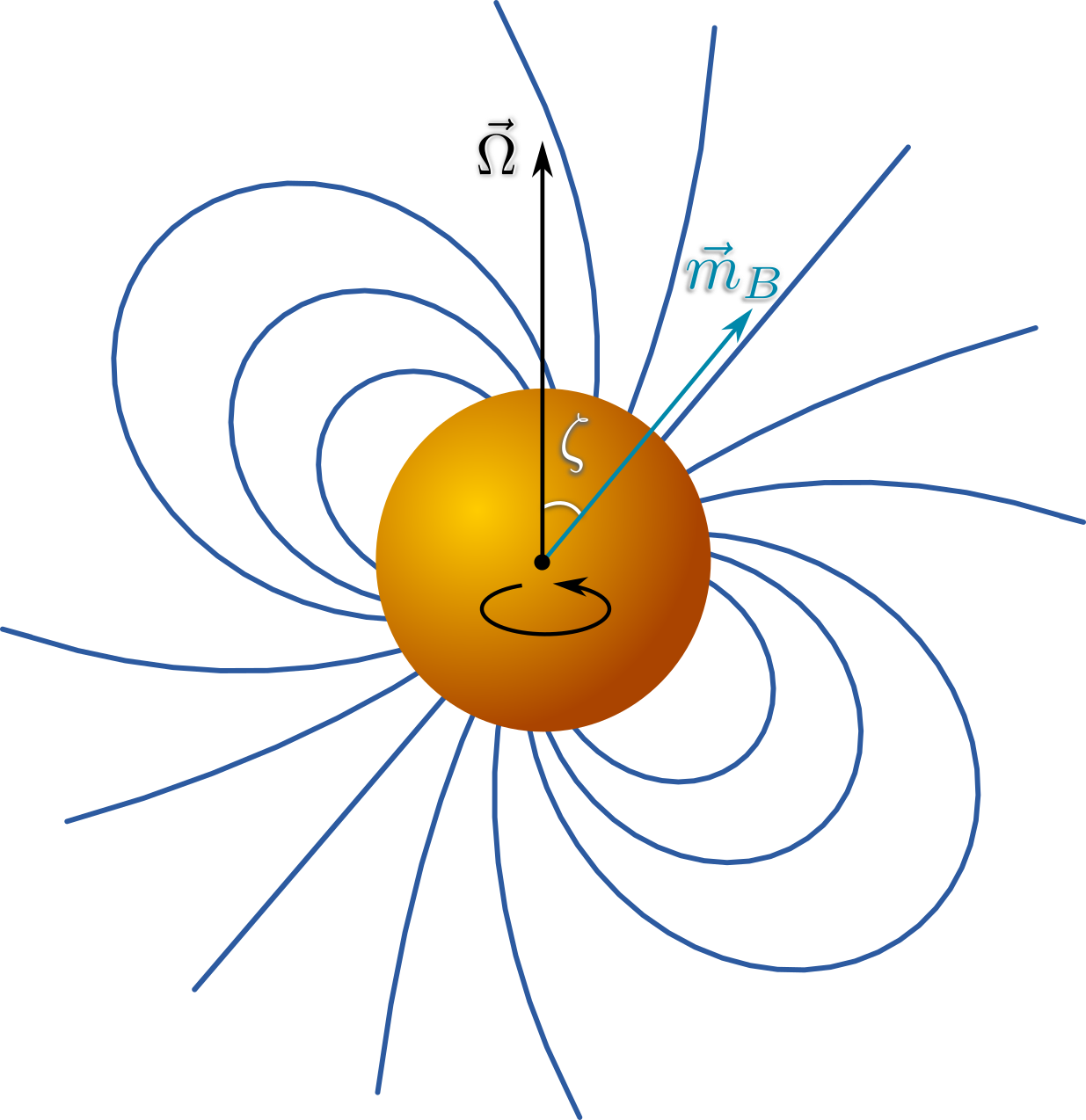
Figure 1: An oblique magnetic rotator. The photosphere is orange, the vertical rotation axis is shown in black, with the angular velocity ${\vec{\Omega}}$ along the $z-$axis. The magnetic dipole axis ${\vec{m}_{B}}$ is shown in blue with the initially dipolar field lines. The magnetic tilt angle is $\zeta$.

In this work, our aim is to extend this modeling effort using the Riemann Geomesh MHD code (Balsara et al., 2019; Florinski et al., 2020). Rather than using a conventional spherical $(r,\theta,\phi)$ grid, Riemann Geomesh employs a recursive partitioning of the spherical icosahedron based triangular meshing of the sphere, and a non-linear radial grid to map the volume of the wind, typically out to $10-20R_{\star}$. The resultant mesh maps the surface of the sphere as uniformly as possible, which traditional Cartesian based meshing is unable to accomplish, especially near the rotational poles. The Riemann Geomesh code is therefore uniquely suited to simulate oblique magnetic rotators in a bias free fashion.

The classification of centrifugal magnetosphere (CM) and dynamical magnetosphere (DM) is based on an aligned magnetic rotator, as displayed in Figures 2a and 2c. This system of classifying magnetospheres is especially relevant to aligned magnetic rotators but including a tilt angle complicates this simple classification scheme, as can be seen in Figures 2b and 2d. Figure 2b shows a tilted “dynamical” magnetosphere. Figures 2b and 2d are just conjectured sketches intended to sensitize the reader that the inclusion of three dimensionality introduces a third important parameter into our discussion; i.e. the tilt between the rotation axis and the dipole axis. A major aim of this work is to examine the dynamics of these magnetospheres in 3D to understand the role of magnetic tilt.

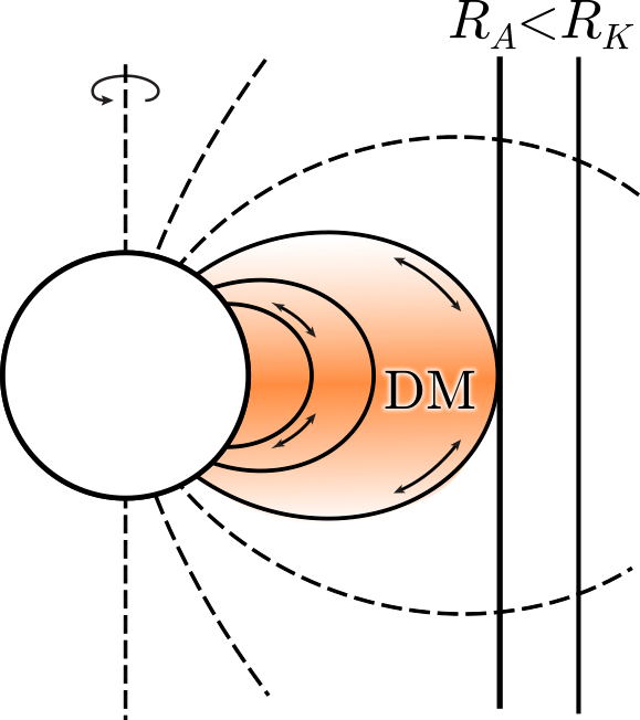
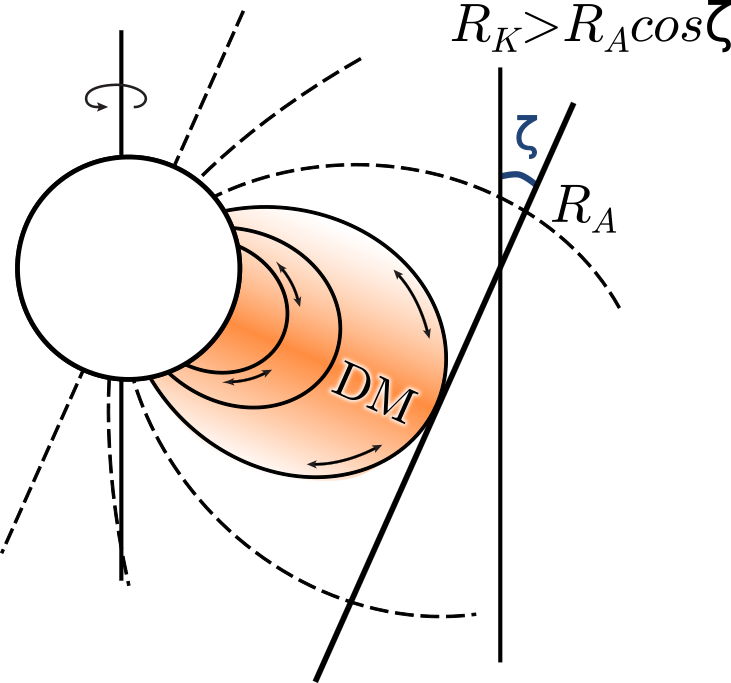
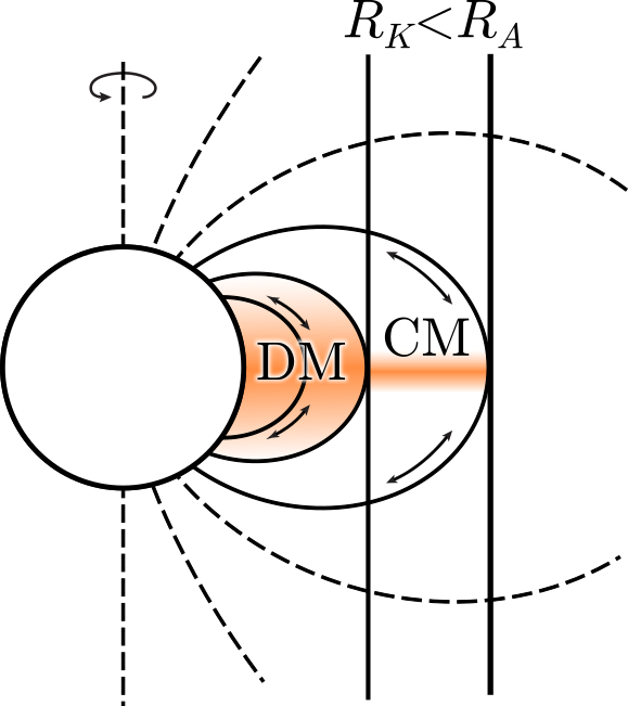
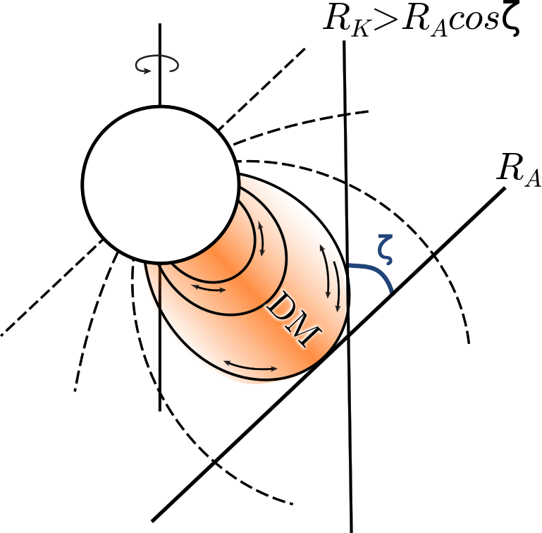
(a)                          (b)                                (c)                                 (d)

Figure 2: Schematic magnetosphere diagrams. (a) An aligned dynamical magnetosphere (DM): the Alfvén radius $R_{\rm A}$ is inside the Kepler corotation radius $R_{\rm K}$. Mass inside the magnetosphere (orange) will fall back onto the photosphere. (b) A sketch of a tilted DM with $R_{\rm A}<R_{\rm K}$. (c) An aligned centrifugal magnetosphere (CM): the Kepler corotation radius $R_{\rm K}$ is inside the Alfvén radius $R_{\rm A}$ (d) A conjectured sketch of a tilted magnetosphere (that would have been a CM if it were aligned). The tilt causes $R_{\rm A}cos\zeta<R_{\rm K}$ even if we initially had $R_{\rm K}<R_{\rm A}$. We caution that (b) and (d) are just conjectures at this point in the narrative. Figures (a) and (c) are adopted from Petit et al. (2013).

In this paper, we present and analyze 3D simulations of magnetically channeled winds around oblique magnetic rotators. The first goal of this paper is to show that the geodesic mesh MHD code can perform accurate simulations with large tilt angles and rotation rates. The second goal of this paper is to examine the dependence of the quasi-steady state mass-loss rate with rotation, magnetic confinement, and magnetic tilt angle, and to test the prediction that the overall mass-loss rate should decrease with the magnetic field, and increase with the rotation rate (ud-Doula et al., 2009) . The third goal of this paper is to use the 3D simulations to look for and study the episodic breakout events which are predicted to occur in centrifugal magnetospheres (ud-Doula et al., 2006; Shultz et al., 2020). The corresponding angular momentum flux is also shown as a function of $\theta,\phi$ at the outer most boundary of the simulation. The fourth goal is to estimate spindown as the star loses mass and angular momentum over its lifetime. This is achieved with the help of mass flux and angular momentum flux obtained at the outer boundary of the simulation. ud-Doula et al. (2008) analyze angular momentum evolution and spindown for aligned magnetic rotators in 2D.

The outline of this paper is as follows: in section 2 we describe the geodesic mesh along with the value it provides for this work. In section 3 we describe the model, the boundary conditions, and the numerical simulations. In section 4 we present the quasi-steady state mass-loss rate for different magnetic tilt angles and rotation rates. In section 5 we show the episodic centrifugal breakout events in 3D, as well as the mass fallback close to the star. And in section 6 we plot angular momentum flux as a function of $\theta,\phi$, and show regions of high angular momentum flux, and estimate characteristic stellar spindown time. Lastly, in section 7 we present the summary and conclusion of this work.

2 Mesh and Methods

The overarching problem consists of simulating the magnetically channeled, line driven winds around rotating massive stars. Due to the spherical aspect of the problem, it is best to carry out the simulation on a mesh that is uniquely suited for this problem.

One of the innovative aspects of this paper is that we have carried out the simulations using a geodesic mesh, and imposed a globally divergence-free formulation of the MHD equations. The other major advance in the simulation of line driven winds is that the magnetic field is split into two components: one the curl free, background magnetic field ${\bf B_{0}}$ and the other being the time evolving component ${\bf B_{1}}$. This would be reflective of the fact that the primary source of the magnetic field i.e., the star itself, lies outside the simulation domain. The variations in the magnetic field due to the material outflow is modeled with the help of the evolving field ${\bf B_{1}}$. The simulations are carried out in the rotating frame of reference of the star. Consequently, the simulations include the forces that arise due to rotation, which are centrifugal and coriolis forces. The complete description of the MHD equations employed in this manuscript is provided in Appendix A. In Subsection 2.1 we describe the structure of the geodesic mesh. In Subsection 2.2 we explain why it is particularly useful for this problem.

2.1 Structure of the Geodesic Mesh

The simulation setup is comprised of a spherical domain around the star, discretised with uniform triangular patches using a spherical icosahedron as the base. The uniformity of such a geodesic mesh results in high accuracy and consistent time-steps, when compared to other meshing strategies Balsara et al. (2019); Florinski et al. (2020). In the following subsections, because of the novelty of the approach, the implementation of the meshing is described. Then the value of such a uniform mesh in a spherical domain is explained, in context with the simulation of a magnetized star.

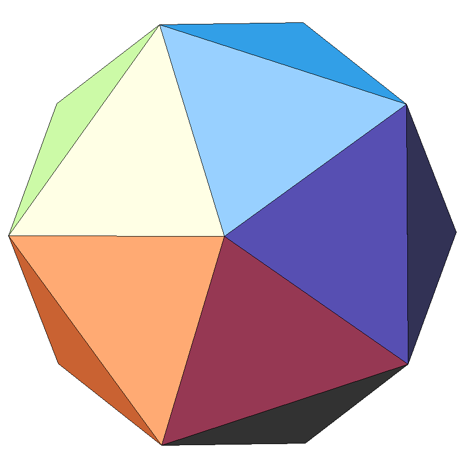
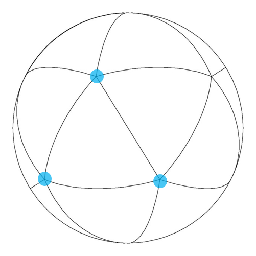
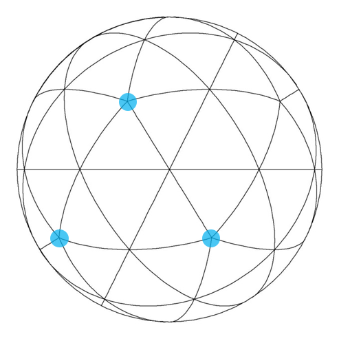
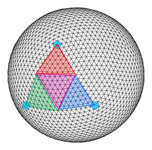
(a)                                 (b)                                  (c)                                 (d)

Figure 3: Icosahedron based spherical mesh: (a) a regular icosahedron Ruen & Bulatov (2012) (b) a spherical icosahedron, (c) first subdivision of the spherical icosahedron, and (d) fourth subdivision of the spherical icosahedron.

High accuracy MHD computations of spherical objects require a high quality meshing of the spherical domain. The traditional logically Cartesian based meshing of the sphere has two severe shortcomings: i) smaller zones at the poles lead to a shorter time-steps and ii) the geometric singularity causes a loss of accuracy at the poles. As a result, it is preferred to discretise the sphere by the structures emerging from the spherical icosahedron. Then recursive bisections of the geodesic curves can be used to obtain the required level of angular refinement shown in Figure 3.

The icosahedron shown in Figure 3a is used to obtain a spherical icosahedron shown in Figure 3b. The first subdivision of the spherical icosahedron is illustrated in Figure 3c, continuing this subdivision three more times, we get finer discretisation of the icosahedron-based spherical mesh, shown in Figure 3d. The colored patches in Figure 3d suggest that such a mesh structure leads naturally to large-scale numerical parallelisation. We exploit the symmetry and the divisibility of the geodesic mesh to perform these simulations efficiently on thousands of compute cores.

The discretisation shown in Figure 3b is referred to as level-0 sectorial division. It consists of 20 great triangles that subtend an angle of $\pi/2-\tan^{-1}(1/2){\rm rad}\approx 63.4^{\circ}$ from the center of the sphere. The first subdivision shown in Figure 3c is referred to as level-1 discretisation, with 80 great triangles, each subtending an average angle of $33.9\arcdeg$. Each colored triangle in Figure 3d therefore represents a level-1 sector. In the same way, the level-4 discretisation depicted in Figure 3d subtends an angle of $\approx 4.33\arcdeg$. While it is difficult to display the level-5 subdivision, it yields an angular resolution of $2.16\arcdeg$. At this angular resolution, the simulations in this study cover the spherical surface with $20,480$ spherical triangles.

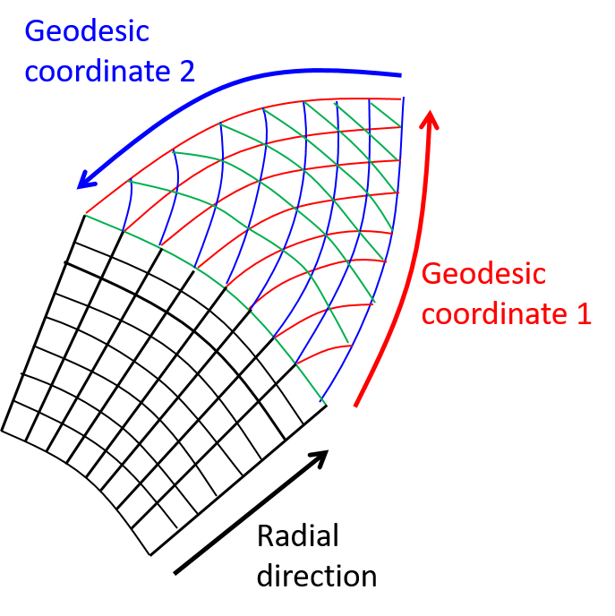
Figure 4: Discretisation along the radial direction and numbering strategy for the triangulation.

Due to the fast changing nature of the CAK velocity and density profiles, it is essential to have a very thin radial discretisation close to the star: $\Delta r=1.0\times 10^{-3}R_{\star}$ or slightly larger. This way, the thin radial zones near the photosphere initially expand geometrically, and then expand logarithmically out to 15 stellar radii. The 3D mesh is formed by extruding the 2D mesh with 240 radial zones. The mesh volume is therefore divided into $240\times 20,480\approx 5.0\times 10^{6}$ zones. The geodesic coordinates 1 and 2 in Figure 4 are shown in red and blue. With the radial coordinate (in black) they define access to each zone on the geodesic mesh.

2.2 Value of Geomesh

Our geodesic-based mapping of the sphere does not have any preferred orientation, it is highly regular and uniform in the angular direction. While a logically rectangular mesh in $(r,\theta,\phi)$ coordinates has singularities at the poles. The drawbacks of coordinate singularities include, but are not limited to, i) difficulty in doing constrained transport at the poles and ii) reduction in time-step and accuracy of the solution at the poles, Balsara et al. (2019). It has also been reported in Daley-Yates et al. (2019) that there can be fictitious heating of gas at the poles. The mesh shown in Figure 3 is free of such singularities. Since such a mapping is uniform, a general case of magnetic rotation can be described by choosing a fixed axis for the rotation, and only varying the orientation of the magnetic field. Also, the Geomesh code employs state-of-the-art Multidimensional Riemann solvers and a WENO-AO scheme, which are specifically developed for unstructured meshes (Balsara & Dumbser, 2015; Balsara et al., 2020). The divergence free evolution of magnetic field $\nabla\cdot{\bf B_{1}}=0$ is enforced with the help of Yee-type collocation of facially averaged magnetic fields. This along with the edge-integrated electric fields, achieve a high-order accurate numerical implementation of Faraday’s law; which ensures a divergence free evolution of magnetic field Balsara et al. (2019). Please see a recent review by Balsara (2017) for a detailed explanation of these computational techniques, as they apply to astrophysical MHD simulations.

In this work, the rotation axis of the star is chosen to be $z$-axis and the orientation of the dipole magnetic field is setup with respect to the $z$-axis. The simulations are carried out for different tilt angles ($\zeta$), such as 0, 45, 75 degrees of angular separation between the $z$-axis and the magnetic dipole axis. The next section provides the explanation for modeling of the massive star wind and the boundary conditions used.

3 Modeling and Boundary Conditions

The schematic of the simulation setup is shown in Figure 1. The radius of the stellar surface $R_{\star}$ is taken as the inner boundary and the outer boundary $R_{\rm o}$ is chosen as $15R_{\star}$. The dipolar magnetic field is maintained throughout the simulation domain by means of the background magnetic field ${\bf B_{0}}$. The magnetic flux density is parametrized by $\eta_{\star}$ (see Eq. 1).

3.1 Initial Conditions

Our template star is the O4 I(n)fp supergiant $\zeta$ Puppis. Specifically, we use the spherical parameters derived by Howarth & van Leeuwen (2019) based on the Hipparcos distance $d=332\pm 11$ pc: $L_{\star}=4.47\times 10^{5}L_{\odot},T_{\rm eff}=40\,000\,{\rm K},R=13.5R_{\star},M=25M_{\odot}$, and $\dot{M}\approx 1.5\times 10^{-6}M_{\odot}\,{\rm yr}^{-1}$. $\Gamma_{\rm e}=0.471$ is the Eddington parameter for $\zeta$ Pup. In the case of spherically symmetric mass loss, the CAK mass loss rate is given by, (Owocki, 2004),

$${\dot{M}}_{\rm CAK}=\dfrac{L_{\star}}{c^{2}}\dfrac{\alpha}{(1-\alpha)(1+\alpha)^{1/\alpha}}\left(\dfrac{\bar{Q}\Gamma_{\rm e}}{1-\Gamma_{\rm e}}\right)^{(1-\alpha)/\alpha}$$ (5)

where, $\alpha$ is the CAK exponent (Castor et al., 1975), $L_{\star}$ is the stellar bolometric luminosity, $\bar{Q}$ is the quality of the resonant absorption and $c$ is the speed of the light. We initialize our model with a spherically symmetric wind with standard $\beta$-law. The radial velocity along the radial-$r$ direction is given by,

$$v(r)=v_{\infty}\left(1-\dfrac{R_{\star}}{r}\right)^{\beta}$$ (6)

where, $v_{\infty}$ is the terminal wind speed, and $\beta$ is the velocity exponent. The terminal velocity speed is assumed to be $3$ times the escape velocity, $v_{\infty}=3v_{\rm esc}$ and the $\beta=0.8$ (Friend & Abbott, 1986; Owocki, 2004). The density is initialized using the mass-loss rate and the velocity,

$$\rho(r)=\dfrac{{\dot{M}}_{\rm CAK}}{4\pi r^{2}v(r)}$$ (7)

3.2 Boundary conditions

Owing to the rapidly changing velocity and density profiles of the CAK wind, it was essential to do a resolution study with different $\Delta r$ values close to star. For this, three different values of $\Delta r=1.0\times 10^{-3}R_{\star}$, $3.0\times 10^{-3}R_{\star}$ and $5.0\times 10^{-3}R_{\star}$ were chosen. The resulting density and velocity profiles from these simulations matched each other well, producing the expected mass loss rate ${\dot{M}}$. Hence, as mentioned earlier the discretisation close to the star has $\Delta r\approx 1.0\times 10^{-3}R_{\star}$.

At the inner boundary ghost zones, following ud-Doula & Owocki (2002b), we set the radial velocity by constant-slope extrapolation and fix the density at a value $\rho_{\rm c}$ chosen to ensure subsonic base outflow for the characteristic mass flux of a one-dimensional, nonmagnetic CAK model, i.e., $\rho_{\rm c}=\dot{M}/{4\pi R_{\star}^{2}a}/15$. The evolving magnetic field component ${\bf B_{1}}$ (see Appendix A) is initialized to zero at the inner boundary. At the outer boundary, far from the star, standard outflow conditions are maintained.

In the case of line driven winds, the acceleration just above the photosphere is high. Consequently, the density declines rapidly, while maintaining a quasi-steady mass-loss rate Owocki (2004). In order to numerically account for the steep density gradient, the zones near the inner boundary are very thin in the radial direction, increasing geometrically out to $1.5R_{\star}$, and increasing logarithmically at larger radii. A heuristic factor $k_{\rho}$ is applied at the inner radial boundary, such that $\rho_{\ast}=k_{\rho}\rho_{\rm sp}$, where $\rho_{\rm sp}$ is the estimated sonic-point density.

The value of $k_{\rho}$ is taken to be $15$ and it can be seen in Table 1 of section 4 that the simulated mass-loss rate matches within $5\%$ of the theoretical mass-loss rate, which is $1.43\times 10^{-6}M_{\odot}/{\rm yr}$. In the next subsection CAK acceleration source terms are described.

3.3 Source terms

The basic formalism for the acceleration of line driven winds was developed by Castor, Abbott and Klein in 1975 (CAK) (Castor et al., 1975). The one-dimensional CAK line acceleration along the radial direction $r$ is given by,

$$g_{\rm CAK}=\frac{f_{\rm d}}{1-\alpha}\frac{\kappa_{\rm e}L_{\star}\bar{Q}}{4\pi r^{2}c}\left(\frac{dv/dr}{\rho c{\bar{Q}}\kappa_{\rm e}}\right)^{\alpha}$$ (8)

where, $f_{\rm d}$ is a finite disk correction factor, which accounts for the solid angle of the photosphere. The remaining terms represent the CAK line force from a luminous point source. $\kappa_{\rm e}$ is the opacity due to free electrons, and $v$ is the velocity. There are two additional implicit acceleration terms: i) the radial gravitational acceleration $g_{\rm grav}$ and ii) accelerations induced by the rotating reference frame of the simulation, namely, the Coriolis and centrifugal accelerations ${\bf g}_{\rm rot}$. Therefore, the total acceleration is:

$${\bf g}_{\rm tot}=g_{\rm CAK}{\bf{\hat{r}}}+g_{\rm grav}{\bf{\hat{r}}}+{\bf g}_{\rm rot}$$ (9)

The expressions for the gravitational and rotational accelerations are provided in Appendix A, along with the complete set of MHD equations. The simulations are performed using these initial and boundary conditions and the source terms for a range of magnetic confinement parameters $\eta_{\star}$, magnetic tilt angles $\zeta$, and critical rotation ratios $W$. The next section describes the simulations, and the transition from initial conditions to quasi-steady state behavior.

4 Transition to Quasi-steady State

The 3D Riemann Geomesh simulations described here span a range of magnetic tilt angles $\zeta=0,45\arcdeg,75\arcdeg$, two rotation rates $W=0,0.5$, and three magnetic confinement parameters, $\eta_{\star}=0,10,50.$ The ten cases are listed in Table 1, with the corresponding Kepler and Alfvén radii, and the corresponding aligned-magnetosphere classification: CM for centrifugal magnetospheres, and DM for dynamical magnetospheres. The outgoing mass-loss rates in the last column are discussed below.

Table 1: Quasi-steady-state mass-loss rates as a function of magnetic confinement $\eta_{\star}$, magnetic tilt angle $\zeta$, and critical rotation ratio $W$. $R_{\rm A}$ and $R_{\rm K}$ are the corresponding Alfvén and Kepler radii in stellar radius $R_{\star}$. CM indicates a centrifugal magnetosphere, for which $R_{\rm A}>R_{\rm K}$. DM indicates a dynamical magnetosphere, for which $R_{\rm A}\leq R_{\rm K}$. ${\dot{M}}$ is the time-averaged mass-loss rate out of the outer boundary in solar masses per year.

$\eta_{\star}$	$\zeta$	$W$	$R_{\rm K}$	$R_{\rm A}$	CM/DM	${\dot{M}}$
			$(R_{\star})$			($M_{\odot}/{\rm yr}$)
0	$0\arcdeg$	0	$\infty$	-	-	1.49 $\times 10^{-6}$
0	$0\arcdeg$	0.5	1.59	-	-	1.70 $\times 10^{-6}$
10	$0\arcdeg$	0	$\infty$	2.1	DM	6.92 $\times 10^{-7}$
10	$0\arcdeg$	0.5	1.59	2.1	CM	8.37 $\times 10^{-7}$
10	$45\arcdeg$	0.5	1.59	2.1	CM	7.96 $\times 10^{-7}$
10	$75\arcdeg$	0.5	1.59	2.1	CM	5.88 $\times 10^{-7}$
50	$0\arcdeg$	0	$\infty$	2.9	DM	4.35 $\times 10^{-7}$
50	$0\arcdeg$	0.5	1.59	2.9	CM	4.58 $\times 10^{-7}$
50	$45\arcdeg$	0.5	1.59	2.9	CM	5.84 $\times 10^{-7}$
50	$75\arcdeg$	0.5	1.59	2.9	CM	4.41 $\times 10^{-7}$

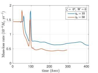
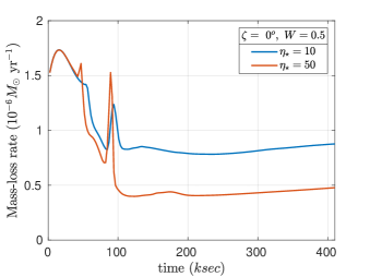
(a)                                                                     (b)

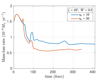
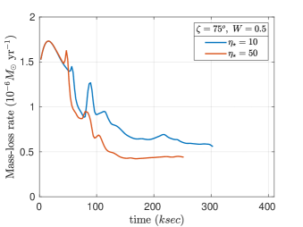
(c)                                                                     (d)

Figure 5: Mass-loss rate at the outer boundary as a function of time showing the approach to quasi-steady state. Shown in red (lower curve) $\eta_{\star}=10$, and in blue (upper curve) $\eta_{\star}50$ for: (a) $\zeta$ = $0\arcdeg$, $W=0$, (b) $\zeta$ = $0\arcdeg$, $W=0.5$, (c) $\zeta$ = $45\arcdeg$, $W=0.5$, and (d) $\zeta$ = $75\arcdeg$, $W=0.5.$ Quasi-steady state is achieved typically after $\approx 110$ ks.

We first note that although we do not include our simulations at $W=0.25$, the behavior of the DMs can be seen in the $W=0$ simulations. Second, we did not consider $W>0.5$ because at very high rotation the photosphere becomes oblate (ud-Doula et al., 2008), and the spherical mesh is no longer appropriate. Third, we note that higher values of $\eta_{\star}$ lead to significantly longer compute times. High magnetic confinement simulations will be the subject of a future paper.

Figure 5 shows the integrated mass loss from the outer boundary of the simulation as a function of time. The figures show the mass-loss rate reaching a quasi-steady value after $100-120$ ksec. The mass-loss spikes seen in all simulations are the initial mass blow out, which occurs as the initially dense inner CAK wind exits the outer boundary.

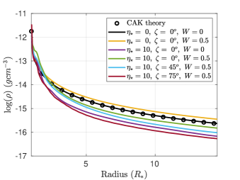
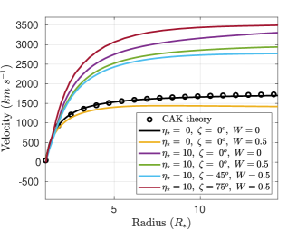
(a)                                                                     (b)

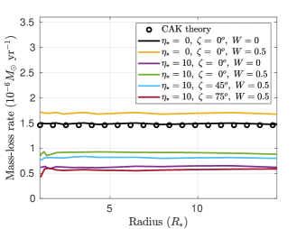
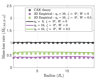
(c)                                                                     (d)

Figure 6: Variation of (a) log density, (b) radial velocity and (c) mass-loss rate as a function of radial distance $R$. (d) mass-loss rate for the aligned cases in comparison with empirical formula derived in ud-Doula et al. (2008) The quantities are averaged over $\theta,\phi$ directions, for six sets of magnetic confinement $\eta_{\star}$, magnetic tilt angle $\zeta$ and critical rotation fraction $W$. The non-magnetic CAK mass-loss rate is shown with open circles.

In the first simulation with no magnetic field and no rotation, a steady state is reached quickly, and, reassuringly, the density, velocity and mass-loss profiles follow those predicted by CAK theory. These can be seen, respectively in Figures 6a, 6b and 6c as solid black lines (simulation) and black open circles (CAK theory). In the second simulation, rapid rotation is accounted for by means of centrifugal and Coriolis forces, as described in Appendix A. These forces act perpendicular to the $z$ rotation axis and tend to increase density and mass-loss rate, but decrease radial velocity, approaching the rotational equator in the $xy$-plane. Averaged over $\theta,\phi$, this can be seen as the yellow solid radial profiles in Figs. 6a-c. The $\sim 15\%$ increase in the mass loss rate, averaged over $\theta,\phi$ at the outer boundary, can be seen in the last column of Table 1, and is similar to the 2D simulation results obtained by ud-Doula et al. (2008). In the absence of a magnetic field, the increase in $\dot{M}$ is accompanied by an average decrease in $v_{\infty}$. This can be understood as a decrease in the escape velocity $v_{\rm esc}$ with increased rotation.

For the magnetic simulations with $\eta_{\star}=10,50$, $W=0,0.5$ and $\zeta=0\arcdeg,45\arcdeg,75\arcdeg$ (see Table 1) the initially dipolar field is stretched open near the magnetic poles, and remains closed near the magnetic equator, out to approximately the Alfvén radius, channeling wind material into the closed magnetosphere, thereby reducing the mass-loss rate at the outer boundary. The reduction in $\dot{M}$ is more pronounced for higher magnetic confinement, consistent with prior 2D results (ud-Doula et al., 2008). Table 1 also shows that, in all but one case ($\eta_{\star}=50$, $\zeta=75\arcdeg$), higher rotation leads to higher $\dot{M}$.

From Table 1 for $\eta_{\star}=10$, we see that as the tilt increases, the mass-loss rate is reduced. This behaviour suggests a dot-product $\cos\zeta$ variation involving the magnetic dipole moment ${\bf m_{B}}$ and the angular velocity ${\bf\Omega}$. That is, the moment arm of the mass outflow is reduced as tilt increases, thereby reducing the net mass-loss rate. The same is not true, however, at higher confinement, where the maximum $\dot{M}$ is achieved for $\zeta=45\arcdeg$.

In fact, the phenomenon depends upon the geometry of the tilt in addition to the competition between magnetic confinement and centrifugal forces. Therefore, a larger parameter study will be required to yield meaningful predictions. The complexity of the situation can be seen for $\eta_{\star}=50$, $W=0.5$ and $\zeta=45\arcdeg$, where the mass-loss rate is higher than both the $\zeta=0\arcdeg$ and $\zeta=75\arcdeg$ cases. Here we resort to the simulations to explain the situation. At high field $\eta_{\star}=50$, with no tilt $\zeta=0$, and rapid rotation $W=0.5$, much of the outflow close to the rotational equator is trapped in the magnetosphere. Because the centrifugal acceleration is greatest in the equatorial XY plane, $\dot{M}$ is not significantly increased by rapid rotation. This is evident in rows 7 and 8 of Table 1: the mass-loss rates at $W=0$ and $W=0.5$ are comparable. Examining Figure 9, with $W=0.5$, $\eta_{\star}=50$, and $\zeta=45\arcdeg$, most of the outflow near the rotational equator is along open field lines, thereby maximizing $\dot{M}$ and $\dot{J}$, the total rate of angular momentum loss. Figure 9 will be discussed in more detail in section 5. The total angular momentum loss is listed in Table 2 and discussed in section 6 below.

The Figure 6 shows the variation in log density, velocity and mass-loss rate as a function of radius at the end of each simulation. These are averaged over the $\theta,\phi$ to illustrate their radial variation. Outside the Alfvén radii, the mass-loss rate remains constant, while the density decreases rapidly and the velocity increases, as expected from CAK. In general, the presence of magnetic confinement $\eta_{\star}>1$ increases the overall radial velocity, while the density profile undergoes a reduction due to magnetic confinement. In the same way, in the presence of rotation, the density profile and the mass-loss rate increase, as the wind is flung out by rotational forces, consistent with prior 2D simulations (ud-Doula et al., 2008).

For the aligned rotator case, there is some well-developed theory for the mass loss case even when we have rotation and magnetic fields. We compare our simulations for aligned rotators with that theory in this paragraph. In figure 6d, the mass-loss rate for aligned magnetic field cases are presented. The mass-loss rate is normalized with respect to the non-magnetic and no-rotation case ($\dot{M}_{B=0}$). The green and purple circles in the plot are obtained from the analytic formula provided in equations 23 and 24 of ud-Doula et al. (2008) and repeated here as:

$$\dfrac{\dot{M}_{B}}{\dot{M}_{B=0}}\approx 1-\sqrt{1-R_{*}/R_{c}}$$

$$\dfrac{\dot{M}_{B}}{\dot{M}_{B=0}}\approx 1-\sqrt{1-R_{*}/R_{c}}+1-\sqrt{1-0.5R_{*}/R_{K}}$$

where, $R_{c}$ is the confinement radius of the magnetic closed loops. From our simulation results the confinement radius is observed to be of the form, $R_{c}\approx R_{*}+0.6(R_{A}-R_{*})$. We see from figure 6d that the agreement between our simulations and the theory is quite good. In the quasi-steady state, the simulations show the magnetic confinement of the wind and the episodic breakout events at the magnetic equator. This is detailed in section 5 below.

5 The Dynamics of Magnetic Channeling in the Wind

The mass outflow from the surface of the star is free to flow at the magnetic poles and it is confined near the equatorial region by the closed loops of the magnetic dipole field. Due to this, the wind coming from the either side of the equatorial region, guided by the magnetic field lines, meet and cause a field lines breaking at the magnetic equator. This overall behaviour of closed magnetic loops near the surface of the star and open field lines as we move farther can be seen in figures 7.

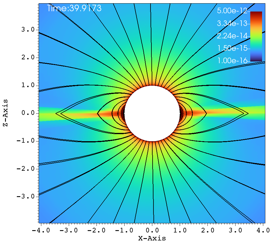
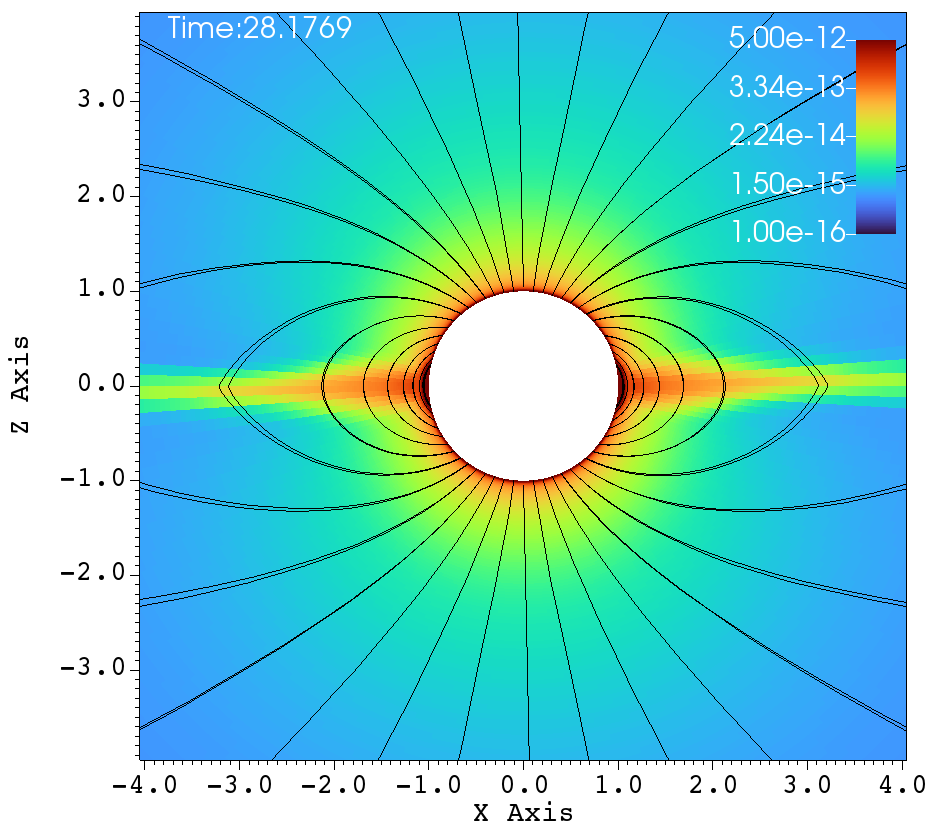
(a)                                                                   (b)

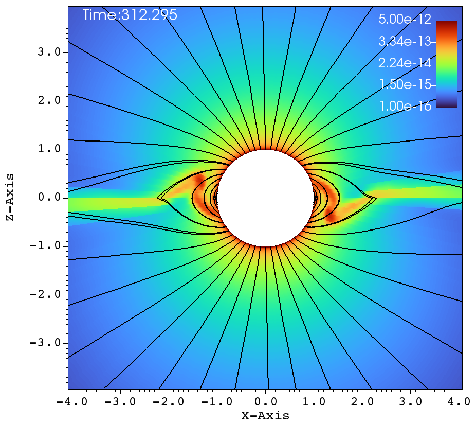
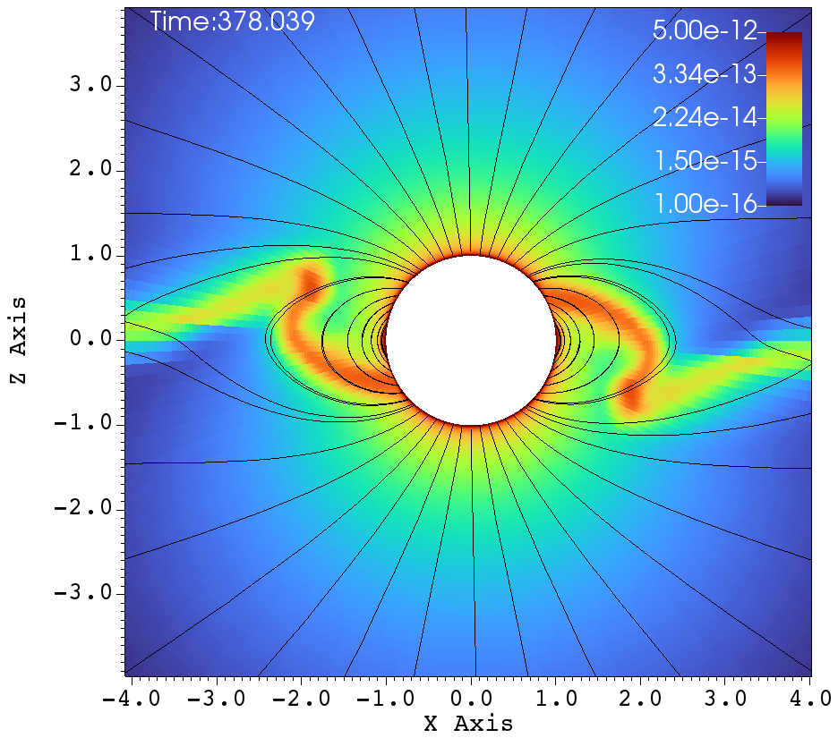
(c)                                                                   (d)

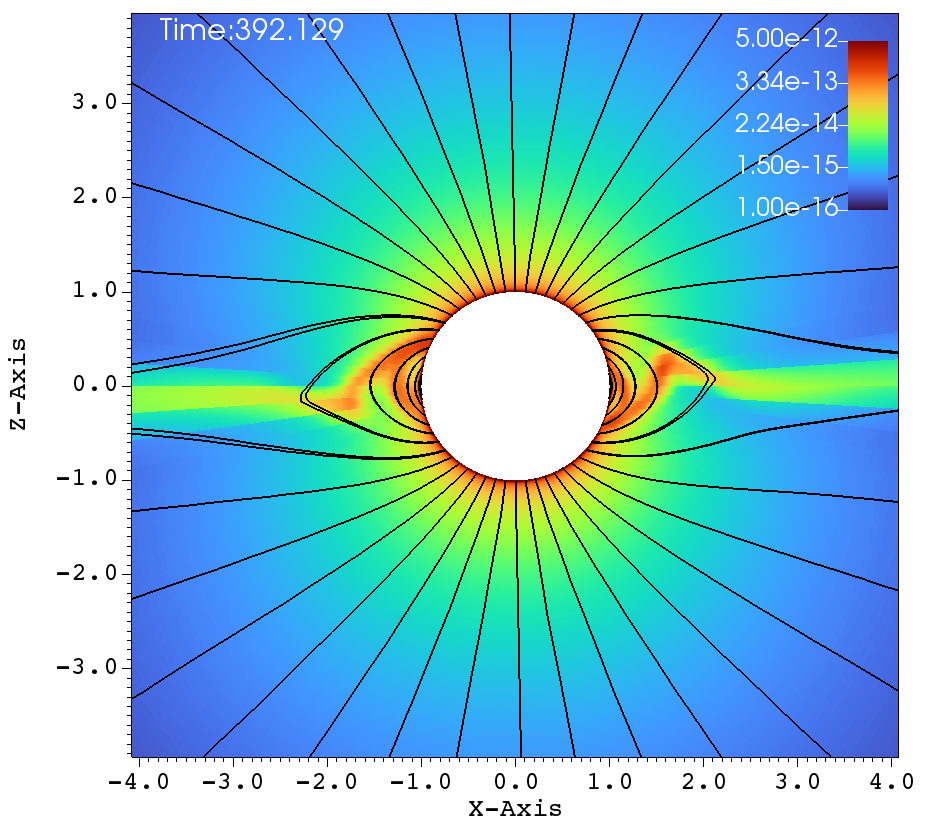
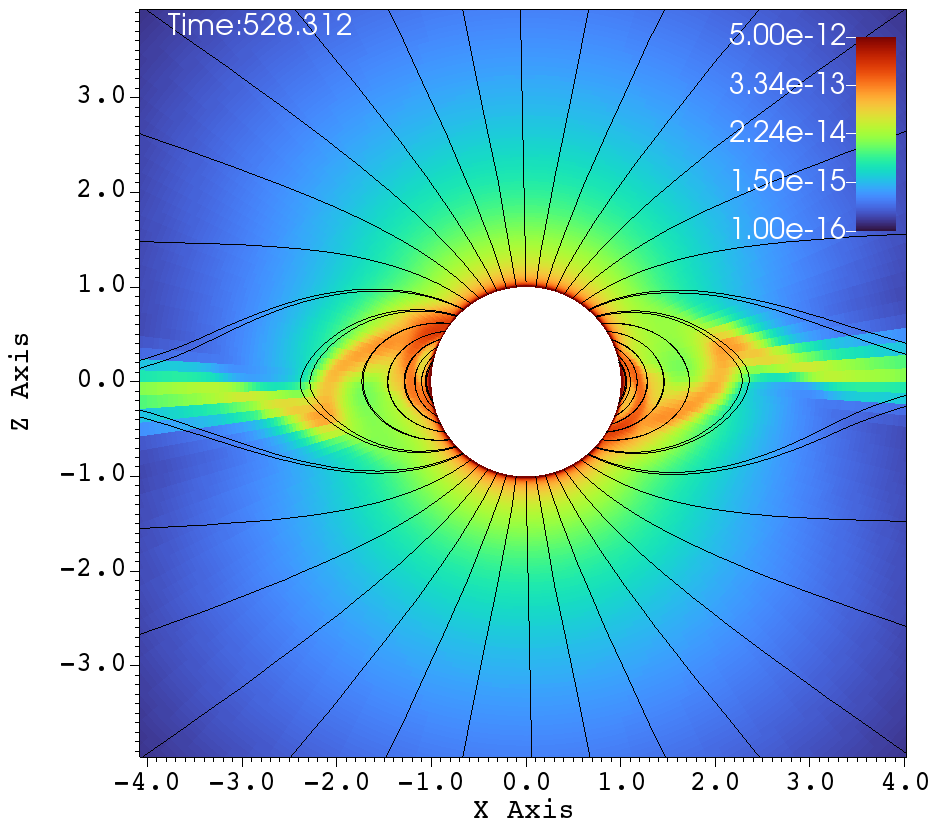
(e)                                                                   (f)

Figure 7: Density ($\rm g~{}cm^{-3}$) colorized with the magnetic field lines, at different times (ksec) of the simulation, for the case of $\eta_{\star}=10$ (a,c,e) and $\eta_{\star}=50$ (b,d,f), no rotation, showing the magnetic confinement and episodic outflow. The $x$ and $z$ axes values are in the scale of stellar radius $R_{\star}$.

Figures 7a-f shows the density colorized with the magnetic field lines at different times of the simulation, for the cases of magnetic field strength $\eta_{\star}=10,50$ and no rotation. These figures show the expected dynamics of a magnetically channeled line driven wind. We see that each closed loop has two foot-points that connect to the star at similar moment arms. Owing to the radially outward line driving force, both foot-points have similar amounts of matter that is driven out from the surface of the star. Because Figs. 7a, b, c correspond to a smaller magnetic field than Figs 7d, e, f, we can clearly see that the former set of figures produce a smaller magnetosphere than the latter set of figures.

The matter driven out from the either side of the star meet at the equatorial region, forming a dense knot. The knot is at a much higher density than the rest of the wind, and hence experiences a greater gravitational attraction towards the surface of the star. However, the closed field lines just below the knot prevents the direct fallback of matter on to the star and hence the path of the density knot fallback is dictated by the magnetic field lines. This can be seen in figures 7c, d. These observations are inline with the 2D simulations of ud-Doula & Owocki (2002b). In addition, in this 3D simulation, it can be seen that the density knots at the either end of the magnetic equator fallback from the opposite sides of the field lines, thereby conserving the momentum of the star (figures 7c-f). Also, the overall outflow is guided by the magnetic field lines from the either sides of the pole, in an alternate fashion and hence the subsequent density fallbacks come from the either side of the magnetic equator. This is also inline with the observations made in ud-Doula & Owocki (2002b).

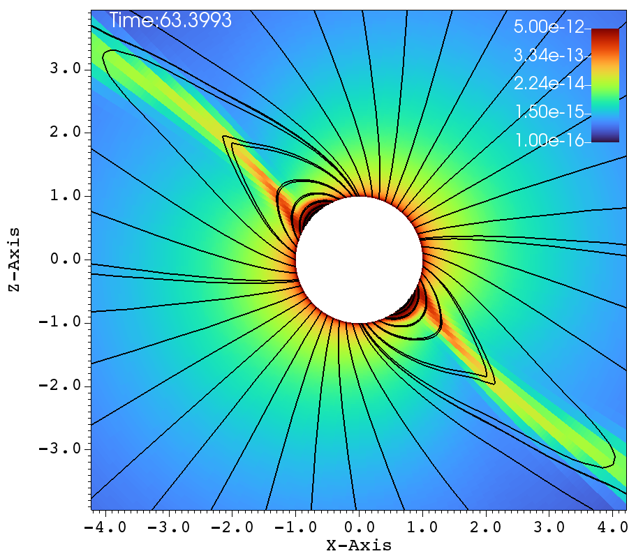
(a)                                                                   (b)

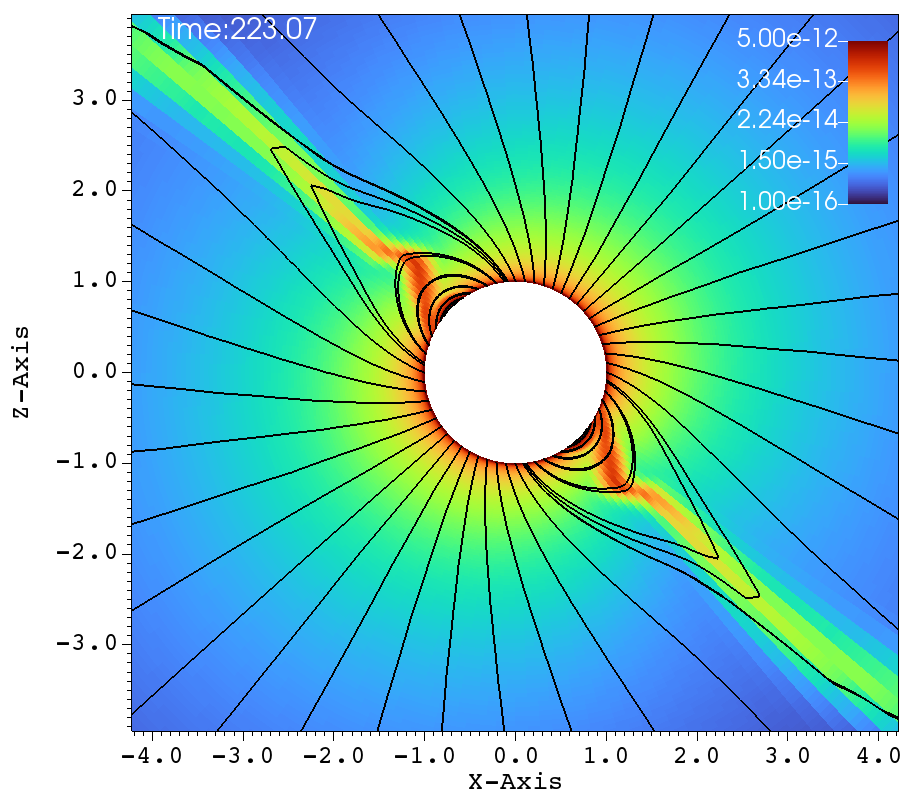
(c)                                                                   (d)

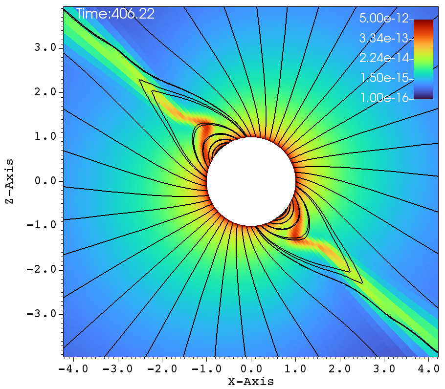
(e)                                                                   (f)

Figure 8: Density ($\rm g~{}cm^{-3}$) colorized with the magnetic field lines, at different times (ksec) of the simulation, for the case of $45\arcdeg$ tilted magnetic dipole with $\eta_{\star}=10$ and with the rotation of $W=0.5$, showing the magnetic confinement and the centrifugal pull due to the rotation. The $x$ and $z$ axes values are in the scale of stellar radius $R_{\star}$.

The next set of figures 8a-f, represent the simulations carried out with the high rotation and an inclined magnetic dipole. The magnetic field has the strength of $\eta_{\star}=10$ and the rotation rate is $W=0.5$, the rotation axis is the $z-$axis and the magnetic dipole makes a $\zeta=45\arcdeg$ inclination with the rotation axis. The dynamics are different and interesting in Figure 8, when comparing to that of Figure 7. Due to the tilt and high rotation, the streams of gas that come off from the two foot-points of a closed magnetic loop experiences unequal amount of centrifugal force. The magnetic foot-point that is closer to the rotational equator has more centrifugal force and is flung out faster. The other magnetic foot-point that is closer to the pole, does not have centrifugal assist when being flung outwards. Therefore the streamer that comes off from the foot-point that is closer to the rotational-equator dominates and hence that one dominant streamer is doing the flailing. This is in contrast to the case of aligned rotation, where, there are two streamers at either sides of the magnetic equator that go back and forth.

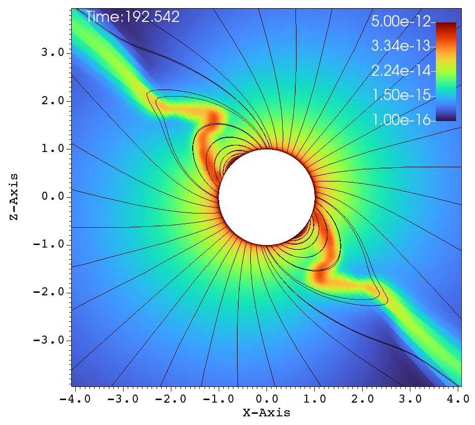
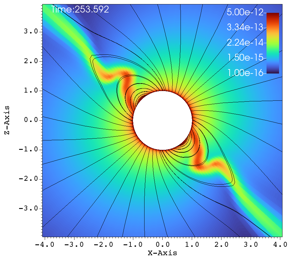
(a)                                                                   (b)

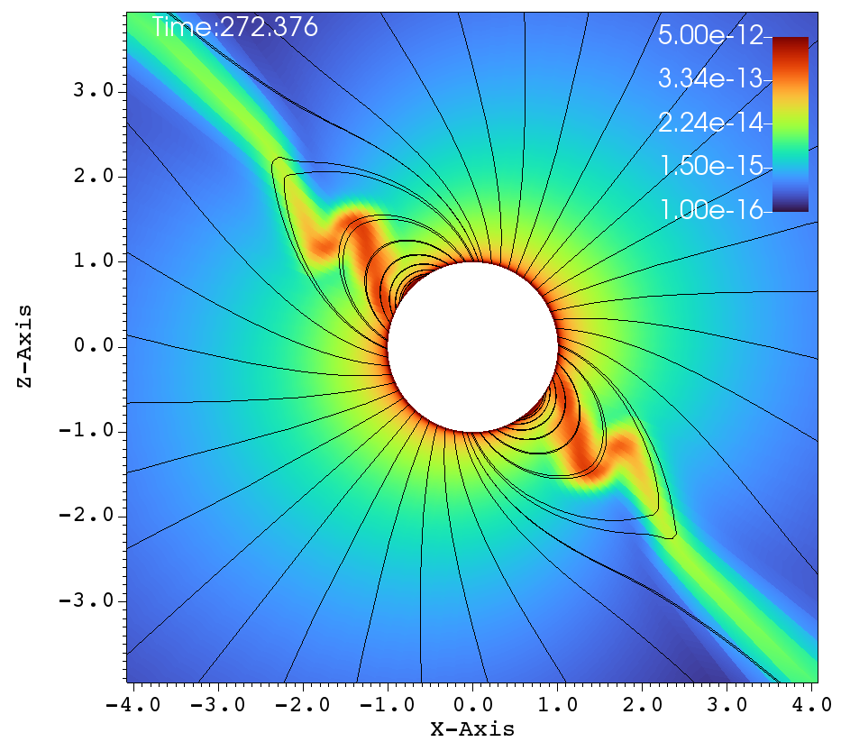
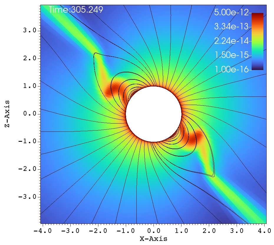
(c)                                                                   (d)

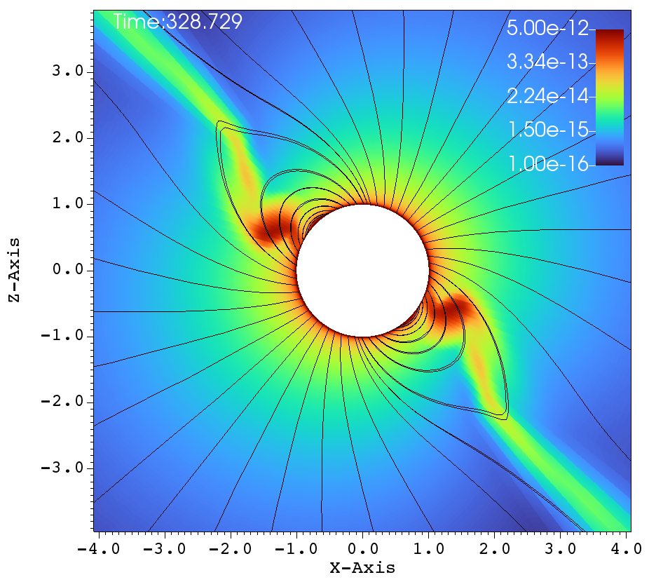
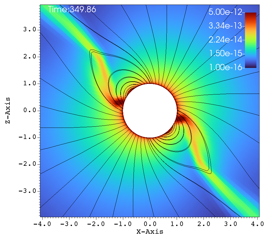
(e)                                                                   (f)

Figure 9: Density ($\rm g~{}cm^{-3}$) colorized with the magnetic field lines, at different times (ksec) of the simulation, for the case of $45\arcdeg$ tilted magnetic dipole with $\eta_{\star}=50$ and with the rotation of $W=0.5$. The $x$ and $z$ axes values are in the scale of stellar radius $R_{\star}$. While Figure 8 showed uniformly spread time intervals, this figure shows a set of snapshots that are bunched in time that reveal the filling of the magnetosphere and episodic in-fall of clumps. One entire episode from the start of clump formation to its in-fall is shown.

Similar lines of observations can be made for the figures 9a-f, that corresponds to $\eta_{\star}=50$, $W=0.5$, $\zeta=45\arcdeg$ case. In table 1, this case has $R_{A}=2.9$ and $R_{K}=1.59$ and it has been classified as a centrifugal magnetosphere (CM) based on the traditional explanations that have been developed so far. Upon observing the images at different times in Figure 9a-f, it can be seen that the magnetosphere successively filled and with clumps falling down on the star. This situation is similar to that of Figure 8a-f. Here, one would therefore be inclined to conclude that the simulation in Figure 9a-f is a dynamical magnetosphere (DM) even though it was classified as a CM. But a little reflection allows us to understand that $R_{A}$ should be modified by $cos\zeta$ so that $~{}R_{A}~{}cos\zeta\sim R_{K}$. Here, the tilt has brought the cosine-modified Alfven radius much closer to the Keplarian radius. This might explain two important features in Figure 9a-f. One, the clumps episodically keep filling the magnetosphere and falling back on to the star, similar to that of a dynamical magnetosphere case. Second, the majority of the magnetically streamlined mass outflow comes out from the magnetic foot point that is closer to the rotational-equator (xy-plane).

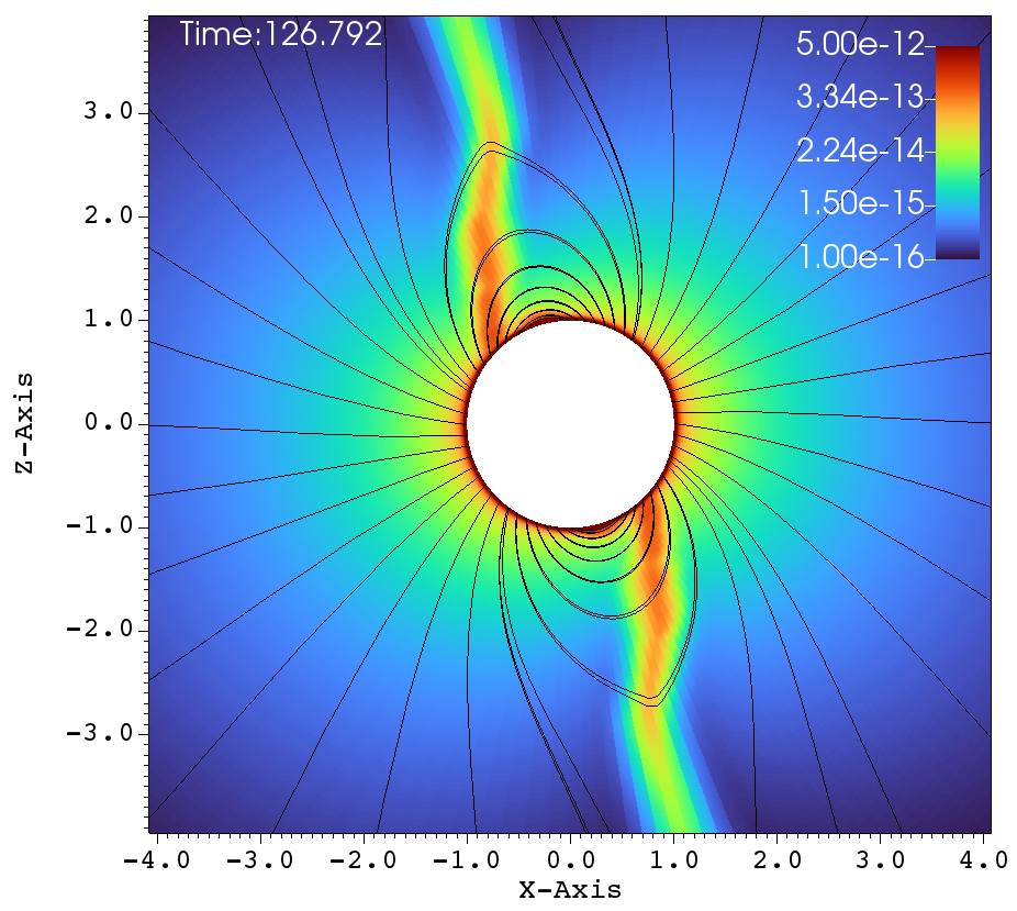
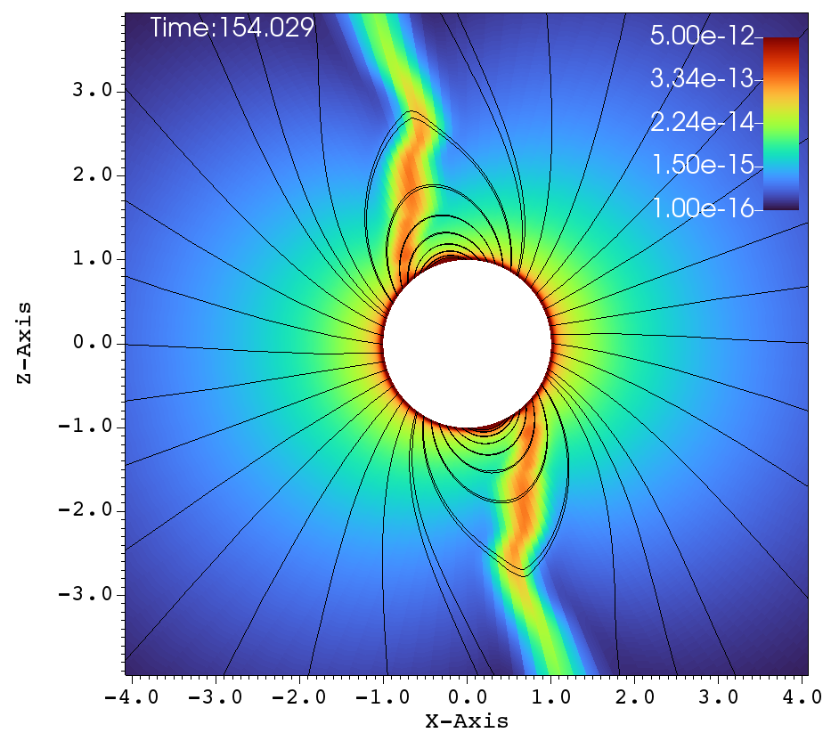
(a)                                                                   (b)

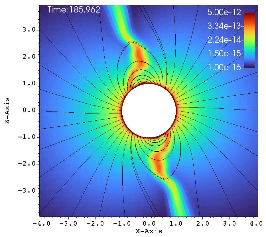
(c)                                                                   (d)

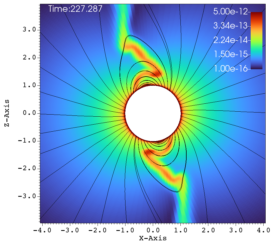
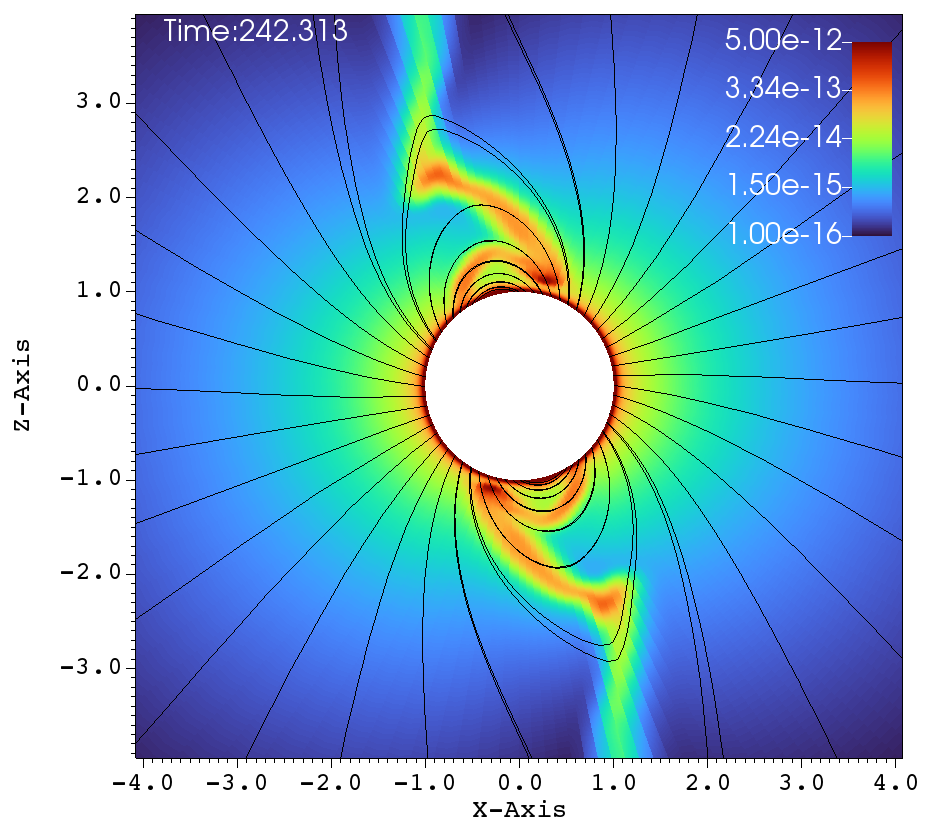
(e)                                                                   (f)

Figure 10: Density ($\rm g~{}cm^{-3}$) colorized with the magnetic field lines, at different times (ksec) of the simulation, for the case of $75\arcdeg$ tilted magnetic dipole with $\eta_{\star}=50$ and with the rotation of $W=0.5$. The $x$ and $z$ axes values are in the scale of stellar radius $R_{\star}$. While Figure 8 showed uniformly spread time intervals, this figure shows a set of snapshots that are bunched in time that reveal the filling of the magnetosphere and episodic in-fall of clumps. One entire episode from the start of clump formation to its in-fall is shown.

Figure 10 again shows one episode of the $\eta_{\star}=50$, $\zeta=75\arcdeg$ and $W=0.5$ simulation, as in Figure 9. We see one clump initiated in Figure 10a. Figures 10b-e show successive times when the clump is reined in by the magnetic field and in-falling material fills the magnetosphere. Figure 10f shows the precise moment when the clump impacts the star. Interestingly, at outer radii in Figure 10f we can see the start of another episode of clump initiation.

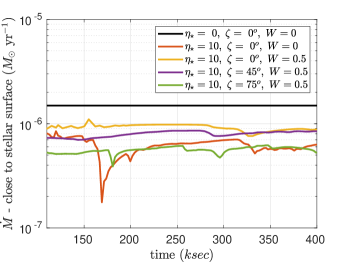
Figure 11: Observed mass-loss rate close to the stellar surface, at $R=1.1R_{\star}$, as a function of time (ksec), for different rotation rates and tilt angles. The clump formation and successfully falling back to the star happens for i) $\eta_{\star}=10,\zeta=0,W=0$ and ii) $\eta_{\star}=10,\zeta=75,W=0.5$ cases. The abrupt drops in the mass flow rate can be observed for the same two cases, showing the clumps falling back to the star.

The episodes of clump formation and fallback can also be seen, when observing the mass-loss rate close to the stellar surface. Referring to Figure 11, the mass-loss rate experiences abrupt drops for the cases, i) $\eta=10,\zeta=0,W=0$ and ii) $\eta=10,\zeta=75,W=0.5$, where the density knot is formed by one side of the stream and that knot proceeds to fall onto star on the other side of the magnetic loop. The other cases do not show such a complete fallback and hence they do not exhibit these sharp drops mass-loss rate close to the stellar surface.

In summary, the tilted dipole simulations shown in Figs. 8, 9 and 10 suggest that the tilt should be factored in when deciding whether we have a DM or CM. Larger simulated data sets will eventually enable us to identify the boundary between DM and CM in cases where the magnetic dipole has a large tilt relative to the rotational axis.

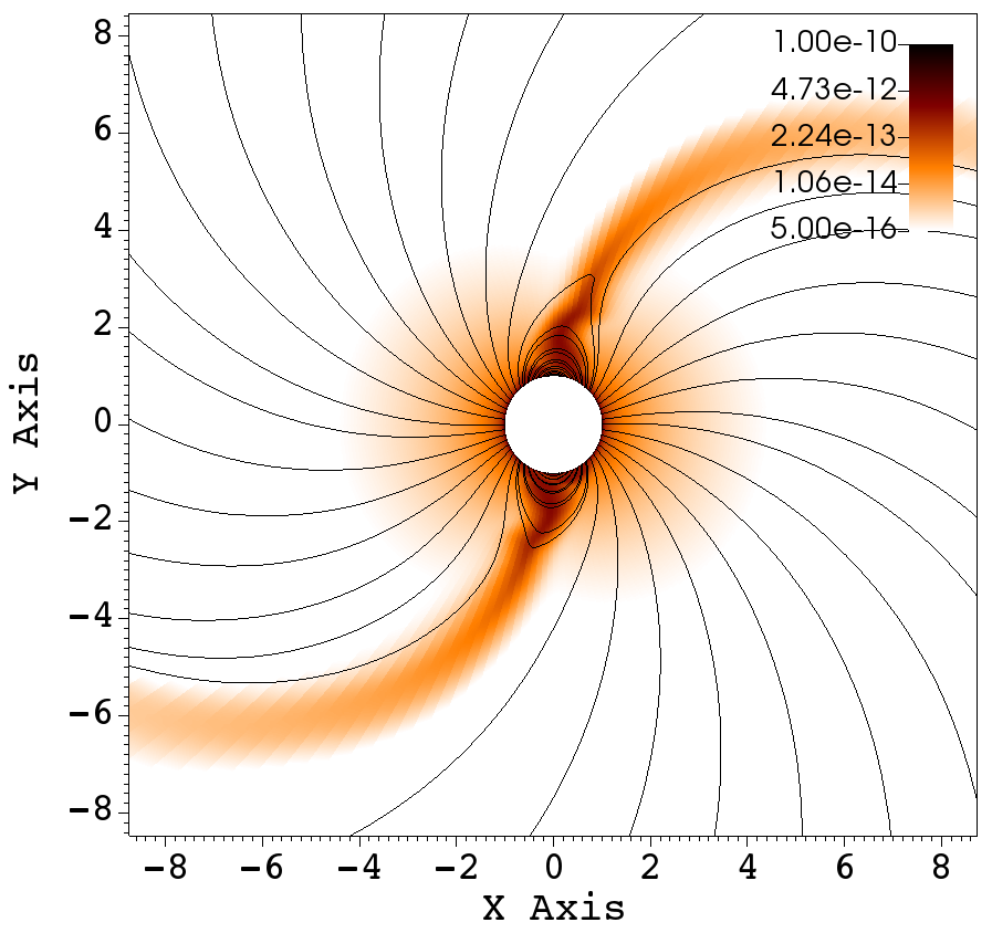
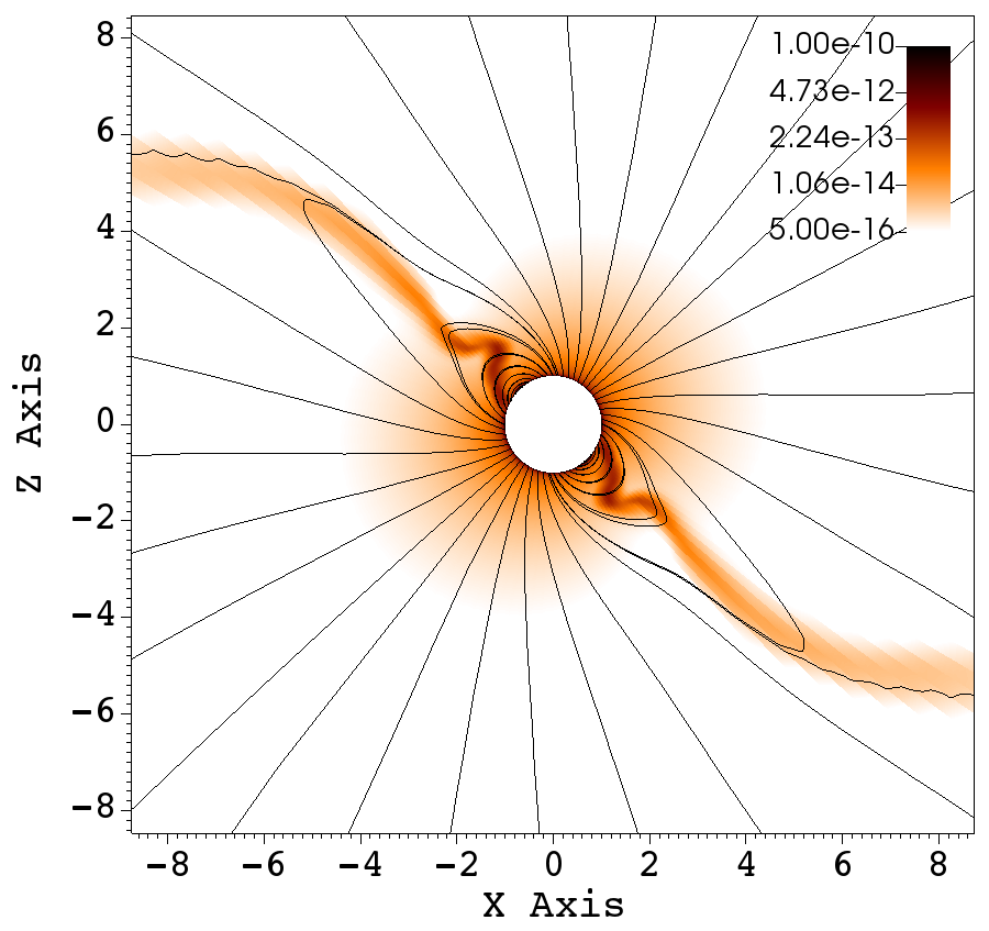
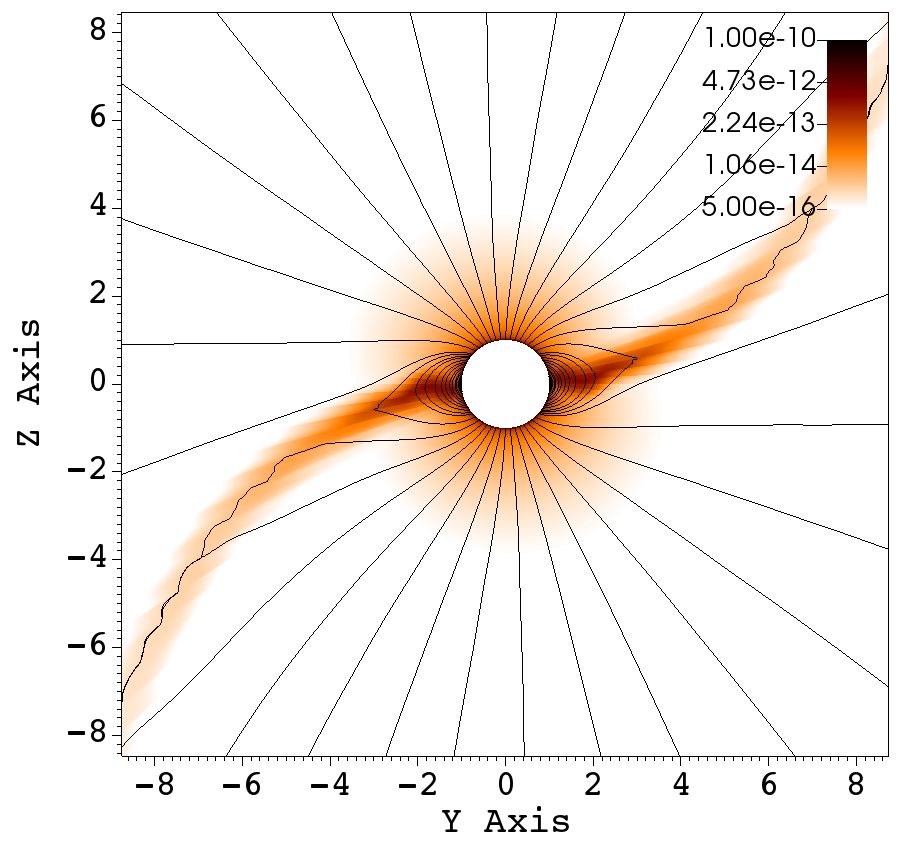
(a)                                               (b)                                              (c)

Figure 12: Density ($\rm g~{}cm^{-3}$) colorized with the magnetic stream lines along the XY, XZ and YZ planes at an intermediate simulation time of 240 ksec, for magnetic tilt $\zeta=45\arcdeg$, $\eta_{\star}=50$, and $W=0.5$.

All of the simulation results presented in this work have the rotation axis along the $z-$axis and the magnetic tilt oriented along the $xz-$plane. Owing to this, much of the interesting phenomena are best viewed in the $xz-$plane. In order to illustrate the 3D nature of the simulations, three cross sections are presented in Figure 12, where density and magnetic field lines are presented in the XY, XZ and YZ planes at an intermediate simulation time, for $\eta_{\star}=50$, $W=0.5$ and $\zeta=45\arcdeg$. In the next section, the angular momentum flux is described along with the calculation of mass loss rate and spin down time of the star.

6 Angular Momentum Loss Rate

Mass loss from rotating stars carries away angular momentum and leads to stellar spindown. In non-magnetic massive stars with line-driven winds, the mass-loss rate is large, but not enough to significantly increase their rotation periods during the main sequence because the angular momentum is only carried away by gas, and the main sequence lifetime is relatively short (e.g., Maeder & Meynet, 2000). In magnetic stars, most of the angular momentum is lost via the Poynting stress provided by the magnetic field, and not by the outflowing plasma itself (Weber & Davis, 1967; ud-Doula et al., 2009). Weber & Davis (1967) modeled the angular momentum loss of the Sun with the far-field approximation of a magnetic monopole. For stronger dipole fields, ud-Doula et al. (2009) showed that the angular momentum loss rate of an aligned magnetic rotator could be approximated as:

$${\dot{J}}_{\rm dWD}=\dfrac{2}{3}{\dot{M}}_{B=0}\Omega R_{\rm A}^{2},$$ (10)

where ${\dot{J}}_{\rm dWD}$ is the total angular momentum loss rate in the dipole-modified Weber-Davis approximation, $R_{\rm A}$ is the Alfvén radius as defined in Eq. (2), $\Omega$ is the angular velocity, and ${\dot{M}}_{B=0}$ is the mass-loss rate in the absence of a magnetic field. To examine the angular momentum loss in our 3D Geomesh simulations, we define the angular momentum flux:

$$\dfrac{dj_{\rm gas}}{dt}=\rho v_{r}v_{\phi}rsin\theta,$$ (11)

where $v_{r}$ and $v_{\phi}$ are the radial and azimuthal velocity, respectively, and $\theta$ is the colatitude (ud-Doula et al., 2009). Integrating the angular momentum flux over a spherical surface yields the angular momentum loss rate of the outflowing gas:

$${\dot{J}}_{\rm gas}=\oint\limits_{S}\dfrac{dj_{\rm gas}}{dt}dS$$ (12)

Similar to Eq. (11), the angular momentum loss rate due to magnetic braking is modeled with the help of the Maxwell stress tensor. The corresponding angular momentum flux is defined as,

$$\dfrac{dj_{\rm mag}}{dt}=-\dfrac{B_{r}B_{\phi}}{4\pi}rsin\theta,$$ (13)

where $B_{r}$ and $B_{\phi}$ are the radial and azimuthal components of the magnetic field flux density $\bf B$ (ud-Doula et al., 2009). The total magnetic flux density $\bf B$ is the sum of background magnetic flux density ${\bf B_{0}}$ and evolving magnetic flux density ${\bf B_{1}}$. Integrating the angular momentum flux over a spherical surface yields the magnetic angular momentum loss rate:

$${\dot{J}}_{\rm mag}=\oint\limits_{S}\dfrac{dj_{\rm mag}}{dt}dS,$$ (14)

The total angular momentum flux and total angular momentum loss rate are therefore:

$$\dfrac{dj_{\rm tot}}{dt}=\dfrac{dj_{\rm gas}}{dt}+\dfrac{dj_{\rm mag}}{dt},$$ (15)

$${\dot{J}}_{\rm tot}={\dot{J}}_{\rm gas}+{\dot{J}}_{\rm mag}.$$ (16)

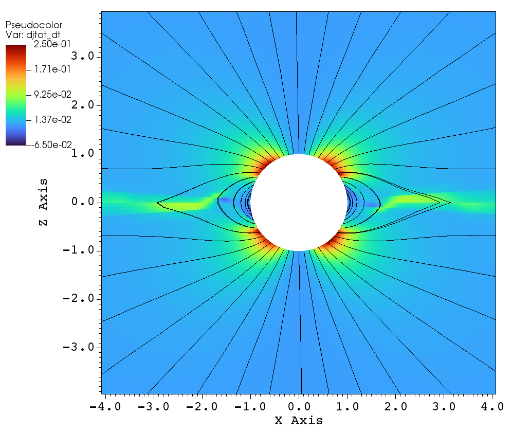
(a)

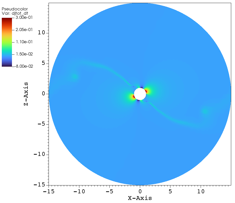
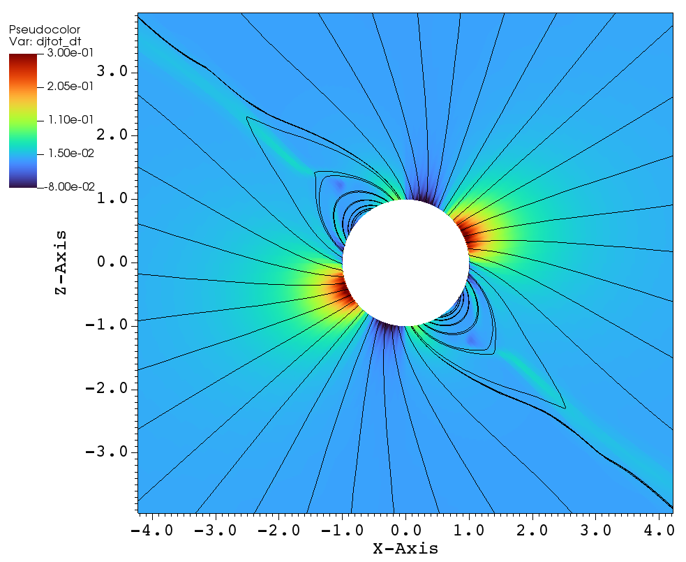
(b)

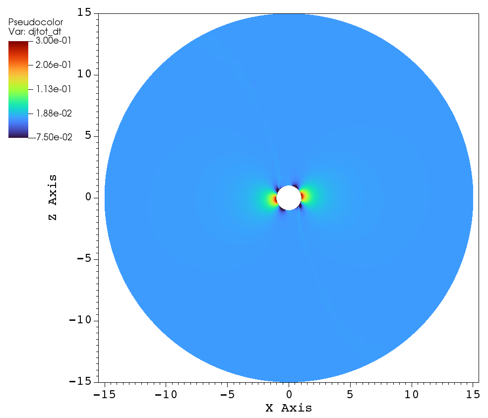
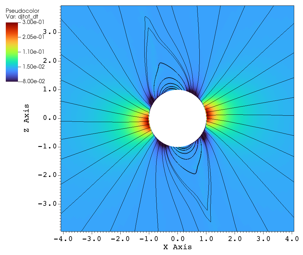
(c)

Figure 13: Cross section of total angular momentum flux $dj_{\rm tot}/dt$ ($\rm g\hskip 1.42262pts^{-2})$ in the $xz$-plane for $\eta_{\star}=10$, $W=0.5$: (a) no magnetic tilt ($\zeta=0\arcdeg$), (b) tilt $\zeta=45\arcdeg$, (c) tilt $\zeta=75\arcdeg$. The panels on the left show the large scale angular momentum flux in the entire xz-plane ($\pm 15R_{\star}$). The panels on the right show the zoomed in angular momentum flux in the inner xz-plane ($\pm 4R_{\star}$), with magnetic field lines overlaid.

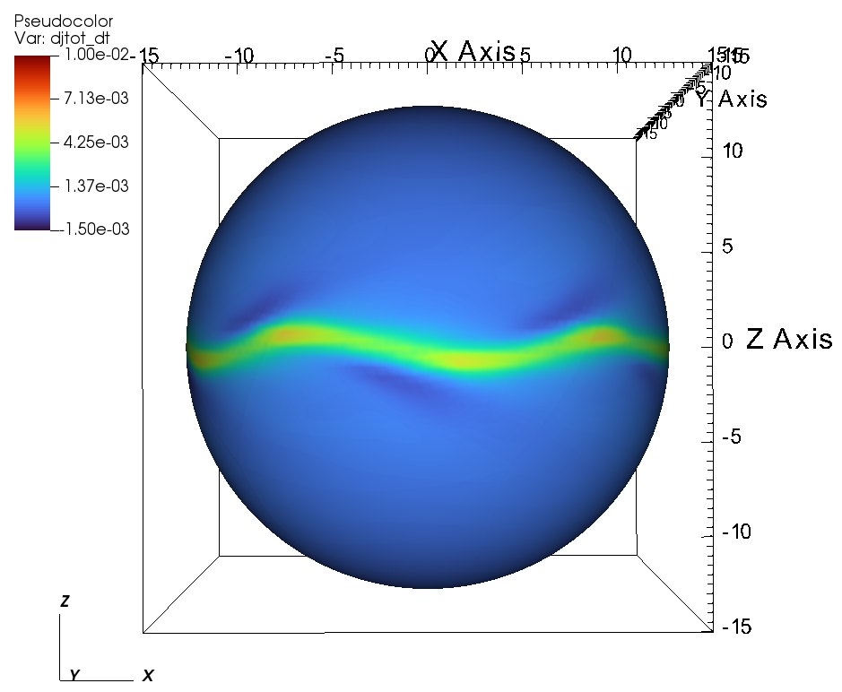
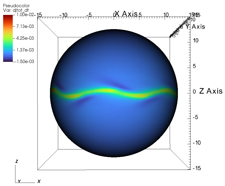
(a)                                                                         (b)

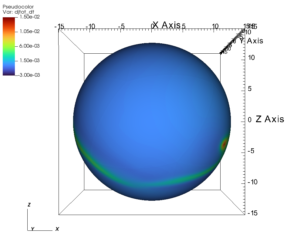
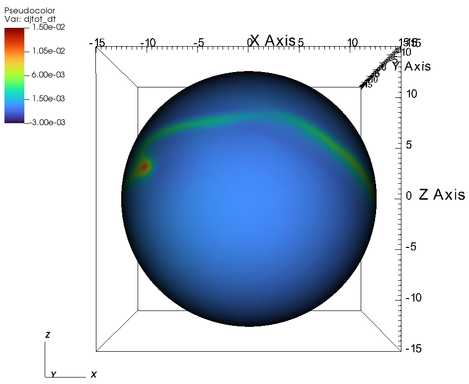
(c)                                                                         (d)

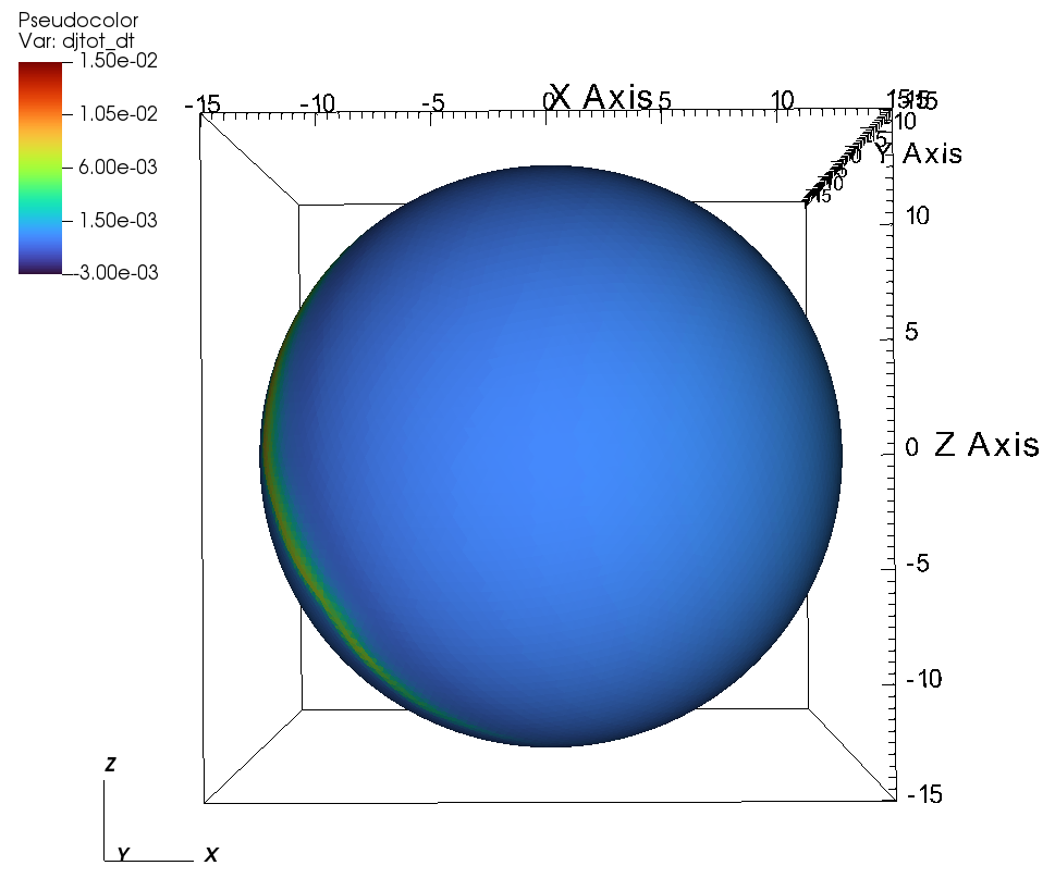
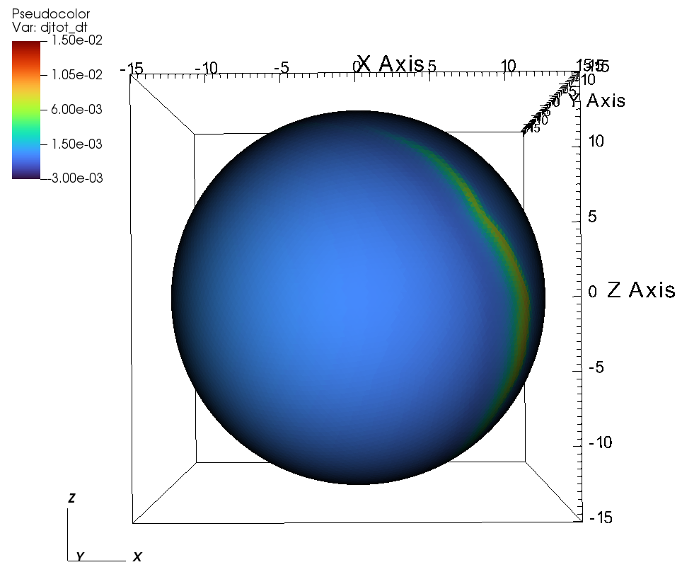
(e)                                                                         (f)

Figure 14: Total angular momentum flux $dj_{\rm tot}/dt$ ($\rm g\hskip 1.42262pts^{-2})$ at the outer surface for the case of $\eta_{\star}=10$ and $W=0.5$ showing: the front (a) and back (b) view for $\zeta=0\arcdeg$, the front (c) and back (d) view for $\zeta=45\arcdeg$, and the front (e) and back (f) view for $\zeta=75\arcdeg$.

With this preamble, the remainder of this section describes the angular momentum flux and angular momentum loss rate for the simulations listed in Table 1. Figure 13 displays the total angular momentum flux $dj_{\rm tot}/dt$ in the $xz-$plane for three tilt angles: (a) aligned rotation $\zeta=0\arcdeg$, (b) $\zeta=45\arcdeg$, and (c) $\zeta=75\arcdeg$. Figure 13a illustrates the total angular momentum flux for the case of aligned rotation. Far from the star, the angular momentum loss is expected to be maximal in the $xy-$plane (i.e. perpendicular to the axis of rotation) and minimal along the axis of rotation (i.e. the $z-$axis). This effect is shown in Figure 13a (i.e. in the left panel), where the large scale flow shows that $dj_{\rm tot}/dt$ is small along the rotation axis and substantially larger in the plane perpendicular to the rotation axis. However, in the in the zoomed right panel of Figure 13, we see that the angular momentum loss perpendicular to the plane of rotation is not maximal because closed magnetic loops near the stellar surface inhibit mass loss. Focusing on the right panel of Figure 13a, we see that the maximal angular momentum flux comes from the footpoints of the open magnetic field lines that connect to the equatorial outflow. Once the wind propagates past $R_{\rm A}$ the angular momentum flux is channeled towards the xy-plane.

Thus the angular momentum flux close to the surface of the star is maximal along the open field lines (${\bf B}_{\rm open}$) in the plane of rotation; i.e., where $|{\bf B}_{\rm open}\times{\bf\Omega}|$ is maximal. This result is especially evident for the case of of tilted-rotation with $\zeta=45\arcdeg$, shown in Figure 13b. In the zoomed panel, we see that the angular momentum loss close to the star is low along the magnetic equator, i.e. along the closed field lines, similar to the case of aligned rotation. Comparing the zoomed versions of Figs. 13a and 13b, in the $\zeta=45\arcdeg$ case the open field lines are present on either side of the magnetic equator. As a result of the magnetic tilt, the open field lines along the rotational equator, leading to have larger angular momentum flux close to the star. Conversely, the open field lines along the rotational $z-$axis have smaller angular momentum flux.

Similar observations can also be made for the $\zeta=75\arcdeg$ case (see Figure 13c), where the magnetic poles are nearly perpendicular to the axis of rotation. Hence, the total angular momentum loss close to the stellar surface is maximum near the magnetic poles, where the open field lines and the plane of rotation coincide.

Beyond the Alfvén radius, much of the angular momentum flux emerges along the magnetic equator because the angular momentum flux is channeled by the field lines. (see Figure 14). Figures 14a and 14b, show the total angular momentum flux at the outer boundary of the simulation, i.e. at a radius of $R\approx 15R_{\star}$. Figures 14a and 14b correspond to the case of aligned rotation. We see that most of the angular momentum flux is channeled by the magnetic field lines. Figures 14c-f, show the total angular momentum flux at the outer boundary of the simulation $R\approx 15R_{\star}$, for the case of tilted-rotation with $\zeta=45\arcdeg,75\arcdeg$. Here, similar to the aligned rotation, the angular momentum flux is influenced by the magnetic channeling of the wind and rotation. As we move farther from the star, the effect of rotation overpowers the strength of the magnetic field and the same can be observed from Figure 13b.

6.1 Radial variation of angular momentum loss

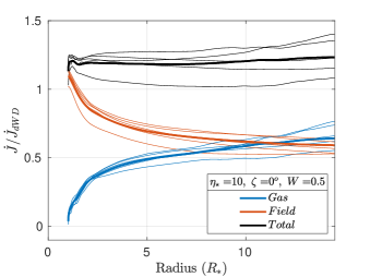
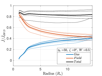
(a)                                                                   (b)

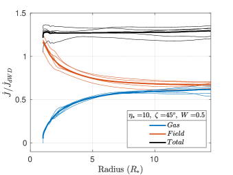
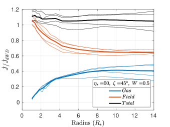
(c)                                                                   (d)

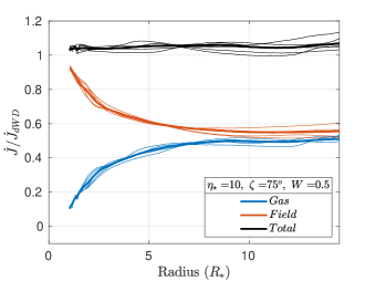
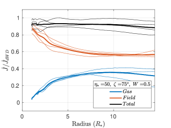
(e)                                                                   (f)

Figure 15: Angular momentum loss rate $\dot{J}$ as a function of stellar radius with rapid rotation ($W=0.5$) for gas in blue, magnetic field in red, and their total in black. $\dot{J}$ is normalized to the dipole Weber-Davis value for an aligned magnetic rotator $\dot{J}_{\rm dWD}$. Several quasi-steady state snapshots are shown with thin lines, and their time averages are indicated with thicker lines for the following cases: (a) $\eta_{\star}=10$ and $\zeta=0\arcdeg$, (b) $\eta_{\star}=50$ and $\zeta=0\arcdeg$, (c) $\eta_{\star}=10$ and $\zeta=45\arcdeg$, (d) $\eta_{\star}=50$ and $\zeta=45\arcdeg$, (e) $\eta_{\star}=10$ and $\zeta=75\arcdeg$, and (f) $\eta_{\star}=50$ and $\zeta=75\arcdeg$.

The strength of the dipole magnetic field is maximum at the photosphere, falling steeply ($1/r^{3}$) as we move away from the star. Due to this steep fall off, the angular momentum loss rate is predominantly magnetic close to the star. As we move away from the star, the magnetic component of the angular momentum loss rate ${\dot{J}_{\rm mag}}$ decreases and the gaseous component ${\dot{J}_{\rm gas}}$ increases, while keeping the total angular momentum loss rate ${\dot{J}_{\rm tot}}$ nearly constant. The total, magnetic and gas-borne angular momentum loss rates are plotted versus radius in Figure 15 as solid black, red and blue curves, respectively, for six different parameter sets. The $\dot{J}$ values in Figure 15, and the corresponding sixth column in Table 2, are normalized to the predicted $\dot{J}_{\rm dWD}$ in the dipole-modified Weber-Davis model (ud-Doula et al., 2009). The thin lines represent individual time snapshots, and the bold black, red and blue lines represent the average of the thin lines. As we expect from angular momentum conservation, the black (${\dot{J}_{\rm tot}}$) curves are essentially flat. However, we also see $\approx 10\%$ snapshot-to-snapshot variations, indicating that angular momentum loss is time variable.

These results are in line with the dynamics of magnetically channeled winds. 2D simulations carried out for the case of aligned rotation also show significant time variability in the angular momentum loss (ud-Doula et al., 2008). In Figure 15 for each $\eta_{\star}$ when the tilt angle $\zeta=0$, the gas is flung out with maximal centrifugal force. Comparing Figure 15a with 15c and also comparing Figure 15b with 15d, suggests that increasing the tilt angle $\zeta$ reduces the moment arm, thereby reducing the gas-borne angular momentum loss.

Further examination of the left ($\eta_{\star}=10$) and right ($\eta_{\star}=50$) panels in Figure 15 suggests that the angular momentum loss due to the field $\dot{J}_{\rm mag}$ increases with increasing $\zeta$, relative to the angular momentum loss due to the gas $\dot{J}_{\rm gas}$. This is especially evident in the higher-field panels on the left of Figure 15. At low $\zeta$, the gas in the magnetic equator experiences higher centrifugal force, and therefore contributes more to the total angular momentum loss. At high $\zeta$, the open field lines above the magnetic poles experience the highest centrifugal force, and therefore account for most of the total angular momentum loss.

6.2 Characteristic mass-loss and spindown time

Table 2: Mass loss rate, characteristic mass-loss time, angular momentum loss rate and spin-down time.

$\eta_{\star}$	$\zeta$	$W$	${\dot{M}}$	$\tau_{\rm mass}$	$\frac{{\dot{J}}_{\rm tot}}{{\dot{J}}_{\rm dWD}}$	$\frac{{\dot{J}}_{\rm tot}}{{\dot{J}}_{\rm dWD,B=0}}$	$\tau_{\rm spin}$
			($M_{\odot}~{}{\rm yr}^{-1}$)	(Myr)			(Myr)
0	$0\arcdeg$	0	1.49 $\times 10^{-6}$	16.7	…	…	…
0	$0\arcdeg$	0.5	1.70 $\times 10^{-6}$	14.7	1.04	1.04	2.50
10	$0\arcdeg$	0	6.92 $\times 10^{-7}$	36.1	…	…	…
10	$0\arcdeg$	0.5	8.37 $\times 10^{-7}$	29.8	1.29	5.81	0.44
10	$45\arcdeg$	0.5	7.96 $\times 10^{-7}$	31.4	1.35	6.07	0.42
10	$75\arcdeg$	0.5	5.88 $\times 10^{-7}$	42.5	1.05	4.73	0.55
50	$0\arcdeg$	0	4.35 $\times 10^{-7}$	57.4	…	…	…
50	$0\arcdeg$	0.5	4.58 $\times 10^{-7}$	54.6	0.95	7.73	0.34
50	$45\arcdeg$	0.5	5.84 $\times 10^{-7}$	42.8	1.24	10.12	0.26
50	$75\arcdeg$	0.5	4.41 $\times 10^{-7}$	56.7	0.96	7.81	0.33

The characteristic mass-loss time $\tau_{\rm mass}$ and the spin-down time $\tau_{\rm spin}$ can be approximated from the total mass loss rate ${\dot{M}}$ and the total angular momentum loss rate ${\dot{J}_{\rm tot}}$.

$$\tau_{\rm mass}=\dfrac{M_{\star}}{\dot{M}},$$ (17)

$$\tau_{\rm spin}=\dfrac{J}{\dot{J}_{\rm tot}}=\dfrac{kM_{\star}R_{\star}^{2}\Omega}{\dot{J}_{\rm tot}},$$ (18)

where $kM_{\star}R_{\star}^{2}$ is the star’s moment of inertia and $k\approx 0.1$ (ud-Doula et al., 2009). The characteristic mass-loss time and the spin-down time are presented in Table 2, along with the total angular momentum loss rate and the mass loss rate for the different sets of simulations carried out in this work. The total angular momentum loss rate presented in the sixth column of Table 2 is normalized to ${\dot{J}}_{\rm dWD}$, the predicted angular momentum loss rate from the dipole-modified Weber-Davis model. In column 7 we normalize ${\dot{J}_{\rm tot}}$ by ${\dot{J}}_{\rm dWD,B=0}$ the prediction of the non-magnetic Weber-Davis model. This last column highlights the expected increase in total angular momentum loss with increasing $\eta_{\star}$.

Comparing the non-magnetic cases, with and without rotation, the rotating case can be seen to have an increased mass-loss rate and a reduced characteristic mass-loss time. With the introduction of a magnetic field, we see a significant increase in the mass-loss time due to the higher magnetic confinement and the reduced mass-loss rate. In case of non-magnetic rotation, there is no spin-down due to magnetic braking and hence it has the longest spin-down time. This is because the angular momentum loss is carried by the gas. By the same token, the spin-down time is notably reduced as we go from $\eta_{\star}=10$ to $\eta_{\star}=50$, because of the increase in magnetic braking torque.

7 Summary and Conclusions

The presence of a dipolar magnetic field and its tilt with respect to the rotation axis can have notable influence on the mass outflow and the angular momentum outflow. The mass outflows from the O and B-type stars are very significant and thus influence the overall evolution of the star. Hence, it is inevitable that the presence of magnetic field and its orientation would play a significant role in the evolution of the O and B-type stars. The detailed simulation and analysis of the magnetic O and B-stars are discussed in the literature for the case of aligned rotation ud-Doula & Owocki (2002b); ud-Doula et al. (2008, 2009) with the help of 2D simulations.

For the simulation of spherical systems in full 3D, we have recently developed the Riemann Geomesh MHD code. The code is based on the spherical icosahedron-based meshing of the sphere. The surface of the sphere is mapped as uniformly as possible, which is a significant advance compared to an $r,\theta,\phi$ mesh. This eliminates the increased discretization errors stemming from singularities at the poles and the need for shorter time steps due to the concentration of mesh points at the poles.

In this work, we have carried out the 3D simulations of the magnetically channeled line driven winds for a template O star. For the first time, the simulations are done for a higher rotation rate ($0.5~{}\Omega_{crit}$) and larger magnetic field tilt angles ($0\arcdeg,45\arcdeg,75\arcdeg$); by utilizing the uniform meshing and state-of-the-art MHD algorithms of the Riemann Geomesh code. The simulations reach a quasi-steady state, as expected, and the mass-loss rate is observed to increase with rotation and decrease with increased magnetic field strength, due to the magnetic confinement of the wind. For the magnetized simulations, the wind exhibits the dynamics of magnetic channeling, as observed in previous 2D simulations. In addition, the results for the $45\arcdeg$ case demonstrates the interplay between the centrifugal force, which is maximum along the rotational equator, and the magnetic channeling, which is prominent along the magnetic equator.

Using these insights, we proceed to catalogue the mass-loss rate and angular momentum loss rate for different magnetic-field strengths, tilt angles and rotation rates. The spatial variations in total angular momentum flux ($dj_{\rm tot}/dt$) are examined for different magnetic tilt angles, with the help of images at the cross-section plane, as well as, at the outer surface of the simulation domain. Near the stellar surface, the maximal total angular momentum flux ($dj_{\rm tot}/dt$) is observed where the open magnetic field lines align with the plane of rotation. Farther from the star, the maximal angular momentum flux ($dj_{\rm tot}/dt$) is aligned with the confinement of magnetic field lines, emanating from either sides of the magnetic equator.

The gaseous, magnetic and total angular momentum loss rates ${\dot{J}}$ are computed as a function of radius, and plotted for different tilt angles and magnetic field strengths. With the corresponding mass-loss rates, the characteristic mass-loss time and spin-down time are tabulated for the simulations carried out in this work. The results show a longer mass-loss time with increasing magnetic field strength, which tracks the reduced mass-loss rate. We also find faster spin-down time with increasing magnetic field strength, showing the role of magnetic braking torque on the rotation of the star.

These simulations are the very first that have been reported with a code that can handle all possible tilt angles of the magnetic dipole with respect to the rotation axis. The use of a mapped mesh makes these simulations somewhat more expensive, but this comes with the tremendous advantage of full geometric generality. While we are not restricted to dipolar fields, we have focused on dipolar fields in this study. In order to develop a comprehensive understanding of the relations between, $\eta_{\star},~{}\zeta,~{}W$ and ${\dot{M}},{\dot{J}}$, a much larger set of data with more finer variations in $\eta_{\star},~{}\zeta,~{}W$ is necessary. Therefore, this is planned for the next set of study and it will be elaborated in a subsequent paper.

Data Availability

The data underlying this article are available in the article and in its online supplementary material.

Appendix A Description of the MHD Equations

The governing MHD equations of this simulation study are presented below. The magnetic field ${\bf B}$ is split into a curl-free background field ${\bf B_{0}}$ and a time evolving field ${\bf B_{1}}$. The total magnetic field is defined to be, ${\bf B}={\bf B_{0}}+{\bf B_{1}}$. Upon imposing the vector identities, the governing equations take the following forms (Powell, 1994; Guo et al., 2016),
i) conservation of mass

$$\frac{\partial\rho}{\partial t}+\nabla\cdot\left(\rho{\bf v}\right)=0$$ (A1)

where, $\rho$ is the density and ${\bf v}$ is the velocity of the fluid
ii) conservation of momentum

$$\frac{\partial(\rho{\bf v})}{\partial t}+\nabla\cdot\left[\rho{\bf v}{\bf v}+P{\bf I}+\frac{1}{8\pi}{B_{1}}^{2}{\bf I}+\frac{1}{4\pi}\left(({\bf B_{0}}\cdot{\bf B_{1}}){\bf I}-{\bf B_{1}}{\bf B}-{\bf B_{0}}{\bf B_{1}}\right)\right]=\rho~{}{\bf g_{\rm tot}}$$ (A2)

where, $P$ is the pressure and ${\bf g}_{\rm tot}$ is the total net acceleration coming from the external forces. For this simulation, it comprises of CAK line acceleration, gravitational acceleration and the centrifugal and Coriolis accelerations arising due to rotation. This can be expressed as,

$${\bf g}_{\rm tot}=g_{CAK}{\bf{\hat{r}}}+g_{\rm grav}{\bf{\hat{r}}}-2~{}{\bf\Omega}\times{\bf v}-{\bf\Omega}\times\left({\bf\Omega}\times{\bf r}\right)$$

where, ${\bf\Omega}$ is the angular velocity vector and ${\bf{\hat{r}}}$ is the unit vector along the radial direction.
iii) conservation of energy

$$\frac{\partial E}{\partial t}+\nabla\left[\left(E+P+\dfrac{{B_{1}}^{2}}{8\pi}+\dfrac{{{\bf B_{0}}\cdot{\bf B_{1}}}}{4\pi}\right){\bf v}-\dfrac{({\bf v}\cdot{\bf B_{1}}){\bf B}}{4\pi}\right]=\rho{\bf v}\cdot{\bf g}_{tot}$$ (A3)

where, $E$ is the energy density. These are isothermal simulations, therefore the energy equation is not used however, for the sake of completion this is included here. The pressure $P$ is then defined using the sound speed $v_{s}$ as $P=\rho v_{s}^{2}$.
iv) induction equation

$$\frac{\partial{\bf B_{1}}}{\partial t}-\nabla\times({\bf v}\times{\bf B})=0$$ (A4)

References

- Balsara (2017) Balsara, D. S. 2017, Living Reviews in Computational Astrophysics, 3, 2, doi: 10.1007/s41115-017-0002-8
- Balsara & Dumbser (2015) Balsara, D. S., & Dumbser, M. 2015, Journal of Computational Physics, 287, 269, doi: 10.1016/j.jcp.2014.11.004
- Balsara et al. (2019) Balsara, D. S., Florinski, V., Garain, S., Subramanian, S., & Gurski, K. F. 2019, MNRAS, 487, 1283, doi: 10.1093/mnras/stz1263
- Balsara et al. (2020) Balsara, D. S., Garain, S., Florinski, V., & Boscheri, W. 2020, Journal of Computational Physics, 404, 109062, doi: 10.1016/j.jcp.2019.109062
- Castor et al. (1975) Castor, J. I., Abbott, D. C., & Klein, R. I. 1975, ApJ, 195, 157, doi: 10.1086/153315
- Daley-Yates et al. (2019) Daley-Yates, S., Stevens, I. R., & ud-Doula, A. 2019, MNRAS, 489, 3251, doi: 10.1093/mnras/stz1982
- Florinski et al. (2020) Florinski, V., Balsara, D. S., Garain, S., & Gurski, K. F. 2020, Computational Astrophysics and Cosmology, 7, 1, doi: 10.1186/s40668-020-00033-7
- Friend & Abbott (1986) Friend, D. B., & Abbott, D. C. 1986, ApJ, 311, 701, doi: 10.1086/164809
- Gagné et al. (2005) Gagné, M., Oksala, M. E., Cohen, D. H., et al. 2005, ApJ, 628, 986, doi: 10.1086/430873
- Grunhut et al. (2017) Grunhut, J. H., Wade, G. A., Neiner, C., et al. 2017, MNRAS, 465, 2432, doi: 10.1093/mnras/stw2743
- Guo et al. (2016) Guo, X., Florinski, V., & Wang, C. 2016, Journal of Computational Physics, 327, 543, doi: 10.1016/j.jcp.2016.09.057
- Howarth & van Leeuwen (2019) Howarth, I. D., & van Leeuwen, F. 2019, MNRAS, 484, 5350, doi: 10.1093/mnras/stz291
- Langer (2012) Langer, N. 2012, ARA&A, 50, 107, doi: 10.1146/annurev-astro-081811-125534
- Maeder & Meynet (2000) Maeder, A., & Meynet, G. 2000, ARA&A, 38, 143, doi: 10.1146/annurev.astro.38.1.143
- Owocki (2004) Owocki, S. 2004, in EAS Publications Series, Vol. 13, EAS Publications Series, ed. M. Heydari-Malayeri, P. Stee, & J. P. Zahn, 163–250, doi: 10.1051/eas:2004055
- Owocki et al. (2020) Owocki, S. P., Shultz, M. E., ud-Doula, A., et al. 2020, MNRAS, 499, 5366, doi: 10.1093/mnras/staa2325
- Owocki & ud-Doula (2004) Owocki, S. P., & ud-Doula, A. 2004, ApJ, 600, 1004, doi: 10.1086/380123
- Petit et al. (2013) Petit, V., Owocki, S. P., Wade, G. A., et al. 2013, MNRAS, 429, 398, doi: 10.1093/mnras/sts344
- Powell (1994) Powell, K. 1994, An approximate Riemann solver for magnetohydrodynamics (that works in more than one dimension), CWI
- Ruen & Bulatov (2012) Ruen, T., & Bulatov, V. 2012, Zeroth stellation of icosahedron. https://commons.wikimedia.org/wiki/File:Zeroth_stellation_of_icosahedron.png
- Schöller et al. (2017) Schöller, M., Hubrig, S., Fossati, L., et al. 2017, A&A, 599, A66, doi: 10.1051/0004-6361/201628905
- Shultz et al. (2020) Shultz, M. E., Owocki, S., Rivinius, T., et al. 2020, MNRAS, 499, 5379, doi: 10.1093/mnras/staa3102
- ud-Doula & Nazé (2016) ud-Doula, A., & Nazé, Y. 2016, Advances in Space Research, 58, 680, doi: 10.1016/j.asr.2015.09.025
- ud-Doula et al. (2014) ud-Doula, A., Owocki, S., Townsend, R., Petit, V., & Cohen, D. 2014, MNRAS, 441, 3600, doi: 10.1093/mnras/stu769
- ud-Doula & Owocki (2002a) ud-Doula, A., & Owocki, S. P. 2002a, ApJ, 576, 413
- ud-Doula & Owocki (2002b) —. 2002b, ApJ, 576, 413, doi: 10.1086/341543
- ud-Doula et al. (2008) ud-Doula, A., Owocki, S. P., & Townsend, R. H. D. 2008, MNRAS, 385, 97, doi: 10.1111/j.1365-2966.2008.12840.x
- ud-Doula et al. (2009) —. 2009, MNRAS, 392, 1022, doi: 10.1111/j.1365-2966.2008.14134.x
- ud-Doula et al. (2013) ud-Doula, A., Sundqvist, J. O., Owocki, S. P., Petit, V., & Townsend, R. H. D. 2013, MNRAS, 428, 2723, doi: 10.1093/mnras/sts246
- ud-Doula et al. (2006) ud-Doula, A., Townsend, R. H. D., & Owocki, S. P. 2006, ApJ, 640, L191, doi: 10.1086/503382
- Wade et al. (2016) Wade, G. A., Neiner, C., Alecian, E., et al. 2016, MNRAS, 456, 2, doi: 10.1093/mnras/stv2568
- Weber & Davis (1967) Weber, E. J., & Davis, Leverett, J. 1967, ApJ, 148, 217, doi: 10.1086/149138