Precise and Generalized Robustness Certification for Neural Networks

Abstract

The objective of neural network (NN) robustness certification is to determine if a NN changes its predictions when mutations are made to its inputs. While most certification research studies pixel-level or a few geometrical-level and blurring operations over images, this paper proposes a novel framework, GCert, which certifies NN robustness under a precise and unified form of diverse semantic-level image mutations. We formulate a comprehensive set of semantic-level image mutations uniformly as certain directions in the latent space of generative models. We identify two key properties, independence and continuity, that convert the latent space into a precise and analysis-friendly input space representation for certification. GCert can be smoothly integrated with de facto complete, incomplete, or quantitative certification frameworks. With its precise input space representation, GCert  enables for the first time complete NN robustness certification with moderate cost under diverse semantic-level input mutations, such as weather-filter, style transfer, and perceptual changes (e.g., opening/closing eyes). We show that GCert enables certifying NN robustness under various common and security-sensitive scenarios like autonomous driving.

1 Introduction

While neural networks (NNs) have prosperous development, their robustness issue remains a serious concern. Specifically, a NN’s prediction can be easily changed by applying small mutations over its input (e.g., via adversarial attacks [26, 29, 50]). This has led to severe outcomes in security-critical applications like autonomous driving [8, 2].

As a principled solution to mitigate the robustness issue and adversarial attacks, NN robustness certification has been actively studied [22, 13, 11, 56, 39, 45, 9]. Given a mutation $\tau$ and a tolerance $\|\delta_{\max}\|$ (which decides the maximum extent to which the mutation is applied) over an input image, it aims to certify that the NN’s prediction for all mutated images remains within the tolerance. The primary challenge is to formulate the input space determined by $\tau$ and $\|\delta_{\max}\|$ in a precise and analysis-friendly manner. It is evident that the input space has an infinite number of mutated images, and in practice, various input space abstraction schemes are applied, e.g., using the interval and zonotope abstract domains originated from the abstract interpretation theory [15]. Technically, verifying NNs can be both sound and complete (NNs are generally loop-free) [66, 60, 20, 61, 32].

In practice, de facto NN certification delivers sound analysis, while most of them fail to provide complete analysis simultaneously. This is primarily due to the over-approximated (imprecise) input space formed over diverse real-world mutations. Most certification works focus on pixel-level input mutations (e.g., adding $\ell_{p}$-norm noise) whose resulting input space is linear and easy for analysis. Nevertheless, pixel-level mutations are simple and insufficient to subsume various mutations that may occur in reality. Note that recent testing and adversarial attacks toward NNs have been using geometrical mutations [65, 64] (e.g., rotation), blurring [65, 58], and more advanced mutations including weather filter [74, 68], style transfer [23, 69, 68], and perceptual-level (e.g., changing hairstyle) mutations [18, 67, 70].

It is challenging to take into account the aforementioned mutations, because the input spaces formed by applying those mutations over an image are non-linear, making a precise input space representation difficult. Moreover, some mutations even do not have explicit mathematical expressions. Recent research considers geometrical mutations, but over-approximates the input space [56, 11, 47]. As a result, it can only support incomplete certification, which may frequently fail due to the over-approximation (“false positives”) rather than non-robustness (“true positives”). Other works support blurring, by only offering (incomplete) probabilistic certification: a NN is certified as “robust” with a probability [42, 27, 21]. A probabilistic guarantee is less desirable in security-critical scenarios. Also, existing techniques are typically mutation-specific; supporting new mutations is often challenging and costly, and may require domain expertise.

Besides pixel-level mutations, adversarial NN attacks also adopt semantic-level mutations, which change image semantics holistically. Generative models (e.g., GAN [25], VAE [35]), which map points from a latent space to images, can generate infinite images with diverse semantics. By using the latent space of generative models and their image generation capability, we explore a principled technical solution of forming input space representations of various semantics-level mutations to support NN certification.

Conceptually, mutating an image $x$ via a generative model is achieved by moving its corresponding latent point $z$ in the latent space. However, given the latent spaces of common generative models, mutating $x$ would only generate mutated images $x^{\prime}$ with arbitrarily changed content. Thus, we re-formulate the latent spaces of generative models in a regulated form (see below), thereby offering a precise and analysis-friendly input space representation to support complete NN certification. We re-form the latent spaces with the aim of achieving two key objectives: 1) independence: image semantics corresponding to different mutations change independently, and 2) continuity: if certain semantics are mutated, they should change continuously. With independence, different semantic-level mutations are represented as orthogonal directions in the latent space, and mutating a semantics instance (e.g., hair style) is conducted by moving a point along the associated direction in the latent space without disturbing other semantics. Moreover, continuity ensures latent points of all mutated inputs are exclusively included in a segment in the latent space.

Our analysis for the first time incorporates a broad set of semantic-level mutations, including weather filter (e.g., rainy), style transfer, and perceptual mutations, to deliver comprehensive and practical NN certification. Our approach is agnostic to specific generative models and enables certification towards mutations that have no explicit math expression. It offers precise input space representations, and consequently enables the first complete certification for semantic-level mutations with largely reduced cost (from exponential to polynomial). Also, since mutated inputs are represented as a segment in the latent space (see Sec. 4), our approach can be integrated into recent quantitative certification frameworks [46], offering fine-grained bounds to depict NN robustness.

We implement our approach in a framework named GCert. We conduct both qualitative and quantitative evaluations to assess the diversity and correctness of semantic-level mutations enabled in GCert. Our precise input space representation is around $60\%$ tighter than SOTA results for geometrical mutations. Moreover, we show that GCert can be smoothly leveraged to boost de facto complete, incomplete, or quantitative certification frameworks toward various NNs under usage scenarios like classification, face recognition, and autonomous driving. We also cross-compare how different mutations can influence NN robustness. We then present both theoretical and empirical cost analysis for GCert, illustrating its applicability. Overall, we have the following contributions:

• This work enables the first sound and complete NN certification under various real-world semantic-level mutations, which is a major step toward practical NN robustness certification. We uniformly re-formulate a broad set of semantic-level image mutations as mutations along directions in the latent space of generative models. Moreover, this work for the first time certifies NN robustness under advanced mutations, such as weather-filter, style transfer, and perceptual mutations.

• We identify two key requirements, independence and continuity, that turn the latent space associated with common generative models into a precise and analysis-friendly form for NN certifications. We give formal analysis and practical solutions to achieve these requirements. Consequently, input spaces under semantic-level mutations can be represented precisely, for the first time enabling practical complete/quantitative certification.

• Evaluations illustrate the correctness and diversity of our delivered semantic-level mutations. Our approach manifests high practicality and extendability, as it can be applied on any common generative models and smoothly incorporated into existing certification frameworks. We certify different NNs under various security-sensitive scenarios and comprehensively study NN robustness w.r.t. the NN structure, training data, and input mutations.

Research Artifact. We release the code and data at https://github.com/Yuanyuan-Yuan/GCert [1].

2 Preliminary & Background

In this section, we first introduce NN robustness certification, and then discuss how various input mutations are performed. We then briefly review existing input representation solutions and their limitations to motivate this research.

2.1 NN Robustness Certification

Following existing works [22, 73, 13, 42, 48, 39, 20], we focus on robustness certification of image classification, a common and essential NN task. Certifying other NN tasks, objectives (e.g., fairness), and types of inputs (e.g., audio, text) can be easily extended from GCert; see Sec. 8.

Problem Statement. As illustrated in Fig. 1, NN robustness certification comprises the following components: 1) a certification framework $\phi$, 2) a target NN $f$, 3) an input image $x$, 4) a mutation scheme $\langle\tau,\delta\rangle$, where $\tau$ is a function specifying the mutation over $x$ and $\delta$ decides to what extent the mutation is performed (e.g., $\delta$ denotes the rotating angle if $\tau$ is rotation), and 5) tolerance $\|\delta_{\max}\|$, specifying the maximal value (often in the form of norm since $\delta$ can be a vector) of $\delta$.

Threat Model. Our threat model is aligned with existing works in this field [22, 73, 13, 42, 48, 39, 20]. That is, we aim to certify that when one mutation scheme $\langle\tau,\delta\rangle$, which is bounded by $\|\delta_{\max}\|$ (i.e., $0\leq\|\delta\|\leq\|\delta_{\max}\|$), is applied on an image $x$, whether the NN $f$ has the same prediction with $x$ over all mutated images. As will be detailed in Fig. 1, the mutations can be introduced by variations in real-world unseen inputs or attackers who are generating adversarial examples (AEs) [24] using different methods. A certified NN is robust to those unseen or adversarial inputs, and we do not assume any particular AE generation method. Formally, we study if the following condition holds.

$$f(x)=f(x^{\prime}),\;\forall x^{\prime}\in\{\tau(x,\delta)\;|\;0\leq\|\delta\|\leq\|\delta_{\max}\|\}$$ (1)

For instance, if $\tau$ is rotation and $\|\delta_{\max}\|$ is set to $30^{\circ}$, the certification aims to certify whether $f$ changes its prediction for $x$ if $x$ is rotated within $30^{\circ}$. A certification is successful if it certifies that Eq. 1 always holds; it fails otherwise. We now introduce input mutation and the certification procedure.

Abstracting Mutated Inputs. Typical challenges include 1) considering representative real-world image mutations, and 2) forming an input space representation $I$ which should be as close to all $x^{\prime}=\tau(x,\delta)$ as possible [11, 42, 21, 27, 49]. Image mutations $\tau$ are typically implemented in distinct and often challenging ways (see Sec. 2.2), and therefore, previous works are usually specific to one or a few mutations that are easier to implement and less costly. Even worse, the input space formed by $\tau(x,\delta)$ often captures unbounded sets of images, and one cannot simply enumerate all images $\tau(x,\delta)$ and check Eq. 1. In practice, various abstractions are performed over $\tau(x,\delta)$ to offer an analysis-friendly representation $I$ (which are generally imprecise; see below). For instance, the interval $[a,b]$ can be viewed as an abstraction of a pixel value $v$ mutated within a bound $a\leq v\leq b$. Nevertheless, $\tau(x,\delta)$ resulted from most mutation schemes are non-linear, making a proper $I$ (without losing much precision) fundamentally challenging.

Certification Procedure. Given input space representation $I$, certification propagates it through NN layers to obtain outputs, which are then checked against Eq. 1. Due to Rice’s theorem, constructing a sound and complete certification (verification) over non-trivial program properties is undecidable [53], and most verification tools are unsound [44]. Nevertheless, for NNs (which are generally loop-free), it is feasible to deliver both sound and complete certification (e.g., with solver-based approaches) [60, 61, 20]; the main challenge is scalability with the size of NNs (e.g., #layers). In fact, de facto certification tools consistently offer sound analysis, such that when the NN $f$ violates a property under an input $x^{\prime}\in I$, the certification can always reveal that (i.e., no false negative).

On the other hand, the “completeness” may not be guaranteed: the certification is deemed complete if it proves Eq. 1 holds when it actually holds (i.e., no false positive). Nevertheless, complete certifications [20, 61, 73, 60, 66] are often challenging to conduct. A complete certification procedure requires the input space representation $I$ must be precise; i.e., $I$ should exclusively include all mutated inputs $x^{\prime}\in\tau(x,\delta)$. To date, complete certifications are limited to a few pixel-level mutations [60, 20, 61, 41] and the overall cost is exponential to the neuron width (the maximum #neurons in a layer).

Incomplete certifications [48, 56, 22] gradually over-approximate the input representation along the propagation to reduce the modeling complexity. An incomplete certification, however, cannot guarantee that it can prove Eq. 1 which actually holds. Hence, we may often encounter false positives, treating a safe NN as “unknown/unsafe.”

Figure 1: Certification procedures and the position of GCert.

Design Focus & Position w.r.t. Previous Works

A diverse set of real-world image mutation schemes (see Sec. 2.2) are used in attacking NNs. These mutations are holistically categorized as simple $M_{s}$, complex $M_{c}$, and advanced $M_{a}$. As shown in Fig. 1, most prior works employ $M_{s}$ (e.g., adding noise bounded by $\ell_{p}$-norm) whose input space is linear and putting primary efforts into optimizing the certification frameworks. Existing complete certifications are limited to simple mutations. $M_{c}$’s input space is non-linear and over-approximated, and therefore, certifications based on $M_{c}$ are only incomplete. $M_{a}$ was infeasible, since they do not have “explicit” math expressions. It is thus unclear how to represent their resulting input space.

The design focus of GCert is orthogonal to previous works: it addresses a fundamental and demanding challenge, i.e., how to offer a precise and unified input space representation $I$ over a wide range of real-world semantic-level mutations $\tau$ (i.e., those belonging to $M_{c}$ and $M_{a}$). The abstracted $I$ can be integrated with de facto certification frameworks, and consequently enables sound, complete, and even quantitative (which quantifies the percentage of mutated inputs that retain the prediction) NN certification with moderate cost.

2.2 Real-World Diverse Image Mutations

Fig. 2 hierarchically categorizes image mutations that have been adopted in testing and attacking NNs by prior works. We introduce each category below.

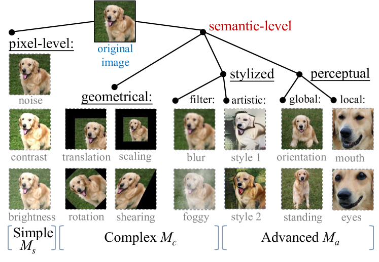
Figure 2: Hierarchical categorization of image mutations. Geometrical, stylized, and perceptual mutations belong to semantic-level because they holistically change semantics of the original image. GCert enables all semantic-level mutations ($M_{c}$ and $M_{a}$) and offers an analysis-friendly, linear, and unified representation for complete certification.

Simple $M_{s}$. Mutations of this category directly operate on image pixels. Given an input image $x$, one $M_{s}$ can be expressed as either $x+\delta$, or $x\times\delta$. For example, to change image brightness (or contrast), a real number is added to (or multiplied with) all pixel values. Similarly, to add noise, a vector $\delta$ of random values is added on $x$. Overall, pixel values of mutated images change linearly with the norm of $\delta$. Therefore, an input space $I$ corresponding to these mutations can be precisely formed and propagated along NN layers.

Complex $M_{c}$ — Geometrical. These mutations (a.k.a. affine mutations) change geometrical properties (e.g., position, size) but preserve lines and parallelism (i.e., move points to points) of input images. For any pixel in the $(i,j)$-th location (which is a relative location to the centering point) of an image $x$, geometrical mutations first compute $[i^{\prime},j^{\prime}]^{\intercal}=\bm{A}\times[i,j]^{\intercal}+\bm{b}$, where $\bm{A}$ is a $2\times 2$ matrix and $\bm{b}$ is a 2-dimensional vector. Different $\bm{A}$ and $\bm{b}$ specify different geometrical schemes. For instance, if $\tau$ is rotation, then

$$\scriptsize\begin{bmatrix}i^{\prime}\\ j^{\prime}\\ \end{bmatrix}=\begin{bmatrix}\cos\delta&-\sin\delta\\ \sin\delta&\cos\delta\\ \end{bmatrix}\times\begin{bmatrix}i\\ j\\ \end{bmatrix}+\begin{bmatrix}0\\ 0\\ \end{bmatrix}=\begin{bmatrix}i\cos\delta-j\sin\delta\\ i\sin\delta+j\cos\delta\\ \end{bmatrix},$$

where $\delta$ is the rotating angle ($\delta>0$ for left rotation). Each pixel in the mutated image $x^{\prime}$ is decided as $x^{\prime}_{i^{\prime},j^{\prime}}=x_{i,j}$. Since $i^{\prime}$ and $j^{\prime}$ should be integers, interpolation is further applied on pixels around $i^{\prime}$ and $j^{\prime}$ if they are non-integer [11, 5, 42]. Fig. 3(a) reports the pixel values of a four-pixel image when it is right rotated $90^{\circ}$ three times. Fig. 3(b) visualizes the first two pixels across three mutations. The correlation between pixel values and $\delta$ is apparently non-linear in geometrical mutations, which impedes presenting a precise input space $I$ for geometrical mutations.

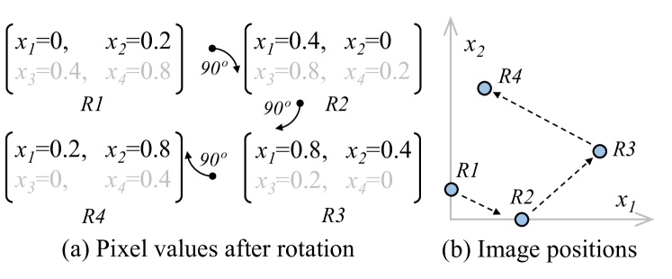
Figure 3: Positions of rotated images. In (a), a four-pixel image $R1$ is right rotated $90^{\circ}$ three times into $R2$, $R3$, and $R4$. Their positions, when only considering the first two pixels, are shown in (b). Dashed arrows only point the direction where rotating angle is increased; intermediate images between two marked images are omitted in (b).

Complex/Advanced $M_{c}$/$M_{a}$ — Stylized. As in Fig. 2, both filter-based and artistic mutations change an image’s “visual style.” Filter-based mutations first define a domain-specific filter (such as blurring, rainy, or foggy), and then apply the filter to an image to simulate varying real-world scenarios. For example, as often in auto-driving testing [58, 74], a driving scene image is applied by a foggy filter to stress the NN for making correct driving decision. Artistic mutations perform more extensive mutations to largely change the color scheme of an image. Recent studies show that artistic-stylized images reveal the texture-bias of NNs and effectively flip their predictions [23, 30]. Nevertheless, artistic stylizing is never explored in NN robustness certification.

Advanced $M_{a}$ — Perceptual. Perceptual mutations aim to change perceptual properties of input images, e.g., making a lying dog stand up (as shown in Fig. 2). Holistically, its effectiveness relies on the manifold hypothesis [12, 76], which states that perceptually meaningful images lie in a low-dimensional manifold that encodes their perceptions (e.g., facial expressions, postures). In practice, generative models are widely used for approximating manifold, such that they can generate infinite and diverse mutated images after being trained on a finite number of images. Intuitively, for dog images, since real-world images subsume various perceptions, generative models can infer a posture mutation, “standing $\rightarrow$ lying”, based on existing standing and lying dogs. The trained generative model then applies the mutation on other (unseen) images. Although perceptual mutations facilitate assessing NNs for more advanced properties, they are hard to control (e.g., several perceptions may be mutated together). Moreover, perceptual mutations result in non-smooth mutations, e.g., the mutated image is largely altered with a small perturbation on $\delta$. These hurdles make them less studied in NN certification.

2.3 Input Space Representation $I$

As noted in Sec. 2.1 and Fig. 2, existing NN certifications only support $M_{s}$ and $M_{c}$ mutations. Below, we review existing input representations $I$ and discuss their limitations.

Precise $I$ for $M_{s}$. Early works primarily consider pixel-wise mutations, due to their simpler math forms and the derived linear input space. $M_{s}$ primarily focuses on adding noise, and $\|\delta\|$, accordingly, is computed using the $\ell_{p}$-norm:

$$\scriptsize\|\delta\|_{p}=(\delta[0]^{p}+\delta[1]^{p}+\dots+\delta[m-1]^{p})^{\frac{1}{p}},\;\delta\in\mathbb{R}^{m}.$$

As noted in Sec. 2.2, input space $I$ derived from $M_{s}$ can be precisely represented, i.e., $I$ exclusively includes all mutated inputs. Current complete certifications only support $M_{s}$.

Imprecise $I$ for $M_{c}$. An explicit and rigorous math form may be required to form input space $I$ over each $M_{c}$ scheme. Hence, prior certification works only consider a few geometrical/filter-based mutations. These works are classified as deterministic and probabilistic, depending on if the certification proves that Eq. 1 is always or probabilistically holds.

Deterministic. DeepPoly [56] depicts the input space of geometrical transformations as intervals, which is imprecise and frequently results in certification failure [11]. Though it can be optimized by Polyhedra relaxation, Polyhedra relaxation may hardly scale to geometric transformations [11], because its cost grows exponentially with the number of variables. Also, the represented input space with Polyhedra relaxation is still imprecise. DeepG [11] computes linear constraints for pixel values under a particular geometrical mutation. It divides possible $\delta$ values into splits before sampling from these small splits to obtain unsound constraints (which miss some mutated images) for pixel values. Later, based on the maximum change in pixel values, it turns unsound constraints into sound ones by including all mutated images but also extra ones. GCert, however, can precisely represent the input space $I$ with a polynomial cost.

GenProve [46] uses generative models to enhance certification. However, the generative model is used for generating interpolations between the original image and the mutated image. Several problems arise: 1) for advanced, perceptual mutations (not considered in GenProve), the target image for interpolation may not always be accessible, e.g., for a dog, we must have two images where it is standing in one and lying in another; 2) interpolations are not guaranteed to only follow the semantic differences between the original image and the mutated image, e.g., interpolated images between faces of different orientations may have gender changed as well; and 3) interpolations are not always “intermediate images” between the original and mutated ones, e.g., when interpolating between an image and its $30^{\circ}$-rotated mutant using generative model, a $90^{\circ}$-rotated image may exist in the interpolations.

Probabilistic. Other works apply randomized smoothing on the target NN to support more mutations (e.g., filter-based mutations) and improve scalability [42, 21, 27]. In general, different smoothing strategies are tailored to accommodate mutations of different mathematical properties (e.g., translation, rotation [42]). However, due to smoothing, Eq. 1 can only be probabilistically certified, if the certification succeeds. Therefore, they are less desirable in security-critical tasks (e.g., autonomous driving), since there remains a non-trivial possibility that a “certified” NN violates Eq. 1, thus leading to severe outcomes and fatal errors. GCert focuses on deterministic certification under semantic-level mutations, although it is technically feasible to bridge GCert with probabilistic certification frameworks as well.

3 Generative Models and Image Mutations

Generative models like GAN [25], VAE [35], and GLOW [36] are popular for data generation. As introduced in Sec. 2.2, they are widely used for approximating manifold, which encodes semantics of real-world images. In brief, a generative model maps a collection of real-world images as points in a low-dimensional latent space that follows a continuous distribution (e.g., normal distribution) [12, 25]. This way, “intermediate images” between two known images can be inferred. Therefore, by randomly sampling points from the latent space, infinite diverse, high-quality images can be generated.

Let the latent space of generative model $G$ be $\mathcal{Z}$, generating an image $x$ can be expressed as $G:z\in\mathcal{Z}\rightarrow x\in\mathcal{M}$, where $\mathcal{M}$ denotes the manifold of images. Note that $\mathcal{M}$, approximated by $G(\mathcal{Z})$, does not equal the pixel space of images, because most “images” with random pixel values are meaningless. Conceptually, $\mathcal{M}$ is much smaller than the pixel space.

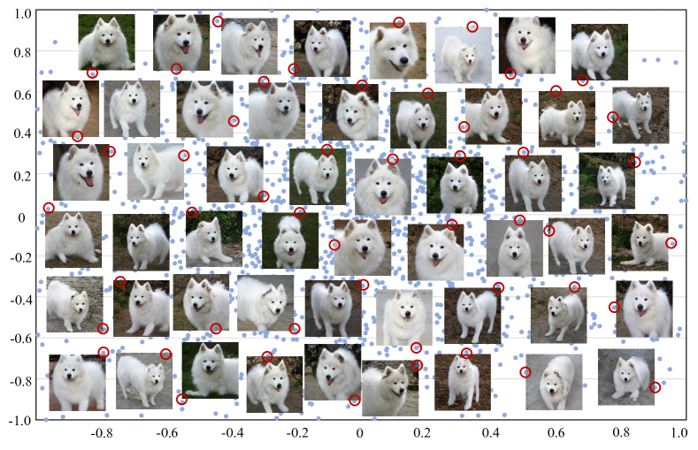
Figure 4: Moving $z$ in the latent space of BigGAN [14] and the derived images which have diverse semantics. Since the generative model is not regulated, these semantics change arbitrarily.

Data-Driven Image Mutation. An important observation is that, given a latent point $z$ corresponding to an image $x$, moving $z$ in the latent space along certain directions results in images that differ from $x$ on the semantics, as in Fig. 4. Based on this observation, GCert delivers semantic-level mutations (including both $M_{c}$ and $M_{a}$ listed in Fig. 2) in a unified manner via generative models. We refer to this method as “data-driven mutation” since technically, the latent space and the subsequently-enabled semantic-level mutations are deduced from training images with diverse semantics. Note that this is fundamentally distinct from interpolation, an image-processing tactic in GenProve [46]. The semantic-level mutations are inferred from training data with diverse semantics, e.g., inferring a mutation “opening/closing eyes” from facial images of different human faces, as opposite to two images of the same face with eyes opened/closed.

Data Preparation. It is essential to ensure meaningful semantics are mutated. In fact, a semantic-level mutation is meaningful if it exists among real-life natural images. Since the newly enabled mutations are “driven” by semantics that vary in training data, we ensure that these mutations are semantically meaningful by only using natural images as $G$’s training data.

A general threat to the certifiable mutations is the out-of-distribution data of $G$: GCert cannot certify mutations that are never seen by $G$ during training. From an adversarial perspective, one may concern if attackers can leverage some “never seen” changes to create AEs. For instance, attackers leverage the “open-eye” mutation to create AEs for a facial recognition NN, but $G$ only has training data of closed eyes. We clarify that this threat is out of the consideration of GCert and all other certification tools in this field: it is apparently that GCert (and all typical NN/software verification tools) will not convey end-users a false sense of robustness towards unverified properties (e.g., unseen mutations). On the other hand, as a typical offline certification tool, GCert’s main audiences are users who can access $G$. Thus, users may fine-tune $G$ with concerned out-of-distribution data; it often takes marginal efforts to turn them into in-distribution ones.

Two Requirements. We require each semantic-level mutation scheme should correspond to a single direction in the latent space $\mathcal{Z}$. Thus, when mutating $z$ along that direction, only the concerned property is independently mutated without changing other semantics (i.e., independence). This is intuitive and demanding: when checking the robustness (fairness) of a facial recognition NN by mutating gender, we do not want to change hair color. It also eases forensic analysis. If an auto-driving NN fails certification, we know easily which property (e.g., road sign) is the root cause, jeopardizing the NN. Furthermore, when a latent point $z$ is moved in the latent space $\mathcal{Z}$, the generated images should exhibit a continuous change of semantics (i.e., continuity). This allows the degree of mutation to be precisely controlled, and ensure that latent points corresponding to all mutated images are exclusively explored. Moreover, Sec. 5 clarifies that continuity enables precise input space representation and complete certifications.

Challenges. Generative models hardly provide an “out-of-the-box” solution for the two requirements. In Fig. 4, we sample points from the latent space of BigGAN [14], a SOTA generative model, to generate mutated images. For simplicity, we plot these points based on values of their first two dimensions in the latent vectors, and show the accordingly generated images in Fig. 4. Clearly, when traversing along each axis, several semantics (e.g., orientations, standing or not) that ought to be independent, are mutated together. Also, semantic changes are non-continuous; there are sharp changes on the semantics between two images whose latent points stay close. See Sec. 5 for our technical solutions.

4 Overview

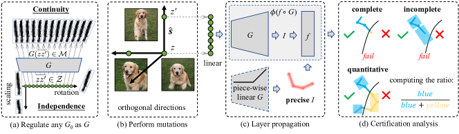
Figure 5: Overview of GCert. We illustrate the offline generative model regulation in (a), and the online input mutation and certification in (b)-(d).

Fig. 5 depicts the workflow of using GCert in NN certifications. Below, we first discuss the offline and online phases in Fig. 5. We then analyze six key benefits of GCert in –.

Offline Model Regulation: As in Fig. 5(a), given a common generative model $G_{o}$, we regulate $G_{o}$ with slight retraining. The “regulation” aims to satisfy two requirements: independence and continuity, as noted in Sec. 5 (see Sec. 5.1 and Sec. 5.2 for the technical details and correctness proof). The outcome of this phase is a regulated $G$, such that when moving an image’s latent point $z$ in $G$’s latent space, 1) distinct semantics are mutated independently, and 2) the mutated semantics in images $G(z)$ change continuously with $z$.

Online Input Mutations: By mutating a latent point $z$ along various orthogonal directions (due to independence) in the latent space of $G$, different semantic-level mutations are achieved unifiedly (benefit and ; see below). Also, as shown in Fig. 5(b), given a mutation and its corresponding direction $\hat{\bm{s}}$ (i.e., a unit vector) in the latent space, latent points corresponding to all mutated inputs are exclusively subsumed by a segment $\overline{zz^{\prime}}$ (where $z^{\prime}=z+\delta_{\max}\cdot\hat{\bm{v}}$) in the latent space due to continuity. $G(z)$ is the original image and $G(z^{\prime})$ is the mutated image with the maximal extent.

Online Layer Propagation: As in Fig. 5(c), the segment $\overline{zz^{\prime}}$ is propagated through $G$ to $f$ (our target NN) when conducting certification. Since $\overline{zz^{\prime}}$ (i.e., the input space of $f\circ G$) is linear, existing complete certifications $\phi$ (which require linear input space) can be directly applied on the new NN $f\circ G$ as $\phi(f\circ G(\overline{zz^{\prime}}))$. Moreover, when $G$ is piece-wise linear, a precise input space $I$ of $f$ can be obtained with only polynomial overhead (benefit ). This precise input space, with different forms (e.g., per-pixel lower/upper bound as in [11]), can be directly processed by existing certification frameworks.

Certification Analysis: When the online certification propagation is done, complete/incomplete (depending on if the layer propagation during certification is complete or not) certification can be conducted to assess the robustness of $f$. Since the input to $G$ is a segment, the output of $f$ will be a chain of segments (some “segments” may be over-approximated as box/polyhedra [46]). This representation enables quantitative certification (see benefit ).

Requirement of $G_{o}$ and Training Data. GCert does not require a special type of generative model $G_{o}$, and it converts $G_{o}$ into a regulated form $G$ automatically (see Sec. 5 and Sec. 6). We evaluate GCert on common generative models in Sec. 7.1. Also, $G$ has no special requirement on training data; we evaluate a set of common training datasets in Sec. 7.1. See Sec. 8 for further discussion on extensibility.

Key Benefits. GCert offers the following benefits:

 Advanced Mutation. GCert novelly enables certifying NNs under advanced mutations listed in Fig. 2. These mutations are rarely studied before, since they do not have explicit math expression and are usually arbitrary: they can easily introduce undesired perturbations which are hard to characterize. Sec. 5 explains how these problems are overcome.

 Unified Formulation. Following , GCert formulates various semantic-level mutations in Fig. 2 unifiedly: each mutation is denoted using one direction in the latent space of $G$. Then, mutating an image $x$ is achieved by moving the corresponding point $z$ along the direction in the latent space. The correctness of this unified formulation is studied in Sec. 5.1. Compared with prior certification frameworks considering one or a few specific mutations, extending GCert to take into account new mutations is straightforward; see Sec. 8.

 Practical Complete Certification over $f\circ G$. Since existing approaches cannot form a precise input space representation for semantic-level mutations, these mutations are never adopted by prior complete certifications. We view this as a major, yet rarely discussed threat to NNs, as semantic-level mutations generate images frequently encountered in reality, and they have been extensively studied in NN testing [50, 65]. GCert empowers complete certification with semantic-level mutations by applying complete certification on $f\circ G$ (see results in Sec. 7.2). The key solution is to use linear segment $\overline{zz^{\prime}}$ as the input for certifying $f\circ G$. While it appears that we add “extra burden” of certification by adding $G$, our enabled segment representation is however more efficient than prior “region” representation [66, 60, 20, 61]. Specifically, given a NN having $L$ layers and $N$ neuron width (which is much larger than $L$), our strategy reduces the cost from exponential $O((2^{N})^{L})$ [41] to $O((N^{2})^{L})$, which is polynomial when $L$ is fixed [57]; see analysis in Appx. B.

 Precise Input Space $I$ over $f$. An important conclusion, as noted by Sotoudeh et al. [57], is that given a piece-wise linear NN (e.g., ReLU as the activation function), if all of its inputs can be exclusively represented by a segment, then all of its output can also be exclusively represented as a chain of segments. This way, the input space $I$ of $f$ can be precisely represented. Following , the cost of computing precise input space representation is polynomial if $G$ has a fixed number of layers, which is true since $G$ does not add layers during the certification stage. Sec. 7.2.1 gives the cost evaluation. Existing certification frameworks, by using our precise input space (with different forms), can be smoothly extended to certify inputs mutated by semantic-level mutations. Sec. 7.2.1 compares previous (imprecise) SOTA input space with ours.

 Enabling Quantitative Certification. Complete certification can derive the maximum tolerance of NN $f$ to a mutation [32, 61]. However, the NN may still retain its correct prediction for some mutated inputs out of the maximum tolerance, as shown in Fig. 5(d). Quantitative certification provides fine-grained analysis by bounding the ratio of mutated inputs whose derived predictions are consistent [46]. The key idea is to represent all NN outputs as a chain of segments (see Fig. 5(d)). Then, quantitative certification is recast to computing the ratio of line segments that lie on the proper side of the decision boundary. Recall as in , the output of $f$ under GCert-involved certification has already been a chain of line segments. Thus, quantitative certification over various semantic-level mutations can be novelly enabled. Sec. 7.2.3 and Sec. 7.2.5 evaluate quantitative certification.

 Aligned Optimization in Incomplete Certification. In case where cost is the main concern, incomplete certification is more preferred, whose cost is $O(NL)$ [41]. That said, certification (formal verification) is inherently costly. One key objective in incomplete certification tasks is to tune the trade-off between precision vs. speed, by optimizing both input space representation and layer propagations. Nevertheless, the two optimizations are performed separately [11, 41], and in most cases, techniques in enhancing one optimization cannot be leveraged to boost the other. In contrast, note that GCert implements semantic-level mutations via $G$. Hence, incomplete certification integrated with GCert, when optimizes layer propagation of $f\circ G$, indeed covers both input space representation and layer propagation, in a unified manner.

5 Approach

Problem Formulation. In accordance with semantic-level mutations listed in Fig. 2, including all complex ($M_{c}$) and advanced ($M_{a}$) mutations, our unified mutation is as follows.

Definition 1 (Mutation).

Suppose $z\in\mathcal{Z}$ is the latent point of an image $x\in\mathcal{M}$, mutating $x$ as $x^{\prime}$ using semantic-level mutations can be conducted via a generative model $G$

$$\small x^{\prime}=G(z+\|\delta\|\cdot\hat{\bm{s}}_{\tau}),$$ (2)

where $\hat{\bm{s}}_{\tau}$ is a unit vector (i.e., $\left\lVert\hat{\bm{s}}_{\tau}\right\rVert=1$) that specifies the direction of one semantic-level mutation $\tau$. The norm of $\delta$, $\|\delta\|$, decides to what extent the mutation is performed.

As in Sec. 3, to support NN certification, we require the mutation in Def. 1 to satisfy the following two requirements.

$\bullet$ Independence: When moving $z$ in the latent space $\mathcal{Z}$ along $\hat{\bm{s}}_{\tau}$, the resulting image should only change semantics associated to $\tau$. For instance, mutating a portrait’s eyes (e.g., by making them close) should not affect its gender.

$\bullet$ Continuity: Mutated semantics must change continuously with $\|\delta\|$, such that points in segment $\overline{zz^{\prime}}$ that connects $z$ and $z^{\prime}=z+\|\delta_{\max}\|\cdot\hat{\bm{s}}_{\tau}$, when being used to generate images, comprise exclusively all “intermediate images” between $G(z)$ and $G(z^{\prime})$. For instance, if $G(z^{\prime})$ rotates $G(z)$ for $30^{\circ}$, $G(\overline{zz^{\prime}})$ should include all rotated $G(z)$ within $30^{\circ}$ and no others.

Sec. 5.1 and Sec. 5.2 show how these two requirements are achieved. In Sec. 5.3, we prove how they ensure the soundness and completeness of certification.

5.1 Achieving Independence

As an intuition, we first explore, when moving $z$ in the latent space, what decides the mutated semantics.

Definition 2 (Taylor Expansion).

Given a generative model $G$, for each $z$ and an infinitesimal $\Delta z$, according to Taylor’s theorem, we can expand it as:

$$G(z+\Delta z)-G(z)=\mathbf{J}(z)\Delta z+O(\Delta z),$$ (3)

where $\mathbf{J}(z)$ is the local Jacobian matrix of $z$. Its $(i,j)$-th entry is $\mathbf{J}(z)_{i,j}=\frac{\partial G(z)_{i}}{\partial z_{j}}$, which is decided by $G$’s gradient calculated on $z$. $O(\Delta z)$ approaches zero faster than $\Delta z$.

The expansion in Eq. 3 suggests that for perturbations over $z$, the changed semantics of the generated image are governed by the Jacobian matrix $\mathbf{J}(z)$ over $z$. We then show how to decompose mutating directions from $\mathbf{J}(z)$.

Theorem 1 (Degeneration [19]).

Let the dimensionality of $\mathcal{Z}$ be $d$ and $\mathbf{J}^{(k)}$ be the Jacobian matrix of the input for the $k$-th layer of $G$. $\mathbf{J}^{(k)}$ is progressively degenerated with $k$:

$$\mathrm{rank}({\mathbf{J}^{(k+1)}}^{\intercal}\mathbf{J}^{(k+1)})\leq\mathrm{rank}({\mathbf{J}^{(k)}}^{\intercal}\mathbf{J}^{(k)})\leq d$$ (4)

where $\mathrm{rank}(\cdot)$ denotes the rank of a matrix.

Theorem 1 suggests that, when moving $z$ in $\mathcal{Z}$, not all dimensions of $\mathcal{Z}$ can lead to semantic changes of $G(z)$, because the rank of $\mathbf{J}^{\intercal}\mathbf{J}$ may decrease during the forward propagation in $G$. Thus, directly decomposing mutating directions over $\mathbf{J}$ is inapplicable [77]. Therefore, to enable semantic-level mutations as in Def. 1, we need to identify dimensions in $\mathbf{J}$ that correspond to effective mutations. Following [77], we perform Low-Rank Factorization (LRF) for the $\mathbf{J}^{\intercal}\mathbf{J}$ over $\mathcal{Z}$.

Solution. The LRF factorizes $\mathbf{J}^{\intercal}\mathbf{J}$ as $\mathbf{J}^{\intercal}\mathbf{J}=\mathbf{R}^{*}+\mathbf{E}^{*}$, where $\mathbf{R}^{*}$ is the low-rank matrix associated with effective semantics-level mutations, and $\mathbf{E}^{*}$ is the noise matrix. The rank of $\mathbf{R}^{*}$, $\mathrm{rank}(\mathbf{R}^{*})=r\leq d$ where $d$ is the dimensions of $\mathcal{Z}$, denotes the number of (independent) mutating directions (which is affected by the training data of the generative model $G$; see Sec. 7.1). Thus, it becomes clear that to mutate each semantic independently, we can apply singular value decomposition (SVD) for $\mathbf{R}^{*}$:

$$\mathbf{U},\bm{\Sigma},\mathbf{V}^{\intercal}=\mathrm{SVD}(\mathbf{R}^{*}),$$ (5)

where $\mathbf{V}=[\hat{\bm{v}}_{1},\dots,\hat{\bm{v}}_{r},\dots,\hat{\bm{v}}_{d}]$ is a concatenation of orthogonal vectors. Each $\hat{\bm{v}}$ is a unit vector corresponding to one semantic-level mutation. Since different $\hat{\bm{v}}$ are orthogonal, performing one mutation will not move $z$ towards other mutating directions. Therefore, we can independently mutate different semantics by setting $\hat{\bm{s}}$ in Eq. 2 as one vector from the first $r$-th vectors from $\mathbf{V}$ (as displayed in Eq. 6). The remaining $d-r$ vectors in $\mathbf{V}$ do not lead to semantic changes [77]. These non-mutating directions enable independent local mutations; see Sec. 5.4 for details.

$$x^{\prime}=G(z+\|\delta\|\cdot\hat{\bm{v}}),\quad\hat{\bm{v}}\in[\hat{\bm{v}}_{1},\dots,\hat{\bm{v}}_{r}].$$ (6)

5.2 Achieving Continuity

As in Sec. 3, $G(\mathcal{Z})$ constructs the manifold $\mathcal{M}$ which encodes semantics of images. Continuity requires the constructed $\mathcal{M}$ to be continuous. We define continuity in Def. 3 below.

Definition 3 (Continuity).

Suppose the distance metrics on $\mathcal{Z}$ and $\mathcal{M}$ are $l_{\mathcal{Z}}$ and $l_{\mathcal{M}}$, respectively. Then, $\forall z,z^{\prime}\in\mathcal{Z}$, $\mathcal{M}$ is continuous iff it satisfies

$$\frac{1}{C}\,l_{\mathcal{Z}}(z,z^{\prime})\;\leq\;l_{\mathcal{M}}(G(z),G(z^{\prime}))\;\leq\;C\,l_{\mathcal{Z}}(z,z^{\prime}),$$ (7)

where $C$ is a constant. The left bound ensures that different $z$ on $\mathcal{Z}$ induce non-trivial changes of semantics. The right bound guarantees that the semantic changes continuously with $z$. $l_{\mathcal{Z}}$ can be computed as the Euclidean distance between two points in the latent space. $l_{\mathcal{M}}$ denotes the semantic-level similarity and is an implicit metric.

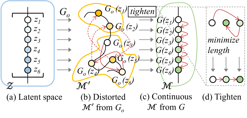
Figure 6: A schematic view of achieving continuity. The black lines ($-$) in (a)-(c) represent the intermediate points between two marked points. When mutating a point $z_{i}$, the red arrow ($\rightarrow$) in (b)-(d) marks the direction of changed $G_{o}(z_{i})$ and $G(z_{i})$. (a) depicts the latent space and the segment $\overline{z_{1}z_{6}}$ has intermediate points $z_{2}$-$z_{5}$. (b) shows a distorted $\mathcal{M}_{o}$, where $G_{o}(z)$ do not change continuously with $z$ and heavy distortion occurs. In (b), $G_{o}(z_{3})$ is the minimally mutated one among all marked points, and the dashed red arrow ($\dashrightarrow$) indicates an infinite length (as they cross two distorted sub-spaces scoped in yellow). (c) presents a continuous $\mathcal{M}$, where $G(z)$ yields gradual change with $z$, i.e., $G(z_{1})$ and $G(z_{6})$ denote the minimally and maximally mutated images, respectively. (d) illustrates the tightening procedure, which minimizes the length of red arrows ($\rightarrow$), thereby ensuring the continuity.

Fig. 6(b) shows a non-continuous $\mathcal{M}$ constructed by an “out-of-the-box” generative model $G_{o}$, where heavy distortions occur on $G_{o}(z)$ when $z$ changes slightly. That is, there are often sharp changes on the semantics between $G_{o}(z_{i})$ and $G_{o}(z_{i+1})$ though $z_{i}$ and $z_{i+1}$ stay close. To make $\mathcal{M}$ continuous, our intuition is to “tighten” it: $\forall z,z^{\prime}\in\mathcal{Z}$, and for all latent points in $\overline{zz^{\prime}}$, we minimize the length of the curve (which lies in $\mathcal{M}$) covered by all points in $G(\overline{zz^{\prime}})$. A schematic view of this tightening is in Fig. 6(d). The output would be a regulated $G$, whose $\mathcal{M}$ is continuous, as in Fig. 6(c). The following shows how a curve can be represented and how to calculate curve length by integrating its speed.

Definition 4 (Curve Length).

A curve connecting $a,a^{\prime}\in\mathcal{A}$ is denoted as the trajectory of a point when it moves from $a$ to $a^{\prime}$. It is formally represented as a mapping from a time interval to the space $\mathcal{A}$, along which the point moves:

$$\gamma_{\mathcal{A}}(t):[0,t]\rightarrow\mathcal{A},$$ (8)

where $\gamma_{\mathcal{A}}(t=0)=a$ and $\gamma_{\mathcal{A}}(t=T)=\overline{aa^{\prime}}$. Accordingly, the length of a curve can be calculated as:

$$\mathrm{Len}[\gamma_{\mathcal{A}}(T)]=\int_{0}^{T}\|\dot{\gamma}_{\mathcal{A}}(t)\|\mathrm{d}t,$$ (9)

where $\dot{\gamma}_{\mathcal{A}}(t)=\frac{\mathrm{d}\gamma_{\mathcal{A}}(t)}{\mathrm{d}t}$ is the point’s velocity at time $t$.

Problem Recast. Let $z_{t}$ be $z$’s location on $\mathcal{Z}$ at time $t$. Then, $\gamma_{\mathcal{Z}}(T)=\overline{z_{t=0}\,z_{t=T}}$ and $\gamma_{\mathcal{M}}(T)=G(\overline{z_{t=0}\,z_{t=T}})=G(\gamma_{\mathcal{Z}}(T))$. We can thus compute the length of $\gamma_{\mathcal{M}}(T)$ as:

$$\mathrm{Len}[\gamma_{\mathcal{M}}(T)]=\int_{0}^{T}\left\lVert\frac{\partial G\circ\gamma_{\mathcal{Z}}(t)}{\partial\gamma_{\mathcal{Z}}(t)}\frac{\partial\gamma_{\mathcal{Z}}(t)}{\partial t}\right\rVert\mathrm{d}t.$$ (10)

Suppose $\Delta t=\frac{T}{N}$ be an infinitesimal and $\gamma_{\mathcal{Z}}(\Delta t)=\Delta z$. Let $t_{i}=i\Delta t$, then, the length in Eq. 10 is reformulated as:

$$\mathrm{Len}[\gamma_{\mathcal{M}}(T)]=\sum_{i=0}^{N}\left\lVert\mathbf{J}(z_{t_{i}})\frac{\Delta z}{\Delta t}\right\rVert\Delta t=\sum_{i=0}^{N}\left\lVert\mathbf{J}(z_{t_{i}})\Delta z\right\rVert.$$ (11)

According to the Taylor expansion in Def. 2, we have

$$\|G(z_{t_{i}}+\Delta z)-G(z_{t_{i}})\|=\|\mathbf{J}(z_{t_{i}})\Delta z\|,$$ (12)

Therefore, $\gamma_{\mathcal{M}}(T)$’s length in Eq. 10 can be calculated as

$$\mathrm{Len}[\gamma_{\mathcal{M}}(T)]=\sum_{i=0}^{N}\left\lVert G(z_{t_{i}}+\Delta z)-G(z_{t_{i}})\right\rVert,$$ (13)

which is determined by the norm of $\mathbf{J}$.

Solution. The above recast for $\mathrm{Len}[\gamma_{\mathcal{M}}(T)]$ shows that, we can minimize $\|\mathbf{J}(z)\|>0$ for each $z$ to make $\mathcal{M}$ continuous. Meanwhile, we should align the starting and end points on two curves in $\mathcal{Z}$ and $\mathcal{M}$, i.e., $\gamma_{\mathcal{M}}(0)=G(\gamma_{\mathcal{Z}}(0))$ and $\gamma_{\mathcal{M}}(T)=G(\gamma_{\mathcal{Z}}(T))$. Inspired by the optimization objective in [52], we first define a monotonic function $\eta(\cdot)$ that satisfies $\eta(0)=0$ and $\eta(T)=1$. Then, for each $t_{i}=i\Delta t$, we add an extra regulation term as in the following Eq. 14 during the training stage of $G$. Overall, this regulation minimizes the distance between $G(z_{T})$ and $G(z_{0})$. Simultaneously, it forces $G(z_{t_{i}})$ to stay close to $G(z_{T})$ if $z_{t_{i}}$ is close to $z_{T}$, and vice versa for $z_{0}$ and $G(z_{0})$. As noted, the regulation term is agnostic to how the generative model is implemented or trained; it can be applied on any generative model.

$$\operatorname*{arg\,min}\limits_{\theta}\|\eta(t_{i})G_{\theta}(z_{T})-G_{\theta}(z_{t_{i}})-(1-\eta(t_{i}))G_{\theta}(z_{0})\|$$ (14)

Eq. 14 guarantees the continuity defined in Eq. 7; we provide detailed proof in Appx. A.

Distribution of latent space: $\mathcal{N}$; // Normal or uniform.

1

2function $Loss$($G_{o}$, $\mathcal{N}$, $\dots$):

       // The original training loss function of $G_{o}$ which returns a loss value.

3      

4function $Continuity$($G_{o}$, $\mathcal{N}$):

5       $z_{0}\sim\mathcal{N}$;   $z_{T}\sim\mathcal{N}$;

6       $\lambda\sim[0,1]$;   $z_{t_{i}}\leftarrow z_{0}+\lambda(z_{T}-z_{0})$;

7       return $\|\lambda G_{o}(z_{T})-G_{o}(z_{t_{i}})-(1-\lambda)G_{o}(z_{0})\|$;

8      

9function $Regulating$($G_{o}$, $\mathcal{N}$, $\dots$):

10       for $i\leftarrow 0$ to $\#epochs$ by $1$ do

11             $L_{1}\leftarrow Loss(G_{o},\mathcal{N},\dots)$;

12             $L_{2}\leftarrow Continuity(G_{o},\mathcal{N})$;

             // Optimize $G$ by minimizing $L_{1}+L_{2}$.

13            

14      return Regulated $G$;

15      

Algorithm 1 Regulating $G_{o}$ with continuity.

The procedure to regulate a generative model is in Alg. 1, where line 7 is the entry point. Eq. 14 serves as an extra loss term, which is added with the original training loss for optimization during the training stage (line 10). The monotonic function $\eta(\cdot)$ in Eq. 7 helps avoid sampling many points: in each training iteration, we randomly sample two points $z_{0}$, $z_{T}$ (line 4) and one point in-between as $z_{t_{i}}=z_{0}+\lambda(z_{T}-z_{0})$ (line 5). $\eta(t_{i})=\frac{t_{i}}{T}=\lambda$ helps $G(z_{t_{i}})$ stay in the shortest path connecting $G(z_{0})$ and $G(z_{T})$ (line 6). Regulating generative models with continuity should not harm their generation capability, since the original training objective is kept (line 9) during regulating. Moreover, continuity aims to “re-organize locations” of latent points (shown in Fig. 6) and the left bound in Eq. 7 ensures different $G(z)$ are generated with different $z$.

5.3 Soundness and Completeness Analysis

1 The target NN: $f$;   An input image: $x$ ;

2 The regulated generative model: $G\leftarrow Regulating(G_{o},\dots)$;

3 A certification framework: $\phi$;

// $\phi$ can be complete, incomplete, or quantitative.

$z\leftarrow G^{-1}(x)$; // Get the corresponding $z$ of $x$.

// Then get one mutating direction $\hat{\bm{s}}$ from $\mathbf{J}(z)$.

4 $z^{\prime}\leftarrow\|\delta_{\max}\|\cdot\hat{\bm{s}}$;

5if  or or  then

       $out\leftarrow\phi(f\circ G(\overline{zz^{\prime}}))$; // Optimize $f\circ G$’s propagations.

6      

7else if  then

       $I\leftarrow G(\overline{zz^{\prime}})$; // Precise $I$ if $G$ is piece-wise linear.

8       $out\leftarrow\phi(f(I))$;

       // Works for complete/incomplete/quantitative $\phi$.

9      

// Analyze $out$ according to $\phi$.

Algorithm 2 Certification with GCert.

Certifying NN robustness with GCert is given in Alg. 2. We demonstrate how GCert, which provides $G$ (line 2; see Alg. 1 for function $Regulating$) and $\overline{zz^{\prime}}$ (line 4-5), is incorporated into conventional certification framework $\phi$ under scenarios discussed in - of Sec. 4.

Below, we analyze the soundness and completeness. Overall, as in line 7 and line 10, the whole certification procedure with GCert can be represented as $\phi(f\circ G(\overline{zz^{\prime}}))$, where $\overline{zz^{\prime}}$ includes the corresponding latent points of all mutated inputs. To ease the presentation, we also use the term “sound” and “complete” for $\overline{zz^{\prime}}$. $\overline{zz^{\prime}}$ is sound if it does not miss any mutated input; it is complete if it only includes mutated inputs.

Lemma 1.

A certification $\phi(f\circ G(\overline{zz^{\prime}}))$ is sound iff both $\phi$ and $\overline{zz^{\prime}}$ are sound; it is complete iff both $\phi$ and $\overline{zz^{\prime}}$ are complete.

Proof. For a sound (but incomplete) $\phi$, the layer propagation in $f\circ G$ is progressively over-approximated (e.g., via abstract interpolation-based certification $\phi$ [22]). Since any mutated inputs will not be missed during the propagation, $\phi(f\circ G(\overline{zz^{\prime}}))$ is sound if $\overline{zz^{\prime}}$ is sound. For a complete (and sound) $\phi$, the layer propagation in $f\circ G$ is precisely captured (e.g., via symbolic execution-based certification $\phi$ [60]). Because the propagation does not introduce any new input, $\phi(f\circ G(\overline{zz^{\prime}}))$ is complete if $\overline{zz^{\prime}}$ is complete.

Since we use conventional sound and/or complete $\phi$, based on Lemma 1, the soundness and completeness of $\phi(f\circ G(\overline{zz^{\prime}}))$ is only decided by $\overline{zz^{\prime}}$. In the following, we analyze the soundness and completeness of $\overline{zz^{\prime}}$.

Soundness. The soundness of $\overline{zz^{\prime}}$ is ensured by the continuity: if $I$ misses some mutated inputs, there must exist two different $z_{1}$ and $z_{2}$ satisfying $G(z_{1})=G(z_{2})$, which violates continuity as defined in Eq. 7.

Completeness. The completeness of $\overline{zz^{\prime}}$ is ensured by both continuity and independence. With independence, different mutations are represented as orthogonal directions in the latent space. This way, performing one mutation will not move the latent point towards other unrelated directions. Also, when doing local mutations within one region, the mutating direction is projected into the non-mutating direction of other unrelated regions (see Eq. 17), such that only semantics over the specified region are mutated. For continuity, if an undesirable input (which is not generated by the mutation) appear in $\overline{zz^{\prime}}$, for the corresponding latent point $z^{*}$, there exists $z^{*}+\epsilon$ (where $\epsilon\rightarrow 0$ is an infinitesimal), such that $\|G(z^{*})-G(z^{*}+\epsilon)\|>C\epsilon$, which contradicts the definition in Eq. 7.

5.4 Unified Semantic-Level Mutations

This section shows how semantic-level mutations, including geometrical, stylized, global perceptual, and local perceptual mutations, are implemented uniformly.

5.4.1 Local Perceptual Mutations

To enable local perceptual mutations for one specific region $F$ (e.g., the eyes in Fig. 2), our intuition is to identify a direction in $\mathcal{Z}$ towards which $F$ can be mutated, whereas other regions are unchanged. Recall that in Sec. 5.1, LRF produces a set of non-mutating vectors which do not lead to mutations (i.e., $[\hat{\bm{v}}_{r+1},\dots,\hat{\bm{v}}_{d}]$ derived from Eq. 5). Thus, local perceptual mutations over $F$ can be performed by first project $F$’s mutating directions into the non-mutating vectors of the remaining region. To ease the presentation, let’s divide an image as foreground, which is the mutated region $F$, and background, which includes the remaining unchanged regions. Let $\mathbb{P}_{x}$ be the set of all indices of $x$, then we have

$$\mathbb{P}_{x}=\mathbb{F}_{x}\cup\mathbb{B}_{x},\quad\emptyset=\mathbb{F}_{x}\cap\mathbb{B}_{x},$$ (15)

where $\mathbb{F}_{x}$ and $\mathbb{B}_{x}$ denote two sets of indices belonging to $F$ and background, respectively. As in Eq. 16, we first calculate the Jacobian matrix of $\mathbb{F}_{x}$:

$$\mathbf{J}^{\mathbb{F}}(z):\quad\mathbf{J}^{\mathbb{F}}(z)_{(i,j)}=\frac{\partial G(z)_{i}}{\partial z_{j}},\;i\in\mathbb{F}_{x}.$$ (16)

Following our solution in Sec. 5.1, we apply LRF and SVD on $\mathbf{J}^{\mathbb{F}}(z)$ to get the corresponding $\mathbf{V}^{\mathbb{F}}$, whose rank is $r_{\mathbb{F}}$. Then, by using $\mathbf{V}^{\mathbb{F}}$ as in Eq. 6, a total of $r_{\mathbb{F}}$ mutating directions for the foreground is obtained. Similarly, we repeat the same procedure for $\mathbb{B}_{x}$ and obtain $\mathbf{V}^{\mathbb{B}}=[\hat{\bm{v}}_{1},\dots,\hat{\bm{v}}_{r_{\mathbb{B}}},\dots,\hat{\bm{v}}_{d}]$, where the last $d-r_{\mathbb{B}}$ vectors do not lead to mutations over $\mathbb{B}$, i.e., the non-mutating vectors of the background.

Let $\mathbf{F}=[\hat{\bm{v}}_{1_{\mathbb{F}}},\dots,\hat{\bm{v}}_{r_{\mathbb{F}}}]\subset\mathbf{V}^{\mathbb{F}}$, and $\mathbf{B}=[\hat{\bm{v}}_{r_{\mathbb{B}}+1},\dots,\hat{\bm{v}}_{d_{\mathbb{B}}}]$. Then, before mutating foreground perceptions, we project each vector in $\mathbf{F}$ into $\mathbf{B}$ (see Eq. 17). This way, only perceptions over the region specified by $F$ are mutated.

$$x^{\prime}=G(z+\lambda\hat{\bm{s}}),\quad\hat{\bm{s}}=\mathbf{B}\mathbf{B}^{\intercal}\hat{\bm{v}},\quad\hat{\bm{v}}\in\mathbf{F}.$$ (17)

5.4.2 Geometrical and Global Perceptual Mutations

Geometrical mutations can be viewed as a special case of global perceptual mutations. Here, we first perform “data augmentation,” by randomly applying various geometrical mutations with different extents $\delta$ on images in the training dataset. Our generative model $G$ is then trained with the augmented training dataset. Note that we do not need to explore all possible $\delta$; the generative model can infer intermediate $\delta$ ($0\leq\|\delta\|\leq\|\delta_{\max}\|$) because the constructed $\mathcal{M}$ is continuous (Sec. 5.2). We also give empirical analysis in Appx. C.

When performing global perceptual (or geometrical) mutations, the whole image is treated as the “foreground.” Therefore, we can easily follow Eq. 6 to perform mutations and satisfy the independence and continuity requirements.

Clarification. Perceptual mutations are not arbitrary. As discussed in Sec. 3, generative models enable “data-driven” mutations — the perception changes, therefore, are naturally constrained by diverse perceptions in real-world data (which are used to train our generative model $G$). For example, an eye will not be mutated into a nose, since such unrealistic combinations of perceptions do not exist in real data. Empirical evidences are provided in Appx. C.

5.4.3 Stylized Mutations

Stylized mutations are widely implemented via generative models (e.g., CycleGAN [78, 31]) in an independent manner. In particular, one individual generative model corresponds to one style, and therefore, we only need to use our solution in Sec. 5.2 to ensure their continuity. Implementations of stylized mutations can be depicted as the following procedures.

Data Preparation. The training data of these generative models are collected from two “style domains” $\mathcal{A}$ and $\mathcal{B}$. For example, $\mathcal{A}$ consists of images taken on sunny days, while $\mathcal{B}$ contains images taken on rainy days. Similarly, $\mathcal{A}$ may likewise consist of natural images, whereas $\mathcal{B}$ contains artistic paintings. The images in $\mathcal{A}$ and $\mathcal{B}$ do not need to have identical content (e.g., taking photos for the same car under different weather conditions is not necessary).

Training Strategy. The training procedure is based on domain transfer and cycle consistency [78, 31]. In practice, two generators, $G_{\mathcal{A}\mathcal{B}}$ and $G_{\mathcal{B}\mathcal{A}}$, are involved in the training stage. $G_{\mathcal{A}\mathcal{B}}$ maps images from domain $\mathcal{A}$ to domain $\mathcal{B}$, while $G_{\mathcal{B}\mathcal{A}}$ performs the opposite. The cycle consistency, at the same time, requires $\forall a\in\mathcal{A},a=G_{\mathcal{B}\mathcal{A}}(G_{\mathcal{A}\mathcal{B}}(a))$, and vice versa. This allows the two generators to comprehend the difference between two style domains, enabling style transfer. It is worth noting that each $G$ takes an extra input $\delta$ to control to what extent the style is transferred.

Mutation & Certification. As explained before, each generator is only capable of performing mutations for a single style, hence different stylized mutations are naturally implemented in an independent way. Therefore, to incorporate stylized mutations into NN certification, it is only necessary to establish continuity. To do so, our regulation term in Eq. 14 is applied on $\delta$, as expressed below:

$$\operatorname*{arg\,min}\limits_{\theta}\|\eta(t_{i})G_{\theta}(a,\delta_{T})-G_{\theta}(a,\delta_{t_{i}})-(1-\eta(t_{i}))G_{\theta}(\delta_{0})\|,$$

where $\delta_{t_{i}}$ increases with $t_{i}$. The same applies for $G_{\mathcal{B}\mathcal{A}}$.

6 Implementation

We implement GCert in line with Sec. 5, including 1) the solutions for the two requirements, 2) various semantic-level mutations, 3) the support for different generative models, and 4) some glue code for various certification frameworks, with a total of around 2,000 LOC in Python. We ran experiments on Intel Xeon CPU E5-2683 with 256GB RAM and a Nvidia GeForce RTX 2080 GPU.

Piece-Wise Linear. As explained in Sec. 5, a piece-wise linear $G$ is required to obtain precise input space $I$ for $f$ with a polynomial cost. GCert is however not limited to piece-wise linear $G$. For instance, when performing incomplete (but sound) certifications (which do not require a precise $I$), $G$ can be any generative model after being regulated; existing certification frameworks can be directly applied on $f\circ G$. Note that the last layer of $G$ needs to convert its inputs from $x\in[-\infty,\infty]$ into $[0,1]$ or $[-1,1]$ to generate images of valid pixel values (as pixel values are rescaled into $[0,1]$ or $[-1,1]$ [7, 6]). In practice, this layer is often implemented with $Sigmoid(x):[-\infty,\infty]\rightarrow[0,1]$ or $Tanh():[-\infty,\infty]\rightarrow[-1,1]$ which are not piece-wise linear. Therefore, we re-implement $G$’s last layer (which does not affect its capability; see Sec. 7.1) using the piece-wise linear function $ReLU(x)=\max(x,0)$, as $ReLU(-ReLU(x)+1)$ for $[-\infty,\infty]\rightarrow[0,1]$ and $ReLU(-ReLU(x)+2)-1$ for $[-\infty,\infty]\rightarrow[-1,1]$.

7 Evaluation

Evaluations of GCert-enabled mutations are launched in Sec. 7.1. Then, Sec. 7.2 studies the input space representation of GCert  and incorporates GCert into different certification frameworks for various applications. We also summarize lessons we learned from the evaluations.

7.1 Mutations and Generative Models

Evaluation Goal. This section corresponds to and discussed in Sec. 4. It serves as the empirical evidence besides the theoretical analysis of correctness in Sec. 5. We first launch qualitative and quantitative evaluations to assess the correctness and diversity of various $G$-supported mutations. Due to the limited space, ablation studies of how $G$’s capability is affected are presented in Appx. C.

Table 1: Evaluated datasets and generative models.

Dataset	MNIST [16]	CIFAR10 [37]	CelebA [43]	CelebA-HQ [33]	Driving [3]
Size	32 $\times$ 32	32 $\times$ 32	64 $\times$ 64	256 $\times$ 256	256 $\times$ 128
Task	Classification		Face recognition		Auto driving
Color	Gray-scale	RGB
$G$	DCGAN* [51]	BigGAN [14]	WGAN* [10]	StyleGAN [34]	CycleGAN [78]

• * DCGAN/WGAN is configured as piece-wise linear following Sec. 6.

Datasets. Table 1 lists the used datasets. MNIST consists of images of handwritten digits with a single color channel. Images in other datasets are RGB images. CIFAR10 contains real-life images of ten categories and is typically adopted for classification. CelebA-HQ consists of human face photos of much larger size. Note that CelebA-HQ images have exceeded the capacity of contemporary certification frameworks. Nevertheless, we use CelebA-HQ to demonstrate that more fine-grained mutations can be enabled in GCert. Images of higher resolution generally support more fine-grained mutations. Driving consists of driving-scene images captured by a dashcam and is mostly used to predict steering angles using NNs. In sum, these datasets are representative.

Generative Models. We employ popular generative models listed in Table 1 (see implementation details in [1]). As introduced in Sec. 5, our enforcement of independence and continuity is agnostic to the implementation of generative models. We assess several commonly-used generative models to illustrate the generalization of our approach.

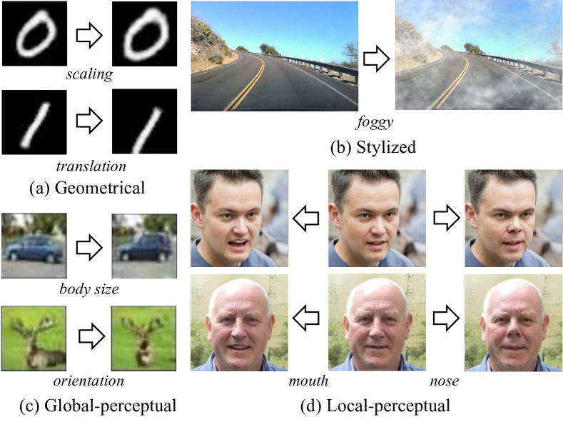
Figure 7: Independence evaluation. To clarify, CIFAR10 images in (c) generally have low resolution; GCert does not undermine its resolution.

7.1.1 Qualitative Evaluation

Independence. Fig. 7 shows images mutated using different type of mutations listed in Fig. 2. Compared with the original images, mutations enabled by GCert are independent. For example, in the lower case of Fig. 7(a), the translation scheme only changes the position of the digit, but retains the scale and the rotating angle. In the upper case of Fig. 7(d), when mutating the mouth, other facial attributes are unchanged.

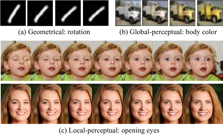
Figure 8: Continuity evaluation. To clarify, CIFAR10 images in (b) generally have low resolution; GCert does not undermine its resolution.

Continuity. Fig. 8 presents a sequence of changed images when gradually increasing $\delta$. Clearly, the mutated properties change continuously with $\delta$. Moreover, from Fig. 8(a), it is apparent that the rotation degree of the second image is bounded by the first (the original one) and the third images, despite that the digit is only slightly rotated when comparing the first and the third images.

7.1.2 Quantitative Evaluation

Correctness. Since it is challenging to obtain ground truth for stylized and perceptual mutations, to evaluate the correctness of mutations achieved by $G$, we focus on geometrical mutations. Ideally, we can first perform geometric mutations as ground truth, and then compare them with results of $G$ in a pixel-to-pixel manner. However, as mentioned in Sec. 2.2, geometrical mutations perform interpolations because pixel indexes are integers. Different interpolation algorithms will produce images of different pixel values, but the geometrical mutations are equivalent. Also, objects in images are irregular. As a result, obtaining their geometric properties (e.g., size, rotating angle) is challenging.

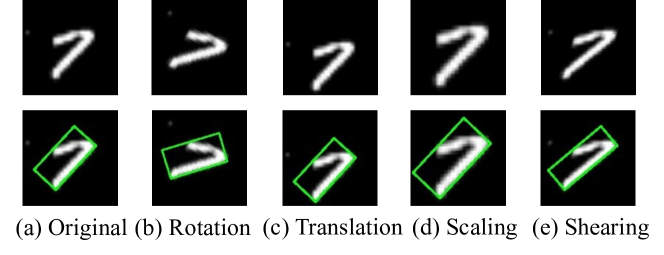
Figure 9: Minimum enclosing rectangles of objects.

Nevertheless, it is unnecessary to have the exact geometric properties, since we only need to check whether the geometric properties change independently and continuously. Therefore, we compute the minimum enclosing rectangle of an object, as shown in Fig. 9. We then check whether independence and continuity hold for geometric properties of this rectangle when the image is gradually mutated. In particular, to evaluate independence, we check whether other geometrical properties are unchanged when gradually mutating one geometrical property. Since shearing mutation warps the object horizontally or/and vertically, it will change the size and rotation angle of enclosing rectangle. Thus, it is infeasible to check the independence between shearing and scaling/rotation. As shown in Table 2, these mutations satisfy the independence.

To evaluate continuity, for each geometrical property, we first randomly generate two images $x_{1}$ and $x_{2}$ (by mutating $x_{1}$ as $x_{2}$) whose geometrical differences are $\Delta$ (e.g., the rotated angle is $30^{\circ}$). Then, for the corresponding latent points $z_{1}$ and $z_{2}$, we randomly sample points $z^{\prime}$ from the segment $\overline{z_{1}z_{2}}$. For every sampled point $z^{\prime}$, we obtain $x^{\prime}=G(z^{\prime})$ and check whether the geometrical difference between $x^{\prime}$ and $x_{1}$ (or $x_{2}$) is no greater than $\Delta$. We repeat both and for 100 times which results in total 10,000 checks. We checked $\Delta$ of different scales (i.e., $\Delta_{1}$ and $\Delta_{2}$ in Table 3). The passed check ratios for different geometrical mutations are reported in Table 3. Clearly, all points satisfy the continuity requirement.

Table 2: Quantitative evaluation for independence.

	Translation	Rotation	Scaling	Shearing
Translation	N/A	✓	✓	✓
Rotation	✓	N/A	✓	N/A
Scaling	✓	✓	N/A	N/A
Shearing	✓	N/A	N/A	N/A

• * ✓ means the mutation in the row does not influence the mutation in the column header.

Table 3: Quantitative evaluation for continuity*.

	Translation	Rotation	Scaling	Shearing
$\Delta_{1}$	100%	100%	100%	100%
$\Delta_{2}$	100%	100%	100%	100%

• * $\langle\Delta_{1},\Delta_{2}\rangle$ are $\langle\pm 10,\pm 4\rangle$, $\langle\pm 30^{\circ},\pm 10^{\circ}\rangle$, $\langle\pm 50\%,\pm 20\%\rangle$, $\langle\pm 10,\pm 4\rangle$ for translation, rotation, scaling, and shearing, respectively.

Diversity. Geometric mutations are of a fixed number, and each stylized mutation is separately implemented (i.e., one $G$ supports one style). Hence, we focus on evaluating the diversity of perceptual mutations. As discussed in Sec. 5.1, after performing LRF for the Jacobian matrix $\mathbf{J}$, the rank of the obtained low-rank matrix decides the number of independent mutations. For the CelebA-HQ dataset, the rank is around 35. Clearly, a considerable amount of perceptual mutations are enabled; see Appx. C for results of CIFAR10 ranks. We present more cases of perceptual mutations in our artifact [1].

7.2 Certification and Applications

Evaluation Goal. This section first collects the precise input space for various semantic-level mutations offered by GCert, and compares them with bounds yielded by previous approaches in Sec. 7.2.1 (i.e., in Sec. 4). Then, using different certification frameworks, we certify various NNs with semantic-level mutations in different scenarios.

Sec. 7.2.2 leverages GCert to perform complete certification and studies how NN architectures and training strategies affect its maximal tolerance to different mutations. Sec. 7.2.3 incorporates GCert into existing quantitative certification frameworks to certify perceptual-level mutations over face recognition. Sec. 7.2.4 conducts incomplete certification (which has the highest scalability) with GCert for autonomous driving. Sec. 7.2.5 systematically evaluates NN robustness towards all different types of mutations.

Table 4: Comparing average/median distances between lower and upper bounds yielded by GCert and DeepG.

Tool	Rotation $\pm 30^{\circ}$		Translation $\pm 4$		Precise∗
	Avg./Med. Distance	Speed	Avg./Med. Distance	Speed
DeepG	0.120/0.116	2.12s	0.144/0.146	2.57s	✗
GCert	0.075/0.076	0.16s	0.087/0.083	0.21s	✓

• * Whether the tool delivers a precise input space.

7.2.1 Precise Input Space

We compare GCert with the SOTA approach DeepG [11], a deterministic certification tool. As noted in Sec. 2.3, probabilistic approaches determine if the NN is robust with a probability. We deem this as undesirable, and thus omit comparison with probabilistic approaches. To offer a precise input space representation, GCert uses a piece-wise linear $G$ (DCGAN in Table 1) at this step. In contrast, SOTA approaches like DeepG over-approximate the input space.

Setup. Following DeepG, we first randomly select 100 images from the MNIST dataset. Then, for each image, we compute the precise input space resulted from rotation/translation (we follow the same setting as DeepG and configurations are listed in Table 4) using GCert, and obtain the upper/lower bounds for every pixel value. Finally, we compute the average distance between the upper and lower bounds, and compare the results with that of DeepG. To clarify, the precise input space representation yielded by GCert is not a set of lower/upper bounds. Instead, it is a chain of segments generated by the piece-wise linear $G$ in GCert. To use precise input space for certification, users directly pass the chain into the target NN for certification. Here, we compute the lower/upper-bound form over our generated chain to ease the comparison with DeepG, as it computes lower/upper bounds.

Results. As presented in Table 4. GCert reduces the average/median distances by around $40\%$ compared with DeepG. In addition, GCert’s speed should not be a concern. As reported in Table 4, GCert takes about 0.2s to analyze one image, compared to 2s for DeepG. Training $G$ — a one-time effort for all images — takes about 150s. However, we do not take credit from speed. We clarify that DeepG computes bounds for each pixel on CPUs in parallel while GCert executes on a GPU (i.e., a forward pass of $G$).

We also benchmark probabilistic certifications; we use TSS [42], the SOTA framework. Probabilistic certifications use the Monte Carlo algorithm to sample mutated inputs when estimating the input space, which is not aligned with the input space in deterministic certifications. Nevertheless, we report the time cost of sampling (on the same hardware with GCert) for reference. In practice, the time cost is mainly decided by the number of samples, for example, sampling 100K mutated inputs (following the default setup) takes 5–6s and only 0.05s is need if sampling 1K inputs. We interpret its speed is reasonable and comparable to that of GCert.

Table 5: NNs and their tolerance to different mutations.

	#Conv1	#FC1	#Layer	Aug.2	Speed	Max. R3	Max. T4	Max. S5
$f_{1}$	0	3	3	✗	0.98s	$41.1^{\circ}$	6.5	32%
$f_{2}$	2	1	3	✗	1.76s	$52.9^{\circ}$	7.6	39%
$f_{3}$	4	2	6	✗	3.86s	$72.3^{\circ}$	9.1	44%
$f_{4}$	4	2	6	✓	3.85s	$90.0^{\circ}$	9.3	51%

• 1. Conv is convolutional layer and FC is fully-connected layer.

• 2. Aug. flags whether the NN is trained with data augmentation, where during training, geometrical mutations are applied on the training data to increase the amount and diversity of training samples.

• 3. Max. R/T/S denotes the averaged maximal tolerance under rotation/translation/scaling where the NN consistently retains its prediction.

• 4. The numerical unit is pixel.

• 5. The tolerance $x\%$ denotes scaling within $[1-x\%,1+x\%]$.

7.2.2 Complete Certification for Classification

Setup. We perform complete certification for NNs listed in Table 5. These NNs are composed of different numbers/types of layers and trained with different strategies. They perform 10-class classification on the MNIST dataset. We certify their robustness using 100 images randomly selected from the test dataset of MNIST. GCert offers complete certification, meaning if the certification fails, the NN must have mis-predictions. For each image, we record the maximal tolerance (within which the NN retains its prediction) to different mutations. For each NN, we report the average tolerance over all tested images in Table 5. A higher tolerance indicates that the NN is more robust to the mutation. Since we require a meaningful metric to measure the tolerance, we focus on geometrical mutations which have explicit math expressions: the tolerance can be expressed using interpretable numbers. In this evaluation, GCert is bridged with ExactLine [57], a complete certification framework.

Conv vs. FC. As shown in Table 5, these NNs manifest different degrees of robustness towards various mutations. Comparing $f_{1}$ and $f_{2}$, we find that replacing FC with Conv layers can enhance the robustness. It is known that Conv, due to its sparsity, is more robust if the input image is seen from different angles (which is conceptually equivalent to rotation/translation/scaling) [38, 72]. Our results support this heuristic.

Depth. Comparing $f_{2}$ and $f_{3}$ reveals that increasing the depth (adding more layers) of NNs also enhances the robustness. According to prior research [55], deeper layers in NNs extract higher-level concepts from inputs, e.g., “digit 1” is a higher-level concept than “digit position.” Consequently, deeper NNs should be more resilient to perturbations that change low-level image concepts (which correspond to the primary effect of geometrical mutations). Our results justify this hypothesis from the certification perspective.

Data Augmentation. The tolerance increase of $f_{4}$ relative to $f_{3}$ shows the utility of data augmentation (by randomly performing geometrical mutations on training data) for enhancing robustness. Applying geometrical mutations on training data “teaches” the NN to not concentrate on specific geometrical properties (since these properties may have been diminished in the mutated training data). Previous works mostly use data augmentation to increase the accuracy of NNs since more data are used for training. Our evaluation offers a new viewpoint on the value of data augmentation.

Speed. Table 5 shows the time of analyzing one image in GCert. Though complete certification was believed costly, it is relatively fast in GCert: for the largest NNs ($f_{3}$ and $f_{4}$), one complete certification takes less than 4s. The main reason is that in previous complete certification, all inputs are represented as a region, whereas they are simplified as a segment to $f\circ G$ in GCert. We give detailed complexity analysis in Appx. B.

7.2.3 Quantitative Certification for Face Recognition

Besides incorporating GCert with complete certification, we use GCert for quantitative certification below.

Setup & Framework. We incorporate GCert into GenProver [46] for quantitative certification: it delivers more fine-grained analysis by computing the lower/upper bound for the percentage of mutated inputs that retain the prediction. The target NN takes two face photos as inputs and predicts whether they belong to the same person (i.e., predicts a number in $[0,1]$ to indicate the probability of being the same person). Given the rich set of global and local perceptions in human faces, we focus on perceptual-level mutations in this section. We first randomly select 100 pairs of face photos from CelebA (image size $64\times 64$), then, for each pair, we apply various global/local perceptual mutations (listed in Table 6) to one of the images. Then, we determine the lower and upper bounds of robustness (i.e., the percentage of inputs that will not change the prediction). In this setting, if the original prediction is “yes,” following GenProver, the computation for the lower/upper bounds is:

$$\text{Lower Bound}=\sum_{i}\lambda_{i}\,\bm{[}\,\forall q\in P_{i},q>0.5\,\bm{]}$$

$$\text{Upper Bound}=\sum_{i}\lambda_{i}\,\bm{[}\,\exists q\in P_{i},q>0.5\,\bm{]}$$

where $\bm{[}\cdot\bm{]}$ outputs $1$ if the input condition holds, and $0$ otherwise. $P_{i}$ is the $i$-th segment in outputs of the certified NN $f$ (recall that the input segment of $f\circ G$ is bent by non-linear layers in $G$ and $f$), and $\lambda_{i}$ is the weight of $P_{i}$ (i.e, the ratio of its length over the whole length). $q$ is a point in $P_{i}$. If the original prediction is “no,” users can replace $q>0.5$ as $q\leq 0.5$.

Table 6: Quantitative certification for face recognition.

	Global	Local
	Orientation	Hair	Eye	Nose
Upper Bound	100%	98.1%	69.7%	95.2%
Lower Bound	97.6%	95.0%	60.3%	90.3%

• 1. Orientation: change face orientation. 2. Hair: change hair color.

• 3. Eye: open/close eyes, or add glasses. 4. Nose: change nose size.

Results. As in Table 6, the lower/upper bounds vary with the mutated facial attributes. Notably, orientation is less effective to flip the prediction, as the NN does not rely on orientation to recognize a face in most cases. In contrast, mutating eyes is highly effective to deceive the NN. This is reasonable, as NNs often rely on key facial attributes, such as eyes, to recognize faces [40, 63]. Hence, closing eyes or adding glasses will cause NNs to lose crucial information.

7.2.4 Certifying Autonomous Driving

Setup & Framework. In this evaluation, we incorporate GCert into $\text{AI}^{2}$ [22] (i.e., ERAN [4]) to certify if the NN is robust under various severe weather conditions. This is a common setup to stress NN-based autonomous driving [74, 50], and NN’s robustness is ensured if it can retain its steering angle decisions under severe weather conditions. We use the “rainy” and “foggy” filters to simulate the effects of rain and fog. Note that that geometrical and perceptual-level mutations do not apply here, because the steering angle is tied to geometrical properties and the road is frequently altered when mutating perceptions: the ground truth steering decisions are changed by these mutations. We randomly select 500 images from the Driving dataset for mutation and report the percentage of successful certification (i.e., the NN is proved to retain its prediction) for three degrees of mutations, as in Table 7. While $\text{AI}^{2}$ performs incomplete certification, it has SOTA scalability, allowing it to efficiently certify large images (whose size is $256\times 128$) in the Driving dataset.

Table 7: Certification for autonomous driving over severe weather conditions. Results are % of successful certifications.

	Small	Medium	Heavy
Rainy	97.5%	80.3%	70.9%
Foggy	96.2%	75.2%	61.7%

Results. Table 7 presents the results. The extent of weather filter is controlled by a floating number weight within $[0,1]$ (see Sec. 5.4.3). To ease analysis, we discretize it into three degrees (0.2, 0.5, and 0.8) in Table 7. When heavy weather filters are applied to these images, a considerable number of certifications fail. This may be a result of the inconsistent predictions (true positive certification failures) or the over-approximation of layer-propagation performed in $\text{AI}^{2}$ (false positive certification failures). Besides, the “foggy” filter seems more likely to break consistent predictions of NNs. This is intuitive, because fog can easily decrease the “visibility” of the NN, and therefore, road details (e.g., the yellow road stripes) for making decisions may be missing.

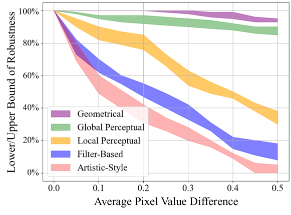
Figure 10: Compare different mutations in terms of lower/upper bounds.

7.2.5 Cross-Comparing Different Mutations

In this section, we study if the same NN has notably different robustness under different types of mutations. This step subsumes all mutations supported by GCert. For a more fine-grained measurement of the robustness, we incorporate GCert into GenProver for quantitative certification.

Dataset & NN. We use CelebA, as the resolution of CIFAR10/MNIST is insufficient for fine-grained local perceptual mutations. We still certify face recognition but for a ResNet [28], which is one highly successful and pervasively-used NN for computer vision tasks in recent years.

Setup. To compare the extent of these mutations in a unified way, we use the Average Pixel value Difference (APD):

$$\small APD=\frac{\sum_{i}|x_{i}-x_{i}^{\prime}|\,\bm{[}\,x_{i}\neq x_{i}^{\prime}\,\bm{]}}{\sum_{i}\bm{[}\,x_{i}\neq x_{i}^{\prime}\,\bm{]}}$$

where $x$ is the original image and $x_{i}$ is its $i$-th pixel. $x^{\prime}$ is the mutated image. $\bm{[}\cdot\bm{]}$ yields $1$ if $x_{i}\neq x_{i}^{\prime}$ and $0$ otherwise. Note that APD is only calculated over changed pixels to “normalize” the value, because geometrical and local-perceptual mutations do not change all pixels.

Results. Fig. 10 depicts how the lower/upper bounds of robustness change with varying APD values across different mutations. It is seen that for well-trained NNs like ResNet, geometrical mutation is not a major concern to impede its robustness: extensive geometrical mutations (when APD scores are high) can hardly flip predictions, as implied in Fig. 10. In contrast, stylized mutations, including both artistic-style and filter-based mutations, are effective at challenging NNs. This result is consistent to the recently-observed “texture-bias” in common NNs networks [23, 30]. In particular, people have observed that NNs heavily rely on texture to recognize objects, and that the predictions can be easily changed by mutating the texture (mostly by artistic-style transfer). Local-perceptual mutation has a major impact on the robustness as well. In contrast, global-perceptual mutation is less effective to stress the NNs. Recall that, as discussed in Sec. 7.2.3, NNs typically rely on key attributes (such as eyes) for predictions. While local-perceptual mutations like “closing eyes” stress the target NNs by changing those attributes, they are mostly retained in global-perceptual and geometrical mutations.

8 Discussion and Extension

In general, extending GCert can be conducted from the following aspects.

Mutations: GCert is data driven, in the sense that to add new semantic-level mutations, users only need to add images with new semantics to $G$’s training data. As evaluated in Appx. C, due to the continuity, GCert can infer “intermediate images” between the original and the mutated images without having them in the training data. According to our empirical observations, only dozens of data are enough to add one new mutation.

Data: Generative models have been widely adopted for generating data of various forms, such as text [75], audios [17]. GCert’s technical pipeline is independent of the implementation of generative models; therefore, GCert can support other data forms by employing the corresponding $G$.

Objectives/Tasks: GCert can boost certification of other NN tasks (e.g., object detection) and objectives (e.g., fairness), as those tasks also accept images as inputs and fit semantic-level mutations studied in this paper. For example, fairness certifications typically assess whether certain semantics (which are typically perceptual semantics such as gender) affect the NN prediction [59, 54]. GCert can boost them since it enables independent and analysis-friendly perceptual mutations. In short, despite the fact that supporting other tasks/objectives is not GCert’s main focus, such extensions should be straightforward, since GCert is not limited to particular certification techniques/objectives.

9 Conclusion

We have proposed GCert which enables the certification of NN robustness under diverse semantic-level image mutations. We identify two key properties, independence and continuity, that result in a precise and analysis-friendly input space representation. We show that GCert empowers de facto complete, incomplete, and quantitative certification frameworks using semantic-level image mutations with moderate cost, and under various real-world scenarios.

Appendix A Proof for Continuity (Eq. 7)

This section proves that continuity (Eq. 7) is satisfied, by regulating the generative model with Eq. 14 as in Alg. 1. Eq. 14 limits the gradients of $G$ over $z\in\mathcal{Z}$. As a result, $\|\mathbf{J}(z)\|$ is bounded. Suppose its maximum and minimum values are $A$ and $\frac{1}{B}$, respectively. For any path on $\mathcal{Z}$, namely, $\gamma_{\mathcal{Z}}(t):[0,t]\rightarrow\mathcal{Z}$, the length of the corresponding curve on $\mathcal{M}$ is

$$\mathrm{Len}(G(\gamma_{\mathcal{Z}}(T)))=\int_{0}^{T}\left\lVert\mathbf{J}(z_{t})\dot{\gamma}_{\mathcal{Z}}(t)\right\rVert\mathrm{d}t$$ (18)

Let $z$ and $z^{\prime}$ be the points at time $0$ and $T$, respectively. Since by design $\mathcal{Z}$ follows a continuous distribution, we have $\mathrm{Len}(\gamma_{\mathcal{Z}}(T))=l_{\mathcal{Z}}(z,z^{\prime})$. And therefore, the following inequation holds:

$$\mathrm{Len}(G(\gamma_{\mathcal{Z}}(t)))\leq A\int_{0}^{T}\left\lVert\dot{\gamma}_{\mathcal{Z}}(t)\right\rVert\mathrm{d}t=A\cdot l_{\mathcal{Z}}(z,z^{\prime}).$$ (19)

where $l_{\mathcal{Z}}(z,z^{\prime})$, the distance between $z$ and $z^{\prime}$, equals to the length of the shortest path connecting $z$ and $z^{\prime}$. Thus, we have

$$\frac{1}{B}\cdot l_{\mathcal{Z}}(z,z^{\prime})=\frac{1}{B}\int_{0}^{t}\left\lVert\dot{\gamma}_{\mathcal{Z}}(t)\right\rVert\mathrm{d}t\leq l_{\mathcal{M}}(G(z),G(z^{\prime}))$$ (20)

Similarly, since $l_{\mathcal{M}}(G(z),G(z^{\prime}))$ equals to the shortest length of the paths between $G(z)$ and $G(z^{\prime})$ on $\mathcal{M}$, we have $l_{\mathcal{M}}(G(z),G(z^{\prime}))\leq\mathrm{Len}(G(\gamma_{\mathcal{Z}}(t)))$.

Let $C=\max(A,B)$, the following equation thus holds:

$$\frac{1}{C}\cdot l_{\mathcal{Z}}(z,z^{\prime})\leq l_{\mathcal{M}}(G(z),G(z^{\prime}))\leq C\cdot l_{\mathcal{Z}}(z,z^{\prime}).$$ (21)

Besides the theoretical analysis, we also empirically calculate the value of $C$ (which $\geq 1$) over 10K inputs for generative models trained on different datasets. Results are in Table 8. We interpret the results as generally promising and intuitive.

Table 8: Values of $C$ in Eq. 7.

MNIST	CIFAR10	CelebA	Driving
2	5	3	3

Appendix B Cost Analysis

In practice, $f\circ G$ will typically double the number of layers (#layers) in $f$, as #layers is correlated with input image resolution: if $f$ is deeper (meaning its inputs exhibit higher resolution), then $G$ should also be deeper to generative more fine-grained images; the same holds true if $f$ is much shallower. As explained in Sec. 4, if $f$ has $L$ layers and $N$ neuron width (i.e., the maximum number of neurons in a layer), the conventional cost for complete certification is $O((2^{N})^{L})$ [41]. In GCert, the #layers of $f\circ G$ is approximately $2L$. Therefore, based on the results of [57], GCert’s cost is $O({N}^{2L})=O({({N}^{2})}^{L})$ — GCert reduces an exponential cost $O(2^{N})$ to a polynomial $O({N}^{2})$ for a given $L$. As evaluated in Table 4 and Table 5, GCert’s cost is empirically moderate.

Similarly, the cost for conventional incomplete certification is $O(NL)$ [41]. Since $f\circ G$ doubles the number of layers, GCert increases the certification cost to $O(2NL)$, which is still polynomial to neuron width and the number of layers.

Appendix C Ablation Studies

As mentioned in Sec. 3, $G$ enables “data-driven” mutations. Therefore, at this step we launch controlled experiments to explore how the training data of $G$ would affect the enabled mutations. More specifically, we study how the mutation quantity and extent are affected.

We observe that for CIFAR10 (image size is $32\times 32$), only approximately 2$\sim$4 global perceptual mutations can be identified. In comparison to the 35 global perceptual mutations in CelebA-HQ (image size is $256\times 256$), we interpret that the resolution of training images has a notable impact on the diversity of perceptual mutations. This is reasonable since, with a higher resolution, more details of perceptual contents can be modeled by the generative models.

In practice, it is infeasible to automatically decide if a specific perceptual mutation exists or to what extent it is applied. Thus, we focus on geometrical mutations in the following controlled experiments. Nevertheless, geometrical properties can be affected by diverse semantics in real datasets (e.g., a digit zero is written in different scales). To avoid such side effects, we construct a synthetic dataset of rectangle images (scripts are in [1]). In short, we first prepare a seed image which has one square with one-length sides (“a unit square”) at the center. We then apply different geometrical mutations over the seed to generate training data for $G$. This way, we can precisely control the number/extent of geometrical mutations involved in the training data.

We summarize the results as follows. First, the mutation supported by $G$ is not arbitrary: $G$ can only enable mutations whose mutated properties exhibit observed variations in the training data. Second, the maximal variation of the target property determines the largest extent (i.e., $\|\delta_{\max}\|$) of one mutation. More importantly, we emphasize that it is unnecessary to cover all possible $\|\delta\|$ values in the training data in order to enable all mutations within $\|\delta\|\leq\|\delta_{\max}\|$. Since $\mathcal{Z}$ follows a continuous distribution (introduced in Sec. 3) and $G$ satisfies the continuity (Sec. 5.2), only a few $\|\delta\|$ values within $\|\delta\|\leq\|\delta_{\max}\|$ need to be covered in the training data. This roots from the manifold hypothesis [12, 76] and demonstrates the merit of our generative model-based approach, as introduced in Sec. 3.

References

- [1] Artifact. https://github.com/Yuanyuan-Yuan/GCert.
- [2] Autonomous vehicle collision reports. https://www.dmv.ca.gov/portal/vehicle-industry-services/autonomous-vehicles/autonomous-vehicle-collision-reports/.
- [3] The driving dataset. https://github.com/SullyChen/driving-datasets.
- [4] Eran: Eth robustness analyzer for deep neural networks. https://github.com/eth-sri/eran.
- [5] Geometrical mutations in opencv. https://docs.opencv.org/4.x/da/d54/group__imgproc__transform.html.
- [6] Pytorch data processing. https://pytorch.org/vision/stable/transforms.html.
- [7] Tensorflow data processing. https://www.tensorflow.org/datasets/overview.
- [8] Tesla vehicle safety report. https://www.tesla.com/VehicleSafetyReport.
- [9] Motasem Alfarra, Adel Bibi, Naeemullah Khan, Philip HS Torr, and Bernard Ghanem. Deformrs: Certifying input deformations with randomized smoothing. In AAAI, volume 36, pages 6001–6009, 2022.
- [10] Martin Arjovsky, Soumith Chintala, and Léon Bottou. Wasserstein generative adversarial networks. In ICML, 2017.
- [11] Mislav Balunovic, Maximilian Baader, Gagandeep Singh, Timon Gehr, and Martin Vechev. Certifying geometric robustness of neural networks. Advances in Neural Information Processing Systems, 32, 2019.
- [12] Yoshua Bengio, Aaron Courville, and Pascal Vincent. Representation learning: A review and new perspectives. IEEE transactions on pattern analysis and machine intelligence, 35(8):1798–1828, 2013.
- [13] Gregory Bonaert, Dimitar I Dimitrov, Maximilian Baader, and Martin Vechev. Fast and precise certification of transformers. In PLDI, 2021.
- [14] Andrew Brock, Jeff Donahue, and Karen Simonyan. Large scale gan training for high fidelity natural image synthesis. In ICLR, 2018.
- [15] Patrick Cousot and Radhia Cousot. Abstract interpretation: a unified lattice model for static analysis of programs by construction or approximation of fixpoints. In Proceedings of the 4th ACM SIGACT-SIGPLAN symposium on Principles of programming languages, pages 238–252, 1977.
- [16] Li Deng. The mnist database of handwritten digit images for machine learning research. IEEE Signal Processing Magazine, 29(6):141–142, 2012.
- [17] Chris Donahue, Julian McAuley, and Miller Puckette. Adversarial audio synthesis. In ICLR, 2018.
- [18] Isaac Dunn, Hadrien Pouget, Daniel Kroening, and Tom Melham. Exposing previously undetectable faults in deep neural networks. In ISSTA, 2021.
- [19] Ruili Feng, Deli Zhao, and Zheng-Jun Zha. Understanding noise injection in gans. In ICML, 2021.
- [20] Claudio Ferrari, Mark Niklas Mueller, Nikola Jovanović, and Martin Vechev. Complete verification via multi-neuron relaxation guided branch-and-bound. In International Conference on Learning Representations, 2021.
- [21] Marc Fischer, Maximilian Baader, and Martin Vechev. Certified defense to image transformations via randomized smoothing. NeurIPS, 2020.
- [22] Timon Gehr, Matthew Mirman, Dana Drachsler-Cohen, Petar Tsankov, Swarat Chaudhuri, and Martin Vechev. Ai2: Safety and robustness certification of neural networks with abstract interpretation. In 2018 IEEE symposium on security and privacy (SP), 2018.
- [23] Robert Geirhos, Patricia Rubisch, Claudio Michaelis, Matthias Bethge, Felix A Wichmann, and Wieland Brendel. Imagenet-trained cnns are biased towards texture; increasing shape bias improves accuracy and robustness. In ICLR, 2018.
- [24] Ian Goodfellow, Patrick McDaniel, and Nicolas Papernot. Making machine learning robust against adversarial inputs. Communications of the ACM, 2018.
- [25] Ian Goodfellow, Jean Pouget-Abadie, Mehdi Mirza, Bing Xu, David Warde-Farley, Sherjil Ozair, Aaron Courville, and Yoshua Bengio. Generative adversarial networks. Communications of the ACM, 2020.
- [26] Ian J Goodfellow, Jonathon Shlens, and Christian Szegedy. Explaining and harnessing adversarial examples. stat, 1050:20, 2015.
- [27] Zhongkai Hao, Chengyang Ying, Yinpeng Dong, Hang Su, Jian Song, and Jun Zhu. Gsmooth: Certified robustness against semantic transformations via generalized randomized smoothing. In ICML, 2022.
- [28] Kaiming He, Xiangyu Zhang, Shaoqing Ren, and Jian Sun. Deep residual learning for image recognition. In CVPR, 2016.
- [29] Dan Hendrycks, Kevin Zhao, Steven Basart, Jacob Steinhardt, and Dawn Song. Natural adversarial examples. In CVPR, 2021.
- [30] Katherine Hermann, Ting Chen, and Simon Kornblith. The origins and prevalence of texture bias in convolutional neural networks. NeurIPS, 2020.
- [31] Phillip Isola, Jun-Yan Zhu, Tinghui Zhou, and Alexei A Efros. Image-to-image translation with conditional adversarial networks. In CVPR, 2017.
- [32] Matt Jordan, Justin Lewis, and Alexandros G Dimakis. Provable certificates for adversarial examples: Fitting a ball in the union of polytopes. NeurIPS, 2019.
- [33] Tero Karras, Timo Aila, Samuli Laine, and Jaakko Lehtinen. Progressive growing of gans for improved quality, stability, and variation. In ICLR, 2018.
- [34] Tero Karras, Samuli Laine, and Timo Aila. A style-based generator architecture for generative adversarial networks. In CVPR, 2019.
- [35] Diederik P Kingma and Max Welling. Auto-encoding variational bayes. stat, 1050:1, 2014.
- [36] Durk P Kingma and Prafulla Dhariwal. Glow: Generative flow with invertible 1x1 convolutions. Advances in neural information processing systems, 31, 2018.
- [37] Alex Krizhevsky, Geoffrey Hinton, et al. Learning multiple layers of features from tiny images. 2009.
- [38] Yann LeCun, Fu Jie Huang, and Leon Bottou. Learning methods for generic object recognition with invariance to pose and lighting. In Proceedings of the 2004 IEEE Computer Society Conference on Computer Vision and Pattern Recognition. IEEE, 2004.
- [39] Mathias Lecuyer, Vaggelis Atlidakis, Roxana Geambasu, Daniel Hsu, and Suman Jana. Certified robustness to adversarial examples with differential privacy. In IEEE S&P, 2019.
- [40] Haoxiang Li, Zhe Lin, Xiaohui Shen, Jonathan Brandt, and Gang Hua. A convolutional neural network cascade for face detection. In CVPR, 2015.
- [41] Linyi Li, Xiangyu Qi, Tao Xie, and Bo Li. Sok: Certified robustness for deep neural networks. In 2023 IEEE symposium on security and privacy (SP). IEEE, 2023.
- [42] Linyi Li, Maurice Weber, Xiaojun Xu, Luka Rimanic, Bhavya Kailkhura, Tao Xie, Ce Zhang, and Bo Li. Tss: Transformation-specific smoothing for robustness certification. In CCS, 2021.
- [43] Ziwei Liu, Ping Luo, Xiaogang Wang, and Xiaoou Tang. Deep learning face attributes in the wild. In ICCV, 2015.
- [44] Benjamin Livshits, Manu Sridharan, Yannis Smaragdakis, Ondřej Lhoták, J Nelson Amaral, Bor-Yuh Evan Chang, Samuel Z Guyer, Uday P Khedker, Anders Møller, and Dimitrios Vardoulakis. In defense of soundiness: A manifesto. Communications of the ACM, 2015.
- [45] Tobias Lorenz, Anian Ruoss, Mislav Balunović, Gagandeep Singh, and Martin Vechev. Robustness certification for point cloud models. In ICCV, 2021.
- [46] Matthew Mirman, Alexander Hägele, Pavol Bielik, Timon Gehr, and Martin Vechev. Robustness certification with generative models. In PLDI, 2021.
- [47] Jeet Mohapatra, Tsui-Wei Weng, Pin-Yu Chen, Sijia Liu, and Luca Daniel. Towards verifying robustness of neural networks against a family of semantic perturbations. In CVPR, 2020.
- [48] Mark Niklas Müller, Gleb Makarchuk, Gagandeep Singh, Markus Püschel, and Martin T Vechev. Prima: general and precise neural network certification via scalable convex hull approximations. POPL, 2022.
- [49] Mikhail Pautov, Nurislam Tursynbek, Marina Munkhoeva, Nikita Muravev, Aleksandr Petiushko, and Ivan Oseledets. Cc-cert: A probabilistic approach to certify general robustness of neural networks. In AAAI, 2022.
- [50] Kexin Pei, Yinzhi Cao, Junfeng Yang, and Suman Jana. Deepxplore: Automated whitebox testing of deep learning systems. In SOSP, 2017.
- [51] Alec Radford, Luke Metz, and Soumith Chintala. Unsupervised representation learning with deep convolutional generative adversarial networks. arXiv preprint arXiv:1511.06434, 2015.
- [52] Sameera Ramasinghe, Moshiur Farazi, Salman H Khan, Nick Barnes, and Stephen Gould. Rethinking conditional gan training: An approach using geometrically structured latent manifolds. NeurIPS, 2021.
- [53] Henry Gordon Rice. Classes of recursively enumerable sets and their decision problems. Transactions of the American Mathematical society, 74(2):358–366, 1953.
- [54] Anian Ruoss, Mislav Balunovic, Marc Fischer, and Martin Vechev. Learning certified individually fair representations. NeurIPS, 2020.
- [55] Jürgen Schmidhuber. Deep learning in neural networks: An overview. Neural networks, 61:85–117, 2015.
- [56] Gagandeep Singh, Timon Gehr, Markus Püschel, and Martin Vechev. An abstract domain for certifying neural networks. POPL, 2019.
- [57] Matthew Sotoudeh and Aditya V Thakur. Computing linear restrictions of neural networks. Advances in Neural Information Processing Systems, 32, 2019.
- [58] Yuchi Tian, Kexin Pei, Suman Jana, and Baishakhi Ray. Deeptest: Automated testing of deep-neural-network-driven autonomous cars. In ICSE, 2018.
- [59] Caterina Urban, Maria Christakis, Valentin Wüstholz, and Fuyuan Zhang. Perfectly parallel fairness certification of neural networks. OOPSLA, 2020.
- [60] Shiqi Wang, Kexin Pei, Justin Whitehouse, Junfeng Yang, and Suman Jana. Formal security analysis of neural networks using symbolic intervals. In USENIX Security, 2018.
- [61] Shiqi Wang, Huan Zhang, Kaidi Xu, Xue Lin, Suman Jana, Cho-Jui Hsieh, and J Zico Kolter. Beta-crown: Efficient bound propagation with per-neuron split constraints for neural network robustness verification. NeurIPS, 2021.
- [62] Tengfei Wang, Yong Zhang, Yanbo Fan, Jue Wang, and Qifeng Chen. High-fidelity gan inversion for image attribute editing. In CVPR, 2022.
- [63] Jonathan R Williford, Brandon B May, and Jeffrey Byrne. Explainable face recognition. In European conference on computer vision, pages 248–263. Springer, 2020.
- [64] Chaowei Xiao, Jun-Yan Zhu, Bo Li, Warren He, Mingyan Liu, and Dawn Song. Spatially transformed adversarial examples. In International Conference on Learning Representations, 2018.
- [65] Xiaofei Xie, Lei Ma, Felix Juefei-Xu, Minhui Xue, Hongxu Chen, Yang Liu, Jianjun Zhao, Bo Li, Jianxiong Yin, and Simon See. Deephunter: a coverage-guided fuzz testing framework for deep neural networks. In Proceedings of the 28th ACM SIGSOFT International Symposium on Software Testing and Analysis, pages 146–157, 2019.
- [66] Kaidi Xu, Huan Zhang, Shiqi Wang, Yihan Wang, Suman Jana, Xue Lin, and Cho-Jui Hsieh. Fast and complete: Enabling complete neural network verification with rapid and massively parallel incomplete verifiers. In International Conference on Learning Representations, 2020.
- [67] Yuanyuan Yuan, Qi Pang, and Shuai Wang. Enhancing deep neural networks testing by traversing data manifold. arXiv preprint arXiv:2112.01956, 2021.
- [68] Yuanyuan Yuan, Qi Pang, and Shuai Wang. Unveiling hidden dnn defects with decision-based metamorphic testing. In ASE, 2022.
- [69] Yuanyuan Yuan, Qi Pang, and Shuai Wang. Revisiting neuron coverage for dnn testing: A layer-wise and distribution-aware criterion. In ICSE, 2023.
- [70] Yuanyuan Yuan, Shuai Wang, Mingyue Jiang, and Tsong Yueh Chen. Perception matters: Detecting perception failures of vqa models using metamorphic testing. In CVPR, 2021.
- [71] Yuanyuan Yuan, Shuai Wang, and Zhendong Su. Precise and generalized robustness certification for neural networks. USENIX Security, 2023.
- [72] Matthew D Zeiler and Rob Fergus. Visualizing and understanding convolutional networks. In European conference on computer vision, pages 818–833. Springer, 2014.
- [73] Huan Zhang, Tsui-Wei Weng, Pin-Yu Chen, Cho-Jui Hsieh, and Luca Daniel. Efficient neural network robustness certification with general activation functions. Advances in neural information processing systems, 31, 2018.
- [74] Mengshi Zhang, Yuqun Zhang, Lingming Zhang, Cong Liu, and Sarfraz Khurshid. Deeproad: Gan-based metamorphic testing and input validation framework for autonomous driving systems. In 2018 33rd IEEE/ACM International Conference on Automated Software Engineering (ASE), pages 132–142. IEEE, 2018.
- [75] Junbo Zhao, Yoon Kim, Kelly Zhang, Alexander Rush, and Yann LeCun. Adversarially regularized autoencoders. In International conference on machine learning, pages 5902–5911. PMLR, 2018.
- [76] Bo Zhu, Jeremiah Z Liu, Stephen F Cauley, Bruce R Rosen, and Matthew S Rosen. Image reconstruction by domain-transform manifold learning. Nature, 555(7697):487–492, 2018.
- [77] Jiapeng Zhu, Ruili Feng, Yujun Shen, Deli Zhao, Zheng-Jun Zha, Jingren Zhou, and Qifeng Chen. Low-rank subspaces in gans. Advances in Neural Information Processing Systems, 34:16648–16658, 2021.
- [78] Jun-Yan Zhu, Taesung Park, Phillip Isola, and Alexei A Efros. Unpaired image-to-image translation using cycle-consistent adversarial networks. In Proceedings of the IEEE international conference on computer vision, pages 2223–2232, 2017.