Neural Architecture Design and Robustness: A Dataset
Abstract
Deep learning models have proven to be successful in a wide range of machine learning tasks. Yet, they are often highly sensitive to perturbations on the input data which can lead to incorrect decisions with high confidence, hampering their deployment for practical use-cases. Thus, finding architectures that are (more) robust against perturbations has received much attention in recent years. Just like the search for well-performing architectures in terms of clean accuracy, this usually involves a tedious trial-and-error process with one additional challenge: the evaluation of a network’s robustness is significantly more expensive than its evaluation for clean accuracy. Thus, the aim of this paper is to facilitate better streamlined research on architectural design choices with respect to their impact on robustness as well as, for example, the evaluation of surrogate measures for robustness. We therefore borrow one of the most commonly considered search spaces for neural architecture search for image classification, NAS-Bench-201, which contains a manageable size of non-isomorphic network designs. We evaluate all these networks on a range of common adversarial attacks and corruption types and introduce a database on neural architecture design and robustness evaluations. We further present three exemplary use cases of this dataset, in which we (i) benchmark robustness measurements based on Jacobian and Hessian matrices for their robustness predictability, (ii) perform neural architecture search on robust accuracies, and (iii) provide an initial analysis of how architectural design choices affect robustness. We find that carefully crafting the topology of a network can have substantial impact on its robustness, where networks with the same parameter count range in mean adversarial robust accuracy from . Code and data is available at http://robustness.vision/.
1 Introduction
One factor in the ever-improving performance of deep neural networks is based on innovations in architecture design. The starting point was the unprecedented result of AlexNet (Krizhevsky et al., 2012) on the visual recognition challenge ImageNet (Deng et al., 2009). Since then, the goal is to find better performing models, surpassing human performance. However, human design of new better performing architectures requires a huge amount of trial-and-error and a good intuition, such that the automated search for new architectures (NAS) receives rapid and growing interest (Zoph & Le, 2017; Real et al., 2017; Ying et al., 2019; Dong & Yang, 2020). The release of tabular benchmarks (Ying et al., 2019; Dong & Yang, 2020) led to a research change; new NAS methods can be evaluated in a transparent and reproducible manner for better comparison.
The rapid growth in NAS research with the main focus on finding new architecture designs with ever-better performance is recently accompanied by the search for architectures that are robust against adversarial attacks and corruptions. This is important, since image classification networks can be easily fooled by adversarial attacks crafted by already light perturbations on the image data, which are invisible for humans. This leads to false predictions of the neural network with high confidence.
Robustness in NAS research combines the objective of high performing and robust architectures (Dong & Yang, 2019; Devaguptapu et al., 2021; Dong et al., 2020a; Hosseini et al., 2021; Mok et al., 2021). However, there was no attempt so far to evaluate a full search space on robustness, but rather architectures in the wild. This paper is a first step towards closing this gap. We are the first to introduce a robustness dataset based on evaluating a complete NAS search space, such as to allow benchmarking neural architecture search approaches for the robustness of the found architectures. This will facilitate better streamlined research on neural architecture design choices and their robustness. We evaluate all unique pretrained architectures from the NAS-Bench-201 benchmark (Dong & Yang, 2020) on common adversarial attacks (Goodfellow et al., 2015; Kurakin et al., 2017; Croce & Hein, 2020) and corruption types (Hendrycks & Dietterich, 2019). We thereby follow the argumentation in NAS research that employing one common training scheme for the entire search space will allow for comparability between architectures. Having the combination of pretrained models and the evaluation results in our dataset at hand, we further provide the evaluation of common training-free robustness measurements, such as the Frobenius norm of the Jacobian matrix (Hoffman et al., 2019) and the largest eigenvalue of the Hessian matrix (Zhao et al., 2020), on the full architecture search space and use these measurements as a method to find the supposedly most robust architecture. To prove the promise of our dataset to promote research in neural architecture search for robust models we perform several common NAS algorithms on the clean as well as on the robust accuracy of different image classification tasks. Additionally, we conduct a first analysis of how certain architectural design choices affect robustness with the potential of doubling the robustness of networks with the same number of parameters. This is only possible, since we evaluate the whole search space of NAS-Bench-201 (Dong & Yang, 2020), enabling us to investigate the effect of small architectural changes. To our knowledge we are the first paper to introduce a robustness dataset covering a full (widely used) search space allowing to track the outcome of fine-grained architectural changes. In summary we make the following contributions:
-
•
We present the first robustness dataset evaluating a complete NAS architectural search space.
-
•
We present different use cases for this dataset; from training-free measurements for robustness to neural architecture search.
-
•
Lastly, our dataset shows that a model’s robustness against corruptions and adversarial attacks is highly sensitive towards the architectural design, and carefully crafting architectures can substantially improve their robustness.
2 Related Work
Common Corruptions While neural architectures achieve results in image classification that supersede human performance (He et al., 2015), common corruptions such as Gaussian noise or blur can cause this performance to degrade substantially (Dodge & Karam, 2017). For this reason, Hendrycks & Dietterich (2019) propose a benchmark that enables researchers to evaluate their network design on several common corruption types.
Adversarial Attacks Szegedy et al. (2014) showed that image classification networks can be fooled by crafting image perturbations, so called adversarial attacks, that maximize the networks’ prediction towards a class different to the image label. Surprisingly, these perturbations can be small enough such that they are not visible to the human eye. One of the first adversarial attacks, called fast gradient sign method (FGSM) (Goodfellow et al., 2015), tries to flip the label of an image in a single perturbation step of limited size. This is achieved by maximizing the loss of the network and requires access to its gradients. Later gradient-based methods, like projected gradient descent (PGD) (Kurakin et al., 2017), iteratively perturb the image in multiple gradient steps. To evaluate robustness in a structured manner, Croce & Hein (2020) propose an ensemble of different attacks, including an adaptive version of PGD (APGD) (Croce & Hein, 2020) and a blackbox attack called Square Attack (Andriushchenko et al., 2020) that has no access to network gradients. Croce et al. (2021) conclude the next step in robustness research by providing an adversarial robustness benchmark, RobustBench, tracking state-of-the-art models in adversarial robustness.
NAS Neural Architecture Search (NAS) is an optimization problem with the objective to find an optimal combination of operations in a predefined, constrained search space. Early NAS approaches differ by their search strategy within the constraint search space. Common NAS strategies are evolutionary methods (Real et al., 2017; 2019), reinforcement learning (RL) (Zoph & Le, 2017; Li et al., 2018), random search (Bergstra & Bengio, 2012; Li & Talwalkar, 2019), local search (White et al., 2021b), and Bayesian optimization (BO) (Kandasamy et al., 2018; Ru et al., 2021; White et al., 2021a). Recently, several NAS approaches use generative models to search within a continuous latent space of architectures (Lukasik et al., 2021; Rezaei et al., 2021; Lukasik et al., 2022). To further improve the search strategy efficiency, the research focus shift from discrete optimization methods to faster differentiable search methods, using weight-sharing approaches (Pham et al., 2018; Liu et al., 2019; Bender et al., 2018; Cai et al., 2019; Xie et al., 2019b; Zela et al., 2020). In order to compare NAS approaches properly, NAS benchmarks were introduced and opened the path for fast evaluations. The tabular benchmarks NAS-Bench-101 (Ying et al., 2019) and NAS-Bench-201 (Dong & Yang, 2020) provide exhaustive evaluations of performances and metrics within their predefined search space on image classification tasks. TransNAS-Bench-101 (Duan et al., 2021) introduces a benchmark containing performance and metric information across different vision tasks. We will give a more detailed overview about the NAS-Bench-201 (Dong & Yang, 2020) benchmark in subsection 3.1.
Robustness in NAS With the increasing interest in NAS in general, the aspect of robustness of the optimized architectures has become more and more relevant. Devaguptapu et al. (2021) provide a large-scale study that investigates how robust architectures, found by several NAS methods such as (Liu et al., 2019; Cai et al., 2019; Xu et al., 2020), are against several adversarial attacks. They show that these architectures are vulnerable to various different adversarial attacks. Guo et al. (2020) first search directly for a robust neural architecture using one-shot NAS and discover a family of robust architectures. Dong et al. (2020a) constrain the architectures’ parameters within a supernet to reduce the Lipschitz constant and therefore increase the resulting networks’ robustness. Few prior works such as (Carlini et al., 2019; Xie et al., 2019a; Pang et al., 2021; Xie et al., 2020) propose more in-depth statistical analyses. In particular, Su et al. (2018) evaluate 18 ImageNet models with respect to their adversarial robustness. Ling et al. (2019); Dong et al. (2020b) provide platforms to evaluate adversarial attacks. Tang et al. (2021) provide a robustness investigation benchmark based on different architectures and training techniques on ImageNet. Recently a new line of differentiable robust NAS arose, namely including differentiable network measurements to the one-shot loss target to increase the robustness (Hosseini et al., 2021; Mok et al., 2021). Hosseini et al. (2021) define two differentiable metrics to measure the robustness of the architecture, certified lower bound and Jacobian norm bound, and searches for architectures by maximizing these metrics, respectively. Mok et al. (2021) propose a search algorithm using the intrinsic robustness of a neural network being represented by the smoothness of the network’s input loss landscape, i.e. the Hessian matrix.
3 Dataset Generation
3.1 Architectures in NAS-Bench-201
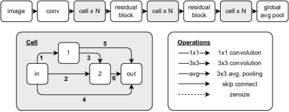
(Figure adapted from (Dong & Yang, 2020))
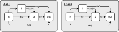
NAS-Bench-201 (Dong & Yang, 2020) is a cell-based architecture search space. Each cell has in total nodes and edges. The nodes in this search space correspond to the architecture’s feature maps and the edges represent the architectures operation, which are chosen from the operation set (see Figure 1). This search space contains in total architectures, from which only are unique, since the operations and can cause isomorphic cells (see Figure 8, appendix), where the latter operation stands for dropping the edge. Each architecture is trained on three different image datasets for epochs: CIFAR-10 (Krizhevsky, 2009), CIFAR-100 (Krizhevsky, 2009) and ImageNet16-120 (Chrabaszcz et al., 2017). For our evaluations, we consider all unique architectures in the search space and test splits of the corresponding datasets. Hence, we evaluate pretrained networks in total. In the following, we describe which evaluations we collect.
3.2 Robustness to Adversarial Attacks
We start by collecting evaluations on different adversarial attacks, namely FGSM, PGD, APGD, and Square Attack. Following, we describe each attack and the collection of their results in more detail.
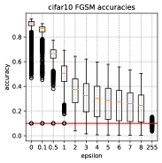
FGSM FGSM (Goodfellow et al., 2015) finds adversarial examples via
| (1) |
where is the adversarial example, is the input image, the corresponding label, the magnitude of the perturbation, and the network parameters. is the loss function used to train the attacked network. In the case of architectures trained for NAS-Bench-201, this is cross entropy (CE). Since attacks via FGSM can be evaluated fairly efficiently, we evaluate all architectures for , so for a total of times for each architecture. We use Foolbox (Rauber et al., 2017) to perform the attacks, and collect (a) accuracy, (b) average prediction confidences, as well as (c) confusion matrices for each network and combination.
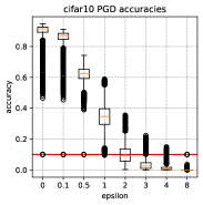
PGD While FGSM perturbs the image in a single step of size , PGD (Kurakin et al., 2017) iteratively perturbs the image via
| (2) |
where is the least likely predicted class of the network, and is a function clipping to range . Due to its iterative nature, PGD is more efficient in finding adversarial examples, but requires more computation time. Therefore, we find it sufficient to evaluate PGD for , so for a total of times for each architecture. As for FGSM, we use Foolbox (Rauber et al., 2017) to perform the attacks using their PGD implementation and keep the default settings, which are for attack iterations. We collect (a) accuracy, (b) average prediction confidences, and (c) confusion matrices for each network and combination.
APGD AutoAttack (Croce & Hein, 2020) offers an adaptive version of PGD that reduces its step size over time without the need for hyperparameters. We perform this attack using the implementation provided by (Croce & Hein, 2020) on CE and choose . We kept the default number of attack iterations that is . We collect (a) accuracy, (b) average prediction confidences, and (c) confusion matrices for each network and combination.
Square Attack In contrast to the before-mentioned attacks, Square Attack is a blackbox attack that has no access to the networks’ gradients. It solves the following optimization problem using random search:
| (3) |
where are the network predictions for class given an image. We perform this attack using the implementation provided by (Croce & Hein, 2020) and choose . We kept the default number of search iterations at . We collect (a) accuracy, (b) average prediction confidences, and (c) confusion matrices for each network and combination.
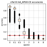
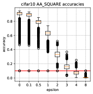
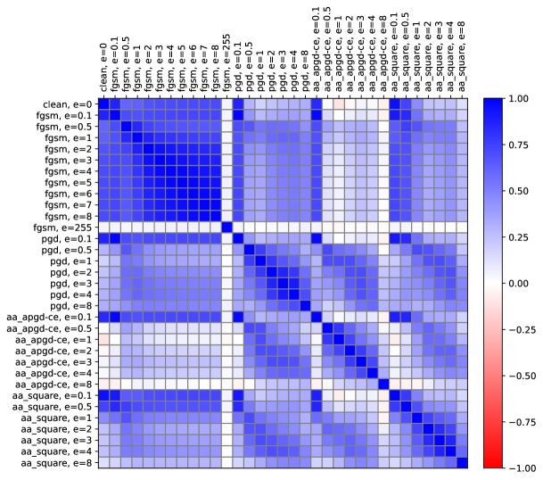
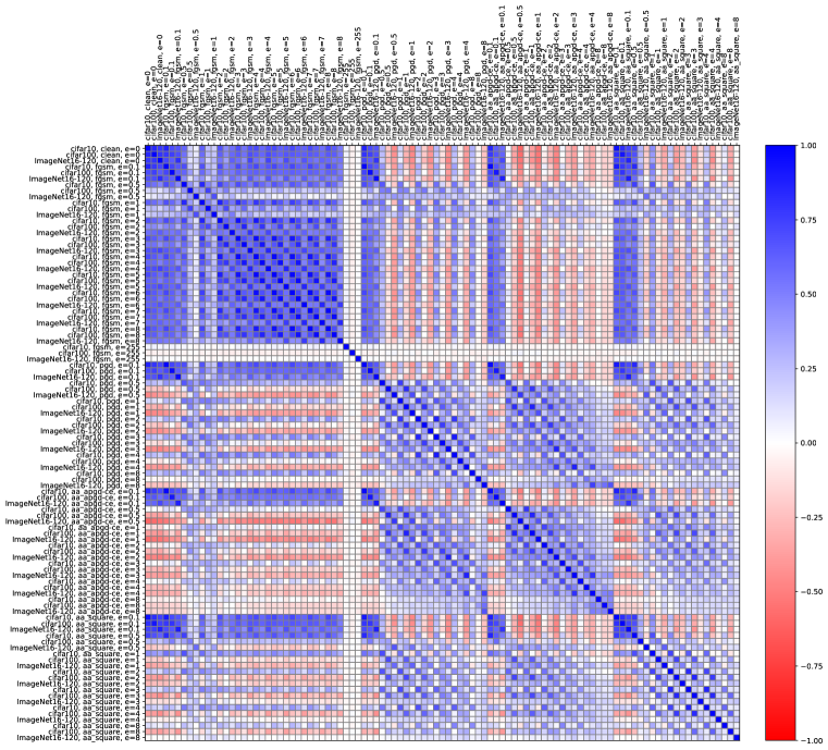
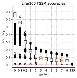
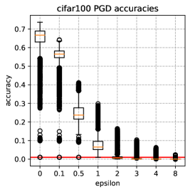
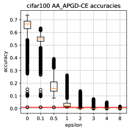
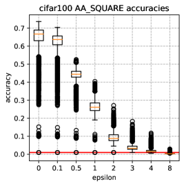
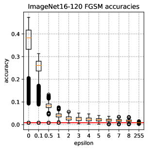
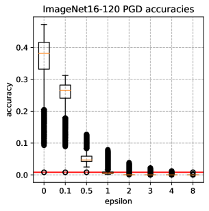
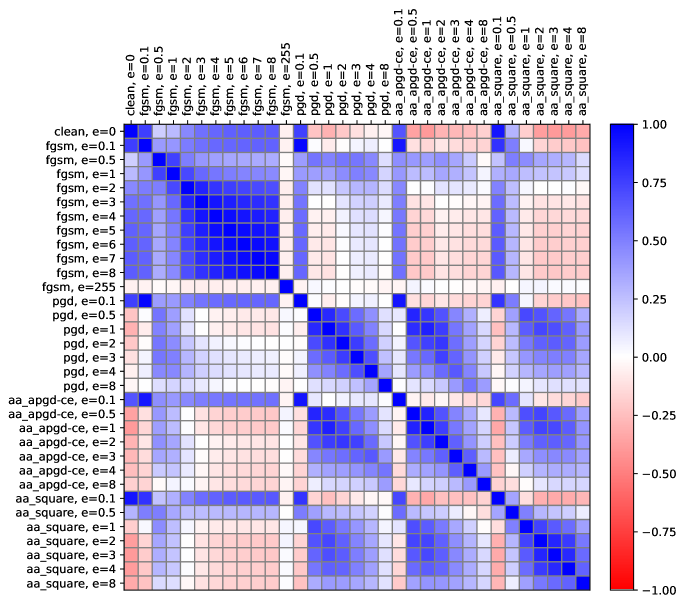
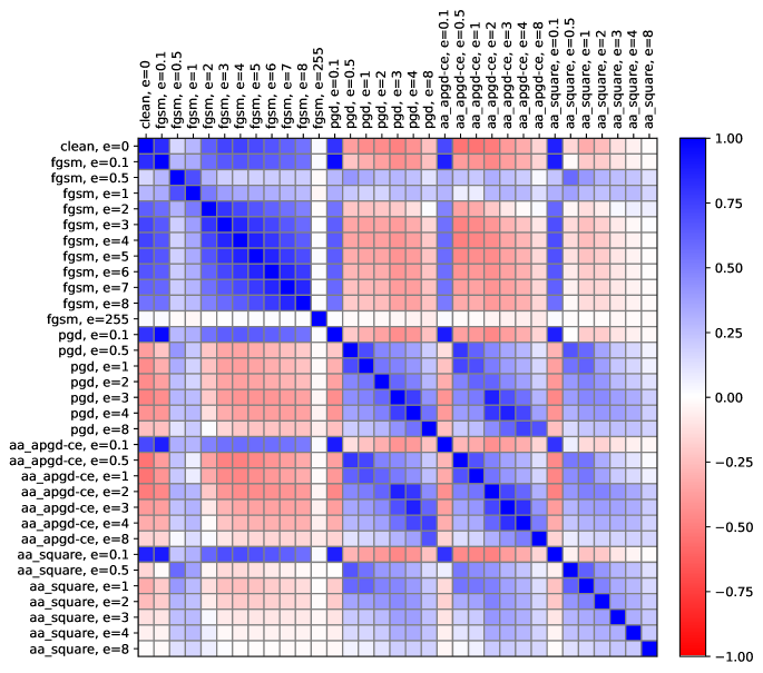
Summary Figure 2 shows aggregated evaluation results on the before-mentioned attacks on CIFAR-10 w.r.t. accuracy. Growing gaps between mean and max accuracies indicate that the architecture has an impact on robust performances. Figure 3 depicts the correlation of ranking all architectures based on different attack scenarios. While there is larger correlation within the same adversarial attack and different values of , there seem to be architectural distinctions for susceptibility to different attacks.


3.3 Robustness to Common Corruptions
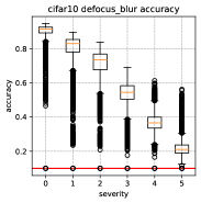
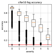
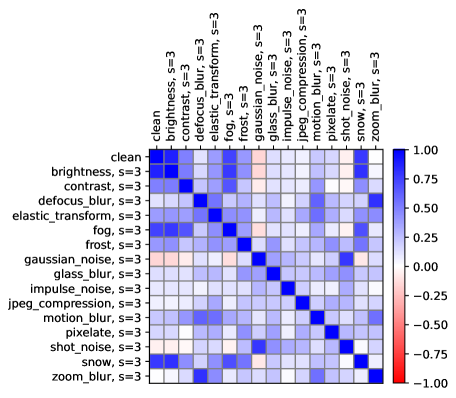
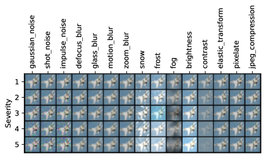
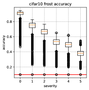
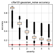
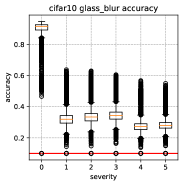
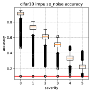
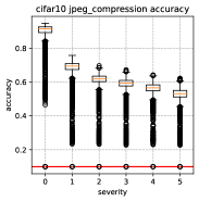
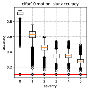
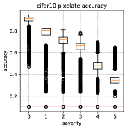
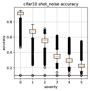
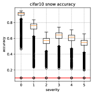
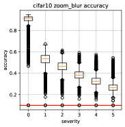
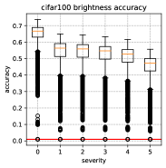
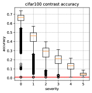
To evaluate all unique NAS-Bench-201 Dong & Yang (2020) architectures on common corruptions, we evaluate them on the benchmark data provided by (Hendrycks & Dietterich, 2019). Two datasets are available: CIFAR10-C, which is a corrupted version of CIFAR-10 and CIFAR-100-C, which is a corrupted version of CIFAR-100. Both datasets are perturbed with a total of corruptions at severity levels (see Figure 18 in the Appendix for an example). The training procedure of NAS-Bench-201 only augments the training data with random flipping and random cropping. Hence, no influence should be expected of the training augmentation pipeline on the performance of the networks to those corruptions. We evaluate each of the datasets individually for each network and collect (a) accuracy, (b) average prediction confidences, and (c) confusion matrices.
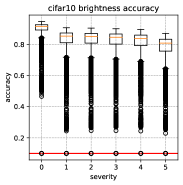
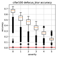
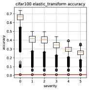
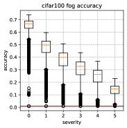
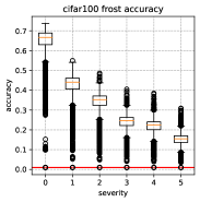
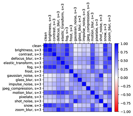
Summary Figure 4 depicts mean accuracies for different corruptions at increasing severity levels. Similar to Figure 2, a growing gap between mean and max accuracies for most of the corruptions can be observed, which indicates towards architectural influences on robustness to common corruptions. Figure 5 depicts the ranking correlation for all architectures between clean and corrupted accuracies. Ranking architectures based on accuracy on different kinds of corruption is mostly uncorrelated. This indicates a high diversity of sensitivity to different kinds of corruption based on architectural design.
4 Use Cases
4.1 Training-Free Measurements for Robustness
Recently, a new research focus in differentiable NAS shifted towards finding not only high-scoring architectures but also finding adversarially robust architectures against several adversarial attacks (Hosseini et al., 2021; Mok et al., 2021) using training characteristics of neural networks. On the one hand, (Hosseini et al., 2021) uses Jacobian-based differentiable metrics to measure robustness. On the other hand, (Mok et al., 2021) improves the search for robust architectures by including the smoothness of the loss landscape of a neural network. In this section, we evaluate these training-free gradient-based measurements with our dataset.
Background: Jacobian To improve the robustness of neural architectures, (Hoffman et al., 2019) introduced an efficient Jacobian regularization method with the goal to minimize the network’s output change in case of perturbed input data, by minimizing the Frobenius norm of the network’s Jacobian matrix, . The Frobenius norm is defined as Let be a neural network with weights denoted by and let be the input data and be the output score. Let be a perturbed input, with being a perturbation vector. The output of the neural network shifts then to . The input-output Jacobian matrix can be used as a measurement for the networks stability against input perturbations (Hoffman et al., 2019):
| (4) |
according to Taylor-expansion. From Equation 4, we can directly see that the larger the Jacobian components, the larger is the output change and thus the more unstable is the neural network against perturbed input data. In order to increase the stability of the network, (Hoffman et al., 2019) proposes to decrease the Jacobian components by minimizing the square of the Frobenius norm of the Jacobian. Following (Hosseini et al., 2021), we use the efficient algorithm presented in (Hoffman et al., 2019) to compute the Frobenius norm based on random projection for each neural network in the NAS-Bench-201 (Dong & Yang, 2020) benchmark.
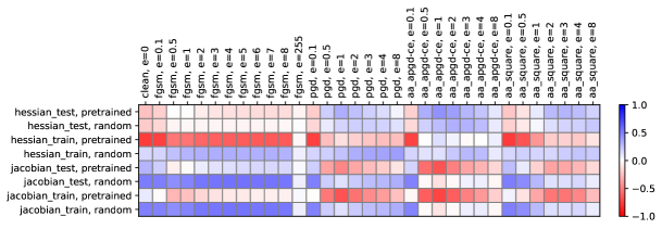
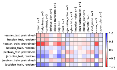
Benchmarking Results: Jacobian The smaller the Frobenius norm of the Jacobian of a network, the more robust the network is supposed to be. Our dataset allows for a direct evaluation of this statement on all unique architectures. We use mini-batches of size of the training as well as test dataset for both randomly initialized and pretrained networks and compute the mean Frobenius norm. The results in terms of ranking correlation to adversarial robustness is shown in Figure 6 (top), and in terms of ranking correlation to robustness towards common corruptions in Figure 6 (bottom). We can observe that the Jacobian-based measurement correlates well with rankings after attacks by FGSM and smaller values for other attacks. However, this is not true anymore when increases, especially in the case of APGD.
Background: Hessian Zhao et al. (2020) investigate the loss landscape of a regular neural network and robust neural network against adversarial attacks. Let denote the standard classification loss of a neural network for clean input data and be the adversarial loss with perturbed input data . Zhao et al. (2020) provide theoretical justification that the latter adversarial loss is highly correlated with the largest eigenvalue of the input Hessian matrix of the clean input data , denoted by . Therefore the eigenspectrum of the Hessian matrix of the regular network can be used for quantifying the robustness: large Hessian spectrum implies a sharp minimum resulting in a more vulnerable neural network against adversarial attacks. Whereas in the case of a neural network with small Hessian spectrum, implying a flat minimum, more perturbation on the input is needed to leave the minimum. We make use of (Chatzimichailidis et al., 2019) to compute the largest eigenvalue for each neural network in the NAS-Bench-201 (Dong & Yang, 2020) benchmark.
Benchmarking Results: Hessian For this measurement, we calculate the largest eigenvalues of all unique architectures using the Hessian approximation in (Chatzimichailidis et al., 2019). We use mini-batches of size of the training as well as test dataset for both randomly initialized and pretrained networks and compute the mean largest eigenvalue. These results are also shown in Figure 6. We can observe that the Hessian-based measurement behaves similarly to the Jacobian-based measurement.
| Test Accuracy () | |||||||
| Method | Clean | FGSM | PDG | APGD | Squares | Clean | |
| CIFAR-10 | CF-10-C | ||||||
| Optimum | |||||||
| Clean | BANANAS (White et al., 2021a) | ||||||
| Local Search (White et al., 2021b) | |||||||
| Random Search (Li & Talwalkar, 2019) | |||||||
| Regularized Evolution (Real et al., 2019) | |||||||
| FGSM | BANANAS (White et al., 2021a) | ||||||
| Local Search (White et al., 2021b) | |||||||
| Random Search (Li & Talwalkar, 2019) | |||||||
| Regularized Evolution (Real et al., 2019) | |||||||
4.2 NAS on Robustness
In this section, we perform different state-of-the-art NAS algorithms on the clean accuracy and the FGSM () robust accuracy in the NAS-Bench-201 (Dong & Yang, 2020) search space, and evaluate the best found architectures on all provided introduced adversarial attacks. We apply random search (Li & Talwalkar, 2019), local search (White et al., 2021b), regularized evolution (Real et al., 2019) and BANANAS (White et al., 2021a) with a maximal query amount of . The results are shown in Table 1. Although clean accuracy is reduced, the overall robustness to all adversarial attacks improves when the search is performed on FGSM () accuracy. Local Search achieves the best performance, which indicates that localized changes to an architecture design seem to be able to improve network robustness.
4.3 Analyzing the Effect of Architecture Design on Robustness
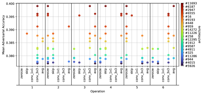
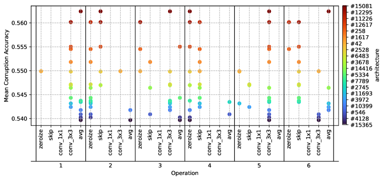
In Figure 7, we show the top-20 performing architectures (color-coded, one operation for each edge) with exactly times convolutions and no convolutions (hence, the same parameter count), according to the mean adversarial accuracy over all attacks as described in subsection 3.2 on CIFAR-10. It is interesting to see that there are no convolutions on edges and , and additionally no dropping (operation zeroize) or skipping (operation skip-connect) of edge . In the case of edge , it seems that a single convolutional layer connecting input and output of the cell increases sensitivity of the network. Hence, most of the top-20 robust architectures stack convolutions (via edge , followed by either edge or ), from which we hypothesize that stacking convolution operations might improve robustness when designing architectures. At the same time, skipping input to output via edge seems not to affect robustness negatively, as long as the input feature map is combined with stacked convolutions. Further analyses can be found in Appendix B. We find that optimizing architecture design can have a substantial impact on the robustness of a network. In this setting, where networks have the same parameter count, we can see a large range of mean adversarial accuracies showing the potential of doubling the robustness of a network by carefully crafting its topology. Important to note here is that this is a first observation, which can be made by using our provided dataset. This observation functions as a motivation for how this dataset can be used to analyze robustness in combination with architecture design.
5 Conclusion
We introduce a dataset for neural architecture design and robustness to provide the research community with more resources for analyzing what constitutes robust networks. We have evaluated all unique architectures from the commonly used NAS-Bench-201 benchmark against several adversarial attacks and image dataset corruptions. With this full evaluation at hand, we presented three use cases for this dataset: First, the correlation between the robustness of the architectures and two differentiable architecture measurements. We showed that these measurements are a good first approach for the architecture’s robustness, but have to be taken with caution when the perturbation increases. Second, neural architecture search directly on the robust accuracies, which indeed finds more robust architectures for different adversarial attacks. And last, an initial analysis of architectural design, where we showed that it is possible to improve robustness of networks with the same number of parameters by carefully designing their topology.
Limitations and Broader Impact We show that carefully crafting the architectural design can lead to substantial impact on the architecture’s robustness. This paper aims to promote and streamline research on how the architecture design affects model robustness. It does so by evaluating pretrained architectures and is thus complementary to any work focusing on the analysis of different, potentially adversarial, training protocols.
Reproducibility
In order to ensure reproducibility, we build our dataset on architectures from a common NAS-Benchmark, which is described in the main paper in subsection 3.1. In addition, all hyperparameters for reproducing the robustness results are given in subsection 3.2. Lastly, a complete description of the dataset itself is provided in the appendix, Appendix A.
References
- Andriushchenko et al. (2020) Maksym Andriushchenko, Francesco Croce, Nicolas Flammarion, and Matthias Hein. Square attack: a query-efficient black-box adversarial attack via random search. In European Conference on Computer Vision, pp. 484–501. Springer, 2020.
- Bender et al. (2018) Gabriel Bender, Pieter-Jan Kindermans, Barret Zoph, Vijay Vasudevan, and Quoc V. Le. Understanding and simplifying one-shot architecture search. In ICML, 2018.
- Bergstra & Bengio (2012) James Bergstra and Yoshua Bengio. Random search for hyper-parameter optimization. Journal of Machine Learning Research, 13(10):281–305, 2012.
- Cai et al. (2019) Han Cai, Ligeng Zhu, and Song Han. Proxylessnas: Direct neural architecture search on target task and hardware. In ICLR, 2019.
- Carlini et al. (2019) Nicholas Carlini, Anish Athalye, Nicolas Papernot, Wieland Brendel, Jonas Rauber, Dimitris Tsipras, Ian J. Goodfellow, Aleksander Madry, and Alexey Kurakin. On evaluating adversarial robustness. CoRR, abs/1902.06705, 2019. URL http://arxiv.org/abs/1902.06705.
- Chatzimichailidis et al. (2019) Avraam Chatzimichailidis, Janis Keuper, Franz-Josef Pfreundt, and Nicolas R. Gauger. Gradvis: Visualization and second order analysis of optimization surfaces during the training of deep neural networks. In Workshop on Machine Learning in High Performance Computing Environments, MLHPC@SC, 2019.
- Chrabaszcz et al. (2017) Patryk Chrabaszcz, Ilya Loshchilov, and Frank Hutter. A downsampled variant of imagenet as an alternative to the CIFAR datasets. CoRR, abs/1707.08819, 2017.
- Croce & Hein (2020) Francesco Croce and Matthias Hein. Reliable evaluation of adversarial robustness with an ensemble of diverse parameter-free attacks. In International conference on machine learning, pp. 2206–2216. PMLR, 2020.
- Croce et al. (2021) Francesco Croce, Maksym Andriushchenko, Vikash Sehwag, Edoardo Debenedetti, Nicolas Flammarion, Mung Chiang, Prateek Mittal, and Matthias Hein. Robustbench: a standardized adversarial robustness benchmark. In Joaquin Vanschoren and Sai-Kit Yeung (eds.), NeurIPS Datasets and Benchmarks, 2021.
- Deng et al. (2009) Jia Deng, Wei Dong, Richard Socher, Li-Jia Li, Kai Li, and Li Fei-Fei. ImageNet: A large-scale hierarchical image database. In CVPR, 2009.
- Devaguptapu et al. (2021) Chaitanya Devaguptapu, Devansh Agarwal, Gaurav Mittal, Pulkit Gopalani, and Vineeth N. Balasubramanian. On adversarial robustness: A neural architecture search perspective. In ICCVW, 2021.
- Dodge & Karam (2017) Samuel F. Dodge and Lina J. Karam. A study and comparison of human and deep learning recognition performance under visual distortions. CoRR, abs/1705.02498, 2017. URL http://arxiv.org/abs/1705.02498.
- Dong et al. (2020a) Minjing Dong, Yanxi Li, Yunhe Wang, and Chang Xu. Adversarially robust neural architectures. CoRR, abs/2009.00902, 2020a.
- Dong & Yang (2019) Xuanyi Dong and Yi Yang. Searching for a robust neural architecture in four GPU hours. In CVPR, 2019.
- Dong & Yang (2020) Xuanyi Dong and Yi Yang. Nas-bench-201: Extending the scope of reproducible neural architecture search. In ICLR, 2020.
- Dong et al. (2020b) Yinpeng Dong, Qi-An Fu, Xiao Yang, Tianyu Pang, Hang Su, Zihao Xiao, and Jun Zhu. Benchmarking adversarial robustness on image classification. In 2020 IEEE/CVF Conference on Computer Vision and Pattern Recognition (CVPR), pp. 318–328, 2020b. doi: 10.1109/CVPR42600.2020.00040.
- Duan et al. (2021) Yawen Duan, Xin Chen, Hang Xu, Zewei Chen, Xiaodan Liang, Tong Zhang, and Zhenguo Li. Transnas-bench-101: Improving transferability and generalizability of cross-task neural architecture search. In CVPR, 2021.
- Goodfellow et al. (2015) Ian J. Goodfellow, Jonathon Shlens, and Christian Szegedy. Explaining and harnessing adversarial examples. In Yoshua Bengio and Yann LeCun (eds.), 3rd International Conference on Learning Representations, ICLR 2015, San Diego, CA, USA, May 7-9, 2015, Conference Track Proceedings, 2015. URL http://arxiv.org/abs/1412.6572.
- Guo et al. (2020) Minghao Guo, Yuzhe Yang, Rui Xu, Ziwei Liu, and Dahua Lin. When NAS meets robustness: In search of robust architectures against adversarial attacks. In CVPR, 2020.
- He et al. (2015) Kaiming He, Xiangyu Zhang, Shaoqing Ren, and Jian Sun. Delving deep into rectifiers: Surpassing human-level performance on imagenet classification. In 2015 IEEE International Conference on Computer Vision (ICCV), pp. 1026–1034, 2015. doi: 10.1109/ICCV.2015.123.
- Hendrycks & Dietterich (2019) Dan Hendrycks and Thomas Dietterich. Benchmarking neural network robustness to common corruptions and perturbations. Proceedings of the International Conference on Learning Representations, 2019.
- Hoffman et al. (2019) Judy Hoffman, Daniel A. Roberts, and Sho Yaida. Robust learning with jacobian regularization. CoRR, abs/1908.02729, 2019.
- Hosseini et al. (2021) Ramtin Hosseini, Xingyi Yang, and Pengtao Xie. DSRNA: differentiable search of robust neural architectures. In CVPR, 2021.
- Kandasamy et al. (2018) Kirthevasan Kandasamy, Willie Neiswanger, Jeff Schneider, Barnabás Póczos, and Eric P. Xing. Neural architecture search with bayesian optimisation and optimal transport. In NIPS, 2018.
- Krizhevsky (2009) Alex Krizhevsky. Learning multiple layers of features from tiny images. In Technical report, 2009.
- Krizhevsky et al. (2012) Alex Krizhevsky, Ilya Sutskever, and Geoffrey E. Hinton. Imagenet classification with deep convolutional neural networks. In NIPS, 2012.
- Kurakin et al. (2017) Alexey Kurakin, Ian Goodfellow, and Samy Bengio. Adversarial machine learning at scale, 2017.
- Li & Talwalkar (2019) Liam Li and Ameet Talwalkar. Random search and reproducibility for neural architecture search. In UAI, 2019.
- Li et al. (2018) Yujia Li, Oriol Vinyals, Chris Dyer, Razvan Pascanu, and Peter W. Battaglia. Learning deep generative models of graphs. CoRR, abs/1803.03324, 2018.
- Ling et al. (2019) Xiang Ling, Shouling Ji, Jiaxu Zou, Jiannan Wang, Chunming Wu, Bo Li, and Ting Wang. Deepsec: A uniform platform for security analysis of deep learning model. In 2019 IEEE Symposium on Security and Privacy (SP), pp. 673–690, 2019. doi: 10.1109/SP.2019.00023.
- Liu et al. (2019) Hanxiao Liu, Karen Simonyan, and Yiming Yang. DARTS: differentiable architecture search. In ICLR, 2019.
- Lukasik et al. (2021) Jovita Lukasik, David Friede, Arber Zela, Frank Hutter, and Margret Keuper. Smooth variational graph embeddings for efficient neural architecture search. In International Joint Conference on Neural Networks, IJCNN 2021, Shenzhen, China, July 18-22, 2021, pp. 1–8. IEEE, 2021.
- Lukasik et al. (2022) Jovita Lukasik, Steffen Jung, and Margret Keuper. Learning where to look - generative NAS is surprisingly efficient. In Computer Vision - ECCV 2022 - 17th European Conference, Tel Aviv, Israel, October 23-27, 2022, Proceedings, Part XXIII, volume 13683 of Lecture Notes in Computer Science, pp. 257–273. Springer, 2022.
- Mok et al. (2021) Jisoo Mok, Byunggook Na, Hyeokjun Choe, and Sungroh Yoon. Advrush: Searching for adversarially robust neural architectures. In ICCV, 2021.
- Pang et al. (2021) Tianyu Pang, Xiao Yang, Yinpeng Dong, Hang Su, and Jun Zhu. Bag of tricks for adversarial training. In 9th International Conference on Learning Representations, ICLR 2021, Virtual Event, Austria, May 3-7, 2021. OpenReview.net, 2021. URL https://openreview.net/forum?id=Xb8xvrtB8Ce.
- Pham et al. (2018) Hieu Pham, Melody Y. Guan, Barret Zoph, Quoc V. Le, and Jeff Dean. Efficient neural architecture search via parameter sharing. In ICML, 2018.
- Rauber et al. (2017) Jonas Rauber, Wieland Brendel, and Matthias Bethge. Foolbox: A python toolbox to benchmark the robustness of machine learning models. In Reliable Machine Learning in the Wild Workshop, 34th International Conference on Machine Learning, 2017. URL http://arxiv.org/abs/1707.04131.
- Real et al. (2017) Esteban Real, Sherry Moore, Andrew Selle, Saurabh Saxena, Yutaka Leon Suematsu, Jie Tan, Quoc V. Le, and Alexey Kurakin. Large-scale evolution of image classifiers. In ICML, 2017.
- Real et al. (2019) Esteban Real, Alok Aggarwal, Yanping Huang, and Quoc V. Le. Regularized evolution for image classifier architecture search. In AAAI, 2019.
- Rezaei et al. (2021) Seyed Saeed Changiz Rezaei, Fred X. Han, Di Niu, Mohammad Salameh, Keith G. Mills, Shuo Lian, Wei Lu, and Shangling Jui. Generative adversarial neural architecture search. In Proceedings of the Thirtieth International Joint Conference on Artificial Intelligence, IJCAI 2021, Virtual Event / Montreal, Canada, 19-27 August 2021, pp. 2227–2234. ijcai.org, 2021.
- Ru et al. (2021) Binxin Ru, Xingchen Wan, Xiaowen Dong, and Michael Osborne. Interpretable neural architecture search via bayesian optimisation with weisfeiler-lehman kernels. In ICLR, 2021.
- Su et al. (2018) Dong Su, Huan Zhang, Hongge Chen, Jinfeng Yi, Pin-Yu Chen, and Yupeng Gao. Is robustness the cost of accuracy? - a comprehensive study on the robustness of 18 deep image classification models. In ECCV, 2018.
- Szegedy et al. (2014) Christian Szegedy, Wojciech Zaremba, Ilya Sutskever, Joan Bruna, Dumitru Erhan, Ian Goodfellow, and Rob Fergus. Intriguing properties of neural networks. In International Conference on Learning Representations, 2014. URL http://arxiv.org/abs/1312.6199.
- Tang et al. (2021) Shiyu Tang, Ruihao Gong, Yan Wang, Aishan Liu, Jiakai Wang, Xinyun Chen, Fengwei Yu, Xianglong Liu, Dawn Xiaodong Song, Alan Loddon Yuille, Philip H. S. Torr, and Dacheng Tao. Robustart: Benchmarking robustness on architecture design and training techniques. ArXiv, abs/2109.05211, 2021.
- White et al. (2021a) Colin White, Willie Neiswanger, and Yash Savani. Bananas: Bayesian optimization with neural architectures for neural architecture search. In AAAI, 2021a.
- White et al. (2021b) Colin White, Sam Nolen, and Yash Savani. Exploring the loss landscape in neural architecture search. In UAI, 2021b.
- Xie et al. (2019a) Cihang Xie, Yuxin Wu, Laurens van der Maaten, Alan Loddon Yuille, and Kaiming He. Feature denoising for improving adversarial robustness. 2019 IEEE/CVF Conference on Computer Vision and Pattern Recognition (CVPR), pp. 501–509, 2019a.
- Xie et al. (2020) Cihang Xie, Mingxing Tan, Boqing Gong, Alan Loddon Yuille, and Quoc V. Le. Smooth adversarial training. ArXiv, abs/2006.14536, 2020.
- Xie et al. (2019b) Sirui Xie, Hehui Zheng, Chunxiao Liu, and Liang Lin. SNAS: stochastic neural architecture search. In ICLR, 2019b.
- Xu et al. (2020) Yuhui Xu, Lingxi Xie, Xiaopeng Zhang, Xin Chen, Guo-Jun Qi, Qi Tian, and Hongkai Xiong. PC-DARTS: partial channel connections for memory-efficient architecture search. In ICLR, 2020.
- Ying et al. (2019) Chris Ying, Aaron Klein, Eric Christiansen, Esteban Real, Kevin Murphy, and Frank Hutter. Nas-bench-101: Towards reproducible neural architecture search. In ICML, 2019.
- Zela et al. (2020) Arber Zela, Thomas Elsken, Tonmoy Saikia, Yassine Marrakchi, Thomas Brox, and Frank Hutter. Understanding and robustifying differentiable architecture search. In ICLR, 2020.
- Zhao et al. (2020) Pu Zhao, Pin-Yu Chen, Payel Das, Karthikeyan Natesan Ramamurthy, and Xue Lin. Bridging mode connectivity in loss landscapes and adversarial robustness. In ICLR, 2020.
- Zoph & Le (2017) Barret Zoph and Quoc V. Le. Neural architecture search with reinforcement learning. In ICLR, 2017.
Appendix A Dataset
A.1 NAS-Bench-201
We base our evaluations on the NAS-Bench-201 (Dong & Yang, 2020) search space. It is a cell-based architecture search space. Each cell has in total nodes and edges. The nodes in this search space correspond to the architecture’s feature maps and the edges represent the architectures operation, which are chosen from the operation set (see Figure 1). This search space contains in total architectures, from which only are unique, since the operations and can cause isomorphic cells (see Figure 8), where the latter operation stands for dropping the edge. Each architecture is trained on three different image datasets for epochs: CIFAR-10 (Krizhevsky, 2009), CIFAR-100 (Krizhevsky, 2009) and ImageNet16-120 (Chrabaszcz et al., 2017). For our evaluations, we consider all unique architectures in the search space and test splits of the corresponding datasets. Hence, we evaluate pretrained networks in total.
A.2 Dataset Gathering
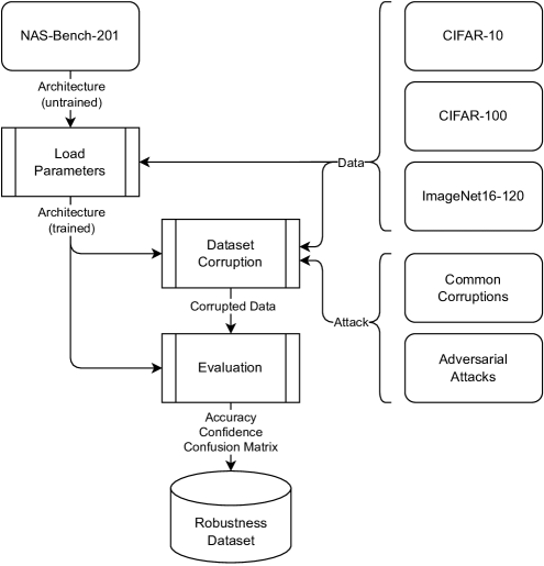
We collect evaluations for our dataset for different corruptions and adversarial attacks (as discussed in subsection 3.2 and subsection 3.3) following algorithm 1. This process is also depicted in Figure 9. Hyperparameter settings for adversarial attacks are listed in Table 2. Due to the heavy load of running all these evaluations, they are performed on several clusters. These clusters are comprised of either (i) compute nodes with Nvidia A100 GPUs, 512 GB RAM, and Intel Xeon IceLake-SP processors, (ii) compute nodes with NVIDIA Quadro RTX 8000 GPUs, 1024 GB RAM, and AMD EPYC 7502P processors, (iii) NVIDIA Tesla A100 GPUs, 2048 GB RAM, Intel Xeon Platinum 8360Y processors, and (iv) NVIDIA Tesla A40 GPUs, 2048 GB RAM, Intel Xeon Platinum 8360Y processors.
| Attack | Hyperparameters |
|---|---|
| FGSM | |
| PGD | |
| attack iterations | |
| APGD | |
| attack iterations | |
| Square | |
| search iterations |
A.3 Dataset Structure, Distribution, and License
Files are provided in json format to ensure platform-independence and to reduce the dependency on external libraries (e.g. Python has built-in json-support).
We will publish code that accompanies our dataset on GitHub. The dataset itself will be linked from GitHub and is hosted on an institutional cloud service. This ensures longtime availability and the possibility to version the dataset. Dataset and code will be published at the notification date under GNU GPLv3.
A.4 Structure
The dataset consists of folders, one for each dataset evaluated (cifar10, cifar100, ImageNet16-120). Each folder contains one json file for each combination of key and measurement. Keys refer to the sort of attack or corruption used (Table 3 lists all keys). Measurements refer to the collected evaluation type (accuracy, confidence, cm). Clean and adversarial evaluations are performed on all datasets, while common corruptions are evaluated on cifar10 and cifar100. Additionally, the dataset contains one metadata file (meta.json).
| Clean | Adversarial | Common Corruptions |
|---|---|---|
| clean | aa_apgd-ce | brightness |
| aa_square | contrast | |
| fgsm | defocus_blur | |
| pgd | elastic_transform | |
| fog | ||
| frost | ||
| gaussian_noise | ||
| glass_blur | ||
| impulse_noise | ||
| jpeg_compression | ||
| motion_blur | ||
| pixelate | ||
| shot_noise | ||
| snow | ||
| zoom_blur |
Metadata
The meta.json file contains information about each architecture in NAS-Bench-201. This includes, for each architecture identifier, the corresponding string defining the network design (as per (Dong & Yang, 2020)) as well as the identifier of the corresponding non-isomorphic architecture from (Dong & Yang, 2020) that we evaluated. The file also contains all values that we evaluated for each adversarial attack. An excerpt of this file is shown in Figure 10.
Files
All files are named according to "{key}_{measurement}.json". Hence, the path to all clean accuracies on cifar10 is "./cifar10/clean_accuracy.json". An excerpt of this file is shown in Figure 11. Each file contains nested dictionaries stating the dataset, evaluation key and measurement type. For evaluations with multiple measurements, e.g. in the case of adversarial attacks for multiple values, the results are concatenated into a list. Files and their possible contents are described in Table 4.
| File | Description |
|---|---|
| clean_accuracy | one accuracy value for each evaluated network |
| clean_confidence | one confidence matrix for each evaluated network and collection scheme |
| clean_cm | one confusion matrix for each evaluated network |
| {attack}_accuracy | list of accuracies, where each element corresponds to the respective value |
| {attack}_confidence | list of confidence matrices, where each element corresponds to the respective value |
| {attack}_cm | list of confusion matrices, where each element corresponds to the respective value |
| {corruption}_accuracy | list of accuracies, where each element corresponds to the respective corruption severity |
| {corruption}_confidence | list of confidence matrices, where each element corresponds to the respective corruption severity |
| {corruption}_cm | list of confusion matrices, where each element corresponds to the respective corruption severity |
We showed some analysis and possible use-cases on accuracies in the main paper. In the following, we elaborate on and show confidence and confusion matrix (cm) measurements.
A.5 Confidence
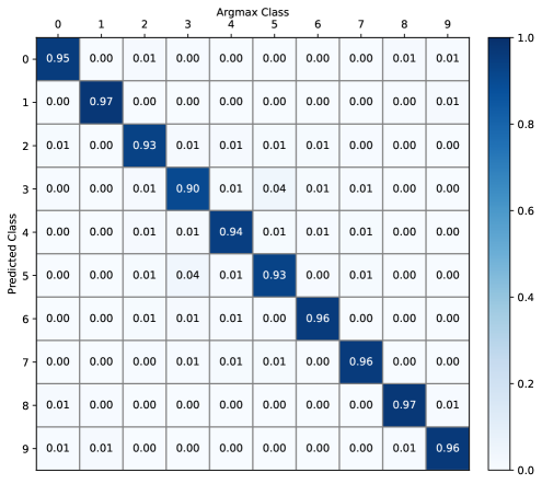
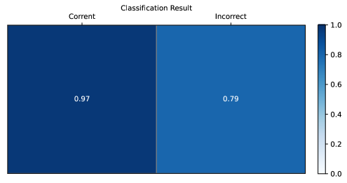
We collect the mean confidence after softmax for each network over the whole (attacked) test dataset evaluated. We used schemes to collect confidences (see Figure 13). First, confidences for each class are given by true labels (called label). In case of cifar10, this results in a confidence matrix, for cifar100 a confidence matrix, and ImageNet16-120 a confidence matrix. Second, confidences for each class are given by the class predicted by the network (called argmax). This again results in matrices of sizes as mentioned. Third, confidences for correctly classified images as well as confidences for incorrectly classified images (called prediction). For all image datasets, this results in a vector with dimensions. Each result is saved as a list (or list of list), see Figure 12.
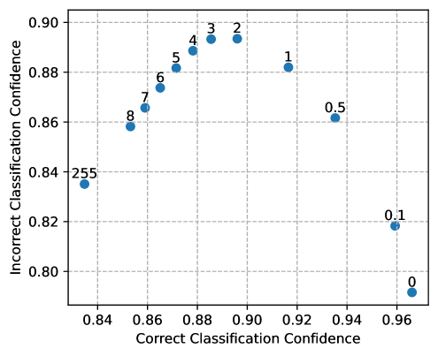
Figure 14 shows a progression of label confidence values for class label on cifar10 from clean to fgsm with increasing values of . Figure 15 shows how prediction confidences of correctly and incorrectly classified images correlate with increasing values of when attacked with fgsm.


A.6 Confusion Matrix
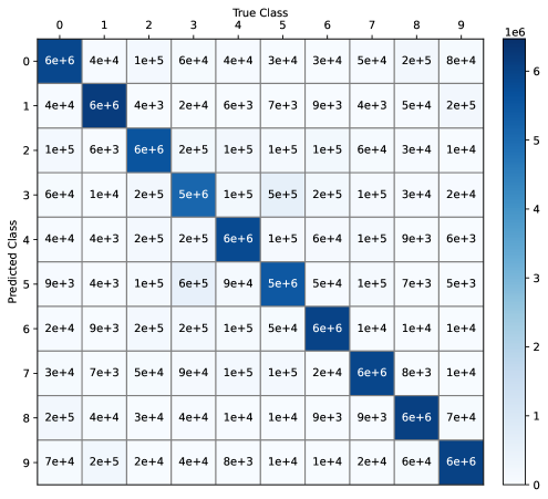
For each evaluated network, we collect the confusion matrix (key: cm) for the corresponding (attacked) test dataset. The result is a matrix in case of cifar10, a matrix in case of cifar100, and a matrix in case of ImageNet16-120. See Figure 16 for an example, where we summed up confusion matrices for all networks on cifar10.
A.7 Correlations between Image Datasets
In Figure 17 we show the correlation between all clean and adversarial accuracies over all datasets collected. This plot shows a positive correlation between the image datasets for the one-step FGSM attack, whereas for all other multi-step attacks, the correlation becomes close to zero or even negative.
A.8 Example image of corruptions in CIFAR-10-C
A.9 Main Paper Figures for other Image Datasets
A.9.1 CIFAR-100 Adversarial Attack Accuracies (Figure 2)
A.9.2 ImageNet16-120 Adversarial Attack Accuracies (Figure 2)
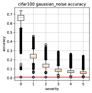
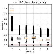
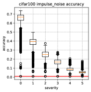
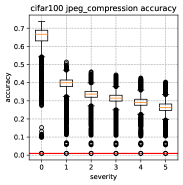
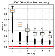
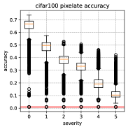
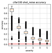
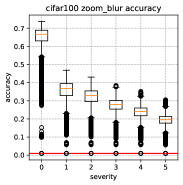
A.9.3 CIFAR-10-C Common Corruption Accuracies (Figure 4)


A.9.4 CIFAR-100-C Common Corruption Accuracies (Figure 4)

A.9.5 CIFAR-100 Adversarial Attack Correlations (Figure 3)
A.9.6 ImageNet16-120 Adversarial Attack Correlations (Figure 3)
A.9.7 CIFAR-100-C Common Corruption Correlations (Figure 5)
Appendix B Analysis
In this section, we first depict the best architectures in NAS-Bench-201 (Dong & Yang, 2020) in subsection B.1, then show the effect of parameter count on robustness and the magnitude of potential gains in robustness in a limited parameter count setting in subsection B.2, and lastly show the effect of single changes to the best performing architecture according to clean accuracy in subsection B.3.
B.1 Best Architectures
Figure 26 visualizes the best architectures in the NAS-Bench-201 (Dong & Yang, 2020) search space in terms of clean accuracy, mean adversarial accuracy, and mean common corruption accuracy on CIFAR-10 and their respective edit distances. The edit distance is defined by the number of changes, either node or edge, to change the graph to the target graph. In the case of NAS-Bench-201 architectures, an edit distance of means that exactly one operation differs between two architectures. So in order to modify the best performing architecture in terms of clean accuracy () into the best performing architecture according to mean corruption accuracy (), we need to exchange two (out of six) operations: (i) exchange operation from convolution to and (ii) exchange operation from convolution to convolution.
B.2 Cell Kernel Parameter Count
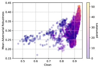
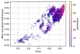
Figure 27 displays the mean adversarial robustness accuracies (left) and the mean corruption robustness accuracies (right) against the clean accuracy, color-coded by the number of cell kernel parameters. We count for each convolution and for each convolution contained in the cell, hence, their number ranges in . Since these are multipliers for the parameter count of the whole network, we coin these cell kernel parameters. Overall, we can see that the cell kernel parameter count matters in terms of robustness, hence, that networks with large parameter counts are more robust in general. We can also see that the number of cell kernel parameters are more essential for robustness against common corruptions, where the correlation between clean and corruption accuracy is more linear. Also in terms of adversarial robustness, there seems to be a large magnitude of possible improvements that can be gained by optimizing architecture design.
Limited Cell Parameter Count
To further investigate the magnitude of possible improvements via architectural design optimization, we look into the scenario of limited cell parameter count.
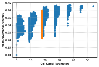
In Figure 28, we depict all unique architectures in NAS-Bench-201 by their mean adversarial robustness and cell kernel parameter count. Networks with parameter count ( instances in total) are highlighted in orange. As we can see, there is a large range of mean adversarial accuracies for the parameter count showing the potential of doubling the robustness of a network with the same parameter count by carefully crafting its topology. In Figure 29 we show the top-20 performing architectures (color-coded, one operation for each edge) in the mentioned scenario of a parameter count of , according to (top) mean adversarial and (bottom) mean corruption accuracy. It is interesting to see that in both cases, there are (almost) no convolutions on edges and , and additionally no dropping or skipping of edge . In the case of edge , it seems that a single convolution layer connecting input and output of the cell increases sensitivity of the network. Hence, most of the top-20 robust architectures stack convolutions (via edge , followed by either edge or ), from which we hypothesize that stacking convolutions operations might improve robustness when designing architectures. At the same time, skipping input to output via edge seems not to affect robustness negatively, as long as the input feature map is combined with stacked convolutions. Important to note here is that this is a first observation, which can be made by using our provided dataset. This observation functions as a motivation for how this dataset can be used to analyze robustness in combination with architecture design.

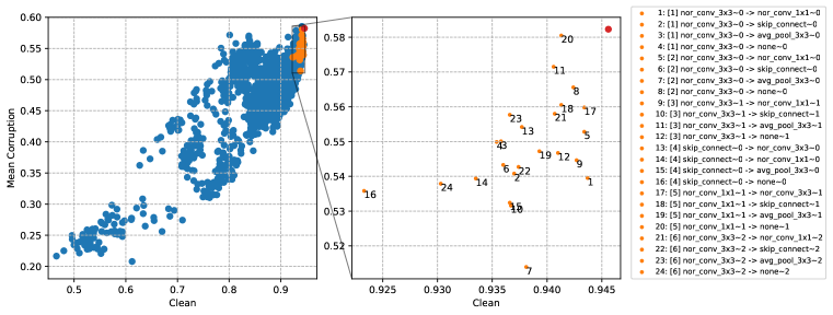
B.3 Gains and Losses by Single Changes
The fact that our dataset contains evaluations for all unique architectures in NAS-Bench-201 enables us to analyze the effect of small architectural changes. In Figure 30, we depict again all unique architectures by their clean and robust accuracies on CIFAR-10 (Krizhevsky, 2009). The red data point in both plots shows the best performing architecture in terms of clean accuracy (, see Figure 26), while the orange points are its neighboring architectures with edit distance . The operation changed for each point is shown in the legend. As we can see in the case of adversarial attacks, we can trade-off more robust accuracy for less clean accuracy by changing only one operation. While some changes seem obvious (adding more parameters as with and ), it is interesting to see that exchanging the convolution on edge with average pooling (and hence, reducing the amount of parameters) also improves adversarial robustness. In terms of robustness towards common corruptions, each architectural change leads to worse clean and robust accuracy in this case. Changing more than one operation is necessary to improve common corruption accuracy of this network (as we have seen in Figure 26).