Predicting Software Performance with Divide-and-Learn

Abstract.

Predicting the performance of highly configurable software systems is the foundation for performance testing and quality assurance. To that end, recent work has been relying on machine/deep learning to model software performance. However, a crucial yet unaddressed challenge is how to cater for the sparsity inherited from the configuration landscape: the influence of configuration options (features) and the distribution of data samples are highly sparse.

In this paper, we propose an approach based on the concept of “divide-and-learn”, dubbed DaL. The basic idea is that, to handle sample sparsity, we divide the samples from the configuration landscape into distant divisions, for each of which we build a regularized Deep Neural Network as the local model to deal with the feature sparsity. A newly given configuration would then be assigned to the right model of division for the final prediction.

Experiment results from eight real-world systems and five sets of training data reveal that, compared with the state-of-the-art approaches, DaL performs no worse than the best counterpart on 33 out of 40 cases (within which 26 cases are significantly better) with up to $1.94\times$ improvement on accuracy; requires fewer samples to reach the same/better accuracy; and producing acceptable training overhead. Practically, DaL also considerably improves different global models when using them as the underlying local models, which further strengthens its flexibility. To promote open science, all the data, code, and supplementary figures of this work can be accessed at our repository: https://github.com/ideas-labo/DaL.

1. Introduction

“What will be the implication on runtime if we deploy that configuration?”

The above is a question we often hear from our industrial partners. Indeed, software performance, such as latency, runtime, and energy consumption, is one of the most critical concerns of software systems that come with a daunting number of configuration options, e.g., x264 (a video encoder) allows one to adjust 16 options to influence its runtime. To satisfy the performance requirements, it is essential for software engineers to understand what performance can be obtained under a given configuration before the deployment. This not only enables better decisions on configuration tuning (Chen and Li, 2023) but also reduces the efforts of configuration testing (Ferme and Pautasso, 2017).

To achieve the above, one way is to directly profile the software system for all possible configurations when needed. This, however, is impractical, because (1) the number of possible configurations may be too high (Jamshidi and Casale, 2016; Chen and Li, 2021; Siegmund et al., 2015; Ha and Zhang, 2019a). For example, HIPA^cc (a compiler for image processing) has more than 10,000 possible configurations. (2) Even when such a number is small, the profiling of a single configuration can still be rather expensive (Jamshidi and Casale, 2016; Chen and Li, 2021): Wang et al. (Wang et al., 2013) report that it could take weeks of running time to benchmark and profile even a simple system. Therefore, an accurate performance model that can predict the expected performance of a newly given configuration is of high demand.

With the increasing complexity of modern software, the number of configurable options continues to expand and the interactions between options become more complicated, leading to significant difficulty in predicting the performance accurately (Siegmund et al., 2012a; Chen and Bahsoon, 2017). Recently, machine learning models have been becoming the promising method for this regression problem as they are capable of modeling the complex interplay between a large number of variables by observing patterns from data (Weber et al., 2021; Velez et al., 2021; Han et al., 2021; Siegmund et al., 2015; Shu et al., 2020; Siegmund et al., 2012b; Ha and Zhang, 2019a).

However, since machine learning modeling is data-driven, the characteristics and properties of the measured data for configurable software systems pose non-trivial challenges to the learning, primarily because it is known that the configuration landscapes of the systems do not follow a “smooth” shape (Jamshidi and Casale, 2016). For example, adjusting between different cache strategies can drastically influence the performance, but they are often represented as a single-digit change on the landscape (Nair et al., 2020; Chen and Li, 2021; Chen, 2022b). This leads to the notion of sparsity in two aspects:

• Only a small number of configuration options can significantly influence the performance, hence there is a clear feature sparsity involved (Huang et al., 2010; Siegmund et al., 2015; Ha and Zhang, 2019a; Velez et al., 2021).

• The samples from the configuration landscape tend to form different divisions with diverse values of performance and configuration options, especially when the training data is limited due to expensive measurement—a typical case of sample sparsity (Heck et al., 2022; Liu et al., 2020; Shibagaki et al., 2016). This is particularly true when not all configurations are valid (Siegmund et al., 2015).

Existing work has been primarily focusing on addressing feature sparsity, through using tree-liked model (Guo et al., 2013); via feature selection (Li et al., 2019; Grohmann et al., 2019; Chen and Bahsoon, 2017); or deep learning (Ha and Zhang, 2019a; Glorot et al., 2011; Shu et al., 2020). However, the sample sparsity has almost been ignored, which can still be a major obstacle to the effectiveness of machine learning-based performance model.

To address the above gap, in this paper, we propose DaL, an approach to model software performance via the concept of “divide-and-learn”. The basic idea is that, to handle sample sparsity, we divide the samples (configurations and their performance) into different divisions, each of which is learned by a local model. In this way, the highly sparse samples can be split into different locally smooth regions of data samples, and hence their patterns and feature sparsity can be better captured.

In a nutshell, our main contributions are:

1. We formulate, on top of the regression of performance, a new classification problem without explicit labels.

2. We extend Classification and Regression Tree (CART) (Loh, 2011) as a clustering algorithm to “divide” the samples into different divisions with similar characteristics, for each of which we build a local regularized Deep Neural Network (rDNN) (Goodfellow et al., 2016).

3. Newly given configurations would be assigned into a division inferred by a Random Forest classifier (Ho, 1995), which is trained using the pseudo labeled data from the CART. The rDNN model of the assigned division would be used for the final prediction thereafter.

4. Under eight systems with diverse performance attributes, scale, and domains, as well as five different training sizes, we evaluate DaL against four state-of-the-art approaches and with different underlying local models.

The experiment results are encouraging: compared with the best state-of-the-art approach, we demonstrate that DaL

• achieves no worse accuracy on 33 out of 40 cases with 26 of them being significantly better. The improvements can be up to $1.94\times$ against the best counterpart;

• uses fewer samples to reach the same/better accuracy.

• incurs acceptable training time considering the improvements in accuracy.

Interestingly, we also reveal that:

• DaL can considerably improve the accuracy of an arbitrarily given model when it serves as the local model for each division compared with using the model alone as a global model (which is used to learn the entire training dataset). However, the original DaL with rDNN as the local model still produces the most accurate results.

• DaL’s error tends to correlate quadratically with its only parameter $d$ that sets the number of divisions. Therefore, a middle value (between 0 and the bound set by CART) can reach a good balance between handling sample sparsity and providing sufficient training data for the local models, e.g., $d=1$ or $d=2$ (2 or 4 divisions) in this work.

This paper is organized as follows: Section 2 introduces the problem formulation and the notions of sparsity in software performance learning. Section 3 delineates the tailored problem formulation and our detailed designs of DaL. Section 4 presents the research questions and the experiment design, followed by the analysis of results in Section 5. The reasons why DaL works, its strengths, limitations, and threats to validity are discussed in Section 6. Section 7, 8, and 9 present the related work, conclude the paper, and elaborate data availability, respectively.

2. Background and Motivation

In this section, we introduce the background and the key observations that motivate this work.

2.1. Problem Formulation

In the software engineering community, the question introduced at the beginning of this paper has been most commonly addressed by using various machine learning models (or at least partially) (Yu et al., 2019; Temple et al., 2019; Chen et al., 2018; Nair et al., 2020; Han and Yu, 2016), in a data-driven manner that relies on observing the software’s actual behaviors and builds a statistical model to predict the performance without heavy human intervention (Alpaydin, 2004).

Formally, modeling the performance of software with $n$ configuration options is a regression problem that builds:

(1) $$\mathcal{P}=f(\mathbfcal{S})\text{, }\mathcal{P}\in\mathbb{R}$$

whereby $\mathbfcal{S}$ denotes the training samples of configuration-performance pairs, such that $\mathbf{\overline{x}}\in\mathbfcal{S}$. $\mathbf{\overline{x}}$ is a configuration and $\mathbf{\overline{x}}=(x_{1},x_{2},\cdots,x_{n})$, where each configuration option $x_{i}$ is either binary or categorical/numerical. The corresponding performance is denoted as $\mathcal{P}$.

The goal of machine learning-based modeling is to learn a regression function $f$ using all training data samples such that for newly given configurations, the predicted performance is as close to the actual performance as possible.

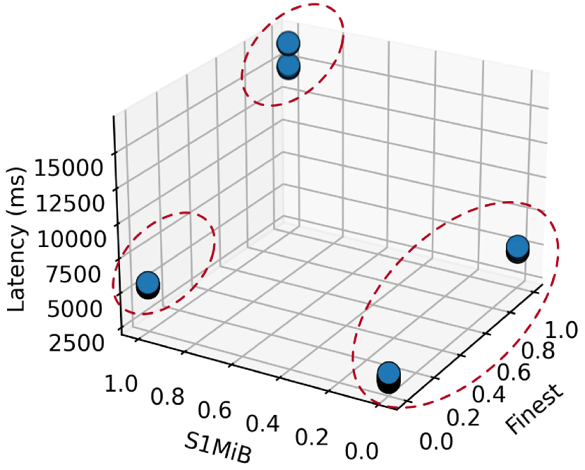
(a) BDB-J

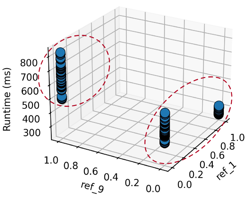
(b) x264

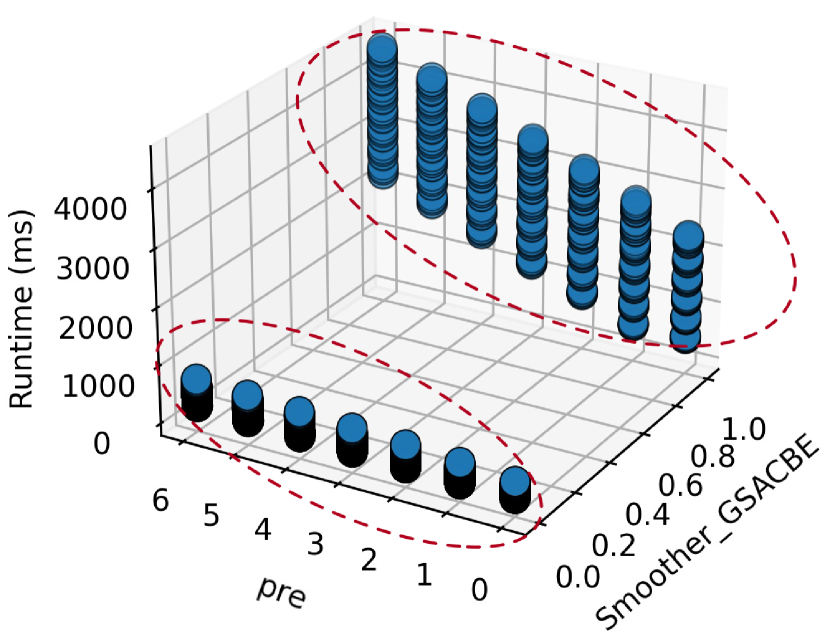
(c) HSMGP

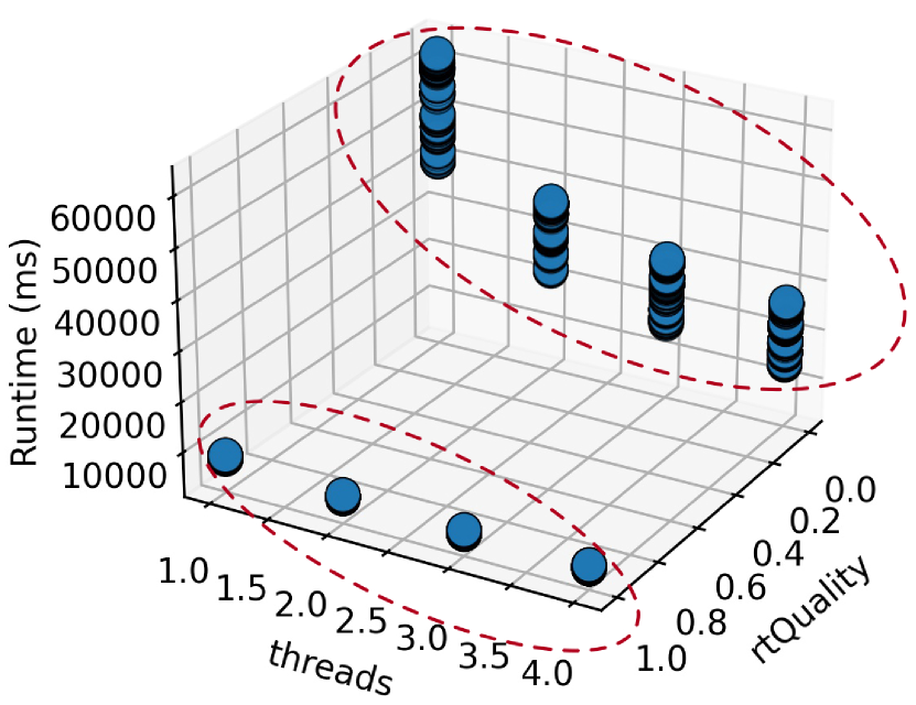
(d) VP8

Figure 1. Projection of configurations in the landscape with respect to the performance and two most important options (the divisions are circled).

2.2. Sparsity in Software Performance Learning

It has been known that the configuration space for software systems is generally rugged and sparse with respect to the configuration options (Jamshidi and Casale, 2016; Chen and Li, 2021; Ha and Zhang, 2019a; Chen, 2022a) — feature sparsity, which refers to the fact that only a small number of configuration options are prominent to the performance. We discover that, even with the key options that are the most influential to the performance, the samples still do not exhibit a “smooth” distribution over the configuration landscape. Instead, they tend to be spread sparsely: those with similar characteristics can form arbitrarily different divisions, which tend to be rather distant from each other. This is a typical case of high sample sparsity (Heck et al., 2022; Liu et al., 2020; Shibagaki et al., 2016) and it is often ignored in existing work for software performance learning.

In Figure 1, we show examples of the configuration samples measured from four real-world software systems. Clearly, we see that they all exhibit a consistent pattern—the samples tend to form different divisions with two properties:

• Property 1: configurations in the same division share closer performance values with smoother changes but those in-between divisions exhibit drastically different performance and can change more sharply.

• Property 2: configurations in the same division can have a closer value on at least one key option than those from the different divisions.

In this regard, the values of performance and key configuration options determine the characteristics of samples. In general, such a high sample sparsity is caused by two reasons: (1) the inherited consequence of high feature sparsity and (2) the fact that not all configurations are valid because of the constraints (e.g., an option can be used only if another option has been turned on) (Siegmund et al., 2015), thereby there are many “empty areas” in the configuration landscape.

When using machine learning models to learn concepts from the above configuration data, the model needs to (1) handle the complex interactions between the configuration options with high feature sparsity while (2) capture the diverse characteristics of configuration samples over all divisions caused by the high sample sparsity, e.g., in Figure 1, where samples in different divisions have diverged performance ranges. For the former challenge, there have been some approaches proposed to target such, such as DeepPerf (Ha and Zhang, 2019a) and Perf-AL (Shu et al., 2020). However, very little work has aimed to address the latter which can be the main obstacle for a model to learn and generalize the data for predicting the performance of the newly-given configuration. This is because those highly sparse samples increase the risk for models to overfit the training data, for instance by memorizing and biasing values in certain respective divisions (Heck et al., 2022), especially considering that we can often have limited samples from the configuration landscape due to the expensive measurement of configurable systems. The above is the main motivation of this work, for which we ask: how can we improve the accuracy of predicting software performance under such a high sample sparsity?

3. Divide-and-Learn for Performance Prediction

Drawing on our observations of the configuration data, we propose DaL — an approach that enables better prediction of the software performance via “divide-and-learn”. To mitigate the sample sparsity issue, the key idea of DaL is that, since different divisions of configurations show drastically diverse characteristics, i.e., rather different performance values with distant values of key configuration options, we seek to independently learn a local model for each of those divisions that contain locally smooth samples, thereby the learning can be more focused on the particular characteristics exhibited from the divisions and handle the feature sparsity. Yet, this requires us to formulate, on top of the original regression problem of predicting the performance value, a new classification problem without explicit labels. As such, we modify the original problem formulation (Equation 1) as below:

(2) $$\mathbfcal{D}=g(\mathbfcal{S})$$

(3) $$\forall D_{i}\in\mathbfcal{D}\text{: }\mathcal{P}=f(D_{i})\text{, }\mathcal{P}\in\mathbb{R}$$

Overall, we aim to achieve three goals:

• Goal 1: dividing the data samples into diverse yet more focused divisions $\mathbfcal{D}$ (building function $g$) and;

• Goal 2: training a dedicated local model for each division $D_{i}$ (building function $f$) while;

• Goal 3: assigning a newly coming configuration into the right model for prediction (using functions $g$ and $f$).

Figure 2 illustrates the overall architecture of DaL, in which there are three core phases, namely Dividing, Training, and Predicting. A pseudo code can also be found in Algorithm 1.

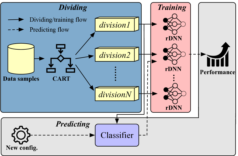
Figure 2. The architecture of DaL.

3.1. Dividing

The very first phase in DaL is to appropriately divide the data into more focused divisions while doing so by considering both the configuration options and performance values. To that end, the key question we seek to address is: how to effectively cluster the performance data with similar sample characteristics (Goal 1)?

Indeed, for dividing the data samples, it makes sense to consider various unsupervised clustering algorithms, such as $k$-mean (MacQueen et al., 1967), BIRCH (Zhang et al., 1996) or DBSCAN (Ester et al., 1996). However, we found that they are ill-suited for our problem, because:

• the distance metrics are highly system-dependent. For example, depending on the number of configuration options and whether they are binary/numeric options;

• it is difficult to combine the configuration options and performance value with appropriate discrimination;

• and clustering algorithms are often non-interpretable.

As a result, in DaL, we extend Classification and Regression Tree (CART) as the clustering algorithm (lines 3-11 in Algorithm 1) since (1) it is simple with interpretable/analyzable structure; (2) it ranks the important options as part of training (good for dealing with the feature sparsity issue), and (3) it does not suffer the issues above (Sarkar et al., 2015; Guo et al., 2018; Nair et al., 2018; Chen, 2019; Chen and Bahsoon, 2017; Nair et al., 2020; Guo et al., 2013). As illustrated in Figure 3, CART is originally a supervised and binary tree-structured model, which recursively splits some, if not all, configuration options and the corresponding data samples based on tuned thresholds. A split would result in two divisions, each of which can be further split. In this work, we at first train the CART on the available samples of configurations and performance values, during which we use the most common mean performance of all samples for each division $D_{i}$ as the prediction (Guo et al., 2018, 2013):

(4) $$\overline{y}_{D_{i}}={{1}\over{|D_{i}|}}{\sum_{y_{j}\in D_{i}}y_{j}}$$

in which $y_{j}$ is a performance value. For example, Figure 3 shows a projected example, in which the configuration that satisfies “rtQua- lity=true” and “threads=3” would lead to an inferred runtime of 112 seconds, which is calculated over all the 5 samples involved using Equation 4.

1

Input: The expected depth $d$ extracted from CART; a new configuration $\mathbf{\overline{c}}$ to be predicted

Output: The predicted performance of $\mathbf{\overline{c}}$

2

3if $\mathbfcal{M}=\emptyset$ then

4       /* dividing phase. */

5       $\mathbfcal{S}\leftarrow$ randomly sample a set of configurations and their performance

6       $\mathcal{T}\leftarrow$ trainCART($\mathbfcal{S}$)

7       $d^{\prime}=1$

8       while $d^{\prime}\leq d$ do

9             if $d^{\prime}<d$ then

10                   $\mathbfcal{D}\leftarrow$ extract all the leaf divisions of samples from $\mathcal{T}$ at the $d^{\prime}$th depth

11                  

12            else

13                   $\mathbfcal{D}\leftarrow$ extract all divisions of samples from $\mathcal{T}$ at the $d^{\prime}$th depth

14                  

15            $d^{\prime}=d^{\prime}+1$

16            

17      

18      /* training phase. */

19       for $D_{i}\in\mathbfcal{D}$ do

20             $\mathbfcal{M}\leftarrow$ trainRegularizedDNN($D_{i}$)

21            

22      

23

24/* predicting phase. */

25 if $\mathcal{F}$ has not been trained then

26       $\mathbfcal{U}\leftarrow$ Removing performance data and labeling the configurations based on their divisions in $\mathbfcal{D}$

27       $\mathbfcal{U^{\prime}}\leftarrow$ SMOTE($\mathbfcal{U}$)

28       $\mathcal{F}\leftarrow$ trainRandomForest($\mathbfcal{U^{\prime}}$)

29

30$D_{i}=$ predict($\mathcal{F}$,$\mathbf{\overline{c}}$)

31 $\mathcal{M}=$ get the model from $\mathbfcal{M}$ that corresponds to the predicted division $D_{i}$

32

33return predict($\mathcal{M}$,$\mathbf{\overline{c}}$)

34

Algorithm 1 Pseudo code of DaL

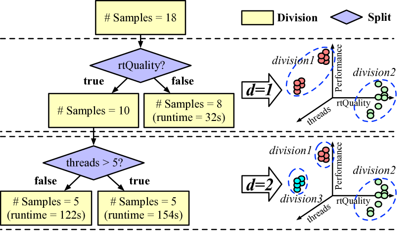
Figure 3. Projection of CART for VP8 showing the possible divisions with different colors under alternative depth $d$.

By choosing/ranking options that serve as the splits and tuning their thresholds, in DaL, we seek to minimize the following overall loss function during the CART training:

(5) $$\mathcal{L}={1\over{|D_{l}|}}{\sum_{y_{j}\in D_{l}}{(y_{j}-\overline{y}_{D_{l}})}^{2}}+{1\over{|D_{r}|}}{\sum_{y_{j}\in D_{r}}{(y_{j}-\overline{y}_{D_{r}})}^{2}}$$

where $D_{l}$ and $D_{r}$ denote the left and right division from a split, respectively. This ensures that the divisions would contain data samples with similar performance values (Property 1) while they are formed with respect to the similar values of the key configuration options as determined by the splits/thresholds at the finest granularity (Property 2), i.e., the more important options would appear on the higher level of the tree with excessive splitting.

However, here we do not use CART to generalize prediction directly on new data once it is trained as it has been shown that the splits and simple average of performance values in the division alone can still fail to handle the complex interactions between the options, leading to insufficient accuracy (Ha and Zhang, 2019a). Further, with our loss function in Equation 5, CART is prone to be overfitting especially for software quality data (Khoshgoftaar and Allen, 2001). This exacerbates the issue of sample sparsity (Heck et al., 2022) under a small amount of data samples which is not uncommon for configurable software systems (Ha and Zhang, 2019a; Shu et al., 2020).

Instead, what we are interested in are the (branch and/or leaf) divisions made therein (with respect to the training data), which enable us to use further dedicated and more focused local models for better generalizing to the new data (lines 6-11 in Algorithm 1). As such, the final prediction is no longer a simple average while we do not care about the CART overfitting itself as long as it fits the training data well. This is similar to the case of unsupervised clustering for which the clustering is guided by implicit labels (via the loss function at Equation 5). Specifically, in DaL we extract the data samples according to the divisions made by the $d$th depth of the CART, including all the leaf divisions with depth smaller than $d$. An example can be seen from Figure 3, where $d$ is a controllable parameter to be given. In this way, DaL divides the data into a range of $[d+1,2^{d}]$ divisions ($d\geq 1$), each of which will be captured by a local model learned thereafter. Note that when the number of data samples in the division is less than the minimum amount required by a model, we merge the two divisions of the same parent node.

As a concrete example, from Figure 3, we see that there are two depths: when $d=1$ there would be two divisions (one branch and one leaf) with 10 and 8 samples respectively; similarly, when $d=2$ there would be three leaf divisions: two of each have 5 samples and one is the division with 8 samples from $d=1$ as it is a leaf. In this case, CART has detected that the rtQuality is a more important (binary) option to impact the performance, and hence it should be considered at a higher level in the tree. Note that for numeric options, e.g., threads, the threshold of splitting (threads $>5$) is also tuned as part of the training process of CART.

3.2. Training

Given the divisions produced by the Dividing phase, we train a local model for the samples from each division identified as part of Goal 2 (lines 12-14 in Algorithm 1). Theoretically, we can pair them with any model. However, as we will show in Section 5.2, the state-of-the-art regularized Deep Neural Network (rDNN) (Ha and Zhang, 2019a) (namely DeepPerf), published at ICSE’19, is the most effective one under DaL as it handles feature sparsity well for configurable software. Indeed, Ha and Zhang (Ha and Zhang, 2019a) showed that rDNN is more effective than the others even with small data samples when predicting software performance (in our study, we also evaluate the same systems with small training sample sizes as used in their work). Therefore, in DaL we choose rDNN as the underlying local model by default.

In this work, we adopt exactly the same structure and training procedure as those used by Ha and Zhang (Ha and Zhang, 2019a), hence we kindly refer interested readers to their work for the training details (Ha and Zhang, 2019a). Since the local models of the divisions are independent, we utilize parallel training as part of DaL.

3.3. Predicting

When a new configuration arrives for prediction, DaL chooses a model of division trained previously to infer its performance. Therefore, the question is: how to assign the new configuration to the right model (Goal 3)? A naive solution is to directly feed the configuration into the CART from the dividing phase and check which divisions it associates with. Yet, since the performance of the new configuration is unforeseen from the CART’s training data, this solution requires CART to generalize accurately, which, as mentioned, can easily lead to poor results because CART is overfitting-prone when directly working on new data (Khoshgoftaar and Allen, 2001).

Instead, by using the divided samples from the Dividing phase (which serves as pseudo labeled data), we train a Random Forest—a widely used classifier and is resilient to overfitting  (Valov et al., 2015; Queiroz et al., 2016; Chen et al., 2021)—to generalize the decision boundary and predict which division that the new configuration should be better assigned to (lines 15-21 in Algorithm 1). Again, in this way, we are less concerned about the overfitting issue of CART as long as it matches the patterns of training data well. This now becomes a typical classification problem but there are only pseudo labels to be used in the training. Using the example from Figure 3 again, if $d=1$ then the configurations in the 10 sample set would have a label “division1”; similarly, those in the 8 sample set would result in a label “division2”.

However, one issue we experienced is that, even with $d=1$, the sample size of the two divisions can be rather imbalanced, which severely harms the quality of the classifier trained. For example, when training BDB-C with 18 samples, the first split in CART can lead to two divisions with 14 and 4 samples, respectively. Therefore, before training the classifier we use Synthetic Minority Oversampling Technique (SMOTE) (Blagus and Lusa, 2013) to pre-process the pseudo label data, hence the division(s) with much less data (minority) can be more repeatedly sampled.

Finally, the classifier predicts a division whose local model would infer the performance of the new configuration.

3.4. Trade-off with the Number of Divisions

Since more divisions mean that the sample space is separated into more loosely related regions for dealing with the sample sparsity, one may expect that the accuracy will be improved, or at least, stay similar, thereby we should use the maximum possible $d$ from CART in the dividing phase. This, however, only exists in the “utopia case” where there is an infinite set of configuration data samples.

In essence, with the design of DaL, the depth $d$ will manage two conflicting goals that influence its accuracy:

1. greater ability to handle sample sparsity by separating the distant samples into divisions, each of which is learned by an isolated local model;

2. and a larger amount of data samples in each division for the local model to be able to generalize.

Clearly, a greater $d$ may benefit goal (1) but it will inevitably damage goal (2) since it is possible for CART to generate divisions with imbalanced sample sizes. As a result, we see $d$ as a value that controls the trade-off between the two goals, and neither a too small nor too large $d$ would be ideal, as the former would lose the ability to deal with sample sparsity while the latter would leave too little data for a local model to learn, hence produce negative noises to the overall prediction. Similar to the fact that we cannot theoretically justify how much data is sufficient for a model to learn the concept (Oyedare and Park, 2019), it is also difficult to prove how many divisions are sufficient for handling the sample sparsity in performance modeling. However, in Section 5.3, we will empirically demonstrate that there is a (upward) quadratic correlation between $d$ value and the error incurred by DaL due to the conflict between the above two goals.

4. Experiment Setup

Here, we delineate the settings of our evaluation. In this work, DaL is implemented based on Tensorflow and scikit-learn. All experiments were carried out on a machine with Intel Core i7 2GHz CPU and 16GB RAM.

Table 1. Details of the subject systems. ($|\mathbfcal{B}|$/$|\mathbfcal{N}|$) denotes the number of binary/numerical options, and $|\mathbfcal{C}|$ denotes the number of valid configurations (full sample size).

System $|\mathbfcal{B}|$/$|\mathbfcal{N}|$ Performance Description $|\mathbfcal{C}|$ Used by Apache 9/0 Maximum load Web server 192 (Ha and Zhang, 2019a; Guo et al., 2018; Shu et al., 2020) BDB-C 16/0 Latency (ms) Database (C) 2560 (Ha and Zhang, 2019a; Guo et al., 2018; Shu et al., 2020) BDB-J 26/0 Latency (ms) Database (Java) 180 (Ha and Zhang, 2019a; Guo et al., 2018; Shu et al., 2020) x264 16/0 Runtime (ms) Video encoder 1152 (Ha and Zhang, 2019a; Guo et al., 2018; Shu et al., 2020) HSMGP 11/3 Runtime (ms) Compiler 3456 (Ha and Zhang, 2019a; Siegmund et al., 2015) HIPA^cc 31/2 Runtime (ms) Compiler 13485 (Ha and Zhang, 2019a; Siegmund et al., 2015) VP8 9/4 Runtime (ms) Video encoder 2736 (Peng et al., 2021) Lrzip 9/3 Runtime (ms) Compression tool 5184 (Peng et al., 2021)

4.1. Research Questions

In this work, we comprehensively assess DaL by answering the following research questions (RQ):

• RQ1: How accurate is DaL compared with the state-of-the-art approaches for software performance prediction?

• RQ2: Can DaL benefit different models when they are used locally therein for predicting software performance?

• RQ3: What is the sensitivity of DaL’s accuracy to $d$?

• RQ4: What is the model building time for DaL?

We ask RQ1 to assess the effectiveness of DaL under different sample sizes against the state-of-the-art. Since the default rDNN in DaL is replaceable, we study RQ2 to examine how the concept of “divide-and-learn” can benefit any given local model and whether using rDNN as the underlying local model is the best option. In RQ3, we examine how the depth of division ($d$) can impact the performance of DaL. Finally, we examine the overall overhead of DaL in RQ4.

4.2. Subject Systems

We use the same datasets of all valid configurations from real-world systems as widely used in the literature (Shu et al., 2020; Ha and Zhang, 2019a; Siegmund et al., 2015; Guo et al., 2018; Peng et al., 2021). To reduce noise, we remove those that contain missing measurements or invalid configurations. As shown in Table 1, we consider eight configurable software systems with diverse domains, scales, and performance concerns. Some of those contain only binary configuration options (e.g., x264) while the others involve mixed options (binary and numeric), e.g., HSMGP, which can be more difficult to model (Ha and Zhang, 2019a).

The configuration data of all the systems are collected by prior studies using the standard benchmarks with repeated measurement (Shu et al., 2020; Ha and Zhang, 2019a; Siegmund et al., 2015; Guo et al., 2018; Peng et al., 2021). For example, the configurations of Apache—a popular Web server—are benchmarked using the tools Autobench and Httperf, where workloads are generated and increased until reaching the point before the server crashes, and then the maximum load is marked as the performance value (Guo et al., 2018). The process repeats a few times for each configuration to ensure reliability.

To ensure generalizability of the results, for each system, we follow the protocol used by existing work (Siegmund et al., 2012b; Ha and Zhang, 2019a; Shu et al., 2020) to obtain five sets of training sample size in the evaluation:

• Binary systems: We randomly sample $n$, $2n$, $3n$, $4n$, and $5n$ configurations and their measurements, where $n$ is the number of configuration options (Ha and Zhang, 2019a; Shu et al., 2020).

• Mixed systems: We leverage the sizes suggested by SPLCon-queror (Siegmund et al., 2012b) (a state-of-the-art approach) depending on the amount of budget.

The results have been illustrated in Table 2. All the remaining samples in the dataset are used for testing.

Table 2. The training sample sizes used. $n$ denotes the number of configuration options in a binary system.

System Size 1 Size 2 Size 3 Size 4 Size 5 Apache $n$ $2n$ $3n$ $4n$ $5n$ BDB-C $n$ $2n$ $3n$ $4n$ $5n$ BDB-J $n$ $2n$ $3n$ $4n$ $5n$ x264 $n$ $2n$ $3n$ $4n$ $5n$ HSMGP 77 173 384 480 864 HIPA^cc 261 528 736 1281 2631 VP8 121 273 356 467 830 Lrzip 127 295 386 485 907

4.3. Metric and Statistical Validation

4.3.1. Accuracy

For all the experiments, mean relative error (MRE) is used as the evaluation metric for prediction accuracy, since it provides an intuitive indication of the error and has been widely used in the domain of software performance prediction (Ha and Zhang, 2019a; Shu et al., 2020; Guo et al., 2018). Formally, the MRE is computed as:

(6) $$MRE={{1}\over{k}}\times{\sum^{k}_{t=1}{{|A_{t}-P_{t}|}\over{A_{t}}}}\times 100\%$$

whereby $A_{t}$ and $P_{t}$ denote the $t$th actual and predicted performance, respectively. To mitigate bias, all experiments are repeated for 30 runs via bootstrapping without replacement. Note that excluding replacement is a common strategy for the performance learning of configuration as it is rare for a model to learn from the same configuration sample more than once (Gong and Chen, 2022).

4.3.2. Statistical Test

Since our evaluation commonly involves comparing more than two approaches, we apply Scott-Knott test (Mittas and Angelis, 2013) to evaluate their statistical significance on the difference of MRE over 30 runs, as recommended by Mittas and Angelis (Mittas and Angelis, 2013). In a nutshell, Scott-Knott sorts the list of treatments (the approaches that model the system) by their median values of the MRE. Next, it splits the list into two sub-lists with the largest expected difference (Xia et al., 2018). For example, suppose that we compare $A$, $B$, and $C$, a possible split could be $\{A,B\}$, $\{C\}$, with the rank ($r$) of 1 and 2, respectively. This means that, in the statistical sense, $A$ and $B$ perform similarly, but they are significantly better than $C$. Formally, Scott-Knott test aims to find the best split by maximizing the difference $\Delta$ in the expected mean before and after each split:

(7) $$\Delta=\frac{|l_{1}|}{|l|}(\overline{l_{1}}-\overline{l})^{2}+\frac{|l_{2}|}{|l|}(\overline{l_{2}}-\overline{l})^{2}$$

whereby $|l_{1}|$ and $|l_{2}|$ are the sizes of two sub-lists ($l_{1}$ and $l_{2}$) from list $l$ with a size $|l|$. $\overline{l_{1}}$, $\overline{l_{2}}$, and $\overline{l}$ denote their mean MRE.

During the splitting, we apply a statistical hypothesis test $H$ to check if $l_{1}$ and $l_{2}$ are significantly different. This is done by using bootstrapping and $\hat{A}_{12}$ (Vargha and Delaney, 2000). If that is the case, Scott-Knott recurses on the splits. In other words, we divide the approaches into different sub-lists if both bootstrap sampling and effect size test suggest that a split is statistically significant (with a confidence level of 99%) and with a good effect $\hat{A}_{12}\geq 0.6$. The sub-lists are then ranked based on their mean MRE.

Table 3. The median and interquartile range of MRE, denoted as Med (IQR), for DaL and the state-of-the-art approaches for all the subject systems and training sizes over 30 runs. For each case, green cells mean DaL has the best median MRE; or red cells otherwise. The one(s) with the best rank ($r$) from the Scott-Knott test is highlighted in bold.

Approach Apache BDB-C BDB-J x264 HSMGP HIPA^cc VP8 Lrzip $r$ Med (IQR) $r$ Med (IQR) $r$ Med (IQR) $r$ Med (IQR) $r$ Med (IQR) $r$ Med (IQR) $r$ Med (IQR) $r$ Med (IQR) DeepPerf 3 20.19 (6.34) 1 43.66 (42.88) 3 2.98 (3.34) 2 8.04 (3.06) 3 7.09 (3.04) 2 9.70 (1.28) 2 4.68 (3.27) 2 35.40 (16.59) DECART 2 19.44 (6.48) 3 51.88 (45.91) 1 2.36 (0.75) 3 9.27 (2.11) N/A N/A N/A N/A N/A N/A N/A N/A Perf-AL 4 33.57 (11.34) 4 82.38 (57.27) 5 37.45 (2.45) 4 37.00 (9.43) 4 66.70 (14.05) 4 31.99 (0.06) 4 60.05 (2.03) 3 58.45 (0.12) SPLConqueror 1 14.44 (0.00) 4 86.85 (0.00) 4 12.29 (0.00) 1 7.01 (0.00) 2 15.04 (0.00) 3 16.68 (0.00) 3 29.39 (0.00) 4 123.7 (0.00) Size 1 DaL 2 21.02 (6.64) 1 41.77 (32.54) 2 3.14 (2.90) 2 8.04 (1.30) 1 4.66 (1.32) 1 9.07 (1.18) 1 1.59 (0.36) 1 26.40 (6.94) DeepPerf 1 9.79 (4.56) 2 18.17 (8.11) 2 1.91 (0.68) 1 3.17 (1.00) 2 3.69 (0.61) 2 6.89 (1.44) 2 2.39 (1.21) 2 21.46 (4.53) DECART 2 9.77 (5.36) 1 13.37 (7.25) 1 1.84 (0.17) 2 6.29 (1.72) N/A N/A N/A N/A N/A N/A N/A N/A Perf-AL 4 32.97 (6.24) 4 73.99 (22.51) 5 37.90 (1.67) 4 34.98 (7.81) 4 66.67 (0.11) 4 31.98 (0.06) 4 60.04 (0.24) 3 58.46 (0.18) SPLConqueror 3 13.88 (0.00) 2 162.91 (0.00) 4 24.85 (0.00) 3 6.63 (0.00) 3 22.63 (0.00) 3 16.96 (0.00) 3 35.34 (0.00) 4 171.85 (0.00) Size 2 DaL 2 9.82 (5.39) 3 17.22 (15.67) 3 1.90 (0.37) 1 3.21 (1.95) 1 2.66 (0.68) 1 5.55 (0.60) 1 1.21 (0.09) 1 15.37 (6.04) DeepPerf 2 7.98 (1.91) 2 12.47 (4.08) 3 2.01 (1.10) 2 2.23 (0.90) 2 2.28 (0.37) 2 4.68 (0.90) 2 1.93 (0.72) 2 18.68 (3.20) DECART 2 8.07 (1.05) 1 7.56 (5.07) 1 1.64 (0.24) 3 4.57 (1.03) N/A N/A N/A N/A N/A N/A N/A N/A Perf-AL 4 31.73 (4.66) 2 69.74 (4.33) 5 37.19 (1.70) 5 36.25 (7.73) 4 66.63 (0.18) 4 31.99 (0.06) 4 60.02 (0.29) 3 58.44 (0.21) SPLConqueror 3 13.99 (0.00) 3 193.89 (0.00) 4 25.88 (0.00) 4 6.31 (0.00) 3 32.46 (0.00) 3 17.18 (0.00) 3 36.26 (0.00) 4 177.61 (0.00) Size 3 DaL 1 7.17 (2.67) 1 5.74 (6.84) 2 1.61 (0.31) 1 1.66 (0.57) 1 1.56 (0.20) 1 4.39 (0.41) 1 1.12 (0.08) 1 11.83 (4.53) DeepPerf 1 6.85 (1.60) 2 9.06 (9.76) 3 1.70 (0.37) 2 1.74 (0.98) 2 2.23 (0.39) 2 3.58 (1.00) 2 1.54 (0.40) 2 15.55 (1.71) DECART 2 7.47 (0.72) 1 5.17 (5.07) 1 1.47 (0.12) 3 3.66 (1.42) N/A N/A N/A N/A N/A N/A N/A N/A Perf-AL 4 30.67 (6.84) 3 69.50 (2.49) 5 37.74 (2.59) 5 36.41 (6.47) 4 66.63 (0.14) 4 31.98 (0.06) 4 59.99 (0.27) 3 58.48 (0.21) SPLConqueror 3 13.84 (0.00) 4 231.68 (0.00) 4 29.01 (0.00) 4 6.32 (0.00) 3 33.73 (0.00) 3 17.42 (0.00) 3 37.14 (0.00) 4 236.48 (0.00) Size 4 DaL 1 6.59 (1.77) 1 3.68 (2.78) 2 1.61 (0.29) 1 1.13 (0.63) 1 1.49 (0.15) 1 3.22 (0.35) 1 1.10 (0.06) 1 10.10 (3.23) DeepPerf 2 6.66 (1.61) 2 7.08 (8.03) 2 1.69 (0.48) 2 1.44 (0.90) 2 1.94 (0.68) 2 2.82 (0.57) 2 1.45 (0.23) 2 10.17 (0.91) DECART 3 7.14 (0.89) 1 3.54 (1.92) 1 1.37 (0.26) 3 2.15 (1.05) N/A N/A N/A N/A N/A N/A N/A N/A Perf-AL 5 30.45 (4.91) 3 69.29 (0.69) 4 35.76 (4.47) 5 36.20 (3.75) 4 66.59 (0.20) 4 31.97 (0.14) 4 59.95 (0.68) 3 58.39 (0.21) SPLConqueror 4 14.06 (0.00) 4 296.68 (0.00) 3 29.87 (0.00) 4 6.36 (0.00) 3 35.86 (0.00) 3 17.69 (0.00) 3 36.21 (0.00) 4 208.08 (0.00) Size 5 DaL 1 5.96 (2.07) 1 2.15 (1.52) 1 1.46 (0.26) 1 0.79 (0.33) 1 1.16 (0.08) 1 2.39 (0.22) 1 1.07 (0.05) 1 6.60 (1.34)

5. Evaluation

5.1. Comparing with the State-of-the-art

5.1.1. Method

To understand how DaL performs compared with the state-of-the-art, we assess its accuracy against both the standard approaches that rely on statistical learning, i.e., SPLConqueror (Siegmund et al., 2012b) (linear regression and sampling methods) and DECART (Guo et al., 2018) (an improved CART), together with recent deep learning-based ones, i.e., DeepPerf (Ha and Zhang, 2019a) (a single global rDNN) and Perf-AL (Shu et al., 2020) (an adversarial learning method). All approaches can be used for any type of system except for DECART, which works on binary systems only. Following the setting used by Ha and Zhang (Ha and Zhang, 2019a), SPLConqueror and DECART use their own sampling method while DaL, DeepPerf and Perf-AL rely on random sampling. Since there are 8 systems and 5 sample sizes each, we obtain 40 cases to compare in total.

We use the implementations published by their authors with the same parameter settings. For DaL, we set $d=1$ or $d=2$ depending on the systems, which tends to be the most appropriate value based on the result under a small portion of training data (see Section 5.3). We use the systems, training sizes, and statistical tests as described in Section 4. All experiments are repeated for 30 runs.

5.1.2. Results

The results have been illustrated in Table 3, from which we see that DaL remarkably achieves the best accuracy on 31 out of 40 cases. In particular, DaL considerably improves the accuracy, e.g., by up to $1.94\times$ better than the second-best one on Size 1 of VP8. The above still holds when looking into the results of the statistical test: DaL is the only approach that is ranked first for 26 out of the 31 cases. For the 9 cases where DaL does not achieve the best median MRE, it is equally ranked as the first for two of them. These conclude that DaL is, in 33 cases, similar to (7 cases) or significantly better (26 cases) than the best state-of-the-art for each specific case (which could be a different approach).

For cases with different training sample sizes, we see that DaL performs generally more inferior than the others when the size is too limited, i.e., Size 1 and Size 2 for the binary systems. This is expected as when there are too few samples, each local model would have a limited chance to observe the right pattern after the splitting, hence blurring its effectiveness in handling sample sparsity. However, in the other cases (especially for mixed systems that have more data even for Size 1), DaL needs far fewer samples to achieve the same accuracy as the best state-of-the-art. For example, on Lrzip, DaL only needs 386 samples (Size 3) to achieve an error less than 15% while DeepPerf requires 907 samples (Size 5) to do so.

Another observation is that the improvements of DaL is much more obvious in mixed systems than those for binary systems. This is because: (1) the binary systems have fewer training samples as they have a smaller configuration space. Therefore, the data learned by each local model is more restricted. (2) The issue of sample sparsity is more severe on mixed systems, as their configuration landscape is more complex and comes with finer granularity.

As a result, we anticipate that the benefit of DaL can be amplified with more complex systems and/or more training data.

Table 4. The Scott-Knott ranks ($r$) on the MRE of DaL under different local models and their global counterparts. The green cells denote the best rank. Raw MRE results can be accessed at: https://github.com/ideas-labo/DaL/blob/main/Table4_full.pdf.

System DaL rDNN DaL_RF RF DaL_CART CART DaL_LR LR DaL_SVR SVR DaL_KRR KRR DaL_kNN $k$NN Apache Size 1 1 2 1 3 2 2 1 5 4 4 6 7 2 2 Size 2 2 1 2 2 2 1 3 5 6 7 8 9 4 6 Size 3 1 2 3 2 4 4 1 7 6 9 10 11 5 8 Size 4 2 2 3 2 5 4 1 8 7 9 10 11 6 8 Size 5 2 4 4 3 5 5 1 9 7 10 11 12 6 8 BDB-C Size 1 2 2 2 6 1 1 3 8 3 4 2 7 3 5 Size 2 1 1 3 4 1 2 7 6 5 5 4 6 5 6 Size 3 2 5 4 4 3 1 6 9 8 7 6 9 8 9 Size 4 1 3 3 4 1 2 5 9 6 6 5 8 6 7 Size 5 1 3 2 4 1 1 4 9 6 7 5 9 6 8 BDB-J Size 1 2 2 2 3 1 1 9 8 6 4 3 7 5 5 Size 2 4 3 1 1 3 2 4 10 8 5 4 9 6 7 Size 3 2 3 1 1 2 2 3 8 6 5 3 7 4 4 Size 4 2 4 1 1 3 3 4 9 8 8 5 9 7 6 Size 5 2 4 1 1 3 3 4 9 7 8 5 9 6 6 x264 Size 1 1 1 3 2 3 3 4 5 5 9 8 6 4 7 Size 2 1 1 3 3 3 3 2 4 7 9 4 5 6 8 Size 3 1 2 5 5 4 4 2 5 6 9 5 7 8 9 Size 4 1 2 5 6 3 4 3 7 7 10 6 8 9 11 Size 5 1 2 5 6 3 4 6 8 8 11 7 9 10 12 HSMGP Size 1 1 8 6 5 7 7 2 11 4 5 3 10 8 9 Size 2 1 2 5 6 8 8 2 10 7 8 4 10 9 9 Size 3 1 2 4 5 7 7 2 10 6 9 3 10 8 8 Size 4 1 2 3 4 7 8 4 11 6 10 5 11 9 9 Size 5 1 2 3 3 7 6 10 9 4 8 5 10 9 9 HIPA^cc Size 1 1 2 3 3 4 4 9 8 5 7 4 9 6 8 Size 2 1 2 3 3 3 3 6 10 5 6 5 8 4 7 Size 3 1 2 3 3 3 3 5 11 5 8 6 10 4 9 Size 4 1 2 4 4 3 3 8 11 7 10 8 11 6 5 Size 5 1 2 3 2 2 2 10 12 7 8 9 11 5 6 VP8 Size 1 1 5 4 6 2 3 5 7 9 10 7 12 10 11 Size 2 4 5 3 4 1 2 4 8 6 11 7 12 9 10 Size 3 1 2 2 2 2 3 5 11 5 9 6 10 8 8 Size 4 1 2 2 2 2 2 3 8 4 6 3 7 5 6 Size 5 1 2 3 4 2 3 6 12 7 10 5 11 8 9 Lrzip Size 1 3 4 2 3 1 2 5 10 5 5 7 9 6 5 Size 2 3 4 2 2 1 2 5 8 6 6 7 9 5 5 Size 3 3 4 2 1 1 2 6 9 7 6 8 10 5 5 Size 4 3 4 4 7 1 2 8 10 2 3 6 9 5 8 Size 5 3 4 1 3 1 2 7 9 7 8 9 11 5 6 Average 1.63 2.78 2.90 3.38 2.95 3.15 4.63 8.58 6.00 7.48 5.85 9.13 6.25 7.35

To summarize, we can answer RQ1 as:

5.2. DaL under Different Local Models

5.2.1. Method

Since the idea of “divide-and-learn” can be applicable to a wide range of underlying local models of the divisions identified, we seek to understand how well DaL perform with different local models against their global model counterparts (i.e., using them directly to learn the entire training dataset). To that end, we run experiments on a set of global models available in scikit-learn and widely used in software engineering tasks to make predictions directly (Li et al., 2020; Gong and Chen, 2022), such as CART, Random Forest (RF), Linear Regression (LR), Support Vector Regression (SVR), Kernel Ridge Regression (KRR), and $k$-Nearest Neighbours ($k$NN). We used the same settings as those for RQ1 and all models’ hyperparameters are tuned in training. For the simplicity of exposition, we report on the ranks $r$ produced by the Scott-Knott test.

5.2.2. Result

From Table 4, we can obtain the following key observations: firstly, when examining each pair of the counterparts, i.e., DaL_X and X, DaL can indeed improve the accuracy of the local model via the concept of “divide-and-learn”. In particular, for simple but commonly ineffective models like LR (Ha and Zhang, 2019a), DaL can improve them to a considerable extent. Yet, we see that DaL does not often lead to a significantly different result when working with CART against using CART directly. This is as expected, since using different CART models for the divisions identified by a CART makes little difference to applying a single CART that predicts directly. Interestingly, we also see that our model performs better than the traditional ensemble learning: DaL_CART—a CART-based “divide-and-learn” model performs generally better than RF, which uses CART as the local model and combines them via Bagging.

Secondly, the default of DaL, which uses the rDNN as the local model, still performs significantly better than the others. This aligns with the findings from existing work (Ha and Zhang, 2019a) that the rDNN handles the feature sparsity better. Indeed, deep learning models are known to be data-hungry, but our results surprisingly show that they can also work well for a limited amount of configuration samples. The key behind such is the use of regularization, which stresses additional penalties on the more important weights/options. This has helped to relieve the need for a large amount of data during training while better fitting with the sparse features in configuration data. A similar conclusion has also been drawn from previous studies (Ha and Zhang, 2019a).

Therefore, for RQ2, we say:

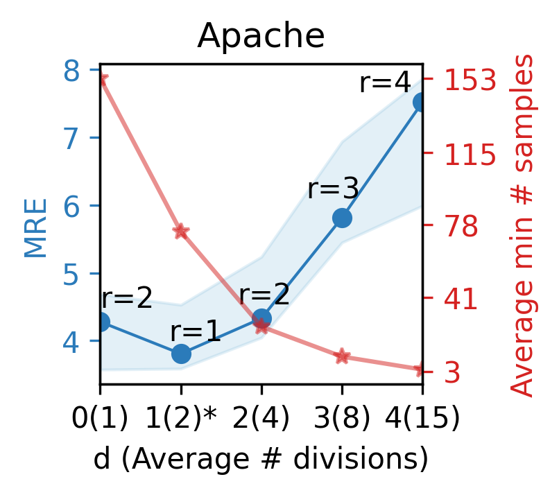
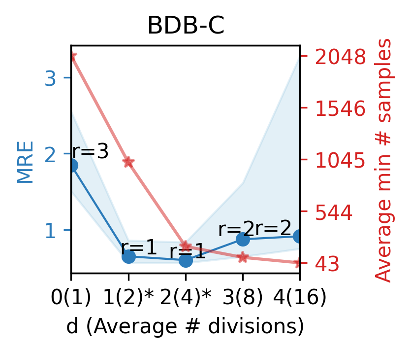
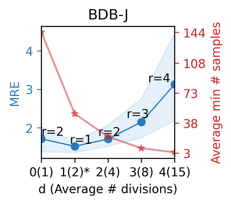
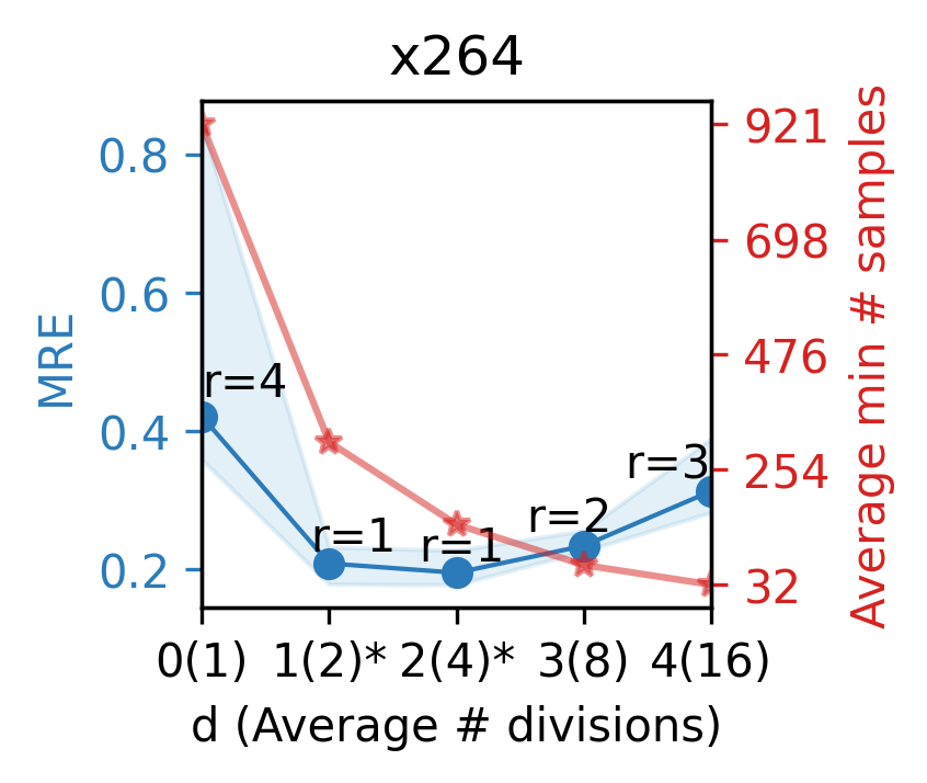
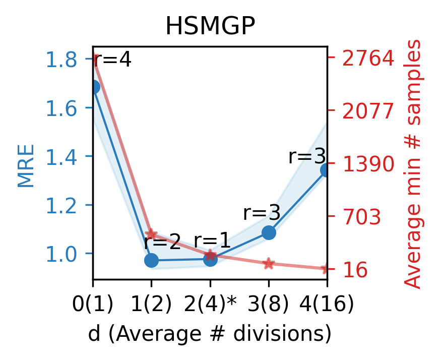
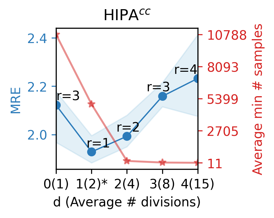
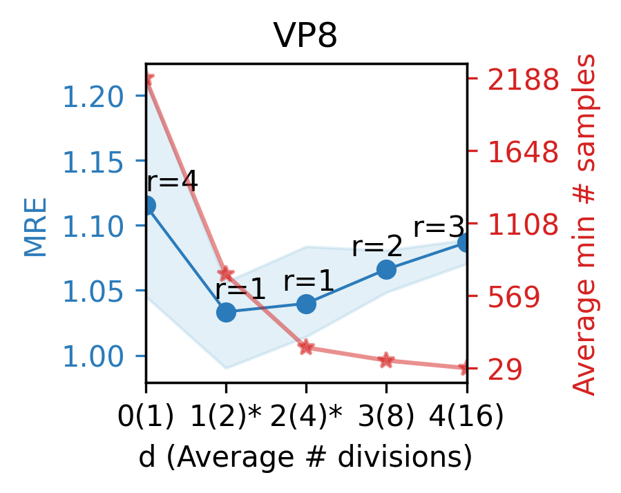
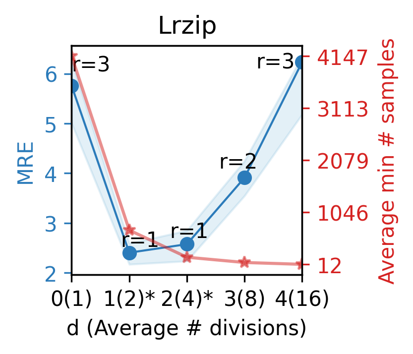
Figure 4. The median MRE ( ), its IQR (area), and the average smallest training size of the divisions ( ) achieved by DaL under different depths ($d$ values)/number of divisions over all systems and 30 runs. $r=1$ means rank 1 in the Scott-Knott test on MRE. The best-ranked $d$ is marked as $*$.

5.3. Sensitivity to the Depth $d$

5.3.1. Method

To understand RQ3, we examine different $d$ values. Since the number of divisions (and hence the possible depth) is sample size-dependent, for each system, we use 80% of the full dataset for training and the remaining for testing. This has allowed us to achieve up to $d=4$ with 16 divisions as the maximum possible bound. For different $d$ values, we report on the median MRE together with the results of Scott-Knott test for 30 runs. We also report the smallest sample size from the divisions, averaging over 30 runs.

5.3.2. Results

From Figure 4, we see that the correlation between the error of DaL and $d$ value is close to quadratic: DaL reaches its best MRE with $d=1$ or $d=2$. At the same time, the size of training data for a local model decreases as the number of divisions increases. Since $d$ controls the trade-off between the ability to handle sample sparsity and ensuring sufficient data samples to train all local models, $d=1$ or $d=2$ tends to be the “sweet points” that reach a balance for the systems studied. After the point of $d=1$ or $d=2$, the MRE will worsen, as the local models’ training size often drops dramatically. This is a clear sign that, from that point, the side-effect of having too less samples to train a local model has started to surpass the benefit that could have been brought by dealing with sample sparsity using more local models.

When $d=0$, which means only one division and hence DaL is reduced to DeepPerf that ignores sample sparsity, the resulted MRE is the worst on 4 out of 8 systems; the same applied to the case when $d=4$. This suggests that neither too small $d$ (e.g., $d=0$ with only one division) nor too larger $d$ (e.g., $d=4$ with up to 16 divisions, i.e., too many divisions) are ideal, which matches our theoretical analysis in Section 3.4.

Therefore, we conclude that:

5.4. Overhead of Model Building

5.4.1. Method

To study RQ4, we examine the overall time required and the breakdown of overhead for DaL in various phases. As some baselines, we also illustrate the model building time required by the approaches compared in RQ1.

5.4.2. Result

Table 5. The overhead ranges across all systems and sizes.

Approach Overhead (min) Restriction and Prerequisite DeepPerf 3 to 60 None DECART 0.07 to 0.5 does not work on mixed systems Perf-AL 0.08 to 1 None SPLConqueror 4$\times 10^{-4}$ to 5$\times 10^{-3}$ needs to select sampling method(s) DaL 6 to 56 needs to set the depth $d$ — DaL (dividing) 9$\times 10^{-4}$ to 0.18 None — DaL (training) 4 to 52 None — DaL (predicting) 1.3 to 5 None

From Table 5, DaL incurs an overall overhead from 6 to 56 minutes. Yet, from the breakdown, we note that the majority of the overhead comes from the training phase that trains the local models. This is expected, as DaL uses rDNN by default.

Specifically, the overhead of DaL compared with DeepPerf (3 to 60 minutes) is encouraging as it tends to be faster in the worst-case scenario while achieving up to $1.94\times$ better accuracy. This is because (1) each local model has less data to train and (2) the parallel training indeed speeds up the process. In contrast to Perf-AL (a few seconds to one minute), DaL appears to be rather slow as the former does not use hyperparameter tuning but fixed-parameter values (Shu et al., 2020). Yet, as we have shown for RQ1, DaL achieves up to a few magnitudes of accuracy improvement. Although SPLConqueror and DECART have an overhead of less than a minute, again their accuracy is much more inferior. Further, SPLConqueror requires a good selection of the sampling method(s) (which can largely incur additional overhead) while DECART does not work on mixed systems. Finally, we have shown in RQ3 that DaL’s MRE is quadratically sensitive to $d$ (upward), hence its value should be neither too small nor too large, e.g., $d=1$ or $d=2$ in this work.

In summary, we say that:

6. Discussion

6.1. Why does DaL Work?

To provide a more detailed understanding of why DaL performs better than state-of-the-art, in Figure 5, we showcase the most common run of the predicted performance by DaL and DeepPerf against actual performance. Clearly, we note that the sample sparsity is rather obvious where there are two distant divisions. DeepPerf, as an approach that relies on a single and global rDNN, has been severely affected by such highly sparse samples: we see that the model tries to cover points in both divisions, but fails to do so as it tends to overfit the points in one or the other. This is why, in Figure 5b, its prediction on some configurations that should lead to low runtime tend to have much higher values (e.g., when rtQuality=1 and threads=1) while some of those that should have high runtime may be predicted with much lower values (e.g., when rtQuality=0 and threads=1). DaL, in contrast, handles such a sample sparsity well as it contains different local models that particularly cater to each division identified, hence leading to high accuracy (Figure 5a).

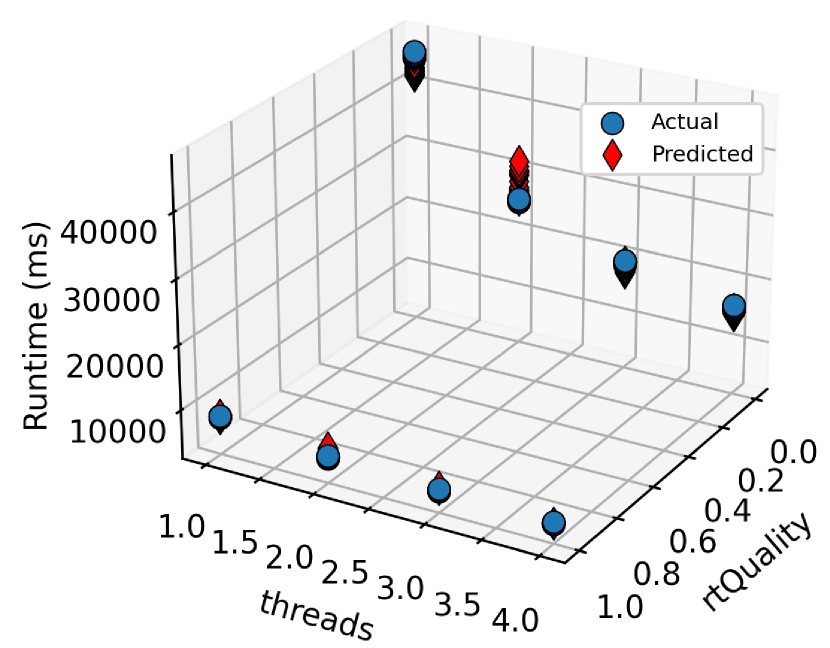
(a) prediction by DaL

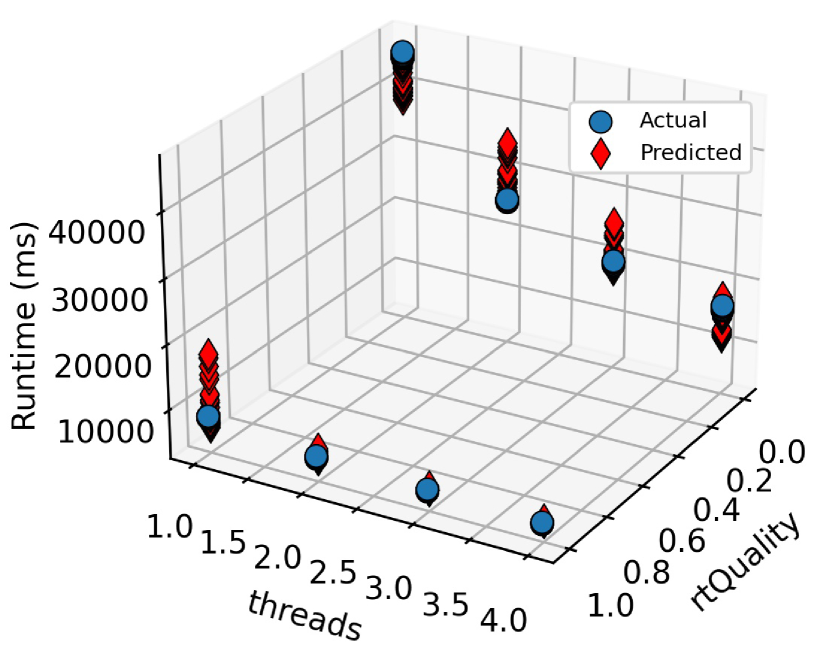
(b) prediction by DeepPerf

Figure 5. Example run of the actual and predicted performance by DaL and DeepPerf for VP8.

6.2. Strengths and Limitations

The first strength of DaL is that the concept of “divide-and-learn”, paired with the rDNN, can handle both sample sparsity and feature sparsity well. As from Section 5.1 for RQ1, this has led to better accuracy and better utilization of the sample data than the state-of-the-art approaches.

The second strength is that, as from Section 5.2 for RQ2, DaL can improve different local models compared with when they are used alone as a global model. While we set rDNN as the default for the best accuracy, one can also easily replace it with others such as LR for faster training and better interoperability. This enables great flexibility with DaL to make trade-offs on different concerns of the practical scenarios.

A limitation of DaL is that it takes a longer time to build the model than some state-of-the-art approaches. On a machine with CPU 2GHz and 16GB RAM, DaL needs between 6 and 56 minutes for systems with up to 33 options and more than 2,000 samples.

6.3. Why $d\in\{1|2\}$ is Highly Effective?

We have shown that the setting of $d$ in DaL should be neither too small nor too large; the key intention behind the $d$ is to reach a good balance between handling the sample sparsity and providing sufficient data for the local models to generalize. This is especially true when the CART might produce divisions with imbalanced sample sizes, e.g., we observed cases where there is a division with around 500 samples while one other has merely less than 10. Our experimental results show that such “sweet points” tend to be $d=1$ or $d=2$ for the cases studied in this work.

However, the notion of “too small” and “too large” should be interpreted cautiously depending on the systems and data size. That is, although in this study, setting $d=1$ or $d=2$ appears to be appropriate; they might become “too small” settings when the data size increases considerably and/or the system naturally exhibits well-balanced divisions of configuration samples in the landscapes. Yet, the pattern of quadratic correlation between $d$ and the error of DaL should remain unchanged.

6.4. Using DaL in Practice

Like many other data-driven approaches, using DaL is straightforward and free of assumptions about the software systems, data, and environments. We would recommend setting $d=1$ or $d=2$ by default, especially when the data sample size is similar to those we studied in this work. Of course, it is always possible to fine-tune the $d$ value by training DaL with alternative settings under the configuration samples available. Given the quadratic correlation between $d$ and the error, it is possible to design a simple heuristic for this, e.g., we compare the accuracy of DaL trained with $d=i$ and $d=i+1$ starting from $d=1$ and finally selecting the maximum $d$ value $k$ such that DaL with $k+1$ is less accurate than DaL with $k$.

6.5. Threats to Validity

Internal Threats. Internal threats to validity are related to the parameters used. In this work, we set the same setting as used in state-of-the-art studies (Siegmund et al., 2012b; Guo et al., 2013; Ha and Zhang, 2019a; Shu et al., 2020). We have also shown the sensitivity of DaL to $d$ and reveal that there exists a generally best setting. We repeat the experiments for 30 runs and use Scott-Knott test for multiple comparisons.

Construct Threats. Threats to construct validity may lie in the metric used. In this study, MRE is chosen for two reasons: (1) it is a relative metric and hence is insensitive to the scale of the performance; (2) MRE has been recommended for performance prediction by many latest studies (Ha and Zhang, 2019a; Shu et al., 2020; Guo et al., 2018).

External Threats. External validity could be raised from the subject systems and training samples used. To mitigate such, we evaluate eight commonly used subject systems selected from the latest studies. We have also examined different training sample sizes as determined by SPLConqueror (Siegmund et al., 2012b)—a typical method. Yet, we agree that using more subject systems and data sizes may be fruitful, especially for examining the sensitivity of $d$ which may lead to a different conclusion when there is a much larger set of training configuration samples than we consider in this study.

7. Related Work

We now discuss the related work in light of DaL.

Analytical model. Predicting software performance can be done by analyzing the code structure and architecture of the systems (Di Marco and Inverardi, 2004; Velez et al., 2021). For example, Marco and Inverardi (Di Marco and Inverardi, 2004) apply queuing network to model the latency of requests processed by the software. Velez et al. (Velez et al., 2021) use local measurements and dynamic taint analysis to build a model that can predict performance for part of the code. However, analytical models require full understanding and access to the software’s internal states, which may not always be possible/feasible. DaL is not limited to those scenarios as it is a data-driven approach.

Statistical learning-based model. Data-driven learning has relied on various statistical models, such as linear regressions (Siegmund et al., 2012b, 2015; Sun et al., 2020; Kang et al., 2020), tree-liked model (Hsu et al., 2018; Sarkar et al., 2015; Nair et al., 2020), and fourier-learning models (Zhang et al., 2015; Ha and Zhang, 2019b), etc. Among others, SPLConqueror (Siegmund et al., 2012b) utilizes linear regression combined with different sampling methods and a step-wise feature selection to capture the interactions between configuration options. DECART (Guo et al., 2018) is an improved CART with an efficient sampling method (Zhang et al., 2015). However, recent work reveals that those approaches do not work well with small datasets (Ha and Zhang, 2019a), which is rather common for configurable software systems due to their expensive measurements. This is a consequence of not fully handling the sparsity in configuration data. Further, they come with various restrictions, e.g., DECART does not work on mixed systems while SPLConqueror needs an extensive selection of the right sampling method(s). In contrast, we showed that DaL produces significantly more accurate results while does not limit to those restrictions.

Ensemble model. Models can be combined in a shared manner to predict software performance. For example, Chen and Bahsoon (Chen and Bahsoon, 2017) propose an ensemble approach, paired with feature selection for mitigating feature sparsity, to model software performance. Other classic ensemble learning models such as Bagging (Breiman, 1996) and Boosting (Schapire, 2003) (e.g., RF) can also be equally adopted. Indeed, at a glance, our DaL does seem similar to the ensemble model as they all maintain a pool of local models. However, the key difference is that the classic ensemble models will inevitably share information between the local models at one or more of the following levels:

• At the training level, e.g., the local models in Boosting learn the same samples but with a different focus; the Bucket of Models (i.e., what Chen and Bahsoon (Chen and Bahsoon, 2017) did) builds local models on the same data and uses the best upon prediction.

• At the model prediction level, e.g., Bagging aggregates the results of local models upon prediction.

DaL, in contrast, has no information sharing throughout the learning as the samples are split and so does the prediction of the local models. This has enabled it to better isolate the samples and cope with their inherited sparsity, e.g., recall from RQ2, the overall accuracy of DaL_CART is better than RF (they both use CART as the local models but learn with and without sharing information).

Deep learning-based model. A variety of studies apply neural network with multiple layers and/or ensemble learning to predict software performance (Ha and Zhang, 2019a; Shu et al., 2020; Nemirovsky et al., 2017; Sohail et al., 2021; Falch and Elster, 2017; Kim et al., 2017; Marathe et al., 2017; Johnsson et al., 2019; Zhang et al., 2018). DeepPerf (Ha and Zhang, 2019a) is a state-of-the-art DNN model with $L_{1}$ regularization to mitigate feature sparsity for any configurable systems, and it can be more accurate than many other existing approaches. The most recently proposed Perf-AL (Shu et al., 2020) relied on adversarial learning, which consists of a generative network to predict the performance and a discriminator network to distinguish the predictions and the actual labels. Nevertheless, existing deep learning approaches capture only the feature sparsity while ignoring the sample sparsity, causing serve risks of overfitting even with regularization in place. Compared with those, we have shown that, by capturing sample sparsity, DaL is able to improve the accuracy considerably with better efficiency and acceptable overhead.

Hybrid model. The analytical models can be combined with data-driven ones to form a hybrid model (Han et al., 2021; Didona et al., 2015; Weber et al., 2021). Among others, Didona et al. (Didona et al., 2015) use linear regression and $k$NN to learn certain components of a queuing network. Conversely, Weber et al. (Weber et al., 2021) propose to learn the performance of systems based on the parsed source codes from the system to the function level. We see DaL as being complementary to those hybrid models due to its flexibility in selecting the local model: when needed, the local models can be replaced with hybrid ones, making itself a hybrid variant. In case the internal structure of the system is unknown, DaL can also work in its default as a purely data-driven approach.

8. Conclusion

This paper proposes DaL, an approach that effectively handles the sparsity issues in configurable software performance prediction. By formulating a classification problem with pseudo labels on top of the original regression problem, DaL extracts the branches/leaves from a CART which divides the samples of configuration into distant divisions and trains a dedicated local rDNN for each division thereafter. Prediction of the new configuration is then made by the rDNN of division inferred by a Random Forest classifier. As such, the division of samples and the trained local model handles the sample sparsity while the rDNN deals with the feature sparsity.

We evaluate DaL on eight real-world systems that are of diverse domains and scales, together with five sets of training data. The results show that DaL is:

• effective as it is competitive to the best state-of-the-art approach on 33 out of 40 cases, in which 26 of them are significantly better with up to $1.94\times$ MRE improvement;

• efficient since it often requires fewer samples to reach the same/better accuracy compared with the state-of-the-art;

• flexible given that it considerably improves various global models when they are used as the local model therein;

• robust because, given the quadratic correlation, a middle $d$ value(s) (between 0 and the bound set by CART) can be robust and leads to the best accuracy across the cases, e.g., $d=1$ or $d=2$ under the sample sizes in this work.

Mitigating the issues caused by sparsity is only one step towards better performance prediction, hence the possible future work based on DaL is vast, including multi-task prediction of performance under different environments and merging diverse local models (e.g., a mix of rDNN and LR) as part of the “divide-and-learn” concept. Consolidating DaL with an adaptive $d$ is also within our agenda.

9. Data Availability

Data, code, and supplementary figures of this work can be found at our repository: https://github.com/ideas-labo/DaL.

References

- (1)
- Alpaydin (2004) Ethem Alpaydin. 2004. Introduction to machine learning.
- Blagus and Lusa (2013) Rok Blagus and Lara Lusa. 2013. SMOTE for high-dimensional class-imbalanced data. BMC Bioinform. 14 (2013), 106. https://doi.org/10.1186/1471-2105-14-106
- Breiman (1996) Leo Breiman. 1996. Bagging predictors. Machine learning 24 (1996), 123–140.
- Chen et al. (2021) Junjie Chen, Ningxin Xu, Peiqi Chen, and Hongyu Zhang. 2021. Efficient Compiler Autotuning via Bayesian Optimization. In 43rd IEEE/ACM International Conference on Software Engineering, ICSE 2021, Madrid, Spain, 22-30 May 2021. IEEE, 1198–1209. https://doi.org/10.1109/ICSE43902.2021.00110
- Chen (2019) Tao Chen. 2019. All versus one: an empirical comparison on retrained and incremental machine learning for modeling performance of adaptable software. In Proceedings of the 14th International Symposium on Software Engineering for Adaptive and Self-Managing Systems, SEAMS@ICSE 2019, Montreal, QC, Canada, May 25-31, 2019, Marin Litoiu, Siobhán Clarke, and Kenji Tei (Eds.). ACM, 157–168. https://doi.org/10.1109/SEAMS.2019.00029
- Chen (2022a) Tao Chen. 2022a. Lifelong Dynamic Optimization for Self-Adaptive Systems: Fact or Fiction?. In IEEE International Conference on Software Analysis, Evolution and Reengineering, SANER 2022, Honolulu, HI, USA, March 15-18, 2022. IEEE, 78–89. https://doi.org/10.1109/SANER53432.2022.00022
- Chen (2022b) Tao Chen. 2022b. Planning Landscape Analysis for Self-Adaptive Systems. In International Symposium on Software Engineering for Adaptive and Self-Managing Systems, SEAMS 2022, Pittsburgh, PA, USA, May 22-24, 2022, Bradley R. Schmerl, Martina Maggio, and Javier Cámara (Eds.). ACM/IEEE, 84–90. https://doi.org/10.1145/3524844.3528060
- Chen and Bahsoon (2017) Tao Chen and Rami Bahsoon. 2017. Self-Adaptive and Online QoS Modeling for Cloud-Based Software Services. IEEE Trans. Software Eng. 43, 5 (2017), 453–475. https://doi.org/10.1109/TSE.2016.2608826
- Chen et al. (2018) Tao Chen, Ke Li, Rami Bahsoon, and Xin Yao. 2018. FEMOSAA: Feature-Guided and Knee-Driven Multi-Objective Optimization for Self-Adaptive Software. ACM Trans. Softw. Eng. Methodol. 27, 2 (2018), 5:1–5:50.
- Chen and Li (2021) Tao Chen and Miqing Li. 2021. Multi-objectivizing software configuration tuning. In ESEC/FSE ’21: 29th ACM Joint European Software Engineering Conference and Symposium on the Foundations of Software Engineering, Athens, Greece, August 23-28, 2021, Diomidis Spinellis, Georgios Gousios, Marsha Chechik, and Massimiliano Di Penta (Eds.). ACM, 453–465. https://doi.org/10.1145/3468264.3468555
- Chen and Li (2023) Tao Chen and Miqing Li. 2023. Do Performance Aspirations Matter for Guiding Software Configuration Tuning? An Empirical Investigation under Dual Performance Objectives. ACM Transactions on Software Engineering and Methodology. 32, 3, Article 68 (apr 2023), 41 pages. https://doi.org/10.1145/3571853
- Di Marco and Inverardi (2004) Antinisca Di Marco and Paola Inverardi. 2004. Compositional generation of software architecture performance QN models. In Proceedings. 4th Working IEEE/IFIP Conference on Software Architecture. 37–46.
- Didona et al. (2015) Diego Didona, Francesco Quaglia, Paolo Romano, and Ennio Torre. 2015. Enhancing performance prediction robustness by combining analytical modeling and machine learning. In Proceedings of the 6th ACM/SPEC international conference on performance engineering. 145–156.
- Ester et al. (1996) Martin Ester, Hans-Peter Kriegel, Jörg Sander, and Xiaowei Xu. 1996. A Density-Based Algorithm for Discovering Clusters in Large Spatial Databases with Noise. In Proceedings of the Second International Conference on Knowledge Discovery and Data Mining, Portland, Oregon, USA. AAAI Press, 226–231. http://www.aaai.org/Library/KDD/1996/kdd96-037.php
- Falch and Elster (2017) Thomas L. Falch and Anne C. Elster. 2017. Machine learning-based auto-tuning for enhanced performance portability of OpenCL applications. Concurr. Comput. Pract. Exp. 29, 8 (2017). https://doi.org/10.1002/cpe.4029
- Ferme and Pautasso (2017) Vincenzo Ferme and Cesare Pautasso. 2017. Towards Holistic Continuous Software Performance Assessment. In Companion Proceedings of the 8th ACM/SPEC on International Conference on Performance Engineering, ICPE 2017, L’Aquila, Italy, April 22-26, 2017, Walter Binder, Vittorio Cortellessa, Anne Koziolek, Evgenia Smirni, and Meikel Poess (Eds.). ACM, 159–164. https://doi.org/10.1145/3053600.3053636
- Glorot et al. (2011) Xavier Glorot, Antoine Bordes, and Yoshua Bengio. 2011. Deep Sparse Rectifier Neural Networks. In Proceedings of the Fourteenth International Conference on Artificial Intelligence and Statistics, AISTATS 2011, Fort Lauderdale, USA, April 11-13, 2011 (JMLR Proceedings, Vol. 15), Geoffrey J. Gordon, David B. Dunson, and Miroslav Dudík (Eds.). JMLR.org, 315–323. http://proceedings.mlr.press/v15/glorot11a/glorot11a.pdf
- Gong and Chen (2022) Jingzhi Gong and Tao Chen. 2022. Does Configuration Encoding Matter in Learning Software Performance? An Empirical Study on Encoding Schemes. In 19th IEEE/ACM International Conference on Mining Software Repositories, MSR 2022, Pittsburgh, PA, USA, May 23-24, 2022. ACM, 482–494. https://doi.org/10.1145/3524842.3528431
- Goodfellow et al. (2016) Ian Goodfellow, Yoshua Bengio, and Aaron Courville. 2016. Deep learning. MIT press.
- Grohmann et al. (2019) Johannes Grohmann, Simon Eismann, Sven Elflein, Jóakim von Kistowski, Samuel Kounev, and Manar Mazkatli. 2019. Detecting Parametric Dependencies for Performance Models Using Feature Selection Techniques. In 27th IEEE International Symposium on Modeling, Analysis, and Simulation of Computer and Telecommunication Systems, MASCOTS. 309–322.
- Guo et al. (2013) Jianmei Guo, Krzysztof Czarnecki, Sven Apel, Norbert Siegmund, and Andrzej Wasowski. 2013. Variability-aware performance prediction: A statistical learning approach. In 2013 28th IEEE/ACM International Conference on Automated Software Engineering, ASE 2013, Silicon Valley, CA, USA, November 11-15, 2013. IEEE, 301–311. https://doi.org/10.1109/ASE.2013.6693089
- Guo et al. (2018) Jianmei Guo, Dingyu Yang, Norbert Siegmund, Sven Apel, Atrisha Sarkar, Pavel Valov, Krzysztof Czarnecki, Andrzej Wasowski, and Huiqun Yu. 2018. Data-efficient performance learning for configurable systems. Empirical Software Engineering 23, 3 (2018).
- Ha and Zhang (2019a) Huong Ha and Hongyu Zhang. 2019a. DeepPerf: performance prediction for configurable software with deep sparse neural network. In Proceedings of the 41st International Conference on Software Engineering, ICSE 2019, Montreal, QC, Canada, May 25-31, 2019, Joanne M. Atlee, Tevfik Bultan, and Jon Whittle (Eds.). IEEE / ACM, 1095–1106. https://doi.org/10.1109/ICSE.2019.00113
- Ha and Zhang (2019b) Huong Ha and Hongyu Zhang. 2019b. Performance-Influence Model for Highly Configurable Software with Fourier Learning and Lasso Regression. In 2019 IEEE International Conference on Software Maintenance and Evolution, ICSME 2019, Cleveland, OH, USA, September 29 - October 4, 2019. IEEE, 470–480. https://doi.org/10.1109/ICSME.2019.00080
- Han and Yu (2016) Xue Han and Tingting Yu. 2016. An Empirical Study on Performance Bugs for Highly Configurable Software Systems. In Proceedings of the 10th ACM/IEEE International Symposium on Empirical Software Engineering and Measurement, ESEM 2016, Ciudad Real, Spain, September 8-9, 2016. ACM, 23:1–23:10. https://doi.org/10.1145/2961111.2962602
- Han et al. (2021) Xue Han, Tingting Yu, and Michael Pradel. 2021. ConfProf: White-Box Performance Profiling of Configuration Options. In ICPE ’21: ACM/SPEC International Conference on Performance Engineering, Virtual Event, France, April 19-21, 2021, Johann Bourcier, Zhen Ming (Jack) Jiang, Cor-Paul Bezemer, Vittorio Cortellessa, Daniele Di Pompeo, and Ana Lucia Varbanescu (Eds.). ACM, 1–8. https://doi.org/10.1145/3427921.3450255
- Heck et al. (2022) Michael Heck, Nurul Lubis, Carel van Niekerk, Shutong Feng, Christian Geishauser, Hsien-Chin Lin, and Milica Gasic. 2022. Robust Dialogue State Tracking with Weak Supervision and Sparse Data. CoRR abs/2202.03354 (2022). arXiv:2202.03354 https://arxiv.org/abs/2202.03354
- Ho (1995) Tin Kam Ho. 1995. Random decision forests. In Third International Conference on Document Analysis and Recognition, ICDAR 1995, August 14 - 15, 1995, Montreal, Canada. Volume I. 278–282. https://doi.org/10.1109/ICDAR.1995.598994
- Hsu et al. (2018) Chin-Jung Hsu, Vivek Nair, Vincent W. Freeh, and Tim Menzies. 2018. Arrow: Low-Level Augmented Bayesian Optimization for Finding the Best Cloud VM. In 38th IEEE International Conference on Distributed Computing Systems, ICDCS 2018, Vienna, Austria, July 2-6, 2018. IEEE Computer Society, 660–670. https://doi.org/10.1109/ICDCS.2018.00070
- Huang et al. (2010) Ling Huang, Jinzhu Jia, Bin Yu, Byung-Gon Chun, Petros Maniatis, and Mayur Naik. 2010. Predicting Execution Time of Computer Programs Using Sparse Polynomial Regression. In Advances in Neural Information Processing Systems 23: 24th Annual Conference on Neural Information Processing Systems., John D. Lafferty, Christopher K. I. Williams, John Shawe-Taylor, Richard S. Zemel, and Aron Culotta (Eds.). 883–891. https://proceedings.neurips.cc/paper/2010/hash/995665640dc319973d3173a74a03860c-Abstract.html
- Jamshidi and Casale (2016) Pooyan Jamshidi and Giuliano Casale. 2016. An Uncertainty-Aware Approach to Optimal Configuration of Stream Processing Systems. In 24th IEEE International Symposium on Modeling, Analysis and Simulation of Computer and Telecommunication Systems, MASCOTS 2016, London, United Kingdom, September 19-21, 2016. IEEE Computer Society, 39–48.
- Johnsson et al. (2019) Andreas Johnsson, Farnaz Moradi, and Rolf Stadler. 2019. Performance Prediction in Dynamic Clouds using Transfer Learning. In IFIP/IEEE International Symposium on Integrated Network Management, IM 2019, Washington, DC, USA, April 09-11, 2019, Joe Betser, Carol J. Fung, Alex Clemm, Jérôme François, and Shingo Ata (Eds.). IFIP, 242–250. http://dl.ifip.org/db/conf/im/im2019/189279.pdf
- Kang et al. (2020) Yong-Bin Kang, Shonali Krishnaswamy, Wudhichart Sawangphol, Lianli Gao, and Yuan-Fang Li. 2020. Understanding and improving ontology reasoning efficiency through learning and ranking. Inf. Syst. 87 (2020). https://doi.org/10.1016/j.is.2019.07.002
- Khoshgoftaar and Allen (2001) Taghi M. Khoshgoftaar and Edward B. Allen. 2001. Controlling Overfitting in Classification-Tree Models of Software Quality. Empir. Softw. Eng. 6, 1 (2001), 59–79.
- Kim et al. (2017) Yeseong Kim, Pietro Mercati, Ankit More, Emily Shriver, and Tajana Rosing. 2017. P: Phase-based power/performance prediction of heterogeneous systems via neural networks. In 2017 IEEE/ACM International Conference on Computer-Aided Design, ICCAD 2017, Irvine, CA, USA, November 13-16, 2017, Sri Parameswaran (Ed.). IEEE, 683–690. https://doi.org/10.1109/ICCAD.2017.8203843
- Li et al. (2019) Junnan Li, Zhihui Lu, Yu Tong, Jie Wu, Shalin Huang, Meikang Qiu, and Wei Du. 2019. A general AI-defined attention network for predicting CDN performance. Future Gener. Comput. Syst. 100 (2019), 759–769. https://doi.org/10.1016/j.future.2019.05.067
- Li et al. (2020) Ke Li, Zilin Xiang, Tao Chen, Shuo Wang, and Kay Chen Tan. 2020. Understanding the automated parameter optimization on transfer learning for cross-project defect prediction: an empirical study. In ICSE ’20: 42nd International Conference on Software Engineering, Seoul, South Korea, 27 June - 19 July, 2020. ACM, 566–577. https://doi.org/10.1145/3377811.3380360
- Liu et al. (2020) Guodong Liu, Hong Chen, and Heng Huang. 2020. Sparse Shrunk Additive Models. In Proceedings of the 37th International Conference on Machine Learning, ICML 2020, 13-18 July 2020, Virtual Event (Proceedings of Machine Learning Research, Vol. 119). PMLR, 6194–6204. http://proceedings.mlr.press/v119/liu20b.html
- Loh (2011) Wei-Yin Loh. 2011. Classification and regression trees. Wiley interdisciplinary reviews: data mining and knowledge discovery 1, 1 (2011), 14–23.
- MacQueen et al. (1967) James MacQueen et al. 1967. Some methods for classification and analysis of multivariate observations. In Proceedings of the fifth Berkeley symposium on mathematical statistics and probability, Vol. 1. Oakland, CA, USA, 281–297.
- Marathe et al. (2017) Aniruddha Marathe, Rushil Anirudh, Nikhil Jain, Abhinav Bhatele, Jayaraman J. Thiagarajan, Bhavya Kailkhura, Jae-Seung Yeom, Barry Rountree, and Todd Gamblin. 2017. Performance modeling under resource constraints using deep transfer learning. In Proceedings of the International Conference for High Performance Computing, Networking, Storage and Analysis, SC 2017, Denver, CO, USA, November 12 - 17, 2017, Bernd Mohr and Padma Raghavan (Eds.). ACM, 31:1–31:12. https://doi.org/10.1145/3126908.3126969
- Mittas and Angelis (2013) Nikolaos Mittas and Lefteris Angelis. 2013. Ranking and Clustering Software Cost Estimation Models through a Multiple Comparisons Algorithm. IEEE Trans. Software Eng. 39, 4 (2013), 537–551. https://doi.org/10.1109/TSE.2012.45
- Nair et al. (2018) Vivek Nair, Tim Menzies, Norbert Siegmund, and Sven Apel. 2018. Faster discovery of faster system configurations with spectral learning. Autom. Softw. Eng. 25, 2 (2018), 247–277.
- Nair et al. (2020) Vivek Nair, Zhe Yu, Tim Menzies, Norbert Siegmund, and Sven Apel. 2020. Finding faster configurations using FLASH. IEEE Transactions on Software Engineering 46, 7 (2020).
- Nemirovsky et al. (2017) Daniel Nemirovsky, Tugberk Arkose, Nikola Markovic, Mario Nemirovsky, Osman S. Unsal, and Adrián Cristal. 2017. A Machine Learning Approach for Performance Prediction and Scheduling on Heterogeneous CPUs. In 29th International Symposium on Computer Architecture and High Performance Computing, SBAC-PAD 2017, Campinas, Brazil, October 17-20, 2017. IEEE Computer Society, 121–128. https://doi.org/10.1109/SBAC-PAD.2017.23
- Oyedare and Park (2019) Taiwo Oyedare and Jung-Min Jerry Park. 2019. Estimating the Required Training Dataset Size for Transmitter Classification Using Deep Learning. In 2019 IEEE International Symposium on Dynamic Spectrum Access Networks, DySPAN 2019, Newark, NJ, USA, November 11-14, 2019. IEEE, 1–10. https://doi.org/10.1109/DySPAN.2019.8935823
- Peng et al. (2021) Kewen Peng, Christian Kaltenecker, Norbert Siegmund, Sven Apel, and Tim Menzies. 2021. VEER: Disagreement-Free Multi-objective Configuration. CoRR abs/2106.02716 (2021). arXiv:2106.02716 https://arxiv.org/abs/2106.02716
- Queiroz et al. (2016) Rodrigo Queiroz, Thorsten Berger, and Krzysztof Czarnecki. 2016. Towards predicting feature defects in software product lines. In Proceedings of the 7th International Workshop on Feature-Oriented Software Development, FOSD@SPLASH 2016, Amsterdam, Netherlands, October 30, 2016, Christoph Seidl and Leopoldo Teixeira (Eds.). ACM, 58–62. https://doi.org/10.1145/3001867.3001874
- Sarkar et al. (2015) Atri Sarkar, Jianmei Guo, Norbert Siegmund, Sven Apel, and Krzysztof Czarnecki. 2015. Cost-Efficient Sampling for Performance Prediction of Configurable Systems (T). In 30th IEEE/ACM International Conference on Automated Software Engineering, ASE. 342–352.
- Schapire (2003) Robert E Schapire. 2003. The boosting approach to machine learning: An overview. Nonlinear estimation and classification (2003), 149–171.
- Shibagaki et al. (2016) Atsushi Shibagaki, Masayuki Karasuyama, Kohei Hatano, and Ichiro Takeuchi. 2016. Simultaneous Safe Screening of Features and Samples in Doubly Sparse Modeling. In Proceedings of the 33nd International Conference on Machine Learning, ICML 2016, New York City, NY, USA, June 19-24, 2016 (JMLR Workshop and Conference Proceedings, Vol. 48), Maria-Florina Balcan and Kilian Q. Weinberger (Eds.). JMLR.org, 1577–1586. http://proceedings.mlr.press/v48/shibagaki16.html
- Shu et al. (2020) Yangyang Shu, Yulei Sui, Hongyu Zhang, and Guandong Xu. 2020. Perf-AL: Performance Prediction for Configurable Software through Adversarial Learning. In ESEM ’20: ACM / IEEE International Symposium on Empirical Software Engineering and Measurement, Bari, Italy, October 5-7, 2020, Maria Teresa Baldassarre, Filippo Lanubile, Marcos Kalinowski, and Federica Sarro (Eds.). ACM, 16:1–16:11. https://doi.org/10.1145/3382494.3410677
- Siegmund et al. (2015) Norbert Siegmund, Alexander Grebhahn, Sven Apel, and Christian Kästner. 2015. Performance-influence models for highly configurable systems. In Proceedings of the 2015 10th Joint Meeting on Foundations of Software Engineering, ESEC/FSE. 284–294.
- Siegmund et al. (2012a) Norbert Siegmund, Sergiy S. Kolesnikov, Christian Kästner, Sven Apel, Don S. Batory, Marko Rosenmüller, and Gunter Saake. 2012a. Predicting performance via automated feature-interaction detection. In 34th International Conference on Software Engineering, ICSE 2012, June 2-9, 2012, Zurich, Switzerland, Martin Glinz, Gail C. Murphy, and Mauro Pezzè (Eds.). IEEE Computer Society, 167–177. https://doi.org/10.1109/ICSE.2012.6227196
- Siegmund et al. (2012b) Norbert Siegmund, Marko Rosenmüller, Martin Kuhlemann, Christian Kästner, Sven Apel, and Gunter Saake. 2012b. SPL Conqueror: Toward optimization of non-functional properties in software product lines. Softw. Qual. J. 20, 3-4 (2012), 487–517. https://doi.org/10.1007/s11219-011-9152-9
- Sohail et al. (2021) Muhammad Umer Sohail, Hossein Raza Hamdani, Asad Islam, Khalid Parvez, Abdul Munem Khan, Usman Allauddin, Muhammad Khurram, and Hassan Elahi. 2021. Prediction of Non-Uniform Distorted Flows, Effects on Transonic Compressor Using CFD, Regression Analysis and Artificial Neural Networks. Applied Sciences 11, 8 (2021). https://doi.org/10.3390/app11083706
- Sun et al. (2020) Jingwei Sun, Guangzhong Sun, Shiyan Zhan, Jiepeng Zhang, and Yong Chen. 2020. Automated Performance Modeling of HPC Applications Using Machine Learning. IEEE Trans. Computers 69, 5 (2020), 749–763. https://doi.org/10.1109/TC.2020.2964767
- Temple et al. (2019) Paul Temple, Mathieu Acher, Gilles Perrouin, Battista Biggio, Jean-Marc Jézéquel, and Fabio Roli. 2019. Towards quality assurance of software product lines with adversarial configurations. In Proceedings of the 23rd International Systems and Software Product Line Conference, SPLC. 38:1–38:12.
- Valov et al. (2015) Pavel Valov, Jianmei Guo, and Krzysztof Czarnecki. 2015. Empirical comparison of regression methods for variability-aware performance prediction. In Proceedings of the 19th International Conference on Software Product Line, SPLC 2015, Nashville, TN, USA, July 20-24, 2015, Douglas C. Schmidt (Ed.). ACM, 186–190. https://doi.org/10.1145/2791060.2791069
- Vargha and Delaney (2000) András Vargha and Harold D. Delaney. 2000. A Critique and Improvement of the CL Common Language Effect Size Statistics of McGraw and Wong.
- Velez et al. (2021) Miguel Velez, Pooyan Jamshidi, Norbert Siegmund, Sven Apel, and Christian Kästner. 2021. White-Box Analysis over Machine Learning: Modeling Performance of Configurable Systems. In 43rd IEEE/ACM International Conference on Software Engineering, ICSE 2021, Madrid, Spain, 22-30 May 2021. IEEE, 1072–1084. https://doi.org/10.1109/ICSE43902.2021.00100
- Wang et al. (2013) Tiantian Wang, Mark Harman, Yue Jia, and Jens Krinke. 2013. Searching for better configurations: a rigorous approach to clone evaluation. In Joint Meeting of the European Software Engineering Conference and the ACM SIGSOFT Symposium on the Foundations of Software Engineering, ESEC/FSE’13. 455–465.
- Weber et al. (2021) Max Weber, Sven Apel, and Norbert Siegmund. 2021. White-Box Performance-Influence Models: A Profiling and Learning Approach. In 43rd IEEE/ACM International Conference on Software Engineering, ICSE 2021, Madrid, Spain, 22-30 May 2021. IEEE, 1059–1071. https://doi.org/10.1109/ICSE43902.2021.00099
- Xia et al. (2018) Tianpei Xia, Rahul Krishna, Jianfeng Chen, George Mathew, Xipeng Shen, and Tim Menzies. 2018. Hyperparameter Optimization for Effort Estimation. CoRR abs/1805.00336 (2018). arXiv:1805.00336 http://arxiv.org/abs/1805.00336
- Yu et al. (2019) Tingting Yu, Wei Wen, Xue Han, and Jane Huffman Hayes. 2019. ConPredictor: Concurrency Defect Prediction in Real-World Applications. IEEE Trans. Software Eng. 45, 6 (2019), 558–575.
- Zhang et al. (1996) Tian Zhang, Raghu Ramakrishnan, and Miron Livny. 1996. BIRCH: An Efficient Data Clustering Method for Very Large Databases. In Proceedings of the 1996 ACM SIGMOD International Conference on Management of Data, Montreal, Quebec, Canada, June 4-6, 1996, H. V. Jagadish and Inderpal Singh Mumick (Eds.). ACM Press, 103–114. https://doi.org/10.1145/233269.233324
- Zhang et al. (2018) Wei Zhang, Zhihui Lu, Ziyan Wu, Jie Wu, Huanying Zou, and Shalin Huang. 2018. Toy-IoT-Oriented data-driven CDN performance evaluation model with deep learning. J. Syst. Archit. 88 (2018), 13–22. https://doi.org/10.1016/j.sysarc.2018.05.005
- Zhang et al. (2015) Yi Zhang, Jianmei Guo, Eric Blais, and Krzysztof Czarnecki. 2015. Performance prediction of configurable software systems by fourier learning (t). In 2015 30th IEEE/ACM International Conference on Automated Software Engineering (ASE). IEEE, 365–373.