Probe the equation of state for neutron stars with captured primordial black holes inside

Abstract

Primordial black holes generated in the early universe are considered as a candidate for dark matter. The scenario where neutron stars capture primordial black holes gives rise to a series of observable consequences, allowing neutron stars to play the role of dark matter detectors. Gravitational waves from primordial black holes inspiralling inside neutron stars are detectable for ground-based detectors, providing a unique insight into the neutron star structure. We generate gravitational wave templates for such systems with different equations of state of neutron stars by solving the Einstein equations inside neutron stars, and taking the dynamical friction, accretion, and gravitational radiation into account. We find that Einstein Telescope can distinguish the equation of state of neutron stars by detecting gravitational waves from primordial black holes inspiralling inside neutron stars within the Milky Way galaxy.

I Introduction

Dark matter (DM) exerts a profound influence on the structure and evolution of galaxies, clusters, and the cosmos as a whole, but its exact nature and composition remain elusive [1, 2]. Primordial black holes (PBHs) [3] generated by density fluctuations during inflation have emerged as a compelling candidate for DM [4, 5, 6, 7, 8, 9, 10, 11, 12]. The observations about the microlensing of stars in the Magellanic clouds by non-luminous compact objects in the galactic halo rule out dark objects in the mass range $10^{-7}\sim 15\ M_{\odot}$ making up most of the DM in the milky way halo [13, 14, 15, 16]. But it is still possible that a small fraction $\simeq 10\%$ of the mass is contained in a sub-population of dark objects, and even PBHs with masses in the range $\left[10^{-16},10^{-10}\right]\ M_{\odot}$ account for the total amount of DM.

The scenario where a PBH is captured by a neutron star (NS) is very interesting. A lot of observable consequences could occur during the process, highlighting the pivotal role of NS in the detection of DM. The event rate of the collision and the corresponding electromagnetic emissions and gravitational waves provide a unique insight into the populations of PBHs, the interior of NS, and the particle properties of DM [17, 18, 19, 20, 21, 22, 23, 24, 25]. The PBH growth inside the NS can obtain a non-negligible spin and induces differential rotation in the core of the NS [22]. During the mass growth of the PBH, the PBH drag takes the form of a Bondi accretion in the subsonic regime [23]. Assuming the NS structure is homogeneous and the motion of the PBH inside the NS is subsonic, it is interesting that both the frequency and amplitude of the emitted GW are constant [23]. The orbital frequency and lifetime of a DM object deep inside a compact star are approximate $\nu=841\sqrt{\rho_{c}/(10^{14}\ \text{g\ cm}^{-3})}$ Hz and $T=68\left(M_{\odot}/m_{D}\right)\left(\text{m}^{2}/r^{2}\right)\left(3.3\text{ kHz}/f\right)^{4}$ h [24], respectively. Thus, GWs from the oscillation of PBHs with masses $m_{D}\gtrsim 10^{-8}\ M_{\odot}$ inside NSs with $\rho_{c}\approx 10^{15}\ \text{g cm}^{-3}$ have typical frequency $f=2\nu$ in the range 3-5 kHz, which are detectable for ground-based detectors [24], such as Advanced LIGO [26, 27], Advanced Virgo [28], Kamioka Gravitational Wave Detector (KAGRA) [29, 30], and Einstein Telescope (ET) [31]. By considering the Newtonian motion of a PBH inside the NS with the influence of dynamical friction of the NS medium, the drag force due to accretion, and the energy loss due to gravitational radiation, it was found that the inspiralling of a PBH with the mass $\sim 10^{-5}M_{\odot}$ at a distance of 10 kpc can be detected with Advanced LIGO [25].

The equation of state (EoS) of an NS is crucial as it determines the star’s properties, such as mass and radius, under extreme densities and pressures. Furthermore, it plays a significant role in interpreting gravitational wave signals, testing theories of gravity, and understanding the fundamental properties of nuclear matter. The unified EoS is generated by a single effective nuclear Hamiltonian, and it is valid in all regions of the interior of NS. Thus, the transitions between the outer crust and the inner crust, and between the inner and the core are treated consistently using the same physical model. Reference [32] developed the analytical expressions of three unified EoSs for cold catalyzed nuclear matter developed by the Brussels-Montreal group: BSk19, BSk20, and BSk21 [33, 34, 35]. The EoS of dense matter can be probed potentially by LIGO using the difference between GWs from a PBH inspiralling inside a non-rotating strange star described by the simple bag model with massless quarks [36] and a PBH inspiralling inside a non-rotating NS described by hadronic BSk24 EoS [37].

In this letter, we calculate GWs from PBHs inspiralling inside an NS using three different EoS models for cold catalyzed nuclear matter, i.e. BSk19, BSk20, and BSk21 to investigate the capability of ground-based detectors to distinguish NS structures. For the first time, we solve the Einstein equation to obtain the space-time geometry inside the NS and then numerically calculate the orbital motions of PBHs inside the NS by taking the dynamical friction, accretion, and GW radiation into account. We use the units $G=c=1$.

Assuming the NS is characterized by a perfect fluid and described by the static spherically symmetric metric

$$ds^{2}=-e^{2\alpha(r)}dt^{2}+e^{2\beta(r)}dr^{2}+r^{2}(d\theta^{2}+\sin^{2}\theta d\phi^{2}),$$ (1)

and introducing the mass function $m(r)=\left[r-re^{-2\beta(r)}\right]/2$, Einstein field equations indicate

$$\begin{split}\frac{d\alpha}{dr}=&\frac{m(r)+4\pi r^{3}p}{r[r-2m(r)]},\\ \frac{dm}{dr}=&4\pi r^{2}\rho,\end{split}$$ (2)

where $\rho$ and $p$ are the density and pressure of the perfect fluid. The Tolman-Oppenheimer-Volkoff equation gives

$$-\frac{dp}{dr}=(\rho+p)\frac{m(r)+4\pi r^{3}p}{r[r-2m(r)]}.$$ (3)

The relationship between $\rho$ and $p$ is given by the EoS. Reference [32] parameterizes the EoS for NS as

$$\begin{split}\zeta=&\frac{a_{1}+a_{2}\xi+a_{3}\xi^{3}}{1+a_{4}\xi}\{\exp[a_{5}(\xi-a_{6})]+1\}^{-1}\\ &+\frac{a_{7}+a_{8}\xi}{\exp[a_{9}(a_{6}-\xi)]+1}\\ &+\frac{a_{10}+a_{11}\xi}{\exp[a_{12}(a_{13}-\xi)]+1}\\ &+\frac{a_{14}+a_{15}\xi}{\exp[a_{16}(a_{17}-\xi)]+1}\\ &+\frac{a_{18}}{1+[a_{19}(\xi-a_{20})]^{2}}+\frac{a_{21}}{1+[a_{22}(\xi-a_{23})]^{2}},\end{split}$$ (4)

where $\xi=\log(\rho/\text{g\,cm}^{-3})$, $\zeta=\log(p/\text{dyn\,cm}^{-2})$, and the coefficients $a_{i}$ for different EoS models are given in Ref. [32].

The typical mass and radius for an NS are $M_{N}=1.4\ M_{\odot}$ and $R=12$ km [17], respectively. For the EoS models, BSk19, BSk20, and BSk21, the radii of the NS with the mass $M_{N}=1.4\ M_{\odot}$ are 10.737 km, 11.740 km, and 12.570 km, respectively [32]. At the NS surface, we set the metric equal to the Schwarzschild metric and the energy density equal to the density of ⁵⁶Fe at zero pressure and zero temperature [32], i.e. $\alpha(R)=1-2M_{N}/R$ and $\rho(R)=7.86\ \text{g\,cm}^{-3}$. With these initial conditions and combining Eqs. (2)-(4), we can obtain the density and pressure distributions and the spacetime geometry of an NS, as shown in Fig. 1. From Fig. 1, in the region near the NS surface, the metric parameters $\alpha(r)$ and the mass functions $m(r)$ for three EoS models all are approximately 0.2 and $1.4\ M_{\odot}$, respectively, but the density and pressure change intensely. In the region near $r=10^{3}$ m, $\alpha(r)$, $m(r)$, $\rho(r)$, and $p(r)$ become distinguishable.

When a DM object passes through a collisionless medium, the gravitational pull from the wake of the DM object slows it down, this effect is called dynamical friction. For a circular orbit, the dynamical friction force is [38]

$$\begin{split}&\bm{F}_{\rm DF}=-\frac{4\pi\rho m_{D}^{2}}{v^{2}}(I_{r}\hat{\bm{r}}+I_{\phi}\hat{\bm{\phi}}),\\ &I_{r}=\begin{cases}v_{cs}^{2}10^{3.51v_{cs}-4.22},\\ \qquad\qquad\qquad\qquad\qquad\qquad\text{if }v_{cs}<1.1,\\ 0.5\ln[9.33v_{cs}^{2}(v_{cs}^{2}-0.95)],\\ \qquad\qquad\qquad\qquad\quad\ \text{if }1.1\leq v_{cs}<4.4,\\ 0.3v_{cs}^{2},\\ \qquad\qquad\qquad\qquad\qquad\qquad\text{if }v_{cs}\geq 4.4,\end{cases}\\ &I_{\phi}=\begin{cases}0.7706\ln\left(\frac{1+v_{cs}}{1.0004-0.9185v_{cs}}\right)-1.4703v_{cs}\\ \qquad\qquad\qquad\qquad\qquad\qquad\text{if }v_{cs}<1.0,\\ \ln[3300(v_{cs}-0.71)^{5.72}v_{cs}^{-9.58}],\\ \qquad\qquad\qquad\qquad\quad\ \,\text{if }1.0\leq v_{cs}<4.4,\\ \ln\left(\frac{10}{0.11v_{cs}+1.65}\right),\\ \qquad\qquad\qquad\qquad\qquad\qquad\text{if }v_{cs}\geq 4.4,\end{cases}\end{split}$$ (5)

where $v_{cs}=v/c_{s}$, $v$ is the speed of the DM object, $c_{s}=\sqrt{dp/d\rho}$ is the sound speed.

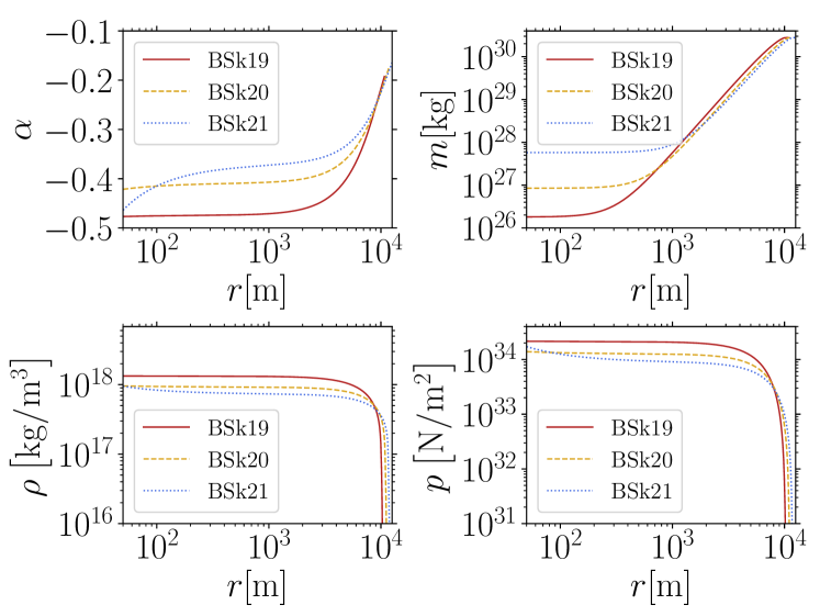
Figure 1: The metric parameter $\alpha(r)$, the mass function $m(r)$, and the density and pressure distributions for different EoS models, BSk19, BSk20, and BSk21.

The accretion of the DM object causes a drag force in the opposite direction of the motion [39, 23],

$$\bm{F}_{\rm AC}=-\dot{m}_{D}\bm{v},$$ (6)

where

$$\dot{m}_{D}=\frac{4\pi\lambda\,\rho\,m_{D}^{2}}{(c_{s}^{2}+v^{2})^{3/2}}$$ (7)

is the accretion rate, an overdot indicates the differentiation with respect to $t$, and $\lambda=0.707$ for the polytropic NS equation of state with the index $\Gamma=4/3$ [18].

Using the quadrupole-octupole formula, the energy loss rate due to GW emissions is written in terms of the multipole moments of the source as

$$\begin{split}\left\langle\frac{dE}{dt}\right\rangle_{\text{GW}}=&-\frac{1}{5}\Big{\langle}\dddot{\mathcal{I}}^{jk}\dddot{\mathcal{I}}^{jk}+\\ &\frac{5}{189}\ddddot{\mathcal{M}}^{jkl}\ddddot{\mathcal{M}}^{jkl}+\frac{16}{9}\dddot{\mathcal{J}}^{jk}\dddot{\mathcal{J}}^{jk}\Big{\rangle},\end{split}$$ (8)

where the overdots indicate the differentiation with respect to the retarded time, $\mathcal{I}^{jk}$, $\mathcal{M}^{jkl}$ and $\mathcal{J}^{jk}$ are the symmetric-traceless parts of mass quadrupole, mass octupole, and flux quadrupole, respectively. For quasi-circular orbits, the energy flux of GW radiation is

$$\begin{split}&\left\langle\frac{dE}{dt}\right\rangle_{\text{GW}}=-\frac{32}{5}r^{4}m_{D}^{2}\Omega^{6}\\ &\quad+\frac{2}{5}r^{4}m_{D}^{2}\Omega^{6}\left[-16r^{2}\Omega^{2}+\left(16+24\delta^{2}\right)U\right]\\ &\quad-\frac{8}{45}r^{6}m_{D}^{2}\Omega^{8}-\frac{2734}{315}r^{6}m_{D}^{2}\Omega^{8}\\ &\quad-\left(\frac{72}{5}r^{4}\Omega^{4}+\frac{4864}{315}r^{6}\Omega^{6}+\frac{8}{5}r^{6}\Omega^{6}\right)\left(\dot{m}_{D}\right)^{2},\end{split}$$ (9)

where $\Omega$ is the orbital angular speed, $U=(1-e^{2\alpha(r)})/2$ and $\delta=e^{2\alpha(r)}-e^{2\beta(r)}$.

With the adiabatic approximation, the DM object follows a geodesic path during each revolution. The energy per unit mass is

$$\hat{E}=\frac{E}{m_{D}}=e^{2\alpha(r)}u^{t},$$ (10)

where

$$u^{t}=\sqrt{\frac{re^{2\beta(r)}f^{r}-1}{r\alpha^{\prime}(r)e^{2\alpha(r)}-e^{2\alpha(r)}}},$$ (11)

$f^{r}$ is the external radial force per unit mass including the dynamical friction force, the drag force, and the radiation reaction force.

For the equatorial circular orbit, the evolution of the orbital radius $r$ is determined by the energy balance condition,

$$\begin{split}\frac{dE}{dt}&=m_{D}\frac{d\hat{E}}{dt}+\dot{m}_{D}\hat{E},\\ &=\left\langle\frac{dE}{dt}\right\rangle_{\text{GW}}+\bm{F}_{\rm DF}\cdot\bm{v}+\bm{F}_{\rm AC}\cdot\bm{v}.\end{split}$$ (12)

Combining Eqs. (5)-(7), (9) and (12), we can obtain the evolution of the orbital radius $r(t)$ and the DM mass $m_{D}(t)$. With $r(t)$, the orbital phase and angular orbital frequency are determined as

$$\begin{split}\Omega(r)=u^{\phi}/u^{t},\\ \varphi(t)=\varphi_{0}+\int_{0}^{t}\Omega(r(t))dt,\end{split}$$ (13)

where $\varphi_{0}$ is the initial orbital phase at $t=0$ and

$$u^{\phi}=\sqrt{\frac{e^{2\alpha(r)}u^{t}u^{t}-1}{r^{2}}}.$$ (14)

The evolution of the orbital radius $r(t)$, the PBH mass $m_{D}(t)$, the orbital phase $\varphi(t)$, and GW frequency $f_{\text{GW}}=\Omega/\pi$ are shown in Fig. 2. From Fig. 2, we see that the evolution timescale is inversely proportional to the PBH mass, and it is shorter for denser NS. As shown in Eqs. (5), (6) and (9), the leading terms of the dynamical friction, accretion, and GW reaction are all proportional to $m_{D}^{2}$, resulting in a shorter evolution timescale for larger PBH mass. The leading terms of the dynamical friction and accretion are both proportional to $\rho$, thus the evolution timescale is shorter for the EoS model related to larger density. For the same mass of PBHs, the orbit of PBH inside BSk19 NS decays the fastest, followed by the orbit in BSk20 NS, and the one in BSk21 NS decays the slowest. Different masses of PBHs and different EoS models lead to different orbital evolution, which will be manifested in the GWs radiated by the system. These frequencies and timescales are consistent with those obtained using a simple analytic density profile $\rho(r)=\rho_{0}\sqrt{1-(r/R)^{2}}$ [24]. As shown in Fig. 2, the orbital radius decreases slowly and the GW frequency is almost constant at the beginning. Then the frequency increases due to the decrease in orbital radius, after that the frequency decreases due to the quick decrease in the mass within $r$.

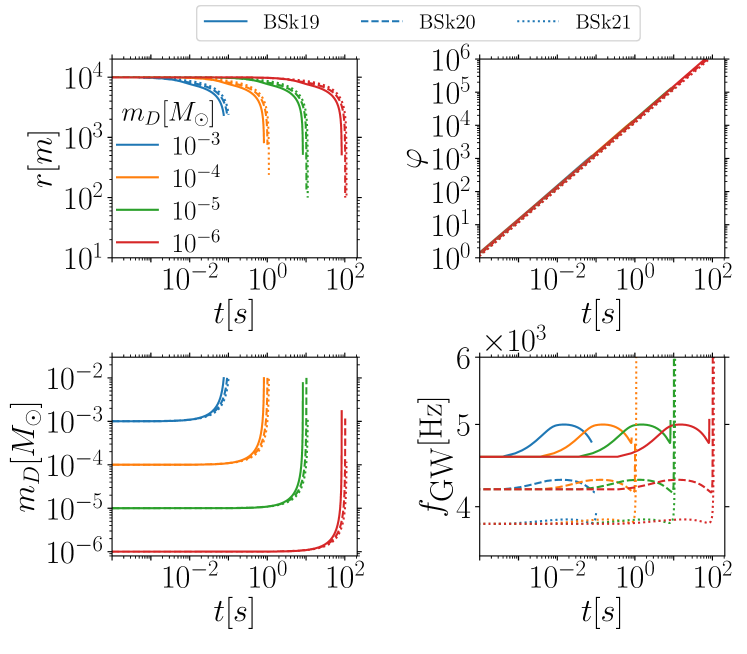
Figure 2: The evolution of the orbital radius $r(t)$, the PBH mass $m_{D}(t)$, the orbital phase $\varphi(t)$ and GW frequency $f_{\rm GW}(t)$ for different EoS models. The initial masses of PBHs are chosen as $10^{-6}$, $10^{-5}$, $10^{-4}$, and $10^{-3}\ M_{\odot}$. The evolution of PBHs begins at $r=10$ km and stops at $r=100$ m or $m_{D}=0.01\ M_{\odot}$.

The GW in the transverse-traceless (TT) gauge is

$$h_{ij}^{\mathrm{TT}}=\frac{2}{d_{L}}\left(P_{il}P_{jm}-\frac{1}{2}P_{ij}P_{lm}\right)\ddot{\mathcal{I}}^{lm},$$ (15)

where $d_{L}$ is the luminosity distance to the source, $P_{ij}=\delta_{ij}-n_{i}n_{j}$ is the projection operator acting onto GWs with the unit propagating direction $n_{j}$. The GW strain measured by the detector is

$$h(t)=h_{+}(t)F^{+}(t)+h_{\times}(t)F^{\times}(t),$$ (16)

where $h_{+,\times}$ are the two GW polarizations given by [40, 41]

$$\begin{split}h_{+}(t)=&\frac{4r(t)^{2}}{d_{L}}\frac{1+\cos^{2}\iota}{2}\bigg{[}\Omega(r(t))^{2}\cos\left(2\varphi(t)\right)\\ &+\Omega(r(t))\sin\left(2\varphi(t)\right)\dot{m}_{D}\bigg{]},\\ h_{\times}(t)=&-\frac{4r(t)^{2}}{d_{L}}\cos\iota\bigg{[}\Omega(r(t))^{2}\sin\left(2\varphi(t)\right)\\ &-\Omega(r(t))\cos\left(2\varphi(t)\right)\dot{m}_{D}\bigg{]},\end{split}$$ (17)

$\iota$ is the inclination angle between the binary orbital angular momentum and the line of sight, $F^{+,\times}(t)$ are the interferometer pattern functions. The amplitudes of GWs from PBHs inside NSs are shown in Fig. 3. From Fig. 3, we see that the amplitudes of GWs are nearly constant and proportional to the PBH masses. The amplitudes are larger for the EoS model with a larger density.

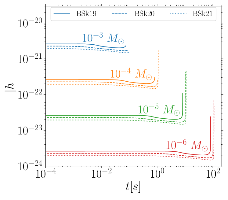
Figure 3: Amplitudes of GWs from PBHs inside NSs for different EoS models. The initial masses of PBHs are chosen as $10^{-6}$, $10^{-5}$, $10^{-4}$, and $10^{-3}\ M_{\odot}$. The GW strain is $h=h_{+}-ih_{\times}$, the inclination angle $\iota=\pi/3$, and $d_{L}=10\ \text{kpc}$. The evolution of PBHs starts at $r=10$ km, and ends at $r=100$ m or $m_{D}=0.01\ M_{\odot}$.

The faithfulness between two signals is defined as

$$\mathcal{F}_{n}[h_{1},h_{2}]=\max_{\{t_{0},\phi_{0}\}}\frac{\langle h_{1}|h_{2}\rangle}{\sqrt{\langle h_{1}|h_{1}\rangle\langle h_{2}|h_{2}\rangle}}\ ,$$ (18)

where $(t_{0},\phi_{0})$ are time and phase offsets [42], the noise-weighted inner product between two templates $h_{1}$ and $h_{2}$ is

$$\left\langle h_{1}|h_{2}\right\rangle=4\Re\int_{f_{\min}}^{f_{\max}}\frac{\tilde{h}_{1}(f)\tilde{h}_{2}^{*}(f)}{S_{n}(f)}df,$$ (19)

$\tilde{h}_{1}(f)$ is the Fourier transform of the time-domain signal $h_{1}(t)$, its complex conjugate is $\tilde{h}_{1}^{*}(f)$, and $S_{n}(f)$ is the noise spectral density for the GW detector, here we chose the noise spectral density of ET as an example [43]. The signal-to-noise ratio (SNR) is given by

$$\text{SNR}=\left\langle h|h\right\rangle^{1/2}.$$ (20)

Table 1 shows the faithfulness between GWs using different EoS models. The faithfulness is smaller for the PBH with a larger mass and shorter evolution timescale. Since two signals are distinguishable by the detector if the faithfulness $\mathcal{F}_{n}<1-5/\rm{SNR}^{2}$ [44, 42, 45, 46], the results in Table 1 tell us that we can use GWs from PBHs inspiralling inside NSs within the Milky Way galaxy detected by ET to distinguish EoS models BSk19, BSk20, and BSk21.

$m_{D}[M_{\odot}]$	BSk19-BSk20	BSk19-BSk21	BSk20-BSk21	$\rm{SNR}$
$10^{-3}$	0.0318	0.0385	0.1353	126/89/81
$10^{-4}$	0.0007	0.0016	0.0033	42/29/26
$10^{-5}$	0.0003	0.0004	0.0009	13/9/8
$10^{-6}$	0.00002	0.00002	0.00005	4/3/3

Table 1: The faithfulness between GWs from PBHs with different initial masses inspiralling inside NSs with different EoS models detected by ET. We only use GW signals from PBHs evolving from $r=10$ km to $r=1$ km. The three values of SNR on the same row are related to EoS models BSk19, BSk20, and BSk21, respectively.

Measuring the EoS of NSs will be possible with next-generation gravitational wave detectors. The event where a PBH is captured by an NS serves as a proof of concept for distinguishing EoS models, such as BSk19, BSk20, and BSk21. We generate more accurate GW templates by providing the interior metric of NSs and including more realistic effects of the dynamical friction, accretion, and quadrupole-octupole GW reaction during the PBH’s evolution. We also use the faithfulness between GWs from PBHs with masses $\left\{10^{-3},10^{-4},10^{-5},10^{-6}\right\}\ M_{\odot}$ captured by NSs described by EoS models BSk19, BSk20, and BSk21 to distinguish different EoS models. We conclude that ET can use GWs from PBHs inspiralling inside NSs within the Milky Way galaxy to distinguish EoS models BSk19, BSk20, and BSk21. The result is helpful for understanding the physics of NSs.