A novel class of explicit energy-preserving splitting methods for charged-particle dynamics

Abstract

In this letter, based on the exponential scalar auxiliary variable technology, we propose and study a new class of explicit energy-preserving splitting methods for solving the charged-particle dynamics. The energy-preserving property of these methods is rigorously analysed. We also provide the error estimates for the new methods. Numerical computations are presented, which confirm the effectiveness and superiority of these novel methods in comparison with the standard scalar auxiliary variable approach.

Mathematics Subject Classification (2010): 65L05, 78A35, 78M25

1 Introduction

In this letter, we focus on the charged-particle dynamics (CPD) [2, 3]

$$\begin{split}&\ddot{x}(t)=\dot{x}(t)\times B(x(t))+E(x(t)),\ \ x(0)=x^{0},\ \dot{x}(0)=\dot{x}^{0},\ t\in[0,T],\end{split}$$ (1)

with the position $x(t)\in\mathbb{R}^{3}$ and the velocity $v(t):=\dot{x}(t)\in\mathbb{R}^{3}$ of a particle. The particle, whose initial values are $x^{0}$ and $v^{0}:=\dot{x}^{0}\in\mathbb{R}^{3}$, is moving in an non-uniform magnetic field $B(x(t))=(b_{1}(x),b_{2}(x),b_{3}(x))^{\intercal}$ and an electric field $E(x)=-\nabla_{x}U(x)$ with some scalar potential $U(x)$. The total energy of the CPD is conserved along the solution of (1) and it is in the form of

$$H\left(x(t),v(t)\right)=\frac{1}{2}\left|v(t)\right|^{2}+U(x(t)),\quad t\geq 0,$$ (2)

with the Euclidean norm $\left|\cdot\right|$.

In recent years, the energy-preserving (EP) property of numerical methods for solving CPD has gained considerable attention, and numerous EP methods ([4, 5, 6, 7, 8, 9, 10]) have been constructed and analysed to solve this system. However, all these methods are implicit and a nonlinear iteration is needed in practical computations. Thus it is time-consuming to adopt them to calculate the CPD in comparison with explicit methods. In order to improve the computational efficiency of EP methods, the sacalar auxiliary variable (SAV) [11, 12, 13] approach has been considered to formulate a class of linearly implicit splitting EP schemes (see e.g. in [14]) which are shown to be more efficient. By introducing an auxiliary scalar, the SAV approach is proposed for constructing energy stable schemes for a broad class of gradient flows [15, 16] and has been effectively used in a number of conservative systems, such as Hamiltonian systems [17, 18]. The standard SAV approach for the system (1) is formulated under the condition that the scalar potential $U(x)$ is bounded from below, i.e., there exists a positive constant $c_{0}$ such that $U(x)\geq-c_{0}$. Then we can introduce a scalar $s(t)=\sqrt{U(x)+C_{0}}$ ($C_{0}>c_{0}$) and apply splitting technology to obtain numerical schemes (see [14]). For example, using SAV approach, the first-order scheme (denoted by S1-SAV) has been derived in [14], which reads

$$x^{n+1}=x^{n}+he^{h\tilde{B}(x^{n})}v^{n}+\frac{h^{2}}{2}\frac{E(\hat{x}^{n+\frac{1}{2}})}{\sqrt{U(\hat{x}^{n+\frac{1}{2}})+C_{0}}}s^{n+\frac{1}{2}},\ \ v^{n+1}=e^{h\tilde{B}(x^{n})}v^{n}+h\frac{E(\hat{x}^{n+\frac{1}{2}})}{\sqrt{U(\hat{x}^{n+\frac{1}{2}})+C_{0}}}s^{n+\frac{1}{2}},$$ (3)

$$s^{n+1}=s^{n}-\frac{(x^{n+1}-x^{n})^{\intercal}E(\hat{x}^{n+\frac{1}{2}})}{2\sqrt{U(\hat{x}^{n+\frac{1}{2}})+C_{0}}},$$

with the approximate term $\hat{x}^{n+\frac{1}{2}}=x^{n}+\frac{h}{2}e^{h\tilde{B}(x^{n})}v^{n}$ and the notation $s^{n+\frac{1}{2}}=\frac{s^{n+1}+s^{n}}{2}$, where $h$ is the time stepsize. According to the analysis in [14], we know that the S1-SAV exactly preserves the modified energy $\tilde{H}(v,s)=\frac{1}{2}\left|v\right|^{2}+s^{2}-C_{0}$ at the discrete level. In addition, for the schemes presented in [14], there are three aspects that can be improved.

• The lower bound condition is required for the scalar potential $U(x)$, which is not always satisfied, such as the case that $U(x)=x_{1}^{3}-x_{2}^{3}+x_{1}^{4}/5+x_{2}^{4}+x_{3}^{4}$.

• In the implementation of the methods of [14], since the scheme is linearly implicit, the calculation of solution variables and the auxiliary variable can not be decoupled. Thus we have to determine the inner product $\left(E(\hat{x}^{n+\frac{1}{2}})\right)^{\intercal}x^{n+1}$ before computing $x^{n+1}$, which would become more complicated for high-order SAV schemes.

• It is obvious that the scalar $s(t)>0$. However it is difficult to guarantee that its numerical solution presented in (3) also satisfies $s^{n}>0$.

Motivated by these points, we propose and study a new kind of explicit energy-preserving splitting methods for charged-particle dynamics. The new methods do not need the lower bound condition of $U(x)$ and are completely explicit which makes the methods can be implemented more efficiently. Moreover, the new methods can share the property $s(t)>0$ of the scalar $s(t)$. The proposed methods are formulated based on the exponential scalar auxiliary variable (E-SAV) technology which was firstly presented in [19] and has been popular in the formulation of effective methods for various phase field models such as Hamiltonian PDEs [20] and Allen-Cahn type equations [21]. For the system of CPD, using its specific structure and the E-SAV technology, we can get rid of the assumption of the nonlinear potential scalar in the SAV approach, and this yields totally explicit energy stable schemes. As a result, we obtain a decoupled scheme, and the time consumption of E-SAV is more efficient than SAV.

The rest of this letter is organized as follows. By introducing an exponential scalar auxiliary, Section 2 presents two explicit splitting methods and analyzes their energy-preserving properties and global error bounds. In Section 3, a numerical experiment is given to demonstrate the energy, cputime and accuracy behaviour of the obtained methods in comparison with the method S1-SAV. Section 4 includes the conclusion of this letter.

2 Numerical methods and their properties

In this section, we first consider an exponential scalar auxiliary variable: $r(t)=\exp(U(x))$. Then the equation (1) can be transformed into

$$\frac{d}{dt}\begin{pmatrix}x\\ v\\ r\end{pmatrix}=\begin{pmatrix}v\\ \tilde{B}(x)v+\frac{E(x)}{\exp(U(x))}r\\ -\exp(U(x))\dot{x}^{\intercal}E(x)\end{pmatrix}\ \ \textmd{with}\ \ \tilde{B}(x)=\begin{pmatrix}0&b_{3}(x)&-b_{2}(x)\\ -b_{3}(x)&0&b_{1}(x)\\ b_{2}(x)&-b_{1}(x)&0\end{pmatrix}.$$

Now we reformulate the above equation as

$$\frac{d}{dt}\begin{pmatrix}x\\ v\\ \ln(r)\end{pmatrix}=\begin{pmatrix}v\\ \tilde{B}(x)v+\frac{E(x)}{\exp(U(x))}r\\ -\frac{\dot{x}^{\intercal}E(x)}{\exp(U(x))}r\end{pmatrix},\quad\begin{pmatrix}x(0)\\ v(0)\\ \ln(r(0))\end{pmatrix}={\begin{pmatrix}x^{0}\\ v^{0}\\ \ln(r^{0})\end{pmatrix}},$$ (4)

where $v^{0}:=\dot{x}^{0}$ and $r^{0}:=\exp(U(x^{0}))$. In order to obtain the numerical solution of the system (4), we split it into two subflows:

$$\frac{d}{dt}\begin{pmatrix}x\\ v\\ \ln(r)\end{pmatrix}=\begin{pmatrix}0\\ \tilde{B}(x)v\\ 0\end{pmatrix},\quad\frac{d}{dt}\begin{pmatrix}x\\ v\\ \ln(r)\end{pmatrix}=\begin{pmatrix}v\\ \frac{E(x)}{\exp(U(x))}r\\ -\frac{\dot{x}^{\intercal}E(x)}{\exp(U(x))}r\end{pmatrix}.$$ (5)

For the first subflow, which is linear, it is easy to get its exact solution $\Phi_{t}^{L}$: $\begin{pmatrix}x(t)\\ v(t)\\ \ln(r(t))\end{pmatrix}=\begin{pmatrix}x(0)\\ e^{\tilde{B}(x(0))}v(0)\\ \ln(r(0))\end{pmatrix}.$ Subsequently, for the second subflow of (5), we denote $F(x,r):=\frac{E(x)}{\exp(U(x))}r$ and consider the following explicit numerical propagator $\Phi_{h}^{NL}$:

$$x^{n+1}=x^{n}+hv^{n}+\frac{h^{2}}{2}{F(\tilde{x}^{n+\frac{1}{2}},\tilde{r}^{n+\frac{1}{2}})},\ \ v^{n+1}=v^{n}+h{F(\tilde{x}^{n+\frac{1}{2}},\tilde{r}^{n+\frac{1}{2}})},\ \ln(r^{n+1})=\ln(r^{n})-(x^{n+1}-x^{n})^{\intercal}{F(\tilde{x}^{n+\frac{1}{2}},\tilde{r}^{n+\frac{1}{2}})},$$ (6)

where $h$ is the time stepsize, $\tilde{x}^{n+\frac{1}{2}}=x^{n}+\frac{h}{2}v^{n}$ and $\tilde{r}^{n+\frac{1}{2}}=r^{n}-\frac{h}{2}\exp(U(\tilde{x}^{n+\frac{1}{2}}))(v^{n})^{\intercal}E(\tilde{x}^{n+\frac{1}{2}})$ are respectively numerical approximations for $x(t_{n+\frac{1}{2}})$ and $r(t_{n+\frac{1}{2}})$ with the accuracy $\mathcal{O}(h^{2})$ and $t_{n+\frac{1}{2}}=\big{(}n+\frac{1}{2}\big{)}h$. Finally, we can obtain $r^{n+1}=\exp\left[\ln(r^{n})-(x^{n+1}-x^{n})^{\intercal}{F(\tilde{x}^{n+\frac{1}{2}},\tilde{r}^{n+\frac{1}{2}})}\right].$

With the above preparations, we are now in the position to present the scheme of the explicit energy-preserving splitting methods.

Algorithm 2.1

(Explicit Energy-Preserving Splitting Methods) For the sake of brevity, we denote the numerical solution as $x^{n}\approx x(t_{n})$, $v^{n}\approx v(t_{n})$. On the basis of the composition of $\Phi_{h}^{L}$ and $\Phi_{h}^{NL}$, we derive the following explicit schemes, such as the first order splitting scheme $\Phi_{h}^{1}=\Phi_{h}^{NL}\circ\Phi_{h}^{L}$ (S1-ESAV):

$$x^{n+1}=x^{n}+he^{h\tilde{B}(x^{n})}v^{n}+\frac{h^{2}}{2}{F(\hat{x}^{n+\frac{1}{2}},\hat{r}^{n+\frac{1}{2}})},\ \ v^{n+1}=e^{h\tilde{B}(x^{n})}v^{n}+h{F(\hat{x}^{n+\frac{1}{2}},\hat{r}^{n+\frac{1}{2}})},$$ (7)

$$\ln(r^{n+1})=\ln(r^{n})-(x^{n+1}-x^{n})^{\intercal}{F(\hat{x}^{n+\frac{1}{2}},\hat{r}^{n+\frac{1}{2}})},$$

with the approximate terms $\hat{x}^{n+\frac{1}{2}}=x^{n}+\frac{h}{2}e^{h\tilde{B}(x^{n})}v^{n}$, $\hat{r}^{n+\frac{1}{2}}=r^{n}-\frac{h}{2}\exp(U(\hat{x}^{n+\frac{1}{2}}))\left(e^{h\tilde{B}(x^{n})}v^{n}\right)^{\intercal}E(\hat{x}^{n+\frac{1}{2}})$ and the second order Strang splitting scheme $\Phi_{h}^{2}=\Phi_{h/2}^{L}\circ\Phi_{h}^{NL}\circ\Phi_{h/2}^{L}$ (S2-ESAV):

$$x^{n+1}=x^{n}+he^{\frac{h}{2}\tilde{B}(x^{n})}v^{n}+\frac{h^{2}}{2}{F(\widehat{x}^{n+\frac{1}{2}},\widehat{r}^{n+\frac{1}{2}})},\ \ v^{n+1}=e^{\frac{h}{2}\tilde{B}(x^{n+1})}\left[e^{\frac{h}{2}\tilde{B}(x^{n})}v^{n}+h{F(\widehat{x}^{n+\frac{1}{2}},\widehat{r}^{n+\frac{1}{2}})}\right],$$ (8)

$$\ln(r^{n+1})=\ln(r^{n})-(x^{n+1}-x^{n})^{\intercal}{F(\widehat{x}^{n+\frac{1}{2}},\widehat{r}^{n+\frac{1}{2}})},$$

with the approximate terms $\widehat{x}^{n+\frac{1}{2}}=x^{n}+\frac{h}{2}e^{\frac{h}{2}\tilde{B}(x^{n})}v^{n}$ and $\widehat{r}^{n+\frac{1}{2}}=r^{n}-\frac{h}{2}\exp(U(\widehat{x}^{n+\frac{1}{2}}))\left(e^{\frac{h}{2}\tilde{B}(x^{n})}v^{n}\right)^{\intercal}E(\widehat{x}^{n+\frac{1}{2}})$. These two methods are denoted by SESAVs.

It is noted that higher-order schemes can be produced by applying the Triple Jump splitting to S2-ESAV, but we skip this in the letter for brevity. In what follows, we study the energy-preserving property of these two splitting schemes.

Theorem 2.2

(Energy-Preserving property) The two splitting schemes formulated in Algorithm 2.1 exactly preserve the energy $H(x^{0},v^{0})$ of the CPD (1).

Proof.   To this end, we first prove that the second subflow of (5) exactly conserves the modified energy $\hat{H}$ with the scheme

$$\hat{H}(v,r):=\frac{1}{2}\left|v\right|^{2}+\ln(r)=H(x,v).$$ (9)

For the second subflow, taking the inner product with $v$ of the second equality and using the other two equalities, it is obtained that

$${\frac{d}{dt}\left(\frac{1}{2}\left|v\right|^{2}+\ln(r)\right)=v^{\intercal}\dot{v}+\frac{\dot{r}}{r}=v^{\intercal}\frac{E(x)}{\exp(U(x))}r-\frac{\dot{x}^{\intercal}E(x)}{\exp(U(x))}r=0},$$

which shows that $\frac{d}{dt}\hat{H}(v,r)=0$ and further yields (9).

Then we prove that the two schemes preserve the modified energy (9) at the discrete level, i.e.,

$$\hat{H}(v^{n+1},r^{n+1})=\hat{H}(v^{n},r^{n}),\ \ \text{for}\ \ n=0,1,2,\dots,T/h-1.$$ (10)

It can be deduced from $v^{n+1}$ and $\ln(r^{n+1})$ in (7) that

$$\frac{1}{2}\left|v^{n+1}\right|^{2} =\frac{1}{2}\left[e^{h\tilde{B}(x^{n})}v^{n}+h{F(\hat{x}^{n+\frac{1}{2}},\hat{r}^{n+\frac{1}{2}})}\right]^{\intercal}\left[e^{h\tilde{B}(x^{n})}v^{n}+h{F(\hat{x}^{n+\frac{1}{2}},\hat{r}^{n+\frac{1}{2}})}\right]$$

$$=\frac{1}{2}\left|v^{n}\right|^{2}+\left[he^{h\tilde{B}(x^{n})}v^{n}+\frac{h^{2}}{2}{F(\hat{x}^{n+\frac{1}{2}},\hat{r}^{n+\frac{1}{2}})}\right]^{\intercal}{F(\hat{x}^{n+\frac{1}{2}},\hat{r}^{n+\frac{1}{2}})}$$

$$=\frac{1}{2}\left|v^{n}\right|^{2}-\ln(r^{n+1})+\ln(r^{n}),$$

which indicates that (10) holds for S1-ESAV. It is clear that the modified energy-preserving property (10) of S2-ESAV can be proved in the same way.

Finally, based on the above proof and noting $\hat{H}(v,r)=H(x,v)$, it is immediately concluded that our two methods satisfy

$$\hat{H}(v^{n},r^{n})=\hat{H}(v^{0},r^{0})=H(x^{0},v^{0})\ \ \text{for}\ \ n=1,2,\dots,T/h,$$ (11)

which completes the proof. $\blacksquare$

It should be pointed out that the numerical results $r^{n}$ and $x^{n}$ produced by Algorithm 2.1 usually do not satisfy $r^{n}=\exp(U(x^{n}))$. Thus the statement (9) does not hold anymore for Algorithm 2.1, i.e., $\hat{H}(v^{n},r^{n})\neq H(x^{n},v^{n})$. That’s the reason why we prove the result (11) in Theorem 2.2 instead of $H(x^{n},v^{n})=H(x^{0},v^{0})$.

Theorem 2.3

(Global errors) Supposing that the nonlinear function $E(x):\mathbb{R}^{3}\rightarrow\mathbb{R}^{3}$ is sufficiently smooth, there exists a sufficient small $0<\alpha\leq 1$, such that when $0<h\leq\alpha$, we have

$$\textmd{S1-ESAV:}\qquad x^{n+1}-x(t_{n+1})=\mathcal{O}(h),\ \ x^{n+1}-x(t_{n+1})=\mathcal{O}(h),$$

$$\textmd{S2-ESAV:}\qquad x^{n+1}-x(t_{n+1})=\mathcal{O}(h^{2}),\ \ x^{n+1}-x(t_{n+1})=\mathcal{O}(h^{2}),$$

where $n=0,1,2,\dots,T/h-1$ and the constants symbolized by $\mathcal{O}$ can depend on $T$ but not on $n,h$.

Proof.   The proof is based on Taylor expansion and the local error analysis of splitting, which is omitted here for brevity. $\blacksquare$

Besides the above results, there are some points which need to be noted.

Remark 2.4

From the scheme of the two methods, it follows that the methods keep the same property $r^{n+1}>0$ as the exact solution $r(t)>0$. It is also remarked that the proposed methods are explicit, and therefore they are more efficient than linearly implicit methods in practical computations.

Remark 2.5

It is worth mentioning that the exponential function is rapidly increasing and thus there may exist a rapidly increase of errors which may lead Algorithm 2.1 to lose efficiency. In order to avoid this point, we add a suitable positive constant $C=\left|H(x^{0},v^{0})\right|$ in the exponential scalar auxiliary variable: $r(t)=\exp\left(\frac{U(x)}{C}\right)$ and define $G(x,r):=\frac{E(x)}{\exp(U(x)/C)}r$, then we can obtain the modified S1-ESAV (S1-MESAV) in the form:

$$x^{n+1}=x^{n}+he^{h\tilde{B}(x^{n})}v^{n}+\frac{h^{2}}{2}{G(\hat{x}^{n+\frac{1}{2}},\hat{r}^{n+\frac{1}{2}})},\ \ v^{n+1}=e^{h\tilde{B}(x^{n})}v^{n}+h{G(\hat{x}^{n+\frac{1}{2}},\hat{r}^{n+\frac{1}{2}})},$$ (12)

$$\ln(r^{n+1})=\ln(r^{n})-\frac{(x^{n+1}-x^{n})^{\intercal}}{C}{G(\hat{x}^{n+\frac{1}{2}},\hat{r}^{n+\frac{1}{2}})}.$$

In a same way, we can get the expression of modified S2-ESAV (S2-MESAV) and the above two modified methods are referred as SMESAVs. With the same arguments as above, it can be shown that these two modified methods preserve the modified energy $\widehat{H}(v,r)=\frac{1}{2}\left|v\right|^{2}+C\ln(r)$.

3 Numerical experiment

In Section 2, a novel class of explicit energy-preserving splitting schemes SESAVs and SMESAVs were proposed for CPD. To demonstrate their numerical behaviour in accuracy, cputime, and energy conservation, we present a numerical experiment in this section. The linearly implicit splitting method S1-SAV (3) is used to make a comparison with SESAVs. The “ode45” function of MATLAB is used to get the reference solution.

We consider the lower bound case of $U$ where the scalar potential is chosen as $U(x)=\frac{1}{100\sqrt{x_{1}^{2}+x_{2}^{2}}}$ to compare with S1-SAV and the magnetic field is chosen as ([3]): $B(x)={\frac{1}{\varepsilon}}(0,0,\sqrt{x_{1}^{2}+x_{2}^{2}})^{\intercal}.$ For initial values we take $x(0)=(0,1,0.1)^{\intercal}$ and $v(0)=(0.09,0.05,0.2)^{\intercal}$. Figure 1 shows the relative energy errors: $e\tilde{H}:=\frac{\left|\tilde{H}(x^{n},r^{n})-H(x^{0},v^{0})\right|}{\left|H(x^{0},v^{0})\right|}$ with the scalar $r=\sqrt{U(x)+1}$ and the modified energy $\tilde{H}(v,r)=\frac{1}{2}\left|v\right|^{2}+r^{2}-1$ for S1-SAV, $e\hat{H}:=\frac{\left|\hat{H}(x^{n},r^{n})-H(x^{0},v^{0})\right|}{\left|H(x^{0},v^{0})\right|}$ with the scalar $r=\exp(U(x))$ and the modified energy $\hat{H}(v,r)=\frac{1}{2}\left|v\right|^{2}+\ln(r)$ for SESAVs, and $e\widehat{H}:=\frac{\left|\widehat{H}(x^{n},r^{n})-H(x^{0},v^{0})\right|}{\left|H(x^{0},v^{0})\right|}$ with the scalar $r=\exp(U(x)/C)$, the constant $C=\left|H(x^{0},v^{0})\right|$ and the modified energy $\widehat{H}(v,r)=\frac{1}{2}\left|v\right|^{2}+C\ln(r)$ for SMESAVs. The global errors $error:=\frac{\left|x^{n}-x(t_{n})\right|}{\left|x(t_{n})\right|}+\frac{\left|v^{n}-v(t_{n})\right|}{\left|v(t_{n})\right|}$ are displayed in Figure 2. Furthermore, Figure 3 presents the cputime of S1-SAV and S1-ESAV.

The following observations can be drawn from Figures 1-3. a) SESAVs and SMESAVs are energy-preserving, and the later ones hold a better energy behavior than the former especially in the case $\varepsilon=1$. b) S1-ESAV behaves a same precision as S1-SAV but has a better energy-preserving property. c) Figure 3 illustrates that S1-ESAV outperforms S1-SAV in terms of computing efficiency. In this numerical example, the performances of accuracy and cputime of SESAVs and SMESAVs are similar, and so we omit them for brevity.

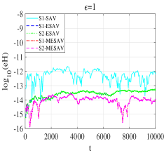
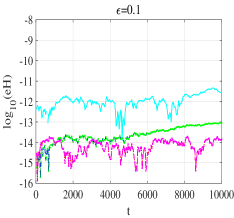
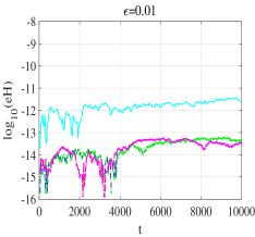
Figure 1: Evolution of the energy error $e_{H}$ as function of time $t$.

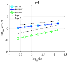
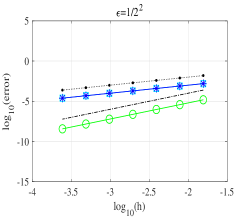
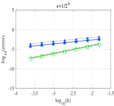
Figure 2: The global errors $error$ with $t=1$ and $h=1/2^{k}$ for $k=6,\ldots,12$ under different $\varepsilon$.

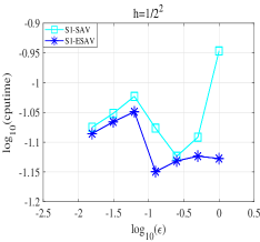
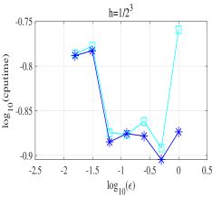
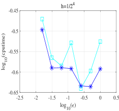
Figure 3: The cputime with $T=100$ and $\varepsilon=1/2^{k}$ for $k=0,1,\ldots,6$ under different $h$.

4 Conclusion

In this letter, we have proposed two energy-preserving splitting methods (SESAVs) for the charged-particle dynamics. It was shown that these SESAVs are explicit and exactly preserve the energy of the charged-particle dynamics. The accuracy of SESAVs was also presented. A numerical experiment was carried out to illustrate the accuracy and energy conservation of these methods.

References

• [1]
• [2] W.W. Lee, Gyrokinetic approach in particle simulation, Phys. Fluids. 26 (1983) 556-562.
• [3] E. Hairer, C. Lubich, Long-term analysis of a variational integrator for charged-particle dynamics in a strong magnetic field, Numer. Math. 144 (2020) 699-728.
• [4] L. Brugnano, F. Iavernaro, R. Zhang, Arbitrarily high-order energy-preserving methods for simulating the gyrocenter dynamics of charged particles, J. Comput. Appl. Math., 380 (2020) 112994.
• [5] L. Brugnano, J.I. Montijano, L. Rándz, High-order energy-conserving line integral methods for charged particle dynamics, J. Comput. Phys. 396 (2019) 209-227.
• [6] T. Li, B. Wang, Arbitrary-order energy-preserving methods for charged-particle dynamics, Appl. Math. Lett. 100 (2020) 106050.
• [7] L. F. Ricketson, L. Chacón, An energy-conserving and asymptotic-preserving charged-particle orbit implicit time integrator for arbitrary electromagnetic fields, J. Comput. Phys. 418 (2020) 109639.
• [8] B. Wang, X. Zhao, Error estimates of some splitting schemes for charged-particle dynamics under strong magnetic field. SIAM J. Numer. Anal. 59 (2021) 2075-2105.
• [9] X. Li, B. Wang, Energy-preserving splitting methods for charged-particle dynamics in a normal or strong magnetic field, Appl. Math. Lett. 124 (2022) 107682.
• [10] B. Wang, Exponential energy-preserving methods for charged-particle dynamics in a strong and constant magnetic field, J. Comput. Appl. Math. 387 (2021) 112617.
• [11] J. Shen, J. Xu, J. Yang, The scalar auxiliary variable (SAV) approach for gradient, J. Comput. Phys. 353 (2018) 407-416.
• [12] J. Shen, J. Xu, J. Yang, A new class of efficient and robust energy stable schemes for gradient flows, SIAM Rev. 61(2019) 474-506.
• [13] X. Li, J. Shen, H. Rui, Energy stability and convergence of SAV block-centered finite difference method for gradient flows, Math. Comp. 88 (2019) 2047-2068.
• [14] X. Li, B. Wang, A novel class of linearly implicit energy-preserving schemes for conservative systems, arXiv.2302.07472.
• [15] S. M. Allen, J. W. Cahn, A microscopic theory for antiphase boundary motion and its application to antiphase domain coarsening, Acta Metallurgica. 27 (1979) 1085-1095.
• [16] J. W. Cahn, J. E. Hilliard, Free energy of a nonuniform system, I. Interfacial free energy, J. Chem. Phys. 28 (1958) 258-267.
• [17] W. Cai, C. Jiang, Y. Wang, Y. Song. Structure-preserving algorithms for the two-dimensional sine-Gordon equation with Neumann boundary conditions. J. Comput. Phys. 395 (2019) 166-185.
• [18] J. Cai, J. Shen, Two classes of linearly implicit local energy-preserving approach for general multi-symplectic Hamiltonian PDEs. J. Comput. Phys. 401 (2020) 108975.
• [19] Z. Liu, X. Li, The exponential scalar auxiliary variable (E-SAV) approach for phase field models and its explicit computing, SIAM J. Sci. Comput. 42 (2020) B630-B655.
• [20] Y. Bo, Y. Wang, W. Cai, Arbitrary high-order linearly implicit energy-preserving algorithms for Hamiltonian PDEs. Numer. Algor. 90 (2022) 1519–1546.
• [21] L. Ju, X. Li, Z. Qiao, Stabilized exponential-SAV schemes preserving energy dissipation law and maximum bound principle for the Allen–Cahn type equations, J. Sci. Comput. 92 (2022) 66.
• [22] E. Hairer, C. Lubich, G. Wanner, Geometric Numerical Integration: Structure-Preserving Algorithms for Ordinary Differential Equations, 2nd edn. Springer-Verlag, Berlin, Heidelberg, (2006).