Personalized Graph Federated Learning with Differential Privacy

Abstract

This paper presents a personalized graph federated learning (PGFL) framework in which distributedly connected servers and their respective edge devices collaboratively learn device or cluster-specific models while maintaining the privacy of every individual device. The proposed approach exploits similarities among different models to provide a more relevant experience for each device, even in situations with diverse data distributions and disproportionate datasets. Furthermore, to ensure a secure and efficient approach to collaborative personalized learning, we study a variant of the PGFL implementation that utilizes differential privacy, specifically zero-concentrated differential privacy, where a noise sequence perturbs model exchanges. Our mathematical analysis shows that the proposed privacy-preserving PGFL algorithm converges to the optimal cluster-specific solution for each cluster in linear time. It also shows that exploiting similarities among clusters leads to an alternative output whose distance to the original solution is bounded, and that this bound can be adjusted by modifying the algorithm’s hyperparameters. Further, our analysis shows that the algorithm ensures local differential privacy for all clients in terms of zero-concentrated differential privacy. Finally, the performance of the proposed PGFL algorithm is examined by performing numerical experiments in the context of regression and classification using synthetic data and the MNIST dataset.

I Introduction

The rise of internet-of-things (IoT) and cyber-physical systems has led to exponential growth in data collection from distributed devices. However, transferring this massive amount of data to a centralized processing point for inference and decision-making is often impractical due to resource constraints and privacy concerns. To overcome these challenges, distributed learning, with its on-device processing, is an attractive alternative, enabling efficient data analysis without moving the raw data out of the edge devices. Federated learning (FL) is a distributed learning framework that facilitates collaborative model training across edge devices or clients without exposing the underlying data [2, 3, 4]. In particular, using its local data, each client refines a global model shared by a server, and subsequently transfers the updated model back to the server which then aggregates all updated client models before sending an update back to clients for further refinements.

To date, research on FL mostly uses a single-server architecture, which is susceptible to communication and computation bottlenecks and scales poorly with the number and geographical dispersion of participating clients. To address these concerns, some alternatives to the single-server architecture have been proposed, see, e.g., [5, 6, 7, 8], such as client-edge-server hierarchical learning [6] and the graph federated architecture [5, 8]. In client-edge-server hierarchical learning, edge servers perform partial aggregation with their associated clients and communicate their results to a single cloud server that performs the global aggregation. However, using a single cloud server is susceptible to bottlenecks and can only accommodate up to a limited number of edge servers. In contrast, the graph federated architecture uses a server network in which each server aggregates the information from its associated clients and shares its model with its neighbors. Therefore, the graph federated architecture is highly scalable with the number of clients and easier to implement, thanks to its distributed nature.

One of the main challenges in FL is data heterogeneity, which means there can be substantial differences in the underlying statistical distributions among clients’ data [9, 10, 11]. Consequently, a unique globally shared model can be inadequate for such settings, and personalized models must be learned instead [12, 13, 14]. For example, autonomous vehicles need to maintain vehicle-specific models of their highly dynamic environment while collaborating with nearby vehicles and/or smart city IoT devices [10]. This requirement can be met by personalized FL, where clients, or groups of clients (clusters), learn client- or cluster-specific models [15, 16, 17]. These personalized models typically share some similarities [18]. As an example, the environment of an autonomous vehicle could be shared with other connected objects. Leveraging the similarities between cluster-specific models can, therefore, improve performance [18, 19], a process known as inter-cluster learning, which is particularly important when some clients or clusters have insufficient data [20, 21].

Personalized FL has received considerable attention lately due to its ability to improve learning performance in settings where clients are required to observe device-specific behaviors, see, e.g., [18, 22, 23, 24, 20, 21]. It is used in many applications such as healthcare, electrical load forecasting, biometrics, drone swarms, and autonomous vehicles [11, 25, 26, 27, 10]. However, all those works are limited to single-server cases. For example, although [8] extends personalized FL to a multi-server architecture, it assumes that all the clients associated with a given server learn the same model. Under this assumption, each server maintains a single model trained via conventional FL and the model is refined by communicating with other servers about their models. However, the general case where each distributed server needs to enable the learning of personalized models and collaborate with its neighbors to refine those, is yet to be studied.

In the context of graph FL, many devices take part in the training process, and ensuring the privacy and security of client data is crucial. The risk of eavesdropping attacks on the client-server channels increases with the number of devices in the system, and not all devices can be trusted. Even if data is not explicitly shared among clients, repeated message exchanges could reveal sensitive information to curious devices or external eavesdroppers [28, 29]. In order to reduce this risk, differential privacy (DP) has been introduced to protect client privacy by ensuring that the inclusion or exclusion of an individual data sample does not significantly affect the algorithm output. In other words, DP limits the ability of attackers to infer information about individual data samples by adding controlled noise to the data before sharing it with the server [30, 31, 32, 33, 34]. In particular, the zero-concentrated DP (zCDP) variant is well-suited for iterative implementations, as it allows the privacy budget to be adjusted dynamically based on the number of iterations [35, 36, 37, 38, 39, 40]. Therefore, this paper considers zCDP in the graph FL architecture where the privacy of client data is of utmost importance. By employing zCDP, clients perturb their local model estimates with a noise sequence of known variance that decreases progressively throughout the computation to ensure privacy without compromising model accuracy.

This manuscript tackles the general case of personalized graph federated learning (PGFL) in both a conventional and privacy-preserving manner. Specifically, we consider a multi-server architecture with distributed clients grouped into clusters, irrespective of their associated servers, for the decentralized training of cluster-specific personalized models. The proposed algorithms, within the considered PGFL architecture, leverage similarities between clusters to mitigate data scarcity and improve learning performance. The local training in the proposed framework uses the alternating direction method of multipliers (ADMM), well-suited for distributed applications [41, 42, 43] and demonstrating fast, often linear [44, 45], convergence. The main contributions of this manuscript are summarized as follows.

• A PGFL framework is proposed to improve learning performance in a distributed learning setting. Our approach employs inter-cluster learning to improve the accuracy of local models by leveraging information from other clusters. The graph FL problem is formulated as a constrained optimization problem and solved in a distributed manner using ADMM.

• We design a privacy-preserving variant of the PGFL algorithm, where clients perturb their local models to achieve local differential privacy using the zCDP framework. The privacy loss is quantified per iteration as well as throughout the computation.

• Mathematical analysis is given to show that the privacy-preserving implementation of the PGFL algorithm converges to the optimal solution for each cluster in linear time. Additionally, our analysis shows that utilizing inter-cluster learning leads to an alternative output whose distance to the original solution is bounded and that the bound depends on cluster similarity and can be adjusted with hyperparameter selection.

The paper is organized as follows. Section II introduces the problem and presents the PGFL algorithm along with its zCDP variant. Sections III and IV are dedicated to the convergence and privacy analyses of the proposed algorithm. In Section V, we demonstrate the effectiveness of the algorithm through a series of experiments involving regression and classification tasks. Section VI concludes the paper.

Mathematical notations: Matrices, column vectors, and scalars are denoted by bold uppercase, bold lowercase, and lowercase letters, respectively. The notation ${\bf A}^{\mathsf{T}}$ denotes transpose of the matrix ${\bf A}$, the identity matrix is denoted by ${\bf I}$, and a null vector by ${\bf 0}$. The exclusion of an element $a$ from set $\mathcal{A}$ is denoted $\mathcal{A}\backslash a$. The notation $\langle\boldsymbol{a},\boldsymbol{b}\rangle$ denotes the inner product between vectors $\boldsymbol{a}$ and $\boldsymbol{b}$. The statistical expectation operator is represented by $\mathbb{E}[\cdot]$, and $\mathcal{N}(\boldsymbol{\mu},\boldsymbol{\Sigma})$ and $\mathcal{U}(a,b)$ respectively denote the normal distribution with mean $\boldsymbol{\mu}$ and covariance matrix $\boldsymbol{\Sigma}$ and the uniform distribution on an interval $(a,b)$. Finally, the gradient of a function $a(\cdot)$ is denoted by $\nabla a(\cdot)$.

II Problem Formulation and Proposed Method

The proposed PGFL framework solves a personalized optimization problem in a graph federated architecture and utilizes the similarities among clusters to enhance learning performance. For this purpose, we consider a distributed network of $S$ servers associated with a total of $K$ clients. The server network is modeled as an undirected graph $\mathcal{G}=(\mathcal{S},\mathcal{E})$, where $\mathcal{S}$ is the set of servers and $\mathcal{E}$ is the set of edges so that two servers $s$ and $p$ can communicate if and only if $(s,p)\in\mathcal{E}$. The set of neighbors to a server $s$ is denoted $\mathcal{N}_{s}$, and contains $s$, we denote $\mathcal{N}_{s}^{-}=\mathcal{N}_{s}\backslash s$. Each server $s$ is associated with a set of clients, denoted $\mathcal{C}_{s}$, with $\bigcup_{s\in\mathcal{S}}\mathcal{C}_{s}=\mathcal{C}$ and $\mathcal{C}_{s}\bigcap\mathcal{C}_{p}=\emptyset,\forall s\neq p$. Every client $k\in\mathcal{C}$ has access to a local dataset $\mathcal{D}_{k}$ of cardinality $|\mathcal{D}_{k}|=D_{k}$, which is composed of a data matrix ${\bf X}_{k}=[{\bf x}_{k,1}\ldots{\bf x}_{k,D_{k}}]^{\intercal}$, where ${\bf x}_{k,i},i\in\{1,\ldots,D_{k}\}$ is a vector of size $L$, and a response vector ${\bf y}_{k}=[y_{k,1},\ldots,y_{k,D_{k}}]^{\intercal}$ that is subject to white observation noise. Each client $k\in\mathcal{C}$ aims to learn a personalized, client-specific model ${\bf w}_{k}$.

The learning task for each client is defined by the set $\{\mathcal{D}_{k},\ell_{k}\}$, which represents its local data and loss function. All clients connected to distributed servers, regardless of their associated servers, are grouped into $Q$ clusters. These clusters are formed by clients with similar learning tasks, such as $\mathcal{F}$-similar tasks [46], with the aim of collectively learning a shared model. It is assumed that there is a degree of relationship among the learning tasks across clusters, which can manifest in various ways. For example, clusters may share the same loss and regularizer functions while having different data distributions, or they may have the same data distribution but distinct objective functions. For instance, in healthcare, clusters can represent various patient diagnostics, independent of their respective associated hospitals, with a hospital functioning akin to a server. We denote the set of clusters as $\mathcal{Q}=\{1,\ldots,Q\}$. The clients belonging to a specific cluster $q\in\mathcal{Q}$ form the set $\mathcal{C}_{(q)}$ aiming to learn the model ${\bf w}_{q}^{*}$. Additionally, the set of clients associated with server $s$ within cluster $q$ is denoted as $\mathcal{C}_{s,(q)}$, with $\mathcal{C}_{s,(q)}=\mathcal{C}_{s}\bigcap\mathcal{C}_{(q)}$.

II-A Personalized Graph Federated Learning

To address task variations, personalized (cluster) models are preferable. However, despite these differences, the underlying relationship among tasks, or equivalently, clusters, can still be exploited in decentralized learning. Here, we consider a modified regularized empirical risk minimization problem to leverage similarities among the clusters. For this purpose, we introduce an additional regularizer function that enforces similarity among the cluster-specific personalized models. This additional regularizer function corresponds to inter-cluster learning and is controlled by the inter-cluster learning parameter $\tau\in(0,1)$. The resulting optimization problem for a cluster $q$ is formulated as:

$$\min_{{\bf w}_{q}} \sum_{k\in\mathcal{C}_{(q)}}\frac{1}{D_{k}}\sum_{i=1}^{D_{k}}\ell_{k}({\bf x}_{k,i},y_{k,i};{\bf w}_{q})+\lambda R({\bf w}_{q})$$

$$+\tau\sum_{r\in\mathcal{Q}\backslash q}||{\bf w}_{r}-{\bf w}_{q}||_{2}^{2},$$ (1)

where $\ell_{k}(\cdot)$, $R(\cdot)$, and $\lambda$ denote the client loss function, the global regularizer function, and the regularization parameter, respectively. The larger the $\tau$ value is, the more the similarities among cluster-specific personalized models are exploited.

The centralized optimization problem above relies on the global variable ${\bf w}_{q}$. In a multi-server architecture, the servers maintain local cluster-specific models and communicate among neighbors to reach a consensus for each cluster. The equivalent distributed optimization problem for a server $s$ and cluster $q$ is

$$\underset{{\bf w}_{q,s}}{\min} \sum_{k\in\mathcal{C}_{s,(q)}}\frac{1}{D_{k}}\sum_{i=1}^{D_{k}}\ell_{k}({\bf x}_{k,i},y_{k,i};{\bf w}_{q,s})+\lambda R({\bf w}_{q,s})$$

$$\hskip 22.76219pt+\tau\sum_{r\in\mathcal{Q}\backslash q}\sum_{p\in\mathcal{N}_{s}}||{\bf w}_{r,p}-{\bf w}_{q,s}||_{2}^{2},$$ (2)

 s.t. $${\bf w}_{q,s}={\bf z}_{s,p},{\bf w}_{q,p}={\bf z}_{s,p};\forall(s,p)\in\mathcal{E},$$

where ${\bf w}_{q,s}$ denotes the model of server $s$ for cluster $q$ and consensus is enforced by the auxiliary variables $\{{\bf z}_{s,p};\forall(s,p)\in\mathcal{E}\}$. From (II-A), the augmented Lagrangian with penalty parameter $\rho$ can be derived as

$$\mathcal{L}_{\rho,q} (\mathcal{V}_{q},\mathcal{M},\mathcal{Z})=\sum_{s\in\mathcal{S}}\Biggl{[}\sum_{k\in\mathcal{C}_{s,(q)}}\frac{\ell_{k}({\bf X}_{k},{\bf y}_{k};{\bf w}_{q,s})}{D_{k}}+\lambda R({\bf w}_{q,s})$$

$$+\tau\sum_{r\in\mathcal{Q}\backslash q}\sum_{p\in\mathcal{N}_{s}}||{\bf w}_{r,p}-{\bf w}_{q,s}||_{2}^{2}$$

$$+\sum_{p\in\mathcal{N}_{s}^{-}}\Bigl{(}\boldsymbol{\mu}_{s,p}^{\intercal}({\bf w}_{q,s}-{\bf z}_{s,p})+\boldsymbol{\psi}_{s,p}^{\intercal}({\bf w}_{q,p}-{\bf z}_{s,p})\Bigr{)}$$

$$+\frac{\rho}{2}\sum_{p\in\mathcal{N}_{s}^{-}}\Bigl{(}||{\bf w}_{q,s}-{\bf z}_{s,p}||_{2}^{2}+||{\bf w}_{q,p}-{\bf z}_{s,p}||_{2}^{2}\Bigr{)}\Biggr{]},$$ (3)

with the set of primal variables $\mathcal{V}_{q}=\{{\bf w}_{q,s};s\in\mathcal{S}\}$, Lagrange multipliers $\mathcal{M}=(\{\boldsymbol{\mu}_{s,p}\},\{\boldsymbol{\psi}_{s,p}\})$, and auxiliary variables $\mathcal{Z}=\{{\bf z}_{s,p}\}$. Given that the Lagrange multipliers are initialized to zero, using the Karush-Kuhn-Tucker conditions of optimality and setting $\boldsymbol{\psi}_{s}=2\sum_{p\in\mathcal{N}_{s}^{-}}\boldsymbol{\psi}_{s,p}$, it can be shown that the Lagrange multipliers $\boldsymbol{\mu}_{s,p}$ and the auxiliary variables $\mathcal{Z}$ are eliminated [47]. From (II-A), it is possible to derive the local update steps of the ADMM for clients and servers. For client $k\in\mathcal{C}_{s,(q)}$, the primal and dual updates are given by

• Client primal update:

  $${\bf w}_{k}^{(n)}= \text{arg}\min_{{\bf w}}\frac{1}{D_{k}}\ell_{k}({\bf X}_{k},{\bf y}_{k};{\bf w})+\frac{\lambda}{|\mathcal{C}_{s}|}R({\bf w})$$ (4)

  $$-\left<\boldsymbol{\varphi}_{k}^{(n-1)},{\bf w}-{\bf w}_{q,s}^{(n-1)}\right>+\frac{\rho}{2}||{\bf w}-{\bf w}_{q,s}^{(n-1)}||_{2}^{2},$$

• Client dual update:

  $$\boldsymbol{\varphi}_{k}^{(n)}=\boldsymbol{\varphi}_{k}^{(n-1)}+\rho({\bf w}_{q,s}^{(n)}-{\bf w}_{k}^{(n)}),$$ (5)

where the superscript $n$ denotes the iteration number. Further, the primal and dual updates for a server $s\in\mathcal{S}$ are given by:

Algorithm 1 PGFL

0:   Initialization: ${\bf w}_{k}^{(0)}={\bf 0}$ and ${\bf w}_{q,s}^{(0)}=0,\forall k,q,s$

0:   – Procedure at client $k\in\mathcal{C}_{s}$ –

0:   For iteration $n=1,2,\ldots$

0:         Update ${\bf w}_{k}^{(n)}$ as in (4)

0:         Share ${\bf w}_{k}^{(n)}$ and $\boldsymbol{\varphi}_{k}^{(n-1)}$ with server $s$

0:         Receive ${\bf w}_{q,s}^{(n)}$ from server $s$

0:         Update $\boldsymbol{\varphi}_{k}^{(n)}$ as in (5)

0:   EndFor

0:   – Procedure at server $s$ –

0:   For iteration $n=1,2,\ldots$

0:         Receive $\{\widetilde{{\bf w}}_{k}^{(n)},\boldsymbol{\varphi}_{k}^{(n-1)};\forall k\in\mathcal{C}_{s}\}$

0:         Update $\widetilde{{\bf w}}_{q,s}^{(n)}$ as in (8)

0:         Share $\widetilde{{\bf w}}_{q,s}^{(n)},\forall q$ with each server $p$ in $\mathcal{N}_{s}^{-}$

0:         Receive $\widetilde{{\bf w}}_{q,p}^{(n)},\forall q$ from each server $p$ in $\mathcal{N}_{s}^{-}$

0:         Aggregate $\widehat{{\bf w}}_{q,s}^{(n)}$ as in (9)

0:         Compute ${\bf w}_{q,s}^{(n)}$ as in (10)

0:         Share ${\bf w}_{q,s}^{(n)}$ with clients in $\mathcal{C}_{s}$

0:   EndFor

$${\bf w}_{q,s}^{(n)} =\frac{1}{1+\tau^{(n)}+\rho|\mathcal{N}_{s}^{-}|}\Biggl{[}\frac{1}{|\mathcal{C}_{s,(q)}|}\sum_{k\in\mathcal{C}_{s,(q)}}{\bf w}_{k}^{(n)}$$

$$-\frac{1}{\rho|\mathcal{C}_{s,(q)}|}\sum_{k\in\mathcal{C}_{s,(q)}}\boldsymbol{\varphi}_{k}^{(n-1)}$$

$$-\frac{1}{2}\boldsymbol{\psi}_{q,s}^{(n-1)}+\frac{\rho}{2}\sum_{p\in\mathcal{N}_{s}^{-}}({\bf w}_{q,s}^{(n-1)}-{\bf w}_{q,p}^{(n-1)})$$

$$+\tau^{(n)}\frac{1}{Q-1}\frac{1}{|\mathcal{N}_{s}|}\sum_{r\in\mathcal{Q}\backslash q}\sum_{p\in\mathcal{N}_{s}}{\bf w}_{r,p}^{(n-1)}\Biggr{]},$$ (6)

$$\boldsymbol{\psi}_{q,s}^{(n)} =\boldsymbol{\psi}_{q,s}^{(n-1)}+\rho\sum_{p\in\mathcal{N}_{s}^{-}}\Bigl{(}{\bf w}_{q,p}^{(n)}-{\bf w}_{q,s}^{(n)}\Bigr{)},$$ (7)

where $\tau^{(n)}$, the inter-cluster learning parameter, is iteration-dependent. Since inter-cluster learning may degrade performance toward the end of the computation, it may be necessary for $\tau^{(n)}$ to follow a decreasing sequence.

The computation in (II-A) performs local aggregation (first two lines), inter-server aggregation (third line), and inter-cluster learning (fourth line) in a single step. This presents the major drawback of using the models of the previous iteration for inter-server aggregation, i.e., ${\bf w}_{q,p}^{(n-1)}$, and inter-cluster learning, i.e., ${\bf w}_{r,p}^{(n-1)}$ [48, 49]. A multi-step mechanism addresses this issue by replacing the primal and dual updates of the server as follows:

• Server aggregation

  $$\widetilde{{\bf w}}_{q,s}^{(n)}=\frac{1}{|\mathcal{C}_{s,(q)}|}\sum_{k\in\mathcal{C}_{s,(q)}}{\bf w}_{k}^{(n)}-\frac{1}{\rho|\mathcal{C}_{s,(q)}|}\sum_{k\in\mathcal{C}_{s,(q)}}\boldsymbol{\varphi}_{k}^{(n-1)}.$$ (8)

• Inter-server aggregation

  $$\widehat{{\bf w}}_{q,s}^{(n)}=\frac{1}{|\mathcal{N}_{s}|}\sum_{p\in\mathcal{N}_{s}}\widetilde{{\bf w}}_{q,p}^{(n)}.$$ (9)

• Inter-cluster learning

  $${\bf w}_{q,s}^{(n)}=\Bigl{(}1-\tau^{(n)}\Bigr{)}\widehat{{\bf w}}_{q,s}^{(n)}+\frac{\tau^{(n)}}{Q-1}\sum_{r\in\mathcal{Q}\backslash q}\widehat{{\bf w}}_{r,s}^{(n)}.$$ (10)

The above multi-step mechanism has two main advantages. First, performing server aggregation prior to inter-server aggregation enables the servers to maintain models composed of the last available client estimates. Second, the fact that inter-cluster learning is performed at the end of the multi-step mechanism ensures that model similarities are leveraged evenly; that is, the same weight is given to any two clients’ estimates within the server neighborhood. The resulting PGFL algorithm is summarized in Algorithm 1.

II-B Privacy Preservation in PGFL

We propose a privacy-preserving variant of the PGFL algorithm that implements zero-concentrated differential privacy (zCDP). The motivation for using zCDP, as opposed to the conventional $(\epsilon,\delta)$-DP, is that it provides better accuracy for identical privacy loss under the worst-case scenario that an eavesdropper aggregates all the exchanged messages [50, 35]. Instead of sharing the exact local estimate ${\bf w}_{k}^{(n)}$, a client $k$ shares with its server the perturbed estimate $\widetilde{{\bf w}}_{k}^{(n)}$, given by

$$\widetilde{{\bf w}}_{k}^{(n)}={\bf w}_{k}^{(n)}+\boldsymbol{\xi}_{k}^{(n)},$$ (11)

where the perturbation noise follows a Gaussian mechanism, $\boldsymbol{\xi}_{k}^{(n)}\sim\mathcal{N}(\mathbf{0},\delta_{k}^{2(n)}{\bf I})$, with $\delta_{k}^{2(n)}$ being the variance of the perturbation noise at iteration $n$.

Algorithm 2 Privacy-preserving PGFL

0:   Initialization: ${\bf w}_{k}^{(0)}={\bf 0}$ and ${\bf w}_{q,s}^{(0)}={\bf 0},\forall k,q,s$

0:   – Procedure at client $k\in\mathcal{C}_{s}$ –

0:   For iteration $n=1,2,\ldots$

0:         Update ${\bf w}_{k}^{(n)}$ as in (4)

0:         Perturb ${\bf w}_{k}^{(n)}$ into $\widetilde{{\bf w}}_{k}^{(n)}$ as in (11)

0:         Share $\widetilde{{\bf w}}_{k}^{(n)}$ and $\boldsymbol{\varphi}_{k}^{(n-1)}$ with server $s$

0:         Receive ${\bf w}_{q,s}^{(n)}$ from server $s$

0:         Update $\boldsymbol{\varphi}_{k}^{(n)}$ as in (5) using $\widetilde{{\bf w}}_{q,s}^{(n)}$ and $\widetilde{{\bf w}}_{k}^{(n)}$.

0:   EndFor

0:   – Procedure at server $s$ –

0:   For iteration $n=1,2,\ldots$

0:         Receive $\{\widetilde{{\bf w}}_{k}^{(n)},\boldsymbol{\varphi}_{k}^{(n-1)};\forall k\in\mathcal{C}_{s}\}$

0:         Update $\widetilde{{\bf w}}_{q,s}^{(n)}$ as in (12)

0:         Share $\widetilde{{\bf w}}_{q,s}^{(n)},\forall q$ with each server $p$ in $\mathcal{N}_{s}^{-}$

0:         Receive $\widetilde{{\bf w}}_{q,p}^{(n)},\forall q$ from each server $p$ in $\mathcal{N}_{s}^{-}$

0:         Aggregate $\widehat{{\bf w}}_{q,s}^{(n)}$ as in (9)

0:         Compute ${\bf w}_{q,s}^{(n)}$ as in (10)

0:         Share ${\bf w}_{q,s}^{(n)}$ with clients in $\mathcal{C}_{s}$

0:   EndFor

In the context of zCDP, privacy protection is governed by $\phi_{k}^{(0)}$ and $\zeta$. The parameter $\phi_{k}^{(0)}$ represents the initial privacy leakage, indicating the desired level of privacy at the start of the algorithm. On the other hand, $\zeta\in(0,1)$ denotes the exponential decay factor of the noise variance, determining how the privacy budget diminishes over successive iterations. As shown later in Section IV, the privacy parameter at iteration $n$, $\phi_{k}^{(n)}$, is inversely proportional to the variance of the perturbation noise, $\delta_{k}^{2(n)}$. In other words, the privacy parameter decreases as the noise variance increases, providing a stronger privacy guarantee. Conversely, the privacy parameter increases as the noise variance decreases, implying a weaker privacy guarantee. Here, for each client, $k\in\mathcal{C}$, the initial variance $\delta_{k}^{2(0)}$ is fixed, and subsequently, the variance at iteration $n$ is updated according to the relationship $\delta_{k}^{2(n)}=\zeta\delta_{k}^{2(n-1)}$. This recursive update ensures a decreasing privacy budget as the algorithm progresses.

The server aggregation (8) and client dual update (5) are affected by the noise perturbation (11). The server aggregation becomes

$$\widetilde{{\bf w}}_{q,s}^{(n)}=\frac{1}{|\mathcal{C}_{s,(q)}|}\sum_{k\in\mathcal{C}_{s,(q)}}\widetilde{{\bf w}}_{k}^{(n)}-\frac{1}{\rho|\mathcal{C}_{s,(q)}|}\sum_{k\in\mathcal{C}_{s,(q)}}\boldsymbol{\varphi}_{k}^{(n-1)},$$ (12)

and in the client dual update, we substitute ${\bf w}_{q,s}^{(n)}$ with $\widetilde{{\bf w}}_{q,s}^{(n)}$ and ${\bf w}_{k}^{(n)}$ with $\widetilde{{\bf w}}_{k}^{(n)}$.

The resulting privacy-preserving algorithm is summarized in Algorithm. 2. In the following sections, we provide a detailed study of the privacy protection and convergence properties of the proposed privacy-preserving PGFL algorithm.

III Convergence Analysis

This section studies the convergence behavior of the proposed privacy-preserving PGFL algorithm. Sections III-A and III-B study the algorithm without inter-cluster learning and show that it converges to the optimal solution of (II-A) with $\tau=0$ in linear time. Section III-C bounds the distance between the cluster-specific solutions obtained with and without inter-cluster learning by a function of the inter-cluster learning parameter sequence.

III-A Problem Reformulation

We consider the server update steps with $\tau^{(n)}=0$. Then, the minimization problem solved at a client $k\in\mathcal{C}_{s,(q)}$ becomes

$$\min_{{\bf w}_{k}}\frac{1}{D_{k}}\ell_{k}({\bf X}_{k},{\bf y}_{k};{\bf w}_{k})+\frac{\lambda}{|\mathcal{C}_{s}|}R({\bf w}_{k})$$

$$\text{s.t. }{\bf w}_{k}=\widehat{{\bf w}}_{q,s},$$ (13)

where $\widehat{{\bf w}}_{q,s}$ is the result of inter-server aggregation (9), defined as the average model for cluster $q$ in $\mathcal{N}_{s}$. To simplify the analysis, we reformulate (III-A) as

$$\min_{{\bf w}_{k}}f_{k}({\bf w}_{k})$$

$$\text{s.t. }{\bf w}_{k}={\bf e}_{k,l},{\bf w}_{l}={\bf e}_{k,l},\forall l\in\sum_{p\in\mathcal{N}_{s}}\mathcal{C}_{p,(q)},$$ (14)

where $f_{k}({\bf w}_{k})$ is given by

$$f_{k}({\bf w}_{k})=\frac{1}{D_{k}}\ell_{k}({\bf X}_{k},{\bf y}_{k};{\bf w}_{k})+\frac{\lambda}{|\mathcal{C}_{s}|}R({\bf w}_{k}),$$ (15)

and the auxiliary variables $\{{\bf e}_{k,l}\},\forall k,l\in\sum_{p\in\mathcal{N}_{s}}\mathcal{C}_{p,(q)}$ enforce consensus. To reformulate (III-A) further, we introduce the following:

$${\bf w}=[{\bf w}_{1}^{\intercal},\ldots,{\bf w}_{k}^{\intercal},\ldots{\bf w}_{|\mathcal{C}|}^{\intercal}]^{\intercal},$$

$$\widetilde{{\bf w}}=[\widetilde{{\bf w}}_{1}^{\intercal},\ldots,\widetilde{{\bf w}}_{k}^{\intercal},\ldots\widetilde{{\bf w}}_{|\mathcal{C}|}^{\intercal}]^{\intercal}={\bf w}+\boldsymbol{\xi}$$

$$\boldsymbol{\varphi}=[\boldsymbol{\varphi}_{1}^{\intercal},\ldots,\boldsymbol{\varphi}_{k}^{\intercal},\ldots,\boldsymbol{\varphi}_{|\mathcal{C}|}^{\intercal}]^{\intercal},$$

$$F({\bf w})=\sum_{k\in\mathcal{C}}f_{k}({\bf w}_{k}),$$ (16)

where $\boldsymbol{\xi}$ is the concatenation of the noise added to the local models to ensure privacy. In addition, we introduce the vector ${\bf e}\in\mathbb{R}^{2Md}$ concatenating the vectors ${\bf e}_{k,l},{\bf e}_{l,k},\forall(k,l)\in\{1,\ldots,K\}:k\neq l$, where $d$ is the dimension of the models and $M$ is the number of constraints in (III-A). We can then reformulate (III-A) as

$$\min_{{\bf w}}F({\bf w})$$

$$\text{s.t. }{\bf A}{\bf w}+{\bf B}{\bf e}={\bf 0}.$$ (17)

where ${\bf A}=[{\bf A}_{1},{\bf A}_{2}]$ and ${\bf B}=[-{\bf I}_{2Md},-{\bf I}_{2Md}]$. The matrices ${\bf A}_{1},{\bf A}_{2}\in\mathbb{R}^{2Md\times|\mathcal{C}|d}$ are composed of $d\times d$-sized blocks. Given a couple of connected clients $(k,l)$, their associated auxiliary variable ${\bf e}_{k,l}$, and its corresponding index in ${\bf e}$, $q$; the blocks $\bigl{(}{\bf A}_{1}\bigr{)}_{q,k}$ and $\bigl{(}{\bf A}_{2}\bigr{)}_{q,l}$ are equal to the identity matrix ${\bf I}_{d}$, all other blocks are null.

From the above definitions, one can express $\sum_{{\bf e}_{k,l}\in{\bf e}}\left\lVert{\bf w}_{k}-{\bf e}_{k,l}\right\rVert^{2}+\left\lVert{\bf w}_{l}-{\bf e}_{k,l}\right\rVert^{2}=\left\lVert{\bf A}{\bf w}+{\bf B}{\bf e}\right\rVert^{2}$ and, for $\boldsymbol{\lambda}\in\mathbb{R}^{4Md}$, $\sum_{k\in\mathcal{C}}\sum_{l\in\mathcal{N}_{k}}(\langle{\bf w}_{k}-{\bf e}_{k,l},\boldsymbol{\lambda}_{q}\rangle+\langle{\bf w}_{l}-{\bf e}_{k,l},\boldsymbol{\lambda}_{2e+q}\rangle)=\langle{\bf A}{\bf w}+{\bf B}{\bf e},\boldsymbol{\lambda}\rangle$.

Therefore, the Lagrangian can be rewritten as

$$\mathcal{L}_{\rho}(\mathcal{V}_{q},\mathcal{M})=F({\bf w})+\langle{\bf A}{\bf w}+{\bf B}{\bf e},\boldsymbol{\lambda}\rangle+\frac{\rho}{2}\left\lVert{\bf A}{\bf w}+{\bf B}{\bf e}\right\rVert^{2}.$$ (18)

III-B Convergence Proof

We make the following assumptions to continue the analysis.

Assumption 1. The functions $f_{k}(\cdot),k\in\{1,\ldots,K\},$ are convex and smooth. Consequently, they are also differentiable.

Using (18), and under Assumption $1$, the steps of the PGFL algorithm without inter-cluster learning can be expressed as follows:

$$\nabla F({\bf w}^{(n+1)})+{\bf A}^{\mathsf{T}}\boldsymbol{\lambda}^{(n)}+\rho{\bf A}^{\mathsf{T}}\Bigl{(}{\bf A}{\bf w}^{(n+1)}+{\bf B}{\bf e}^{(n)}\Bigr{)}=0,$$

$${\bf B}^{\mathsf{T}}\boldsymbol{\lambda}^{(n)}+\rho{\bf B}^{\mathsf{T}}\Bigl{(}{\bf A}\widetilde{{\bf w}}^{(n+1)}+{\bf B}{\bf e}^{(n+1)}\Bigr{)}=0,$$

$$\boldsymbol{\lambda}^{(n+1)}-\boldsymbol{\lambda}^{(n)}+\rho\Bigl{(}{\bf A}\widetilde{{\bf w}}^{(n+1)}+{\bf B}{\bf e}^{(n+1)}\Bigr{)}=0.$$ (19)

Similarly to [44], we introduce the following to simplify (III-B):

$$\begin{aligned} {\bf H}_{+}&={\bf A}_{1}^{\mathsf{T}}+{\bf A}_{2}^{\mathsf{T}},\\ {\bf L}_{+}&=\frac{1}{2}{\bf H}_{+}{\bf H}_{+}^{\mathsf{T}},\\ \boldsymbol{\alpha}&={\bf H}_{-}^{\mathsf{T}}{\bf w},\\ \end{aligned}\qquad\begin{aligned} {\bf H}_{-}&={\bf A}_{1}^{\mathsf{T}}-{\bf A}_{2}^{\mathsf{T}},\\ {\bf L}_{-}&=\frac{1}{2}{\bf H}_{-}{\bf H}_{-}^{\mathsf{T}},\\ {\bf M}&=\frac{1}{2}({\bf L}_{+}+{\bf L}_{-}).\\ \end{aligned}$$

Then, as derived in [44, Section II.B], (III-B) becomes

$$\nabla F({\bf w}^{(n+1)})+\boldsymbol{\alpha}^{(n)}+2\rho{\bf M}{\bf w}^{(n+1)}-\rho{\bf L}_{+}\widetilde{{\bf w}}^{(n)} =0,$$

$$\boldsymbol{\alpha}^{(n+1)}-\boldsymbol{\alpha}^{(n)}-\rho{\bf L}_{-}\widetilde{{\bf w}}^{(n+1)} =0.$$ (20)

As in [51, Lemma 1], the equations in (III-B) can be combined to obtain

$${\bf w}^{(n+1)}= \frac{{\bf M}^{-1}\nabla F({\bf w}^{(n+1)})}{2\rho}+\frac{{\bf M}^{-1}{\bf L}_{+}\widetilde{{\bf w}}^{(n)}}{2}$$

$$-\frac{{\bf M}^{-1}{\bf L}_{-}}{2}\sum_{s=0}^{n}\widetilde{{\bf w}}^{(s)}.$$ (21)

Similarly to [51], by introducing the following:

$$\begin{aligned} {\bf Q}=\sqrt{{\bf L}_{-}/2},\\ {\bf q}^{(n)}=\dbinom{{\bf r}^{(n)}}{\widetilde{{\bf w}}^{(n)}},\\ \end{aligned}\qquad\begin{aligned} {\bf r}^{(n)}=\sum_{s=0}^{n}{\bf Q}\widetilde{{\bf w}}^{(s)},\\ {\bf G}=\begin{bmatrix}\rho{\bf I}&0\\ 0&\rho{\bf L}_{+}/2\end{bmatrix},\end{aligned}$$

(III-B) can be reformulated using [51, Lemma 2] as

$$\frac{\nabla F({\bf w}^{(n+1)})}{\rho}+2{\bf Q}{\bf r}^{(n+1)}+{\bf L}_{+}\Bigl{(}{\bf w}^{(n+1)}-\widetilde{{\bf w}}^{(n)}\Bigr{)}=2{\bf M}\boldsymbol{\xi}^{(t+1)}.$$ (22)

Theorem I. Under Assumption $1$, if $\tau^{(n)}=\tau=0,\forall n$, the proposed PGFL algorithm converges to the optimal solution of (II-A) in linear time for each cluster.

Proof.

Under Assumption $1$, $F({\bf w})$ is convex and smooth by composition and, therefore, differentiable. Using [38, Lemma 6] and [38, Theorem V] with a convex and smooth function $F({\bf w})$ demonstrates that the proposed PGFL algorithm, without inter-cluster learning ($\tau=0$ ), converges to the optimal solution of (II-A) in linear time for any given cluster. ∎

III-C Impact of Inter-Cluster Learning

In situations with limited data, as demonstrated in Section V, employing inter-cluster learning ($\tau\neq 0$) can enhance performance compared to $\tau=0$. This section establishes an upper bound on the disparity between the resulting cluster-specific personalized models obtained in scenarios with and without inter-cluster learning. It is worth noting that this bound can be controlled by properly choosing the sequence $\tau(n)$.

To do so, it is necessary to reformulate the client primal update using Assumption $1$. The primal update for client $k\in\mathcal{C}_{s,(q)}$ is expressed as follows:

$${\bf w}_{k}^{(n+1)}= \text{arg}\min_{{\bf w}}f_{k}({\bf w})-\left<\boldsymbol{\varphi}_{k}^{(n)},{\bf w}-{\bf w}_{q,s}^{(n)}\right>$$

$$+\frac{\rho}{2}||{\bf w}-{\bf w}_{q,s}^{(n)}||^{2},$$ (23)

which, under Assumption $1$, is equivalent to

$$\nabla f_{k}({\bf w}_{k}^{(n+1)})-\boldsymbol{\varphi}_{k}^{(n)}+\rho\Bigl{(}{\bf w}_{k}^{(n+1)}-{\bf w}_{q,s}^{(n)}\Bigr{)}=0.$$ (24)

Further reformulation leads to the following:

$${\bf w}_{k}^{(n+1)}={\bf w}_{q,s}^{(n)}+\frac{1}{\rho}\boldsymbol{\varphi}_{k}^{(n)}-\frac{1}{\rho}\nabla f_{k}({\bf w}_{k}^{(n+1)}).$$ (25)

By replacing ${\bf w}_{k}^{(n+1)}$ with (25) in (8), we obtain

$$\widehat{{\bf w}}_{q,s}^{(n)} =\frac{1}{|\mathcal{N}_{s}|}\sum_{p\in\mathcal{N}_{s}}\frac{1}{|\mathcal{C}_{p,(q)}|}\sum_{k\in\mathcal{C}_{p,(q)}}\Bigl{(}{\bf w}_{q,p}^{(n-1)}-\frac{1}{\rho}\nabla f_{k}({\bf w}_{k}^{(n)})\Bigr{)}.$$ (26)

Next, we investigate the effect of inter-cluster learning by comparing the performance of models obtained using the PGFL algorithm with and without inter-cluster learning. We shall prove that the difference between the resulting models is bounded and depends on both the inter-cluster learning parameter and the similarity of models between clusters.

Theorem II. Given a sufficiently large penalty parameter $\rho$, for all iterations, server $s\in\mathcal{S}$ and cluster $q\in\mathcal{Q}$, the impact of inter-cluster learning after $n$ iterations is bounded by

$$\mathbb{E}\Bigl{[}||\bar{{\bf w}}_{q,s}^{(n)}-{\bf w}_{q,s}^{(n)}||_{2}^{2}\Bigr{]}\leqslant\sum_{i=1}^{n}\Bigl{(}\prod_{j=i+1}^{n}\bigl{(}1-\tau^{(j)}\bigr{)}\Bigr{)}\tau^{(i)}\eta,$$ (27)

where the expectation is taken with respect to the privacy-related noise added in (11) and the data observation noise, $\bar{{\bf w}}_{q,s}^{(n)}$ denotes the model obtained by the algorithm without inter-cluster learning, and $\eta$ is the maximum cluster model distance, defined as:

$$\eta=\max_{q,r\in\mathcal{Q}}\left\lVert{\bf w}_{q}^{*}-{\bf w}_{r}^{*}\right\rVert_{2}^{2},$$ (28)

with the models ${\bf w}_{q}^{*},q\in\mathcal{Q}$ being the cluster-specific solutions of (II-A) with $\tau=0$.

Proof.

We prove this theorem by induction. With initial values ${\bf w}_{q,s}^{(0)}={\bf 0}$ and $\bar{{\bf w}}_{q,s}^{(0)}={\bf 0}$, one can write.

$${\bf w}_{q,s}^{(1)} =\Bigl{(}1-\tau^{(1)}\Bigr{)}\widehat{{\bf w}}_{q,s}^{(1)}+\frac{\tau^{(1)}}{Q-1}\sum_{r\in\mathcal{Q}\backslash q}\widehat{{\bf w}}_{r,s}^{(1)},$$

$$\bar{{\bf w}}_{q,s}^{(1)} =\frac{1}{|\mathcal{N}_{s}|}\sum_{p\in\mathcal{N}_{s}}\frac{1}{|\mathcal{C}_{p,(q)}|}\sum_{k\in\mathcal{C}_{p,(q)}}\Bigl{(}\bar{{\bf w}}_{q,p}^{(0)}-\frac{1}{\rho}\nabla f_{k}(\bar{{\bf w}}_{k}^{(1)})\Bigr{)},$$ (29)

where, given that $\bar{{\bf w}}_{q,p}^{(0)}={\bf w}_{q,p}^{(0)}$ and $\bar{{\bf w}}_{k}^{(0)}={\bf w}_{k}^{(0)}$, and using (26), we have $\widehat{{\bf w}}_{q,s}^{(1)}=\bar{{\bf w}}_{q,s}^{(1)}$. Hence,

$$\bar{{\bf w}}_{q,s}^{(1)}-{\bf w}_{q,s}^{(1)}=\frac{\tau^{(1)}}{Q-1}\sum_{r\in\mathcal{Q}\backslash q}\Bigl{(}\bar{{\bf w}}_{q,s}^{(1)}-\widehat{{\bf w}}_{r,s}^{(1)}\Bigr{)}.$$ (30)

Taking the expectation with respect to the privacy-related and observation noises, we can express this difference as a function of the inter-cluster learning parameter and the maximum cluster model distance.

$$\mathbb{E}[||\bar{{\bf w}}_{q,s}^{(1)}-{\bf w}_{q,s}^{(1)}||_{2}^{2}]\leqslant\tau^{(1)}\eta.$$ (31)

Further, we assume that (27) is satisfied for all iterations up to iteration $n-1$. For iteration $n$, we have

$${\bf w}_{q,s}^{(n)} =\Bigl{(}1-\tau^{(n)}\Bigr{)}\widehat{{\bf w}}_{q,s}^{(n)}+\frac{\tau^{(n)}}{Q-1}\sum_{r\in\mathcal{Q}\backslash q}\widehat{{\bf w}}_{r,s}^{(n)},$$

$$\bar{{\bf w}}_{q,s}^{(n)} =\frac{1}{|\mathcal{N}_{s}|}\sum_{p\in\mathcal{N}_{s}}\frac{1}{|\mathcal{C}_{p,(q)}|}\sum_{k\in\mathcal{C}_{p,(q)}}\Bigl{(}\bar{{\bf w}}_{q,p}^{(n-1)}-\frac{1}{\rho}\nabla f_{k}(\bar{{\bf w}}_{k}^{(n)})\Bigr{)},$$ (32)

where $\widehat{{\bf w}}_{q,s}^{(n)}\neq\bar{{\bf w}}_{q,s}^{(n)}$ since

$$\widehat{{\bf w}}_{q,s}^{(n)} =\frac{1}{|\mathcal{N}_{s}|}\sum_{p\in\mathcal{N}_{s}}\frac{1}{|\mathcal{C}_{p,(q)}|}\sum_{k\in\mathcal{C}_{p,(q)}}\Bigl{(}{\bf w}_{q,p}^{(n-1)}-\frac{1}{\rho}\nabla f_{k}({\bf w}_{k}^{(n)})\Bigr{)}.$$ (33)

The difference is given by

$$\bar{{\bf w}}_{q,s}^{(n)}- {\bf w}_{q,s}^{(n)}=\Bigl{(}1-\tau^{(n)}\Bigr{)}\Bigl{(}\bar{{\bf w}}_{q,s}^{(n)}-\widehat{{\bf w}}_{q,s}^{(n)}\Bigr{)}$$

$$+\frac{\tau^{(n)}}{Q-1}\sum_{r\in\mathcal{Q}\backslash q}\Bigl{(}\bar{{\bf w}}_{q,s}^{(n)}-\widehat{{\bf w}}_{r,s}^{(n)}\Bigr{)},$$ (34)

with

$$\bar{{\bf w}}_{q,s}^{(n)}-\widehat{{\bf w}}_{q,s}^{(n)}= \frac{1}{|\mathcal{N}_{s}|}\sum_{p\in\mathcal{N}_{s}}\frac{1}{|\mathcal{C}_{p,(q)}|}\sum_{k\in\mathcal{C}_{p,(q)}}\Bigl{(}\bar{{\bf w}}_{q,p}^{(n-1)}$$

$$-{\bf w}_{q,p}^{(n-1)}-\frac{1}{\rho}\nabla f_{k}(\bar{{\bf w}}_{k}^{(n)})+\frac{1}{\rho}\nabla f_{k}({\bf w}_{k}^{(n)})\Bigr{)}.$$ (35)

We note that the expectation of $||\bar{{\bf w}}_{q,p}^{(n-1)}-{\bf w}_{q,p}^{(n-1)}||_{2}^{2}$ with respect to the privacy-related and observation noises is identical for all servers. Therefore, since (27) is satisfied for iteration $n-1$ for all servers, given a sufficiently large penalty parameter $\rho$, and taking the expectation with respect to the privacy-related and observation noises, we have

$$\mathbb{E}||\bar{{\bf w}}_{q,s}^{(n)}-\widehat{{\bf w}}_{q,s}^{(n)}||_{2}^{2}\leqslant\mathbb{E}||\bar{{\bf w}}_{q,s}^{(n-1)}-{\bf w}_{q,s}^{(n-1)}||_{2}^{2}.$$ (36)

Combining (III-C) and (36), we will have

$$\mathbb{E}||\bar{{\bf w}}_{q,s}^{(n)}-{\bf w}_{q,s}^{(n)}||_{2}^{2} \leqslant(1-\tau^{(n)})\mathbb{E}||\bar{{\bf w}}_{q,s}^{(n-1)}-{\bf w}_{q,s}^{(n-1)}||_{2}^{2}$$

$$+\frac{\tau^{(n)}}{Q-1}\sum_{r\in\mathcal{Q}\backslash q}\mathbb{E}||\bar{{\bf w}}_{q,s}^{(n)}-\widehat{{\bf w}}_{r,s}^{(n)}||_{2}^{2},$$ (37)

which, using the maximum cluster model distance, yields

$$\mathbb{E}||\bar{{\bf w}}_{q,s}^{(n)}-{\bf w}_{q,s}^{(n)}||_{2}^{2} \leqslant\Bigl{(}1-\tau^{(n)}\Bigr{)}\mathbb{E}||\bar{{\bf w}}_{q,s}^{(n-1)}-{\bf w}_{q,s}^{(n-1)}||_{2}^{2}$$

$$+\tau^{(n)}\eta.$$ (38)

Given (27) for iteration $n-1$, we have

$$\mathbb{E}||\bar{{\bf w}}_{q,s}^{(n)}-{\bf w}_{q,s}^{(n)}||_{2}^{2} \leqslant\Bigl{(}1-\tau^{(n)}\Bigr{)}\sum_{i=1}^{n-1}\Bigl{(}\prod_{j=i+1}^{n-1}(1-\tau^{(j)})\Bigr{)}\tau^{(i)}\eta$$

$$+\tau^{(n)}\eta,$$

$$\leqslant\sum_{i=1}^{n}\Bigl{(}\prod_{j=i+1}^{n}(1-\tau^{(j)})\Bigr{)}\tau^{(i)}\eta.$$ (39)

That is, (27) is satisfied for iteration $n$.

By the principle of induction, (27) is satisfied for all iterations, server $s\in\mathcal{S}$ and cluster $q\in\mathcal{Q}$.

∎

Corollary. If $\tau^{(i)}=0,\forall i<n$ and $\tau^{(n)}\neq 0$, the impact of a single iteration of inter-cluster learning is bounded by

$$\mathbb{E}||\bar{{\bf w}}_{q,s}^{(n)}-{\bf w}_{q,s}^{(n)}||_{2}^{2}\leqslant\tau^{(n)}\eta,$$ (40)

where $\bar{{\bf w}}_{q,s}^{(n)}$ denotes a model obtained without inter-cluster learning, $\eta$ is as defined in Theorem II, and the expectation is taken with respect to the privacy-related and observation noises.

Theorem II bounds the difference in the resulting models with and without inter-cluster learning. Combining Theorems I and II, the resulting models obtained by the algorithms are guaranteed to reside within a neighborhood of the optimal solution of (II-A) with $\tau=0$. The size of this neighborhood can be adjusted by selecting the sequence $\tau^{(n)}$. When ample data is available, the algorithm converges to a satisfactory solution within this neighborhood. However, in cases of limited data, the solution of (II-A) with $\tau=0$ may be inadequate. In such situations, inter-cluster learning becomes crucial, allowing the proposed algorithm to achieve higher accuracy, as demonstrated in Section V. By exploiting inter-cluster learning, the algorithm effectively overcomes the limitations imposed by scarce data, leading to improved performance.

IV Privacy Analysis

This section focuses on quantifying the local privacy protection provided by the proposed PGFL algorithm. To achieve this, we begin by calculating the $l_{2}$-norm sensitivity, which quantifies the variation in output resulting from a change in an individual data sample. Once we have established the $l_{2}$-norm sensitivity, we proceed to adjust the noise variance added to the primal variables, ensuring satisfactory protection.

Definition 1. The $l_{2}$-norm sensitivity is defined by

$$\Delta_{k,2}^{(n)}=\max_{\mathcal{D}_{k},\mathcal{D}_{l}}\left\lVert{\bf w}_{k,\mathcal{D}_{k}}^{(n)}-{\bf w}_{k,\mathcal{D}_{l}}^{(n)}\right\rVert$$ (41)

where ${\bf w}_{k,\mathcal{D}_{k}}^{(n)}$ and ${\bf w}_{k,\mathcal{D}_{l}}^{(n)}$ denote the local primal variables obtained from two neighboring data sets $\mathcal{D}_{k}$ and $\mathcal{D}_{l}$, which differ in only one data sample.

Assumption 3. The functions $\ell_{k}(\cdot),$ $k\in\mathcal{C},$ have bounded gradients. That is, for $k\in\mathcal{C}$ there exists a constant $C_{k}$ such that $||\nabla\ell_{k}(\cdot)||\leqslant C_{k}$.

Lemma 1. Under Assumption $3$, the $l_{2}$-norm sensitivity for a client $k$ is given by

$$\Delta_{k,2}^{(n)}=\max_{\mathcal{D}_{k},\mathcal{D}_{l}}||{\bf w}_{k,\mathcal{D}_{k}}^{(n)}-{\bf w}_{k,\mathcal{D}_{l}}^{(n)}||=\frac{2C_{k}}{\rho D_{k}}.$$ (42)

Proof.

We consider two neighboring data sets for a client $k$, $\mathcal{D}_{k}$ and $\mathcal{D}_{l}$, both of cardinality $D_{k}$. For simplicity, we assume that they differ on the last data sample. We denote ${\bf w}_{k,\mathcal{D}_{k}}^{(n)}$ the model obtained using the initial data set, and ${\bf w}_{k,\mathcal{D}_{l}}^{(n)}$ the model obtained using the alternative data set. Those are obtained, according to (4), by:

$${\bf w}_{k,\mathcal{D}_{k}}^{(n)} =\text{arg}\min_{{\bf w}}\frac{1}{D_{k}}\sum_{i=1}^{D_{k}}\ell_{k}({\bf x}_{k,i},y_{k,i};{\bf w})+\frac{\lambda}{|\mathcal{C}_{s}|}R({\bf w})$$

$$-\left<\boldsymbol{\varphi}_{k}^{(n-1)},{\bf w}-{\bf w}_{q,s}^{(n-1)}\right>+\frac{\rho}{2}||{\bf w}-{\bf w}_{q,s}^{(n-1)}||^{2},$$

$${\bf w}_{k,\mathcal{D}_{l}}^{(n)}= \text{arg}\min_{{\bf w}}\frac{\lambda}{|\mathcal{C}_{s}|}R({\bf w})$$

$$+\frac{1}{D_{k}}\Bigl{(}\sum_{i=1}^{D_{k}-1}\ell_{k}({\bf x}_{k,i},y_{k,i};{\bf w})+\ell_{k}({\bf x}_{k,D_{k}}^{\prime},y_{k,D_{k}}^{\prime};{\bf w})\Bigr{)}$$

$$-\left<\boldsymbol{\varphi}_{k}^{(n-1)},{\bf w}-{\bf w}_{q,s}^{(n-1)}\right>+\frac{\rho}{2}||{\bf w}-{\bf w}_{q,s}^{(n-1)}||^{2}.$$

Using (25), that we recall:

$${\bf w}_{k}^{(n)}={\bf w}_{q,s}^{(n-1)}+\frac{1}{\rho}\boldsymbol{\varphi}_{k}^{(n-1)}-\frac{1}{\rho}\nabla f_{k}({\bf w}_{k}^{(n)}),$$ (43)

we can derive:

$$||{\bf w}_{k,\mathcal{D}_{k}}^{(n)}-{\bf w}_{k,\mathcal{D}_{l}}^{(n)}||=$$ (44)

$$\left\lVert\frac{1}{\rho D_{k}}(\nabla\ell_{k}({\bf x}_{k,D_{k}},y_{k,D_{k}};{\bf w}_{k})-\nabla\ell_{k}({\bf x}_{k,D_{k}}^{\prime},y_{k,D_{k}}^{\prime};{\bf w}_{k}))\right\rVert,$$

which, under Assumption $3$, provides a value for the $l_{2}$-norm sensitivity:

$$\max_{\mathcal{D}_{k},\mathcal{D}_{l}}||{\bf w}_{k,\mathcal{D}_{k}}^{(n)}-{\bf w}_{k,\mathcal{D}_{l}}^{(n)}||=\frac{2C_{k}}{\rho D_{k}}.$$ (45)

∎

With the $l_{2}$-norm sensitivity, we can establish the relation between the noise variance added in (11) and the privacy parameter $\phi_{k}^{(n)}$ as well as prove the privacy guarantee of the algorithm in terms of zCDP.

Theorem III. Under Assumption $3$, PGFL satisfies dynamic $\phi_{k}^{(n)}$-zCDP with the relation between the privacy parameter and the perturbation noise variance given by

$$\delta_{k}^{2(n)}=\frac{\Delta_{k,2}^{(n)2}}{2\phi_{k}^{(n)}}.$$ (46)

Proof.

For any client $k$ and iteration $n$, the perturbed primal update is obtained with (11). That is, it is equivalent to $\widetilde{{\bf w}}_{k}^{(n)}\sim\mathcal{N}({\bf w}_{k}^{(n)},\delta_{k}^{2(n)}{\bf I})$. Hence, for two neighboring data sets $\mathcal{D}_{k}$ and $\mathcal{D}_{l}$, we have $\widetilde{{\bf w}}_{k,\mathcal{D}_{k}}^{(n)}\sim\mathcal{N}({\bf w}_{k,\mathcal{D}_{k}}^{(n)},\delta_{k}^{2(n)}{\bf I})$ and $\widetilde{{\bf w}}_{k,\mathcal{D}_{l}}^{(n)}\sim\mathcal{N}({\bf w}_{k,\mathcal{D}_{l}}^{(n)},\delta_{k}^{2(n)}{\bf I})$

Using [36, Lemma 17], which states $D_{\alpha}(N(\mu,v\boldsymbol{I}_{d})||N(\nu,v\boldsymbol{I}_{d}))=\frac{\alpha||\mu-\nu||_{2}^{2}}{2v}$, $\forall\alpha\in[1,\infty)$; we obtain, $\forall\alpha\in[1,\infty)$, the following Kullback-Leibler-divergence:

$$D_{\alpha}(\widetilde{{\bf w}}_{k,\mathcal{D}_{k}}^{(n)}||\widetilde{{\bf w}}_{k,\mathcal{D}_{l}}^{(n)})=\frac{\alpha||{\bf w}_{k,\mathcal{D}_{k}}^{(n)}-{\bf w}_{k,\mathcal{D}_{l}}^{(n)}||_{2}^{2}}{2\delta_{k}^{2(n)}}.$$ (47)

Using Lemma 1, we can bound the KL-divergence by

$$D_{\alpha}(\widetilde{{\bf w}}_{k,\mathcal{D}_{k}}^{(n)}||\widetilde{{\bf w}}_{k,\mathcal{D}_{l}}^{(n)})\leqslant\frac{\alpha\Delta_{k,2}^{(n)2}}{2\delta_{k}^{2(n)}}.$$ (48)

Further, we consider the privacy loss of $\widetilde{{\bf w}}_{k}^{(n)}$ at output $\lambda$:

$$\boldsymbol{z}_{k}^{(n)}(\widetilde{{\bf w}}_{k,\mathcal{D}_{k}}^{(n)}||\widetilde{{\bf w}}_{k,\mathcal{D}_{l}}^{(n)})=\log\frac{P(\widetilde{{\bf w}}_{k,\mathcal{D}_{k}}^{(n)}=\lambda)}{P(\widetilde{{\bf w}}_{k,\mathcal{D}_{l}}^{(n)}=\lambda)}.$$ (49)

Using the definition of the KL-divergence with (48), we obtain

$$E(e^{(\alpha-1)\boldsymbol{z}_{k}^{(n)}(\lambda)}) \leqslant e^{(\alpha-1)D_{\alpha}(\widetilde{{\bf w}}_{k,\mathcal{D}_{k}}^{(n)}||\widetilde{{\bf w}}_{k,\mathcal{D}_{l}}^{(n)})}$$

$$\leqslant e^{(\alpha-1)\frac{\alpha\Delta_{k,2}^{(n)2}}{2\delta_{k}^{2(n)}}}.$$ (50)

Thus, the PGFL algorithm satisfies the dynamic $\phi_{k}^{(n)}$-zCDP with $\phi_{k}^{(n)}=\frac{\Delta_{k,2}^{(n)}}{2\delta_{k}^{2(n)}}$. ∎

Theorem III gives the relationship between the noise perturbation variance and the privacy protection at a given iteration. Given that the proposed algorithm is an iterative process and several estimates are exchanged, one needs to consider the total privacy loss throughout the learning process. The total privacy loss after $n$ iterations can be computed using [38, Theorem 3] and is given in terms of $(\epsilon,\delta)$-DP for any $\zeta\in(0,1)$ and $\delta\in(0,1)$ by

$$\epsilon=\max_{k\in\mathcal{C}}\Biggl{(}\frac{\phi_{k}^{(1)}(1-\zeta^{n})}{\zeta^{n-1}-\zeta^{n}}+2\sqrt{\frac{\phi_{k}^{(1)}(1-\zeta^{n})\ln 1/\delta}{\zeta^{n-1}-\zeta^{n}}}\Biggr{)}.$$ (51)

V Numerical Simulations

This section illustrates the performance of the proposed PGFL algorithm for solving regression and classification tasks.

V-A Experiments for Regression

We consider a graph federated network consisting of $|\mathcal{S}|=10$ servers, each having access to $|\mathcal{C}_{s}|=15$ clients, for a total of $|\mathcal{C}|=150$ clients. The set of servers and their communication channels form a random connected graph where the average node degree is three. Each client has access to a random number of noisy data samples between $D_{k}=2$ and $D_{k}=9$, each composed of a vector ${\bf x}_{k,i}$ of dimension $d=60$ and a response scalar $y_{k,i}$. Doing so, each cluster is globally observable but not locally at any given client or set $\mathcal{C}_{s},s\in\mathcal{S}$. The servers implement random scheduling of clients to reduce the communication load [52]. In particular, at every global iteration, each server randomly selected a subset of three clients to participate in the learning process.

The clients of the network are randomly split between $Q=3$ clusters. Clients of a given cluster solve the ridge regression problem with data generated from an original model ${\bf w}_{q}^{*}$, obtained with ${\bf w}_{q}^{*}={\bf w}_{0}^{*}+\gamma{\bf w}_{0}^{*}$ with $\gamma\sim\mathcal{U}(-0.15,0.15)$, where ${\bf w}_{0}^{*}$ is a base model. In doing so, the learning tasks of the different clusters share the same objective functions but have different, related data distributions. The loss and regularizer functions are given by

$$\ell_{k}({\bf X}_{k},{\bf y}_{k};{\bf w}_{k}) =||{\bf y}_{k}-{\bf X}_{k}{\bf w}_{k}||^{2},$$

$$R({\bf w}_{k}) =||{\bf w}_{k}||^{2}.$$ (52)

Performance is evaluated by computing the normalized mean squared deviation (NMSD) of the local models with respect to the corresponding cluster-specific original model used to generate the data, ${\bf w}_{q}^{*}$ for $k\in\mathcal{C}_{(q)}$. It is given by:

$$\gamma^{(n)}=\frac{1}{|\mathcal{C}|}\sum_{q=1}^{|\mathcal{Q}|}\sum_{k\in\mathcal{C}_{(q)}}\frac{\left\lVert{\bf w}_{k}^{(n)}-{\bf w}_{q}^{*}\right\rVert_{2}^{2}}{\left\lVert{\bf w}_{q}^{*}\right\rVert_{2}^{2}},$$ (53)

where the result is averaged over several Monte Carlo iterations. To ensure a fair comparison, the algorithms are set to observe the same initial convergence rate whenever possible. For most experiments, we display the learning curve, that is, the NMSD against the iteration index.

We first consider an ideal setting wherein all algorithms are evaluated without privacy considerations ($\boldsymbol{\xi}^{(n)}={\bf 0},\;\forall n$)) and client scheduling. Then, for comparison purposes, we adapted the conventional federated averaging (FedAvg) algorithm [52], learning a single global model, to the graph federated architecture. In this scenario, the inter-cluster parameter $\tau^{(n)}$ of the PGFL algorithm was kept fixed throughout the learning, specifically, $\tau^{(n)}=0$ and $\tau^{(n)}=0.4$, and did not employ inter-server communication when $\mathcal{E}=\emptyset$. Figure 1 shows the learning curves for the PGFL and FedAvg implementations above. The results illustrate the superiority of the proposed PGFL algorithm over FedAvg, as cluster-specific learning tasks benefit significantly from personalized models tailored to each cluster. We also see that incorporating inter-cluster learning results in improved convergence speed and steady-state accuracy. Furthermore, the performance of the PGFL algorithm is notably poor in the absence of inter-server communication, emphasizing the importance of using the graph federated architecture. Leveraging the model similarities improves learning speed and accuracy by compensating for data scarcity. In addition, isolated servers whose clients lack sufficient data to achieve satisfactory accuracy independently reinforce the necessity of the graph federated architecture.

Next, we modify the setting to incorporate client scheduling and evaluate the aforementioned algorithms with reduced communication load. Figure 2 shows the learning curves for the PGFL and FedAvg with client scheduling. We observe that the PGFL algorithm exhibits slower convergence and higher steady-state NMSD when utilizing client scheduling. And we note that FedAvg performs better with client scheduling. The performance degradation for the PGFL algorithm is due to the lower client participation resulting in a smaller quantity of data being utilized. The better performance of FedAvg in this setting is due to the imbalance of cluster representation in the universal model, which benefits the participating clients on average.

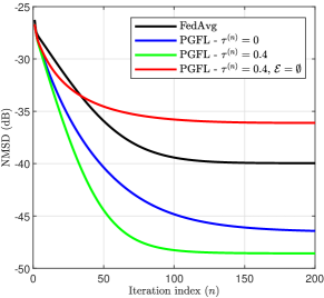
Figure 1: Learning curves of the PGFL algorithm with a fixed inter-cluster learning parameter and the FedAvg algorithm, without client scheduling or privacy.

Finally, we evaluate the aforementioned algorithms in a setting with client scheduling and privacy protection. All of the algorithms utilize zCDP with the noise perturbation presented in (11). Figure 3 shows the learning curves for the PGFL and FedAvg with client scheduling and privacy. We observe that the noise perturbation associated with differential privacy significantly reduces the convergence speed of all the simulated algorithms. However, we note that the NMSD after 300 iterations is nearly identical to the one in Fig. 2. This behavior is explained by the use of zCDP, in which the variance of the noise perturbation starts high and decreases linearly throughout the learning process.

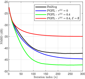
Figure 2: Learning curves of the PGFL algorithm with a fixed inter-cluster learning parameter and the FedAvg algorithm, considering client scheduling and without privacy.

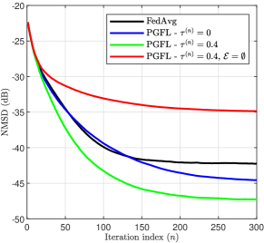
Figure 3: Learning curves of the PGFL algorithm with a fixed inter-cluster learning parameter and the FedAvg algorithm, considering client scheduling and privacy.

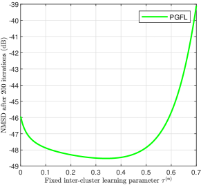
Figure 4: NMSD after $200$ iterations vs. fixed inter-cluster learning parameter $\tau^{(n)}$ values for the PGFL algorithm with client scheduling and privacy .

Further, we illustrate the importance of carefully choosing the value of the inter-cluster learning parameter. In Fig. 4, we simulated the proposed PGFL algorithm for various fixed $\tau^{(n)}$ values and displayed the NMSD after $200$ iterations. For instance, the NMSD for $\tau^{(n)}=0.4$ corresponds to the result obtained in Fig. 3. This figure confirms that inter-cluster learning has the potential to increase learning performance by alleviating data scarcity, as the PGFL algorithm achieves lower NMSD with $\tau^{(n)}\in(0.1,0.5)$ than with $\tau^{(n)}=0$. It also shows that the inter-cluster learning parameter must be carefully selected, as a value too large for the setting leads to performance degradation.

We then illustrate an alternative use of inter-cluster learning. For this experiment, the difference between the data distribution of the different clusters has been increased. Precisely, the datasets were simulated with the models obtained by ${\bf w}_{q}={\bf w}_{0}+\gamma{\bf w}_{0}$ with $\gamma\sim\mathcal{U}(-0.5,0.5)$. The learning curves are presented in Fig. 5. We observed that, because of the higher cluster dissimilarity, inter-cluster learning degrades steady-state NMSD; this is observed in the learning curves for PGFL with $\tau^{(n)}=0$ and $\tau^{(n)}=0.4$. However, by mitigating data scarcity within a cluster, inter-cluster learning improves the initial convergence rate. To benefit from an improved initial convergence rate and avoid steady-state performance degradation, it is possible to reduce the inter-cluster learning parameter progressively. Doing so, the PGFL algorithm with time-varying $\tau^{(n)}=0.4\times 0.98^{n}$ has the same initial convergence rate as the PGFL algorithm with fixed $\tau=0.4$ and attains near-identical steady-state NMSD as the PGFL algorithm with fixed $\tau=0$.

Finally, we study the impact of privacy protection on the steady-state NMSD of the PGFL algorithm. Fig. 6 shows the NMSD after $200$ iterations versus the initial value of the privacy parameter $\phi_{0}$. Note that, as seen in Theorem III, a lower value of $\phi_{0}$ ensures more privacy. We observe that for smaller values of $\phi_{0}$, the steady-state NMSE of the PGFL algorithm is higher. In fact, a lower total privacy loss bound leads to higher perturbation noise variance and diminishes the learning performance of the algorithm.

V-B Experiments for Classification on the MNIST Dataset

The following experiments were conducted on the MNIST handwritten digits dataset [53]. In those experiments, the learning tasks of the clients associated with different clusters share the same data but have different, related, objective functions. The structure of the server network, as well as the number of clients per server, are identical to the experiments for regression. In the following experiments, the clients of a given cluster use the ADMM for logistic regression to differentiate between two classes. The loss function for the logistic regression is given by

$$\log[\ell_{k}({\bf X}_{k},{\bf y}_{k};{\bf w}_{k})]=\frac{-1}{D_{k}} \sum_{i=1}^{D_{k}}\Bigl{(}y_{k,i}\log[y_{k,i}^{\prime}]$$

$$+(1-y_{k,i})\log[1-y_{k,i}^{\prime}]\Bigr{)},$$ (54)

with

$$y_{k,i}^{\prime}=\frac{1}{1+\exp(-{\bf w}_{k}^{\intercal}{\bf x}_{k,i})}.$$ (55)

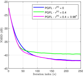
Figure 5: Learning curves of the PGFL algorithm with fixed and time-varying inter-cluster learning parameter $\tau^{(n)}$ in a setting with low cluster similarity, considering client scheduling and privacy.

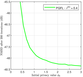
Figure 6: Privacy-accuracy trade-off of the PGFL algorithm with a fixed inter-cluster learning parameter, considering client scheduling.

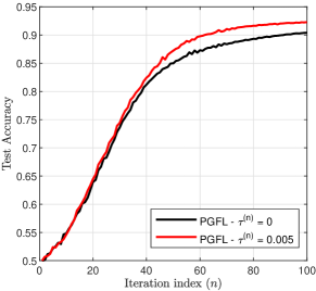
Figure 7: Test accuracy curve of the PGFL algorithm with a fixed inter-cluster learning parameter, considering client scheduling and privacy, with low cluster similarity.

We simulated the PGFL algorithm in the context of classification with client scheduling, privacy, a fixed inter-cluster learning parameter $\tau^{(n)}=\tau=0.4$, and without inter-cluster learning $\tau^{(n)}=0$. Figure 7 shows the test accuracy versus iteration index in a setting the clients of a given cluster must differentiate between two classes composed of a single digit. Each client receives between $D_{k}=2$ and $D_{k}=4$ data samples composed of two MNIST images. The clients of cluster $1$ have access to images of the digits $\{1\}$ and $\{8\}$. The clients of clusters $2$ and $3$ have access to images of the digits $\{1\}$ and $\{9\}$, and $\{7\}$ and $\{8\}$, respectively. Given that the clients of different clusters must differentiate between different digits, the similarity between the learning task is limited. Nevertheless, we observe that inter-cluster learning does improve the accuracy of the PGFL algorithm in this setting.

Further, we modified the setting so that the clusters exhibit more similarity. Figure 8 shows the test accuracy versus iteration index in a setting where the clients of a given cluster must differentiate between two classes composed of triplets of digits. Each client receives between $D_{k}=6$ and $D_{k}=12$ data samples, each composed of two triplets of MNIST images. The clients of cluster $1$ must differentiate between the classes $\{1,2,3\}$ and $\{6,7,8\}$, the clients of cluster $2$ between $\{1,2,3\}$ and $\{7,8,9\}$, and the clients of cluster $3$ between $\{1,2,3\}$ and $\{6,8,9\}$. We observe that, in this setting, inter-cluster learning significantly improves the accuracy of the PGFL algorithm.

Finally, we utilize the previous setting and evaluate the impact of the value of the inter-cluster learning parameter $\tau^{(n)}$ on the accuracy achieved by the PGFL algorithm in the context of classification. Figure 9 displays the accuracy achieved by the PGFL algorithm after $100$ iterations versus the value of the inter-cluster learning parameter in the context of the classification task of Fig. 8. We observe that, in this setting where the similarity among the learning tasks is high, medium and large fixed values for $\tau^{(n)}$ lead to significant accuracy improvement. However, very large values lead to performance degradation, similar to Fig. 4.

VI Conclusions

This paper proposed a framework for personalized graph federated learning in which distributed servers collaborate with each other and their respective clients to learn cluster-specific personalized models. The proposed framework leverages the similarities among clusters to improve learning speed and alleviate data scarcity. Further, this framework is implemented with the ADMM as a local learning process and with local zero-concentrated differential privacy to protect the participants’ data from eavesdroppers. Our mathematical analysis showed that this algorithm converges to the exact optimal solution for each cluster in linear time and that utilizing inter-cluster learning leads to an alternative output whose distance to the original solution is bounded by a value that can be adjusted with the inter-cluster learning parameter sequence. Finally, numerical simulations showed that the proposed method is capable of leveraging the graph federated architecture and the similarity between the clusters learning tasks to improve learning performance.

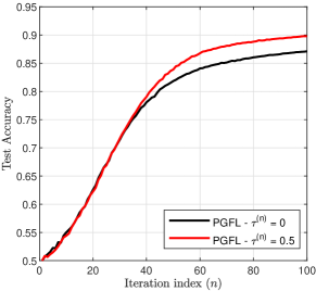
Figure 8: Test accuracy curve of the PGFL algorithm with a fixed inter-cluster learning parameter, considering client scheduling and privacy, with high cluster similarity.

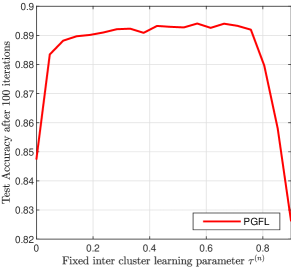
Figure 9: Test accuracy of the PGFL algorithm after $100$ iterations vs. fixed inter-cluster learning parameter $\tau^{(n)}$, considering client scheduling and privacy..

References

- [1] F. Gauthier, V. C. Gogineni, S. Werner, Y.-F. Huang, and A. Kuh, “Clustered graph federated personalized learning,” Asilomar Conf. Signals Syst. Comput., pp. 744–748, Oct. 2022.
- [2] J. Konečnỳ, H. B. McMahan, D. Ramage, and P. Richtárik, “Federated optimization: distributed machine learning for on-device intelligence,” arXiv preprint arXiv:1610.02527, Oct. 2016.
- [3] T. Li, A. K. Sahu, A. Talwalkar, and V. Smith, “Federated learning: challenges, methods, and future directions,” IEEE Signal Process. Mag., vol. 37, no. 3, pp. 50–60, May 2020.
- [4] S. Niknam, H. S. Dhillon, and J. H. Reed, “Federated learning for wireless communications: Motivation, opportunities, and challenges,” IEEE Commun. Mag., vol. 58, no. 6, pp. 46–51, Jun. 2020.
- [5] E. Rizk and A. H. Sayed, “A graph federated architecture with privacy preserving learning,” IEEE Int. Workshop Signal Process. Advances Wireless Commun., pp. 131–135, Sep. 2021.
- [6] L. Liu, J. Zhang, S. Song, and K. B. Letaief, “Client-edge-cloud hierarchical federated learning,” IEEE Int. Conf. Commun., pp. 1–6, Jun. 2020.
- [7] Y. Sarcheshmehpour, M. Leinonen, and A. Jung, “Federated learning from big data over networks,” IEEE Int. Conf. Acoust., Speech Signal Process., pp. 3055–3059, Jan. 2021.
- [8] V. C. Gogineni, S. Werner, Y.-F. Huang, and A. Kuh, “Decentralized graph federated multitask learning for streaming data,” Annu. Conf. Inf. Sciences Syst., pp. 101–106, Mar. 2022.
- [9] L. Li, Y. Fan, M. Tse, and K.-Y. Lin, “A review of applications in federated learning,” Computers & Ind. Eng., vol. 149, p. 106854, 2020.
- [10] B. Yang, X. Cao, K. Xiong, C. Yuen, Y. L. Guan, S. Leng, L. Qian, and Z. Han, “Edge intelligence for autonomous driving in 6G wireless system: Design challenges and solutions,” IEEE Wireless Commun., vol. 28, no. 2, pp. 40–47, Apr. 2021.
- [11] S. Boll and J. Meyer, “Health-X dataLOFT: a sovereign federated cloud for personalized health care services,” IEEE MultiMedia, vol. 29, no. 1, pp. 136–140, May 2022.
- [12] A. Z. Tan, H. Yu, L. Cui, and Q. Yang, “Towards personalized federated learning,” IEEE Trans. Neural Networks Learning Syst., Mar. 2022.
- [13] C. T Dinh, N. Tran, and J. Nguyen, “Personalized federated learning with moreau envelopes,” Advances Neural Inf. Process. Syst., vol. 33, pp. 21 394–21 405, 2020.
- [14] C. J. Felix, J. Ye, and A. Kuh, “Personalized learning using kernel methods and random fourier features,” Int. Joint Conf. Neural Netw., pp. 1–5, Jul. 2022.
- [15] V. C. Gogineni, S. Werner, F. Gauthier, Y.-F. Huang, and A. Kuh, “Personalized online federated learning for IoT/CPS: challenges and future directions,” IEEE Internet Things Mag., 2022.
- [16] A. Fallah, A. Mokhtari, and A. Ozdaglar, “Personalized federated learning: a meta-learning approach,” arXiv preprint arXiv:2002.07948, Feb. 2020.
- [17] Y. Deng, M. M. Kamani, and M. Mahdavi, “Adaptive personalized federated learning,” arXiv preprint arXiv:2003.13461, Mar. 2020.
- [18] J. Chen, C. Richard, and A. H. Sayed, “Multitask diffusion adaptation over networks,” IEEE Trans. Signal Process., vol. 62, no. 16, pp. 4129–4144, Jun. 2014.
- [19] V. C. Gogineni and M. Chakraborty, “Improving the performance of multitask diffusion APA via controlled inter-cluster cooperation,” IEEE Trans. Circuits Syst. I: Reg. Papers, vol. 67, no. 3, pp. 903–912, Dec. 2019.
- [20] A. Ghosh, J. Chung, D. Yin, and K. Ramchandran, “An efficient framework for clustered federated learning,” Advances Neural Info. Process. Syst., vol. 33, pp. 19 586–19 597, 2020.
- [21] D. Caldarola, M. Mancini, F. Galasso, M. Ciccone, E. Rodolà, and B. Caputo, “Cluster-driven graph federated learning over multiple domains,” Proc.IEEE Conf. Comput. Vision Pattern Recognit., pp. 2749–2758, 2021.
- [22] F. Sattler, K.-R. Müller, and W. Samek, “Clustered federated learning: Model-agnostic distributed multitask optimization under privacy constraints,” IEEE Trans. Neural Netw. Learn. Syst., vol. 32, no. 8, pp. 3710–3722, Aug. 2020.
- [23] V. Smith, C.-K. Chiang, M. Sanjabi, and A. S. Talwalkar, “Federated multi-task learning,” Advances Neural Inf. Process. Syst., vol. 30, . 2017.
- [24] R. Li, F. Ma, W. Jiang, and J. Gao, “Online federated multitask learning,” IEEE Int. Conf. Big Data, pp. 215–220, Dec. 2019.
- [25] A. Taïk and S. Cherkaoui, “Electrical load forecasting using edge computing and federated learning,” IEEE Int. Conf. Commun., Jun. 2020.
- [26] F.-Z. Lian, J.-D. Huang, J.-X. Liu, G. Chen, J.-H. Zhao, and W.-X. Kang, “FedFV: A personalized federated learning framework for finger vein authentication,” Machine Intel. Research, pp. 1–14, Jan. 2023.
- [27] S. Wang, S. Hosseinalipour, M. Gorlatova, C. G. Brinton, and M. Chiang, “UAV-assisted online machine learning over multi-tiered networks: A hierarchical nested personalized federated learning approach,” IEEE Trans. Netw. Service Manage., Oct. 2022.
- [28] A. M. G. Salem, A. Bhattacharyya, M. Backes, M. Fritz, and Y. Zhang, “Updates-leak: Data set inference and reconstruction attacks in online learning,” 29th USENIX Secur. Symp., pp. 1291–1308, Aug. 2020.
- [29] K. Wei, J. Li, M. Ding, C. Ma, H. H. Yang, F. Farokhi, S. Jin, T. Q. Quek, and H. V. Poor, “Federated learning with differential privacy: algorithms and performance analysis,” IEEE Trans. Inf. Forensics Secur., vol. 15, pp. 3454–3469, Apr. 2020.
- [30] C. Dwork, F. McSherry, K. Nissim, and A. Smith, “Calibrating noise to sensitivity in private data analysis,” in Proc. Conf. Theory Cryptography, 2006, pp. 265–284.
- [31] J. Cortés, G. E. Dullerud, S. Han, J. Le Ny, S. Mitra, and G. J. Pappas, “Differential privacy in control and network systems,” in IEEE 55th Conf. Decision Control, Dec. 2016, pp. 4252–4272.
- [32] C. Dwork and A. Roth, “The Algorithmic Foundations of Differential Privacy,” Found. Trends Theor. Comput. Sci., vol. 9, pp. 211–407, Aug. 2014.
- [33] K. Wei, J. Li, M. Ding, C. Ma, H. H. Yang, F. Farokhi, S. Jin, Q. S. Tony Quek, and H. Vincent Poor, “Federated learning with differential privacy: Algorithms and performance analysis,” IEEE Trans. Inf. Forensics Secur., vol. 15, pp. 3454–3469, Apr. 2020.
- [34] P. Kairouz, S. Oh, and P. Viswanath, “The composition theorem for differential privacy,” Int. Conf. Machine Learn., pp. 1376–1385, Jun. 2015.
- [35] C. Dwork and G. N. Rothblum, “Concentrated differential privacy,” arXiv preprint arXiv:1603.01887, 2016.
- [36] M. Bun and T. Steinke, “Concentrated Differential Privacy: Simplifications, Extensions, and Lower Bounds,” in Theory of Cryptography Conf. Springer, 2016, pp. 635–658.
- [37] X. Lyu, “Composition theorems for interactive differential privacy,” arXiv preprint arXiv:2207.09397, Jul. 2022.
- [38] J. Ding, Y. Gong, M. Pan, and Z. Han, “Optimal differentially private ADMM for distributed machine learning,” Available at http://arxiv.org/abs/1901.02094, Feb. 2019.
- [39] R. Hu, Y. Guo, and Y. Gong, “Concentrated differentially private federated learning with performance analysis,” IEEE Open J. Comput. Soc., pp. 276–289, Jul. 2021.
- [40] F. Gauthier, C. Gratton, N. K. Venkategowda, and S. Werner, “Privacy-preserving distributed learning with nonsmooth objective functions,” IEEE 54th Asilomar Conf. Signals, Syst., Computers, pp. 42–46, Nov. 2020.
- [41] S. Zhou and G. Y. Li, “Federated learning via inexact ADMM,” IEEE Trans. Pattern Anal. Machine Intell., Feb. 2023.
- [42] Y. Chen, R. S. Blum, and B. M. Sadler, “Communication efficient federated learning via ordered ADMM in a fully decentralized setting,” Conf. Inf. Sciences Syst., pp. 96–100, Mar. 2022.
- [43] S. Yue, J. Ren, J. Xin, S. Lin, and J. Zhang, “Inexact-ADMM based federated meta-learning for fast and continual edge learning,” in Proc. Int. Symp. Theory Algorithmic Found. Protocol Des. Mobile Netw. Mobile Comput. Assoc. Comput. Mach., Jul. 2021, p. 91–100.
- [44] W. Shi, Q. Ling, K. Yuan, G. Wu, and W. Yin, “On the linear convergence of the ADMM in decentralized consensus optimization,” IEEE Trans. Signal Process., vol. 62, no. 7, pp. 1750–1761, 2014.
- [45] J. Ding, X. Zhang, M. Chen, K. Xue, C. Zhang, and M. Pan, “Differentially Private Robust ADMM for Distributed Machine Learning,” in 2019 IEEE Int. Conf. Big Data, Dec. 2019, pp. 1302–1311.
- [46] S. Ben-David and R. Schuller, “Exploiting task relatedness for multiple task learning,” Conf. Learn. Theory Kernel Workshop, pp. 567–580, Aug. 2003.
- [47] G. B. Giannakis, Q. Ling, G. Mateos, and I. D. Schizas, “Splitting Methods in Communication, Imaging, Science, and Engineering,” in Scientific Computation. Springer Int. Publishing, Jan. 2017, pp. 461–497.
- [48] J. Chen, C. Richard, and A. H. Sayed, “Multitask diffusion adaptation over networks,” IEEE Trans. Signal Process., vol. 62, no. 16, pp. 4129–4144, Jun. 2014.
- [49] V. C. Gogineni and M. Chakraborty, “Diffusion affine projection algorithm for multitask networks,” Asia-Pacific Signal Inf. Process. Assoc. Annu. Summit Conf., pp. 201–206, Nov. 2018.
- [50] C. Dwork, N. Kohli, and D. Mulligan, “Differential privacy in practice: expose your epsilons!” J. Privacy Confidentiality, vol. 9, no. 2, Oct. 2019.
- [51] Q. Li, B. Kailkhura, R. Goldhahn, P. Ray, and P. K. Varshney, “Robust decentralized learning using ADMM with unreliable agents,” arXiv preprint arXiv:1710.05241, Oct. 2017.
- [52] B. McMahan, E. Moore, D. Ramage, S. Hampson, and B. A. y Arcas, “Communication-efficient learning of deep networks from decentralized data,” Artificial Intel. Statis., pp. 1273–1282, Apr. 2017.
- [53] L. Deng, “The MNIST database of handwritten digit images for machine learning research,” IEEE Signal Process. Mag., vol. 29, no. 6, pp. 141–142, 2012.