On the characterization of formal automorphisms of integro-differential operators

Abstract

Necessary and sufficient conditions on a family of integro-differential operators to determine a formal automorphism are established. Equivalently, the problem can be read in terms of existence and uniqueness of formal solutions of Cauchy problems in different settings.

The main results provide a characterization not only in the framework of general formal power series, but also on subspaces appearing in applications such as Gevrey settings and moment differential operators.

Key words: formal automorphism, integro-differential operator, Newton polygon Gevrey series, moment differential. 2020 MSC: 35C10, 35G10

1 Introduction

In the present work, we study necessary and sufficient conditions for integro-differential operators of the form $P(\partial_{t},\partial_{z})\partial_{t}^{-m}$ to define a linear automorphism when acting on different spaces of formal power series. Here, $P$ stands for a polynomial in two variables, and $m$ is a positive integer.

This problem naturally arises when studying the existence and uniqueness of formal solutions to differential Cauchy problems. In this sense, assume that $P(\partial_{t},\partial_{z})$ is a general differential operator in two complex variables $(t,z)\in\mathbb{C}^{2}$ with variable coefficients that belong to the space of formal power series in the variables $(t,z)$, say $\mathbb{C}[[t,z]]$, or in particular to the space of formal power series in the variable $t$, with coefficients being holomorphic functions on some common neighborhood of the origin, say $\mathcal{O}[[t]]$. Let us write it in the form

(1) $$P(\partial_{t},\partial_{z})=\sum_{(j,r)\in\Lambda}a_{jr}(t,z)\partial_{t}^{j}\partial_{z}^{r},$$

where $\Lambda\subset\mathbb{N}_{0}\times\mathbb{N}_{0}:=\{0,1,\ldots\}\times\{0,1,\ldots\}$ is a finite set of indices and $a_{jr}(t,z)\in\mathcal{O}[[t]]$ (resp. $a_{jr}(t,z)\in\mathbb{C}[[t,z]]$) for every $(j,r)\in\Lambda$.

For fixed $m\in\mathbb{N}_{0}$ one can consider the Cauchy problem

$$\left\{\begin{array}[]{l}P(\partial_{t},\partial_{z})u(t,z)=f(t,z)\\ \partial_{t}^{j}u(0,z)=\varphi_{j}(z)\quad\textrm{for}\quad j=0,\dots,m-1\end{array}\right..$$

For such Cauchy problem, natural questions arise on the existence and unicity of formal solutions. More precisely, we will focus on finding necessary and sufficient conditions on the operator $P(\partial_{t},\partial_{z})$ given by (1), under which statement (A) holds or both statements (A) and (B) hold.

1. For every $f(t,z)\in\mathbb{C}[[t,z]]$ and every $\varphi_{j}(z)\in\mathbb{C}[[z]]$ ($j=0,\dots,m-1$) there exists exactly one solution $u(t,z)\in\mathbb{C}[[t,z]]$.

2. Fix $s\geq 0$. For every $f(t,z)\in G_{s}[[t]]$ and every $\varphi_{j}(z)\in\mathbb{C}[[z]]_{s}$ ($j=0,\dots,m-1$) there exists exactly one solution $u(t,z)\in G_{s}[[t]]$.

Here, $G_{s}$ stands for the Banach space of formal power series such that its Borel transform of order $s$ defines a series with positive radius of convergence (see Definition 1), and $G_{s}[[t]]$ denotes the space of formal power series in $t$ with coefficients in the Banach space $G_{s}$. The previous Banach space is known as the space of Gevrey series, which has proved to have an essential importance in the development of the classical theory of summability of formal solutions to functional equations. We refer to [1, 12] for a further and broad reading on the topic.

Observe that the statement (A) can be reformulated by saying that the integro-differential operator

(2) $$P(\partial_{t},\partial_{z})\partial_{t}^{-m}\colon\mathbb{C}[[t,z]]\to\mathbb{C}[[t,z]]$$

is a linear automorphism.

Analogously, given $s\geq 0$, the statement (B) can be reformulated by saying that the integro-differential operator

(3) $$P(\partial_{t},\partial_{z})\partial_{t}^{-m}\colon G_{s}[[t]]\to G_{s}[[t]]$$

is a linear automorphism.

For this reason, the main results in the present work are focused on giving the necessary and sufficient conditions on $P(\partial_{t},\partial_{z})$ under which operator (2) is an automorphism, and both operators (2) and (3) are automorphisms. The main results in the present work give answer to the previous questions in Theorem 3 and Theorem 4, respectively.

Moreover, we discuss the extensions of the above characterization to the moment integro-differential operators

$$P(\partial_{\mathfrak{m}_{1},t},\partial_{\mathfrak{m}_{2},z})\partial_{\mathfrak{m}_{1},t}^{-m},$$

where $\partial_{\mathfrak{m}_{1},t}$ and $\partial_{\mathfrak{m}_{2},z}$ are moment differential operators defined for given sequences of positive numbers $\mathfrak{m}_{1}$ and $\mathfrak{m}_{2}$ (see Section 3.1 for the definition of moment differential operators).

The study of existence and uniqueness of formal solutions to a given partial differential equation has a significant role in the knowledge of analytic solutions to the problem. Roughly speaking, the theory of summability departs from an existing formal power series solving the problem and constructs the analytic solution by means of a summability procedure, known as Borel-Laplace procedure in its most classical version.

Therefore, the existence of a formal solution to the problem is major.

On the other hand, the relationship between the analytic and the formal solutions usually arises in the form of an asymptotic expansion. The formal solution is a formal power series with possibly null radius of convergence, and its truncation approximates the analytic solution when working on adequate domains on the complex plane, which are typically bounded sectors with vertex at the origin (or the point where the formal asymptotic expansion has been chosen to be performed).

Uniqueness of the formal solution to the problem is also important as it is the input in the procedure mentioned above.

The strategy followed is to reduce the problem to linear automorphisms of formal differential equations of one variable of the form

$$P(\partial_{z})=\sum_{j\in\Gamma}a_{j}(z)\partial_{z}^{j},$$

for some polynomial $P$ with coefficients holomorphic near the origin. The result obtained (Theorem 1) describes a characterization of $P$ to be a linear automorphism on $\mathbb{C}[[z]]$ in term of geometric aspects related to the Newton polygon associated with $P$, together with a non-resonance condition on the characteristic polynomial associated with $P$. Another characterization is also obtained when studying linear automorphisms on Gevrey formal power series in one variable (Theorem 2) in terms of additional geometric properties satisfied by the Newton polygon of $P$. The convergent case follows as a direct corollary. The results are then applied in the two variable setting in Section 4 to achieve the main results (Theorem 3 and Theorem 4). We conclude the work by linking our results to previous known results in a different context.

In the last few years years, new advances in this theory were achieved in recent studies on the formal solutions to partial differential equations in the complex domain and their summability, such as [13, 20, 25], among many others.

Additionally, knowing upper estimates for the coefficients of the formal solution of a differential problem is useful at the time of determining a Gevrey order of the solution in order to apply an appropriate Borel transform to the formal power series. Therefore, the existence of an automorphism in Gevrey settings provides the knowledge of Gevrey upper bounds associated with the solution, when departing from a known upper bound of the Gevrey order of the forcing term $f$. Such results are known as Maillet-type theorems, and also remain an active field of research of complex partial differential equations. See [11, 22] among others, and the references therein.

We are also exploring the generalization of the main results in the present work in the framework of partial moment differential equations, as mentioned above, due to the relevance that operators of this kind have been acquiring in the last decade. Recent results on the summability of formal solutions to such equations are [9, 10, 16], and also on results of Maillet type in [8, 23].

The paper is structured as follows. In Section 2 we state preliminary definitions and results. It is followed by Section 3, devoted to the study of the problem in the one variable setting, including several examples of the different situations appearing. A single subsection (Section 3.1) is set aside to describe the more general case of moment differential operators in one variable, and another (Section 3.2) focuses on automorphisms under Gevrey settings. In the main section of the present work, Section 4, we state the main results achieved, Theorem 3 and Theorem 4.

Notation:

$\mathbb{N}$ stands for the set of positive integers, and $\mathbb{N}_{0}=\mathbb{N}\cup\{0\}$.

Let $r>0$. $D_{r}$ stands for the open disc centered at the origin and radius $r$, it is to say, $D_{r}=\{z\in\mathbb{C}:|z|<r\}$.

Given an open set $U\subseteq\mathbb{C}$, we denote by $\mathcal{O}(U)$ the set of holomorphic functions defined in $U$. Given a set $A\subseteq\mathbb{C}$, $C(A)$ stands for the set of continuous functions in $A$ to complex values. The set of formal power series with coefficients in a nonempty set $A$ (in the variable $t$) is denoted by $A[[t]]$. The set of formal power series in $t$ with coefficients being holomorphic functions on some common neighborhood of the origin will be denoted by $\mathcal{O}[[t]]$. $\mathbb{C}[[t]]$ stands for the vector space of formal power series with coefficients in $\mathbb{C}$, whereas $\mathbb{C}\{t\}\subseteq\mathbb{C}[[t]]$ represents the subspace of convergent formal power series. We also write $\mathbb{C}[z]$ for the set of polynomials with complex coefficients (in the variable $z$).

2 Preliminary definitions and results

In this section, we recall the main definitions and known results to be used in the present work. We mainly work with the space of formal power series with complex coefficients of some Gevrey order $s\geq 0$, denoted by $\mathbb{C}[[z]]_{s}$, which consists of all formal power series $\sum_{n=0}^{\infty}\varphi_{n}z^{n}\in\mathbb{C}[[z]]$ such that there exist $C,A>0$ with

$$|\varphi_{n}|\leq CA^{n}\Gamma(1+sn),\quad n\geq 0.$$

Here, $\Gamma(\cdot)$ stands for Gamma function.

The next definition can be found in [15], Definition 7.

Definition 1

Fix $r>0$ and $s\geq 0$. By $G_{s}(r)$ we denote the Banach space of Gevrey series

$$G_{s}(r):=\left\{\varphi(z)=\sum_{n=0}^{\infty}\varphi_{n}z^{n}\in\mathbb{C}[[z]]_{s}\colon\mathcal{B}_{\Gamma_{s},z}\varphi(z):=\sum_{n=0}^{\infty}\frac{\varphi_{n}}{\Gamma(1+sn)}z^{n}\in\mathcal{O}(D_{r})\cap C(\overline{D_{r}})\right\}$$

equipped with the norm

$$\|\varphi\|_{G_{s}(r)}:=\max_{|z|\leq r}|\mathcal{B}_{\Gamma_{s},z}\varphi(z)|.$$

Observe that, given $s\geq 0$, for every $\varphi\in\mathbb{C}[[z]]_{s}$, there exists $r>0$ such that $\varphi\in G_{s}(r)$.

We also set $G_{s}:=\varinjlim\limits_{r>0}G_{s}(r)$ as the inductive limit of the previous Banach spaces with respect to $r$. We observe that the space of formal power series in $G_{0}[[t]]$ coincides with the space of analytic functions defined on some neighborhood of the origin, $\mathcal{O}[[t]]$, by identification of each element with its Taylor expansion.

Let $P\in\mathbb{C}[t]$ and consider the formal differential operator $P(\partial_{z})$ acting on $\mathbb{C}[[z]]$. Here, $\partial_{z}$ stands for the formal differentiation operator.

Definition 2

The index $\chi$ of the operator $P(\partial_{z})\colon\mathbb{C}[[z]]\to\mathbb{C}[[z]]$ is defined as

$$\chi(P(\partial_{z}),\mathbb{C}[[z]]):=\dim\ker(P(\partial_{z}),\mathbb{C}[[z]])-\dim\mathrm{coker}(P(\partial_{z}),\mathbb{C}[[z]]),$$

where

$$\ker(P(\partial_{z}),\mathbb{C}[[z]]):=\{u\in\mathbb{C}[[z]]:\ P(\partial_{z})u(z)=0\},$$

$$\mathrm{im}(P(\partial_{z}),\mathbb{C}[[z]])=\{f\in\mathbb{C}[[z]]:\ P(\partial_{z})u(z)=f(z)\ \textrm{for some}\ u\in\mathbb{C}[[z]]\}$$

and

$$\mathrm{coker}(P(\partial_{z}),\mathbb{C}[[z]])=\mathbb{C}[[z]]/\mathrm{im}(P(\partial_{z}),\mathbb{C}[[z]]).$$

Analogously, the index $\chi$ of the operator $P(\partial_{z})$ can be defined when restricting the previous operator to $\mathbb{C}[[z]]_{s}$ for any fixed $s\geq 0$. By maintaining the same notation for such restriction, we observe that $P(\partial_{z})\colon\mathbb{C}[[z]]_{s}\to\mathbb{C}[[z]]_{s}$ for any fixed $s\geq 0$ (see for example Proposition 1.2.4, [12], together with Stirling’s formula).

3 Linear automorphisms of formal differential operators of one variable

In this section, we state equivalent conditions for a formal operator $P(\partial_{z}):\mathbb{C}[[z]]\to\mathbb{C}[[z]]$ (resp. $P(\partial_{z}):\mathbb{C}[[z]]_{s}\to\mathbb{C}[[z]]_{s}$) to be an automorphism, for some given polynomial $P$ with coefficients given by analytic functions near the origin (resp. some given polynomial $P$ with coefficients given by analytic functions near the origin, and some fixed $s\geq 0$). The main results of the present work, dealing with formal differential operators in two variables, lean on those developed in this section.

Let $\Lambda\subset\mathbb{N}_{0}$ be a finite set of indices and let

(4) $$P(\partial_{z})=\sum_{j\in\Lambda}a_{j}(z)\partial_{z}^{j}$$

be a differential operator of order $p\in\mathbb{N}$ with holomorphic coefficients on some neighborhood of the origin, say $D$. The order of the zero of $a_{j}(z)$ at $z=0$ is denoted by $\alpha_{j}:=\mathrm{ord}_{z}(a_{j})$. Therefore, we may write

(5) $$a_{j}(z)=\sum_{k\geq\alpha_{j}}a_{j,k}z^{k}\in\mathcal{O}(D),$$

for every $j\in\Lambda$.

Following [17], we define the Newton polygon of the operator $P(\partial_{z})$ as the convex hull of the union of sets $\mathbin{\vrule height=0.55974pt,depth=0.0pt,width=5.59721pt\vrule height=6.88889pt,depth=0.0pt,width=0.55974pt}\,(j,\alpha_{j}-j)$ for $j\in\Lambda$,

(6) $$N(P):=\mathrm{conv}\left\{\bigcup_{j\in\Lambda}\mathbin{\vrule height=0.55974pt,depth=0.0pt,width=5.59721pt\vrule height=6.88889pt,depth=0.0pt,width=0.55974pt}\,(j,\alpha_{j}-j)\right\},$$

where $\mathbin{\vrule height=0.55974pt,depth=0.0pt,width=5.59721pt\vrule height=6.88889pt,depth=0.0pt,width=0.55974pt}\,(a,b):=\{(x,y)\in\mathbb{R}^{2}\colon x\leq a,\ y\geq b\}$ denotes the second quadrant of $\mathbb{R}^{2}$ translated by the vector $(a,b)$.

The number

$$m:=\min_{j\in\Lambda}(\alpha_{j}-j)\in\mathbb{Z}$$

denotes the lower ordinate of the Newton polygon $N(P)$ of the operator $P(\partial_{z})$.

Remark: Observe that, if $L_{m}:=\{(x,y)\in\mathbb{R}^{2}\colon y=m\}$ then

$$L_{m}\cap N(P)=L_{m}\cap\partial N(P)\subseteq\{(x,y)\in\mathbb{R}^{2}\colon x\leq p,\ y=m\}.$$

Definition 3

Given $P$ as before, the principal part $P_{-m}(\partial_{z})$ of the operator $P(\partial_{z})$ is defined as

(7) $$P_{-m}(\partial_{z}):=\sum_{j\in\Lambda_{m}}a_{j,j+m}z^{j+m}\partial_{z}^{j},\quad\textrm{where}\quad\Lambda_{m}:=\{j\in\Lambda:\ \alpha_{j}-j=m\}.$$

We also define the characteristic polynomial of the operator $P(\partial_{z})$ as

(8) $$W_{m}(\lambda):=\sum_{j\in\Lambda_{m}}a_{j,j+m}\cdot\lambda\cdot\ldots\cdot(\lambda-j+1).$$

Theorem 1

The operator $P(\partial_{z})$ is a linear automorphism on $\mathbb{C}[[z]]$ if and only if the following conditions hold:

1. The lower ordinate $m$ of the Newton polygon $N(P)$ is equal to zero.

2. (non-resonance condition) The characteristic polynomial $W_{0}(n)$ of the operator $P(\partial_{z})$ is different from zero for every $n\in\mathbb{N}_{0}$.

Proof We consider the equation

(9) $$P(\partial_{z})u(z)=f(z),\quad\textrm{where}\quad u(z)=\sum_{n=0}^{\infty}u_{n}z^{n}\in\mathbb{C}[[z]]\quad\textrm{and}\quad f(z)=\sum_{n=0}^{\infty}f_{n}z^{n}\in\mathbb{C}[[z]].$$

It is worth providing a previous reasoning to the proof that helps in understanding the procedure of determining the existence and/or uniqueness of a formal power series $u(z)\in\mathbb{C}[[z]]$ to satisfy an equation of the form (9), for any given $f(z)\in\mathbb{C}[[z]]$.

First, observe that the operator $P(\partial_{z})$ is a linear automorphism on $\mathbb{C}[[z]]$ if and only if for every $f\in\mathbb{C}[[z]]$ there exists exactly one $u\in\mathbb{C}[[z]]$ satisfying (9), if and only if $\dim\ker(P(\partial_{z}),\mathbb{C}[[z]])=0$ and $\dim\mathrm{coker}(P(\partial_{z}),\mathbb{C}[[z]])=0$.

For $u(z)=\sum_{n=0}^{\infty}u_{n}z^{n}\in\mathbb{C}[[z]]$ we get

(10) $$P_{-m}(\partial_{z})u(z)=\sum_{j\in\Lambda_{m}}a_{j,j+m}z^{j+m}\partial_{z}^{j}\left(\sum_{n=0}^{\infty}u_{n}z^{n}\right)\\ =\sum_{n=0}^{\infty}\left(\sum_{j\in\Lambda_{m}}a_{j,j+m}n\cdot\ldots\cdot(n-j+1)\right)u_{n}z^{n+m}=\sum_{n=0}^{\infty}W_{m}(n)u_{n}z^{n+m}.$$

On the other hand, we consider the rest of the operator $P(\partial_{z})$, denoted by $\tilde{P}(\partial_{z})$ and defined by

$$\tilde{P}(\partial_{z}):=P(\partial_{z})-P_{-m}(\partial_{z}).$$

We may write this operator as

$$\tilde{P}(\partial_{z})=\sum_{j\in\tilde{\Lambda}}\tilde{a}_{j}(z)\partial_{z}^{j}$$

for some finite set of indices $\tilde{\Lambda}\subset\mathbb{N}_{0}$ and some $\tilde{a}_{j}(z)\in\mathcal{O}(D)$ for $j\in\tilde{\Lambda}$.

It is straightforward to check that $N(\tilde{P})\subset N(P)$ and $N(\tilde{P})\cap L_{m}=\emptyset$. More precisely, if we put $\tilde{\alpha}_{j}:=\mathrm{ord}_{z}(\tilde{a}_{j})$ we conclude that

$$\tilde{\alpha}_{j}-j\geq m+1\quad\textrm{for every}\quad j\in\tilde{\Lambda}.$$

Hence, we may write $\tilde{a}_{j}(z)$ as

$$\tilde{a}_{j}(z)=\sum_{k=m+1}^{\infty}\tilde{a}_{j,j+k}z^{j+k}.$$

This entails that for every $u(z)=\sum_{n=0}^{\infty}u_{n}z^{n}\in\mathbb{C}[[z]]$ we get

(11) $$\tilde{P}(\partial_{z})u(z)=\sum_{j\in\tilde{\Lambda}}\sum_{k=m+1}^{\infty}\tilde{a}_{j,j+k}z^{j+k}\partial_{z}^{j}\left(\sum_{n=0}^{\infty}u_{n}z^{n}\right)\\ =\sum_{n=0}^{\infty}\sum_{k=m+1}^{\infty}\left(\sum_{j\in\tilde{\Lambda}}\tilde{a}_{j,j+k}n\cdot\ldots\cdot(n-j+1)\right)u_{n}z^{n+k}=\sum_{n=0}^{\infty}\sum_{k=m+1}^{\infty}\tilde{W}_{m,k}(n)u_{n}z^{n+k},$$

where $\tilde{W}_{m,k}(n):=\sum_{j\in\tilde{\Lambda}}\tilde{a}_{j,j+k}\cdot n\cdot\ldots\cdot(n-j+1)$.

If we plug $u(z)=\sum_{n=0}^{\infty}u_{n}z^{n}$ into the equation

$$P(\partial_{z})u(z)=P_{-m}(\partial_{z})u(z)+\tilde{P}(\partial_{z})u(z)=f(z)=\sum_{n=0}^{\infty}f_{n}z^{n}\in\mathbb{C}[[z]],$$

and we compare the coefficients at $z^{n+m}$ (for $n\geq 0$ and $n+m\geq 0$) , by (10) and (11), we conclude that

(12) $$W_{m}(n)u_{n}=f_{n+m}-\sum_{k=m+1}^{m+n}\tilde{W}_{m,k}(n-k+m)u_{n-k+m}=f_{n+m}-\sum_{j=1}^{n}\tilde{W}_{m,m+j}(n-j)u_{n-j}\\ =:A_{m,n}(u_{0},\dots,u_{n-1},f_{n+m}),$$

where $A_{m,n}\in L(\mathbb{R}^{n+1},\mathbb{R})$ is a linear form on $\mathbb{R}^{n+1}$.

Hence, we conclude that the coefficient $u_{n}$ is uniquely determined by (12) if and only if

(13) $$W_{m}(n)\neq 0\quad\textrm{for every}\quad n\geq 0\quad\textrm{and}\quad n\geq-m.$$

This means that (13) is a necessary condition for $P(\partial_{z})$ to be a linear automorphism on $\mathbb{C}[[z]]$. In this case we get

(14) $$u_{n}=\frac{1}{W_{m}(n)}A_{m,n}(u_{0},\dots,u_{n-1},f_{n+m})\quad\textrm{for}\quad n\geq 0\quad\textrm{and}\quad n\geq-m.$$

In order to achieve surjectivity of $P(\partial_{z})$, i.e., whether for any given sequence $(f_{n})_{n\geq 0}\in\mathbb{C}^{N_{0}}$ there exists a uniquely determined sequence $(u_{n})_{n\geq 0}\in\mathbb{C}^{\mathbb{N}_{0}}$ satisfying (14), we consider two situations.

First, we assume that $m\leq 0$. Then by (14) the coefficients $u_{n}$ are uniquely determined only for $n>-m-1$. In particular this means that for any initial data $u_{0},\ldots,u_{-m-1}$ we can find uniquely determined $u(z)=\sum_{n=0}^{\infty}u_{n}z^{n}$ satisfying $P(\partial_{z})u=0$. Hence $\dim\ker(P(\partial_{z}),\mathbb{C}[[z]])=-m$. On the other hand, for every sequence $(f_{n})_{n\geq 0}$ one can find a sequence $(u_{n})_{n\geq 0}$ satisfying (14). This means that $\mathrm{im}(P(\partial_{z}),\mathbb{C}[[z]])=\mathbb{C}[[z]]$, so $\dim\mathrm{coker}(P(\partial_{z}),\mathbb{C}[[z]])=0$.

Next, we assume that $m\geq 0$. Then the sequence $(u_{n})_{n\geq 0}$ is uniquely determined by (14) and as a consequence $\dim\ker(P(\partial_{z}),\mathbb{C}[[z]])=0$. On the other hand, by (10) and (11) we see that $\mathrm{im}(P(\partial_{z}),\mathbb{C}[[z]])=z^{m}\mathbb{C}[[z]]$, so $\dim\mathrm{coker}(P(\partial_{z}),\mathbb{C}[[z]])=m$.

Observe also that in both cases (see also [12, Corollary 4.25]) we get

(15) $$\chi(P(\partial_{z}),\mathbb{C}[[z]])=-m.$$

The proof is straightforward after the previous reasoning.

($\Rightarrow$) Assume that $P(\partial_{z})$ is a linear automorphism on $\mathbb{C}[[z]]$. Since $P(\partial_{z})$ satisfies (15), one has $m=0$. Moreover, since (13) holds, we conclude that $W_{0}(n)\neq 0$ for every $n\in\mathbb{N}_{0}$.

($\Leftarrow$) If $m=0$ and $W_{0}(n)\neq 0$ for every $n\in\mathbb{N}_{0}$ then it follows from the above considerations that $u_{n}$ is uniquely determined by (14) for every $n\geq 0$, $\dim\ker(P(\partial_{z}),\mathbb{C}[[z]])=0$ and $\dim\mathrm{coker}(P(\partial_{z}),\mathbb{C}[[z]])=0$. Hence $P(\partial_{z})$ is a linear automorphism on $\mathbb{C}[[z]]$. $\Box$

The reasoning followed in the proof of the previous result can be applied to the following concrete examples.

Example 1

Let $a,b>0$. We consider the operator $P(\partial_{z}):\mathbb{C}[[z]]\to\mathbb{C}[[z]]$ given by

$$P(\partial_{z})=a+bz\partial_{z}+z^{3}\partial_{z}^{2}.$$

Its Newton polygon is represented in Figure 1 (left). We observe that $m=0$ so condition (a) in Theorem 1 applies, $\Lambda=\{0,1,2\}$ and $\Lambda_{m}=\{0,1\}$. It holds that $P_{-m}(\partial_{z})=a+bz\partial_{z}$ and $W_{m}(\lambda)=a+b\lambda$. Notice that $W_{m}(n)\neq 0$ for any $n\in\mathbb{N}_{0}$ so condition (b) in Theorem 1 is satisfied. Theorem 1 guarantees that $P(\partial_{z})$ is an automorphism of $\mathbb{C}[[z]]$. Given $f(z)=\sum_{n=0}^{\infty}f_{n}z^{n}\in\mathbb{C}[[z]]$ the only formal power series $u(z)=\sum_{n=0}^{\infty}u_{n}z^{n}$ such that $P(\partial_{z})u=f$ is determined as follows: $u_{0}=f_{0}/a$, $u_{1}=f_{1}/(a+b)$, $u_{2}=f_{2}/(a+2b)$, and $u_{n}=(f_{n}-(n-1)(n-2)u_{n-1})/(a+bn)$ for $n\geq 3$.

Example 2

Let $b>0$. We consider the operator $P(\partial_{z}):\mathbb{C}[[z]]\to\mathbb{C}[[z]]$ given by

$$P(\partial_{z})=bz\partial_{z}+z^{3}\partial_{z}^{2}.$$

Its Newton polygon is represented in Figure 1 (right). We observe that $m=0$ so condition (a) in Theorem 1 applies, $\Lambda=\{1,2\}$ and $\Lambda_{m}=\{1\}$. It holds that $P_{-m}(\partial_{z})=bz\partial_{z}$ and $W_{m}(\lambda)=b\lambda$. Notice that $W_{m}(0)=0$ so condition (b) in Theorem 1 is not satisfied. Theorem 1 guarantees that $P(\partial_{z})$ is not an automorphism of $\mathbb{C}[[z]]$. Observe that $P(\partial_{z})(c)=0$ for every $c\in\mathbb{C}\subseteq\mathbb{C}[[z]]$ whereas apart from its constant coefficient, given any $f\in\mathbb{C}[[z]]$, all the coefficients of $u\in\mathbb{C}[[z]]$ are determined provided that $P(\partial_{z})u=f$.

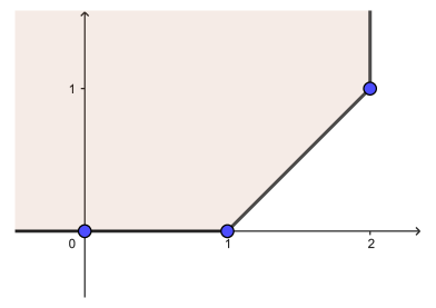
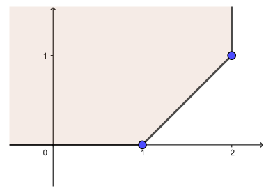
Figure 1: Newton polygon associated with $P(\partial_{z})$ in Example 1 and 2

Example 3

Let $a,b>0$. We consider the operator $P(\partial_{z}):\mathbb{C}[[z]]\to\mathbb{C}[[z]]$ given by

$$P(\partial_{z})=az+bz^{2}\partial_{z}+z^{5}\partial_{z}^{2}.$$

Its Newton polygon is represented in Figure 2 (left). We observe that $m=1$ so condition (a) in Theorem 1 does not hold, $\Lambda=\{0,1,2\}$ and $\Lambda_{m}=\{0,1\}$. It holds that $P_{-m}(\partial_{z})=az+bz^{2}\partial_{z}$ and $W_{m}(\lambda)=a+b\lambda$. Notice that $W_{m}(n)\neq 0$ for all $n\in\mathbb{N}_{0}$ so condition (b) in Theorem 1 holds. Theorem 1 guarantees that $P(\partial_{z})$ is not an automorphism of $\mathbb{C}[[z]]$. Observe there does not exist $u(z)\in\mathbb{C}[[z]]$ such that $P(\partial_{z})u(z)=1$ as $P(\partial_{z})=zP_{1}(\partial_{z})$ for some operator $P_{1}(\partial_{z})$. By direct inspection one can check that, given any element $f(z)\in z\mathbb{C}[[z]]$, there exists a unique $u(z)\in\mathbb{C}[[z]]$ such that $P(\partial_{z})u=f$.

Example 4

Let $a>0$. We consider the operator $P(\partial_{z}):\mathbb{C}[[z]]\to\mathbb{C}[[z]]$ given by

$$P(\partial_{z})=az+z^{3}\partial_{z}.$$

Its Newton polygon is represented in Figure 2 (right). We observe that $m=1$ so condition (a) in Theorem 1 does not hold, $\Lambda=\{0,1\}$ and $\Lambda_{m}=\{0\}$. It holds that $P_{-m}(\partial_{z})=az$ and $W_{m}(\lambda)=a\lambda$. Notice that $W_{m}(0)=0$ so condition (b) in Theorem 1 does not hold either. Theorem 1 guarantees that $P(\partial_{z})$ is not an automorphism of $\mathbb{C}[[z]]$.

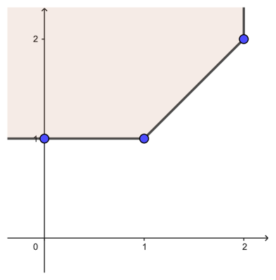
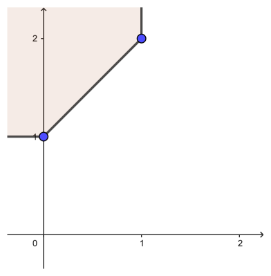
Figure 2: Newton polygon associated with $P(\partial_{z})$ in Example 3 and 4

Remark: In view of (7), the condition (a) in Theorem 1 means that the principal part of the operator $P(\partial_{z})$ defined by (4) and (5) is a Fuchsian operator given by

$$P_{0}(\partial_{z})=\sum_{j\in\Lambda_{0}}a_{j,j}z^{j}\partial_{z}^{j}.$$

Remark: Observe that Theorem 1 remains valid when replacing $a_{j}(z)\in\mathcal{O}(D)$ in (5) by $a_{j}(z)\in\mathbb{C}[[z]]$ for $j\in\Lambda$. A detailed study on the convergence will be made precise in Section 3.2, when taking $s=0$.

3.1 Linear automorphisms. The moment differential operator setting

Theorem 1 can be generalized to the more general framework of moment derivatives after minor adaptations. The importance of moment derivatives in practice motivates separating the result in a single subsection, although little details will be given, except at the points in which the argument of the proof of Theorem 1 differs.

The concept of moment differentiation was put forward by W. Balser and M. Yoshino in [4], as a generalization of the classical derivation operator.

Definition 4

Let $\mathfrak{m}=(m_{n})_{n\geq 0}$ be a sequence of positive real numbers. The moment derivative operator $\partial_{\mathfrak{m},z}:\mathbb{C}[[z]]\to\mathbb{C}[[z]]$ is given by

$$\partial_{\mathfrak{m},z}\left(\sum_{n=0}^{\infty}\frac{a_{n}}{m_{n}}z^{n}\right)=\sum_{n=0}^{\infty}\frac{a_{n+1}}{m_{n}}z^{n}.$$

It is known as the moment differential operator due to the fact that sequence $\mathfrak{m}$ is usually assumed to be a sequence of moments associated with some measure. For example, the classical formal derivative is retrieved when considering $\mathfrak{m}$ to be the sequence $(n!)_{n\geq 0}$, and moment derivative is quite related to Caputo fractional differential operator when choosing the sequence $\mathfrak{m}$ as $\Gamma_{1/k}:=(\Gamma(1+\frac{n}{k}))_{n\geq 0}$, for some fixed $k>0$. Indeed, if one considers Caputo $1/k$-fractional differential operator ${}^{C}D_{z}^{1/k}$, one has that

$$(\partial_{\Gamma_{1/k},z}f)(z^{1/k})={}^{C}D_{z}^{1/k}(f(z^{1/k})),$$

for every $f\in\mathbb{C}[[z]]$. In all the previous cases, the sequence $\mathfrak{m}$ considered is a sequence of moments. Indeed, one has

$$\Gamma\left(1+\frac{p}{k}\right)=\int_{0}^{\infty}s^{p}ks^{k}e^{-s^{k}}ds,\qquad p\in\mathbb{N}_{0}.$$

A general setting embracing the previous particularizations is that of sequences of moments associated with pairs of kernel functions for generalized summability, developed by J. Sanz in [21]. The construction of Laplace-like operators via the existence of kernel functions is applied in the solution of moment differential equations, see [5, 6].

There are other sequences of great importance in applications which are quite related with moment sequences. This is the case of the $q-$factorial sequence $\Gamma_{1;q}:=([n]_{q}!)_{n\geq 0}$, for some fixed $q\in\mathbb{R}_{+}\setminus\{1\}$. This sequence is given by $[0]_{q}!=1$ and $[n]_{q}!=[n]_{q}\cdot[n-1]_{q}\cdot\ldots\cdot[1]_{q}$ for any positive integer $n$, where $[j]_{q}$ stands for the $q-$number $[j]_{q}=\sum_{h=0}^{j-1}q^{h}$. The $q-$derivative, defined by

$$D_{q,z}f(z)=\frac{f(qz)-f(z)}{qz-z},$$

for every $f\in\mathbb{C}[[z]]$ coincides with the moment derivative $\partial_{\Gamma_{1;q},z}$. When $q>1$, the sequence $\Gamma_{1;q}$ is close to the sequence of moments $(q^{\frac{n(n-1)}{2}})_{n\geq 0}$, associated with the Laplace-like operators of kernel $s\mapsto\sqrt{2\pi\ln(q)}\exp\left(\frac{\ln^{2}(\sqrt{q}s)}{2\ln(q)}\right)$ and also to a kernel involving Jacobi Theta function $s\mapsto\Theta_{1/q}(s)=\sum_{n\in\mathbb{Z}}\frac{1}{q^{\frac{n(n-1)}{2}}}s^{n}$. Both operators appear in the theory of summability of formal solutions to $q-$difference equations, see [26, 27].

In principle, $\partial_{\mathfrak{m},z}$ is only defined on formal power series, and consequently on analytic functions near some point by identification of the function with its Taylor expansion at that point. In [7, 10], the domain of $\partial_{\mathfrak{m}}$ has been extended to analytic functions defined on sectors of the complex plane which represent the sum or multisum of a formal asymptotic expansion at the vertex of the sector.

The formal nature of Theorem 1 allows to adapt the arguments of its proof when considering an operator $P(\partial_{\mathfrak{m}})$, $\mathfrak{m}=(m_{n})_{n\geq 0}$ being any sequence of positive real numbers normalized by $m_{0}=1$.

In the following results, we write $\partial_{\mathfrak{m}}$ instead of $\partial_{\mathfrak{m},z}$ for simplicity, and we assume $P(\partial_{\mathfrak{m}})$ is defined by

$$P(\partial_{\mathfrak{m}})=\sum_{j\in\Lambda}a_{j}(z)\partial_{\mathfrak{m}}^{j}.$$

Here, $\Lambda\subseteq\mathbb{N}_{0}$ is a finite set, $a_{j}$ is an analytic function on some neighborhood of the origin (or a formal power series in $z$) for all $j\in\Lambda$ of the form (5). We write $\partial_{\mathfrak{m}}^{0}=\hbox{Id}$, $\partial_{\mathfrak{m}}^{1}=\partial_{\mathfrak{m}}$ and $\partial_{\mathfrak{m}}^{j+1}=\partial_{\mathfrak{m}}\circ\partial_{\mathfrak{m}}^{j}$ recursively for every $j\geq 1$. Therefore,

$$P(\partial_{\mathfrak{m}}):\mathbb{C}[[z]]\to\mathbb{C}[[z]].$$

Definition 5

The Newton polygon associated with $P(\partial_{\mathfrak{m}})$ is defined as the Newton polygon associated with $P(\partial_{z})$.

The lower ordinate of Newton polygon will still be denoted by $m$, and we preserve the definition of $\Lambda_{m}$. The generalized characteristic polynomial of $P(\partial_{\mathfrak{m}})$, denoted $W_{m,\mathfrak{m}}$ is defined by

$$W_{m,\mathfrak{m}}(\lambda)=\sum_{j\in\Lambda_{m},\ j\leq\lambda}a_{j,j+m}\frac{m_{\lambda}}{m_{\lambda-j}}.$$

Observe that $W_{m,(n!)_{n\geq 0}}(\lambda)$ coincides with $W_{m}(\lambda)$.

The proof of Theorem 1 can be mimicked to prove the following result.

Corollary 1

Let $P$ be as above and let $\mathfrak{m}=(m_{n})_{n\geq 0}$ be a sequence of positive real numbers. The operator $P(\partial_{\mathfrak{m}})$ is a linear automorphism on $\mathbb{C}[[z]]$ if and only if the following conditions hold:

• The lower ordinate of the Newton polygon $N(P)$ is equal to zero.

• (non-resonance condition) The generalized characteristic polynomial $W_{0,\mathfrak{m}}(n)$ of $P(\partial_{\mathfrak{m}})$ is different from zero for all $n\in\mathbb{N}_{0}$.

In the particular case of $\mathfrak{m}=\Gamma_{1/k}$, the operator under study is

$$P({}^{C}D_{z}^{1/k})=\sum_{j\in\Lambda}a_{j}(z^{1/k}){}^{C}D_{z}^{1/k}:\mathbb{C}[[z^{1/k}]]\to\mathbb{C}[[z^{1/k}]],$$

dealing with automorphisms of $\mathbb{C}[[z^{1/k}]]$.

Considering $\mathfrak{m}=\Lambda_{1;q}$ for some $q>1$, we deal with $P(D_{q,z}):\mathbb{C}[[z]]\to\mathbb{C}[[z]]$, with $W_{m,\Lambda_{1;q}}(\lambda)=\sum_{j\in\Lambda_{m},\ j\leq\lambda}a_{j,j+m}\prod_{h=\lambda-j+1}^{\lambda}[h]_{q}$. Observe the confluence of all the constructions under these settings to those studied in the first part of Section 3.

3.2 Linear automorphisms. Gevrey settings

In this subsection we state equivalent conditions for an automorphism $P(\partial_{z})$ of $\mathbb{C}[[z]]$ to remain an automorphism when restricted to $\mathbb{C}[[z]]_{s}$. In particular, we study the convergent case for $s=0$.

Theorem 2

Let $s\geq 0$. The operator $P(\partial_{z})$ is a linear automorphism on $\mathbb{C}[[z]]$ which extends to the automorphism on $\mathbb{C}[[z]]_{s}$ if and only if the following conditions hold:

1. The lower ordinate $m$ of the Newton polygon $N(P)$ is equal to zero.

2. (non-resonance condition) $W_{0}(n)\neq 0$ for every $n\in\mathbb{N}_{0}$.

3. The first positive slope of the Newton polygon $N(P)$ is greater or equal to $k=1/s$.

Proof The proof is based on the Gevrey Index Theorem for linear differential operators [12, Corollary 4.25] (see also [14] and [17]).

($\Rightarrow$) Since $P(\partial_{z})\colon\mathbb{C}[[z]]\to\mathbb{C}[[z]]$ is a linear automorphism, by Theorem 1 we get the assertions (a) and (b). Moreover, since $\chi(P(\partial_{z}),\mathbb{C}[[z]]_{s})=0$, by [12, Corollary 4.25] we conclude that (c) also holds.

($\Leftarrow$) If $m=0$ and $W_{0}(n)\neq 0$ for every $n\in\mathbb{N}_{0}$ then by Theorem 1 the operator $P(\partial_{z})\colon\mathbb{C}[[z]]\to\mathbb{C}[[z]]$ is a linear automorphism and, in particular, $\dim\ker(P(\partial_{z}),\mathbb{C}[[z]])=0$. Since $\mathbb{C}[[z]]_{s}\subset\mathbb{C}[[z]]$, we conclude that $\ker(P(\partial_{z}),\mathbb{C}[[z]]_{s})\subset\ker(P(\partial_{z}),\mathbb{C}[[z]])$, so also $\dim\ker(P(\partial_{z}),\mathbb{C}[[z]]_{s})=0$. If the first positive slope of the Newton polygon $N(P)$ is greater or equal to $k=1/s$, then by [12, Corollary 4.25] we see that $\chi(P(\partial_{z}),\mathbb{C}[[z]]_{s})=0$, so also $\dim\mathrm{coker}(P(\partial_{z}),\mathbb{C}[[z]]_{s})=0$. Hence $P(\partial_{z})\colon\mathbb{C}[[z]]_{s}\to\mathbb{C}[[z]]_{s}$ is a linear automorphism. $\Box$

Example 5

Recall that $P(\partial_{z})$ determines an automorphism of $\mathbb{C}[[z]]$ for $P(\partial_{z})$ given in Example 1. Theorem 2 guarantees that $P(\partial_{z})$ remains to be an automorphism of $\mathbb{C}[[z]]_{s}$ for every $s\geq 1$. This can be proved directly. Indeed, assume that $P(\partial_{z})u=f$ for some $u(z)=\sum_{n\geq 0}u_{n}z^{n}\in\mathbb{C}[[z]]$ and $f(z)=\sum_{n\geq 0}f_{n}z^{n}\in\mathbb{C}[[z]]_{s}$ for some $s\geq 0$. This entails that $|f_{n}|\leq C_{1}A_{1}^{n}\Gamma(1+sn)\leq CA^{n}n!^{s}$ for some $C_{1},C,A_{1},A>0$ by Stirling’s formula.

First assume that $s\geq 1$. Observe from the recursion formula

$$u_{n}=\frac{f_{n}-(n-1)(n-2)u_{n-1}}{a+bn},\qquad n\geq 3$$

that one can choose $\tilde{C},\tilde{A}>0$ large enough such that $|u_{0}|=|f_{0}|/a\leq\tilde{C}$, $|u_{j}|=|f_{j}|/(a+jb)\leq\tilde{C}+\tilde{A}^{j}j^{s}$ for $j=1,2$ and with $\tilde{C}\geq C$, $\tilde{A}\geq\max\left\{A,\frac{\max\{A,1\}}{\min\{a,b\}}\right\}$. One can prove by induction that

(16) $$|u_{n}|\leq\tilde{C}\tilde{A}^{n}n!^{s},\qquad n\geq 0.$$

Again, Stirling’s formula allows to conclude that $u\in\mathbb{C}[[z]]_{s}$. The estimate (16) is valid for $n=0,1,2$. Assume it is valid up to some $n-1\geq 1$. Then,

$$|u_{n}|\leq\frac{1}{a+bn}\left[|f_{n}|+(n-1)(n-2)|u_{n-1}|\right]\leq\frac{1}{a+bn}\left[CA^{n}n!^{s}+n^{2}\tilde{C}\tilde{A}^{n-1}(n-1)!^{s}\right]\\ \leq n!^{s}\frac{CA^{n}+n\tilde{C}\tilde{A}^{n-1}}{a+bn}\leq\tilde{C}\tilde{A}^{n-1}n!^{s}\frac{n+A}{\min\{a,b\}(n+1)}\leq\tilde{C}\tilde{A}^{n}n!^{s}.$$

This guarantees that $P(\partial_{z}):\mathbb{C}[[z]]_{s}\to\mathbb{C}[[z]]_{s}$ is an automorphism for $s\geq 1$. If $0<s<1$, and we consider $f(z)=\sum_{n\geq 0}n!^{s}z^{s}\in\mathbb{C}[[z]]_{s}$, one can prove in an analogous manner the existence of $\tilde{C}_{1},\tilde{A}_{1}>0$ such that $|u_{n}|\geq\tilde{C}_{1}\tilde{A}_{1}^{n}n!$, so $P(\partial_{z})$ is not an automorphism.

Taking $s=0$ in Theorem 2 we get

Corollary 2

The operator $P(\partial_{z})$ of order $p\in\mathbb{N}$ is a linear automorphism on $\mathbb{C}[[z]]$, which extends to the automorphism on $\mathbb{C}\{z\}$ if and only if the following conditions hold:

1. $N(P(\partial_{z}))=\mathbin{\vrule height=0.55974pt,depth=0.0pt,width=5.59721pt\vrule height=6.88889pt,depth=0.0pt,width=0.55974pt}\,(p,0)$,

2. (non-resonance condition) $W_{0}(n)\neq 0$ for every $n\in\mathbb{N}_{0}$.

Example 6

Example 1 describes an automorphism of $\mathbb{C}[[z]]$ which does not extend to an automorphism of $\mathbb{C}\{z\}$ in view of the Newton polygon associated with $P(\partial_{z})$. See Figure 1 (left).

Let us consider a slightly modified example.

Example 7

Let $a,b>0$. We consider the operator $P(\partial_{z}):\mathbb{C}[[z]]\to\mathbb{C}[[z]]$ given by

$$P(\partial_{z})=a+bz\partial_{z}.$$

Its Newton polygon is represented in Figure 3. We observe that $m=0$ so condition (a) in Theorem 1 applies. We observe that $W_{m}(\lambda)=a+b\lambda$ so that condition (b) in Theorem 1 holds. This entails that $P(\partial_{z})$ is an automorphism of $\mathbb{C}[[z]]$. Condition (a) of Corollary 3 also holds. Therefore, $P(\partial_{z})$ is also an automorphism of $\mathbb{C}\{z\}$.

Observe that, given $f(z)=\sum_{n\geq 0}f_{n}z^{n}\in\mathbb{C}[[z]]$, the formal power series $u(z)=\sum_{n\geq 0}u_{n}z^{n}\in\mathbb{C}[[z]]$ defined by $u_{0}=f_{0}/a$, and for all $n\geq 1$ $u_{n}=f_{n}/(a+bn)$ is the unique formal power series satisfying $P(\partial_{z})u=f$. In addition to this, if there exist $C,A>0$ such that $|f_{n}|\leq CA^{n}$, for every $n\geq 0$, i.e., $f\in\mathbb{C}\{z\}$ with radius of convergence at least $1/A$, then one has that $|u_{0}|=|f_{0}|/a\leq C/a$ and $|u_{n}|=|f_{n}|/(a+bn)\leq(C/a)A^{n}$ for every $n\geq 0$. As a consequence, $u\in\mathbb{C}\{z\}$ with radius of convergence at least $1/A$. Indeed, observe that given $f\in\mathbb{C}\{z\}$ the equation $P(\partial_{z})u=au+bz\partial_{z}u=f(z)$ is a first order linear ODE which can be solved by variation of constants formula for a concrete $f$.

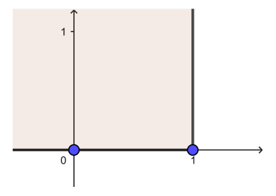
Figure 3: Newton polygon associated with $P(\partial_{z})$ in Example 5

In the last part of this section we exhibit how the properties of a differential operator can be derived from a simpler operator which maintains its most significant terms, the principal part of the differential operator. Its detection is now explained.

By (4) and (5) we may write the operator $P(\partial_{z})$ as

$$P(\partial_{z})=\sum_{(j,k)\in\Lambda\times\mathbb{N}_{0}}a_{jk}z^{k}\partial_{z}^{j}.$$

Next, for the Newton polygon $N(P)$ given by (6) we define a set of indices $\Delta\subset\Lambda\times\mathbb{N}_{0}$ as

$$\Delta:=\{(j,k)\in\Lambda\times\mathbb{N}_{0}\colon a_{jk}\neq 0,\ (j,k-j)\in\partial N(P)\}.$$

We are in position to define the principal part $P_{N}(\partial_{z})$ of the operator $P(\partial_{z})$ with respect to the Newton polygon $N(P)$ as

$$P_{N}(\partial_{z})=\sum_{(j,k)\in\Delta}a_{jk}z^{k}\partial_{z}^{j}.$$

Observe that the operators $P(\partial_{z})$ and $P_{N}(\partial_{z})$ have the same Newton polygon, the same principal part and the same characteristic polynomial. Hence by Theorems 1 and 2 we get that the operator $P(\partial_{z})$ has the same properties as the operator $P_{N}(\partial_{z})$. More precisely, we have

Corollary 3

The operator $P(\partial_{z})$ is a linear automorphism on $\mathbb{C}[[z]]$ if and only if the operator $P_{N}(\partial_{z})$ is a linear automorphism on the same space.

Moreover, for fixed $s\geq 0$ the automorphism $P(\partial_{z})$ on $\mathbb{C}[[z]]$ extends to the automorphism on $\mathbb{C}[[z]]_{s}$ if and only if the automorphism $P_{N}(\partial_{z})$ extends in the same way.

The previous result is very important in applications, allowing to simplify certain concrete problems in a significant manner. The following example shows its importance.

Example 8

Consider the differential operator

$$P(\partial_{z})=p_{1}(z)+zp_{2}(z)\partial_{z}+z^{3}\partial_{z}^{2},$$

where $p_{1},p_{2}\in\mathbb{C}[z]$ with $p_{1}(0)=a$ for some $a>0$ and $p_{1}(0)=b$ for some $b>0$. Then, $P(\partial_{z})$ is a linear automorphism on $\mathbb{C}[[z]]$ which extends to a linear automorphism on $\mathbb{C}[[z]]_{s}$ only for $s\geq 1$. This is a consequence of Example 1 and Example 5 and the fact that $P(\partial_{z})$ shares its Newton polygon with the differential operator in these examples.

4 Integro-differential operators of two variables

In this section we assume that $\Lambda$ is a finite subset of indices in $\mathbb{N}_{0}\times\mathbb{N}_{0}$. We consider a partial differential operator of the form

(17) $$P(\partial_{t},\partial_{z})=\sum_{(j,r)\in\Lambda}a_{jr}(t,z)\partial_{t}^{j}\partial_{z}^{r}\quad\textrm{with}\quad a_{jr}(t,z)=\sum_{n=\mathrm{ord}_{t}(a_{jr})}^{\infty}a_{j,r,n}(z)t^{n}\in\mathcal{O}[[t]]\ (\textrm{or}\ \mathbb{C}[[t,z]]).$$

For such operator $P(\partial_{t},\partial_{z})$ we define the Newton polygon (see [24]) as the convex hull of the union of sets $\mathbin{\vrule height=0.55974pt,depth=0.0pt,width=5.59721pt\vrule height=6.88889pt,depth=0.0pt,width=0.55974pt}\,(j+r,\mathrm{ord}_{t}(a_{jr})-j)$ for $(j,r)\in\Lambda$, namely

(18) $$N(P):=\mathrm{conv}\left\{\bigcup_{(j,r)\in\Lambda}\mathbin{\vrule height=0.55974pt,depth=0.0pt,width=5.59721pt\vrule height=6.88889pt,depth=0.0pt,width=0.55974pt}\,(j+r,\,\mathrm{ord}_{t}(a_{jr})-j)\right\}.$$

Let us recall that $\mathbin{\vrule height=0.55974pt,depth=0.0pt,width=5.59721pt\vrule height=6.88889pt,depth=0.0pt,width=0.55974pt}\,(a,b)=\{(x,y)\in\mathbb{R}^{2}\colon x\leq a,\ y\geq b\}$ denotes the second quadrant of $\mathbb{R}^{2}$ translated by the vector $(a,b)$.

In this section we assume that

$$m:=\max_{(j,r)\in\Lambda}(j-\mathrm{ord}_{t}(a_{jr}))\geq 0.$$

Observe that the initial problem

$$\left\{\begin{array}[]{l}P(\partial_{t},\partial_{z})u(t,z)=f(t,z)\\ \partial_{t}^{j}u(0,z)=\varphi_{j}(z)\quad\textrm{for}\quad j=0,\dots,m-1\end{array}\right.$$

has exactly one solution $u(t,z)\in\mathcal{O}[[t]]$ for every $f(t,z)\in\mathcal{O}[[t]]$ and $\varphi_{j}(z)\in\mathcal{O}(D)$ ($j=0,\dots,m-1$) if and only if the integro-differential operator

(19) $$P(\partial_{t},\partial_{z})\partial_{t}^{-m}\colon\mathcal{O}[[t]]\to\mathcal{O}[[t]]$$

is a linear automorphism.

For this reason in this section, we reformulate the problem to studying necessary and sufficient conditions under which the integro-differential operator (19) is a linear automorphism.

To this end we consider the principal part of the operator $P(\partial_{t},\partial_{z})$ with respect to $\partial_{t}$ given by (17), which is defined by

(20) $$P_{m}(\partial_{t},\partial_{z}):=\sum_{(j,r)\in\Lambda_{m}}a_{j,r,j-m}(z)t^{j-m}\partial_{t}^{j}\partial_{z}^{r},$$

where $\Lambda_{m}:=\{(j,r)\in\Lambda\colon j-\mathrm{ord}_{t}(a_{jr})=m\}$.

Before stating the main results of the present work, we provide some preliminary auxiliary constructions.

Since $j\geq m$ for $(j,r)\in\Lambda_{m}$, one may apply the operator (17) to the formal power series $u(t,z)=\sum_{n=0}^{\infty}u_{n}(z)t^{n}$ in $\mathcal{O}[[t]]$ (or $\mathbb{C}[[t,z]]$) to obtain that

$$P_{m}(\partial_{t},\partial_{z})\partial_{t}^{-m}\left(\sum_{n=0}^{\infty}u_{n}(z)t^{n}\right)=\\ =\sum_{n=0}^{\infty}\left(\sum_{(j,r)\in\Lambda_{m}}a_{j,r,j-m}(z)n(n-1)\cdot\ldots\cdot(n-(j-m)+1)\partial_{z}^{r}\right)u_{n}(z)t^{n}=\sum_{n=0}^{\infty}\tilde{P}_{m}(n,\partial_{z})u_{n}(z)t^{n},$$

where $a_{j,r,j-m}(z)=z^{\alpha_{j,r}}\tilde{a}_{j,r,j-m}(z)$ with $\alpha_{j,r}=\mathrm{ord}_{z}(a_{j,r,j-m}(z))$, and

(21) $$\tilde{P}_{m}(n,\partial_{z})=\sum_{(j,r)\in\Lambda_{m}}\tilde{a}_{j,r,j-m}(z)z^{\alpha_{j,r}}n(n-1)\cdot\ldots\cdot(n-(j-m)+1)\partial_{z}^{r}.$$

To construct the principal part of the above operator $\tilde{P}_{m}(n,\partial_{z})$ with respect to $\partial_{z}$, we put

$$l:=\min_{(j,r)\in\Lambda_{m}}(\alpha_{j,r}-r)\quad\textrm{and}\quad\Lambda_{m,l}:=\{(j,r)\in\Lambda_{m}\colon\alpha_{j,r}-r=l\}.$$

Then, the principal part of $\tilde{P}_{m}(n,\partial_{z})$ is given by

$$\tilde{P}_{m,-l}(n,\partial_{z})=\sum_{(j,r)\in\Lambda_{m,l}}\tilde{a}_{j,r,j-m}(z)z^{r+l}n(n-1)\cdot\ldots\cdot(n-(j-m)+1)\partial_{z}^{r}.$$

By plugging the power series $u_{n}(z)=\sum_{k=0}^{\infty}u_{nk}z^{k}$ in $\mathbb{C}[[z]]$ (or $\mathbb{C}[[z]]_{s}$ for some $s\geq 0$) into the previous operator, we arrive at

$$\tilde{P}_{m,-l}(n,\partial_{z})u_{n}(z)=\sum_{k=0}^{\infty}\sum_{(j,r)\in\Lambda_{m,l}}\tilde{a}_{j,r,j-m}(z)n(n-1)\cdot\ldots\cdot(n-(j-m)+1)k(k-1)\cdot\ldots\cdot(k-r+1)u_{nk}z^{k+l}.$$

Therefore,

$$\tilde{P}_{m,-l}(n,\partial_{z})u_{n}(z)=\sum_{k=0}^{\infty}W_{m,l}(n,k,z)u_{nk}z^{k+l},$$

where

(22) $$W_{m,l}(n,k,z)=\sum_{(j,r)\in\Lambda_{m,l}}\tilde{a}_{j,r,j-m}(z)n(n-1)\cdot\ldots\cdot(n-(j-m)+1)k(k-1)\cdot\ldots\cdot(k-r+1).$$

At this point, we are in conditions to prove the first main result of the present work.

Theorem 3

The operator $P(\partial_{t},\partial_{z})\partial_{t}^{-m}$ is a linear automorphism on $\mathbb{C}[[t,z]]$ if and only if the following conditions hold:

1. The lower ordinate $l$ of the Newton polygon $N(\tilde{P}_{m}(n,\partial_{z}))$ is equal to zero for every $n\in\mathbb{N}_{0}$,

2. (non-resonance condition) $W_{m,0}(n,k,0)\neq 0$ for every $n,k\in\mathbb{N}_{0}$.

Proof The proof is divided into two steps. In the first step, we reduce the problem to that in the one variable settings, already solved in Theorem 1. In a second step, we adapt the necessary and sufficient conditions obtained in that result to the several variable framework.

First, let us define $Q(\partial_{t},\partial_{z}):=P(\partial_{t},\partial_{z})-P_{m}(\partial_{t},\partial_{z})$, where $P_{m}(\partial_{t},\partial_{z})$, given by (20), is the principal part of the operator $P(\partial_{t},\partial_{z})$. Then the equation

$$P(\partial_{t},\partial_{z})\partial_{t}^{-m}u=f$$

for $u=\sum_{n=0}^{\infty}u_{n}(z)t^{n}$ and $f=\sum_{n=0}^{\infty}f_{n}(z)t^{n}$ can be written as

$$P_{m}(\partial_{t},\partial_{z})\partial_{t}^{-m}\left(\sum_{n=0}^{\infty}u_{n}(z)t^{n}\right)+Q(\partial_{t},\partial_{z})\partial_{t}^{-m}\left(\sum_{n=0}^{\infty}u_{n}(z)t^{n}\right)=\sum_{n=0}^{\infty}f_{n}(z)t^{n}.$$

Since $Q(\partial_{t},\partial_{z})$ is the rest of the operator $P(\partial_{t},\partial_{z})$, the lower ordinate of $N(Q)$ is greater than $-m$. Hence we can write

$$Q(\partial_{t},\partial_{z})\partial_{t}^{-m}\left(\sum_{n=0}^{\infty}u_{n}(z)t^{n}\right)=\sum_{n=1}^{\infty}\left(\sum_{k=1}^{n}\tilde{Q}(n,k,\partial_{z})u_{n-k}(z)\right)t^{n}$$

for some uniquely defined differential operators $\tilde{Q}(n,k,\partial_{z})$, where $n,k\in\mathbb{N}$ and $k\leq n$.

Since also

$$P_{m}(\partial_{t},\partial_{z})\partial_{t}^{-m}\left(\sum_{n=0}^{\infty}u_{n}(z)t^{n}\right)=\sum_{n=0}^{\infty}\tilde{P}_{m}(n,\partial_{z})u_{n}(z)t^{n},$$

where $\tilde{P}_{m}(n,\partial_{z})$ is given by (21), we conclude that

(23) $$\left\{\begin{array}[]{ll}\tilde{P}_{m}(n,\partial_{z})u_{n}(z)=f_{n}(z)&\textrm{for}\ n=0\\ \tilde{P}_{m}(n,\partial_{z})u_{n}(z)=f_{n}(z)-\sum_{k=1}^{n}\tilde{Q}(n,k,\partial_{z})u_{n-k}(z)&\textrm{for}\ n\geq 1.\end{array}\right.$$

The fact that the operator $P(\partial_{t},\partial_{z})\partial_{t}^{-m}$ is a linear automorphism on $\mathbb{C}[[t,z]]$ means that for every $f=\sum_{n=0}^{\infty}f_{n}(z)t^{n}$ in $\mathbb{C}[[t,z]]$ there exists exactly one $u=\sum_{n=0}^{\infty}u_{n}t^{n}$ in $\mathbb{C}[[t,z]]$ satisfying $P(\partial_{t},\partial_{z})\partial_{t}^{-m}u=f$. The previous statement is equivalent to the fact that for every $f_{n}(z)\in\mathbb{C}[[z]]$ and every $u_{0}(z),\dots,u_{n-1}(z)\in\mathbb{C}[[z]]$ there exists exactly one $u_{n}(z)$ in $\mathbb{C}[[z]]$ satisfying (23) for $n=0,1,2,\dots$. So it means that $\tilde{P}_{m}(n,\partial_{z})$ is a linear automorphism on $\mathbb{C}[[z]]$ for every $n\in\mathbb{N}_{0}$.

In this way we proved that the operator $P(\partial_{t},\partial_{z})\partial_{t}^{-m}$ is a linear automorphism on $\mathbb{C}[[t,z]]$ if and only if the operators $\tilde{P}_{m}(n,\partial_{z})$ are linear automorphisms on $\mathbb{C}[[z]]$ for every $n\in\mathbb{N}_{0}$.

Now we are ready to prove both implications.

($\Rightarrow$) We assume that $\tilde{P}_{m}(n,\partial_{z})$ is a linear automorphism on $\mathbb{C}[[z]]$ for every $n\in\mathbb{N}_{0}$. Hence, by Theorem 1 we conclude that the lower ordinate of the Newton polygon $N(\tilde{P}_{m}(n,\partial_{z}))$ is equal to zero and $W_{m,0}(n,k,0)\neq 0$ for every $k\in\mathbb{N}_{0}$. It holds for every $n\in\mathbb{N}_{0}$, so we get conditions (a) and (b).

($\Leftarrow$) If conditions (a) and (b) hold then by Theorem 1 operator $\tilde{P}_{m}(n,\partial_{z})$ is a linear automorphism on $\mathbb{C}[[z]]$ for every $n\in\mathbb{N}_{0}$. It means that $P(\partial_{t},\partial_{z})\partial_{t}^{-m}$ is a linear automorphism on $\mathbb{C}[[t,z]]$. $\Box$

Example 9

Let $m\geq 0$. We consider the differential operator

$$P(\partial_{t},\partial_{z})=p_{0}(t,z)\partial_{t}^{m}+p_{1}(t,z)\partial_{t}^{m+1}+p_{2}(t,z)\partial_{t}^{m+1}\partial_{z},$$

where

$$p_{0}(t,z)=a+zp_{00}(z)+\sum_{n\geq 1}p_{0n}(z)t^{n}\in\mathbb{C}[[t,z]],$$

for some $a>0$ and $p_{0n}\in\mathbb{C}[[z]]$ for all $n\geq 0$,

$$p_{1}(t,z)=(b+zp_{11}(z))t+\sum_{n\geq 2}p_{1n}(z)t^{n}\in\mathbb{C}[[t,z]],$$

with $b>0$ and $p_{1n}\in\mathbb{C}[[z]]$ for all $n\geq 1$, and

$$(c+zp_{21}(z))zt+\sum_{n\geq 2}p_{2n}(z)t^{n}\in\mathbb{C}[[t,z]],$$

with $c>0$ and $p_{2n}\in\mathbb{C}[[z]]$ for all $n\geq 1$. Observe that $\Gamma=\{(m,0),(m+1,0),(m+1,1)\}$ and $\Gamma_{m}=\Gamma$. One has that

$$\tilde{P}_{m}(n,\partial_{z})=a+zp_{00}(z)+(b+zp_{11}(z))n+(c+zp_{21}(z))n\partial_{z}.$$

If $n=0$, then $\tilde{P}_{m}(0,\partial_{z})=a$ which satisfies that $N(\tilde{P}_{m}(0,\partial_{z}))=\mathbin{\vrule height=0.55974pt,depth=0.0pt,width=5.59721pt\vrule height=6.88889pt,depth=0.0pt,width=0.55974pt}\,(0,0)$ whereas for $n\geq 1$ $N(\tilde{P}_{m}(0,\partial_{z}))=\mathbin{\vrule height=0.55974pt,depth=0.0pt,width=5.59721pt\vrule height=6.88889pt,depth=0.0pt,width=0.55974pt}\,(1,0)$. Therefore, condition (a) of Theorem 3 is satisfied. In addition to this, $l=0$ and $\Gamma_{m,0}=\Gamma$. We also have $W_{m,0}(n,k,0)=a+bn+cnk\neq 0$ for all $(n,k)\in\mathbb{N}_{0}^{2}$. Condition (b) in Theorem 3 holds, and the operator $P(\partial_{t},\partial_{z})\partial_{t}^{-m}$ is a linear automorphism on $\mathbb{C}[[t,z]]$.

Remark: The sufficient condition from Theorem 3 under which the operator $P(\partial_{t},\partial_{z})\partial_{t}^{-m}$ is a linear automorphism on the space $\mathbb{C}[[t,z]]$ one can also be found in [11, Proposition 1] in a more general setting involving nonlinear operators.

Remark: Theorem 3 remains valid when replacing $a_{jr}(t,z)\in\mathcal{O}[[t]]$ in (17) by $a_{jr}(t,z)\in\mathbb{C}[[t,z]]$ for $(j,r)\in\Lambda$.

Theorem 3 can be extended to the more general framework of Section 3.1 without difficulty. Indeed, assume that $\mathfrak{m}_{1}=(m_{1,n})_{n\geq 0}$ and $\mathfrak{m}_{2}=(m_{2,n})_{n\geq 0}$ are two sequences of positive real numbers normalized by $m_{1,0}=m_{2,0}=1$.

We define the operator $\partial_{\mathfrak{m}_{1},t}^{-1}$ as the formal inverse operator of $\partial_{\mathfrak{m}_{1},t}$, whose images do not have constant term. $\partial_{\mathfrak{m}_{1},t}^{-m}$ for $m\in\mathbb{N}_{0}$ is defined recursively in a natural way.

Let us consider a moment integro-differential operator of the form

$$P(\partial_{\mathfrak{m}_{1},t},\partial_{\mathfrak{m}_{2},z})\partial_{\mathfrak{m}_{1},t}^{-m}:\mathbb{C}[[t,z]]\to\mathbb{C}[[t,z]],$$

with $P$ as in (17) substituting classical derivatives by their corresponding moment differential operators. All the constructions can be adapted to this framework in a straightforward manner. Indeed, such construction provides

$$\tilde{P}_{m}(n,\partial_{\mathfrak{m}_{2},z})=\sum_{(j,r)\in\Lambda_{m}}\tilde{a}_{j,r,j-r}(z)z^{\alpha_{j,r}}\frac{m_{1,n}}{m_{1,n-(j-m)}}\partial_{\mathfrak{m}_{2},z}^{r}$$

as the generalization of (21), and

$$W_{m,l,\mathfrak{m}_{1},\mathfrak{m}_{2}}(\lambda_{1},\lambda_{2},z)=\sum_{\genfrac{}{}{0.0pt}{2}{(j,r)\in\Lambda_{m,l}}{j\leq\lambda_{1}+m,\,r\leq\lambda_{2}}}\tilde{a}_{j,r,j-m}(z)\frac{m_{1,\lambda_{1}}m_{2,\lambda_{2}}}{m_{1,\lambda_{1}-(j-m)}m_{2,\lambda_{2}-r}}$$

generalizing (22). Theorem 3 reads as follows in this context.

Corollary 4

The operator $P(\partial_{\mathfrak{m}_{1},t},\partial_{\mathfrak{m}_{2},z})\partial_{\mathfrak{m}_{1},t}^{-m}$ is a linear automorphism on $\mathbb{C}[[t,z]]$ if and only if the following conditions hold:

1. The lower ordinate $l$ of the Newton polygon $N(\tilde{P}_{m}(n,\partial_{\mathfrak{m}_{2},z}))$ is equal to zero for every $n\in\mathbb{N}_{0}$.

2. (non-resonance condition) $W_{m,0,\mathfrak{m}_{1},\mathfrak{m}_{2}}(n,k,0)\neq 0$ for every $n,k\in\mathbb{N}_{0}$.

At this point, the results in Section 3.2 can also be applied to achieve a result under Gevrey settings in the several variable case.

Theorem 4

Let $s\geq 0$. The operator $P(\partial_{t},\partial_{z})\partial_{t}^{-m}$ is a linear automorphism on $\mathbb{C}[[t,z]]$, which extends to an automorphism on $G_{s}[[t]]$, if and only if the following conditions hold:

1. The lower ordinate $l$ of the Newton polygon $N(\tilde{P}_{m}(n,\partial_{z}))$ is equal to zero for every $n\in\mathbb{N}_{0}$.

2. The first positive slope of the Newton polygon $N(\tilde{P}_{m}(n,\partial_{z}))$ is greater or equal to $1/s$ for every $n\in\mathbb{N}_{0}$.

3. (non-resonance condition) $W_{m,0,\mathfrak{m}_{1},\mathfrak{m}_{2}}(n,k,0)\neq 0$ for every $n,k\in\mathbb{N}_{0}$.

Proof Analogously to the proof of Theorem 3, with $\mathbb{C}[[t,z]]$ and $\mathbb{C}[[z]]$ replaced by $G_{s}[[t]]$ and $\mathbb{C}[[z]]_{s}$ respectively, and also making use of that result, we conclude that the operator $P(\partial_{t},\partial_{z})\partial_{t}^{-m}$ is a linear automorphism on $\mathbb{C}[[t,z]]$ which extends to the automorphism on $G_{s}[[t]]$ if and only if the operators $\tilde{P}_{m}(n,\partial_{z})$ are linear automorphisms on $\mathbb{C}[[z]]$ and they extend to the automorphisms on $\mathbb{C}[[z]]_{s}$ for every $n\in\mathbb{N}_{0}$.

($\Rightarrow$) It holds that $\tilde{P}_{m}(n,\partial_{z})$ is a linear automorphism on $\mathbb{C}[[z]]$, which extends to the automorphism on $\mathbb{C}[[z]]_{s}$. Hence, by Theorem 2 we conclude that the lower ordinate $l$ of the Newton polygon $N(\tilde{P}_{m}(n,\partial_{z}))$ is equal to zero and its first positive slope is greater or equal to $1/s$. We also observe that $W_{m,0,\mathfrak{m}_{1},\mathfrak{m}_{2}}(n,k,0)\neq 0$ for every $k\in\mathbb{N}_{0}$. The previous statement holds for every $n\in\mathbb{N}_{0}$, so conditions (a), (b) and (c) in the enunciate hold.

($\Leftarrow$) Assume that statements (a), (b) and (c) hold. Then, Theorem 2 guarantees that the operator $\tilde{P}_{m}(n,\partial_{z})$ is a linear automorphism on $\mathbb{C}[[z]]$, which extends to a linear automorphism on $\mathbb{C}[[z]]_{s}$ for every $n\in\mathbb{N}_{0}$. This is entails that $P(\partial_{t},\partial_{z})\partial_{t}^{-m}$ is a linear automorphism on $\mathbb{C}[[t]]$ which extends to the linear automorphism on $G_{s}[[t]]$. $\Box$

As a direct consequence of Theorem 4 with $s=0$ we get

Corollary 5

The operator $P(\partial_{t},\partial_{z})\partial_{t}^{-m}$ is a linear automorphism on $\mathbb{C}[[t,z]]$ which extends to an automorphism on $\mathcal{O}[[t]]$ if and only if the following conditions hold:

1. $N(\tilde{P}_{m}(n,\partial_{z}))=\mathbin{\vrule height=0.55974pt,depth=0.0pt,width=5.59721pt\vrule height=6.88889pt,depth=0.0pt,width=0.55974pt}\,(p_{n},0)$, where $p_{n}$ denotes the order of the operator $\tilde{P}_{m}(n,\partial_{z})$ for every $n\in\mathbb{N}_{0}$,

2. (non-resonance condition) $W_{m,0,\mathfrak{m}_{1},\mathfrak{m}_{2}}(n,k,0)\neq 0$ for every $n,k\in\mathbb{N}_{0}$.

The previous result allows to substitute a given differential operator by some other with a simpler structure, when studying whether it defines an automorphism or not. We are in position to state results in this direction as it has been done in the one variable settings in Section 3. More precisely, we depart from the partial differential operator (17) and write $P(\partial_{t},\partial_{z})$ in the form

$$P(\partial_{t},\partial_{z})=\sum_{(j,r,n)\in\Lambda\times\mathbb{N}_{0}}a_{j,r,n}(z)t^{n}\partial_{t}^{j}\partial_{z}^{r}.$$

The geometry of the Newton polygon associated with such differential operator, $N(P)$ given by (18), allows us to consider the set of indices $\Delta\subset\Lambda\times\mathbb{N}_{0}$ defined as follows:

$$\Delta:=\{(j,r,n)\in\Lambda\times\mathbb{N}_{0}\colon a_{j,r,n}(z)\not\equiv 0,\ (j+r,n-j)\in\partial N(P)\}.$$

Thus, the principal part $P_{N}(\partial_{t},\partial_{z})$ of the operator $P(\partial_{t},\partial_{z})$ with respect to the Newton polygon $N(P)$ can be defined as

$$P_{N}(\partial_{t},\partial_{z})=\sum_{(j,r,n)\in\Delta}a_{j,r,n}(z)t^{n}\partial_{t}^{j}\partial_{z}^{r}.$$

Observe that the operators $P(\partial_{t},\partial_{z})$ and $P_{N}(\partial_{t},\partial_{z})$ have the same Newton polygon, the same principal part and the same characteristic polynomial. Hence by Theorems 3 and 4 we see that the operator $P(\partial_{t},\partial_{z})$ has the same properties as the operator $P_{N}(\partial_{t},\partial_{z})$. More precisely, we arrive at the following result.

Corollary 6

The operator $P(\partial_{t},\partial_{z})\partial_{t}^{-m}$ is a linear automorphism on $\mathbb{C}[[t,z]]$ if and only if the operator $P_{N}(\partial_{t},\partial_{z})\partial_{t}^{-m}$ has the same property.

Moreover, for any fixed $s\geq 0$, the operator $P(\partial_{t},\partial_{z})\partial_{t}^{-m}$ extends to the automorphism on $G_{s}[[t]]$ if and only if the operator $P_{N}(\partial_{t},\partial_{z})\partial_{t}^{-m}$ extends to the automorphism on the same space.

Example 10

Observe that the differential operator in Example 9 can be modified by adding any number of terms of the form $a_{jr}(t,z)\partial_{t}^{j}\partial_{z}^{r}$, with $j-\hbox{ord}_{t}(a_{jr})<m$. In this situation, $\Lambda_{m}$ coincides with that in Example 9, so $m$ and $\tilde{P}_{m}(n,\partial_{z})$ are the same for both differential operators, and the conditions of Theorem 3 are also satisfied.

As a conclusion of the present work, we link our results to previous works which can be found in the literature.

Using Corollary 5 we get the known sufficient conditions under which the operator $P(\partial_{t},\partial_{z})\partial_{t}^{-m}$ is a linear automorphism on the space $\mathbb{C}[[t,z]]$ or $\mathcal{O}[[t]]$. A first example is the following, dealing with operators one can find in [2, Proposition 1.1], [18, Theorem 1] or [19, Theorem 1].

Corollary 7

Let $(m,-m)$ be a vertex of $N(P)$ (i.e. $\Lambda_{m}=\{(m,0)\}$, $\mathrm{ord}_{t}(a_{m,0})=0$ and $P_{m}(\partial_{t},\partial_{z})=a_{m,0,0}(z)\partial_{t}^{m}$) and assume the non-resonance condition $a_{m,0,0}(0)\neq 0$ holds. Then, the operator $P(\partial_{t},\partial_{z})\partial_{t}^{-m}$ is a linear automorphism on $\mathcal{O}[[t]]$.

More generally we have the following result. This type of results are also studied in [3, Theorem 1].

Corollary 8

Let $\Lambda_{m}\subset\mathbb{N}_{0}\times\{0\}$ (i.e. $P_{m}(\partial_{t},\partial_{z})=\sum_{(j,0)\in\Lambda_{m}}a_{j,0,j-m}(z)t^{j-m}\partial_{t}^{j}$) such that its associated characteristic polynomial

$$W(\lambda,z):=\sum_{(j,0)\in\Lambda_{m}}a_{j,0,j-m}(z)\lambda(\lambda-1)\cdots\dots\cdot(\lambda-(j-m)+1)$$

satisfies the non-resonance condition $W(n,0)\neq 0$ for every $n\in\mathbb{N}_{0}$. Then, the Fuchsian operator $P(\partial_{t},\partial_{z})\partial_{t}^{-m}$ is a linear automorphism on $\mathcal{O}[[t]]$.

References

[1] W. Balser, Formal power series and linear systems of meromorphic ordinary differential equations. Universitext. Springer-Verlag, New York, 2000. xviii+299 pp.
[2] W. Balser, M. Loday-Richaud, Summability of solutions of the heat equation with inhomogeneous thermal conductivity in two variables. Adv. Dyn. Syst. Appl. 4 (2009), no. 2, 159–177.
[3] M. S. Baouendi, C. Goulaouic, Cauchy Problems with Characteristic Initial Hypersurface, Comm. Pure Appl. Math. 26 (1973), 455–475.
[4] W. Balser, M. Yoshino, Gevrey order of formal power series solutions of inhomogeneous partial differential equations with constant coefficients. Funkcial. Ekvac. 53 (2010), 411–434.
[5] J. Jiménez-Garrido, S. Kamimoto, A. Lastra, J. Sanz, Multisummability in Carleman ultraholomorphic classes by means of nonzero proximate orders, J. Math. Anal. Appl. 472, No. 1 (2019), 627–686.
[6] A. Lastra, S. Malek, J. Sanz, Summability in general Carleman ultraholomorphic classes. J. Math. Anal. Appl. 430 (2015), 1175–1206.
[7] A. Lastra, S. Michalik, M. Suwińska, Summability of formal solutions for some generalized moment partial differential equations, Result. Math. 76, No. 1 (2021), Paper No. 22.
[8] A. Lastra, S. Michalik, M. Suwińska, Estimates of formal solutions for some generalized moment partial differential equations, J. Math. Anal. Appl. 500 (2021), Paper No. 125094.
[9] A. Lastra, S. Michalik, M. Suwińska, Summability of formal solutions for a family of generalized moment integro-differential equations, Fract. Calc. Appl. Anal. 24 (2021), 1445–1476.
[10] A. Lastra, S. Michalik, M. Suwińska, Multisummability of formal solutions ofr a family of generalized singularly perturbed moment differential equations, Result. Math. 78, No. 2 (2023), Paper No. 49.
[11] A. Lastra, H. Tahara, Maillet type theorem for nonlinear totally characteristic partial differential equations, Mathematische Annalen 377 (2020), 1603–1641.
[12] M. Loday-Richaud, Divergent series, summability and resurgence. II. Simple and multiple summability. Lecture Notes in Mathematics, 2154. Springer, 2016.
[13] S. Malek, Double-scale Gevrey asymptotics for logarithmic type solutions to singularly perturbed linear initial value problems, Result. Math. 77, No. 5 (2022), Paper No. 198.
[14] B. Malgrange, Sur les points singuliers des équations différentielles, Enseign. Math., II. Sér. 20 (1974) , 147–176.
[15] S. Michalik, Summability of formal solutions of linear partial differential equations with divergent initial data, J. Math. Anal. Appl. 406 (2013), 243–260.
[16] S. Michalik, Analytic and summable solutions of inhomogeneous moment partial differential equations, Funkc. Ekvacioj, Ser. Int. 60, No. 3 (2017), 325–351.
[17] J.-P. Ramis, Théorèmes d’indices Gevrey pour les équations différentielles ordinaires, Mem. Am. Math. Soc. 296 (1984), 95 p.
[18] P. Remy, Gevrey order and summability of formal series solutions of some classes of inhomogeneous linear partial differential equations with variable coefficients, J. Dyn. Control Syst. 22 (2016), 693–711.
[19] P. Remy, Gevrey order and summability of formal series solutions of certain classes of inhomogeneous linear integro-differential equations with variable coefficients, J. Dyn. Control Syst. 23 (2017), 853–878.
[20] P. Remy, Summability of the formal power series solutions of a certain class of inhomogeneous nonlinear partial differential equations with a single level, J. Differential Equations 313 (2022), 450–502.
[21] J. Sanz, Flat functions in Carleman ultraholomorphic classes via proximate orders, J. Math. Anal. Appl. 415(2) (2014), 623–643.
[22] A. Shirai, Maillet type theorem for singular first order nonlinear partial differential equations of totally characteristic type. II, Opusc. Math. 35, No. 5 (2015), 689–712.
[23] M. Suwińska, Gevrey estimates of formal solutions for certain moment partial differential equations with variable coefficients, J. Dyn. Control Syst. 27, No. 2 (2021), 355–370.
[24] A. Yonemura, Newton polygons and formal Gevrey classes, Publ. RIMS Kyoto Univ. 26 (1990), 197–204.
[25] M. Yoshino, Analytic continuation of Borel sum of formal solution of semilinear partial differential equation, Asymptotic Anal. 92, No. 1–2, (2015), 65–84.
[26] C. Zhang, Développements asymptotiques -Gevrey et séries
-sommables, Annales de l’Institut Fourier, Volume 49 (1999) no. 1, 227–261.
[27] C. Zhang, Transformations de Borel-Laplace au moyen de la fonction thêta de Jacobi. C. R. Acad. Sci. Paris, t. 331, Série 1 (2000) 31–34.