A Qualitative Analysis of Common Practices in Annotations: A Taxonomy and Design Space

Abstract

Annotations are a vital component of data externalization and collaborative analysis, directing readers’ attention to important visual elements. Therefore, it is crucial to understand their design space for effectively annotating visualizations. However, despite their widespread use in visualization, we have identified a lack of a design space for common practices for annotations. In this paper, we present two studies that explore how people annotate visualizations to support effective communication. In the first study, we evaluate how visualization students annotate bar charts when answering high-level questions about the data. Qualitative coding of the resulting annotations generates a taxonomy comprising enclosure, connector, text, mark, and color, revealing how people leverage different visual elements to communicate critical information. We then extend our taxonomy by performing thematic coding on a diverse range of real-world annotated charts, adding trend and geometric annotations to the taxonomy. We then combine the results of these studies into a design space of annotations that focuses on the key elements driving the design choices available when annotating a chart, providing a reference guide for using annotations to communicate insights from visualizations.

blackOliveGreen4pt

blackOliveGreen4pt

blackOliveGreen4pt

(a)

(b)

(c)

blackOliveGreen4pt

blackOliveGreen4pt

blackOliveGreen4pt

(d)

(e)

(f)

Examples of annotated charts collected from the internet. They include, (a) the bar chart that has text, connector, and enclosure annotations to highlight differences between years; (b) the node-link diagram that has a geometric annotation to highlight the area of interest; (c) the line chart that has text, connector, and color annotations to emphasize key events; (d) the scatterplot that has text, connector, trend, and enclosure annotations to highlight and differentiate trends in the data; (e) the map has connector and text annotations highlighting key events on the journey and critiquing the visualization; and (f) the pie chart has text enumerating the exact values and color and geometric annotations emphasizing the lacrosse slice.

Introduction

Annotations play a crucial role in visualizations by emphasizing key data features, enabling viewers to comprehend and analyze information more clearly. Past study has shown that annotations in visualizations help viewers’ mental organization [4]. Additionally, annotation has been identified as one of the “critical tasks that enable iterative visual analysis” [13, 50]. However, despite the widespread use of annotations in visualizations, we lack a clear understanding of the design space of annotations. This leads to our main research questions, what are the encodings someone might annotate a visualization with, and what are the common practices for annotating different charts?

To better understand the design space available for annotating a visualization, we conducted a two-part study. First, we performed an observational study to investigate the forms of annotations used by undergraduate and graduate visualization students when prompted with high-level questions about the data to build an initial taxonomy of annotations. We provided students with three grouped bar chart visualizations, each with four high-level questions. We asked students to annotate the bar charts to make the questions as easy as possible to answer. The goal of this activity was ideation, i.e., we wanted students to creatively explore the space of possible annotation types so that we could later extract the breadth of options available. We used open-coding to summarize the resulting annotated visualizations and developed a taxonomy of bar chart annotations based on the results that included five primary annotation types: enclosures, connectors, text, marks, and color.

Our second study sought to expand upon our initial taxonomy by observing how annotations are used on diverse chart types in real-world scenarios. To accomplish this objective, we collected nearly 2,000 annotated chart images (e.g., annotated images of bar charts, line charts, scatterplots, etc.) from Google Images. A Qualitative Analysis of Common Practices in Annotations: A Taxonomy and Design Space illustrates several examples of the annotated charts we obtained. Thematic coding was applied to discern patterns in annotation usage using our prior taxonomy as a starting point. Upon the completed analysis of our images, we found that enclosures, connectors, text, marks, and color were frequently used to annotate many types of charts. We further extended our initial taxonomy by incorporating two new annotation types, namely trends and geometric annotations.

Finally, we further synthesized the results of these studies into a design space for annotating visualizations that considers how several factors work together to produce effective annotations. First, we categorized annotations into three distinct categories based on how the data used to generate them originated (e.g., directly from the data itself, derived from the data, or external knowledge brought by the user). Next, we consider the kinds of analytical tasks annotations support. Then, the design space enumerates the most commonly used annotation/visualization combinations. Finally, we discuss the use of ensembles of annotations, i.e., multiple annotations used in conjunction, when a single annotation type proved insufficient (e.g., connectors and text were frequently used together to reduce clutter). Our results offer significant insights for practitioners in data visualization into the types of annotations used in different chart types and provide a standardized framework for annotating visualizations, enabling them to explore the space of possible annotation types and incorporate new techniques into their work. This can lead to better user engagement, understanding, and decision-making across various domains that utilize visualization.

The contributions of this research are:

• We describe two observational studies of visualization students and annotation usage on a variety of chart types obtained from Google Images covering a wide range of common annotation practices.

• We developed a taxonomy of annotation types that can be used to create a more standardized and consistent approach to annotating visualizations, thereby improving their usability and usefulness.

• We propose design space for annotations that includes common practices for annotation data sources, annotation task support, annotations/visualization pairings, and annotation ensembles.

1 Prior Work

Annotations draw attention to critical parts of visualization to help externalize and explore data [21, 41, 29, 42] and facilitate collaborative data analysis [37, 5, 6, 29, 18]. Previous research has explored the use of annotation in specific contexts, such as storytelling [36] and bar charts [34]. However, there is a lack of systematic investigation into the common practices for annotating various chart types, despite the widespread use of annotations to enhance data comprehension.

1.1 Externalization, Communication, and Collaboration

Annotations serve as a vital part of externalizing an analyst’s thought process, allowing them to highlight important facts about the data in a visualization [21]. For example, annotations play a pivotal role in making sense of data and help with meta-analysis and data externalization [50]. Creating annotations can also be one of the most critical steps analysts perform in exploratory data analysis. For example, VisInReport, a visual analysis tool for insight report generation from discourse transcripts, uses annotations in different views (e.g., text, brackets, arrows, etc.) to clarify events [41]. They found that annotation played a crucial role in the reports—participants mentioned that it was impossible to include all aspects of the data without the annotations.

Borkin et al. found that adding captions and annotated text to charts could effectively communicate visual information by conducting eye-movement studies and employing experimental cognitive techniques [2]. Stokes et al. conducted empirical studies investigating the impact of text on visualizations and discovered that readers prefer a combination of text and charts and that the selection of semantic content and the placement of annotations significantly affect readers’ comprehension and interpretation. As a result, the authors recommend guidelines to help readers determine the appropriate type and placement of content for an intended message [45]. Ottley et al. investigated whether combining text and visualization improves users’ understanding of complex information by studying eye-tracking patterns in a Bayesian reasoning problem. The results suggest that users do not integrate information across the two representations and primarily rely on text [33]. Marshall et al. studied personal and shared annotations made while reading digital materials by comparing students’ annotations and those shared online. They found that few personal annotations were shared, and the shared annotations underwent significant changes [30].

Annotation can also help in collaborative analysis by externalizing the analyst’s thoughts to share with collaborators [37]. Vogt et al. explored the impact of collaborative visual analytics on intelligence analysis through a shared workspace with high-resolution displays [48], where annotations of different forms could potentially assist the team in organizing and comprehending the information, thus enhancing their analytical capabilities. Mahyar et al. emphasized that annotations and notes are crucial in supporting discussions, exploratory visual data analysis, and linking the system with an analyst’s cognitive processes [29]. Chen et al. discussed the importance of facilitating annotations in Asynchronous Collaborative Visual Analysis to establish common ground so that the insights from the individual work can be used to develop a shared understanding [5]. With their tool Click2Annotate [6], they demonstrated that annotations of insights in the data could capture patterns (e.g., clusters and outliers) with higher semantic richness over actions and events. In addition, an analytical study of intelligence analysis practices found that annotations were frequently used to understand the data’s facts or events in various forms (e.g., pens, highlighters, etc.).

Since sketching tools that support annotations may assist in such data analysis, annotation tools should facilitate collaborative data analysis [8]. Ellis et al. described a system that enabled collaborative annotation of visual data using digital ink on tablets, called CAV, which stores data and annotations as separate layers to provide a natural mechanism to annotate visual displays and extends remote collaboration on visual data by publishing visualizations as streams of images [11]. Finally, the UberTagger tool provided a comment panel where users could use comments as annotations or tags to highlight any event or issue and communicate them to the other members of the team [3, 43].

These studies demonstrate that annotations have a valuable contribution to make to the data analysis process, and a clearer understanding of their design space will make their usage more effective.

1.2 Annotation Techniques

People leverage a wide range of visual marks to annotate data. Kong et al. suggested that annotations function as external cues, which can be utilized to highlight the focal point in visualizations by adding supplementary elements like text, arrows, rectangles, brackets, etc. [22]. They introduced graphical overlays, visual elements that are layered onto charts, such as reference structures (e.g., gridlines), highlights (e.g., outlines around important marks), redundant encodings (e.g., numerical data labels), summary statistics (e.g., min or max), and annotations (e.g., descriptive text) [24]. They showed that graphical overlays help readers with several tasks. Additionally, they proposed an automated method for applying graphic overlays to existing charts. Chen et al. presented a technique and working prototype called TouchtoAnnotate, where people can create annotations in a multi-touch interface with “typing free” annotations that required very little human effort [7].

Free-form ink annotations (e.g., circles, lines, arrows, etc.) and text highlight the visually salient perceptual features (e.g., peaks, valleys, rising slopes, declining slopes, etc.) during asynchronous collaborations [23]. Latif et al. introduced a framework for contextual linking of text and interactive graphics, including sparklines, using specific markups to produce interactive web documents, and integrating text, sparklines, and large-scale figures into one coherent unit [26]. Hopkins et al. proposed Visualint, a technique for expressing chart construction errors to a lay audience that provides a general design language with sketchy, hand-drawn annotations and annotations for additional context to facilitate the identification of errors without interfering with chart reading [15] In another study, annotations on bar charts, specifically trends in bar heights and text values on bars, were used to optimize the visualization’s layout by utilizing an area of interest measure [35]. There is a great deal of overlap in the methods used to encode annotations by all of these prior works. Their focus has, by and large, been on technical methods of applying annotations to visualization. None has thoroughly evaluated the design space of annotations themselves.

1.3 Applications Utilizing Annotation

Many applications have allowed users to apply annotations as a software feature. For example, although not a focus of the original design, an evaluation of Jigsaw [44], a comprehensive tool that helps with sense-making during investigative analysis, demonstrated how it facilitated annotations [20]. CzSaw, a visual analytics tool that features a history navigation channel and multiple visual representations to assist analysts in understanding, exploring, referencing, and reusing their analysis process, supports analysts using annotations to document their decision-making process [19]. Heer et al. enabled users to employ graphical annotations in their website called sense.us for collaborative data analysis using interactive visualizations. Sense.us emphasized that graphical annotations can promote social interaction and sensemaking around visualized data by enabling users to contribute contextual knowledge, deepen understanding, and build consensus through discussion and feedback [14]. Similarly, Viegas et al. provided analysts with the ability to associate freeform textual and graphical annotations in interactive visualizations [47]. Arlene et al. demonstrated an application of annotations through a tool that detects deception (e.g., truncated y-axis, inverted y-axis, aspect ratio distortion, etc.) in line charts [12].

Finally, annotations are also a key element of data-driven storytelling, where the annotations help to focus the viewer’s attention on the data that supports critical narrative elements [40, 28, 25, 16, 38]. ChartAccent is a tool that facilitates people to create annotations for data-driven storytelling by choosing from a palette of annotations [36]. The authors designed the space for chart annotations by exploring 106 professional charts. In their paper, the authors argue that we should better understand the annotation design space: the annotation types, the purposes of the annotations, and how they are applied to charts. The tool, Contextifier, provides context to a news article about a company by providing annotated line graphs of stock performance. The focus was on generating additive context messages and identifying visually salient data [17]. Chun et al. investigated the impact of annotations on news data visualizations. They carried out perception tests to measure the variations in information retention among readers exposed to different forms of annotations [9].

Apart from all of these prior investigations of annotations, our work introduces a new design space of annotations, focus explicitly on common practices in a wide variety of chart types. Such a design space forms an important foundation for codifying the best practice for annotating graphics to improve their readability.

2 A Taxonomy and Design Space of Annotations

Annotations are crucial to understanding visualizations and effectively communicating the underlying data. Therefore, it is necessary to understand the design space for annotations by exploring the common practices for annotations. Given all we learned from prior work, we found that even the definition of what, in general, qualified as an annotation was ambiguous. We settled upon the following definition, which is utilized throughout both studies for determining if a mark is an annotation.

Annotations are supplementary elements, such as graphical shapes, text, or color, added to a visualization to provide additional context beyond the basic data presented, and to draw attention to specific portions or elements of the data, thereby enhancing the understandability and expressiveness of the visualization.

We now describe our two-part study, to develop a taxonomy and design space of common annotation practices.

3 Study 1: Visualization Student Annotations

We conducted an initial study to understand how people annotate bar charts when prompted with specific questions about the data with the goal of developing a taxonomy of common practices. To do this, we utilized and analyzed a course assignment in a mixed undergraduate and graduate data visualization course.

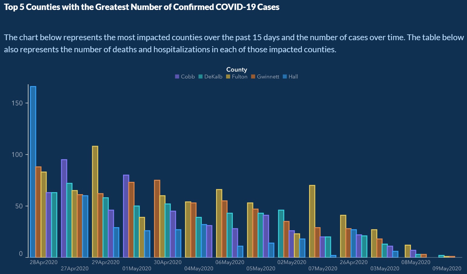
Figure 1: The viral visualization created by the Georgia Department of Public Health (GDPH) shows the number of COVID-19 cases in different counties of Georgia, but its unorthodox non-chronological arrangement of bars from highest-to-lowest on the x-axis drew public criticism.

3.1 Study Procedure

For our study, the assignment was presented to students in conjunction with a lecture on potentially deceptive practices in visualization.

The experiment itself began with a brief in-class discussion (10-15 minutes) about the Georgia Department of Public Health (GDPH) visualization that became a viral sensation in 2020 for its misleading nature (see Figure 1) [10]. The grouped bar chart was seen as deceptive for its unorthodox ordering of bars, ordered highest-to-lowest instead of chronologically. While clear labeling of the graphic can, in general, help to overcome such issues [46], the GDPH labeling failed to draw the viewer’s attention to their unorthodox ordering.

We then verbally reviewed the written assignment instructions and answered any questions. Students had seven days to complete the assignment individually, which was done outside of class. They were free to choose whatever tools they felt they needed to complete the task.

3.2 Assignment

Each assignment had three bar charts based on the GDPH visualization, each with four high-level questions (12 questions in total). For each question in the assignment, subjects were asked to: 1) identify low-level analysis tasks used to answer the high-level question and 2) annotate the visualization to make answering that question easier. A sample assignment is available in the supplemental materials.

3.2.1 Datasets and Visualizations

We wanted each student to have different data but similar trends within the data. Therefore, the datasets were generated using a random number for each county from the GDPH visualization from April 26 to May 9. We ensured that each random number fell within a specific range, e.g., for Fulton on May 4, the range was set to $[33,56]$. We used Vega-Lite [39] to create the grouped bar charts from the generated data. As with the GDPH visualization, we had five bars, one per county, of different colors for each day from April 26 to May 9. We used two variants of the x-axis, one non-chronological (like the viral GDPH visualization in Figure 1) and one chronological (like the corrected GDPH visualization, not shown). In total, we generated 150 bar charts, half chronological and half non-chronological. We built 40 unique assignments of three bar charts each. Half had two bar charts with chronological dates, one with non-chronological dates, whereas the other half had two bar charts with non-chronological dates and one with chronological dates.

3.2.2 High-Level Questions

Students were asked four types of questions about the data in the charts:

• finding a specific value (e.g., how many COVID cases are there in Hall County on May 5?);

• filtering some values from others (e.g., which counties have fewer than 40 cases of COVID on May 1?);

• aggregating (e.g., how many total COVID cases does Dekalb County have from May 1 to May 4?); and

• sorting (e.g., sort the counties in descending order based on the number of COVID cases on May 8).

3.2.3 Subject Tasks

Each high-level question required subjects to perform two activities.

Low-Level Analysis Task Identification

We developed the high-level questions so that the students could answer them by performing one or more low-level analysis tasks. We used Amar et al.’s low-level analysis task taxonomy, which enumerated ten tasks people frequently use to understand data in visualizations [1]. From that set, we selected five that fit into our study, including: retrieve a value (RV), filter, compute a derived value (CDV), find extremum (FE), and sort. Students were asked to enumerate which of these low-level analysis tasks were used to answer each of the high-level questions.

Annotating the Visualization

We instructed the students to annotate the charts in a way that made the questions as easy as possible to determine without necessarily writing the answer on the visualization. Students were allowed to annotate by hand or on the computer using whatever tools they preferred. The only instruction was that they were not to collaborate with any classmates.

3.3 Participants & Data Collected

The participants are the students from <placeholder> course that one of the authors taught at <placeholder> in Spring 2022. The course was a cross-listed elective for senior-level undergraduate and Master’s- and Ph.D.-level graduate students, with 39 students (21 undergraduate and 18 graduate). The assignment was given approximately halfway through the semester. Up to that point, the class had covered the foundations of visualization (e.g., data abstraction, visual encoding, perception, etc.). No lecture had a specific focus on bar charts or annotations.

A total of 38 students completed the study assignment. Once received, all submissions were anonymized, assigned a random number, and had quality checks performed. Our evaluation includes 20 submissions and excludes 18 submissions from the analysis (13 had no annotations, and five had minimal annotations). One student annotated only two of the three charts, but their work was included in the evaluation. Anonymized submissions are included in our osf supplement.

3.4 Data Coding

Individual Annotations

To evaluate and summarize the submitted assignments, two co-authors went through all the annotated charts and hand-coded them using an open-coding approach in several iterations. In the first iteration, they separately identified a set of annotation types based on the shapes, colors, and text used by the participants in their submissions. We linked the low-level analysis tasks performed by the participants and the associated annotations by carefully examining the submissions. Next, all authors discussed their findings and agreed on an initial taxonomy of annotation types. In the second and subsequent iterations, the two coding co-authors independently revisited each submitted assignment, re-categorizing the annotations, and the group revised the taxonomy. The process continued until a complete consensus was reached on the taxonomy and coding of individual assignments.

Ensemble Annotations

While coding the individual annotations, we began to notice that the participants frequently used multiple annotation types together when either the task was too challenging for an individual annotation or when the visualization was too cluttered to fit an annotation. Therefore, after coding the individual annotations, we engaged in several additional iterations of coding for these annotation ensembles. We followed a similar procedure, where two coding co-authors individually identified ensembles. Then, all authors discussed the findings and agreed upon a taxonomy in an iterative process that was repeated until a consensus was reached. The results of this evaluation are discussed in the Design Space of Annotations (see section 5).

Table 1: Study 1 two-level taxonomy of annotations with the frequency for tasks. Box colors indicate frequency: 1-9 10-19 20+.

3.5 Initial Taxonomy of Annotations

We identified 14 annotation types which were grouped into five top-level annotation categories, namely: Enclosure, Connector, Text, Mark, and Color. The two-level taxonomy, along with the frequency of usage of annotations, can be found in Table 1.

Enclosure

Enclosure is an annotation that uses a partially or fully closed boundary, including the ellipse, bracket, half-box, and rectangle categories. The enclosure annotations were used in a variety of situations. For example, in LABEL:fig:example1, rectangles are used for filtering the number of cases in Fulton county on May 1. Similarly, in LABEL:fig:example2, ellipses are used for the filtering, half-boxes were used to support the filtering, and a rectangle is used for a sorting task. Brackets were used to mark the range indicating the bar/axes in LABEL:fig:example2 from April 27 to May 2. Enclosure was generally used for RV and filter tasks and CDV and FE tasks to a lesser extent. Overall, ellipse and rectangle annotations were used most frequently.

Connector

A connector is an annotation that uses a line (e.g., solid, dotted, or directional line), which includes arrow (directional) and line (undirected) categories. Line annotations were used, e.g., to mark the height of a bar relative to the axis or to represent the trend in the height of bars (see LABEL:fig:example3). Similarly, arrow annotations were used for pointing text to a particular bar or group of bars (see LABEL:fig:example3) or to point the enclosure annotation to a bar, axis-value, or legend, or vice-versa. Students used connector annotations for RV, filter, and, to a lesser extent, FE and sorting tasks. Notably, most of the time, connectors did not appear alone but were combined with other annotations (i.e., into ensembles) for a given task.

Text

Text is an annotation that uses words or sentences to answer questions about the data, with second-level categories of descriptions, values, and legends. Description annotations describes a process, information, computation, or derivation that supports a particular task annotation, e.g., in LABEL:fig:example1, where the text “Hall has the highest cases on May 5.” Value annotations are text used to highlight the exact data, e.g., in LABEL:fig:example2 and LABEL:fig:example3, where a number is used to represent the bar length. Legend annotation was used for any labels on legends, e.g., the text enclosed in the colored boxes in LABEL:fig:example1 or annotating the trend in a number of cases in Hall County in LABEL:fig:example3. From Table 1, description-based text annotations were broadly applied for all five tasks. Text enumerating values was used frequently for RV tasks. Finally, legend text was frequently used for filter tasks. Overall, we observed that text annotations were commonly used for elaborating on what other annotations were highlighting and as a last resort when no other annotations were suitable.

Mark

Marks are annotations that use symbols or shapes to answer questions about data, which perform the function of identifying a particular object or category (e.g., a county or date). For example, in LABEL:fig:example5, different marks (i.e., i, ii, iii, etc.) were used to denote the question numbers. In the same submission, circular and T-shaped marks were used to denote different dates. Further, marks were always accompanied by color for differentiating the marks, which is captured by the color category. From Table 1, mark-based annotations were primarily used for filter tasks.

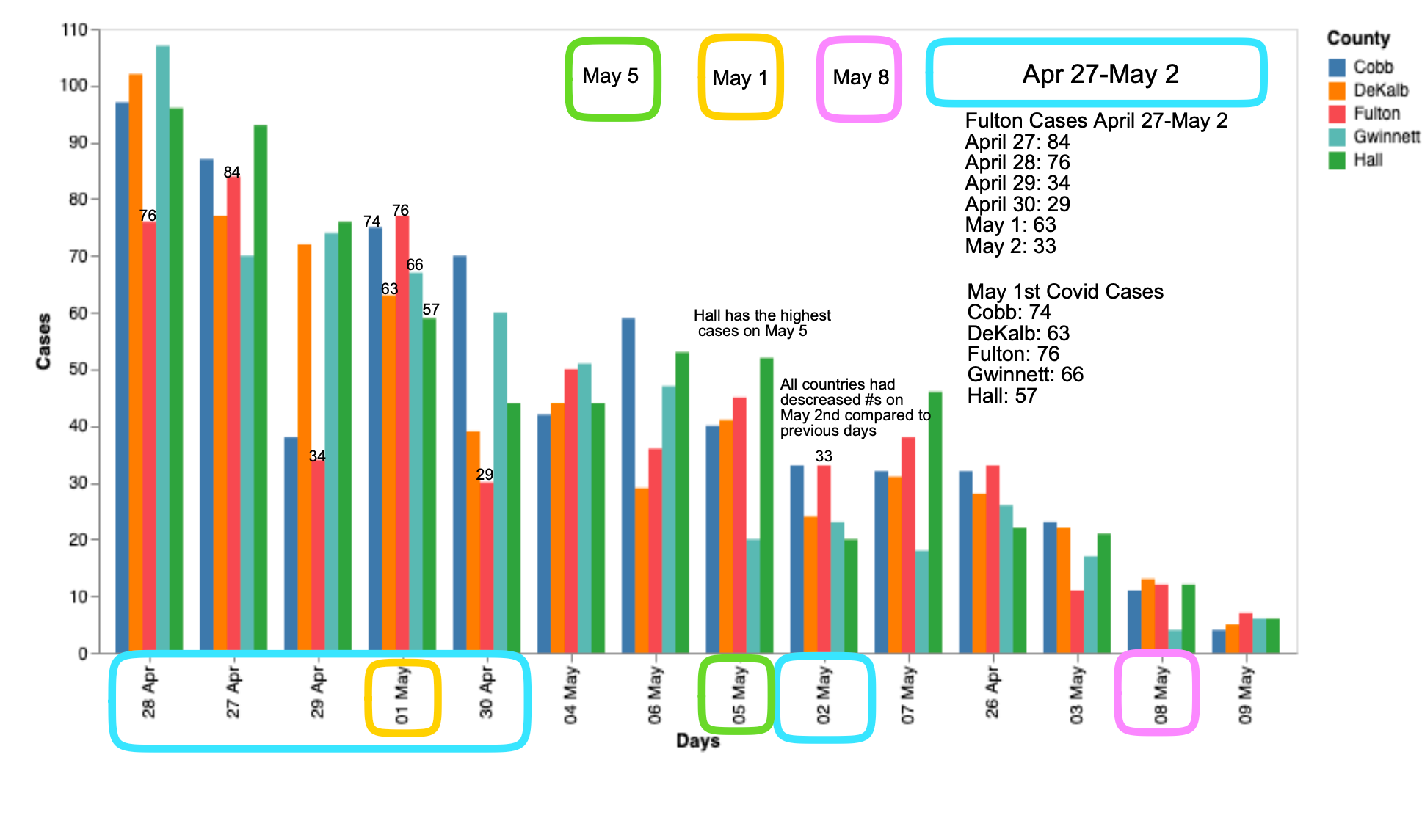
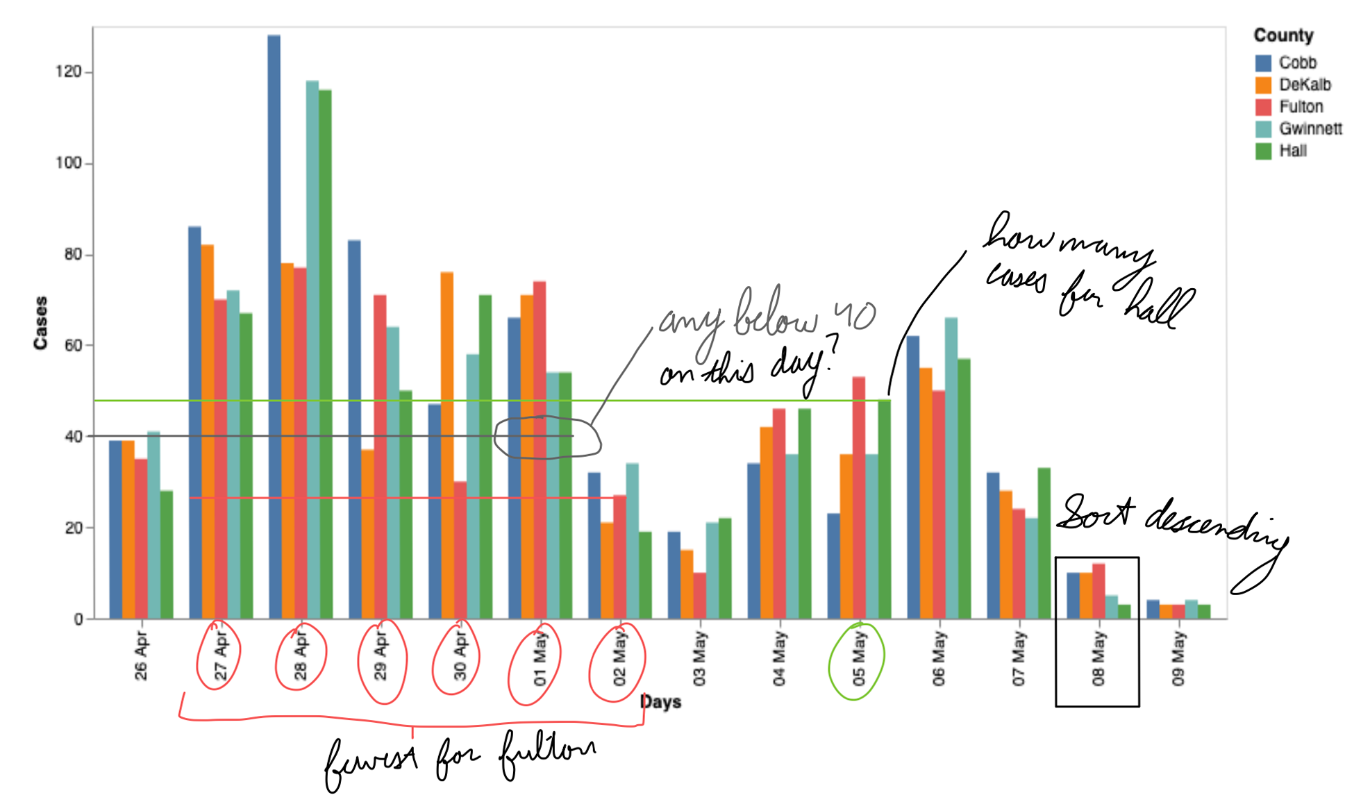
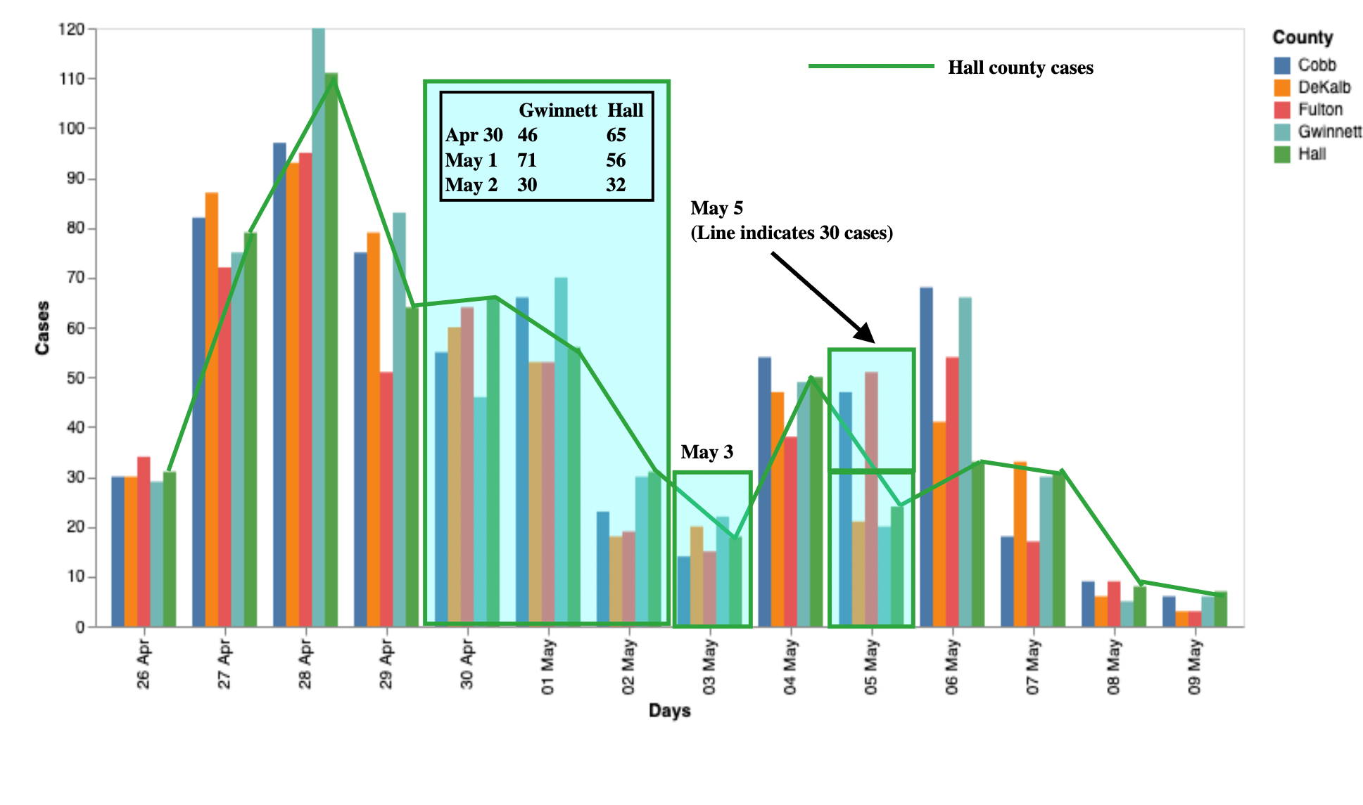
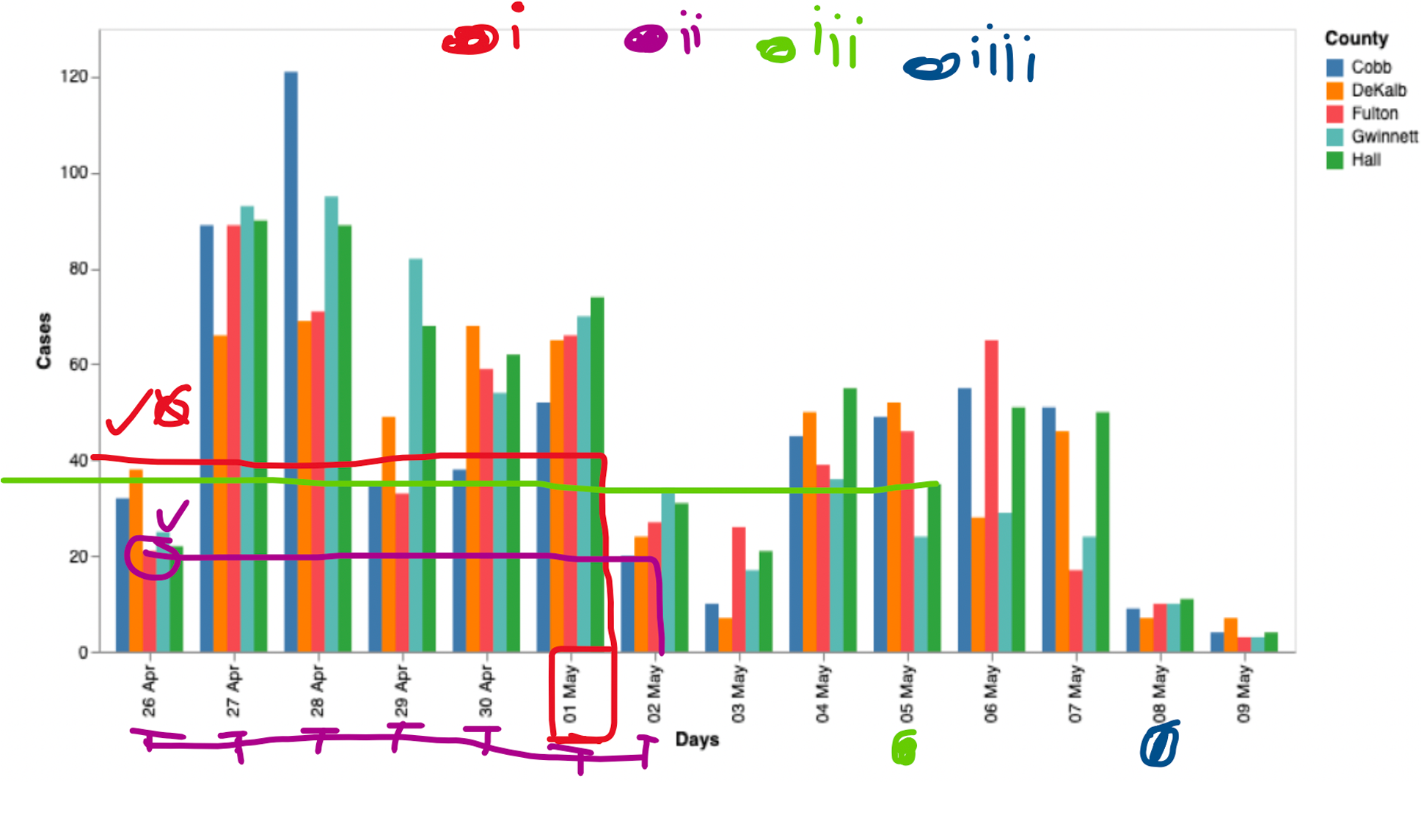
blackOliveGreen4pt

(a)

blackOliveGreen4pt

(b)

blackOliveGreen4pt

(c)

blackOliveGreen4pt

(d)

Figure 2: Four examples of annotations from Study 1. Despite being asked similar questions, we observed a variety of annotations coming from the students, which we coded into five types (enclosure, connector, text, mark, and color) that each support one or more low-level analytic tasks (retrieve value, filter, compute a derived value, find extremum, and sort). (a) One student used rectangles for filtering, text on bars for retrieving values and pointing out the extrema, and a legend for filtering important dates. (b) A second student annotated the chart with ellipses, rectangles, and lines for filtering, and text for filtering and as an identifier. (c) A third student used rectangles and highlights for filtering, text as an identifier, a trend line for finding extrema, and a legend for filtering. (d) A final example includes lines, circles, T-shaped, and circular marks.

Color

Color annotations are any property of color (generally, but not exclusively, hue) to answer questions about data, which is divided into second-level hierarchy categories, including highlights, category, questions, and values. The highlight-based annotations use different colors to highlight an area, bars, or group of bars (see LABEL:fig:example3) for a task. Color for values are annotations that aligns with text for value annotations (similar to a color map). The category-based color annotations highlight different categories (e.g., counties, dates/months, etc.) and are typically used in coordination with mark and enclosure annotations (i.e., as ensembles), e.g., the four different colors used for the date enclosures in LABEL:fig:example1. The question-based colors differentiate questions (e.g., Q1, Q2, etc.) used in coordination with mark-based annotations, e.g., the colored roman numerals in LABEL:fig:example5. From Table 1, color-based annotations were used heavily for all tasks, except sort, while highlights were only used for the filter task.

Other

The other category comprises symbols with special meaning. We found plus ($+$) used for denoting the addition operation of different values for the CDV task, delta ($\Delta$) for differentiating groups of bars, and pound ($\#$) used with an enclosure bracket for the CDV task.

4 Study 2: Real-World Annotation Practices

Study 1 provided a rich taxonomy of common annotation types within a limited context of grouped bar charts. The second study aimed to investigate how annotations were applied to diverse chart types in real-world settings and to determine whether the taxonomy developed in the first study exhibited generalizability across chart types employed in naturalistic contexts. To accomplish this, we obtained a large corpus of annotated images featuring commonly used chart types from Google Images and subjected them to a thematic coding procedure to ascertain patterns in the application of annotations.

4.1 Data Collected

We obtained 8768 images from Google Images using an image scrapping tool [32] (see Figure 3). We used different query keywords following the same pattern, “annotated {chart type}” (e.g., annotated pie chart, annotated scatterplot, annotated histogram, etc.). The queries included 15 chart types: line chart, bar chart, map, scatterplot, pie chart, bubble chart, donut chart, area chart, treemap, histogram, dashboard, graph (i.e., node-link diagrams), gantt chart, density map, and radar chart. Among the chart types collected, the distribution was not uniform, likely reflecting the popular use of those chart types. During our initial evaluations of the images, we removed 1244 duplicate images from the dataset. We then removed 4847 based upon additional exclusion criteria, including images with chart types that are not considered in the study, images with charts that are not clearly visible, images with charts without any annotations, and images with charts that do not represent any real data. This left a total of 2677 images in the dataset.

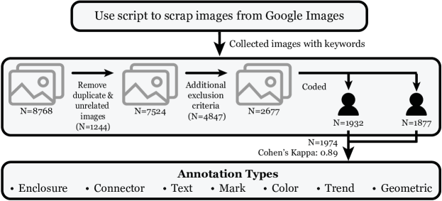
Figure 3: We scrapped annotated visualization images from Google Images using the search pattern “annotated {chart type}”, where the chart type included 15 commonly used charts (e.g., scatterplot). Two coders qualitatively coded the images into the seven annotation types shown.[DL: Use -> Used]

4.2 Data Coding

The dataset of images was coded using a thematic coding process, starting with the themes (i.e., the five categories of annotations) identified in the taxonomy found in Study 1. Two co-authors independently coded all 2677 images in multiple iterations with frequent meetings involving all authors to discuss and update the themes. Ultimately, the two coders identified 1932 and 1877 images, respectively, where the chart types relevant to the study were present, and the annotation type was not classified as “no annotation”, “undetermined” (i.e., ambiguous), or “other” (i.e., not a commonly practiced annotation type). When combining the results for both coders, a total of 1974 images were rated valid for the study. We evaluated the inter-rater reliability of our coding process using the Kappa statistic [31]. We compared the annotation types for the corresponding images between the raters and calculated the average Cohen’s Kappa coefficient of 0.886, which indicated a very high agreement between the raters. Thus, we utilized the annotations from the first coder for analysis. Results from both coders are on osf¹.

4.3 Taxonomy of Annotations

Upon analysis of the second study, we found that the taxonomy we established in our pilot study for bar chart annotations generalizes to other chart types. We identified frequent usage of the same high-level annotation types, including enclosures, connector, text, mark, and color (discussed in subsection 3.5). However, we also identified two new annotation types for our taxonomy, namely trend and geometric annotations. Figure 4 shows examples of all types of annotations.

Trend

For several chart types, we found a considerable number of annotations that indicate different trends in the data, such as trend lines representing a correlation relationship in scatterplots and changes in values over time or across different categories along a particular axis in bar charts. For example, we can see a line that shows Figure 4 shows that there is a positive correlation between test scores of students from different groups and time spent studying. In the classroom study, we observed the utilization of such trend lines, which were categorized as connectors at the time.

Geometric

For some chart types, we also observed frequent geometric operations, such as enlarging a specific area (e.g., a specific segment of the pie chart in LABEL:fig:teaser:f) or enlarging a portion of a chart (e.g., zooming in on regions of LABEL:fig:teaser:b or LABEL:fig:illustrative-scatterplot:g).

Appendix Table 1 shows the frequency distribution of different annotation types for different chart types. Text is the most commonly used annotation, appearing in approximately 44.5$\%$ of all annotations, followed by enclosures (16$\%$), trends (12.5$\%$), connectors (11.5$\%$), marks (7.7$\%$), color (7.6$\%$), and geometric (1.7$\%$) annotations.

5 Design Space for Annotations

We summarize the design space of common usages of annotations in visualization by looking at four different aspects of their usage. First, we discuss the role of the data source in constructing annotations. Second, we discuss the role of visual analytic tasks. Next, we identify patterns in which annotation types are frequently and infrequently used with which visualization types. Finally, we discuss the frequent use of certain combinations of annotations together, referred to as ensembles of annotations. Our design space is summarized in Figure 5.

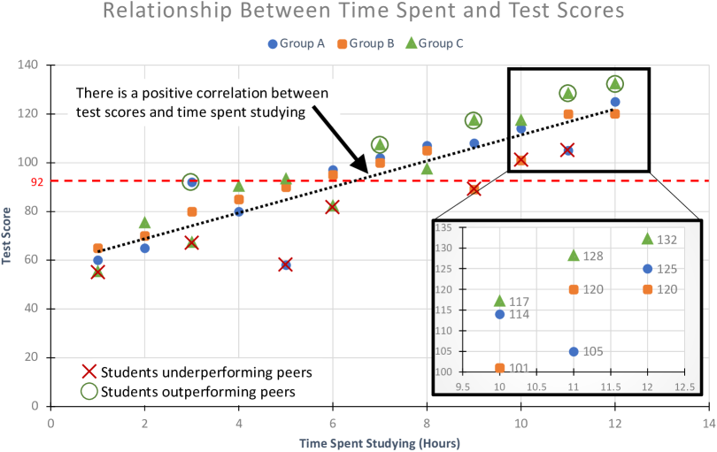
blackOliveGreen4pt

(a)

blackOliveGreen4pt

(b)

blackOliveGreen4pt

(c)

blackOliveGreen4pt

(d)

blackOliveGreen4pt

(e)

blackOliveGreen4pt

(f)

blackOliveGreen4pt

(g)

Figure 4: An illustrative example of annotations in a scatterplot showing (a) enclosure of a group of data, (b) a connector between text and a trend, (c) text describing the result, (d) mark and color that highlight certain data points, trend showing the (e) correlation and (f) average, and (g) a geometric annotation in the form of a zoom box.

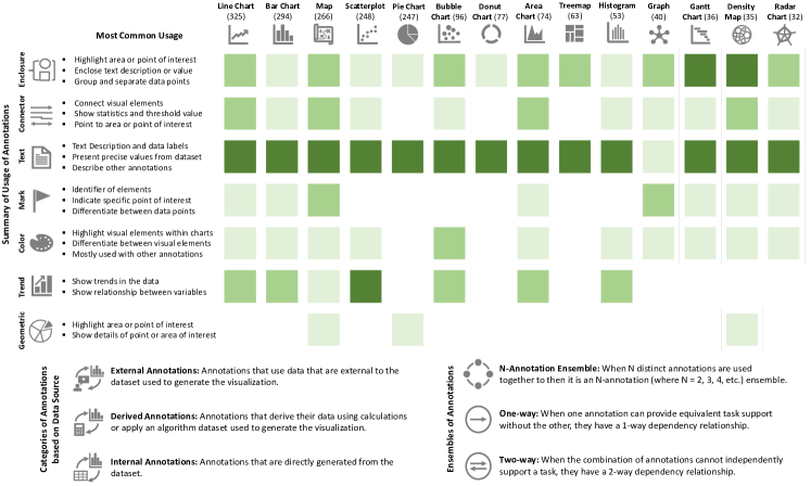
Figure 5: The Design Space of Common Practices in Annotations shows common uses of different annotations; color-coding based on the percentage of charts that used an annotation: 6-25% 26-50% 51+%; classification of annotation data sources; and types of annotation ensembles.

5.1 Data Source

One interesting observation made during Study 2 is that annotations used in charts can be classified based on the source of the data they were generated from. In particular, we identified three categories: external, derived, and internal data sources, which were included in the coding. This classification provides a useful framework for practitioners to understand where the data that generates annotations come from.

External Annotations

External annotations are those that do not come from the data that created the chart, but instead, they are created using an external data source (e.g., another data file, the internet, information coming from the visualization’s author, etc.). For example, in Figure 4, both the connector (LABEL:fig:illustrative-scatterplot:b) and the text (LABEL:fig:illustrative-scatterplot:c) are external annotations that collectively indicate the positive correlation between the Test Scores and Time Spent Studying variables because these annotations are external to the dataset and were manually generated to offer additional context to viewers. Similarly, the zoom box that provides contextual details for some data (LABEL:fig:illustrative-scatterplot:g) and the marks used to identify underperforming or outperforming students (LABEL:fig:illustrative-scatterplot:d) are also external annotations, as they were not generated from the original data, but were added manually to provide more information.

Derived Annotations

Derived annotations are calculated from the data represented by the chart, but do not directly represent values from the dataset. Statistical values and algorithms, such as clustering, are example sources for these types of annotations. In LABEL:fig:illustrative-scatterplot:e, the trend line depicting the correlation between the two variables is classified as a derived annotation since it was produced by applying an algorithm to the dataset that the chart conveys rather than directly representing any values from the dataset.

Internal Annotations

Internal annotations are taken directly from the dataset without requiring any calculations or input from sources outside the dataset. These annotations represent the exact values or text from the dataset and are generated automatically most of the time. An instance of internal annotations can be observed in LABEL:fig:illustrative-scatterplot:g, where the text labels associated with each data point represent exact values from the dataset, hence being generated directly from it. Similarly, the text labels in LABEL:fig:teaser:a for the bars in the bar chart and in LABEL:fig:teaser:f for the pies in the pie chart represent exact values from the dataset, making them internal annotations.

5.1.1 Common Patterns for Data Sources

Table 2 shows the frequency distribution of three different categories of annotations for different annotation types.

External annotations have the highest frequency in five annotation types, i.e., enclosure, connector, text, mark, and geometric, suggesting that external annotations are the most commonly used across different chart types. There might be several reasons why external annotations are common in practice. Firstly, they offer a high degree of flexibility, allowing users to add annotations that are important for conveying the message or meaning of the visualization, even if they are not directly related to the data. For example, a user might add a text annotation to provide context or explain a trend in the data. This flexibility is crucial because it enables users to create more engaging and compelling visualizations to communicate their intended message. Secondly, external annotations allow personalizing of the visualizations to help convey a specific message more effectively. This is particularly important in domains where the interpretation of data is subjective or where there are multiple possible explanations for a trend or pattern.

Table 2: Frequency of different annotation categories based on their data source. Box colors indicate frequency: 5-50 50-300 300+.

Our analysis indicates that derived annotations have a generally low frequency. The most frequently used derived annotations were the trend annotations that denoted, e.g., the correlation relationship between two variables. An example is shown in LABEL:fig:illustrative-scatterplot:e. Moreover, various other types of derived annotations were utilized to represent statistical information. For instance, vertical lines were commonly used in histograms to depict the mean of the distribution. The lower frequency of derived annotations can be attributed to their limited flexibility compared to external annotations and the greater difficulty in generating them compared to internal annotations.

Internal annotations are widely used, with text annotations being the most commonly occurring type. This high frequency indicates that text is crucial for effectively communicating information directly from the dataset. Enclosure and connector annotations were also used relatively frequently, often in conjunction with text annotations. Internal annotations are frequently used for several reasons. First, they offer a high level of precision and accuracy since they represent exact values generated directly from the dataset. Second, they are less prone to human error and can be more precise than manual annotations. Finally, they tend to be consistent across different parts of the visualization, which makes it easier for viewers to compare and interpret the data, potentially reducing bias in the annotations.

5.2 Task Support of Annotations

The kinds of tasks annotations support is crucial to understanding their best practice uses. In Study 1, we observed non-uniform support for various low-level tasks by different annotation types (see Table 1).

For the Retrieve Value (RV) task, we saw broad support from individual annotation types. In particular, connector and color seemed to be used frequently to identify (i.e., using color) and draw attention to the data (i.e., using the connector). Given the many options available, RV seems to be one of the easier tasks to annotate. Find Extremum (FE) annotation usage closely mirrors that of RV, given the FE is often just a special case of RV. Text and connector annotations were the ones used most frequently. Similar to RV, the Filter task saw universal support from the various annotation types, making it one of the easier tasks to annotate. As one of the main goals of annotation is highlighting particular data (i.e., filtering), it makes sense that the types of annotations participants chose would generally be useful for filtering. Participants used text, color, and enclosure most frequently for the Compute Derived Value (CDV) task. These annotations indicate that participants often had to filter the data according to some criteria, then compute something (e.g., add, average, etc.) on the filtered data. To denote all these steps, the participant used enclosures to isolate the data, color to highlight, and text to explain, indicating the compound nature of the CDV task. Finally, the Sort task appeared challenging to annotate. Most often, participants relied upon text, sometimes with connectors, to describe the part of the charts that needed to be sorted.

5.2.1 Common Patterns for Tasks

Many of the task annotations patterns identified in Study 1 were also present in Study 2. However, an explicit mapping of tasks to annotations was unavailable due to the lack of information about the annotation designer’s intent. Nevertheless, our analysis revealed consistent patterns that allowed us to infer the tasks that were likely being performed.

The most frequent type of annotation used across various chart types was the display of exact data labels of individual data points from the dataset (i.e., retrieve value and find extremum tasks). An example of this can be seen in LABEL:fig:teaser:f, where the data labels for each pie in the pie chart are explicitly provided, and in LABEL:fig:illustrative-scatterplot:c, where the corresponding values of certain data points on the line are given, enabling viewers to retrieve the values quickly. Also, as depicted in LABEL:fig:illustrative-scatterplot:f, we observed a significant use of connectors (e.g., lines) to emphasize specific values on particular axes, thus aiding viewers in retrieving them more easily. These annotations were particularly prominent in chart types that feature axes, including scatterplots, line charts, bar charts, and histograms.

We also observed the predominant use of different enclosures for filtering a specific data point, multiple data points, or a specific region of interest. Sometimes these enclosures were accompanied by a zoom box to emphasize a particular chart region, further supporting filtering. For instance, in LABEL:fig:illustrative-scatterplot:a and LABEL:fig:teaser:b, rectangle enclosures are combined with a zoom box to filter the data. These enclosures were frequently accompanied by other annotations, e.g., connectors and texts.

We also found frequent support for computing derived values. The obvious example of this task comes in the form of trend annotations, such as the correlation in LABEL:fig:illustrative-scatterplot:e. On occasion, we found annotations that assisted in deriving other numbers from a chart, although they were infrequent. An example, shown in LABEL:fig:teaser:a, has the connectors aiding in comparing values and deriving the differences between the bars.

Finally, we did not see any consistent use of annotations to support sorting, possibly indicating that such a task is either not important or not easily supported by annotations.

This list of tasks is not exhaustive and requires further analysis. Nevertheless, our observations of common task support for various annotation types are shown in Figure 5 under Most Common Usage.

5.3 Common Patterns of Annotation Types

We examine how different annotation types are used in different chart types so that practitioners and designers can gain insights into best practices and common approaches to visualization design.

Usage of Text Annotations

Throughout our analysis, we have observed a prevalence of the use of text annotations in all chart types. Specifically, we observed that a total of 1469 charts out of 1974 charts used text annotations, which confirms that people like text annotations over other annotation types in practice. Text annotations were utilized in diverse ways across different chart types, serving a range of purposes such as describing chart elements, providing additional context about the data, indicating direct values from the dataset, specifying data point labels, explaining other graphical annotations, and more. The widespread use of text annotations across all chart types can be attributed to several factors. The foremost among them is their flexibility, which enables conveying a diverse range of information with varying levels of detail. Text annotations can be employed to provide simple labels, detailed descriptions, brief summaries, or in-depth explanations, depending on the purpose of the visualization and the audience’s needs. As shown in LABEL:fig:illustrative-scatterplot:g, the exact values for some data points are depicted within the chart. Moreover, text annotations can offer additional contexts, such as the data source, the units of measurement, relevant background, etc. Furthermore, we noticed that people commonly used text annotations alongside other forms of annotation to offer additional context or clarification to the visualization. For instance, in LABEL:fig:illustrative-scatterplot:c, despite the presence of a correlation line to denote a positive correlation between the two variables, a text description is used to explain the relationship explicitly.

Usage of Enclosures

Enclosure annotations were frequently utilized in all chart types, similar to text annotations. These annotations were primarily used to group related information and make it easier for viewers to interpret the data. For example, in LABEL:fig:illustrative-scatterplot:a, a rectangle has been used to group a set of data points. Enclosures can also act as a container for text annotations and separate the enclosed data from other elements within the chart. Enclosures can also be used in various other ways, such as highlighting a particular bar in a bar chart, a specific section of a line chart, a particular area of interest in maps, or particular nodes in a graph.

Usage of Connectors

We observed connectors such as arrows and lines in most of the chart types. However, they were primarily used in conjunction with other annotation types, as discussed in subsection 5.4. Their purpose is to establish a visual connection between the point or area of interest and the text description or enclosure containing text description, making it easier for viewers to understand which annotation corresponds to which area of interest as shown in LABEL:fig:illustrative-scatterplot:b. Furthermore, lines can be useful along a specific axis showing a threshold, statistical, or benchmark value in some chart types. They can also be used to compare different data points or areas of interest within a chart, such as connecting two bars in a bar chart to show the difference between them as shown in LABEL:fig:teaser:a. Also, connectors can be customized with color, thickness, and other style parameters, allowing for greater flexibility in terms of their usage and visual impact.

Usage of Marks

Marks were mainly used as identifiers or visual indicators in different chart types. We noticed the most prominent use of marks in maps. In maps, marks were used to pin different points of interest or regions. Also, marks were used in line charts to indicate specific points of interest along the plotted line, as depicted in LABEL:fig:teaser:e. Similarly, marks were applied in bar charts to identify the bar(s) of interest or to highlight specific point(s) on any of the chart axes. In scatterplots, marks were employed to distinguish particular data points from others or to highlight single or multiple points of interest. For example, in LABEL:fig:illustrative-scatterplot:d, marks are employed with color to identify and differentiate the data points representing students who are underperforming and outperforming their peers.

Usage of Color

Color is a highly effective means of visually distinguishing between different categories or data points and drawing attention to specific elements or regions of a visualization. Color was always combined with other annotations. Color annotations are utilized in various chart types, including line charts, bar charts, maps, scatterplots, bubble charts, and area charts. The primary function of color is to highlight a specific data point or set of data points, as exemplified in LABEL:fig:illustrative-scatterplot:d, where color has been used with marks to differentiate some data points from others. Here, data points representing underperforming students are denoted by red-colored cross marks, while green-colored ellipses indicate data points representing outperforming students. Additionally, color is employed to highlight specific regions of a chart, such as areas of interest in maps, and to differentiate between categories or groups in a chart, such as using colors to differentiate between the clusters. It is important to note that encodings inherent to the charts are not considered annotations, such as color encoding for different categories in a scatterplot, e.g., in Figure 4, or color encoding for different bars indicating different categories in a grouped bar chart, with the use of legends.

Usage of Trends

Trend annotations were frequently used in many chart types. In bar charts, histograms, line charts, and area charts, trend lines are often utilized to depict changes in values along a particular axis, whether in direction (e.g., upward or downward) or magnitude (e.g., rapid or slower). Conversely, in scatterplots (see LABEL:fig:illustrative-scatterplot:e) and bubble charts, trend lines are primarily used to show the correlation relationship (e.g., positive or negative correlation) between variables. Additionally, they differentiate between clusters in scatterplots, allowing for more precise data interpretation (see LABEL:fig:teaser:d). Trend annotations are not commonly used in visualizations such as pie charts, donut charts, radar charts, treemaps, and density maps because these visualizations do not have an axis to indicate a trend. For instance, pie charts represent proportions, and the slices do not have any inherent order. Similarly, treemap data do not have an explicit order.

Usage of Geometric Annotations

Geometric annotations were observed to be more prevalent in certain chart types, namely pie charts, maps, and donut charts, to draw attention to a specific section of the chart. In pie and donut charts, where each wedge or slice represents a portion of a whole, it may be necessary to emphasize a particular section if it contains crucial information or is of significant interest to the viewer (see LABEL:fig:teaser:f). In  LABEL:fig:illustrative-scatterplot:g, the scatterplot has been zoomed in on a specific portion to provide additional context to the viewers. Similarly, in maps, zooming in on a specific area can help provide greater detail and clarity, particularly if the information displayed is complex or detailed. However, the suitability of geometric annotations relies on the chart type, the data type, and the message the visualization intends to convey. For example, in a bar chart, zooming in on a particular bar or section may not be necessary or practical. Similarly, in a line chart, zooming in on a specific section may cause the viewer to lose sight of the overall trend in the data.

5.4 Ensemble Annotations

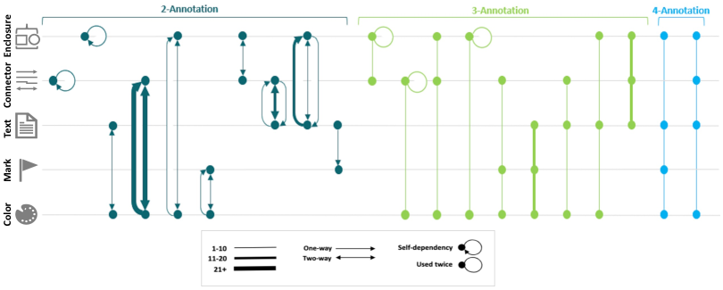
Figure 6: Visualization showing the configuration and frequency of annotation ensembles from Study 1. Each row denotes an annotation type, and each column denotes a particular annotation ensemble. The points indicate which individual ensemble was used, while the lines and arrows indicate their relationship. The width of the lines denotes the frequency with which the ensembles were observed.

In both studies, we observed that in cases where a single annotation type was insufficient to convey the intended information, people resorted to using a combination of multiple annotations. Figure 7 contains many examples of ensembles from Study 1, including connector–text used to identify particular values, enclosure–text denoting data to sort, and enclosure–color–text for filtering data. This happened for several reasons. For one, when the data of interest is too complicated to describe with individual annotations, multiple annotations were used. Secondly, when visual elements would interfere with the annotation (e.g., identifying a single bar), multiple annotations, usually including connectors, would be used.

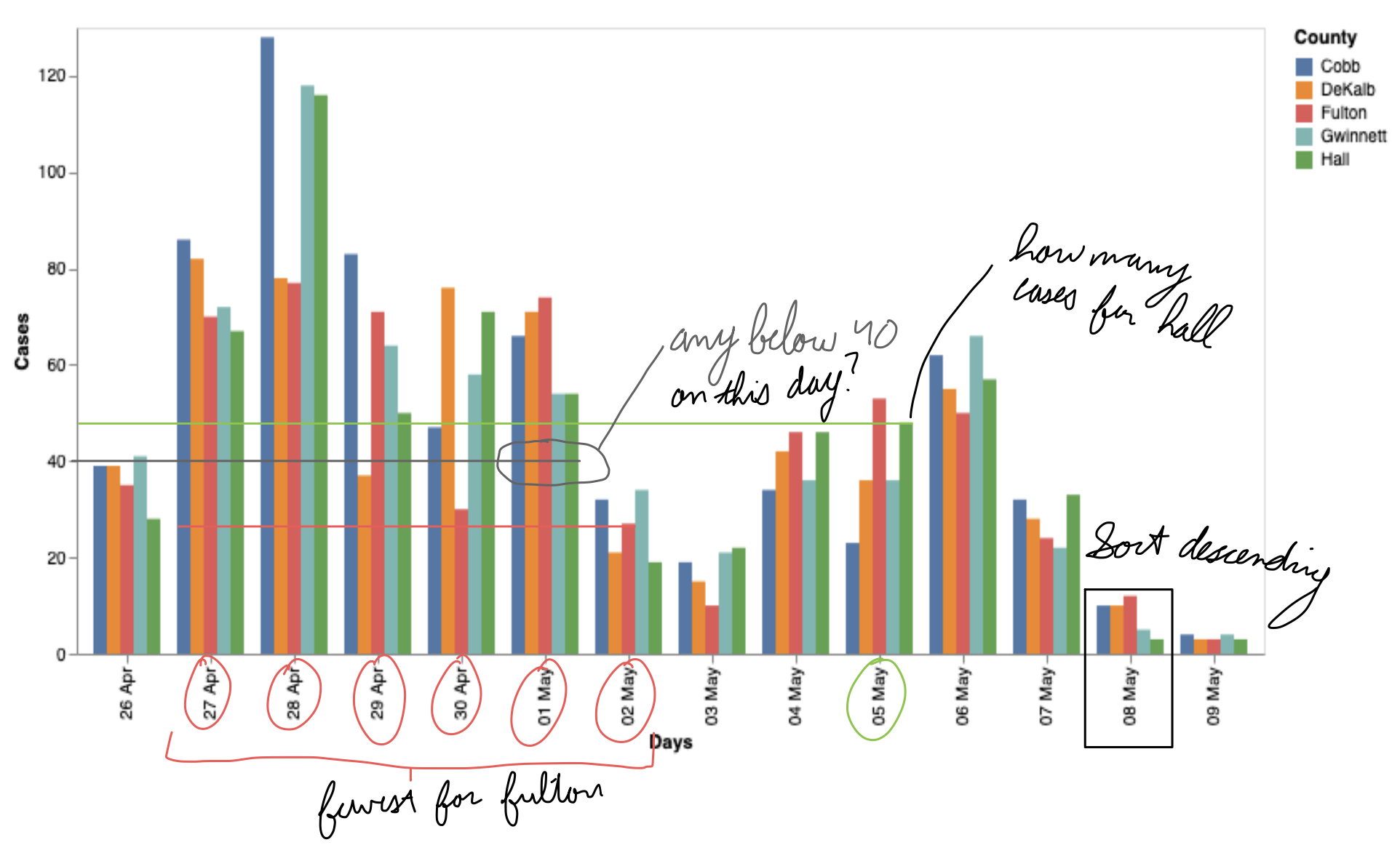
Figure 7: An example of ensembles where ellipse–bracket–text (i.e., enclosure–enclosure–text) is to filter dates from April 27 to May 2, ellipse–line–text (i.e., enclosure–connector–text) is to filter counties with more than 40 covid cases on May 1, and line–text–color (i.e., connector–text–color) is to find the total number of covid cases for Hall on May 5.

N-Annotation Ensembles

The resulting ensembles are divided into categories based on the number of individual annotations used in the ensembles, which we identify as 2-annotation, 3-annotation, and 4-annotation ensembles and generally refer to as N-annotations. Figure 6 summarizes the ensembles identified during Study 1, based upon the data in Appendix Table 3. We do not consider the summary a complete set of annotation ensembles. Instead, it is a representative set of possibilities. 2-Annotation Ensembles: Overall, in Study 1, 2-ensembles were very common, with connector–color being the most frequently used, in addition to text–connector and text–enclosure. 3-Annotation Ensembles: Overall, the most frequently used 3-annotation ensembles were enclosure–connector–text and text–mark–color. For example, in Figure 7, enclosure–connector–text is used to denote the task that filters counties with fewer than 40 covid cases on May 1. 4-Annotation Ensembles: We observed a small number of 4-annotations in Study 1 that were of the type enclosure–connector–text–color or enclosure–text–mark–color. One important observation is that when four or more different annotation types are combined, the annotations are often redundant or unnecessary. In other words, it is possible that a 2- or 3-annotation could have been used instead.

We further classified N-annotation ensembles into categories based on the dependency relationship between the individual annotations.

One-way

One-way annotation occurs when one of the annotations does not require the other to convey its information. Instead, the additional annotation complements the independent one to accomplish the task. For example, in Figure 7, the red color provides no additional value besides emphasizing the other annotation.

Two-way

Two-way annotation ensembles occur when neither of the annotations can stand independently without the help of the other (i.e., they are mutually dependent on each other). For example, in Figure 7, the connector–text annotations are mutually required to understand the purpose of both the text and the connector.

5.4.1 Common Patterns for Ensemble Usage

Our investigation in Study 2 has uncovered significant use of ensemble annotations. While a definitive enumeration of the number of ensemble annotations was not conducted due to the lack of explicit information regarding the corresponding annotation designer intention, we observed consistent patterns of ensemble usage in our analysis. The most frequently used ensembles across different chart types were enclosure–connector–text, connector–text, enclosure–text, and mark–color, which were also prevalent in Study 1. In these ensembles, enclosures were primarily utilized to highlight or separate text, while connectors were used to establish a relationship between the corresponding data point within the chart and the text or the enclosure with text. For instance, in LABEL:fig:illustrative-scatterplot:b, a connector (i.e., the arrow) was used to link the correlation and the text explaining the relationship. Color was frequently used with marks, text, connectors, and enclosures to differentiate, identify, or highlight certain categories in different charts. For example, in LABEL:fig:illustrative-scatterplot:d, color and marks were used to identify the data points representing the underperforming and outperforming students.

6 Discussion & Conclusions

6.1 Using the Design Space

One of the key insights we are interested in remains gaining a better understanding of the design space for annotations. We frequently use annotations, knowingly or unknowingly, in our daily lives. For example, in a presentation, annotations enable a presenter to draw the attention of the viewers to an important point of focus [27]. So, what are the uses of the design space in Figure 5?

A structured way to think about constructing and critiquing annotations

By combining common practices for data, task, and encoding, our design space enables an individual authoring annotations to decide, in a systematic way, what annotations to use. The design space also provides a structured method for critiquing others’ work by identifying and categorizing the key elements used in their annotations.

Opening up the space of annotations

Despite annotations being a tool used nearly every day, the space of possible annotations encodings available was not initially obvious to us. The design space provides a comprehensive list of annotation types available for visualizations. Importantly, within this design space, whether intentional or not, the annotations we observed participants using seemed closely linked to the idea of encoding semantics [49].

Avoiding uncommon practices (or making sure to use common practices)

Figure 5 differentiates which annotation types are commonly used in practice with particular visualization types. By observing frequently and infrequently used combinations, annotation authors can avoid creative combinations that might confuse their audience.

6.2 Ecological Validity

In Study 1, we asked visualization students to annotate bar charts based on a set of high-level questions. These individuals represent neither experts nor the general population—they were sufficiently well-versed in visualizations to know how to use them effectively but not so experienced as to have a set of standard practices to draw upon for annotation. Therefore, in isolation, it is difficult to say how well the conclusions on their practices extrapolate. Furthermore, the use of bar charts only was limiting. Finally, their tasks were provided to them in an open-ended format that represented the type of task someone might perform when annotating a chart, providing a diverse picture of the potential design space available for annotations. Given these factors, the study has high ecological validity but within a narrow context.

In Study 2, we collected images containing 15 different chart types and coded them using the themes from Study 1. We did not have specific information about the annotation designer’s intent, what tools they used, or their level of expertise in visualization. Despite these limitations, when we analyzed the data, we found similar annotations being used as in Study 1, which suggests the broad applicability of our initial taxonomy beyond the specific context of that study. Given that the data was collected from a diverse set of real-world sources, the study has high ecological validity in broad contexts.

6.3 Limitations

Our proposed taxonomy and design space are based on a qualitative study of the annotations applied by visualization students to bar charts and the annotations utilized by individuals in real-world settings for various chart types. However, we have not conducted an evaluation of the effectiveness of any annotation type in any chart type. Consequently, we are unable to make definitive claims regarding the efficiency of particular annotations for specific chart types. Nonetheless, we plan a future investigation to examine their efficacy in a variety of scenarios.

It is important to note that the scope of our research was limited to static visualizations in both studies. As a result, we did not explore the use of dynamic or interactive visualizations with dynamic and interactive annotations. However, we recognize the significance of these modalities in modern data visualization and plan to investigate the utilization of annotations in these contexts in the future.

6.4 Conclusions

Annotations support the visual exploration of data and provide a salient visual aid to users. They can be used to help generate hypotheses, communicate information, assist in sense-making, and analyze charts collaboratively. Understanding the use of annotations in visualizations, can provide design guidelines for collaborative user-analytic tasks and for knowledge transfer. Our findings provide a comprehensive taxonomy of annotation types that can be used across different chart types. This standardized framework for annotating visualizations offers valuable insights into the design space for annotations, allowing practitioners to explore the space of possible annotation types. By proposing a design space that includes common practices for combinations of annotations and visualization pairings, data sources, and ensembles, we hope to encourage the development of more effective and efficient visualizations that can support better user engagement, understanding, and decision-making across a variety of domains.

Notes

1. 1 https://osf.io/dfhn6/?view_only=0ce9b009c8764c75bded7f88cd74b949
2. 2 In Study 1, students had previously been exposed to encoding semantics several weeks prior, but we suspect that the relationship was unintentional.

- [1] R. Amar, J. Eagan, and J. Stasko. Low-level components of analytic activity in information visualization. In IEEE Symposium on Information Visualization (InfoVis), pp. 111–117, 2005. doi: 10 . 1109/INFVIS . 2005 . 1532136
- [2] M. Borkin, A. A. Vo, Z. Bylinskii, P. Isola, S. Sunkavalli, A. Oliva, and H. Pfister. What makes a visualization memorable? IEEE Transactions on Visualization and Computer Graphics, 19(12):2306–2315, 2013. doi: 10 . 1109/TVCG . 2013 . 234
- [3] S. Breslav, R. Goldstein, A. Khan, and K. Hornbæk. Exploratory sequential data analysis for multi-agent occupancy simulation results. In Symposium on Simulation for Architecture & Urban Design, pp. 59–66, 2015. doi: 10 . 5555/2873021 . 2873030
- [4] A. Cedilnik and P. Rheingans. Procedural annotation of uncertain information. In IEEE Visualization, pp. 77–84, 2000. doi: 10 . 1109/VISUAL . 2000 . 885679
- [5] Y. Chen, J. Alsakran, S. Barlowe, J. Yang, and Y. Zhao. Supporting effective common ground construction in asynchronous collaborative visual analytics. In IEEE Symposium on Visual Analytics in Science and Technology (VAST), pp. 101–110, 2011. doi: 10 . 1109/VAST . 2011 . 6102447
- [6] Y. Chen, S. Barlowe, and J. Yang. Click2annotate: Automated insight externalization with rich semantics. In IEEE Symposium on Visual Analytics in Science and Technology (VAST), pp. 155–162, 2010. doi: 10 . 1109/VAST . 2010 . 5652885
- [7] Y. Chen, J. Yang, S. Barlowe, and D. Jeong. Touch2annotate: Generating better annotations with less human effort on multi-touch interfaces. In ACM SIGCHI Conference on Human Factors in Computing Systems (Extended Abstracts), pp. 3703–3708, 2010. doi: 10 . 1145/1753846 . 1754042
- [8] G. Chin Jr, O. A. Kuchar, and K. E. Wolf. Exploring the analytical processes of intelligence analysts. In ACM SIGCHI Conference on Human Factors in Computing Systems, pp. 11–20, 2009. doi: 10 . 1145/1518701 . 1518704
- [9] R. Chun. Giving guidance to graphs: Evaluating annotations of data visualizations for the news. Visual Communication Quarterly, 27(2):84–97, 2020. doi: 10 . 1080/15551393 . 2020 . 1749842
- [10] S. Collins. Georgia’s covid-19 cases aren’t declining as quickly as initial data suggested they were. Vox, 2020.
- [11] S. Ellis and D. P. Groth. A collaborative annotation system for data visualization. In Advanced Visual Interfaces, pp. 411–414, 2004. doi: 10 . 1145/989863 . 989938
- [12] A. Fan, Y. Ma, M. Mancenido, and R. Maciejewski. Annotating line charts for addressing deception. In ACM SIGCHI Conference on Human Factors in Computing Systems, 2022. doi: 10 . 1145/3491102 . 3502138
- [13] J. Heer and B. Shneiderman. Interactive dynamics for visual analysis. Communications of the ACM, 55(4):45–54, 2012. doi: 10 . 1145/2133806 . 2133821
- [14] J. Heer, F. Viégas, and M. Wattenberg. Voyagers and voyeurs: supporting asynchronous collaborative information visualization. In ACM SIGCHI Conference on Human Factors in Computing Systems, pp. 1029–1038, 2007. doi: 10 . 1145/1240624 . 1240781
- [15] A. Hopkins, M. Correll, and A. Satyanarayan. Visualint: Sketchy in situ annotations of chart construction errors. Computer Graphics Forum, 39(3):219–228, 2020. doi: 10 . 1111/cgf . 13975
- [16] J. Hullman and N. Diakopoulos. Visualization rhetoric: Framing effects in narrative visualization. IEEE Transactions on Visualization and Computer Graphics, 17(12):2231–2240, 2011. doi: 10 . 1109/TVCG . 2011 . 255
- [17] J. Hullman, N. Diakopoulos, and E. Adar. Contextifier: automatic generation of annotated stock visualizations. In ACM SIGCHI Conference on Human Factors in Computing Systems, pp. 2707–2716, 2013. doi: 10 . 1145/2470654 . 2481374
- [18] T. Isenberg, P. Neumann, S. Carpendale, S. Nix, and S. Greenberg. Interactive annotations on large, high-resolution information displays. In Conference Compendium of IEEE VIS, IEEE InfoVis, and IEEE VAST, pp. 124–125, 2006.
- [19] N. Kadivar, V. Chen, D. Dunsmuir, E. Lee, C. Qian, J. Dill, C. Shaw, and R. Woodbury. Capturing and supporting the analysis process. In IEEE Symposium on Visual Analytics in Science and Technology (VAST), pp. 131–138, 2009. doi: 10 . 1109/VAST . 2009 . 5333020
- [20] Y.-a. Kang, C. Gorg, and J. Stasko. Evaluating visual analytics systems for investigative analysis: Deriving design principles from a case study. In IEEE Symposium on Visual Analytics in Science and Technology (VAST), pp. 139–146, 2009. doi: 10 . 1109/VAST . 2009 . 5333878
- [21] Y.-a. Kang and J. Stasko. Characterizing the intelligence analysis process through a longitudinal field study: Implications for visual analytics. Information Visualization, 13(2):134–158, 2014. doi: 10 . 1177/1473871612468877
- [22] H.-K. Kong, Z. Liu, and K. Karahalios. Internal and external visual cue preferences for visualizations in presentations. Computer Graphics Forum, 36(3):515–525, 2017. doi: 10 . 1111/cgf . 13207
- [23] N. Kong and M. Agrawala. Perceptual interpretation of ink annotations on line charts. In ACM Symposium on User Interface Software and Technology (UIST), pp. 233–236, 2009. doi: 10 . 1145/1622176 . 1622219
- [24] N. Kong and M. Agrawala. Graphical overlays: Using layered elements to aid chart reading. IEEE Transactions on Visualization and Computer Graphics, 18(12):2631–2638, 2012. doi: 10 . 1109/TVCG . 2012 . 229
- [25] R. Kosara and J. Mackinlay. Storytelling: The next step for visualization. Computer, 46(5):44–50, 2013. doi: 10 . 1109/MC . 2013 . 36
- [26] S. Latif, D. Liu, and F. Beck. Exploring interactive linking between text and visualization. In EuroVis (Short Papers), pp. 91–94, 2018.
- [27] B. Lee, R. Kazi, and G. Smith. Sketchstory: Telling more engaging stories with data through freeform sketching. IEEE Transactions on Visualization and Computer Graphics, 19(12):2416–2425, 2013. doi: 10 . 1109/TVCG . 2013 . 191
- [28] B. Lee, N. H. Riche, P. Isenberg, and S. Carpendale. More than telling a story: Transforming data into visually shared stories. IEEE Computer Graphics and Applications, 35(5):84–90, 2015. doi: 10 . 1109/MCG . 2015 . 99
- [29] N. Mahyar, A. Sarvghad, and M. Tory. Note-taking in co-located collaborative visual analytics: Analysis of an observational study. Information Visualization, 11(3):190–204, 2012. doi: 10 . 1177/1473871611433713
- [30] C. Marshall and A. B. Brush. Exploring the relationship between personal and public annotations. In ACM/IEEE-CS Joint Conference on Digital libraries, pp. 349–357, 2004. doi: 10 . 1145/996350 . 996432
- [31] M. L. McHugh. Interrater reliability: the kappa statistic. Biochemia Medica, 22(3):276–282, 2012. doi: 10 . 11613/BM . 2012 . 031
- [32] Ohyicong. Ohyicong/google-image-scraper: A library to scrap google images.
- [33] A. Ottley, A. Kaszowska, R. J. Crouser, and E. M. Peck. The curious case of combining text and visualization. EuroVis (Short Papers), 2019.
- [34] M. D. Rahman, G. J. Quadri, and P. Rosen. A qualitative evaluation and taxonomy of student annotations on bar charts. In VisComm Workshop at IEEE VIS, 2022.
- [35] M. Raschke, S. Strohmaier, T. Blascheck, and T. Ertl. Annotation of graphical elements in visualizations for an efficient analysis of visual tasks. In ACM SIGCHI Conference on Human Factors in Computing Systems (Extended Abstracts), pp. 1387–1398, 2014. doi: 10 . 1145/2559206 . 2581305
- [36] D. Ren, M. Brehmer, B. Lee, T. Höllerer, and E. K. Choe. Chartaccent: Annotation for data-driven storytelling. In IEEE Pacific Visualization Symposium (PacificVis), pp. 230–239, 2017. doi: 10 . 1109/PACIFICVIS . 2017 . 8031599
- [37] P. M. Sanderson and C. Fisher. Exploratory sequential data analysis: Foundations. Human–Computer Interaction, 9(3-4):251–317, 1994. doi: 10 . 1207/s15327051hci0903&4_2
- [38] A. Satyanarayan and J. Heer. Authoring narrative visualizations with ellipsis. Computer Graphics Forum, 33(3):361–370, 2014.
- [39] A. Satyanarayan, D. Moritz, K. Wongsuphasawat, and J. Heer. Vega-lite: A grammar of interactive graphics. IEEE Transactions on Visualization and Computer Graphics, 23(1):341–350, 2016. doi: 10 . 1109/TVCG . 2016 . 2599030
- [40] E. Segel and J. Heer. Narrative visualization: Telling stories with data. IEEE Transactions on Visualization and Computer Graphics, 16(6):1139–1148, 2010. doi: 10 . 1109/TVCG . 2010 . 179
- [41] R. Sevastjanova, M. El-Assady, A. J. Bradley, C. Collins, M. Butt, and D. Keim. Visinreport: Complementing visual discourse analytics through personalized insight reports. IEEE Transactions on Visualization and Computer Graphics, p. preprint, 2021. doi: 10 . 1109/TVCG . 2021 . 3104026
- [42] Y. B. Shrinivasan, D. Gotzy, and J. Lu. Connecting the dots in visual analysis. In 2009 IEEE symposium on visual analytics science and technology, pp. 123–130. IEEE, 2009.
- [43] Simon-Gd. Simon-gd/ubertagger: Exploratory analysis and annotation of sequntial data, 2015.
- [44] J. Stasko, C. Görg, and Z. Liu. Jigsaw: supporting investigative analysis through interactive visualization. Information Visualization, 7(2):118–132, 2008. doi: 10 . 1057/palgrave . ivs . 9500180
- [45] C. Stokes, V. Setlur, B. Cogley, A. Satyanarayan, and M. A. Hearst. Striking a balance: Reader takeaways and preferences when integrating text and charts. IEEE Transactions on Visualization and Computer Graphics, 29(1):1233–1243, 2022. doi: 10 . 1109/TVCG . 2022 . 3209383
- [46] E. R. Tufte. The visual display of quantitative information. Journal for Healthcare Quality (JHQ), 7(3):15, 1985. doi: 10 . 1097/01445442-198507000-00012
- [47] F. B. Viegas, M. Wattenberg, F. Van Ham, J. Kriss, and M. McKeon. Manyeyes: a site for visualization at internet scale. IEEE Transactions on Visualization and Computer Graphics, 13(6):1121–1128, 2007. doi: 10 . 1109/TVCG . 2007 . 70577
- [48] K. Vogt, L. Bradel, C. Andrews, C. North, A. Endert, and D. Hutchings. Co-located collaborative sensemaking on a large high-resolution display with multiple input devices. In Human-Computer Interaction–INTERACT, pp. 589–604, 2011. doi: 10 . 1007/978-3-642-23771-3_44
- [49] C. Ware. Information visualization: perception for design. Morgan Kaufmann, 2019.
- [50] J. Zhao, M. Glueck, S. Breslav, F. Chevalier, and A. Khan. Annotation graphs: A graph-based visualization for meta-analysis of data based on user-authored annotations. IEEE Transactions on Visualization and Computer Graphics, 23(1):261–270, 2016. doi: 10 . 1109/TVCG . 2016 . 2598543