Lower bounds for isoperimetric profiles and Yamabe constants

Abstract.

We estimate explicit lower bounds for the isoperimetric profiles of the Riemannian product of a compact manifold and the Euclidean space with the flat metric, $(M^{m}\times{\mathbb{R}}^{n},g+g_{E})$, $m,n>1$. In particular, we introduce a lower bound for the isoperimetric profile of $M^{m}\times{\mathbb{R}}^{n}$ for regions of large volume and we improve on previous estimates of lower bounds for the isoperimetric profiles of $S^{2}\times{\mathbb{R}}^{2}$, $S^{3}\times{\mathbb{R}}^{2}$, $S^{2}\times{\mathbb{R}}^{3}$. We also discuss some applications of these results in order to improve known lower bounds for the Yamabe invariant of certain manifolds.

1. Introduction

On a Riemannian manifold $(M^{n},g)$ of volume $Vol^{n}(M)$, we call a closed region $\Omega\subset M$ of volume $t$, $0<t<Vol^{n}(M)$, an isoperimetric region, if it is such that its boundary area, $Vol^{n-1}(\partial\Omega)$, is minimal among all compact hypersurfaces $\Sigma\subset M$ enclosing a region of volume $t$. The isoperimetric profile of a manifold $(M,g)$ is the function $I_{(M,g)}:(0,Vol^{n}(M))\rightarrow(0,\infty)$ defined by the infimum,

$$I_{(M,g)}(t)=\inf\{Vol^{n-1}(\partial\Omega):Vol^{n}(\Omega)=t,\Omega\subset M^{n},\Omega\mathit{\ a\ closed\ region}\}.$$

Where $Vol^{n}(\Omega)$, the volume of a closed region $\Omega\subset M^{n}$, denotes the $n-$dimensional Riemannian measure of $\Omega$. Meanwhile, $Vol^{n-1}(\partial\Omega)$, the area of its boundary, denotes the $(n-1)$-dimensional Riemannian measure of the boundary $\partial\Omega$. We remark that the volume of the manifold $M^{n}$ may be infinite. See [28] for more details on the isoperimetric profile and the isoperimetric problem in general.

Even though the study of isoperimetric regions is a classical problem, the precise isoperimetric profile is known for few manifolds. Examples include space forms (${\mathbb{R}}^{n}$, $S^{n}$, $\mathbb{H}^{n}$, with the flat, round and hyperbolic metrics, respectively), cylinders ($S^{n}\times{\mathbb{R}}$ with the product metric, see [21]) and low dimensional products of space forms with one dimensional circles ($S^{n}\times S^{1}$, ${\mathbb{R}}^{n}\times S^{1}$, $\mathbb{H}^{n}\times S^{1}$, $2\leq n\leq 7$, see [22]). See also some recent results on ${\mathbb{R}}\mathbb{P}^{n}$ and space lenses [33]. On the other hand, seemingly simple products like $S^{2}\times{\mathbb{R}}^{2}$ or $S^{3}\times{\mathbb{R}}^{2}$, with the product metric, have resulted harder to understand than their factors and their explicit isoperimetric profiles are not known. Therefore, qualitative results in this direction, which include lower bounds for isoperimetric profiles of product manifolds, or characterizations of isoperimetric regions for products, have been of interest, see for example, [17], [18], [24], [26] and [29].

In this article, we estimate explicit lower bounds for the isoperimetric profile of the product of a compact manifold and Euclidean space with the flat metric $g_{E}$, $(M\times{\mathbb{R}}^{n},g+g_{E})$, using techniques and ideas developed by F. Morgan [16], A. Ros [28] and M. Ritoré and E. Vernadakis [27]. In particular, we introduce a lower bound for the isoperimetric profile of $(M\times{\mathbb{R}}^{n},g+g_{E})$ for regions of large volume.

Let $(M^{m},g)$ be a closed (compact, without boundary) Riemannian manifold. Let $D^{n}_{R}$ be a disk of radius $R>0$ in ${\mathbb{R}}^{n}$. If the volume of the region $M^{m}\times D^{n}_{R}\subset M^{m}\times{\mathbb{R}}^{n}$ is $v$, its area can be computed to be given by the function

(1) $$F_{M,n}(v)=Vol(M)^{\frac{1}{n}}\gamma_{n}v^{\frac{n-1}{n}}$$

where $\gamma_{n}$ is the n-Euclidean isoperimetric constant. We will denote by $C_{M,n}$, the constant coefficient of $F_{M,n}(v)$, this is, $C_{M,n}=Vol(M)^{\frac{1}{n}}\gamma_{n}$.

Theorem 1.1.

Let $m,n>1$. Let $(M^{m},g)$ be a compact Riemannian manifold without boundary and $h_{m}(v)$ a concave lower bound for its isoperimetric profile. Let $\alpha\in{\mathbb{R}}$, $0<\alpha<1$.Then, for $v>v_{0}$,

(2) $$\alpha^{2-\frac{1}{n}}F_{M,n}(v)\leq I_{(M^{m}\times{\mathbb{R}}^{n},g+g_{E})}(v),$$

where $v_{0}=\left(\frac{C_{M,n}}{k(1-\alpha)^{2}}\right)^{n}$ and $k=\frac{\alpha Vol(M)}{h_{m}(\alpha Vol(M))}$.

Note that, since the regions $M^{m}\times D^{n}_{R}$ are actual closed regions in $M^{m}\times{\mathbb{R}}^{n}$, then

$$\alpha^{2}F_{M,n}(v)\leq I_{(M^{m}\times{\mathbb{R}}^{n},g+g_{E})}(v)\leq F_{M,n}(v).$$

This is, the closer to 1 one chooses $\alpha$ to be, the closer the bound is to the isoperimetric profile (although $v_{0}$ will get bigger). It was actually proven by Vernadakis and Ritoré in [27], see also the work of Gonzalo in [11], that eventually, for some $v^{*}>0$, $F_{M,n}(v)=I_{(M^{m}\times{\mathbb{R}}^{n},g+g_{E})}(v)$ holds for $v>v^{*}$. Nevertheless, said $v^{*}$ has not been quantified or bounded for general manifolds $M^{m}$ (see [29] for work of the authors in this direction, for the particular case of the product of a flat torus and Euclidean space, $T^{m}\times{\mathbb{R}}^{n}$, for small dimensions $m+n$).

By studying the isoperimetric profile of manifolds of the type $(S^{m}\times{\mathbb{R}}^{n},g^{m}_{0}+g_{E})$, we make the following estimates for low dimensions.

Theorem 1.2.

The following bounds hold.

(3) $$I_{(S^{2}\times{\mathbb{R}}^{2},g_{0}^{2}+g_{E})}(v)\geq 0.88I_{(S^{4},4.7g_{0}^{4})}(v)$$

(4) $$I_{(S^{2}\times{\mathbb{R}}^{3},g_{0}^{2}+g_{E})}(v)\geq 0.86I_{(S^{5},7.5g_{0}^{5})}(v)$$

(5) $$I_{(S^{3}\times{\mathbb{R}}^{2},g_{0}^{3}+g_{E})}(v)\geq 0.91I_{(S^{5},4.9g_{0}^{5})}(v)$$

Where $g_{0}^{m}$ denotes the round metric of the $m-$sphere and $g_{E}$ the flat metric of ${\mathbb{R}}^{n}$

Estimating explicitly the isoperimetric profile of a Riemannian manifold has many applications on differential geometry and geometric analysis. For example, in some recent work of Andreucci and Tedeev [6], understanding the shape of the isoperimetric profile on some manifolds helps on the study of Sobolev and Hardy inequalities (see also [7]). As another example, Theorem 1.1 in [26] relates lower bounds on the isoperimetric profile of product manifolds, with lower bounds on their Yamabe constant.

For a closed Riemannian manifold $(M^{n},g)$, $n>2$, the solution of the Yamabe problem (cf. in [20]) gives a metric $\tilde{g}$ for $M$ of constant scalar curvature and unit volume in the conformal class of $g$. These metrics are critical points of the Hilbert-Einstein functional restricted to conformal classes. The minima of the restricted functional are always realized as proved by the combined efforts of H. Yamabe [34], T. Aubin [8], R. Schoen [30], and N. S. Trudinger [32], giving the solution of the Yamabe problem. These metrics are called Yamabe metrics and have constant scalar curvature. The Yamabe constant is defined as the infimum of the total scalar curvature, restricted to the conformal class of $g$:

(6) $$(Y,[g])=\inf_{g\in[g]}\frac{\int_{M}s_{g}dvol_{g}}{Vol(M,g)^{\frac{n-2}{2}}}.$$

Where $s_{g}$ denotes the scalar curvature of $g$, $[g]$ the conformal class of $g$ and $dvol_{g}$ the volume element of $g$. In general, to compute the Yamabe constant of a manifold is very difficult, as not all metrics of constant scalar curvature minimize the total scalar functional in a given conformal class, so it is not simple to asses when a metric of constant scalar curvature is a Yamabe metric. Therefore, estimates of the Yamabe constant have been of interest. By Theorem 1.1 in [26], we obtain the following as a corollary of Theorem 1.2.

Corollary 1.3.

The following holds.

(7) $$Y(S^{2}\times{\mathbb{R}}^{2},[g_{0}^{2}+g_{E}])\geq 0.78Y(S^{4})$$

(8) $$Y(S^{2}\times{\mathbb{R}}^{3},[g_{0}^{2}+g_{E}])\geq 0.75Y(S^{5})$$

(9) $$Y(S^{3}\times{\mathbb{R}}^{2},[g_{0}^{3}+g_{E}])\geq 0.83Y(S^{5})$$

The Yamabe invariant is defined as the supremum of all the Yamabe constants of a manifold and it was introduced by Kobayashi [13] and Schoen [31],

$$Y(M)=\sup_{\{[g]\}}Y(M,[g]).$$

It is an invariant of the smooth structure of $M$. Computing this invariant has also proven to be difficult and many efforts have been made, see for example [2], [4], [5] and [12]. See also [14] for a detailed discussion of the Yamabe invariant on dimension 4.

Due to Theorem 1.1 in [1], the Yamabe constants of the product of a manifold with positive scalar curvature and Euclidean space are general bounds to the Yamabe invariant of some product manifolds. We thus also get the following as a Corollary of Theorem 1.2.

Corollary 1.4.

Let $M^{2}$ be a 2-dimensional manifold and $N^{3}$ a 3-dimensional manifold. Then

(10) $$Y(S^{2}\times M^{2})\geq 0.785Y(S^{4})$$

(11) $$Y(S^{2}\times N^{3})\geq 0.75Y(S^{5})$$

(12) $$Y(S^{3}\times M^{2})\geq 0.83Y(S^{5})$$

This result improves previously known bounds for the Yamabe invariant of some product manifolds of dimension 4. For example, smaller bounds were shown in [25] and [23], namely that $Y(S^{2}\times M^{2})\geq 0.68Y(S^{4})$ and $Y(S^{2}\times M^{2})\geq 0.0006Y(S^{4}),$ respectively. On dimension 5, it was previously known (Theorem 1.5 in [26]) that $Y(S^{2}\times N^{3})\geq 0.63Y(S^{5})$ and $Y(S^{3}\times M^{2})\geq 0.75Y(S^{5})$.

The lower bounds in Corollary 1.3 are also involved in a formula for surgery by B. Amman, M. Dahl and E. Humbert in [4]:

Theorem 1.5.

(Corollary 1.4 in [4]) Let $M^{n}$ be a compact manifold. If $N$ is obtained from $M$ by a $k$-dimensional surgery, $k\leq n-3$, then

$$Y(N)\geq\min\{Y(M),\Lambda_{n,k}\}$$

where $\Lambda_{n,k}>0$ is a dimensional constant that depends only on $n$ and $k$.

Following the estimations in [5], Theorem 1.2 and Corollary 1.3 improve on previously known lower bounds for some of the $\Lambda_{n,k}$, namely, we now have, $\Lambda_{4,1}\geq 0.71Y(S^{4})\geq 43.9$, $\Lambda_{5,1}\geq 0.718Y(S^{5})\geq 56.7$, and $\Lambda_{5,2}\geq 0.62Y(S^{5})\geq 49$. As another application, recall that the range of the Yamabe invariant for simply connected manifolds of dimension 5 is limited, by a result of B. Ammann, M. Dahl and E. Humbert in [5]:

Theorem 1.6.

(Corollary 5.3 in [5]) Let $M$ be a compact simply connected manifold of dimension 5, then: $0.57\ Y(S^{5})\leq Y(M)\leq Y(S^{5})$.

Following the estimations in [5], the bounds in Corollary 1.3 can be used to improve the last inequality to: $0.62\ Y(S^{5})\leq Y(M)\leq Y(S^{5})$.

2. Notation and background

Existence and regularity of isoperimetric regions is a fundamental result due to the works of Almgren [3], Grüter [19], Gonzalez, Massari, Tamanini [10], (see also Morgan [15], Ros [28]).

Theorem 2.1.

Let $M^{n}$ be a compact Riemannian manifold, or non-compact with $M/G$ compact, being $G$ the isometry group of $M$. Then, for any $t$, $0<t<V(M)$, there exists a compact region $\Omega\subset M$, whose boundary $\Sigma=\partial\Omega$ minimizes area among regions of volume $t$. Moreover, except for a closed singular set of Hausdorff dimension at most $n-8$, the boundary $\Sigma$ of any minimizing region is a smooth embedded hypersurface with constant mean curvature.

We will denote by $V_{m}=Vol(S^{m},g_{0}^{m})$ the m-volume of the $m$-sphere with the round metric and radius one. We denote by $\gamma_{m}$ the $m$-dimensional Euclidean isoperimetric constant. Recall that

$$\gamma_{m}=\frac{V_{m-1}}{Vol(D^{m}_{1})^{\frac{m-1}{m}}}$$

where $D^{m}_{1}$ is a disk of radius 1 on the m-Euclidean space with the flat metric.

Note that the isoperimetric profile of ${\mathbb{R}}^{n}$ is given by $I_{({\mathbb{R}}^{n},g_{E})}(v)=\gamma_{n}v^{\frac{n-1}{n}}$. Through the article we will denote by $f_{n}(v)$ the isoperimetric profile of ${\mathbb{R}}^{n}$.

For any closed Riemannian manifold $(M^{m},g)$ we have $\lim_{v\rightarrow 0}\frac{I_{(M^{m},g)}(v)}{v^{\frac{m-1}{m}}}=\gamma_{m}$.

The isoperimetric profile of the spherical cylinder $(S^{m}\times{\mathbb{R}},g_{0}^{m}+dt^{2})$, $m\geq 2$, was studied by Pedrosa in [21]. Isoperimetric regions are either ball type regions or cylindrical sections $S^{m}\times(a,b)$ of volume $V_{m}(b-a)$ and area $2V_{m}$.

The explicit formulas for the ball type regions $\Omega_{h}$ (Proposition 4.1 in [21]), are

(13) $$Vol^{m}(\partial\Omega_{h})=2V_{m-1}\int_{0}^{\eta}\frac{\sin^{m-1}(y)}{\sqrt{1-(u_{m-1}(\eta,y))^{2}}}dy,$$

(14) $$Vol^{m+1}(\Omega_{h})=2V_{m-1}\int_{0}^{\eta}\frac{\left(\int_{0}^{y}\sin^{m-1}(s)ds\right)u_{m-1}(\eta,y)}{\sqrt{1-(u_{m-1}(\eta,y))^{2}}}dy,$$

for $\eta\in(0,\pi)$. Where

$$u_{n-1}=\frac{(\sin(\eta))^{n-1}/\int_{0}^{\eta}(\sin(s))^{n-1}ds}{(\sin(y))^{n-1}/\int_{0}^{y}(\sin(s))^{n-1}ds}.$$

and

$$h=h_{n-1}(\eta)=\frac{(\sin(\eta))^{n-1}}{\int_{0}^{\eta}(\sin(s))^{n-1}ds}.$$

For the m-sphere with the round metric $(S^{m},g_{0}^{m})$, isoperimetric regions are metric balls. The explicit formulas for these are:

(15) $$Vol^{m-1}(\partial\Omega_{r})=V_{m-1}\sin^{m-1}(r),$$

(16) $$Vol^{m}(\Omega_{r})=V_{m-1}\int_{0}^{r}\sin^{m-1}(u)du,$$

for $r\in[0,\pi]$. The isoperimetric profile of the $m$-sphere is therefore known precisely. In particular, it is symmetric, concave and reaches its maximum at $v=\frac{vol(S^{m},g_{0})}{2}$.

There is homogeneity for the isoperimetric profiles. For a given manifold $(M^{n},g)$, $n\geq 2$, for any $\mu>0$,

$$I_{(M,\mu g)}(v)=\mu^{\frac{n-1}{2}}I_{(M,g)}(\mu^{\frac{-n}{2}}v).$$

For regions of the type $M^{m}\times D^{n}_{R}\subset M^{m}\times{\mathbb{R}}^{n}$, of volume $v>0$, where $D^{n}_{R}$ is a disk in ${\mathbb{R}}^{n}$ of radius $R>0$, it can be checked by direct computation that the area of its boundary is given by the function $F_{M,n}(v)$ in equation (1).

3. Isoperimetric profiles of $M^{m}\times{\mathbb{R}}^{n}$

Proof.

(of Theorem 1.1)

We first follow a construction by F. Morgan in [16], which estimates lower bounds for isoperimetric profiles of products. Consider the product manifold $(0,Vol(M))\times(0,\infty)\subset{\mathbb{R}}^{2}$ with a model metric in the sense of the Ros product Theorem (Theorem 3.7 in [28]). $(0,Vol(M))$ and $(0,\infty)$ will have Euclidean Lebesgue Measure and Riemannian metric $\frac{1}{h(x)}dx$ and $\frac{1}{f_{n}(y)}dy$ respectively, where $h(x)$ is the concave lower bound of the isoperimetric profile of $(M,g)$ and $f_{n}(y)$ the isoperimetric profile of ${\mathbb{R}}^{n}$.

This should be a model metric in order for the Ros product Theorem to work. It suffices to prove that in each interval, $(0,Vol(M))$ and $(0,\infty)$, intervals of the type $(0,t)$, $t>0$, minimize perimeter, among closed sets $S$ of given Euclidean length $t$. For the interval $(0,\infty)$ this is true since $f_{n}(x)$ is nondecreasing. For the interval $(0,Vol(M))$, we argue as follows. Let $S\subset(0,Vol(M))$ be a closed set of perimeter $t$, and suppose $S$ is not of the type $(0,t)$; then it must be a locally finite collection of closed intervals and an interior interval must be at least borderline unstable, because $h(v)$ is concave. Hence $S$ does not minimize perimeter.

Minkowski content on the intervals $(0,Vol(M))$ and $(0,\infty)$ counts boundary points of intervals with density $h(y)$ and $f_{n}(x)$, respectively. Minkowski content on the stripe $(0,Vol(M))\times(0,\infty)$ has perimeter measured by

(17) $$ds^{2}=h^{2}(y)dx^{2}+f_{n}(x)^{2}dy^{2}.$$

It follows from the proof of the Ros Product Theorem that, for any $v>0$, $I_{(M\times{\mathbb{R}}^{n})}(v)$ is bounded from below by the perimeter $P(E)$ of the boundary $\delta E$ of some region $E\subset(0,Vol(M))\times(0,\infty)$. The area of $E$, $A(E)$, satisfies $v=A(E)$, and $\delta E$ is a connected boundary curve along which $y$ is nonincreasing and $x$ is nondecreasing. The enclosed region $E$ is on the lower left of $\delta E$. Hence

$$P(E)\leq I_{(M\times{\mathbb{R}}^{n})}(v)$$

where

(18) $$P(E)=\int_{\delta E}\sqrt{h^{2}(y)dx^{2}+f_{n}(x)^{2}dy^{2}}.$$

and the area of the region $E$ is given by

(19) $$A(E)=\int\int_{E}dx\,dy.$$

Since each term in the square root of eq. (18) is non-negative, we have

(20) $$P(E)\geq\int_{\delta E}f_{n}(x)dy$$

and

(21) $$P(E)\geq\int_{\delta E}h(y)dx.$$

Let $v>0$, with corresponding region $E\subset(0,Vol(M))\times(0,\infty)$ and boundary $\delta E$. For $t$, $0<t\leq 1$, consider the stripe

$$W_{t}=\left\{(x,y)|x\geq t\frac{v}{Vol(M)}\right\}\subset(0,\infty)\times(0,Vol(M)).$$

Naturally, the area of $W_{t}$ is infinite but for its complement we have $A(W_{t}^{c})=tv$.

Fix $\alpha$, with $0<\alpha<1$ as in the hypothesis. Suppose that for some $(x,y)$ in the boundary curve $\delta E$, such that $x=\alpha\frac{v}{Vol(M)}$, we have $y\geq\alpha Vol(M)$.

Note that in this case,

$$I_{M\times{\mathbb{R}}^{n}}(v)\geq P(E)\geq\int_{\delta E}\sqrt{f_{n}^{2}(x)dy^{2}+h_{m}^{2}(y)dx^{2}}\geq\int_{\delta E\cap W_{\alpha}}\sqrt{f_{n}^{2}(x)dy^{2}+h_{m}^{2}(y)dx^{2}}$$

$$\geq f_{n}\left(\alpha\frac{v}{Vol(M)}\right)\alpha Vol(M)=(\gamma_{n})\left(\alpha\frac{v}{Vol(M)}\right)^{\frac{n-1}{n}}\alpha Vol(M)$$

$$=(\gamma_{n}Vol(M)^{\frac{1}{n}})\alpha^{2-\frac{1}{n}}v^{\frac{n-1}{n}}=\alpha^{2-\frac{1}{n}}C_{M,n}v^{\frac{n-1}{n}}=\alpha^{2-\frac{1}{n}}F_{M,n}(v)$$

as stated in the Theorem.

Suppose that otherwise, for all $(x,y)$ in the boundary curve $\delta E$, such that $x=\alpha\frac{v}{Vol(M)}$, we have $y<\alpha Vol(M)$. We show next that this cannot be the case for $v$ big enough.

Since $y$ is non increasing, then, for all $(x,y)\in E$, such that $x\geq\alpha\frac{v}{Vol(M)}$, we have $y<\alpha Vol(M)$. This implies that for the rectangle

$$R=\{(x,y)|\alpha\frac{v}{Vol(M)}\leq x<\frac{v}{Vol(M)}\ \ \textnormal{and}\ \ \alpha Vol(M)\leq y<Vol(M)\},$$

we have $R\subset E^{c}$ and $R\subset W_{1}^{c}$. Also, the Area of $R$ can be computed to be, $A(R)=\left((1-\alpha)\frac{v}{Vol(M)}\right)\left((1-\alpha)Vol(M)\right)=(1-\alpha)^{2}v$.

Now, since

$$v=A(E)=A(W_{1}\cap E)+A(W_{1}^{c}\cap E),$$

and

$$v=A(W_{1}^{c})=A(W_{1}^{c}\cap E)+A(W_{1}^{c}\cap E^{c}),$$

then, by letting $\tilde{v}=A(E\cap W_{1})$, we have, $A(W_{1}^{c}\cap E^{c})=v-(v-\tilde{v})=\tilde{v}.$

Together with $R\subset(W_{1}^{c}\cap E^{c})$, this implies $A(R)=(1-\alpha)^{2}v\leq\tilde{v}$, that is

(22) $$\frac{\tilde{v}}{v}\geq(1-\alpha)^{2}.$$

On the other hand, by hypothesis, $h_{m}$ is a concave function with $h_{m}(0)=h_{m}(Vol(M))=0$. Hence, there is some $k>0$, such that $h_{m}(\alpha Vol(M))=k\alpha Vol(M)$, and $h_{m}(y)\geq ky$ for $y\leq\alpha Vol(M)$. This yields

$$I_{M\times{\mathbb{R}}^{n}}(v)\geq P(E)\geq\int_{\delta E}\sqrt{f_{n}^{2}(x)dy^{2}+h_{m}^{2}(y)dx^{2}}\geq\int_{\delta E\cap W_{1}}\sqrt{f_{n}^{2}(x)dy^{2}+h_{m}^{2}(y)dx^{2}}$$

$$\geq\int_{\delta E\cap W_{1}}h_{m}(y)dx\geq k\int_{\delta E\cap W_{1}}ydx\geq k\tilde{v}$$

because $\tilde{v}=A(E\cap W_{1})=\int_{\delta E\cap W_{1}}ydx$. Thus, since we always have $F_{M,n}(v)\geq I_{(M\times{\mathbb{R}}^{n})}(v)$, we get,

$$C_{M,n}v^{\frac{n-1}{n}}=F_{M,n}(v)\geq I_{(M\times{\mathbb{R}}^{n})}(v)\geq k\tilde{v}$$

That is

(23) $$\frac{C_{M,n}}{k}\frac{1}{v^{\frac{1}{n}}}\geq\frac{\tilde{v}}{v}.$$

Finally, from (22) and (23):

$$\frac{C_{M,n}}{k}\frac{1}{v^{\frac{1}{n}}}\geq\frac{\tilde{v}}{v}\geq(1-\alpha)^{2},$$

which cannot occur for $v\geq v_{0}=\left(\frac{C_{M,n}}{k(1-\alpha)^{2}}\right)^{n}$.

∎

The following lemma will let us extend a known lower bound for $I_{S^{m}\times{\mathbb{R}}^{n}}(v)$.

Lemma 3.1.

Suppose that for some $x_{0},y_{0}>0$, we have $y_{0}\leq I_{S^{m}\times{\mathbb{R}}^{n}}(x_{0})$. Then, for all $v>x_{0}$:

$$\left(\frac{y_{0}}{x_{0}^{\frac{n-1}{n}}}\right)v^{\frac{n-1}{n}}\leq I_{S^{m}\times{\mathbb{R}}^{n}}(v).$$

Proof.

Note that both $(S^{m},g_{0})$ and $({\mathbb{R}}^{n},g_{E})$ are model metrics in the sense of the Ros product Theorem [28]. This implies that isoperimetric regions can be symmetrized with respect to both factors of the product $S^{m}\times{\mathbb{R}}^{n}$. This is, each slice $\Omega\cap(\{p\}\times{\mathbb{R}}^{n})$, $p\in S^{m}$ can be replaced by an $n-$disk in ${\mathbb{R}}^{n}$ of some radius $R_{p}\geq 0$, $D_{R_{p}}$, such that $Vol^{n}(\Omega\cap(\{p\}\times{\mathbb{R}}^{n}))=Vol^{n}(D_{R_{p}})$, and each slice $\Omega\cap(S^{m}\times\{q\})$, $q\in{\mathbb{R}}^{n}$ can be replaced by a (geodesic) $m-$ball in $S^{m}$ of some radius $t_{q}\geq 0$, $B_{t_{q}}$, such that $Vol^{m}(\Omega\cap(S^{m}\times\{q\}))=Vol^{m}(B_{t_{q}})$.

As in the proof of Theorem 1.1, consider the product manifold $(0,Vol(M))\times(0,\infty)\subset{\mathbb{R}}^{2}$ where $(0,Vol(M))$ and $(0,\infty)$ have Euclidean Lebesgue Measure and Riemannian metric $\frac{1}{h(y)}dy$ and $\frac{1}{f_{n}(x)}dx$ respectively, where $f_{n}(x)=\gamma_{n}x^{\frac{n-1}{n}}$ is the isoperimetric profile of ${\mathbb{R}}^{n}$ and $h_{m}(x)$ the isoperimetric profile of $S^{m}$.

Let $\Omega$ be an isoperimetric, symmetrized (with respect to both $(S^{m},g_{0})$ and $({\mathbb{R}}^{n},g_{E})$), region of volume $v$. As argued in the proof of Theorem 1.1, there is a corresponding region $E\subset(0,Vol(S^{m}))\times(0,\infty)$ such that

$$v=Vol^{m+n}(\Omega)=A(E)=\int\int_{E}dydx.$$

And, moreover, since both $(S^{m},g_{0})$ and $({\mathbb{R}}^{n},g_{E})$ are model metrics, and $\Omega$ is symmetrized with respect to both $S^{m}$ and ${\mathbb{R}}^{n}$, we actually have equality for the perimeter of the boundary:

$$Vol^{m+n-1}(\partial\Omega)=P(\delta E)=\int_{\delta E}\sqrt{f_{n}^{2}(x)dy^{2}+h_{m}^{2}(y)dx^{2}}$$

Now, for fixed $r$, $0<r\leq 1$, we can construct a new region $\Omega_{r}$, from $\Omega$, in the following way. Since each slice $\Omega\cap(\{p\}\times{\mathbb{R}}^{n})$, $p\in S^{m}$ is an $n-$disk of some radius $R_{p}$, we may replace each of these $n-$disks with a new $n-$disk of radius $r^{\frac{1}{n}}R_{p}$, for each $p\in S^{m}$. Of course, if the slice $\Omega\cap(\{p\}\times{\mathbb{R}}^{n})$ is empty we leave it that way.

Let

$$E_{r}=\{(rx,y)\in(0,Vol(S^{m}))\times(0,\infty)|(x,y)\in E\}.$$

Consequently, the volume of $\Omega_{r}$ is

$$Vol^{m+n}(\Omega_{r})=A(E_{r})=\int\int_{E}dy(rdx)=r\int\int_{E}dydx=rVol^{m+n}(\Omega),$$

and the $m+n-1$ volume of its boundary $\partial\Omega_{r}$, is

$$Vol^{m+n-1}(\partial\Omega_{r})=P(\delta E_{r})=\int_{\delta E_{r}}\sqrt{f_{n}^{2}(rx)dy^{2}+h_{m}^{2}(y)r^{2}dx^{2}}$$

We then have,

$$Vol^{m+n-1}(\partial\Omega_{r})=\int\sqrt{r^{\frac{2(n-1)}{n}}f_{n}^{2}(x)dy^{2}+r^{2}h_{m}^{2}(y)dx^{2}}$$

$$=r^{\frac{n-1}{n}}\int\sqrt{f_{n}^{2}(x)dy^{2}+r^{\frac{2}{n}}h_{m}^{2}(y)dx^{2}}\leq r^{\frac{n-1}{n}}\int\sqrt{f_{n}^{2}(x)dy^{2}+h_{m}^{2}(y)dx^{2}},$$

since $r^{\frac{2}{n}}\leq 1$. This implies $Vol^{m+n-1}(\partial\Omega_{r})\leq r^{\frac{n-1}{n}}Vol^{m+n-1}(\partial\Omega).$

Now, suppose as in the hypothesis that $y_{0}\leq I_{M^{m}\times{\mathbb{R}}^{n}}(x_{0})$. Let $v>x_{0}$. Let $\Omega$ be an isoperimetric, symmetrized, region of $M^{m}\times{\mathbb{R}}^{n}$ of volume $v$.

Let $r=\frac{x_{0}}{v}<1$. We construct $\Omega_{r}$ as before, so that

$$Vol^{m+n}(\Omega_{r})=rv=x_{0}$$

and

$$Vol^{m+n-1}(\partial\Omega_{r})\leq r^{\frac{n-1}{n}}Vol^{m+n-1}(\partial\Omega)=r^{\frac{n-1}{n}}I_{M^{m}\times{\mathbb{R}}^{n}}(v)$$

since $\Omega$ is isoperimetric of volume $v$. This yields

$$y_{0}\leq I_{M^{m}\times{\mathbb{R}}^{n}}(x_{0})\leq Vol^{m+n-1}(\partial\Omega_{r})\leq r^{\frac{n-1}{n}}I_{M^{m}\times{\mathbb{R}}^{n}}(v).$$

By recalling that $r=\frac{x_{0}}{v}$, we conclude the lemma.

∎

We will use the following observation.

Lemma 3.2.

If a non-negative function $J(v)=I^{\frac{n}{n-1}}(v)$, $n>1$, with $J(0)=0$, is concave ($J^{\prime\prime}(v)\leq 0$), then the function $\frac{I(v)}{v^{\frac{n-1}{n}}}$ is non increasing.

Proof.

Note that $K(v)=J^{\prime}(v)v-J(v)$ is decreasing for $v\geq 0$, since $K^{\prime}(v)=J^{\prime\prime}(v)v\leq 0$, for $v\geq 0$. Moreover, $K(0)=0$, by hypothesis on $J(v)$. This implies that $K(v)\leq 0$ and thus $\frac{d}{dv}\left(\frac{J(v)}{v}\right)=\frac{J^{\prime}(v)v-J(v)}{v^{2}}=\frac{K(v)}{v^{2}}\leq 0$. Of course, being $\frac{J(v)}{v}$ non increasing implies that $\left(\frac{J(v)}{v}\right)^{\frac{n-1}{n}}=\frac{I(v)}{v^{\frac{n-1}{n}}}$ is non increasing.

∎

Lemma 3.3.

Let $(M^{m},g)$, $(N^{m},h)$ be two complete Riemannian manifolds, $m>1$, of non-negative Ricci curvature. Let $v_{0},k>0$, such that

$$I_{(M,g)}(v_{0})>kv_{0}^{\frac{m-1}{m}}.$$

Then, for $0\leq v\leq v_{0}$:

$$\frac{k}{\gamma_{m}}I_{(N,h)}(v)<I_{(M,g)}(v),$$

Proof.

Being the manifolds of the hypothesis of non-negative Ricci curvature, by a result of V. Bayle (see [9], Theorem 2.2.1 for the compact and Corollary 2.2.8 for the non-compact version), the renormalized isoperimetric profiles $J_{(M,g)}(v)=I^{\frac{m}{m-1}}_{(M,g)}(v)$ and $J_{(N,h)}(v)=I^{\frac{m}{m-1}}_{(N,h)}(v)$ are concave. Thus, by the preceding Lemma, the functions $\frac{I_{(M,g)}(v)}{v^{\frac{m-1}{m}}}$ and $\frac{I_{(N,h)}(v)}{v^{\frac{m-1}{m}}}$ are non increasing. This implies, for $v\geq 0$:

(24) $$\gamma_{m}=\lim_{v\rightarrow 0}\frac{I_{(N,h)}(v)}{v^{\frac{m-1}{m}}}\geq\frac{I_{(N,h)}(v)}{v^{\frac{m-1}{m}}}$$

Also (using the hypothesis) we have, for $v\leq v_{0}$:

(25) $$\frac{I_{(M,g)}(v)}{v^{\frac{m-1}{m}}}\geq\frac{I_{(M,g)}(v_{0})}{v_{0}^{\frac{m-1}{m}}}>k$$

Then, by combining (24) and (25), for $0\leq v\leq v_{0}$:

(26) $$\frac{1}{\gamma_{m}}I_{(N,h)}(v)\leq v^{\frac{m-1}{m}}<\frac{1}{k}I_{(M,g)}(v),$$

which implies the Lemma. ∎

Hence, a punctual bound for the isoperimetric profile of $S^{m}\times{\mathbb{R}}^{n}$ can be extended onwards and backwards.

Corollary 3.4.

Suppose there are some $x_{0},y_{0}\geq 0$, such that $I_{(S^{m}\times{\mathbb{R}}^{n},g_{0}^{m}+g_{E})}(x_{0})>y_{0}$. Then, for $v\leq x_{0}$:

$$\left(\frac{y_{0}}{\gamma_{m+n}\ x_{0}^{\frac{m+n-1}{m+n}}}\right)I_{(S^{m+n},g_{0})}(v)\leq I_{S^{m}\times{\mathbb{R}}^{n}}(v)$$

while for $v\geq x_{0}$:

$$\left(\frac{y_{0}}{x_{0}^{\frac{n-1}{n}}}\right)v^{\frac{n}{n-1}}\leq I_{S^{m}\times{\mathbb{R}}^{n}}(v)$$

Proof.

The first inequality follows from lemma 3.3, by letting $v_{0}=x_{0}$, and $k=\frac{y_{0}}{x_{0}^{\frac{m+n-1}{m+n}}}$. The second one, directly from lemma 3.1. ∎

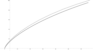
Figure 1. Comparison of $I_{(S^{3}\times{\mathbb{R}},2(g_{0}^{3}+dt^{2}))}(v)$ (dashed) and $0.886I_{(S^{5},7.85g_{0}^{5})}(v)$ (continuous) for $4\leq v\leq 65$.

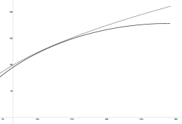
Figure 2. Comparison of $12.32v^{\frac{1}{2}}$ (dashed) and $(0.886)I_{(S^{5},7.85g_{0}^{5})}(v)$ (continuous) for $65\leq v\leq 291$.

We will make use of the following result from [25].

Lemma 3.5.

(Lemma 2.1 of [25]) For all $v\geq 0$

$$I_{(S^{2}\times{\mathbb{R}}^{2},g_{0}^{2}+dt^{2})}(v)\geq I_{(S^{3}\times{\mathbb{R}},2(g_{0}^{3}+dt^{2}))}(v)$$

We now prove the inequalities of Theorem 1.2. Recall that the isoperimetric profiles of $(S^{m},g_{0}^{m})$ and $(S^{m}\times{\mathbb{R}},g_{0}^{m}+dt^{2})$ are known (eqs. (15),(16) and (13),(14), respectively) so that comparisons with these profiles can be done through direct computations when needed. These will be shown on graphs.

We begin with the proof of inequality (3) of Theorem 1.2 in the next two lemmas.

Lemma 3.6.

For $v\leq 65$, $I_{(S^{2}\times{\mathbb{R}}^{2},g_{0}^{2}+dt^{2})}(v)\geq 0.886I_{(S^{4},4.7g_{0}^{4})}(v).$

Proof.

We will prove

(27) $$I_{(S^{3}\times{\mathbb{R}},2(g_{0}^{3}+dt^{2}))}(v)\geq 0.866I_{(S^{4},4.7g_{0}^{4})}(v)$$

for $v\leq 65$. The Lemma will then follow from inequality of Lemma 3.5.

By direct computation, $I_{(S^{3}\times{\mathbb{R}},2(g_{0}^{3}+dt^{2}))}(4)>(5.5)4^{\frac{3}{4}}$, which satisfies the hypothesis of Lemma 3.3. Hence, for $v\leq 4$:

$$I_{(S^{3}\times{\mathbb{R}},2(g_{0}^{3}+dt^{2}))}(v)>\frac{\gamma_{4}}{5.5}I_{(S^{4},4.7g_{0}^{4})}(v)>0.866I_{(S^{4},4.7g_{0}^{4})}(v).$$

Finally, for $4\leq v\leq 65$, inequality (27) can be checked by direct computations, since these isoperimetric profiles are known. We provide the graphics (see figure 1).

∎

Lemma 3.7.

For $v\geq 65$, $I_{(S^{2}\times{\mathbb{R}}^{2},g_{0}^{2}+dt^{2})}(v)\geq 0.886I_{(S^{4},4.7g_{0}^{4})}(v).$

Proof.

By direct computation, using equations (13) and (14)

$$I_{(S^{3}\times{\mathbb{R}},2(g_{0}^{3}+dt^{2}))}(65)\approx 99.4$$

So that $x_{0}=65$ and $y_{0}=99.4$ satisfy the hypothesis of Lemma 3.1, since

$$99.4\leq I_{(S^{3}\times{\mathbb{R}},2(g_{0}^{3}+dt^{2}))}(65)\leq I_{(S^{2}\times{\mathbb{R}}^{2},g_{0}^{2}+dt^{2})}(65)$$

Lemma 3.1, then yields

(28) $$12.32v^{\frac{1}{2}}\leq I_{(S^{2}\times{\mathbb{R}}^{2},g_{0}^{2}+dt^{2})}(v)$$

for $v\geq 65$. The isoperimetric profile of $(S^{4},4.7g_{0}^{4})$ is given by eqs. (15) and (16). Using direct computations we check that,

(29) $$0.886I_{(S^{4},5g_{0}^{4})}(v)<12.32v^{\frac{1}{2}}$$

for $v$, $65\leq v\leq 291$ (see figure 2). Note that at $\frac{25V_{4}}{2}\approx 290.69$, $I_{(S^{4},5g_{0}^{4})}(v)$ attains its maximum, while $12.32v^{\frac{1}{2}}$ is nondecreasing. This implies the inequality (29) is still valid even for $v\geq\frac{25V_{4}}{2}$. Inequalities (28) and (29) imply the Lemma. ∎

We will use the following results from [26].

Lemma 3.8.

(Corollary 3.2 of [26]) For all $v\geq 0$,

$$I_{(S^{3}\times{\mathbb{R}}^{2},(g_{0}^{2}+dt^{2}))}(v)\geq 0.99I_{(S^{4}\times{\mathbb{R}},2^{\frac{3}{2}}(g_{0}^{4}+dt^{2}))}(v)$$

Lemma 3.9.

(Lemma 4.1 of [26])

For all $v\geq 0$, we have $I_{(S^{2}\times{\mathbb{R}}^{3},(g_{0}^{2}+dt^{2}))}(v)\geq 0.99I_{(S^{4}\times{\mathbb{R}},2^{\frac{5}{3}}(g_{0}^{4}+dt^{2}))}(v).$

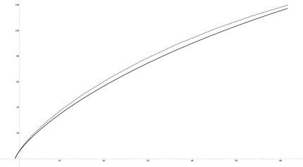
Figure 3. Comparison of $I_{(S^{4}\times{\mathbb{R}},2^{\frac{3}{2}}(g_{0}^{4}+dt^{2}))}(v)$ (dashed) and $(0.91)I_{(S^{5},2.77g_{0}^{5})}(v)$ (continuous) for $1\leq v\leq 60$.

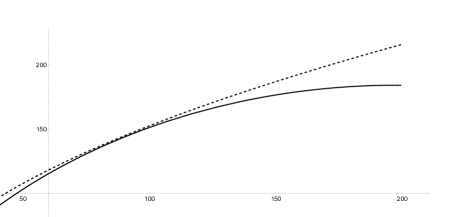
Figure 4. Comparison of $15.26v^{\frac{1}{2}}$ (dashed) and $(0.91)I_{(S^{5},2.77g_{0}^{5})}(v)$ (continuous) for $60\leq v\leq 200$.

We now prove inequalities (5) and (4) from Theorem 1.2.

Lemma 3.10.

For $v\geq 0$, $I_{(S^{3}\times{\mathbb{R}}^{2},(g_{0}^{2}+dt^{2}))}(v)\geq(0.91)I_{(S^{5},2.77g_{0}^{5})}(v).$

Proof.

Case 1: For $0\leq v\leq 1$.

By direct computation, $0.99I_{(S^{4}\times{\mathbb{R}},2^{\frac{3}{2}}(g_{0}^{4}+dt^{2}))}(1)>6.5.$ Which we use as hypothesis of Lemma 3.3, to obtain: for $0\leq v\leq v_{1}$,

(30) $$0.99I_{(S^{4}\times{\mathbb{R}},2^{\frac{3}{2}}(g_{0}^{4}+dt^{2}))}(v)>\frac{6.5}{\gamma_{5}}I_{(S^{5},2.77g_{0}^{5})}(v)>(0.91)I_{(S^{5},2.77g_{0}^{5})}(v).$$

From this and lemma 3.8, it follows that the lemma is satisfied for $v\leq 1$.

Case 2: For $1\leq v\leq 60$.

Since the isoperimetric profiles $I_{(S^{4}\times{\mathbb{R}},2^{\frac{3}{2}}(g_{0}^{4}+dt^{2}))}(v)$ and $I_{(S^{5},2.77g_{0}^{5})}(v)$ are known, it follows from direct computations that

$$0.99I_{(S^{4}\times{\mathbb{R}},2^{\frac{3}{2}}(g_{0}^{4}+dt^{2}))}(v)>(0.91)I_{(S^{5},2.77g_{0}^{5})}(v)$$

for $1\leq v\leq 60$, see figure 3. From this and lemma 3.8, the case is satisfied.

Case 3: For $v\geq 60$.

We have

$$I_{(S^{3}\times{\mathbb{R}}^{2},(g_{0}^{2}+dt^{2}))}(60)>0.99I_{(S^{4}\times{\mathbb{R}},2^{\frac{3}{2}}(g_{0}^{4}+dt^{2}))}(60)>118.245$$

where the first inequality follows from lemma 3.8, and the second from direct computation. We may then use $x_{0}=60$, $y_{0}=118.245$ as the hypothesis for lemma 3.1, and obtain, for $v\geq 60$, $I_{(S^{3}\times{\mathbb{R}}^{2},(g_{0}^{2}+dt^{2}))}(v)>15.26v^{\frac{1}{2}}.$

On the other hand, by direct computations (see figure 4), $15.26v^{\frac{1}{2}}>(0.91)I_{(S^{5},2.77g_{0}^{5})}(v)$, for $60\leq v\leq 200$. So that combined, these last two inequalities give, for $60\leq v\leq 200$,

(31) $$I_{(S^{3}\times{\mathbb{R}}^{2},(g_{0}^{2}+dt^{2}))}(v)>(0.91)I_{(S^{5},2.77g_{0}^{5})}(v)$$

Finally, we note that $I_{(S^{5},2.77g_{0}^{5})}(v)$ reaches its maximum at $v=\frac{Vol((S^{5},2.77g_{0}^{5}))}{2}\approx 198.4$, while $I_{(S^{3}\times{\mathbb{R}}^{2},(g_{0}^{2}+dt^{2}))}(v)$ is non-decreasing, by Lemma 3.1. This implies that eq. (31) is still valid for $v\geq 200$.

∎

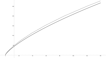
Figure 5. Comparison of $I_{(S^{4}\times{\mathbb{R}},2^{\frac{5}{3}}(g_{0}^{4}+dt^{2}))}(v)$ (dashed) and $(0.867)I_{(S^{5},7.5g_{0}^{5})}(v)$ (continuous) for $13\leq v\leq 140$.

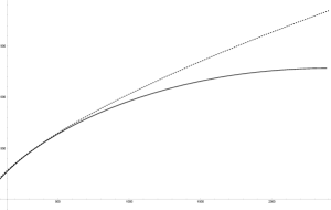
Figure 6. Comparison of $10.3v^{\frac{2}{3}}$ (dashed) and $(0.867)I_{(S^{5},7.5g_{0}^{5})}(v)$ (continuous) for $140\leq v\leq 2389$.

Lemma 3.11.

For $v\geq 0$, $I_{(S^{2}\times{\mathbb{R}}^{3},(g_{0}^{2}+dt^{2}))}(v)\geq 0.867I_{(S^{5},7.5g_{0}^{5})}(v)$.

Proof.

Case 1: For $0\leq v\leq 13$.

By direct computation $0.99I_{(S^{4}\times{\mathbb{R}},2^{\frac{5}{3}}(g_{0}^{4}+dt^{2}))}(13)>13^{\frac{4}{5}}(6.34)$, which we use as hypothesis of Lemma 3.3, to obtain: for $0\leq v\leq 13$,

(32) $$0.99I_{(S^{4}\times{\mathbb{R}},2^{\frac{5}{3}}(g_{0}^{4}+dt^{2}))}(v)>\frac{6.34}{\gamma_{5}}I_{(S^{5},7.5g_{0}^{5})}(v)>(0.867)I_{(S^{5},7.5g_{0}^{5})}(v)$$

From this and lemma 3.9, we conclude case 1.

Case 2: For $13\leq v\leq 140$.

Since the isoperimetric profiles $I_{(S^{4}\times{\mathbb{R}},2^{\frac{5}{3}}(g_{0}^{4}+dt^{2}))}(v)$ and $I_{(S^{5},7.5g_{0}^{5})}(v)$ are known, it follows from direct computations (see figure 5) that for $13\leq v\leq 140$,

$$0.99I_{(S^{4}\times{\mathbb{R}},2^{\frac{5}{3}}(g_{0}^{4}+dt^{2}))}(v)>(0.867)I_{(S^{5},7.5g_{0}^{5})}(v)$$

From this inequality and lemma 3.9, this case is satisfied.

Case 3: For $v\geq 140$.

By direct computation, $0.99I_{(S^{4}\times{\mathbb{R}},2^{\frac{3}{2}}(g_{0}^{4}+dt^{2}))}(140)>277.8$. Hence, by lemma 3.9: $I_{(S^{2}\times{\mathbb{R}}^{3},(g_{0}^{2}+dt^{2}))}(140)>277.8$. We then use $x_{0}=140$, $y_{0}=277.8$ as the hypothesis for Lemma 3.1 and get, for $v\geq 140$, $I_{(S^{2}\times{\mathbb{R}}^{3},(g_{0}^{2}+dt^{2}))}(v)>10.3v^{\frac{2}{3}}.$

Now, from direct computations (see figure 6), we have $10.3v^{\frac{2}{3}}>(0.867)I_{(S^{5},7.5g_{0}^{5})}(v)$, for $140\leq v\leq 2389$. Hence, we have, for $140\leq v\leq 2389$,

(33) $$I_{(S^{2}\times{\mathbb{R}}^{3},(g_{0}^{2}+dt^{2}))}(v)>(0.867)I_{(S^{5},7.5g_{0}^{5})}(v).$$

Finally, we note that $I_{(S^{5},2.77g_{0}^{5})}(v)$ reaches its maximum at $v=\frac{Vol((S^{5},7.5g_{0}^{5}))}{2}\approx 2388.21$, while $I_{(S^{2}\times{\mathbb{R}}^{3},(g_{0}^{2}+dt^{2}))}(v)$ is non decreasing, by Lemma 3.1. This implies that inequality (33) is still valid for $v\geq 2389$.

∎

Lemmas 3.6, 3.7, 3.10, 3.11 imply Theorem 1.2.

Corollary 1.3 follows immediately from Theorem 1.2 in this article and Theorem 1.1 in [26]. We note that $I_{(M^{m}\times{\mathbb{R}}^{n},g+dx^{2})}$ is non-decreasing, by Lemma 3.1.

Theorem 3.12.

(Theorem 1.1 in [26]) Let $(M^{m},g)$ be a closed Riemannian manifold with scalar curvature $s_{g}\geq m(m-1)$. If $I_{(M^{m}\times{\mathbb{R}}^{n},g+dx^{2})}$ is a non-decreasing function and $I_{(M^{m}\times{\mathbb{R}}^{n},g+dx^{2})}\geq\lambda I_{(S^{n+m},\mu g_{0}^{m+n})}$, then

$$Y(S^{m}\times{\mathbb{R}}^{n},[g+dx^{2}])\geq min\left\{\frac{\mu m(m-1)}{(m+n)(m+n-1)},\lambda^{2}\right\}Y(S^{m+n})$$

We also recall Theorem 1.1 in [1]:

Theorem 3.13.

(Theorem 1.1 in [1]) Let $(M^{m},g)$ be a closed Riemannian m-manifold $(m\geq 2)$ of positive scalar curvature and $(N^{n},h)$ any Riemannian closed n-manifold $n\geq 2$: Then,

$$\lim_{r\rightarrow\infty}Y(M\times{\mathbb{R}}^{n},[g+rh])=Y(M\times{\mathbb{R}}^{n},[g+g_{E}])$$

Corollary 1.4 follows immediately from Corollary 1.3 and Theorem 1.1 in [1], by noting that

$$Y(M\times N)\geq\sup_{\{r>0\}}Y(M\times N,[g+rh])\geq\lim_{r\rightarrow\infty}Y(M\times{\mathbb{R}}^{n},[g+rh])=Y(M\times{\mathbb{R}}^{n},[g+g_{E}]).$$

References

[1] K. Akutagawa, L. Florit, J. Petean, On Yamabe constants of Riemannian
products, Comm. Anal. Geom. 15 (2007), 947-969.
[2] Akutagawa, K., Neves, A. 3-manifolds with Yamabe invariant greater than that of . J. Differential Geom.75, 359–386 (2007)
[3] F. J. Almgren, Spherical symmetrization, Proc. International workshop on integral functions
in the calculus of variations, Trieste 1985, Red. Circ. Mat. Palermo (2) Supple. (1987), 11-25.
[4] B. Ammann, M. Dahl, and E. Humbert, Smooth Yamabe invariant and surgery, J. Differ. Geom. 94
(2013), 1–58.
[5] B. Ammann, M. Dahl, and E. Humbert, Low-dimensional surgery and the Yamabe invariant,J. Math. Soc. Japan Vol. 67, No. 1 (2015) pp. 159–182
[6] D. Andreucci and A. F. Tedeev. Some remarks on the sobolev inequality on Riemannian manifolds. Proc. Amer. Math. Soc. 150 (2022), 1657-1667.
[7] D. Andreucci and A. F. Tedeev.Asymptotic Properties of Solutions to the Cauchy Problem for Degenerate Parabolic Equations with Inhomogeneous Density on Manifolds. Milan Journal of Mathematics volume 89 (2021), 295–327.
[8] T. Aubin, Equations differentielles non-lineaires et
probleme de Yamabe concernant la courbure scalaire,
J. Math. Pures Appl. 55 (1976), 269-296.
[9] V. Bayle, Propriétés du concavité du profil isopérimétrique et applications. Ph.D. Thesis, p. 52 (2004)
[10] E. Gonzalez, U. Massari and I. Tamanini, On the regularity of boundaries of sets minimizing
perimeter with a volume constraint, Indiana Univ. Math. J. 32 (1983), 25-37.
[11] J. Gonzalo, Large soap bubbles and isoperimetric regions in the product of Euclidean space with closed manifold. Ph. D. Thesis, University of California, Berkeley.
[12] Gursky, M., LeBrun, C. Yamabe invariants and Spinc structures. Geom. Funct. Anal. 8, 965–977 (1998)
[13] Kobayashi, O.On large scalar curvature Research Report 11. Dept. Math. Keio Univ. (1985)
[14] LeBrun, C. The Scalar Curvature of 4-Manifolds. In Perspectives in Scalar Curvature, Volume 1, edited by M.L. Gromov and H.B. Lawson Jr., pp. 643-707. World Scientific. (2023)
[15] F. Morgan, Geometric measure theory: a beginner’s guide, 2nd ed., Academic Press, 1998.
[16] F. Morgan. Isoperimetric estimates in products, Ann. Glob. Anal. Geom. 30 (2006) , 73-79.
[17] F. Morgan. Isoperimetric balls in cones over tori, 35 Ann. Glob. Anal. Geom. (2009) 133–137
[18] F. Morgan, M. Ritoré, Isoperimetric regions in cones. Trans. Am. Math. Soc. 354, (2002) 2327–2339
[19] M. Grüter, Boundary regularity for solutions of a partitioning problem, Arch. Rat. Mech. Anal. 97 (1987), 261-270.
[20] T. H. Parker and J. M. Lee, The Yamabe Problem, Bull. of the Amer. Math. Soc. 17, Number 1, (1987), 37-91.
[21] R. Pedrosa, The isoperimetric problem in spherical cylinders. Ann. Global Anal. Geom. 26 (2004), 333-354.
[22] R. Pedrosa, M. Ritoré, Isoperimetric domains in the Riemannian product of a circle with a simply connected space form and applications to free boundary problems, Indiana Univ. Math. J.
48 (1999), 1357-1394.
[23] Petean, J. Best Sobolev constants and manifolds with positive scalar curvature metrics. Ann. Global
Anal. Geom. 20, 231–242 (2001)
[24] J. Petean, Isoperimetric regions in spherical cones and Yamabe constants of . Geom Dedicata 143, 37 (2009) 37-48
[25] J. Petean and J. M. Ruiz, Isoperimetric profile comparisons and Yamabe constants. Ann. Glob. Anal. Geom. Vol. 40, No. 2, (2011). 177-189.
[26]J. Petean and J. M. Ruiz, On the Yamabe constants of
and , Differential Geometry and its Applications
31 (2), (2013) 308-319
[27] M. Ritoré, and E. Vernadakis, Large isoperimetric regions in the product of a compact manifold with Euclidean space, Advances in Mathematics. 306, (2017) 958-972.
[28] A. Ros. The isoperimetric problem, Global Theory of Minimal Surfaces (Proc. Clay Math. Institute Summer School, 2001). Amer. Math. Soc., Providence. (2005)
[29] J. M. Ruiz and A. Vázquez Juárez, Isoperimetric estimates in low dimensional Riemannian products Ann. Glob. Anal Geom 59, 417–434 (2021).
[30] R. Schoen, Conformal deformation of a Riemannian metric to constant scalar curvature, J. Differ. Geom. 20 (2) (1984),
479-495.
[31] R. Schoen, Variational theory for the total scalar curvature functional for Riemannian metrics and related topics. In: Lectures Notes in Math, vol 1365, pp. 120–154. Springer-Verlag, Berlin (1989)
[32] N. Trudinger,
Remarks concerning the conformal deformation of Riemannian
structures on compact manifolds, Ann. Scuola Norm. Sup. Pisa
22 (1968), 265-274.
[33] C. Viana The isoperimetric problem for lens spaces, Mathematische Annalen 374 (2019) 475–497
[34] H. Yamabe, On a deformation of Riemannian
structures on compact manifolds, Osaka Math. J. 12 (1960),
21-37.