Dynamic structure factor of two-dimensional Fermi superfluid with Rashba spin-orbit coupling

Abstract

We theoretically calculate the dynamic structure factor of two-dimensional Rashba-type spin-orbit coupled (SOC) Fermi superfluid with random phase approximation, and analyze the main characters of dynamical excitation shown by both density and spin dynamic structure factor during a continuous phase transition between Bardeen-Cooper-Schrieffer superfluid and topological superfluid. Generally we find three different excitations, including collective phonon excitation, two-atom molecular and atomic excitations, and pair-breaking excitations due to two-branch structure of quasi-particle spectrum. It should be emphasized that collective phonon excitation is overlapped with a gapless $DD$ type pair-breaking excitation at the critical Zeeman field $h_{c}$, and is imparted a finite width to phonon peak when transferred momentum q is around Fermi vector $k_{F}$. At a much larger transferred momentum ($\textbf{{q}}=4k_{F}$), the pair-breaking excitation happens earlier than two-atom molecular excitation, which is different from the conventional Fermi superfluid without SOC effect.

I Introduction

Finding and distinguishing exotic matter states are interesting and important tasks in quantum many-body physics (Bloch2008rmp, ; Giorgini2008rmp, ). In atomic physics, the strategy that analyzing the atomic spectrum structure shown by all possible electronic transition between atomic energy levels has been verified to be an effective way to distinguish chemical elements. All spectra consist of dynamical excitations information, which can be described by optical spectrum dynamic structure factor. In quantum many-body physics, many particles interplay with each other and arrive at rich equilibrium matter states. Since the realization of spin-linear (angular) momentum coupling effect in ultracold atomic gases (Lin2011s, ; Wang2012s, ; Cheuk2012s, ; Chen2018prl, ; Zhang2019prl, ; Williams2013, ; Meng2016, ; Burdick2016, ; Huang2016, ; Wu2016, ; Wang2021, ), it has been possible to investigate many exotic matter states, such as two types of stripe phase with discrete translational or rational symmetry (Ho2011b, ; Michael2015pra, ; Qu2015pra, ), the topological state (Jiang2011m, ; Chen2022prr, ; Han2023, ), etc., in these highly controllable systems. Naturally it is interesting to know whether it is possible to find a universal way to identify all these matter states with dynamical excitations information.

Dynamic structure factor, which is related to the imaginary part of response function in the momentum-energy representation, is an important many-body physical quantity and includes rich dynamics about the system in a certain matter state (Pitaevskii2003book, ). Experimentally dynamic structure factor can be measured by a two-photon Bragg scattering technique (Veeravalli2008b, ; Hoinka2017g, ; Biss2022, ; Senaratne2022, ; Pagano2014, ), in which two Bragg laser beams can transfer a selected transferred momentum q and energy $\omega$ to perturb the system. After this Bragg perturbation, the dynamic structure factor can be obtained by measuring the centre-of-mass velocity of the system (Brunello2001pra, ). In a small transferred momentum q, some momentum-related collective modes, like Goldstone phonon (Hoinka2017g, ; Combescot2006pra, ; Kettmann2017, ), second sound (Hu2022aapps, ; Li2022, ), Higgs mode (Pekker2015arcmp, ; Behrle2018, ; Bjerlin2016, ; Bruun2014, ; Zhao2020d, ; Fan2022p, ; Phan2023, ), and Leggett excitation (Leggett1966n, ; Zhang2017t, ), can be observed. At a large q, the dynamics is dominated by the single-particle excitation, including not only the Cooper pair-breaking excitation, but also the ideal (or interaction-revised) atomic or molecular excitation (Combescot2006m, ; Combescot2006pra, ). All these dynamics consist of dynamical character of the system in a specific matter state, and may display different dynamical behaviours during phase transition. So it is interesting to study these dynamical characters of the system in different matter states according to dynamic structure factor, and check the feasibility to identify matter state by dynamic structure factor. In our previous work, dynamic structure factor had been found that it can display different dynamical behaviours in a few phase transitions (Zou2021d, ; Gao2023pra, ; Han2022, ).

In this paper, we theoretically investigate a two-dimensional (2D) Rashba-type spin-orbit coupled (SOC) Fermi superfluid, which can experience a continuous phase transition between a conventional Bardeen-Cooper-Schrieffer (BCS) superfluid to a topological superfluid by continuously varying the Zeeman field (Liu2012praR, ). We numerically calculate dynamic structure factor of this system with random phase approximation (AndersonPR1958, ; Liu2004c, ), and try to find its main dynamical excitation character during phase transition. We find the dynamic structure factor presents rich excitation signals, including collective phonon excitation, molecular or atomic excitations, and four kinds of pair-breaking excitations due to two-branch structure of quasi-particle spectrum. Among all these excitations, the collective phonon excitation requires the smallest excitation energy in both the BCS and topological superfluid. In the critical point of phase transition, one of pair-breaking excitations becomes gapless excitation. It overlaps with the phonon excitation and imparts a finite expansion width to the phonon peak in a certain transferred momentum. This paper is organized as follows. In the next section, we will use the motion equation of Green’s function to introduce the microscopic model of a 2D Fermi superfluid with the Rashba SOC effect, outline the mean-field approximation, and show how to calculate the response function with the random phase approximation. We give results of the dynamic structure factor of both BCS and topological superfluids in Sec. III, and give our conclusions and outlook in Sec. IV. Some calculation details will be listed in the Appendix.

II Methods

II.1 Model and Hamiltonian

We consider a uniform 2D Fermi gases subject to a Rashba SOC potential $V_{{\rm soc}}=-i\lambda\left(\partial_{y}+i\partial_{x}\right)$ with strength $\lambda$ and a Zeeman field $h$. The system can be described by a model Hamiltonian

$$H=\int d^{2}r\left[\sum_{\sigma}\mathcal{H}_{\sigma}^{S}+\mathcal{H}_{{\rm SOC}}+\mathcal{H}_{{\rm int}}\right].$$ (1)

Here $\mathcal{H}_{\sigma}^{S}=\psi_{\sigma}^{\dagger}\left[-\nabla^{2}/2m-\mu-h\sigma_{z}\right]\psi_{\sigma}$ is the single particle Hamiltonian of spin-$\sigma$ component particles with mass $m$ in reference to the chemical potential $\mu$, and $\psi_{\sigma}(\psi_{\sigma}^{\dagger})$ is the annihilation (generation) operator. $\mathcal{H}_{{\rm SOC}}=\psi_{\uparrow}^{\dagger}V_{{\rm soc}}\psi_{\downarrow}+h.c.$ is the Rashba SOC Hamiltonian, and it should be noted that the strength $\lambda$ of SOC effect is isotropic in the 2D $XY$-plane. $\mathcal{H}_{{\rm int}}=U\psi_{\uparrow}^{\dagger}\psi_{\downarrow}^{\dagger}\psi_{\downarrow}\psi_{\uparrow}$ describes the contact interaction between opposite spins, in which the strength $U$ should be regularized via $1/U=-\sum_{\textbf{{k}}}1/\left(\textbf{{k}}^{2}/m+E_{a}\right)$. $E_{a}$ is the binding energy of the two-body bound state, and is often used to demonstrate the interaction strength in 2D system (Bertaina2011PRL, ). Here and in the following we have set $\hbar=k_{B}=1$ for simple. Since we consider a uniform system with bulk density $n_{0}$, the inverse of Fermi wave vector $k_{F}=\sqrt{2\pi n_{0}}$ and Fermi energy $E_{F}=k_{F}^{2}/2m$ are used as length and energy units, respectively.

A standard mean-field treatment is carried out to the interaction Hamiltonian $\mathcal{H}_{{\rm int}}$ with the usual definition of order parameter $\Delta=-U\left\langle\psi_{\downarrow}\psi_{\uparrow}\right\rangle$. After Fourier transformation to the mean-field model Hamiltonian, we can obtain its expression in the momentum representation, which reads

$$\begin{array}[]{cl}H_{{\rm mf}}&=\underset{\textbf{{k}}\sigma}{\sum}\left(\xi_{\textbf{{k}}}-h\sigma_{z}\right)c_{\textbf{{k}}\sigma}^{\dagger}c_{\textbf{{k}}\sigma}\\ &+\underset{\textbf{{k}}}{\sum}\left[\lambda\left(k_{y}+ik_{x}\right)c_{\textbf{{k}}\uparrow}^{\dagger}c_{\textbf{{k}}\downarrow}+h.c.\right]\\ &-\underset{\textbf{{k}}}{\sum}\left[\Delta c_{\textbf{{k}}\uparrow}^{\dagger}c_{-\textbf{{k}}\downarrow}^{\dagger}+\Delta^{*}c_{-\textbf{{k}}\downarrow}c_{\textbf{{k}}\uparrow}\right]\end{array}$$ (2)

with $\xi_{\textbf{{{{k}}}}}=\textbf{{k}}^{2}/2m-\mu$. Usually the order parameter $\Delta$ is a complex number. However U(1) symmetry is spontaneously broken in the ground state of the system, and the value for the phase of $\Delta$ is pushed to choose a random number. Here we just set $\Delta=\Delta^{*}$. The exact diagonalization of mean-field Hamiltonian $H_{{\rm mf}}$ can be solved with motion equation of Green’s functions. Finally we get six independent Green’s functions, which are

$$\begin{array}[]{ccc}G_{1}\left(\textbf{{k}},\omega\right)&\equiv\left\langle\left\langle c_{\textbf{{k}}\uparrow}|c_{\textbf{{k}}\uparrow}^{\dagger}\right\rangle\right\rangle&=\underset{l}{\sum}\left[G_{1}\right]_{\textbf{{k}}}^{l}/\left(\omega-E_{\textbf{{k}}}^{l}\right),\\ G_{2}\left(\textbf{{k}},\omega\right)&\equiv\left\langle\left\langle c_{\textbf{{k}}\downarrow}|c_{\textbf{{k}}\downarrow}^{\dagger}\right\rangle\right\rangle&=\underset{l}{\sum}\left[G_{2}\right]_{\textbf{{k}}}^{l}/\left(\omega-E_{\textbf{{k}}}^{l}\right),\\ \varGamma\left(\textbf{{k}},\omega\right)&\equiv\left\langle\left\langle c_{\textbf{{k}}\uparrow}|c_{-\textbf{{k}}\downarrow}\right\rangle\right\rangle&=\underset{l}{\sum}\left[\varGamma\right]_{\textbf{{k}}}^{l}/\left(\omega-E_{\textbf{{k}}}^{l}\right),\\ S\left(\textbf{{k}},\omega\right)&\equiv\left\langle\left\langle c_{\textbf{{k}}\downarrow}|c_{\textbf{{k}}\uparrow}^{\dagger}\right\rangle\right\rangle&=\underset{l}{\sum}\left[S\right]_{\textbf{{k}}}^{l}/\left(\omega-E_{\textbf{{k}}}^{l}\right),\\ F_{1}\left(\textbf{{k}},\omega\right)&\equiv\left\langle\left\langle c_{\textbf{{k}}\uparrow}|c_{-\textbf{{k}}\uparrow}\right\rangle\right\rangle&=\underset{l}{\sum}\left[F_{1}\right]_{\textbf{{k}}}^{l}/\left(\omega-E_{\textbf{{k}}}^{l}\right),\\ F_{2}\left(\textbf{{k}},\omega\right)&\equiv\left\langle\left\langle c_{\textbf{{k}}\downarrow}|c_{-\textbf{{k}}\downarrow}\right\rangle\right\rangle&=\underset{l}{\sum}\left[F_{2}\right]_{\textbf{{k}}}^{l}/\left(\omega-E_{\textbf{{k}}}^{l}\right),\end{array}$$ (3)

where $l=\pm 1,\pm 2$ denotes respectively all four important quasi-particle energy spectra $E_{\textbf{{k}}}^{\left(+1\right)}=-E_{\textbf{{k}}}^{\left(-1\right)}=U_{\textbf{{k}}}$ and $E_{\textbf{{k}}}^{\left(+2\right)}=-E_{\textbf{{k}}}^{\left(-2\right)}=D_{\textbf{{k}}}$. $U_{\textbf{{k}}}$ and $D_{\textbf{{k}}}$ are respectively the up- and down-branch positive quasi-particle spectrum

$$U_{\textbf{{k}}}=\sqrt{E_{\textbf{{k}}}^{2}+h^{2}+\textbf{{k}}^{2}\lambda^{2}+2\sqrt{E_{\textbf{{k}}}^{2}h^{2}+\xi_{\textbf{{k}}}^{2}\textbf{{k}}^{2}\lambda^{2}}},$$ (4)

$$D_{\textbf{{k}}}=\sqrt{E_{\textbf{{k}}}^{2}+h^{2}+\textbf{{k}}^{2}\lambda^{2}-2\sqrt{E_{\textbf{{k}}}^{2}h^{2}+\xi_{\textbf{{k}}}^{2}\textbf{{k}}^{2}\lambda^{2}}},$$ (5)

with $E_{\textbf{{k}}}=\sqrt{\xi_{\textbf{{k}}}^{2}+\Delta^{2}}$. The Green’s functions $S,F_{1}$and $F_{2}$ come from the Rashba SOC Hamiltonian, and they are the odd functions of momentum k, which are the even functions in the Raman SOC case. These single-particle spectra ($U_{\textbf{{k}}}$ and $D_{\textbf{{k}}}$) do great influence to the static and dynamical properties of ground state. All expressions related to $\left[G_{1}\right]_{\textbf{{k}}}^{l}$,$\left[G_{2}\right]_{\textbf{{k}}}^{l}$,$\left[\Gamma\right]_{\textbf{{k}}}^{l}$,$\left[S\right]_{\textbf{{k}}}^{l}$,$\left[F_{1}\right]_{\textbf{{k}}}^{l}$ and $\left[F_{2}\right]_{\textbf{{k}}}^{l}$ will be given in the appendix.

Based on the spectrum theorem, it is also easy to get all equations of all physical quantities with the above Green’s functions. For example, we obtain spin-up and spin-down density equations

$$n_{1}=\sum_{\textbf{{k}}}\left\langle c_{\textbf{{k}}\uparrow}^{\dagger}c_{\textbf{{k}}\uparrow}\right\rangle=-\frac{1}{\pi}\sum_{\textbf{{k}}}\int d\omega\frac{{\rm Im}\left[G_{1}\left(\textbf{{k}},\omega\right)\right]}{e^{\omega/T}+1},$$ (6)

$$n_{2}=\sum_{\textbf{{k}}}\left\langle c_{\textbf{{k}}\downarrow}^{\dagger}c_{\textbf{{k}}\downarrow}\right\rangle=-\frac{1}{\pi}\sum_{\textbf{{k}}}\int d\omega\frac{{\rm Im}\left[G_{2}\left(\textbf{{k}},\omega\right)\right]}{e^{\omega/T}+1},$$ (7)

and order parameter equation

$$\frac{\Delta}{U}=-\sum_{\textbf{{k}}}\left\langle c_{-\textbf{{k}}\downarrow}c_{\textbf{{k}}\uparrow}\right\rangle=\frac{1}{\pi}\sum_{\textbf{{k}}}\int d\omega\frac{{\rm Im}\left[\varGamma\left(\textbf{{k}},\omega\right)\right]}{e^{\omega/T}+1},$$ (8)

with Green’s function $G_{1}$, $G_{2}$ and $\varGamma$ in Eq. 3 at the temperature $T$. By self-consistently solving the density and order parameter equations, the value of chemical potential $\mu$ and order parameter $\Delta$ can be numerically calculated.

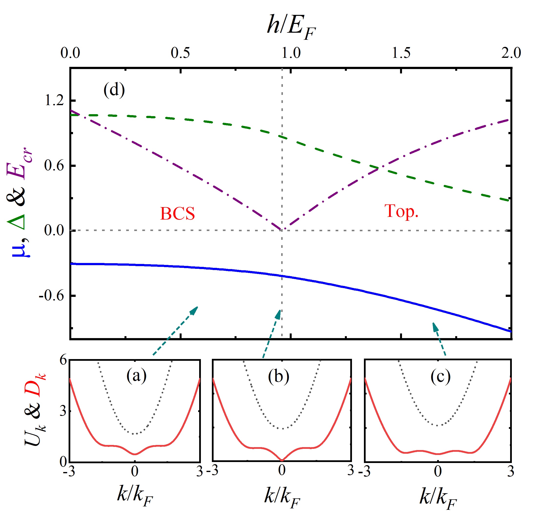
Figure 1: Two types of single-particle excitation spectra $U_{\textbf{{k}}}$ (black short-dotted line) and $D_{\textbf{{k}}}$ (red solid line) at different Zeeman field (a) $h=0.6E_{F}$, (b) $h=0.96E_{F}$ and (c) $h=1.3E_{F}$. (d) The distribution of chemical potential (blue solid line), order parameter (olive dashed line) and $E_{{\rm cr}}=\left|h-\sqrt{\mu^{2}+\Delta^{2}}\right|$ (purple dash-dotted line) at different Zeeman field $h$ during a continuous phase transition between BCS superfluid and topological superfluid. A gray vertical dotted line marks the location of a critical value of Zeeman field $h_{c}=0.96E_{F}$ at $E_{a}=0.5E_{F}$ and $\lambda k_{F}/E_{F}=1.5$.

In this paper, we just consider the zero temperature case and take the binding energy $E_{a}=0.5E_{F}$ and SOC strength $\lambda k_{F}/E_{F}=1.5$. As shown in Fig. 1, the system experiences a phase transition from BCS superfluid to topological superfluid by increasing the Zeeman field $h$ over a critical value $h_{c}=0.96E_{F}$. This is a continuous phase transition, which are displayed by the smooth variation of chemical potential $\mu$ and order parameter $\Delta$ with Zeeman field $h$. The critical Zeeman field $h_{c}$ is determined by the zero value of $E_{{\rm cr}}=\left|h-\sqrt{\mu^{2}+\Delta^{2}}\right|$, and also in which the minimum of $D_{\textbf{{k}}}$ touches zero at momentum $\textbf{{k}}=0$ ( red line of panel (b) in Fig. 1). During this continuous phase transition from BCS superfluid to topological one, the value of the second-order local minimum in lower-branch spectrum $D_{\textbf{{k}}}$ at a non-zero momentum k will experience a variation from the situation that much larger than the global minimum at $\textbf{{k}}=0$ in the BCS regime, then to the case almost the same value of the global one at $\textbf{{k}}=0$ in the topological regime, while the spectrum structure of $U_{\textbf{{k}}}$ does not change too much. We have also checked that this continuous phase transition will be present in a quite large parameter space of SOC strength $\lambda$, except a weak SOC strength $\lambda k_{F}/E_{F}<0.4$ where the parameter space of topological superfluid is depressed to almost vanish and make the phase transition to be a first order one from a trivial superfluid to normal state.

Next we will discuss the dynamical excitation of this system.

II.2 Response function and random phase approximation

At zero temperature, the interacting system comes into a superfluid state and induces four different densities. Besides the normal spin-up density $n_{1}=\left\langle\psi_{\uparrow}^{\dagger}\psi_{\uparrow}\right\rangle$ and spin-down density $n_{2}=\left\langle\psi_{\downarrow}^{\dagger}\psi_{\downarrow}\right\rangle$, the pairing physics of two spins generates the other anomalous density $n_{3}=\left\langle\psi_{\downarrow}\psi_{\uparrow}\right\rangle$ and its conjugate counterpart $n_{4}=\left\langle\psi_{\uparrow}^{\dagger}\psi_{\downarrow}^{\dagger}\right\rangle$. The interaction between particles makes these four densities couple closely with each other. Any fluctuation in each kind of density will influence other densities and generate a non-negligible density fluctuation of them. This physics plays a significant role in the dynamical excitation of the system, which demonstrates the importance and necessity of the term in Hamiltonian beyond mean-field theory. Random phase approximation has been verified to be a good way to treat the fluctuation term of Hamiltonian (AndersonPR1958, ). Comparing with experiments, it can even obtain some quantitatively reliable predictions in three-dimensional Fermi superfluid (Zou2010q, ; Zou2018l, ). Its prediction also qualitatively agrees with quantum Monte Carlo data in 2D Fermi system (Zhao2020d, ; Vitali2017, ). Random phase approximation treats the fluctuation of Hamiltonian as parts of an effective external potential (Gao2023pra, ; Liu2004c, ), and find the response function $\chi$ of the system is connected to its mean-field approximation $\chi^{0}$, whose calculation is relatively easier, by the following equation

$$\chi=\frac{\chi^{0}}{1-\chi^{0}M_{I}U},$$ (9)

where

$$M_{I}=\left[\begin{array}[]{cccc}0&1&0&0\\ 1&0&0&0\\ 0&0&0&1\\ 0&0&1&0\end{array}\right]$$

is a constant matrix reflecting the coupling situation of four kinds of densities.

Next we introduce the expression of the mean-field response function $\chi^{0}$, which is a $4\times 4$ matrix

$$\chi^{0}=\left[\begin{array}[]{cccc}\chi_{11}^{0}&\chi_{12}^{0}&\chi_{13}^{0}&\chi_{14}^{0}\\ \chi_{21}^{0}&\chi_{22}^{0}&\chi_{23}^{0}&\chi_{24}^{0}\\ \chi_{31}^{0}&\chi_{32}^{0}&\chi_{33}^{0}&\chi_{34}^{0}\\ \chi_{41}^{0}&\chi_{42}^{0}&\chi_{43}^{0}&\chi_{44}^{0}\end{array}\right].$$ (10)

Here its $ij$ matrix element is defined by $\chi_{ij}^{0}\left(\textbf{{r}}_{1},\textbf{{r}}_{2},\tau,0\right)\equiv-\left\langle\hat{n}_{i}\left(\textbf{{r}}_{1},\tau\right)\hat{n}_{j}\left(\textbf{{r}}_{2},0\right)\right\rangle$, where density operators $\hat{n}_{i}$ and $\hat{n}_{j}$ had been introduced at the beginning of this sub-section. In the uniform system, all response function elements are only the function of 2D relative coordinate $\textbf{{r}}=\textbf{{r}}_{1}-\textbf{{r}}_{2}$ and time $\tau$. So a generalized coordinate $R=\left(\textbf{{r}},\tau\right)$ is used to go on discussing. Based on Wick’s theorem, we should consider all possible two-operators contraction terms, which are all related to 6 independent Green’s functions of Eq. 3. We find that the mean-field response function $\chi^{0}=A+B$, in which $A$ is only connected to Green’s functions $G_{1}$ , $G_{2}$ and $\Gamma$, while $B$ is connected the SOC Green’s functions $S$, $F_{1}$ and $F_{2}$. For example, in the spatial and time representation, $\chi_{11}^{0}\left(R\right)\equiv-\left\langle\hat{n}_{1}\left(\textbf{{r}}_{1},\tau\right)\hat{n}_{1}\left(\textbf{{r}}_{2},0\right)\right\rangle=A_{11}\left(R\right)+B_{11}\left(R\right)$, where $A_{11}\left(R\right)=G_{1}\left(-R\right)G_{1}\left(R\right)$ and $B_{11}\left(R\right)=-F_{1}^{*}\left(-R\right)F_{1}\left(R\right)$. After Fourier transformation to Green’s functions, we obtain the expression of all matrix elements in the momentum-energy representation

$$\chi^{0}\left(\textbf{{q}},\omega\right)=A\left(\textbf{{q}},\omega\right)+B\left(\textbf{{q}},\omega\right)$$ (11)

where

$$A=\left[\begin{array}[]{cccc}A_{11},&A_{12},&A_{13},&A_{14}\\ A_{12},&A_{22},&A_{23},&A_{24}\\ A_{14},&A_{24},&-A_{12},&A_{34}\\ A_{13},&A_{23},&A_{43},&-A_{12}\end{array}\right]$$

has 9 independent matrix elements, and

$$B=\left[\begin{array}[]{cccc}B_{11},&B_{12},&B_{13},&B_{14}\\ B_{21},&B_{22},&B_{23},&B_{24}\\ B_{31},&B_{32},&B_{33},&B_{34}\\ B_{41},&B_{42},&B_{43},&B_{44}\end{array}\right].$$

All expressions of these matrix elements are listed in the final appendix. The numerical calculation of above all matrix elements required a two-dimensional integral, which makes the numerical calculations here much heavier than the one-dimensional SOC system (Gao2023pra, ).

II.3 Dynamic structure factor

With Eqs. 9 and 11, we can obtain expression of both the total density response function $\chi_{n}\equiv\chi_{11}+\chi_{22}+\chi_{12}+\chi_{21}$ and spin density response function $\chi_{s}\equiv\chi_{11}+\chi_{22}-\chi_{12}-\chi_{21}$. $\chi_{n}$ reflects the density response of the system, while $\chi_{s}$ shows the spin density response in two-spin components. Based on the fluctuation and dissipation theorem, their imaginal parts are connected to density and spin dynamic structure factor by

$$S_{n/s}=-\frac{1}{\pi}\frac{1}{1-e^{-\omega/T}}{\rm Im}\left[\chi_{n/s}\right].$$ (12)

III Results

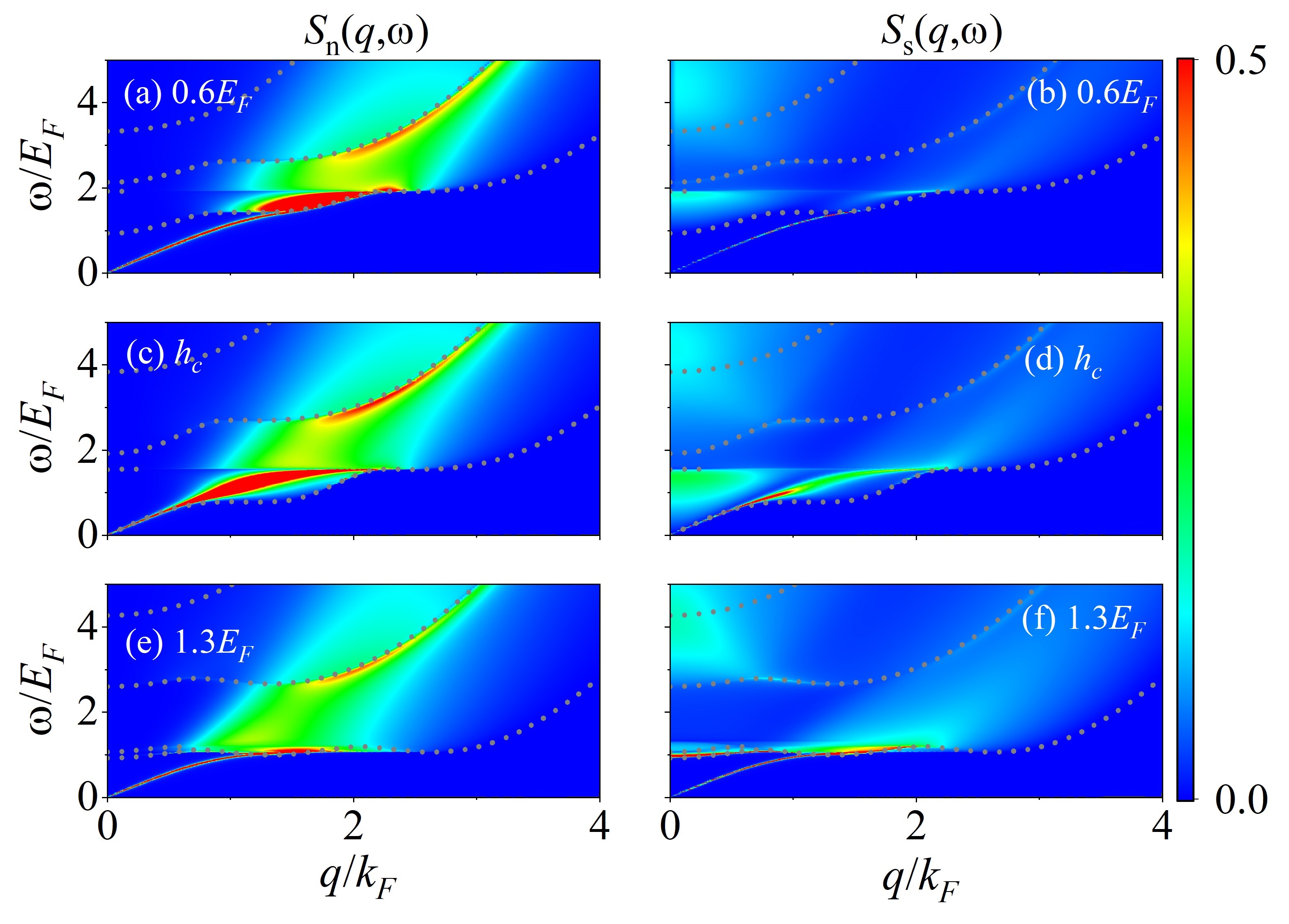
Figure 2: The density (left column) and spin (right column) dynamic structure factor at three typical different Zeeman fields $h=0.6E_{F},h_{c},1.3E_{F}$. The dotted lines are the same lines of Fig. 4, which reflects all kinds of threshold energy to break a Cooper pair.

In the following discussions, we focus on an interaction binding energy $E_{a}=0.5E_{F}$ and a typical SOC strength $\lambda k_{F}/E_{F}=1.5$ at zero temperature. These parameters are the same as one in Fig. 1. As introduced before, the isotropy of the Rashba SOC effect induces that the Hamiltonian Eq. 1 is also isotropic, which means the direction of the transferred momentum q can make no difference to the dynamical excitation of the system, so we just set q along the positive direction of $X$-axis. And the dynamical excitation of the system is also rotation-invariant in the 2D $XY$-plane.

We numerically calculate the density (left column) and spin (right column) dynamic structure factors, as shown in Fig. 2, in the phase transition from BCS superfluid (higher two panels), cross the critical regime (middle two panels), and then to topological superfluid (lower two panels). Generally we investigate a full dynamical excitation in different transferred momenta q, including the low energy (or momentum) collective excitation and the high energy (or momentum) single-particle excitation. The white dotted lines mark the location of three types of the minimum energy to break a Cooper pair, which will be introduced later.

III.1 Collective and single-particle excitation

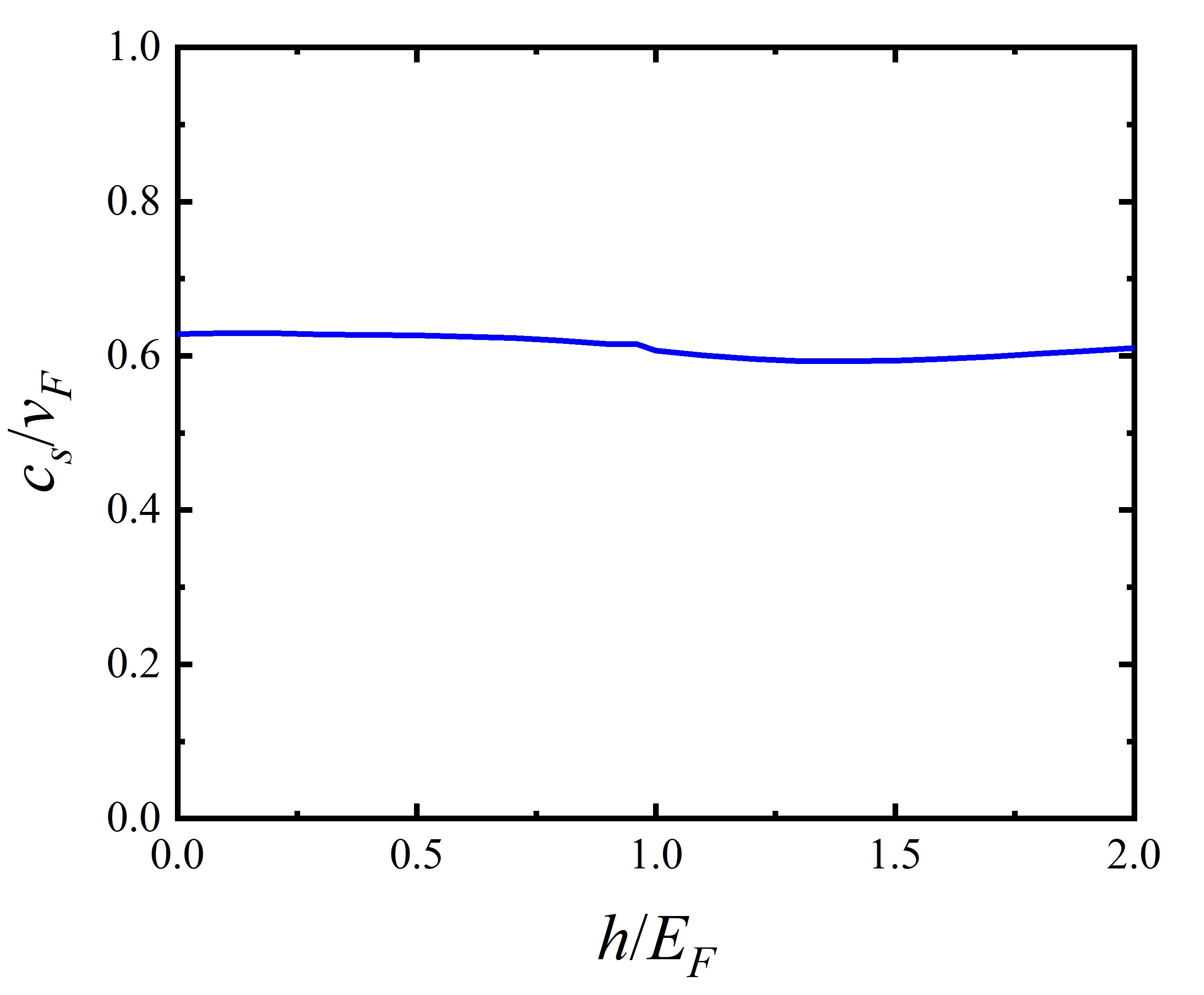
Figure 3: The sound velocity $c_{s}$ at different Zeeman field $h$.

At a low transferred energy $\omega$, it is easy to investigate the collective excitation (He2013aop, ). By continuously increasing transferred momentum q from zero, we initially see a gapless phonon excitation in both the density and spin dynamic structure factor. As shown in Fig. 3, the velocity of collective phonon excitation almost does not change during this continuous phase transition, which is different from the first order one in 1D Raman SOC Fermi superfluid (Gao2023pra, ). When the transferred momentum q is large enough, this phonon excitation gradually merges into the continuous single-particle excitation. Specially in the critical regime $h=h_{c}$, the minimum of lower single-particle spectrum $D_{\textbf{{k}}}$ touches zero (panel (b) of Fig. 1), which induces that a gapless pair-breaking excitation happens at the same location of collective phonon excitation and give a finite expansion width to phonon excitation.

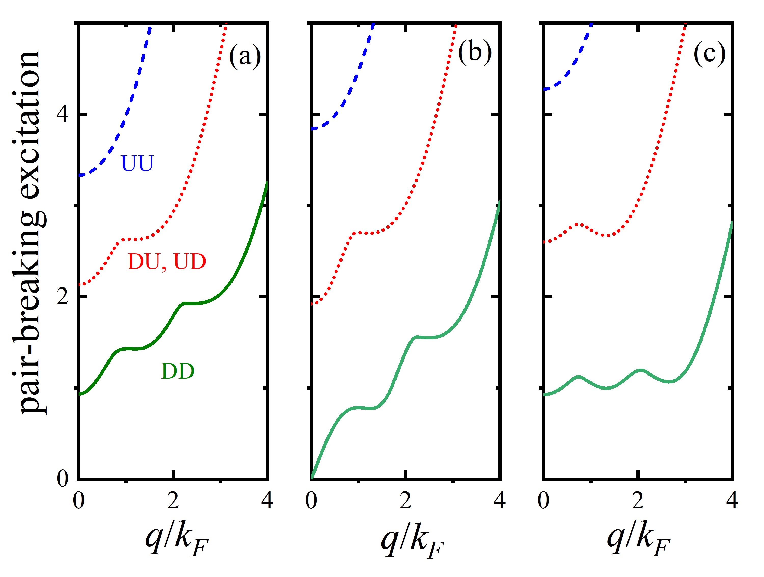
Figure 4: All kinds of threshold energy of pair-breaking excitation in different momenta at (a) $h=0.6E_{F}$, (b) $h=0.96E_{F}$ and (c) $h=1.3E_{F}$. Olive solid line: $D_{\textbf{{k}}}\leftrightarrow D_{\textbf{{k}}+\textbf{{q}}}.$ Red dotted line: $D_{\textbf{{k}}}\leftrightarrow U_{\textbf{{k}}+\textbf{{q}}}$ and $U_{\textbf{{k}}}\leftrightarrow D_{\textbf{{k}}+\textbf{{q}}}$. Blue dashed line: $U_{\textbf{{k}}}\leftrightarrow U_{\textbf{{k}}+\textbf{{q}}}$.

When the transferred energy $\omega$ is large enough, the excitation of the system is dominated by the sing-particle excitation. A pair-breaking of Cooper pairs will occur and make pairs be broken into free Fermi atoms. Indeed a great regime of the dynamical excitation in Fig. 2 is dominated by this pair-breaking effect. In the density dynamic structure factor $S_{n}$, this effect usually is very obvious in a relatively large transferred momentum $\textbf{{q}}>k_{F}$, where the collective excitation is strongly depressed. Different from the conventional Fermi superfluid, this single-particle excitation takes up a large regime in the spin dynamic structure factor $S_{s}$, even for a small or zero transferred momentum q. To understand this, it is necessary to study the threshold energy to break a Cooper pair. This pair-breaking excitation is related to two branches of quasi-particle spectra $U_{\textbf{{k}}}$ and $D_{\textbf{{k}}}$. The two atoms forming a Cooper-pair can come from the same or opposite branch of single particle spectrum. This two-branch spectrum structure generates four kinds of mechanism to break a Cooper pair, namely the $DD$, $DU$, $UD$, and $UU$ type. The minimum energy at a certain momentum q to break a pair is ${\rm min}[D_{\textbf{{k}}}+D_{\textbf{{k}}+\textbf{{q}}}]$, ${\rm min}[D_{\textbf{{k}}}+U_{\textbf{{k}}+\textbf{{q}}}]$, ${\rm min}[U_{\textbf{{k}}}+D_{\textbf{{k}}+\textbf{{q}}}]$ or ${\rm min}[U_{\textbf{{k}}}+U_{\textbf{{k}}+\textbf{{q}}}]$. Here the $DU$ and $UD$ excitations are overlapped with each other, and finally display three kinds of pair-breaking excitation regime. The minimum energy in these pair-breaking excitation are shown by three panels of Fig. 4, which are also displayed by the dotted lines in Fig. 2. The lowest olive line denotes the $DD$ type minimum energy (${\rm min}[D_{\textbf{{k}}}+D_{\textbf{{k}}+\textbf{{q}}}]$) to break a Cooper pair at a certain q, and atoms forming a Cooper pair are both from the down-branch quasi-particle spectrum $D_{\textbf{{k}}}$. Generally this value is always larger than zero in both BCS superfluid (panel (a)) and topological superfluid (panel (c)). However it will touch zero at the critical Zeeman field $h=0.96E_{F}$ (panel (b)), which is an important signal of this continuous phase transition. The red line denotes the minimum energy of cross-spectrum excitation ($DU$ and $UD$ type). The two atoms in a pair come from different branches of spectrum. This excitation starts from the ${\rm min}[D_{\textbf{{k}}}+U_{\textbf{{k}}+\textbf{{q}}}]$, and it requires an energy higher than the $DD$ one. This cross-spectrum excitation also reflects the coupling effect between spin- and orbital motion, and it is much easier to be observed in the spin dynamic structure factor than that in density one. The blue dashed line is the minimum energy in $UU$ excitation. Its energy is the largest among three kinds of pair-breaking excitation, however the excitation signal of $UU$ excitation is the weakest.

Besides all global minima discussed above, there are also some possible local minima in these pair-breaking excitations, which generate some edges in the dynamic structure factor. For example, some horizon edges emerge when $\omega$ is a little lower than $2E_{F}$ in the dynamic structure factor of Fig. 2, which is from the local minimum of the $DD$ type pair-breaking excitation.

To better understand the dynamical excitation in these colorful panels, we also discuss the dynamic structure factor at a fixed transferred momentum q.

III.2 Dynamic excitation at a constant momentum q

For a large transferred momentum $\textbf{{q}}\gg k_{F}$, the dynamic structure factor is dominated by the single-particle excitation. As shown in Fig. 5, we investigate the density and spin dynamic structure factors at $\textbf{{q}}=4k_{F}$ between BCS and topological superfluid. In all three panels, we always find a high excitation signal in density dynamic structure factor (gray solid lines) around $\omega=8E_{F}$. In fact it is the molecular Cooper-pair excitation, whose dispersion relation can be easily explained by $\varepsilon_{k}=\textbf{{q}}^{2}/2M$ and $M=2m$ is the mass a two-atom molecule. Also the single-atom excitation arrives its maximum around $\textbf{{q}}^{2}/2m\thickapprox 16E_{F}$ here. The olive and red arrows respectively mark the threshold energy to break a Cooper pair in $DD$ and $DU$ (or $UD$) type excitation. Different from the 3D crossover Fermi superfluid (Combescot2006m, ), the Rashba-SOC effect makes $DD$ pair-breaking excitation happen earlier than molecular excitation, no matter the value of Zeeman field $h$.

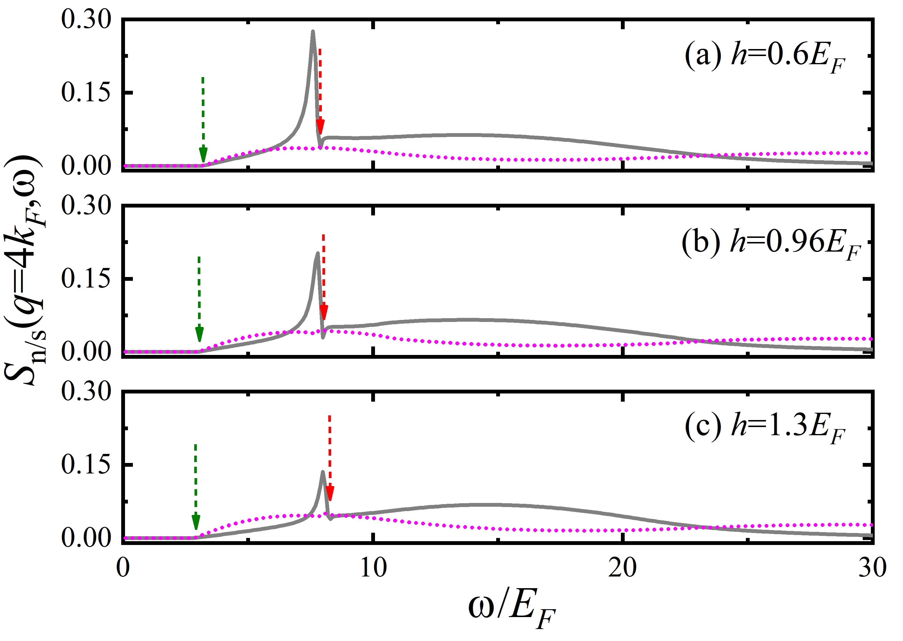
Figure 5: The density (gray) and spin (magenta) dynamical structure factor at transferred momentum $\textbf{{q}}=4k_{F}$. (a) $h=0.6E_{F}$ at BCS superfluid, (b) $h=0.96E_{F}$ at transition point, (c) $h=1.3E_{F}$ at topological superfluid.

When taking transferred momentum $\textbf{{q}}=2k_{F}$, the collective phonon has already merged into the regime of single-particle excitation. The dynamic structure factor is dominated by strong signals of pair-breaking excitation. As shown in Fig. 6, both curves of $S_{n}$ and $S_{s}$ have many twists which means they exhibit rich oscillations, and the two-olive arrows respectively mark the global (left) and local (right) minimum energy to break a Cooper pair according to $DD$ type excitation, and one red-dashed arrow marks the minimum energy of $DU$ (or $UD$) type excitation. In all three panels, small peaks (left side of red arrow) in density dynamic structure factor display the two-atom molecule excitation around $\omega=2.9E_{F}$, the obvious deviation from dispersion line $\varepsilon_{k}=\textbf{{q}}^{2}/2M=4E_{F}$ is due to its coupling effect to pair-breaking excitation in this relative weak transferred momentum ($\textbf{{q}}=2k_{F}$).

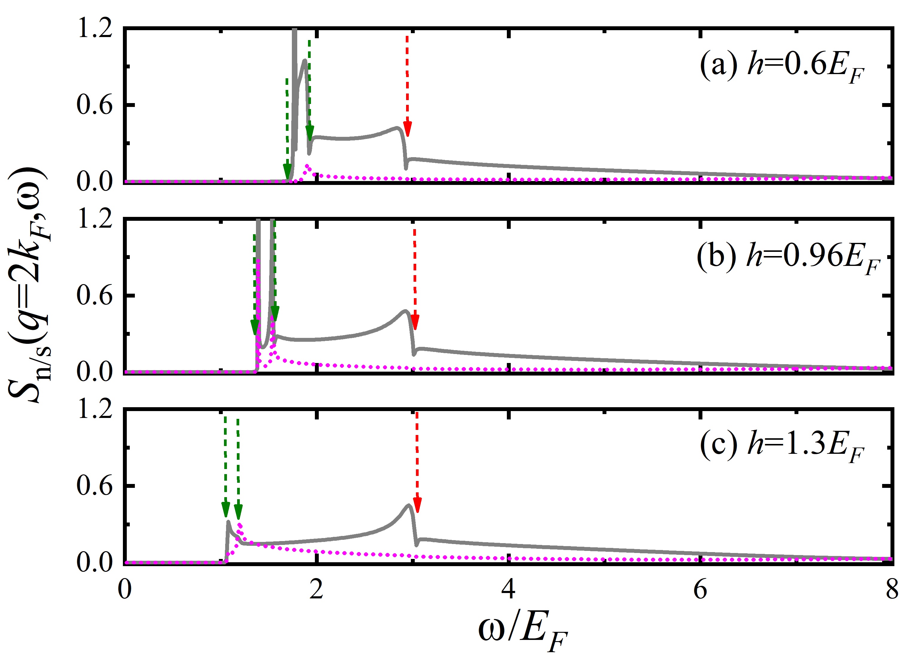
Figure 6: The density (gray) and spin (magenta) dynamical structure factor at transferred momentum $\textbf{{q}}=2k_{F}$. The arrangement of parameters in these three panels is the same as that in Fig. 5.

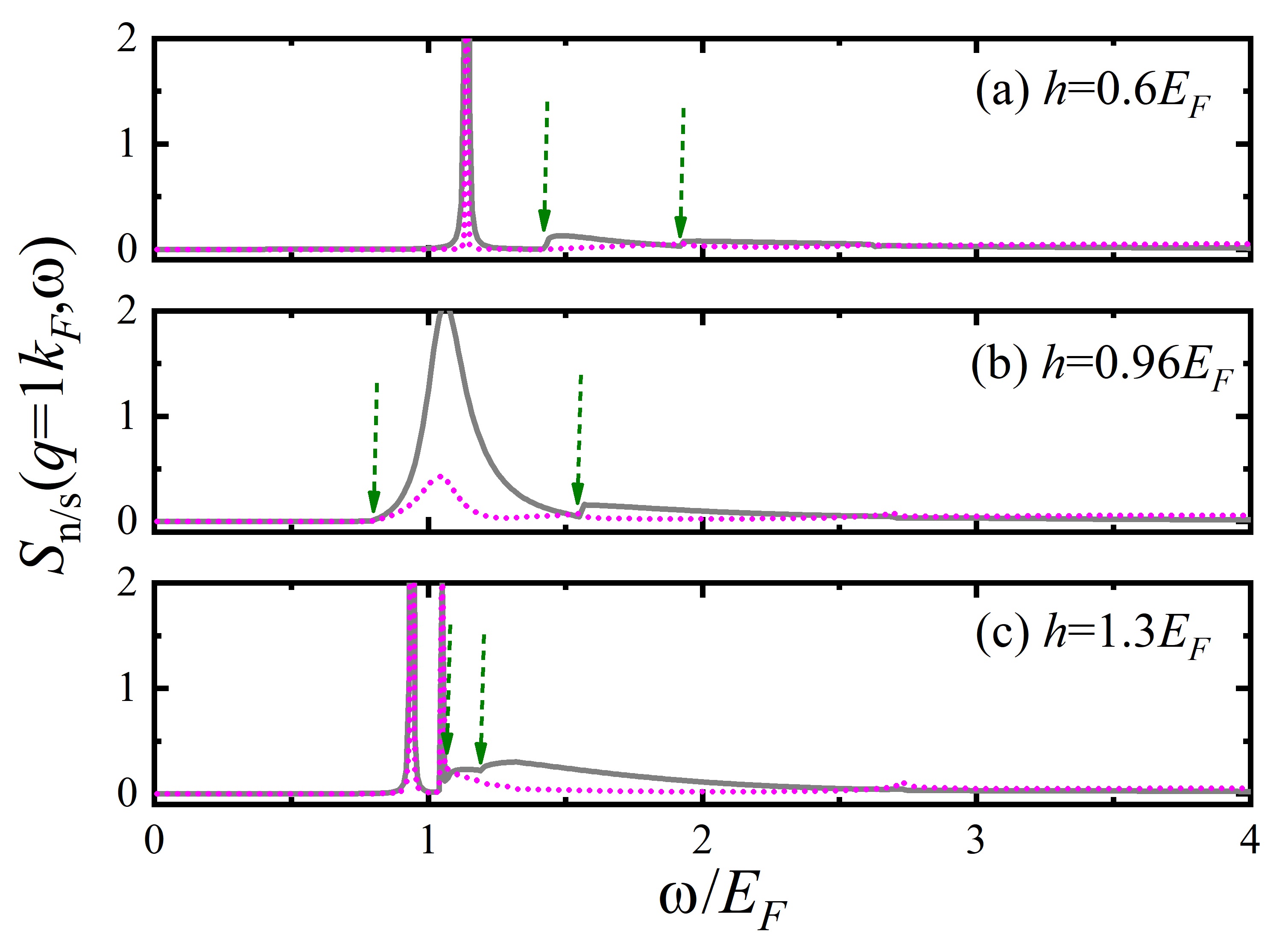
Figure 7: The density (gray) and spin (magenta) dynamical structure factor at transferred momentum $\textbf{{q}}=1k_{F}$. The arrangement of parameters in these three panels is the same as that in Fig. 5.

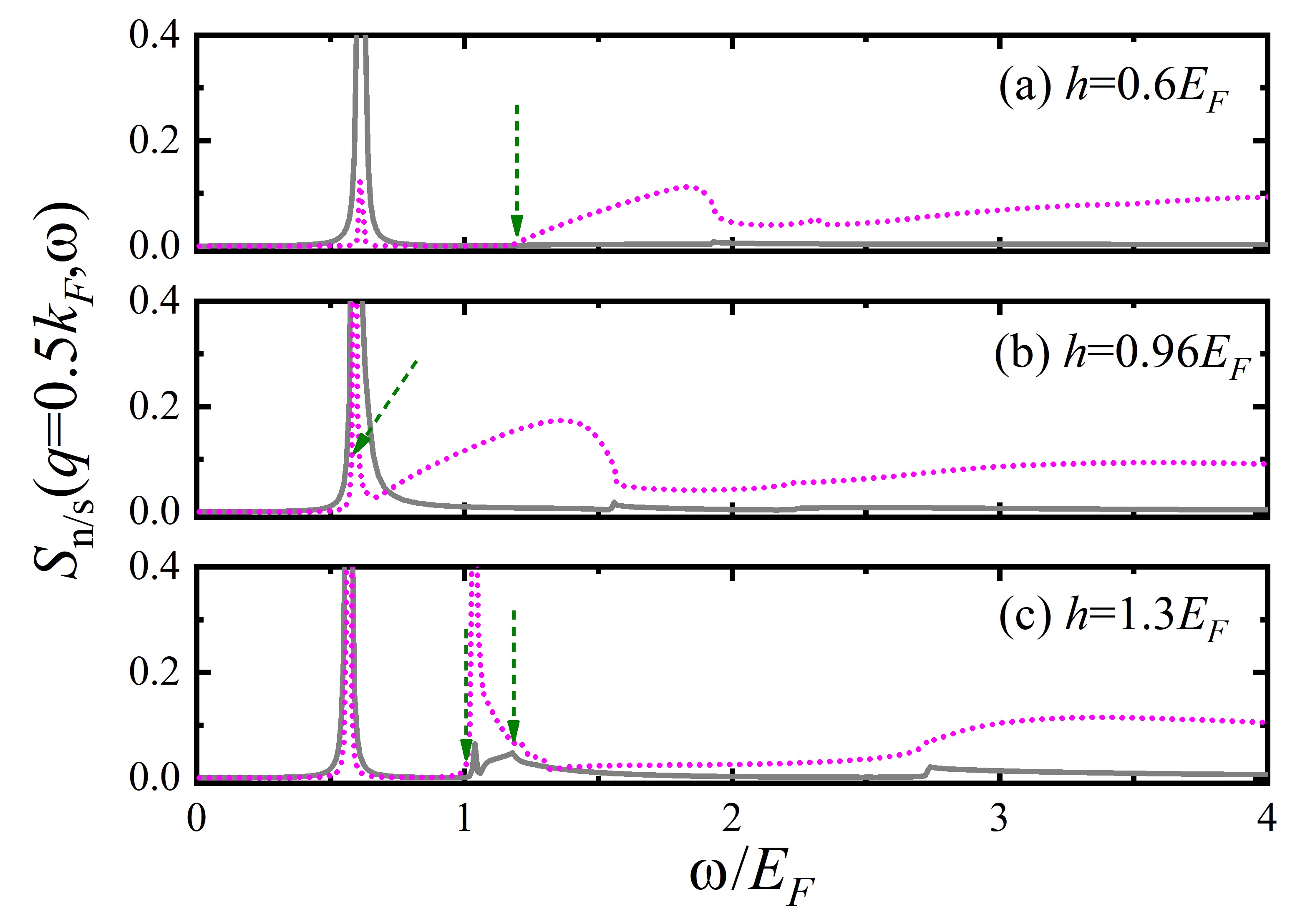
Figure 8: The density (gray) and spin (magenta) dynamical structure factor at transferred momentum $\textbf{{q}}=0.5k_{F}$. The arrangement of parameters in these three panels is the same as that in Fig. 5.

For a transferred momentum q at the order of Fermi wave vector $k_{F}$ (or smaller than $k_{F}$), the collective phonon excitation can be separated from the pair-breaking excitation, and happens at a smaller energy than pair-breaking effect. At the panel (a) and (c) of Fig. 7 and 8, strong sharp peaks are shown in the most left side of the dynamic structure factor, whose excitation energy are smaller than the global minimum energy of $DD$ type pair-breaking excitation. And the separation energy between phonon excitation and $DD$ type threshold excitation is relatively small in the topological superfluid ($h=1.3E_{F}$) since it has a weaker order parameter $\Delta$ than that in the BCS superfluid ($h=0.6E_{F}$). However in the point of phase transition $h=0.96E_{F}$ (shown by panel (b) of Figs. 7 and 8), the phonon excitation is just overlapped with the beginning of the gapless $DD$ type pair-breaking excitation, and give a finite width to the phonon peak at $\textbf{{q}}=1k_{F}$ (panel (b) of Fig. 7). At $\textbf{{q}}=0.5k_{F}$, although these two excitations are still mixed with each other at $h=0.96E_{F}$, this small transferred momentum q generates a relative weaker strength of $DD$ excitation. The phonon excitation is still very sharp in the density dynamic structure factor, and the spin dynamic structure factor can do help to track the signal of $DD$ excitation and display a bump structure closely following the phonon peak.

IV Conclusions and outlook

In summary, we numerically calculate the density and spin dynamic structure factor of 2D Rashba SOC Fermi superfluid with random phase approximation during a continuous phase transition between BCS and topological superfluids. The dynamic structure factor presents rich excitation signals, including collective phonon excitation, molecular or atomic excitations, and pair-breaking excitations. The gapless collective phonon excitation requires the smallest excitation energy in both BCS and topological superfluid. In the critical point of phase transition, the phonon excitation is overlapped with a gapless $DD$ type pair-breaking excitation, and also is imparted a finite expansion width to the phonon peak, which is a delta-like peak when far from critical point of phase transition. For a larger transferred momentum q, the strength of phonon excitation gradually decreases and merges into the pair-breaking excitation regime, and the excitation signals in both density and spin dynamic structure factor are dominated by single-particle excitation, including three kinds of pair-breaking excitation, two-atom molecular and single atomic excitations. The two-atom molecular (single atomic) excitations can be well explained by an ideal single molecule (atom) dispersion relation at a very large transferred momentum $\textbf{{q}}\gg k_{F}$. Our research about dynamic structure factor can do help to understand the dynamical excitation information in both BCS and topological matter state, distinguish different matter state during phase transition and judge the location of phase transition.

In the near future, it will be interesting to bring some non-uniform structures, like edge, impurity, or soliton (vortex), to this system, by which it is expected to investigate some excitations related to the generation of Majorana fermions (Majorana1937nc, ; Liu2013, ; Xu2014, ; Liu2015, ), which is absent in the current work. Experimentally the edge can be brought by a hard wall or a harmonic trap, and soliton can be generated by a phase-imprinting technique (KongPRA2021, ). So it will be worth to carry out calculation to these non-uniform systems.

V Acknowledgements

This research was supported by the National Natural Science Foundation of China, Grants No. 11804177 (P.Z.), No. 11547034 (H.Z.), No. 11974384 (S.-G.P.); NKRDP under Grant No. 2016YFA0301503 (S.-G.P.).

VI Appendix

The exact diagonalization of mean-field Hamiltonian $H_{{\rm mf}}$ is carried out by motion equation of Green’s function $\omega\left\langle\left\langle c_{1}|c_{2}\right\rangle\right\rangle=\left\langle\left[c_{1},c_{2}\right]_{+}\right\rangle+\left\langle\left\langle\left[c_{1},H_{{\rm mf}}\right]|c_{2}\right\rangle\right\rangle$, where $c_{1}$ and $c_{2}$ are any possible fermionic operators of the system, and the double-bracket notation $\left\langle\left\langle c_{1}|c_{2}\right\rangle\right\rangle$ is the corresponding momentum-energy Fourier transformation of space-time Green’s function $G(r_{1},\tau,r_{2},0)=-\left<T\psi_{1}(r_{1},\tau)\psi_{2}(r_{2},0)\right>$. Finally we find that the system has six independent Green’s functions. In this appendix, we will list expressions of six independent Green’s functions and mean-field response function $\chi^{0}=A+B$. The six independent Green’s functions are $G_{1}\left(\textbf{{k}},\omega\right)=\sum_{l}\left[G_{1}\right]_{\textbf{{k}}}^{l}/\left(\omega-E_{\textbf{{k}}}^{l}\right)$ with

$$\begin{array}[]{cl}\left[G_{1}\right]_{\textbf{{k}}}^{(1)}&=\frac{U_{\textbf{{k}}}^{2}-\left(h^{2}+\textbf{{k}}^{2}\lambda^{2}+E_{\textbf{{k}}}^{2}+2h\xi_{\textbf{{k}}}\right)}{2\left(U_{\textbf{{k}}}^{2}-D_{\textbf{{k}}}^{2}\right)}\\ &+\frac{\left(\xi_{\textbf{{k}}}-h\right)U_{\textbf{{k}}}^{2}-\left(\xi_{\textbf{{k}}}+h\right)\left(E_{\textbf{{k}}}^{2}-h^{2}-\textbf{{k}}^{2}\lambda^{2}\right)}{2U_{\textbf{{k}}}\left(U_{\textbf{{k}}}^{2}-D_{\textbf{{k}}}^{2}\right)},\end{array}$$

$$\begin{array}[]{cl}\left[G_{1}\right]_{\textbf{{k}}}^{(-1)}&=\frac{U_{\textbf{{k}}}^{2}-\left(h^{2}+\textbf{{k}}^{2}\lambda^{2}+E_{\textbf{{k}}}^{2}+2h\xi_{\textbf{{k}}}\right)}{2\left(U_{\textbf{{k}}}^{2}-D_{\textbf{{k}}}^{2}\right)}\\ &-\frac{\left(\xi_{\textbf{{k}}}-h\right)U_{\textbf{{k}}}^{2}-\left(\xi_{\textbf{{k}}}+h\right)\left(E_{\textbf{{k}}}^{2}-h^{2}-\textbf{{k}}^{2}\lambda^{2}\right)}{2U_{\textbf{{k}}}\left(U_{\textbf{{k}}}^{2}-D_{\textbf{{k}}}^{2}\right)},\end{array}$$

$$\begin{array}[]{cl}\left[G_{1}\right]_{\textbf{{k}}}^{(2)}&=-\frac{D_{\textbf{{k}}}^{2}-\left(h^{2}+\textbf{{k}}^{2}\lambda^{2}+E_{\textbf{{k}}}^{2}+2h\xi_{\textbf{{k}}}\right)}{2\left(U_{\textbf{{k}}}^{2}-D_{\textbf{{k}}}^{2}\right)}\\ &-\frac{\left(\xi_{\textbf{{k}}}-h\right)D_{\textbf{{k}}}^{2}-\left(\xi_{\textbf{{k}}}+h\right)\left(E_{\textbf{{k}}}^{2}-h^{2}-\textbf{{k}}^{2}\lambda^{2}\right)}{2D_{\textbf{{k}}}\left(U_{\textbf{{k}}}^{2}-D_{\textbf{{k}}}^{2}\right)},\end{array}$$

$$\begin{array}[]{cl}\left[G_{1}\right]_{\textbf{{k}}}^{(-2)}&=-\frac{D_{\textbf{{k}}}^{2}-\left(h^{2}+\textbf{{k}}^{2}\lambda^{2}+E_{\textbf{{k}}}^{2}+2h\xi_{\textbf{{k}}}\right)}{2\left(U_{\textbf{{k}}}^{2}-D_{\textbf{{k}}}^{2}\right)}\\ &+\frac{\left(\xi_{\textbf{{k}}}-h\right)D_{\textbf{{k}}}^{2}-\left(\xi_{\textbf{{k}}}+h\right)\left(E_{\textbf{{k}}}^{2}-h^{2}-\textbf{{k}}^{2}\lambda^{2}\right)}{2D_{\textbf{{k}}}\left(U_{\textbf{{k}}}^{2}-D_{k}^{2}\right)}.\end{array}$$

$G_{2}\left(\textbf{{k}},\omega\right)=\sum_{l}\left[G_{2}\right]_{\textbf{{k}}}^{l}/\left(\omega-E_{\textbf{{k}}}^{l}\right)$ with

$$\begin{array}[]{cl}\left[G_{2}\right]_{\textbf{{k}}}^{(1)}&=\frac{U_{\textbf{{k}}}^{2}-\left(h^{2}+\textbf{{k}}^{2}\lambda^{2}+E_{\textbf{{k}}}^{2}-2h\xi_{\textbf{{k}}}\right)}{2\left(U_{\textbf{{k}}}^{2}-D_{\textbf{{k}}}^{2}\right)}\\ &+\frac{\left(\xi_{\textbf{{k}}}+h\right)U_{\textbf{{k}}}^{2}-\left(\xi_{\textbf{{k}}}-h\right)\left(E_{\textbf{{k}}}^{2}-h^{2}-\textbf{{k}}^{2}\lambda^{2}\right)}{2U_{\textbf{{k}}}\left(U_{\textbf{{k}}}^{2}-D_{\textbf{{k}}}^{2}\right)},\end{array}$$

$$\begin{array}[]{cl}\left[G_{2}\right]_{\textbf{{k}}}^{(-1)}&=\frac{U_{\textbf{{k}}}^{2}-\left(h^{2}+\textbf{{k}}^{2}\lambda^{2}+E_{\textbf{{k}}}^{2}-2h\xi_{\textbf{{k}}}\right)}{2\left(U_{\textbf{{k}}}^{2}-D_{\textbf{{k}}}^{2}\right)}\\ &-\frac{\left(\xi_{\textbf{{k}}}+h\right)U_{\textbf{{k}}}^{2}-\left(\xi_{\textbf{{k}}}-h\right)\left(E_{\textbf{{k}}}^{2}-h^{2}-\textbf{{k}}^{2}\lambda^{2}\right)}{2U_{\textbf{{k}}}\left(U_{\textbf{{k}}}^{2}-D_{\textbf{{k}}}^{2}\right)},\end{array}$$

$$\begin{array}[]{cl}\left[G_{2}\right]_{\textbf{{k}}}^{(2)}&=-\frac{D_{\textbf{{k}}}^{2}-\left(h^{2}+\textbf{{k}}^{2}\lambda^{2}+E_{\textbf{{k}}}^{2}-2h\xi_{\textbf{{k}}}\right)}{2\left(U_{\textbf{{k}}}^{2}-D_{\textbf{{k}}}^{2}\right)}\\ &-\frac{\left(\xi_{\textbf{{k}}}+h\right)D_{\textbf{{k}}}^{2}-\left(\xi_{\textbf{{k}}}-h\right)\left(E_{\textbf{{k}}}^{2}-h^{2}-\textbf{{k}}^{2}\lambda^{2}\right)}{2D_{\textbf{{k}}}\left(U_{\textbf{{k}}}^{2}-D_{\textbf{{k}}}^{2}\right)},\end{array}$$

$$\begin{array}[]{cl}\left[G_{2}\right]_{\textbf{{k}}}^{(-2)}&=-\frac{D_{\textbf{{k}}}^{2}-\left(h^{2}+\textbf{{k}}^{2}\lambda^{2}+E_{\textbf{{k}}}^{2}-2h\xi_{\textbf{{k}}}\right)}{2\left(U_{\textbf{{k}}}^{2}-D_{\textbf{{k}}}^{2}\right)}\\ &+\frac{\left(\xi_{\textbf{{k}}}+h\right)D_{\textbf{{k}}}^{2}-\left(\xi_{\textbf{{k}}}-h\right)\left(E_{\textbf{{k}}}^{2}-h^{2}-\textbf{{k}}^{2}\lambda^{2}\right)}{2D_{\textbf{{k}}}\left(U_{\textbf{{k}}}^{2}-D_{\textbf{{k}}}^{2}\right)},\end{array}$$

$\varGamma\left(\textbf{{k}},\omega\right)=\sum_{l}\left[\varGamma\right]_{\textbf{{k}}}^{l}/\left(\omega-E_{\textbf{{k}}}^{l}\right)$ with

$$\begin{array}[]{l}\left[\varGamma\right]_{\textbf{{k}}}^{(1)}=+\frac{\Delta h}{U_{\textbf{{k}}}^{2}-D_{\textbf{{k}}}^{2}}-\frac{\Delta\left[U_{\textbf{{k}}}^{2}+\left(h^{2}-\textbf{{k}}^{2}\lambda^{2}-E_{\textbf{{k}}}^{2}\right)\right]}{2U_{\textbf{{k}}}\left(U_{\textbf{{k}}}^{2}-D_{\textbf{{k}}}^{2}\right)},\\ \left[\varGamma\right]_{\textbf{{k}}}^{(-1)}=+\frac{\Delta h}{U_{\textbf{{k}}}^{2}-D_{\textbf{{k}}}^{2}}+\frac{\Delta\left[U_{\textbf{{k}}}^{2}+\left(h^{2}-\textbf{{k}}^{2}\lambda^{2}-E_{\textbf{{k}}}^{2}\right)\right]}{2U_{\textbf{{k}}}\left(U_{\textbf{{k}}}^{2}-D_{\textbf{{k}}}^{2}\right)},\\ \left[\varGamma\right]_{\textbf{{k}}}^{(2)}=-\frac{\Delta h}{U_{\textbf{{k}}}^{2}-D_{\textbf{{k}}}^{2}}+\frac{\Delta\left[D_{\textbf{{k}}}^{2}+\left(h^{2}-\textbf{{k}}^{2}\lambda^{2}-E_{\textbf{{k}}}^{2}\right)\right]}{2D_{\textbf{{k}}}\left(U_{\textbf{{k}}}^{2}-D_{\textbf{{k}}}^{2}\right)},\\ \left[\varGamma\right]_{\textbf{{k}}}^{(-2)}=-\frac{\Delta h}{U_{\textbf{{k}}}^{2}-D_{\textbf{{k}}}^{2}}-\frac{\Delta\left[D_{\textbf{{k}}}^{2}+\left(h^{2}-\textbf{{k}}^{2}\lambda^{2}-E_{\textbf{{k}}}^{2}\right)\right]}{2D_{\textbf{{k}}}\left(U_{\textbf{{k}}}^{2}-D_{\textbf{{k}}}^{2}\right)}.\end{array}$$

$S\left(\textbf{{k}},\omega\right)=\sum_{l}\left[S\right]_{\textbf{{k}}}^{l}/\left(\omega-E_{\textbf{{k}}}^{l}\right)$ with

$$\begin{array}[]{l}\left[S\right]_{\textbf{{k}}}^{(1)}=\left(k_{y}-ik_{x}\right)\lambda\left[+\frac{\xi_{\textbf{{k}}}}{U_{\textbf{{k}}}^{2}-D_{\textbf{{k}}}^{2}}+\frac{U_{\textbf{{k}}}^{2}+\left(\xi_{\textbf{{k}}}^{2}-h^{2}-\textbf{{k}}^{2}\lambda^{2}-\Delta^{2}\right)}{2U_{\textbf{{k}}}\left(U_{\textbf{{k}}}^{2}-D_{\textbf{{k}}}^{2}\right)}\right],\\ \left[S\right]_{\textbf{{k}}}^{(-1)}=\left(k_{y}-ik_{x}\right)\lambda\left[+\frac{\xi_{\textbf{{k}}}}{U_{\textbf{{k}}}^{2}-D_{\textbf{{k}}}^{2}}-\frac{U_{\textbf{{k}}}^{2}+\left(\xi_{\textbf{{k}}}^{2}-h^{2}-\textbf{{k}}^{2}\lambda^{2}-\Delta^{2}\right)}{2U_{\textbf{{k}}}\left(U_{\textbf{{k}}}^{2}-D_{\textbf{{k}}}^{2}\right)}\right],\\ \left[S\right]_{\textbf{{k}}}^{(2)}=\left(k_{y}-ik_{x}\right)\lambda\left[-\frac{\xi_{\textbf{{k}}}}{U_{\textbf{{k}}}^{2}-D_{\textbf{{k}}}^{2}}-\frac{D_{\textbf{{k}}}^{2}+\left(\xi_{\textbf{{k}}}^{2}-h^{2}-\textbf{{k}}^{2}\lambda^{2}-\Delta^{2}\right)}{2D_{\textbf{{k}}}\left(U_{\textbf{{k}}}^{2}-D_{\textbf{{k}}}^{2}\right)}\right],\\ \left[S\right]_{\textbf{{k}}}^{(-2)}=\left(k_{y}-ik_{x}\right)\lambda\left[-\frac{\xi_{\textbf{{k}}}}{U_{\textbf{{k}}}^{2}-D_{\textbf{{k}}}^{2}}+\frac{D_{\textbf{{k}}}^{2}+\left(\xi_{\textbf{{k}}}^{2}-h^{2}-\textbf{{k}}^{2}\lambda^{2}-\Delta^{2}\right)}{2D_{\textbf{{k}}}\left(U_{\textbf{{k}}}^{2}-D_{\textbf{{k}}}^{2}\right)}\right].\end{array}$$

$F_{1}\left(\textbf{{k}},\omega\right)=\sum_{l}\left[F_{1}\right]_{\textbf{{k}}}^{l}/\left(\omega-E_{\textbf{{k}}}^{l}\right)$ with

$$\begin{array}[]{c}\left[F_{1}\right]_{\textbf{{k}}}^{(1)}=-\left[F_{1}\right]_{\textbf{{k}}}^{(-1)}=+\frac{\Delta\lambda\left(k_{y}+ik_{x}\right)\left(\xi_{\textbf{{k}}}+h\right)}{U_{\textbf{{k}}}\left(U_{\textbf{{k}}}^{2}-D_{\textbf{{k}}}^{2}\right)},\\ \left[F_{1}\right]_{\textbf{{k}}}^{(2)}=-\left[F_{1}\right]_{\textbf{{k}}}^{(-2)}=-\frac{\Delta\lambda\left(k_{y}+ik_{x}\right)\left(\xi_{\textbf{{k}}}+h\right)}{D_{\textbf{{k}}}\left(U_{\textbf{{k}}}^{2}-D_{\textbf{{k}}}^{2}\right)}.\end{array}$$

$F_{2}\left(\textbf{{k}},\omega\right)=\sum_{l}\left[F_{2}\right]_{\textbf{{k}}}^{l}/\left(\omega-E_{\textbf{{k}}}^{l}\right)$ with

$$\begin{array}[]{c}\left[F_{2}\right]_{\textbf{{k}}}^{(1)}=-\left[F_{2}\right]_{\textbf{{k}}}^{(-1)}=-\frac{\Delta\lambda\left(k_{y}-ik_{x}\right)\left(\xi_{\textbf{{k}}}-h\right)}{U_{\textbf{{k}}}\left(U_{\textbf{{k}}}^{2}-D_{\textbf{{k}}}^{2}\right)},\\ \left[F_{2}\right]_{\textbf{{k}}}^{(2)}=-\left[F_{2}\right]_{\textbf{{k}}}^{(-2)}=+\frac{\Delta\lambda\left(k_{y}-ik_{x}\right)\left(\xi_{\textbf{{k}}}-h\right)}{D_{\textbf{{k}}}\left(U_{\textbf{{k}}}^{2}-D_{\textbf{{k}}}^{2}\right)}.\end{array}$$

The expressions of all 9 independent matrix elements in mean-field response function $A$ are

$A_{11}=+\underset{\textbf{{p}}ll^{\prime}}{\sum}\left[G_{1}\right]_{\textbf{{p}}}^{l}\left[G_{1}\right]_{\textbf{{p}}+\textbf{{q}}}^{l^{\prime}}\frac{f\left(E_{\textbf{{p}}}^{l}\right)-f\left(E_{\textbf{{p}}+\textbf{{q}}}^{l^{\prime}}\right)}{i\omega_{n}+E_{\textbf{{p}}}^{l}-E_{\textbf{{p}}+\textbf{{q}}}^{l^{\prime}}},$

$A_{12}=-\underset{\textbf{{p}}ll^{\prime}}{\sum}\left[\varGamma\right]_{\textbf{{p}}}^{l}\left[\varGamma\right]_{\textbf{{p}}+\textbf{{q}}}^{l^{\prime}}\frac{f\left(E_{\textbf{{p}}}^{l}\right)-f\left(E_{\textbf{{p}}+\textbf{{q}}}^{l^{\prime}}\right)}{i\omega_{n}+E_{\textbf{{p}}}^{l}-E_{\textbf{{p}}+\textbf{{q}}}^{l^{\prime}}},$

$A_{13}=+\underset{\textbf{{p}}ll^{\prime}}{\sum}\left[G_{1}\right]_{\textbf{{p}}}^{l}\left[\varGamma\right]_{\textbf{{p}}+\textbf{{q}}}^{l^{\prime}}\frac{f\left(E_{\textbf{{p}}}^{l}\right)-f\left(E_{\textbf{{p}}+\textbf{{q}}}^{l^{\prime}}\right)}{i\omega_{n}+E_{\textbf{{p}}}^{l}-E_{\textbf{{p}}+\textbf{{q}}}^{l^{\prime}}},$

$A_{14}=+\underset{\textbf{{p}}ll^{\prime}}{\sum}\left[\varGamma\right]_{\textbf{{p}}}^{l}\left[G_{1}\right]_{\textbf{{p}}+\textbf{{q}}}^{l^{\prime}}\frac{f\left(E_{\textbf{{p}}}^{l}\right)-f\left(E_{\textbf{{p}}+\textbf{{q}}}^{l^{\prime}}\right)}{i\omega_{n}+E_{\textbf{{p}}}^{l}-E_{\textbf{{p}}+\textbf{{q}}}^{l^{\prime}}},$

$A_{22}=+\underset{\textbf{{p}}ll^{\prime}}{\sum}\left[G_{2}\right]_{\textbf{{p}}}^{l}\left[G_{2}\right]_{\textbf{{p}}+\textbf{{q}}}^{l^{\prime}}\frac{f\left(E_{\textbf{{p}}}^{l}\right)-f\left(E_{\textbf{{p}}+\textbf{{q}}}^{l^{\prime}}\right)}{i\omega_{n}+E_{\textbf{{p}}}^{l}-E_{\textbf{{p}}+\textbf{{q}}}^{l^{\prime}}},$

$A_{23}=-\underset{\textbf{{p}}ll^{\prime}}{\sum}\left[G_{2}\right]_{\textbf{{p}}}^{l}\left[\varGamma\right]_{\textbf{{p}}+\textbf{{q}}}^{-l^{\prime}}\frac{f\left(E_{\textbf{{p}}}^{l}\right)-f\left(E_{\textbf{{p}}+\textbf{{q}}}^{l^{\prime}}\right)}{i\omega_{n}+E_{\textbf{{p}}}^{l}-E_{\textbf{{p}}+\textbf{{q}}}^{l^{\prime}}},$

$A_{24}=-\underset{\textbf{{p}}ll^{\prime}}{\sum}\left[\varGamma\right]_{\textbf{{p}}}^{-l}\left[G_{2}\right]_{\textbf{{p}}+\textbf{{q}}}^{l^{\prime}}\frac{f\left(E_{\textbf{{p}}}^{l}\right)-f\left(E_{\textbf{{p}}+\textbf{{q}}}^{l^{\prime}}\right)}{i\omega_{n}+E_{\textbf{{p}}}^{l}-E_{\textbf{{p}}+\textbf{{q}}}^{l^{\prime}}},$

$A_{34}=+\underset{\textbf{{p}}ll^{\prime}}{\sum}\left[G_{2}\right]_{\textbf{{p}}}^{-l}\left[G_{1}\right]_{\textbf{{p}}+\textbf{{q}}}^{l^{\prime}}\frac{f\left(E_{\textbf{{p}}}^{l}\right)-f\left(E_{\textbf{{p}}+\textbf{{q}}}^{l^{\prime}}\right)}{i\omega_{n}+E_{\textbf{{p}}}^{l}-E_{\textbf{{p}}+\textbf{{q}}}^{l^{\prime}}},$

$A_{43}=+\underset{\textbf{{p}}ll^{\prime}}{\sum}\left[G_{1}\right]_{\textbf{{p}}}^{l}\left[G_{2}\right]_{\textbf{{p}}+\textbf{{q}}}^{-l^{\prime}}\frac{f\left(E_{\textbf{{p}}}^{l}\right)-f\left(E_{\textbf{{p}}+\textbf{{q}}}^{l^{\prime}}\right)}{i\omega_{n}+E_{\textbf{{p}}}^{l}-E_{\textbf{{p}}+\textbf{{q}}}^{l^{\prime}}},$ where $f\left(x\right)=1/\left(e^{x/T}+1\right)$ is the Fermi-Dirac distribution function. The expressions of 16 independent matrix elements in mean-field response function $B$ are

$B_{11}=-\underset{\textbf{{p}}ll^{\prime}}{\sum}\left[F_{1}^{*}\right]_{\textbf{{p}}}^{l}\left[F_{1}\right]_{\textbf{{p}}+\textbf{{q}}}^{l^{\prime}}\frac{f\left(E_{\textbf{{p}}}^{l}\right)-f\left(E_{\textbf{{p}}+\textbf{{q}}}^{l^{\prime}}\right)}{i\omega_{n}+E_{\textbf{{p}}}^{l}-E_{\textbf{{p}}+\textbf{{q}}}^{l^{\prime}}},$

$B_{12}=+\underset{\textbf{{p}}ll^{\prime}}{\sum}\left[S\right]_{\textbf{{p}}}^{l}\left[S^{*}\right]_{\textbf{{p}}+\textbf{{q}}}^{l^{\prime}}\frac{f\left(E_{\textbf{{p}}}^{l}\right)-f\left(E_{\textbf{{p}}+\textbf{{q}}}^{l^{\prime}}\right)}{i\omega_{n}+E_{\textbf{{p}}}^{l}-E_{\textbf{{p}}+\textbf{{q}}}^{l^{\prime}}},$

$B_{13}=-\underset{\textbf{{p}}ll^{\prime}}{\sum}\left[S\right]_{\textbf{{p}}}^{l}\left[F_{1}\right]_{\textbf{{p}}+\textbf{{q}}}^{l^{\prime}}\frac{f\left(E_{\textbf{{p}}}^{l}\right)-f\left(E_{\textbf{{p}}+\textbf{{q}}}^{l^{\prime}}\right)}{i\omega_{n}+E_{\textbf{{p}}}^{l}-E_{\textbf{{p}}+\textbf{{q}}}^{l^{\prime}}},$

$B_{14}=-\underset{\textbf{{p}}ll^{\prime}}{\sum}\left[F_{1}^{*}\right]_{\textbf{{p}}}^{l}\left[S^{*}\right]_{\textbf{{p}}+\textbf{{q}}}^{l^{\prime}}\frac{f\left(E_{\textbf{{p}}}^{l}\right)-f\left(E_{\textbf{{p}}+\textbf{{q}}}^{l^{\prime}}\right)}{i\omega_{n}+E_{\textbf{{p}}}^{l}-E_{\textbf{{p}}+\textbf{{q}}}^{l^{\prime}}},$

$B_{21}=+\underset{\textbf{{p}}ll^{\prime}}{\sum}\left[S^{*}\right]_{\textbf{{p}}}^{l}\left[S\right]_{\textbf{{p}}+\textbf{{q}}}^{l^{\prime}}\frac{f\left(E_{\textbf{{p}}}^{l}\right)-f\left(E_{\textbf{{p}}+\textbf{{q}}}^{l^{\prime}}\right)}{i\omega_{n}+E_{\textbf{{p}}}^{l}-E_{\textbf{{p}}+\textbf{{q}}}^{l^{\prime}}},$

$B_{22}=-\underset{\textbf{{p}}ll^{\prime}}{\sum}\left[F_{2}\right]_{\textbf{{p}}}^{l}\left[F_{2}^{*}\right]_{\textbf{{p}}+\textbf{{q}}}^{l^{\prime}}\frac{f\left(E_{\textbf{{p}}}^{l}\right)-f\left(E_{\textbf{{p}}+\textbf{{q}}}^{l^{\prime}}\right)}{i\omega_{n}+E_{\textbf{{p}}}^{l}-E_{\textbf{{p}}+\textbf{{q}}}^{l^{\prime}}},$

$B_{23}=+\underset{\textbf{{p}}ll^{\prime}}{\sum}\left[S^{*}\right]_{\textbf{{p}}}^{l}\left[F_{2}\right]_{\textbf{{p}}+\textbf{{q}}}^{l^{\prime}}\frac{f\left(E_{\textbf{{p}}}^{l}\right)-f\left(E_{\textbf{{p}}+\textbf{{q}}}^{l^{\prime}}\right)}{i\omega_{n}+E_{\textbf{{p}}}^{l}-E_{\textbf{{p}}+\textbf{{q}}}^{l^{\prime}}},$

$B_{24}=+\underset{\textbf{{p}}ll^{\prime}}{\sum}\left[F_{2}^{*}\right]_{\textbf{{p}}}^{l}\left[S\right]_{\textbf{{p}}+\textbf{{q}}}^{l^{\prime}}\frac{f\left(E_{\textbf{{p}}}^{l}\right)-f\left(E_{\textbf{{p}}+\textbf{{q}}}^{l^{\prime}}\right)}{i\omega_{n}+E_{\textbf{{p}}}^{l}-E_{\textbf{{p}}+\textbf{{q}}}^{l^{\prime}}},$

$B_{31}=-\underset{\textbf{{p}}ll^{\prime}}{\sum}\left[F_{1}\right]_{\textbf{{p}}}^{l}\left[S\right]_{\textbf{{p}}+\textbf{{q}}}^{l^{\prime}}\frac{f\left(E_{\textbf{{p}}}^{l}\right)-f\left(E_{\textbf{{p}}+\textbf{{q}}}^{l^{\prime}}\right)}{i\omega_{n}+E_{\textbf{{p}}}^{l}-E_{\textbf{{p}}+\textbf{{q}}}^{l^{\prime}}},$

$B_{32}=+\underset{\textbf{{p}}ll^{\prime}}{\sum}\left[F_{2}\right]_{\textbf{{p}}}^{l}\left[S^{*}\right]_{\textbf{{p}}+\textbf{{q}}}^{l^{\prime}}\frac{f\left(E_{\textbf{{p}}}^{l}\right)-f\left(E_{\textbf{{p}}+\textbf{{q}}}^{l^{\prime}}\right)}{i\omega_{n}+E_{\textbf{{p}}}^{l}-E_{\textbf{{p}}+\textbf{{q}}}^{l^{\prime}}},$

$B_{33}=-\underset{\textbf{{p}}ll^{\prime}}{\sum}\left[F_{2}\right]_{\textbf{{p}}}^{l}\left[F_{1}\right]_{\textbf{{p}}+\textbf{{q}}}^{l^{\prime}}\frac{f\left(E_{\textbf{{p}}}^{l}\right)-f\left(E_{\textbf{{p}}+\textbf{{q}}}^{l^{\prime}}\right)}{i\omega_{n}+E_{\textbf{{p}}}^{l}-E_{\textbf{{p}}+\textbf{{q}}}^{l^{\prime}}},$

$B_{34}=+\underset{\textbf{{p}}ll^{\prime}}{\sum}\left[S\right]_{\textbf{{p}}}^{-l}\left[S^{*}\right]_{\textbf{{p}}+\textbf{{q}}}^{l^{\prime}}\frac{f\left(E_{\textbf{{p}}}^{l}\right)-f\left(E_{\textbf{{p}}+\textbf{{q}}}^{l^{\prime}}\right)}{i\omega_{n}+E_{\textbf{{p}}}^{l}-E_{\textbf{{p}}+\textbf{{q}}}^{l^{\prime}}},$

$B_{41}=-\underset{\textbf{{p}}ll^{\prime}}{\sum}\left[S^{*}\right]_{\textbf{{p}}}^{l}\left[F_{1}^{*}\right]_{\textbf{{p}}+\textbf{{q}}}^{l^{\prime}}\frac{f\left(E_{\textbf{{p}}}^{l}\right)-f\left(E_{\textbf{{p}}+\textbf{{q}}}^{l^{\prime}}\right)}{i\omega_{n}+E_{\textbf{{p}}}^{l}-E_{\textbf{{p}}+\textbf{{q}}}^{l^{\prime}}}.$

$B_{42}=+\underset{\textbf{{p}}ll^{\prime}}{\sum}\left[S\right]_{\textbf{{p}}}^{l}\left[F_{2}^{*}\right]_{\textbf{{p}}+\textbf{{q}}}^{l^{\prime}}\frac{f\left(E_{\textbf{{p}}}^{l}\right)-f\left(E_{\textbf{{p}}+\textbf{{q}}}^{l^{\prime}}\right)}{i\omega_{n}+E_{\textbf{{p}}}^{l}-E_{\textbf{{p}}+\textbf{{q}}}^{l^{\prime}}}.$

$B_{43}=+\underset{\textbf{{p}}ll^{\prime}}{\sum}\left[S\right]_{\textbf{{p}}}^{l}\left[S^{*}\right]_{\textbf{{p}}+\textbf{{q}}}^{-l^{\prime}}\frac{f\left(E_{\textbf{{p}}}^{l}\right)-f\left(E_{\textbf{{p}}+\textbf{{q}}}^{l^{\prime}}\right)}{i\omega_{n}+E_{\textbf{{p}}}^{l}-E_{\textbf{{p}}+\textbf{{q}}}^{l^{\prime}}}.$

$B_{44}=-\underset{\textbf{{p}}ll^{\prime}}{\sum}\left[F_{1}^{*}\right]_{\textbf{{p}}}^{l}\left[F_{2}^{*}\right]_{\textbf{{p}}+\textbf{{q}}}^{l^{\prime}}\frac{f\left(E_{\textbf{{p}}}^{l}\right)-f\left(E_{\textbf{{p}}+\textbf{{q}}}^{l^{\prime}}\right)}{i\omega_{n}+E_{\textbf{{p}}}^{l}-E_{\textbf{{p}}+\textbf{{q}}}^{l^{\prime}}}.$

References

- (1) I. Bloch, J. Dalibard, and W. Zwerger, Many-body physics with ultracold gases, Rev. Mod. Phys. 80, 885 (2008).
- (2) S. Giorgini, L. P. Pitaevskii, and S. Stringari, Theory of ultracold atomic Fermi gases. Rev. Mod. Phys. 80, 1215 (2008).
- (3) Y.-J. Lin, K. Jiménez-García and I. B. Spielman, Spin–orbit-coupled Bose–Einstein condensates, Nature 471, 83 (2011).
- (4) P. Wang, Z.-Q. Yu, Z. Fu, J. Miao, L. Huang, S. Chai, H. Zhai, and J. Zhang, Spin-Orbit Coupled Degenerate Fermi Gases, Phys. Rev. Lett. 109, 095301 (2012).
- (5) P.-K. Chen, L.-R. Liu, M.-J. Tsai, N.-C. Chiu, Y. Kawaguchi, S.-K. Yip, M.-S. Chang, and Y.-J. Lin, Rotating Atomic Quantum Gases with Light-Induced Azimuthal Gauge Potentials and the Observation of the Hess-Fairbank Effect, Phys. Rev. Lett. 121, 250401 (2018).
- (6) D. Zhang, T. Gao, P. Zou, L. Kong, R. Li, X. Shen, X.-L. Chen, S.-G. Peng, M. Zhan, H. Pu, and K. Jiang, Ground-State Phase Diagram of a Spin-Orbital-Angular-Momentum Coupled Bose-Einstein Condensate, Phys. Rev. Lett. 122, 110402 (2019).
- (7) L. W. Cheuk, A. T. Sommer, Z. Hadzibabic, T. Yefsah, W. S. Bakr, and M. W. Zwierlein, Spin-Injection Spectroscopy of a Spin-Orbit Coupled Fermi Gas, Phys. Rev. Lett. 109, 095302 (2012).
- (8) R. A. Williams, M. C. Beeler, L. J. LeBlanc, K. Jiménez-García, and I. B. Spielman, Raman-Induced Interactions in a Single-Component Fermi Gas near an S-Wave Feshbach Resonance, Phys. Rev. Lett. 111, 095301 (2013).
- (9) Z. Meng, L. Huang, P. Peng, D. Li, L. Chen, Y. Xu, C. Zhang, P. Wang, and J. Zhang, Experimental Observation of a Topological Band Gap Opening in Ultracold Fermi Gases with Two-Dimensional Spin-Orbit Coupling, Phys. Rev. Lett. 117, 235304 (2016).
- (10) N. Q. Burdick, Y. Tang, and B. L. Lev, Long-Lived Spin-Orbit-Coupled Degenerate Dipolar Fermi Gas, Phys. Rev. X 6, 031022 (2016).
- (11) L. Huang, Z. Meng, P. Wang, P. Peng, S.-L. Zhang, L. Chen, D. Li, Q. Zhou and J. Zhang, Experimental realization of two-dimensional synthetic spin-orbit coupling in ultracold Fermi gases, Nat. Phys., 12, 540 (2016).
- (12) Z. Wu, L. Zhang, W. Sun, X.-T. Xu, B.-Z. Wang, S.-C. Ji, Y. Deng, S. Chen, X.-J. Liu, and J.-W. Pan, Realization of two-dimensional spin-orbit coupling for Bose-Einstein condensates, Science 354, 83 (2016).
- (13) Z.-Y. Wang, X.-C. Cheng, B.-Z. Wang, J.-Y. Zhang, Y.-H. Lu, C.-R. Yi, S. Niu, Y. Deng, X.-J. Liu, S. Chen, and J.-W. Pan, Realization of an ideal Weyl semimetal band in a quantum gas with 3D spin-orbit coupling, Science 372, 271 (2021).
- (14) T.-L. Ho and S. Zhang, Bose-Einstein Condensates with Spin-Orbit Interaction, Phys. Rev. Lett. 107, 150403 (2011).
- (15) M. DeMarco and H. Pu, Angular spin-orbit coupling in cold atoms, Phys. Rev. A 91, 033630 (2015).
- (16) C. Qu, K. Sun, and C. Zhang, Quantum phases of Bose-Einstein condensates with synthetic spin–orbital-angular-momentum coupling, Phys. Rev. A 91, 053630 (2015).
- (17) L. Jiang, T. Kitagawa, J. Alicea, A. R. Akhmerov, D. Pekker, G. Refael, J. Ignacio Cirac, E. Demler, M. D. Lukin, and P. Zoller, Majorana Fermions in Equilibrium and in Driven Cold-Atom Quantum Wires, Phys. Rev. Lett. 106, 220402 (2011).
- (18) K.-J. Chen, F. Wu, L. He, and W. Yi, Angular topological superfluid and topological vortex in an ultracold Fermi gas, Phys. Rev. Research 4, 033023 (2022).
- (19) R. Han, F. Yuan, and H. Zhao, Phase diagram, band structure and density of states in two-dimensional attractive Fermi-Hubbard model with Rashba spin-orbit coupling, New J. Phys. 25, 023001 (2023).
- (20) L. Pitaevskii and S. Stringari, Bose-Einstein Condensation, (Oxford University Press, Oxford, 2003).
- (21) G. Veeravalli, E. Kuhnle, P. Dyke, and C. J. Vale, Bragg Spectroscopy of a Strongly Interacting Fermi Gas, Phys. Rev. Lett. 101, 250403 (2008).
- (22) S. Hoinka, P. Dyke, M. G. Lingham, J. J. Kinnunen, G. M. Bruun and C. J. Vale, Goldstone mode and pair-breaking excitations in atomic Fermi superfluid, Nat. Phys. 13, 943 (2017).
- (23) H. Biss, L. Sobirey, N. Luick, M. Bohlen, J. J. Kinnunen, G. M. Bruun, T. Lompe, and H. Moritz, Excitation Spectrum and Superfluid Gap of an Ultracold Fermi Gas, Phys. Rev. Lett. 128, 100401 (2022).
- (24) R. Senaratne, D. Cavazos-Cavazos, S. Wang, F. He, Y.-T. Chang, A. Kafle, H. Pu, X.-W. Guan, and R. G. Hulet, Spin-charge separation in a 1D Fermi gas with tunable interactions, Science 376, 1305 (2022).
- (25) G. Pagano, M. Mancini, G. Cappellini, P. Lombardi, F. Schäfer, H. Hu, X.-J. Liu, J. Catani, C. Sias, M. Inguscio and L. Fallani, A one-dimensional liquid of fermions with tunable spin, Nat. Phys. 10, 198 (2014).
- (26) A. Brunello, F. Dalfovo, L. Pitaevskii, S. Stringari, and F. Zambelli, Momentum transferred to a trapped Bose-Einstein condensate by stimulated light scattering, Phys. Rev. A 64, 063614 (2001).
- (27) R. Combescot, M. Yu. Kagan, and S. Stringari, Collective mode of homogeneous superfluid Fermi gases in the BEC-BCS crossover, Phys. Rev. A 74, 042717 (2006).
- (28) P. Kettmann, S. Hannibal, M. D. Croitoru, V. M. Axt, and T. Kuhn, Pure Goldstone mode in the quench dynamics of a confined ultracold Fermi gas in the BCS-BEC crossover regime, Phys. Rev. A 96, 033618 (2017).
- (29) H. Hu, X.-C. Yao, and X.-J. Liu, Second sound with ultracold atoms: A brief historical account, AAPPS Bull. 32, 26 (2022).
- (30) X. Li, X. Luo, S. Wang, K. Xie, X. P. Liu, H. Hu, Y.-A. Chen, X.-C. Yao, and J. W. Pan, Second sound attenuation near quantum criticality, Science, 375, 528 (2022).
- (31) D. Pekker and C. Varma, Amplitude/Higgs modes in condensed matter physics, Annual Review of Condensed Matter Physics 6, 269 (2015).
- (32) A. Behrle, T. Harrison, J. Kombe, K. Gao, M. Link, J.-S. Bernier, C. Kollath and M. Köhl, Higgs mode in a strongly interacting fermionic superfluid, Nat. Phys. 14, 781 (2018).
- (33) J. Bjerlin, S. M. Reimann, and G. M. Bruun, Few-Body Precursor of the Higgs Mode in a Fermi Gas, Phys. Rev. Lett. 116, 155302 (2016).
- (34) G. M. Bruun, Long-lived Higgs mode in a two-dimensional confined Fermi system, Phys. Rev. A 90, 023621 (2014).
- (35) H. Zhao, X. Gao, W. Liang, P. Zou and F. Yuan, Dynamical structure factors of a two-dimensional Fermi superfluid within random phase approximation, New J. Phys. 22, 093012 (2020).
- (36) G. Fan, X.-L. Chen, and P. Zou, Probing two Higgs oscillations in a one-dimensional Fermi superfluid with Raman-type spin–orbit coupling, Front. Phys. 17(5), 52502 (2022).
- (37) D. Phan and A. V. Chubukov, Following the Higgs mode across the BCS-BEC crossover in two dimensions, Phys. Rev. B 107, 134519 (2023).
- (38) A. J. Leggett, Number-phase fluctuations in two-band superconductors, Prog. Theor. Phys. 36, 901 (1966).
- (39) Y.-C. Zhang, S. Ding, and S. Zhang, Collective modes in a twoband superfluid of ultracold alkaline-earth-metal atoms close to an orbital Feshbach resonance, Phys. Rev. A 95, 041603(R) (2017).
- (40) R. Combescot, S. Giorgini and S. Stringari, Molecular signatures in the structure factor of an interacting Fermi gas, Europhys. Lett., 75(5), 695 (2006).
- (41) P. Zou, H. Zhao, L. He, X.-J. Liu, and H. Hu, Dynamic structure factors of a strongly interacting Fermi superfluid near an orbital Feshbach resonance across the phase transition from BCS to Sarma superfluid, Phys. Rev. A 103, 053310 (2021).
- (42) Z. Gao, L. He, H. Zhao, S.-G. Peng, and P. Zou, Dynamic structure factor of one-dimensional Fermi superfluid with spin-orbit coupling, Phys. Rev. A 107, 013304 (2023).
- (43) R. Han, F. Yuan and H. Zhao, Single-particle excitations and metal-insulator transition of ultracold Fermi atoms in one-dimensional optical lattice with spin-orbit coupling, Europhys. Lett. 139, 25001 (2022).
- (44) X.-J. Liu, L. Jiang, H. Pu, and H. Hu, Probing Majorana fermions in spin-orbit-coupled atomic Fermi gases, Phys. Rev. A 85, 021603(R) (2012).
- (45) P. W. Anderson, Random-Phase Approximation in the superconductivity, Phys. Rev. 112, 1900 (1958).
- (46) X.-J. Liu, H. Hu, A. Minguzzi, and M. P. Tosi, Collective oscillations of a confined Bose gas at finite temperature in the random-phase approximation, Phys. Rev. A 69, 043605 (2004) .
- (47) P. Zou, E. D. Kuhnle, C. J. Vale, and H. Hu, Quantitative comparison between theoretical predictions and experimental results for Bragg spectroscopy of a strongly interacting Fermi superfluid, Phys. Rev. A 82, 061605(R) (2010).
- (48) P. Zou, H. Hu, and X.-J. Liu, Low-momentum dynamic structure factor of a strongly interacting Fermi gas at finite temperature: The Goldstone phonon and its Landau damping, Phys. Rev. A 98, 011602(R) (2018).
- (49) E. Vitali, H. Shi, M. Qin, and S. Zhang, Visualizing the BEC-BCS crossover in a two-dimensional Fermi gas:Pairing gaps and dynamical response functions from ab initio computations, Phys. Rev. A 96, 061601(R) (2017).
- (50) L. He, X.-G. Huang, Superfluidity and collective modes in Rashba spin-orbit coupled Fermi gases, Annals of Physics 337, 163 (2013) .
- (51) E. Majorana, Teoria simmetrica dell’elettrone e del positrone, Nuovo Cimento 14, 171 (1937).
- (52) X. J. Liu, Impurity probe of topological superfluids in one-dimensional spin-orbit-coupled atomic Fermi gases, Phys. Rev. A 87, 013622 (2013).
- (53) Y. Xu, L. Mao, B. Wu, and C. Zhang, Dark Solitons with Majorana Fermions in Spin-Orbit-Coupled Fermi Gases, Phys. Rev. Lett. 113, 130404 (2014).
- (54) X.-J. Liu, Soliton-induced Majorana fermions in a one-dimensional atomic topological superfluid, Phys. Rev. A 91, 023610 (2015).
- (55) L. Kong, G. Fan, S.-G. Peng, X.-L. Chen, H. Zhao, and P. Zou, Dynamical generation of solitons in one-dimensional Fermi superfluids with and without spin-orbit coupling, Phys. Rev. A 103, 063318 (2021).
- (56) G. Bertaina and S. Giorgini, BCS-BEC Crossover in a Two-Dimensional Fermi Gas, Phys. Rev. Lett. 106, 110403 (2011).