Revisiting the cycle-rotation connection for late-type stars

Abstract

Aims. We analyse the relation between the activity cycle length and the Rossby number, which serves as a ”normalised” rotation period and appears to be the natural parameter in any cycle relation.

Methods. We collected a sample of 44 main sequence stars with well-known activity cycle periods and rotation periods. To compute the Rossby numbers from the observed rotation periods, we used the respective B-V-dependent empirical turnover-times and derived the empirical relation between the cycle length and Rossby number.

Results. We found a linear behaviour in the double-logarithmic relation between the Rossby number and cycle period. The bifurcation into a long and a short period branch is clearly real but it depends, empirically, on the colour index $B-V$, indicating a physical dependence on effective temperature and position on the main sequence. Furthermore, there is also a correlation between cycle length and convective turnover time with the relative depth of the convection zone. Based on this, we derived empirical relations between cycle period and Rossby number individually for narrow $B-V$ ranges, for both cycle branches, as well as a global relation for the short-period branch. For the short period cycle branch relations, we estimated a scatter of the relative deviation between 14$\%$ and 28$\%$ on the long-period cycle branch. With these relations derived purely from stellar data, we obtained a good match with the 10.3${}^{+1.1}_{-1.0}$ yr period for the well known 11-year solar Schwabe cycle and a long-period branch value of 104${}^{+50}_{-34}$ yr for the Gleissberg cycle of the Sun. Finally, we suggest that the cycles on the short-period branch appear to be generated in the deeper layers of the convective zone, while long-period branch cycles seem to be related to fewer deep layers in that zone.

Conclusions. We show that for a broader $B-V$ range, the Rossby number is a more suitable parameter for universal relation with cycle-rotation than just the rotation period alone. As proof, we demonstrate that our empirical stellar relations are consistent with the 11-year solar Schwabe cycle, in contrast to earlier studies using just the rotation period in their relations. Previous studies have tried to explain the cycle position of the Sun in the cycle-rotation presentation via other kinds of dynamo, however, in our study, no evidence is found that would suggest another type of dynamo for the Sun and other stars.

1 Introduction

The Sun is known to show activity cycles of very different lengths, the most prominent ones being the so-called Schwabe and Gleissberg cycles. The short-term cycle discovered by Schwabe (1844), has an average cycle period of 11 years, and the other cycle, first reported by Gleissberg (1939), has a much longer timescale. Later, Gleissberg (1945) estimated a cycle length of 77.7 yr for this solar longer-term cycle, but other studies point to a length closer to 100 years (see below).

In Richards et al. (2009), the cycle lengths of the Schwabe cycle are estimated from minima to minima and from maxima to maxima for each cycle. A variation of the cycle length from 8.2 to 15 years was found, with an average period of 11.0$\pm$1.5 yr derived from the minima. Using the maxima, the cycle length varies even more, from 7.3 to 17.1 years, but the same average period of 11.0$\pm$2.0 yr was derived.

In 1966, the systematic search for solar-like cycles in other stars began with the Mount Wilson program (see, Wilson 1978), monitoring the emission cores of the Ca II H&K lines. The so-called Mount Wilson S-index (S_MWO) measures the strength of the chromospheric emission, which varies with the cycle period. The first S_MWO time series were shown by Wilson (1978), and from such time series, the existence of solar-like activity cycles in other cool main sequence stars was then demonstrated by Wilson et al. (1981).

Noyes et al. (1984b) already used 13 such cycle periods (found in Mount Wilson program stars) to study the cycle-rotation connection and determined a empirical relation of $P_{\rm{cyc}}\propto P_{\rm{rot}}^{1.25}$. This relation can also be interpreted in the form of $P_{\rm{cyc}}\approx Ro^{1.25}$, where $Ro$ denotes the Rossby number, defined as the ratio of the rotation period and the convective turnover time ($Ro=P_{\rm{rot}}/\tau_{\rm{c}}$), as it may be assumed that the latter quantity is very similar for all these 13 stars involved.

Using the cycle data presented by Noyes et al. (1984b), Baliunas & Vaughan (1985), and Tuominen et al. (1988) studied the correlation between the ratio of cycle length over rotation period ($P_{\rm{cyc}}/P_{\rm{rot}}$) and the fractional depth of the convection zone, $d_{conv}$, and derived (theoretically) the following relation: $P_{\rm{cyc}}/P_{\rm{rot}}\propto d_{conv}^{-0.5}$. This same relationship was investigated empirically by Saar & Baliunas (1992), who used a larger and updated cycle sample, again obtained from the Mount Wilson time series. However, a very much different dependence on the fractional depth, $d_{conv}$, was obtained viz. $P_{\rm{cyc}}/P_{\rm{rot}}\propto d_{conv}^{-3.4}$, with an exponent quite different from the theoretically derived value of (Tuominen et al. 1988) (-0.5). Furthermore, Saar & Baliunas (1992) found a splitting into two cycle branches in the diagram of cycle period versus dynamo number (which is the inverse quadratic Rossby number): the older and thus less active stars are located on one branch, while the younger and more active stars are located on the second branch; therefore the two branches are known as the ’inactive’ and ’active’ branches.

These findings were confirmed by Brandenburg et al. (1998), who used 21 activity cycles with a very low false alarm probability (below $10^{-5}$), taken from Baliunas et al. (1995). Here, the dimensionless ratio between rotation period and cycle period introduced by Tuominen et al. (1988) was used to study the relation between $P_{\rm{rot}}/P_{\rm{cyc}}$ and the inverse Rossby number, as well as the relation between, $P_{\rm{rot}}/P_{\rm{cyc}}$, and the stellar activity indicator, $R_{\rm{HK}}^{\prime}$, for both branches. With a larger cycle sample, Brandenburg et al. (2017) re-analysed the latter relation, and in contrast to Tuominen et al. (1988) Saar & Baliunas (1992), and Brandenburg et al. (2017) found no dependence of $P_{\rm{rot}}/P_{\rm{cyc}}$ on the fractional depth of the convection zone.

A different attempt was made by Böhm-Vitense (2007) to study the cycle-rotation relationship. In her diagram of the cycle period versus rotation period, two cycle branches are, again, visible. Furthermore, Böhm-Vitense (2007) found similar slopes on the inactive and active branches, giving rise to her suggestion that the two different branches are the signature of the operation of two different dynamos, such that the cycles located on the inactive branch are created in a deeper layer than the cycles located on the active branch.

Somewhat confusingly, the 11-year Schwabe cycle of Sun appears to be located right in between those two cycle branches, cf., the $P_{\rm{cyc}}$ versus $P_{\rm{rot}}$ diagram of Böhm-Vitense (2007, Fig. 1), as well as in the $P_{\rm{rot}}/P_{\rm{cyc}}$ versus $R_{\rm{HK}}^{\prime}$ diagram of Brandenburg et al. (2017, Fig. 4). Böhm-Vitense (2007) therefore speculated that the solar cycle could be influenced by both dynamo types of the two cycle branches found in the stellar samples. Another explanation was provided by Metcalfe et al. (2016), who suggested the Sun to be in a transitional evolutionary phase with the consequence that the 11-year solar activity cycle is caused by a transitional dynamo, as well as considering that the Sun is not the only star with a transitional dynamo operating, with other candidates, includng: HD 128620 and HD 166620 (Metcalfe et al. 2016; Metcalfe & van Saders 2017; Metcalfe et al. 2022).

In this paper, we re-analyse cycle and rotation periods from data mostly provided by Brandenburg et al. (2017) to revisit this relationship. However, while Brandenburg et al. (2017) used the proportionality of $\omega_{\rm{cyc}}/\Omega\propto R_{\rm{HK}}^{\prime}$ to estimate cycle periods, which takes into account the Ca II excess fluxes, we go back to the approach of Noyes et al. (1984b) and simply compare the empirical activity cycle period with the rotation period.

In addition, as developed below, we regard the Rossby number to be the natural ingredient in this relation. It can be understood as a normalised version of the rotation period, allowing us to consider the effects of different convective turnover times along the cool part of the main sequence. Finally, we compare the resulting empirical relations of our work with those of previous studies, especially Brandenburg et al. (2017). Notably, these two different approaches in our way of picturing the relationship between rotation and magnetic cycle length make a fundamental difference: the two cycle branches obtained from the stellar data alone are now fully consistent with the two main solar cycles, meaning that the Sun is not a special case after all but it is mingled in our diagram with all the other solar-like stars. This now consistent picture encouraged us to also revisit the mentioned relation between the ratio of cycle over rotation period and the depth of the convective zone, where the cycles of each branch originate.

2 Theoretical considerations of the cycle-rotation connection

To explain the basic physics of the solar activity cycle, Parker (1955) was the first to introduce a simple theoretical dynamo model, which we refer to as the $\alpha-\Omega$ dynamo in the following. Based on this model, Parker (1955) demonstrated the existence of migratory dynamo waves, which can account for the basic features of the observed solar cycle. The $\Omega$-effect is caused by the differential rotation of a star, which stretches the magnetic field lines inside the star in a longitudinal direction and produces toroidal magnetic field. Next, throughout a stellar convection zone, magnetic buoyancy causes magnetic flux tubes to rise upwards, forming loops, which finally penetrate the photosphere and produce dark, bipolar sunspot groups, until they eventually decay. By the action of Coriolis forces, the rising magnetic field tubes are twisted and build up new poloidal magnetic fields, an effect that is commonly referred to as the $\alpha$-effect today (but noting that Parker (1955) actually used the letter $\Gamma$ to describe this effect). As the $\alpha$-effect is creating the poloidal field required for the next sunspot cycle, albeit with inverted magnetic polarities, these two effects together are capable of producing the observed quasi-periodic or cyclic magnetic field phenomena which seem to be typical for solar and stellar activity.

Stix (1981) and Noyes et al. (1984b), as well as the references given therein, provide an overview of simple dynamo models. For the critical dynamo number $D_{crit}$, Stix (1981) derived the expression:

$$D_{crit} \sim \frac{\alpha\Delta\Omega R_{\star}^{3}}{\eta^{2}},$$ (1)

where $\alpha$ denotes the ‘strength’ of the $\alpha$-effect, $\Delta\Omega$ is the change in angular velocity over the length scale of turbulence $l$, $R_{\star}$ is the stellar radius, and $\eta$ is the turbulent diffusivity. By scaling in the usual fashion through $\alpha\sim\Omega l$, $\Delta\Omega\sim\Omega$ and $\eta\sim l^{2}/\tau_{c}$ with $\tau_{c}$ (denoting the convective turnover time), we find:

$$D_{crit} \sim \left(\Omega\tau_{c}\right)^{2}\times\left(\frac{R_{\star}}{l}\right)^{3}.$$ (2)

The first factor (on the right-hand side) of Eq. 2 is simply the inverse squared Rossby number and the second is the relative depth of turbulence. Thus, Eq. 2 suggests that dynamo action depends on both rotation as well as stellar structure.

For the resulting magnetic cycle frequency, Parker (1955) derived the relation:

$$\omega_{\rm{mag\_cyc}} = \left(\frac{|kH\alpha|}{2}\right)^{\frac{1}{2}},$$ (3)

where $H$ denotes the shear and Parker’s original denotation $\Gamma$ is replaced by $\alpha$.

For spherical geometry with radial shear, Stix (1976) showed that by setting $H\approx r_{\odot}\delta\omega/\delta r$ and $k=2/r_{\odot}$, Eq. 3 is equivalent to the expression:

$$\omega_{\rm{mag\_cyc}} = |\alpha\Omega^{\prime}|^{\frac{1}{2}},$$ (4)

where $\Omega^{\prime}$ is the angular velocity gradient. Since both $\alpha$ and $\Omega^{\prime}$ scale with $\Omega$, it is clear that the cycle frequency is expected to be proportional to the rotation frequency, with the same, thus, being true for the respective periods.

As pointed out by Noyes et al. (1984b), these expressions are only valid in kinematic (i.e. linear theory) and Noyes et al. (1984b) provide some examples of magnetic dynamos, where cycle and rotations periods are not, in fact, linearly related.

Using the scaling for $\alpha\sim\Omega l$ and approximating the shear through

$$H=\frac{d(r\Omega)}{dr}\sim\Omega,$$ (5)

that is, assuming small gradients in angular velocity and using periods, we can rewrite Eq. 4 as:

$$P_{\rm{mag\_cyc}}=2P_{\rm{cyc}} \approx \sqrt{\frac{R_{\star}}{l}}P_{\rm{rot}}.$$ (6)

Equation 6 thus shows that in the framework of this simple ansatz, the magnetic cycle period should be directly proportional to the rotation period, modified by with a factor which depends on stellar structure. This factor, $l/R_{\star}$, is the relative (fractional) depth of the turbulence, and with the assumption, the relative depth of the turbulence is similar the relative depth of the convective zone. This relative depth is varied in cool stars along the main sequence and we must expect an empirical dependence on effective temperature or colour-index $B-V$.

Table 1: Sample of used object and results

Name	B-V	SMWO	Ref	$\log\rm{R}_{\rm{HK}}^{+}$	Teff	[Fe/H]	age	$d_{cz}$	Prot [d]	Ref	$\tau_{\rm{c}}$ [d]	Ro	P${}_{\rm{cyc}}^{S}$ [yr]	Ref	Cal. P${}_{\rm{cyc}}^{S}$ [yr]	$\Delta$P${}_{\rm{cyc}}^{S}/$P${}_{\rm{cyc}}^{S}$	P${}_{\rm{cyc}}^{L}$ [yr]	Ref	Cal. P${}_{\rm{cyc}}^{L}$ [yr]	$\Delta$P${}_{\rm{cyc}}^{L}/$P${}_{\rm{cyc}}^{L}$
Sun	0.642	0.169	E17	-5.05	5777	0.00	4.6a	0.292	25.4$\pm$1.0	B17	33.94	0.748	11.0$\pm$2.0	B17	10.3${}^{+1.1}_{-1.0}$	0.06	88.0	P21	103.5${}^{+49.8}_{-33.6}$	-0.18
HD 1835	0.659	0.349	B95	-4.30	5720	0.20	0.5a	0.285	7.8$\pm$0.6	B17	37.18	0.210					9.1$\pm$0.3	B17	5.0${}^{+2.7}_{-1.8}$	0.45
HD 3651	0.85	0.176	B95	-5.10	5211	0.13	7.1a	0.324	44.0	B17	61.18	0.719	13.8$\pm$0.4	B17	11.7${}^{+1.2}_{-1.1}$	0.15
HD 4628	0.89	0.23	B95	-4.81	5120	-0.27	5.3a	0.306	38.5$\pm$2.1	B17	65.19	0.591	8.6$\pm$0.1	B17	9.9${}^{+1.2}_{-1.0}$	-0.15
HD 10476	0.836	0.198	B95	-4.93	5244	-0.04	4.9a	0.315	35.2$\pm$1.6	B17	59.83	0.588	9.6$\pm$0.1	B17	9.2${}^{+1.1}_{-1.0}$	0.04
HD 10780	0.804	0.28	B95	-4.57	5321	0.03	2.3a	0.301	22.14$\pm$0.55	O18	56.87	0.389	7.53$\pm$0.16	O18	5.6${}^{+0.9}_{-0.8}$	0.25
HD 16160	0.918	0.226	B95	-4.86	5060	-0.12	7.5a	0.309	48.0$\pm$4.7	B17	68.16	0.704	13.2$\pm$0.2	B17	12.4${}^{+1.3}_{-1.2}$	0.06
HD 16673	0.524	0.215	B95	-4.65	6183	-0.01	0.8a	0.196	5.7	N84	18.02	0.316	0.847$\pm$0.006	M19a	0.9${}^{+0.2}_{-0.1}$	-0.07
HD 17051	0.561	0.225	BS18	-4.61	6045	0.15	1.0a	0.239	8.5$\pm$0.1	B17	21.98	0.387	1.6	B17	1.4${}^{+0.2}_{-0.2}$	0.13
HD 18256	0.471	0.185	B95	-4.86	6395	0.05	3.2a	0.145	3.65$\pm$0.03	O18	13.56	0.269					6.64$\pm$0.06	O18
HD 20630	0.681	0.366	B95	-4.28	5654	0.06	0.6a	0.279	9.2$\pm$0.3	B17	41.83	0.220					5.6$\pm$0.1	B17	6.4${}^{+3.4}_{-2.2}$	-0.14
HD 22049	0.881	0.496	B95	-4.25	5140	-0.09	0.6a	0.306	11.1$\pm$0.1	B17	64.27	0.173	2.9$\pm$0.1	B17	2.6${}^{+0.7}_{-0.5}$	0.12	12.7$\pm$0.3	B17	8.5${}^{+3.1}_{-2.3}$	0.33
HD 26965	0.82	0.206	B95	-4.87	5282	-0.29	7.2a	0.299	43.0	B17	58.33	0.737	10.1$\pm$0.1	B17	11.5${}^{+1.2}_{-1.1}$	-0.14
HD 30495	0.632	0.297	B95	-4.40	5804	0.09	1.1a	0.268	11.4$\pm$0.2	B17	32.16	0.354	1.7$\pm$0.3	B17	1.6${}^{+0.3}_{-0.2}$	0.06	12.2$\pm$3.0	B17	16.0${}^{+8.1}_{-5.4}$	-0.31
HD 32147	1.049	0.286	B95	-4.85	4801	0.30	6.4a	0.336	48.0	B17	83.93	0.572	11.1$\pm$0.2	B17	11.7${}^{+1.4}_{-1.3}$	-0.06
HD 37394	0.84	0.453	B95	-4.27	5234	0.09	0.6a	0.300	10.78$\pm$0.02	M17a	60.21	0.179					5.83$\pm$0.08	O18	8.4${}^{+3.0}_{-2.2}$	-0.44
HD 43587	0.61	0.156	B95	-5.23	5876	-0.03	4.2a	0.271	22.6$\pm$1.9	F20	28.58	0.791	10.44$\pm$3.03	F20	10.4${}^{+1.1}_{-1.0}$	0.0
HD 75332	0.549	0.279	B95	-4.40	6089	0.10	0.4a	0.223	4.8	M19a	20.60	0.233	0.493$\pm$0.003	M19a	0.5${}^{+0.1}_{-0.1}$	-0.04
HD 75732	0.869	0.176	B22	-5.12	5167	0.34	5.2a	0.334	37.4$\pm$0.5	M17a	63.05	0.593	10.9	B22	9.7${}^{+1.1}_{-1.0}$	0.11
HD 76151	0.661	0.246	B95	-4.57	5714	0.11	1.6a	0.285	15.0	B17	37.58	0.399	2.5$\pm$0.1	B17	2.4${}^{+0.4}_{-0.3}$	0.02
HD 78366	0.585	0.248	B95	-4.52	5961	0.03	1.1a	0.243	9.7$\pm$0.6	B17	24.99	0.388					12.2$\pm$0.4	B17	8.9${}^{+3.6}_{-2.6}$	0.27
HD 100180	0.57	0.165	B95	-5.09	6013	0.00	2.3a	0.243	14.0	B17	23.06	0.607	3.6$\pm$0.1	B17	3.4${}^{+0.5}_{-0.4}$	0.06	12.9$\pm$0.5	B17	20.4${}^{+7.9}_{-5.7}$	-0.58
HD 100563	0.48	0.202	B95	-4.72	6357	0.09	2.3a	0.157	7.73$\pm$0.04	M19a	14.23	0.543	0.609$\pm$0.009	M19a
HD 103095	0.754	0.188	B95	-4.93	5449	-1.35	4.6a	0.228	31.0	B17	52.52	0.590	7.3$\pm$0.1	B17	(9.6${}^{+1.2}_{-1.0}$)	-0.32
HD 114710	0.572	0.201	B95	-4.75	6006	0.06	1.8a	0.243	12.3$\pm$1.1	B17	23.31	0.528					16.6$\pm$0.6	B17	15.6${}^{+6.1}_{-4.4}$	0.06
HD 115404	0.926	0.535	B95	-4.25	5043	-0.16	1.4a	0.300	18.5$\pm$1.3	B17	69.03	0.268					12.4$\pm$0.4	B17	14.5${}^{+4.7}_{-3.5}$	-0.17
HD 120136	0.508	0.191	B95	-4.81	6245	0.28	0.4a	0.195	3.05$\pm$0.01	M17b	16.54	0.184	0.333$\pm$0.002	M17b	0.3${}^{+0.1}_{-0.1}$	0.04
HD 128620	0.71	0.162	BS18	-5.16	5570	0.22	2.9a	0.295	22.5$\pm$5.9	B17	48.88	0.460					19.2$\pm$0.7	B17	19.8${}^{+5.6}_{-4.4}$	-0.03
HD 128621	0.9	0.209	BS18	-4.92	5098	0.24	4.7a	0.329	36.2$\pm$1.4	B17	66.24	0.547	8.1$\pm$0.2	B17	9.2${}^{+1.1}_{-1.0}$	-0.14
HD 140538	0.684	0.228	M19b	-4.66	5645	0.05	2.7a	0.280	20.71$\pm$0.32	M19b	42.51	0.487	3.88$\pm$0.02	M19b	4.5${}^{+0.6}_{-0.5}$	-0.16
HD 146233	0.652	0.171	M16	-5.03	5741	0.04	3.5a	0.286	22.7$\pm$0.5	B17	35.81	0.634	7.1	B17	7.2${}^{+0.8}_{-0.7}$	-0.02
HD 149661	0.827	0.339	B95	-4.44	5265	0.04	2.0a	0.301	21.1$\pm$1.4	B17	58.98	0.358	4.0$\pm$0.1	B17	5.3${}^{+0.9}_{-0.8}$	-0.32	17.4$\pm$0.7	B17	17.5${}^{+5.2}_{-4.0}$	-0.01
HD 152391	0.749	0.393	B95	-4.28	5462	-0.02	0.8a	0.294	11.4$\pm$1.4	B17	52.11	0.219					10.9$\pm$0.2	B17	9.3${}^{+3.2}_{-2.4}$	0.15
HD 156026	1.144	0.77	B95	-4.37	4633	-0.18	1.4a	0.311	21.0	B17	97.60	0.215					21.0$\pm$0.9	B17
HD 160346	0.959	0.3	B95	-4.66	4975	-0.02	4.4a	0.320	36.4$\pm$1.2	B17	72.75	0.500	7.0$\pm$0.1	B17	9.0${}^{+1.2}_{-1.1}$	-0.29
HD 165341 A	0.86	0.392	B95	-4.38	5188	0.07	1.7a	0.305	19.9	B17	62.16	0.320	5.1$\pm$0.1	B17	4.9${}^{+0.9}_{-0.7}$	0.04	15.5$\pm$0.0	B17	16.2${}^{+5.0}_{-3.8}$	-0.04
HD 166620	0.876	0.19	B95	-5.02	5151	-0.18	6.4a	0.306	42.4$\pm$3.7	B17	63.76	0.665	15.8$\pm$0.3	B17	11.1${}^{+1.2}_{-1.1}$	0.3
HD 185144	0.786	0.215	B95	-4.79	5366	-0.22	3.5a	0.299	27.7$\pm$0.77	O18	55.26	0.501	6.66$\pm$0.05	O18	7.3${}^{+1.0}_{-0.8}$	-0.09
HD 190406	0.6	0.194	B95	-4.81	5910	0.05	1.9a	0.252	13.9$\pm$1.5	B17	27.09	0.513	2.6$\pm$0.1	B17	2.6${}^{+0.4}_{-0.3}$	-0.02	16.9$\pm$0.8	B17	16.0${}^{+6.3}_{-4.5}$	0.06
HD 201091	1.069	0.658	B95	-4.30	4764	-0.16	3.7a	0.314	35.4$\pm$9.2	B17	86.64	0.409	7.3$\pm$0.1	B17	8.3${}^{+1.3}_{-1.1}$	-0.14
HD 201092	1.309	0.986	B95	-4.52	4366	-0.15	3.4a	0.324	37.8$\pm$7.4	B17	126.86	0.298	11.7$\pm$0.4	B17
HD 219834 B	0.92	0.204	B95	-4.97	5055	0.21	6.2a	0.329	43.0	B17	68.38	0.629	10.0$\pm$0.2	B17	11.0${}^{+1.3}_{-1.1}$	-0.1
KIC 8006161	0.84	0.194	BS18	-4.96	5234	0.29	3.6a	0.324	29.8$\pm$3.1	B17	60.21	0.495	7.4$\pm$1.2	B17	7.7${}^{+1.0}_{-0.9}$	-0.04
KIC 10644253	0.59	0.219	S16	-4.65	5943	0.12	1.3a	0.258	10.9$\pm$0.9	B17	25.67	0.425	1.5$\pm$0.1	B17	1.8${}^{+0.3}_{-0.2}$	-0.19

(B95) Baliunas et al. (1995), (B22) Baum et al. (2022), (B17) Brandenburg et al. (2017), (BS18) Boro Saikia et al. (2018), (E17) Egeland et al. (2017), (F20) Ferreira et al. (2020), (M16) Mittag et al. (2016),(M17a) Mittag et al. (2017a), (M17b) Mittag et al. (2017b), (M19a) Mittag et al. (2019a), (M19b) Mittag et al. (2019b), (N84) Noyes et al. (1984a), (O18) Olspert et al. (2018), (P21) Ptitsyna & Demina (2021), (S16) Salabert et al. (2016), (V14) (Vidotto et al. 2014)

3 Data sample

For this study, we used only main sequence stars with reliable cycle periods, a well-observed rotation period, and $B-V$ colours in the range of 0.44 $<$ B-V $<$ 1.6, which is the valid definition range for the transformation formula from Mount Wilson S-index into flux excess $\rm{R}_{\rm{HK}}^{+}$ (Mittag et al. 2013) for main sequence stars. An additional selection criterion is the Rossby number: it should be lower than unity because by definition, that is, the Rossby number calculated with the empirical convective turnover time as derived by Mittag et al. (2018) cannot exceed unity in active main sequence stars. The reason for using only main sequence stars is to avoid mixing of possibly different dynamo types. In total, we collected data for 44 stars, listed in Table 1.

The majority of these data was taken from Brandenburg et al. (2017) because, in our opinion, this paper contains the best list of stars with reliable cycle periods. In Brandenburg et al. (2017), the solar Schwabe and Gleissberg cycles are also listed, with 11$\pm$2 yr for the Schwabe cycle and 80 yr for the Gleissberg cycle. However, both the length and the origin of the Gleissberg cycle are not entirely clear. For example, Beer et al. (2018) reported a slightly longer Gleissberg cycle with a period of 87 years, and a similar period for the Gleissberg cycle with 88 years was found by Ptitsyna & Demina (2021). Ptitsyna & Demina (2021) also showed that the Gleissberg cycle has a triple-peak structure with periods of 60, 88, and 140 years. In both of these studies, it was assumed that the origin of the Gleissberg cycle is the solar dynamo. On the other hand, for example, Cameron & Schüssler (2019) determined a similar period of around 90 years for the Gleissberg cycle, yet these authors argue that cycles longer than the Schwabe cycle are probably randomly generated and not caused by any kind of solar-like dynamo.

In our study, we use the Gleissberg cycle length of 88 years found by Ptitsyna & Demina (2021) and assume that the origin of the Gleissberg cycle is the solar dynamo. Our assumption is motivated by the fact that the period of the Gleissberg cycle is visible in different activity indicators as in Sunspots and isotopes, furthermore, multi-cycle behaviour is also known for other stars. In Fig. 1, we show the cycle periods versus the rotation periods in the double logarithmic scale, which suggests that the Gleissberg cycle could be part of the so-called ’active’ branch or long-cycle branch, a term we introduce later in this work.

We also remark that Brandenburg et al. (2017) place the star HD 128620 (= $\alpha$ Cen A) on their inactive branch (which we later denote as the short-cycle branch), although the assumed cycle period of 19.2 years is actually located closer to the long-cycle branch. We decided to use the data as is and assume the cycle period of 19.2 years to be a long-cycle period; we note in this context that for HD 128620 the cycle periods have been derived from somewhat sparsely sampled X-ray data, and not from Ca II monitoring as is (typically) the case.

In addition, we include three stars (HD 10780, HD 37394, and HD 185144) from the stars studied by Olspert et al. (2018), which are not listed in Brandenburg et al. (2017). Olspert et al. (2018) re-analysed the Mount Wilson stellar sample and searched for activity cycles using probabilistic methods. Here, we accept only those three stars where the periods were confirmed by the BGLST method (Bayesian generalised Lomb-Scargle periodogram with trend), as this method is similar to the GLS method used by (Zechmeister & Kürster 2009).

HD 155886 basically fulfils those criteria as well. However, Olspert et al. (2018) listed this star with two periods, one with five years and one with a 10.44 years, with contradicting evidence which is the dominant one, and therefore this star was not included in our sample. We add three main sequence stars (HD 16673, HD 75332, and HD 120136) to our sample, for which we have reported sub-yearly activity cycles (see Mittag et al. (2017b, 2019a)) as well as the solar-like star HD 140538 published by Mittag et al. (2019b); these four F stars show very cycle periods of high significance.

Finally, we added the stars HD 43587 and HD 75732 to our list. Both stars are also listed by Baliunas et al. (1995), but no cycles were reported there. The cycle period of HD 43587 was published by Ferreira et al. (2020), and for HD 75732, the cycle period was published by Baum et al. (2022) from a study of the combined S-index time series of a sample of 59 stars. These stars were part of the Mount Wilson program and the Mount Wilson S-indices are extended with S-values obtained with Keck observations obtained in the California Planet Search program. Baum et al. (2022) confirmed the cycle period reported by Baliunas et al. (1995) with a cycle quality classification of good or excellent; furthermore, Baum et al. (2022) also published six cycle periods not reported by Baliunas et al. (1995), but we have found only one measured rotation period for HD 75732. Consequently, we did not consider the other cycle periods for our study of the cycle-rotation period relation.

Most cycle periods of our sample stars fall on the ‘inactive’ or short-cycle branch in the cycle length over rotation period diagram, which is clearly an observational bias. To find stellar analogues of the Gleissberg cycle of the Sun, we need more stars with measured cycle length of 50 years and above, which is impossible with the data currently available. The stars HD 78366 and HD 114710 are notable exceptions, since these stars are listed with two cycle periods in Brandenburg et al. (2017), and both periods are located on the ‘active’, long-cycle branch. In Brandenburg et al. (2017), the cycle periods of these stars are briefly discussed, and from this discussion we conclude that in both cases the shorter periods are uncertain, therefore, we considered only the longer cycles in this study.

For all our sample stars, we derived the empirical convective turnover time, $\tau_{\rm{c}}$, and the corresponding Rossby number, following Mittag et al. (2018) (as mentioned above). Apart from these values, Table 1 also includes the effective temperature (Teff), based on the $B-V$ relation from Gray (2005, Eq. 14.17), the age as expected from the age relations by Mamajek & Hillenbrand (2008, Eq. 3 and Eqs. 12-14), and the median metalicity [Fe/H], using the values listed for the corresponding star in the catalogue of Soubiran et al. (2016, version 2020-01-30).

In the framework of the general $\alpha-\Omega$ dynamo theory of Stix (1981), the relative length-scale of turbulence ($l/R_{\star}$) plays a role in the cycle-rotation relation. Assuming that the dynamo operates at the base of the convection zone, the relative depth $l/R_{\star}$ is similar to the relative depth of the convection zone. Thus, we can use stellar structure models to obtain the latter value from the model grid for the convection zone by van Saders & Pinsonneault (2012). We took the values of the base of the convection zones ($R_{cz}/R_{\star}$), using those with an initial model helium abundance of 0.26 and the smallest difference of their effective temperature, metalicity, and age values from the ones listed in Table 1. From these base radii, we compute the respective relative depths of the convection zones ($d_{cz}$=1-$R_{cz}/R_{\star}=l_{cz}/R_{\star}$), also listed in Table 1.

In our study, we used the denotation used by Brandenburg et al. (2017), where the ’inactive branch’ was identified as a short-cycle branch and the ’active branch’ as a long-cycle branch. Accordingly, we label the cycle periods located on the short-cycle branch as $P^{S}_{cyc}$ and those on the long-cycle branch as $P^{L}_{cyc}$ (see Sec. 8 for further reasoning on this point).

We plot the cycle periods and the corresponding rotation period in Fig. 1 using a double-logarithmic scale because the Gleissberg cycle with 88 years is much longer than the other cycles. In Fig. 1, the two known cycle branches become clearly visible and we use dots for the cycles on the short-cycle branch and diamonds for the cycles on the long-cycle branch to distinguish both cycle branches. We also colour-coded different $B-V$ ranges and this splitting up in the used different $B-V$ ranges is the result of our investigation (see Sect. 5.1). Finally, we show the determined general trends of the cycle-rotation relation in both branches estimated in the range of $0.5\leq B-V\leq 1.1,$ as dashed lines in Fig. 1; these trends are discussed in Sect. 4.1.1 and 4.1.2.

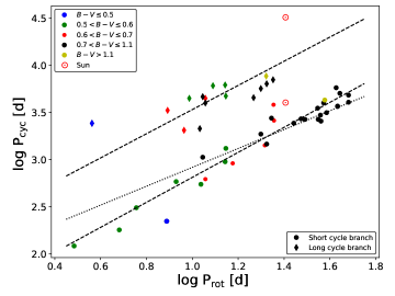
Figure 1: Logarithms of cycle period versus logarithms of rotation period for the sample stars. Here, the two branches are labelled with different signs and the different $B-V$ ranges are colour-coded. Furthermore, the dashed lines are depicted the estimated trends in the range $0.5\leq B-V\leq 1.1$ of the cycle-rotation relations in both branches and the dotted line represents the trend with a fixed slope 1 for the short-cycle branch.

4 The empirical cycle-rotation connection

In this section, we study the connection between the observed activity cycle and the rotation periods. We note that the number of available data points are different for the aforementioned two branches. In total, we have 34 cycles on the short-cycle branch, yet on the long-cycle branch, we have only 17 cycles at our disposal. Accordingly, the relations for the latter are far more uncertain. Nevertheless, for the sake of completeness, we include also the long-cycle branch in this study. Furthermore, for our study, we used only the data in the $B-V$ range of $0.5<B-V\leq 1.1$ for reasons described in Sect. 5.1; this range contains the vast majority of our data, and inside this reduced $B-V$ range, we have 32 cycles on the short-cycle branch and 15 on the long-cycle branch.

We begin this investigation with the short- and long-cycle branches and in trying to find its empirical relation between the rotation and cycle periods. For this, we try a linear relation between the logarithmic cycle period and logarithmic rotation periods. Physically, this tests a power law relation between these quantities as such. For the question, whether any additional parameters would be needed, we then perform a principal component and a factor analysis. Different approaches are compared as how the arrive at statistically acceptable descriptions, by fixing the slope between cycle and rotation periods at unity on the one hand and letting the slope vary freely on the other hand, and introducing additional parameters. For these studies, we use only the cycles on the short-cycle branch because the number of cycles on the long-cycle branch is rather limited.

4.1 Power law relations between $P_{cyc}$ and $P_{rot}$

Here, we briefly discuss the power law relations between the cycle and rotation periods in both cycle branches, which become linear relations in the logarithmic variables.

4.1.1 Short-cycle branch

We begin our study with the empirical relation between the (logarithmic) cycle lengths and rotation periods, with the aim to check, whether $P^{S}_{cyc}\propto P_{rot}$ is valid, as suggested by Eq. 6 (with the index ${S}$ labelling the periods on the short-cycle period branch). Noyes et al. (1984b) used the inverse cycle period and inverse Rossby number to study the cycle-rotation relation and derived the relation $P^{S}_{\rm{cyc}}\propto P_{\rm{rot}}^{1.25\pm 0.54}$, which is consistent within the uncertainty with the theoretical prediction by Stix (1976) and also by Tuominen et al. (1988).

In Fig. 1, we plot (in a double-logarithmic representation) the measured cycle periods versus the rotational periods of our sample stars. Since the theoretical expectation given by Eq. 6 suggests a linear relation viz:

$$\log P_{\rm{cyc}} \approx a+n\log P_{\rm{rot}},$$ (7)

we then test whether the empirical slope is consistent with $n=1$. Consequently, we fix $n$ at unity and optimised only the constant $a$ via a leasts-square fit, obtaining a=1.918$\pm$0.027; the resulting relation is illustrated by the dotted line in Fig. 1.

Clearly, this regression with $n=1$ does not fit the short periods. Next, we perform a least-squares fit treating also the slope $n$ as a free parameter, and obtain the relation

$$\log P^{S}_{\rm{cyc}}[d]=(1.488\pm 0.092)+(1.324\pm 0.067)\log P_{\rm{rot}}[d],$$ (8)

and plot this as the dashed line in Fig. 1. To quantify the remaining scatter of this best-fit empirical relation, we compute the relative deviation ($(P^{\rm{S}}_{\rm{cyc}}-cal(P^{\rm{S}})_{\rm{cyc}})/P^{\rm{S}}_{\rm{cyc}}$ = $\Delta$P${}_{\rm{cyc}}^{S}/$P${}_{\rm{cyc}}^{S}$), where $cal(P^{\rm{S}})_{\rm{cyc}}$ is the calculated cycle period and obtain a standard deviation ($\sigma$) of 0.24.

Furthermore, we calculated the expected solar cycle period with this relation and obtain a period of 6.1${}^{+2.2}_{-1.6}$ yr, which differs from the well-established real mean solar cycle period of 11 years. Furthermore, the best-fit slope of 1.324 is obviously inconsistent with theoretical considerations described in Sect. 2.

4.1.2 Long-cycle branch

We now turn to the relation between cycle periods and rotation periods for the cycles located on the long-cycle branch. In Fig. 1, the available cycle and rotation period measurements are also plotted on a double-logarithmic scale. As for the cycles on the short-cycle branch, we assume a linear relation between the (logarithmic) quantities and using a least-squares fit, we arrive at the expression:

$$\log P^{L}_{\rm{cyc}}[d]=(2.22\pm 0.38)+(1.28\pm 0.33)\log P_{\rm{rot}}[d],$$ (9)

depicted as a dashed line in Fig. 1. Next, we compute the relative deviation ($\Delta P_{\rm{cyc}}^{L}/P_{\rm{cyc}}^{L}$) and obtain a standard deviation of 40$\%$, a value about a factor of $\sim$2 larger than the standard deviation on the short-cycle branch. Furthermore, the absolute value of the slope is consistent with the slope in the relation for the short-cycle branch (see Eq. 8).

Therefore, we conclude that the slope of main trends for both branches are equal and a similar result was found by Böhm-Vitense (2007). However, the error of the slope is so large that this slope is also consistent with unity within the error margin. To classify and assess this large error, the small number of used cycle periods must be taken into account; thus, it is important to find more cycles that include the corresponding rotation periods located on the long-cycle branch.

Finally, we computed the expected solar Gleissberg cycle using our derived relation (see Eq. 9) and obtained a cycle period of 31${}^{+91}_{-23}$ yr; the large error of this period reflects the large uncertainties of the cycle-rotation relation for the long-cycle branch and, hence, the quantitative predictions are not particularly meaningful.

4.2 Principal component and factor analysis of the $\log\leavevmode\nobreak\ P^{S}_{cyc}$ over $\log\leavevmode\nobreak\ P_{rot}$ relation

We now consider the question of whether additional parameters are required to describe the relation between cycles and rotation periods. From Fig. 5, it is obvious that different spectral types cover different period ranges and, furthermore, the empirical relations between cycle length and rotation period taken in individual B-V ranges differ from each other. This suggests the possibility of two kinds of effects of $B-V$: a dependence of the rotation periods themselves on $B-V$ and a dependence of the observed relation between cycle length and rotation period.

To test whether any such $B-V$ dependence is significant or not, we perform a principal component and factor analysis. Factor analysis is a well established method to investigate how many independent (or latent) variables exist in a given data set. In our specific case, we have at our

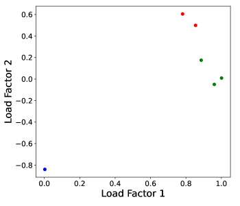
Figure 2: Factor loadings of the variables for activity (blue), rotation and cycle periods (red), and colour, convection zone depth and convective turnover time (green).

disposal the measurements of the rotation period and cycle periods, the stellar colour, depth of the convection zone, and convective turnover time, as well as the activity as measured by $R^{+}_{HK}$ (i.e. six parameters for each star). Factor analyses then attempt to describe six corresponding variables $X_{1},...X_{6}$ for each star in terms of a smaller number of variables $Y_{1},...Y_{k}$. In a first step, it is determined how many of these latent variables are in fact required to improve the residuals; for all of our analyses, we used the FactorAnalyzer package in Python.

We used normalised variables and verified that the correlation matrix of the data is not equal to the identify matrix using Bartlett’s test for sphericity; we then used the Kaiser-Meyer-Olkin (KMO) criterion to assess whether the given data is suitable for factor analysis. We then proceeded to determine the eigenvalues and eigenvectors of the correlation matrix. Applying the KMO criterion, we find two eigenvalues in excess of unity and we may therefore assume that two latent variables exist.

With the corresponding eigenvectors, we can proceed to compute the factor loadings of the six original variables in terms of the two latent variables; the result is shown in Fig. 2. We can recognise that the first loading factor provides large loadings for the variables colour, convection zone depth, and convective turnover time, while the second factor provides large loadings for the variables for activity as well as the rotation and cycle periods. It is therefore recommend that one of the two latent variables be associated with the property of ’activity’, the other one with the property of ’stellar structure’.

These results are corroborated by a principal component analysis, which shows that the introduction of a second variable, for example, the $B-V$ colour index, to describe the relation $P_{\rm{cyc}}$ versus $P_{\rm{rot}}$ reduces the total data variance by $\sim 10\%$ and is, hence, justified.

We finally note that for main sequence stars, both the convective turnover time ($\tau_{c}$) and the relative depth of the convection zone ($d_{cz}$), are strongly correlated with the stellar colour, as demonstrated in Fig. 3, where $\tau_{c}$ and $d_{cz}$ are plotted vs. $B-V$ colour index for our sample stars. We note that the $B-V$ colour is quite similar for both parameters; the only outlier is the star HD 103095, which has a very low metalicity that leads to an opacity and, hence, the depth of convection zone is different from that of the other stars.

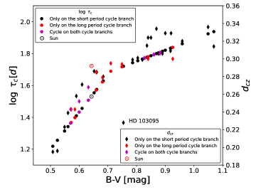
Figure 3: Convective turnover time ($\tau_{c}$) and the relative depth of the convection zone ($d_{cz}$) versus $B-V$ [mag]; the data for $\tau_{c}$ are a labelled as dots and $d_{cz}$ as diamonds; the colour-coding of the data indicates on which branch the corresponding cycle is located.

4.2.1 Cycle-rotation period relation with unity slope and additional parameters

In the following, we describe our attempts to improve the empirical cycle-rotation period relations by considering further parameters and to check the residuals from the derived cycle period expectations against the observed stellar cycle periods. For this purpose, we start again (following the theoretical expectations outlined in Sec. 2) by assuming a direct proportionality between the logarithmic cycle and rotation periods with slope unity, but now improving it with an additional parameter, namely: the $B-V$ colour index, the relative depth of the convection zone, and the convective turnover time.

We first considered the empirical dependence of the observed cycle periods on these three parameters; for an illustration, see the plots shown in Fig. 4(a-c). As is evident to the eye, a clear correlation between the cycle period and each of these three parameters exists. To remove any indirect effects of the rotation period, we considered the quantity $log(P_{\rm{cyc}}/P_{\rm{rot}})$ and studied its dependence on those three parameters; Fig. 4(d-f) gives an idea of these dependences and demonstrates a clear correlation between the logarithmic period differences and the chosen parameters. By removing the effect of the rotation, the correlation between $log(P_{\rm{cyc}}/P_{\rm{rot}})$ and those three parameters becomes smaller when compared to the correlation between $log(P_{\rm{cyc}})$ and those three parameters, which is also visible in Fig. 4. Nevertheless, the correlations between $log(P_{\rm{cyc}}/P_{\rm{rot}})$ and those three parameters have a significance of at least of 95$\%$. In the following, we discuss these dependences individually.

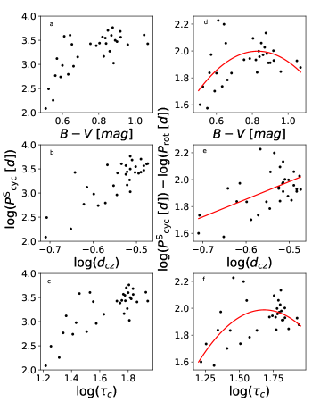
Figure 4: Correlation between logarithm of the cycle period and the colour index $B-V$, relative depth of the convection zone and convective turnover time. Left panels: Logarithm of the cycle period versus the colour index $B-V$ in panel a, versus the relative depth of the convection zone in panel b, and versus the convective turnover time in panel c. Right panels: Difference between the logarithm of the cycle period and the logarithm of the rotation period versus the colour index $B-V$ is shown in panel d, versus the relative depth of the convection zone in panel e and the convective turnover time in panel f. The red solid line in panels d to e shows the estimated trend between both values; see text for details.

4.2.1.1 $B-V$ colour index

We first considered a direct dependence of $log(P_{\rm{cyc}}/P_{\rm{rot}})$ on the $B-V$ colour index. Figure 4(d) suggests a quadratic dependence and a least-squares analysis results in the best-fit expression:

$$\log(P^{S}_{cyc}) = (1.50\pm 0.12)+\log(P_{rot})$$

$$+(2.32\pm 0.75)X+(-2.7\pm 1.0)X^{2},$$

where we define $X=B-V-0.4$, In Fig. 4d, the curve described by Eq. 4.2.1.1 is plotted with the red line.

4.2.1.2 Relative depth of the convection zone

We now assume a direct proportionality between $log(P_{\rm{cyc}}/P_{\rm{rot}})$ and the (logarithmic) relative depth of the convection zone, and (again) a least-squares analysis results in the best-fit expression:

$$\log(P^{S}_{cyc})=(2.64\pm 0.20)+\log(P_{rot})+(1.31\pm 0.36)\log(d_{cv}),$$ (11)

with $d_{cz}$ denoting the relative depth of the convection zone. In Fig. 4, the curve described by Eq. 11e is again plotted with the red line.

4.2.1.3 Convective turnover time

Finally, we compared $log(P_{\rm{cyc}}/P_{\rm{rot}})$ and the (logarithmic) convective turnover time. From Fig. 4(f), we assume a quadratic dependence and a least-squares analysis results in the best-fit expression:

$$\log(P^{S}_{cyc}) = (1.60\pm 0.09)+\log(P_{rot})$$

$$+(1.61\pm 0.51)Y+(-1.67\pm 0.65)Y^{2},$$

where we define $Y=\log(\tau_{c})-1.2$ and $\tau_{c}$ denotes the convective turnover time (in days). In Fig. 4f, the curve described by Eq. 4.2.1.3 is again plotted with the red line.

With the introduction of the empirical convective turnover time in the cycle-rotation relation, we can substitute the rotation period with the above-introduced Rossby number, which is the ratio between the rotation period and the convective turnover time. The obtained relation (see Eq. 4.2.1.3) can then be rewritten in the form: $P^{S}_{cyc}\propto Ro$.

4.2.2 Double logarithmic cycle-rotation relation with variable slope and a $B-V$ splitting

In this subsection, we analyse how much it is possible to improve the empirical cycle-rotation relations with a variable slope (i.e. not fixed at unity) by considering the possible $B-V$ colour index dependence.

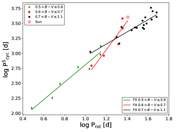
Figure 5: Logarithms of short-cycle branch periods are plotted over the logarithm of rotation period. Different $B-V$ ranges are colour coded and the solid lines depict the estimated empirical relations of individual $B-V$ ranges, which discussed in Sec. 4.2.2.

To check the $B-V$ dependence, we split the data into different $B-V$ ranges, labelled by different colours and symbols in Figs. 1 and 5. We also point out (in Sect. 5.1 and Fig. 7) a clear splitting into these $B-V$ ranges. From an inspection of Fig. 5, it is obvious that different spectral types cover different period ranges. Next, we estimate the trends between $\log P^{S}_{cyc}$ and $\log P_{rot}$ with the linear model (see Eq. 7) through a least-squares fit in those three $B-V$ ranges. The results are listed in Table 2, including the number of data points in each $B-V$ range. This listing reveals differences between the individual $B-V$ ranges. For the later spectral types, the derived best-fit slopes are indeed near unity, whereas the slopes become greater than unity for the earlier spectral types, suggesting again that the trend between the cycle period and the rotation period depends on spectral type and, thus, on $B-V$.

Next, we computed the relative deviation ($\Delta$P${}_{\rm{cyc}}^{S}/$P${}_{\rm{cyc}}^{S}$) to check the reduction of the remaining scatter compared to the cycle-period relation (see Eq. 8) and obtained a standard deviation ($\sigma$) of 0.20, namely, a reduction in the scatter of $\approx$15$\%$.

Finally, we calculated the solar cycle period with the obtained relation for the $B-V$ range from 0.6 to 0.7, listed in Table 2, and we obtained a cycle period of 9.6${}^{+31.5}_{-7.4}$ yr. However, due to the large error in the slope, the error margins of this value are extremely large, thus making this cycle period very uncertain. Nevertheless, this calculated period is consistent with the well-known 11-year Schwabe cycle and it is located in the range of the measured cycle lengths for the Schwabe cycle.

Table 2: Results of the $B-V$ trend estimation to test a possible secondary $B-V$ dependence (see Fig. 5)

$B-V$ range	No. of	a	n	$\sigma$ of
	data			$\Delta$P${}_{\rm{cyc}}^{S}/$P${}_{\rm{cyc}}^{S}$
$0.5<B-V\leq 0.6$	7	1.35$\pm$0.05	1.46$\pm$0.08	0.20
$0.6<B-V\leq 0.7$	6	0.23$\pm$0.13	2.36$\pm$0.44	0.29
$0.7<B-V\leq 1.1$	19	1.93$\pm$0.06	1.02$\pm$0.04	0.17

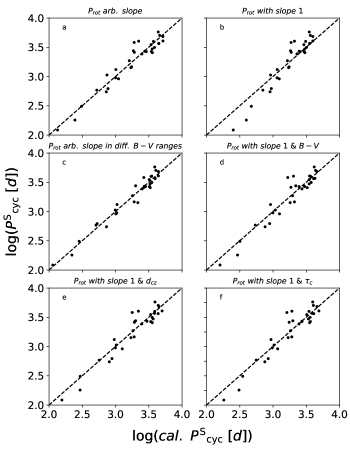
Figure 6: Measured versus calculated cycle period as the basis of the comparison among the different models. Panel a: Linear model (Eq. 7) with a best-fit slope for $\log(P_{rot})$. Panel b: Linear model (Eq. 7) with a slope of 1 for $\log(P_{rot})$. Panel c: Linear model (Eq. 7) with a best-fit slope for $\log(P_{rot})$ for different $B-V$ ranges. Panel d: Model (Eq. 4.2.1.1) with a slope of 1 for $\log(P_{rot})$ and $B-V$ term. Panel e: Model (Eq. 11) with a slope of 1 for $\log(P_{rot})$ and the relative depth of the convection zone. Panel f: Model (Eq. 4.2.1.1) with a slope of 1 for $\log(P_{rot})$ and the convective turnover time.

4.3 Summary of the different approaches to the $\log\leavevmode\nobreak\ P^{S}_{cyc}$ versus $\log\leavevmode\nobreak\ P_{rot}$ relation

In our regression analyses, we considered different models that make different assumptions on the proportionality between the logarithmic cycle and rotation periods and additional stellar parameters. In this subsection, we compare how well the different empirical representations reproduce the actual observed cycle periods (cf., Fig. 6). To quantify the ‘goodness of fit’ of any empirical relation by its residuals, we used the relative differences between observed and measured periods, listed in Table 3.

Table 3: The relative deviations of the different $P^{S}_{cyc}$ versus $P_{rot}$ models

Model	Fig. 6	$\sigma$ of $\Delta$P${}_{\rm{cyc}}^{S}/$P${}_{\rm{cyc}}^{S}$
	panel
$P_{rot}\leavevmode\nobreak\ arb.\leavevmode\nobreak\ slope$	a	0.24
$P_{rot}\leavevmode\nobreak\ with\leavevmode\nobreak\ slope\leavevmode\nobreak\ 1$	b	0.40
$P_{rot}\leavevmode\nobreak\ arb.\leavevmode\nobreak\ slope\leavevmode\nobreak\ in\leavevmode\nobreak\ diff.\leavevmode\nobreak\ B-V\leavevmode\nobreak\ ranges$	c	0.20
$P_{rot}\leavevmode\nobreak\ with\leavevmode\nobreak\ slope\leavevmode\nobreak\ 1$ & $B-V$	d	0.27
$P_{rot}\leavevmode\nobreak\ with\leavevmode\nobreak\ slope\leavevmode\nobreak\ 1$ & $d_{cz}$	e	0.28
$P_{rot}\leavevmode\nobreak\ with\leavevmode\nobreak\ slope\leavevmode\nobreak\ 1$ & $\tau_{c}$	f	0.29

An inspection of Table 3 shows that the best-fit slopes (hence, different from unity) in the cycle-rotation relation already yield a very good description, which can be further improved upon by splitting up the data into different colour regimes. However, enforcing a slope of unity always leads to poorer results, even though they can still be improved by distinguishing between different $B-V$-colours, the relative depth of the convection zone, or convective turnover time (all functions of $B-V$-colour). However, none of these additional considerations allows for a description that produces the same fit quality of those obtained with the best-fit slopes.

Table 4: Results of the overall F-tests

Model	F-value	p-value
compare to $P_{rot}\leavevmode\nobreak\ with\leavevmode\nobreak\ slope\leavevmode\nobreak\ 1$
$P_{rot}\leavevmode\nobreak\ with\leavevmode\nobreak\ slope\leavevmode\nobreak\ 1$ & $B-V$	2.81	0.0032
$P_{rot}\leavevmode\nobreak\ with\leavevmode\nobreak\ slope\leavevmode\nobreak\ 1$ & $d_{cz}$	2.53	0.0063
$P_{rot}\leavevmode\nobreak\ with\leavevmode\nobreak\ slope\leavevmode\nobreak\ 1$ & $\tau_{c}$	3.81	0.0003
compare to $P_{rot}\leavevmode\nobreak\ with\leavevmode\nobreak\ slope\leavevmode\nobreak\ 1$
$P_{rot}\leavevmode\nobreak\ arb.\leavevmode\nobreak\ slope$	5.18	9.90$\cdot 10^{-6}$
compare to $P_{rot}\leavevmode\nobreak\ arb.\leavevmode\nobreak\ slope$
$P_{rot}\leavevmode\nobreak\ arb.\leavevmode\nobreak\ slope\leavevmode\nobreak\ in\leavevmode\nobreak\ diff.\leavevmode\nobreak\ B-V\leavevmode\nobreak\ ranges$	4.31	0.0002

To test for the significance of the reduction of the residuals by use of best-fit slopes compared to a reference model, we used the overall F-test for either type of empirical relation. In this overall F-test, the different numbers of degrees of freedom are considered, so that a comparison of the models independent of the degrees of freedom is possible. The resulting p-values give the confidence level of the reduction of the relative deviations. In all cases, the obtained p-values indeed suggest a significant improvement over the relations based on unity slopes.

In summary, these overall F-tests suggest that the best empirical representation of the cycle-rotation relation is a power law (i.e. with a non-unity best-fit slope in the double-logarithmic diagram) when distinguishing between different $B-V$ ranges. The emerging $B-V$ dependence has two possible reasons: while the $B-V$ dependence of the cycle period is well known from the activity-rotation relation, the second $B-V$ dependence (i.e. how much the cycle period actually depends on rotation period) seems to be related to stellar structure.

5 Rossby number as a natural parameter for the cycle-rotation relation

In Sect. 4.2.1.3, we introduce the convective turnover time in the cycle-rotation relation, which opens up the possibility of using the Rossby number as the physical parameter, instead of the rotation period. In the landmark paper by Noyes et al. (1984a), a simple (colour-independent) rotation-activity relation was found once the rotation periods are ‘parameterised’ by the Rossby number. Therefore, we decided to study the possible improvements coming from the use of the Rossby number.

Using the Rossby number to ‘scale’ the actual rotation periods leads to a shift onto a comparable rotation scale, irrespective of colour. To compute the Rossby numbers for our sample stars, we used the prescription for the calculation of the empirical convective turnover time derived in (Mittag et al. 2018); with this empirical definition of the convective turnover time, a clear definition range between 0 and 1 for the Rossby number (Mittag et al. 2018) can be obtained. This approach is consistent with dynamo modelling, which suggests that cyclic activity is obtained only for Rossby numbers smaller than one, equivalent to a dynamo number larger than unity.

Furthermore, taking into account the best empirical representation above is of the form so that $P^{S}_{\rm{cyc}}\propto P_{\rm{rot}}^{n}$, we use the same type of ansatz:

$$P^{S}_{\rm{cyc}} \propto A\times Ro^{n},$$ (13)

where the constant, $A,$ denotes some timescale. We used the convective turnover time, $\tau_{c}$, as the timescale for this constant, $A$.

5.1 Empirical $P^{S}_{\rm{cyc}}-Ro$ relation

In the upper panel of Fig.  7, we plot the cycle periods versus the corresponding Rossby numbers for our sample stars in a double logarithmic scale; it is clear that the introduction of the Rossby number leads to a horizontal shift of the data points shown in Fig. 5, which then changes the simple cycle-rotation period relation described by Eq. 8. However, a re-scaling of the rotation periods with the empirical convective turnover time leads to an almost identical Rossby number range for the different stellar samples, which serves as an argument in favour of this approach. Furthermore, the upper panel of Fig.  7 suggests that the cycle periods are divided into three main $B-V$ ranges, $0.5<B-V\leq 0.6$, $0.6<B-V\leq 0.7$ and $0.7<B-V\leq 1.1.$ Therefore, we used this $B-V$ splitting for our study in Sect. 4.2.2 and labelled these ranges in Figs. 1 and 5. Also, the trends between the cycle periods and Rossby numbers in these $B-V$ ranges differ; two data points are clearly outside of these $B-V$ ranges and these two points are not considered further in our study; thus, the numbers of the used cycle periods is reduced from 34 to 32 cycles.

We then fit the data in the three $B-V$ ranges using the logarithmic form of Eq. 13 and a simple linear least-squares fit that takes the form:

$$\log P^{S}_{\rm{cyc}} = \log(A_{i})+n^{S}_{i}\log Ro,$$ (14)

where the index $i$ labels the different $B-V$ ranges. Thus, we obtain the results listed in Table 5. Also, the derived regression curves are shown as solid coloured lines in Fig. 7.

A comparison of the slopes in Table 2 shows that these are similar within the error margins, except for the colour range of $0.5<B-V\leq 0.6$. Similarly to the results obtained in Sect. 4.2.2, these findings again suggest a $B-V$ dependence of the trends. We note that for the stars of earlier spectral types, the derived slopes are not consistent with unity, while for the later types, they are consistent once the Rossby number is used as a parameter.

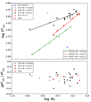
Figure 7: Logarithm of cycle periods on the short-cycle branch versus the logarithm of the Rossby number. Upper panel: Cycle period against Rossby number for cycles on the short-period (inactive) branch; different colours and symbols indicate the different $B-V$ ranges. The solid-coloured lines show the respective empirical relations, with colours indicating the different $B-V$ ranges. Lower panel: Relative deviation ($\Delta P^{\rm{S}}_{\rm{cyc}}/P^{\rm{S}}_{\rm{cyc}}$) versus the logarithm of the Rossby number. The green points label the stars within the $B-V$ range of $0.5<B-V\leq 0.6$, the red points stars within $0.6<B-V\leq 0.7$, and the black points those within $0.7<B-V\leq 1.1$.

Table 5: Results of the $B-V$-specific empirical relations (see Fig. 7)

B-V range	No. of	$\log(A)$	$n^{S}$	$\sigma$ of
	data			$\Delta$P${}_{\rm{cyc}}^{S}/$P${}_{\rm{cyc}}^{S}$
$0.5<B-V\leq 0.6$	7	3.55$\pm$0.05	2.03$\pm$0.09	0.09
$0.6<B-V\leq 0.7$	6	3.86$\pm$0.03	2.31$\pm$0.10	0.07
$0.7<B-V\leq 1.1$	19	3.79$\pm$0.04	1.07$\pm$0.13	0.19

Using the fit results displayed in Table 5, we can again calculate the relative deviations ($\Delta P^{\rm{S}}_{\rm{cyc}}/P^{\rm{S}}_{\rm{cyc}}$), plotted in the lower panel of Fig. 7. The three $B-V$ ranges are again colour-coded, green points denote stars in the $B-V$ range of $0.5<B-V\leq 0.6$, red points stars in $0.6<B-V\leq 0.7$, and black points those in $0.7<B-V\leq 1.1$.

To evaluate the scatter of $\Delta P^{\rm{S}}_{\rm{cyc}}/P^{\rm{S}}_{\rm{cyc}}$, we calculated the standard deviation of $\Delta P^{\rm{S}}_{\rm{cyc}}/P^{\rm{S}}_{\rm{cyc}}$ and obtained a scatter value of 0.15 for all stars, implying an average deviation of 15 $\%$ for the used stars. Compared to the remaining scatter for the relation Eq. 8, we see the residual deviation is clearly decreased by the use of the Rossby number as parameter.

Further support for this approach comes from the solar 11-year cycle. Using the stellar relation that is valid for the solar $B-V$ colour range, we find an expected cycle period of 10.2${}^{+0.8}_{-0.7}$ yr, which indeed nicely matches the 11-year Schwabe cycle. Hence, in the framework of the empirical cycle-rotation relation presented here, the solar 11-year Schwabe cycle follows the trend between the $\log P^{S}_{cyc}$ and $\log Ro$ very well. Consequently, in this relation, the solar 11-year Schwabe cycle is no longer an outlier as in the relation between the $\log P^{S}_{cyc}$ and $\log P_{rot}$ (cf. Fig. 1).

5.2 Physical interpretation of the $P^{S}_{\rm{cyc}}-Ro$ relation

Up to this point, we have look at the relationship between the cycle period and Rossby number on purely empirical grounds. In our factor analysis (described in Sect. 4.2), we found that the convective turnover time and the relative depth of the convection zone can be viewed as latent variables in the cycle-rotation relation. Furthermore, in Sects. 4.2.1.3 and 4.2.1.2, we consider the significance of these additional parameter in the cycle-rotation relation, with the exponent of the rotation period fixed at unity. Therefore, we may assume that these hitherto unconsidered parameters are to be found again in the constant A in Eq. 13.

To test the effects of the introduction of $\tau_{c}$ on the $P^{S}_{\rm{cyc}}-Ro^{n^{S}_{i}}$ relation, we compared ( in Fig. 8) the values of $\log P^{S}_{\rm{cyc}}$ with $\log(\tau_{c}Ro^{n^{S}_{i}})$, with the coefficients $n^{S}_{i}$ listed in Table 5. It is evident that that the splitting between different B-V ranges (as seen in Fig. 7) has mostly disappeared and the relation between between $\log P^{S}_{\rm{cyc}}$ and $\log(\tau_{c}Ro^{n^{S}_{i}})$ is linear. However, it is also visible that the different $B-V$ ranges are slightly shifted around the mean trend, with the cooler stars lying mostly below and the hotter stars lying mostly above the regression line. We assume that these effects are caused by the hitherto unconsidered length scale of the turbulence (cf., Eq. 6), and, furthermore, we assume that this turbulence length scale ($l/R_{\star}$) is representative for the relative depth of the convection zone where the dynamo is located. Assuming that the dynamo is located at the bottom of the convection zone, we may use $d_{cz}$ instead of $l/R_{\star}$. Finally, we remark that HD 103095 shows a strong deviation in the relative depth of the convection zone-colour relation when compared to the other stars (see Fig. 3); therefore, we excluded this star from this analysis.

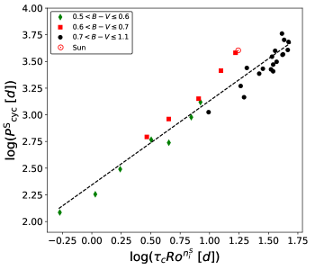
Figure 8: Comparison of $\log P^{S}_{\rm{cyc}}$ with $\log(\tau_{c}Ro^{n^{S}_{i}})$, where the $B-V$ ranges are colour-coded.

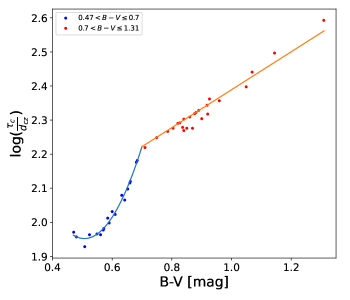
Figure 9: Logarithm of the ratio of the convective turnover time and relative depth of the convection are shown. Solid-coloured line depicts the estimated trend. Solid-blue line depicts the $B-V$ range of $0.47\leavevmode\nobreak\ <\leavevmode\nobreak\ B\leavevmode\nobreak\ -V\leavevmode\nobreak\ \leq\leavevmode\nobreak\ 0.7$ and the solid-red line shows the range of $0.7\leavevmode\nobreak\ <\leavevmode\nobreak\ B\leavevmode\nobreak\ -V\leavevmode\nobreak\ \leq\leavevmode\nobreak\ 1.31$.

Accordingly, we assume that the ratio of $\tau_{c}$ and $d_{cz}$ is contained in the constant $A$ introduced above and show this ratio of our sample stars in Fig. 9. Physically, this ratio acts as the inverse of velocity, describing the speed of the convective overturn in a convection zone; naturally, this velocity depends on $B-V,$ such that:

$$A \sim \left(\frac{\tau_{c}}{d_{cz}}\right)=v^{-1}_{dcz}(B-V).$$ (15)

In Fig. 9, a clear change is apparent at the level of colour $B-V\approx 0.7$. Hence, we split the data at B-V = 0.7 and derived two relations via a least-squares fit: for the $B-V$ range $0.47<B-V\leq 0.7$, we obtain:

$$v^{-1}_{dcz} = (2.035\pm 0.021)$$ (16)

$$-(1.55\pm 0.24)X+(7.25\pm 0.65)X^{2},$$

where $X=(B-V-0.4)$, and for the $B-V$ range $0.7\leavevmode\nobreak\ <\leavevmode\nobreak\ B\leavevmode\nobreak\ -\leavevmode\nobreak\ V\leavevmode\nobreak\ \leq\leavevmode\nobreak\ 1.31$, we obtain:

$$v^{-1}_{dcz} = (2.222\pm 0.095)+(0.557\pm 0.016)X,$$ (17)

where $X=(B-V-0.7)$. For this trend estimation, we also used the four data points outside the $B-V$ range $0.5<B-V\leq 1.1$. The relations obtained in this way are depicted as a solid line in Fig. 9. In the next section, we use these relation to derive our final $P^{S}_{\rm{cyc}}-Ro$ relation.

5.3 Final $P^{S}_{\rm{cyc}}-Ro$ relation for the short-cycle branch

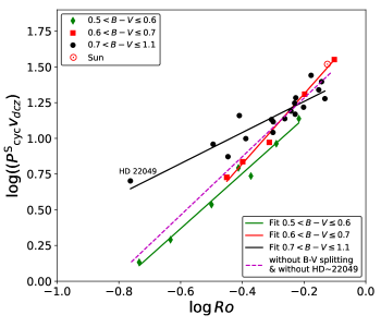
Figure 10: Ratio of the cycle period and constant $A$ (see Eq. 15) versus Rossby number in a double logarithmic scale, where the $B-V$ ranges are colour-coded. Furthermore, estimated trends in these $B-V$ ranges are depicted as solid and coloured lines.

Using the relations in Eqs. 16 and 17, we can compute the ratio of $\tau_{c}$ and $d_{cz}$ for all stars, scale the corresponding cycle period with this value, and plot $\log(P^{S}_{\rm{cyc}}v_{dcz}(B-V))$ versus $\log(Ro)$ in Fig. 10 (again colour-coding the three main $B-V$ ranges). Fig. 10 shows a linear relation between $\log(P^{S}_{\rm{cyc}}v_{dcz}(B-V))$ and $\log(Ro)$ with some ‘outliers’; alternatively, by introducing B-V ranges, we find linear relations but with different parameters. In the following, we study these relations using these approaches.

5.3.1 Final fit without $B-V$ splitting

In Fig. 10, we note a single blatantly outlying data point (at $\log Ro\approx-0.76$ and $\log(P^{S}_{\rm{cyc}}v_{dcz}(B-V))\approx 0.7$), which refers to HD 22049 (=eps Eri). This single data point of HD 22049 has a huge impact on our fit of the trend. Considering this data point as outlier here and ignoring it in our least-squares fit, we obtain:

$$\log\left(\frac{P^{S}_{\rm{cyc}}d_{cz}}{\tau_{c}}\right) = \log\left(P^{S}_{\rm{cyc}}v_{dcz}\right)=$$ (18)

$$(1.692\pm 0.049)+(2.05\pm 0.14)\log Ro.$$

This result is plotted as magenta dotted line in Fig. 10.

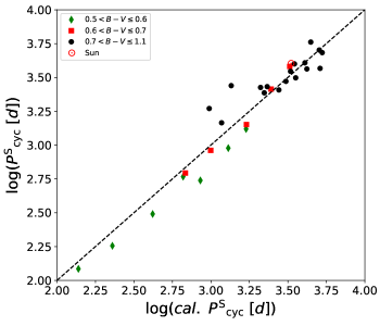
Figure 11: Comparison of the observed and calculated cycle periods from the relation of Eq. 20, the $B-V$ ranges are colour-coded. The dashed line depicts the identity.

Next, we compare the observed and calculated cycle periods with the expression

$$P^{S}_{\rm{cyc}} = 10^{1.692\pm 0.049}v^{-1}_{dcz}Ro^{2.05\pm 0.14},$$ (19)

and we plot the results in Fig. 11. Although the three main B-V ranges in this trend estimation have not been considered, we colour-coded these three $B-V$ ranges to check whether any possible $B-V$ dependencies or systematics remain. A inspection by eye of Fig. 11 shows two possible cases where such $B-V$ systematics do indeed remain. First, it is clear that all data points for the $B-V$ range $0.5<B-V\leq 0.6$ are located below the regression curve which indicates that the calculated cycle periods are systematically overestimated. Second, in the $B-V$ range $0.7<B-V\leq 1.1,$ the data seem to display a different trend.

To quantify the deviation between the observed and calculated cycle periods, we determined the standard deviation of the relative deviations $\Delta P^{\rm{S}}_{\rm{cyc}}/P^{\rm{S}}_{\rm{cyc}}$ and obtain 0.24. This value is similar the standard deviation of $\Delta P^{\rm{S}}_{\rm{cyc}}/P^{\rm{S}}_{\rm{cyc}}$ for the pure cycle-rotation relation (see Eq. 8). Thus, the relation in Eq. 19 does not provide a (statistically) better cycle-rotation connection than pure cycle-rotation relation (see Eq. 8). However, for the Sun, we find a cycle period of 9.0${}^{1.2}_{1.0}$ yr close to the 11-year cycle in contrast to the 6.1${}^{+2.2}_{-1.6}$ yr cycle period estimated from Eq. 8. Therefore, in this context the Sun is no longer an outlier, yet we have no explanation for the ‘strange’ properties of $\epsilon$ Eri.

5.3.2 Final fit with $B-V$ splitting

Retaining all data points in the sample, it is not possible to find a single (linear) relationship; rather, we find that a possible $B-V$ dependence remains. As made clear from Fig. 10, in the three main colour-coded $B-V$ ranges, the $\log(P^{S}_{\rm{cyc}}v_{dcz}(B-V))$ values show a linear dependence. Assuming then a linear relation in each B-V range of the form:

$$\log\left(\frac{P^{S}_{\rm{cyc}}d_{cz}}{\tau_{c}}\right)=\log\left(P^{S}_{\rm{cyc}}v_{dcz}\right) = a^{S}_{i}+n^{S}_{i}\log Ro,$$ (20)

where the index $i$ labels the different $B-V$ ranges, we derived the parameters $a^{S}_{i}$ and $n^{S}_{i}$ via a least-squares fit for the different $B-V$ ranges. In Fig. 10, these regressions are shown as solid and coloured lines, and the respective fit parameters are listed in Table 6.

We note that with this approach, HD 22049 is well fitted in the trend of the $B-V$ range $0.7<B-V\leq 1.1$ and the fit results do not depend on whether or not HD 22049 is included or not. Based on these results, we modelled the observed cycle periods using the expression:

$$P^{S}_{\rm{cyc}} = \frac{10^{a^{S}_{i}}}{d_{cz}}\tau_{c}Ro^{n^{S}_{i}}=10^{a^{S}_{i}}v^{-1}_{dcz}Ro^{n^{S}_{i}},$$ (21)

where $10^{a^{S}_{i}}$ is a constant and $n^{S}_{i}$ is the exponent of the Rossby number, and the index, $i,$ labels the different $B-V$ ranges.

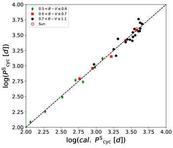
Figure 12: Deviations of the observed stellar cycles from the relation of Eq. 21, the $B-V$ ranges are colour coded. The dashed line depicts the identity.

Table 6: Estimated parameters for Eq. 20

B-V range	No. of	$a^{S}$	$n^{S}$	$\sigma$ of
	data			$\Delta$P${}_{\rm{cyc}}^{S}/$P${}_{\rm{cyc}}^{S}$
$0.5<B-V\leq 0.6$	7	1.53$\pm$0.05	1.93$\pm$0.11	0.10
$0.6<B-V\leq 0.7$	6	1.80$\pm$0.04	2.44$\pm$0.12	0.08
$0.7<B-V\leq 1.1$	18	1.48$\pm$0.04	1.09$\pm$0.12	0.17

In Fig. 12, the observed cycle periods are directly compared with the calculated ones from the derived best-fit relation in Eq. 21 with the parameters listed in Table 6. These values are listed in Table 1. In Fig. 12, the three $B-V$ ranges are labelled with the same colour-coding as in Fig. 7. Figure 12 demonstrates that the calculated cycle periods are very well distributed around the identity line (plotted as a dashed line in Fig. 12).

Next, we determined the relative deviations $\Delta P^{\rm{S}}_{\rm{cyc}}/P^{\rm{S}}_{\rm{cyc}}$ and show these values as red data points in Fig. 13. Furthermore, we computed the corresponding standard deviation of $\Delta P^{\rm{S}}_{\rm{cyc}}/P^{\rm{S}}_{\rm{cyc}}$ to quantify the deviation between the observed and calculated cycle periods. The standard deviations in the three $B-V$ range are listed in Table 6. For all stars in this study, a value of 0.14 was obtained, namely, an average deviation of 14$\%$. This scatter is similar to the one obtained around the relation given by Eq. 14, implying no improvement by the inclusion of these additional parameters. However, this may simply be a consequence of the small data set available for this study. Finally, we again calculated the solar activity cycle period by the final empirical relation, which results in a calculated solar cycle period of 10.3${}^{1.1}_{1.0}$ yr. This value is fully consistent with the well-known 11-year Schwabe cycle.

In the following, we provide a brief comparison to the simple cycle-rotation relation presented in Sects. 4.1.1 and 4.2.2. Using only stars in the $B-V$ range of $0.5<B-V\leq 1.1,$ we plot the relative deviation $\Delta P^{\rm{S}}_{\rm{cyc}}/P^{\rm{S}}_{\rm{cyc}}$ for the three relations in Fig. 13, where the black data points show $\Delta P^{\rm{S}}_{\rm{cyc}}/P^{\rm{S}}_{\rm{cyc}}$ for the relation given by Eq. 8, magenta data points the $\Delta P^{\rm{S}}_{\rm{cyc}}/P^{\rm{S}}_{\rm{cyc}}$ for the relation given by Eq. 7 with the parameters listed in Table 2, and red data points $\Delta P^{\rm{S}}_{\rm{cyc}}/P^{\rm{S}}_{\rm{cyc}}$ for the relation given by Eq. 21. It is obvious that $\Delta P^{\rm{S}}_{\rm{cyc}}/P^{\rm{S}}_{\rm{cyc}}$ obtained with Eq. 8 shows a larger scatter compared to the other. Also, we can see that $\Delta P^{\rm{S}}_{\rm{cyc}}/P^{\rm{S}}_{\rm{cyc}}$ obtained with Eq. 21 show the smallest scatter. We then compared the standard deviation of the $\Delta P^{\rm{S}}_{\rm{cyc}}/P^{\rm{S}}_{\rm{cyc}}$ sets, 0.24 for the relation Eq. 8, then 0.19 for Eq. 7 and parameter listed in Table 2, and 0.14 for the relation in this section. These values are confirmed the visual observation from Fig. 13.

As a further test, the calculated cycle lengths for the solar cycle can be considered: with the simple linear relation Eq. 8, the relative deviation of the Sun is $\approx$ 45$\%$. This stands in contrast to the relative deviation of $\approx$ 13$\%$ obtained with Eq. 7 and the parameters listed in Table 2 as well as a relative deviation of $\approx$ 6$\%$ obtained using the relation derived in this section.

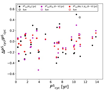
Figure 13: Relative deviations versus cycle on the inactive branch. Black data points show $\Delta P^{\rm{S}}_{\rm{cyc}}/P^{\rm{S}}_{\rm{cyc}}$ for the relation given by Eq. 8, magenta data points the $\Delta P^{\rm{S}}_{\rm{cyc}}/P^{\rm{S}}_{\rm{cyc}}$ for the relation given by Eq. 7 with parameter listed in Table 2 and red data points $\Delta P^{\rm{S}}_{\rm{cyc}}/P^{\rm{S}}_{\rm{cyc}}$ for the relation given by Eq. 21.

Finally, we tested the statistical significance of the variance reduction between the models. First, we compared the variance between the relation given by Eq. 8 and the relation derived in this section via an overall F-test, obtaining $F=15.8$. Based on this F-value, we obtained a formal p-value of 4.6$\cdot 10^{-10}$, which shows a clearly statistically significant reduction in the residual deviations between these models. Next, we compared the variance between the relation given by Eq. 7, with the given parameter from Table 2, and the relation derived in this section. Both relations have the same numbers of degrees of freedom, so that we can use a F-test where the numbers of degrees of freedom are not taken into account. We obtained an F-value of 1.91 and a corresponding formal p-value of 0.06. This p-value shows a statistically significant reduction of 94$\%$ between these models.

5.3.3 Summary and conclusions for our final $P^{S}_{\rm{cyc}}-Ro$ relation for the short-cycle branch

In this section, we explain how we derived a cycle-Rossby number relation with and without the $B-V$ splitting into three main ranges. In both relations, the convective turnover time and the relative depth of the convection zone were considered. We found that the relation without $B-V$ splitting does not describe the cycle-rotation connection any better than the simple linear relation with the rotation period does (see Eq. 8). However, the relation derived in Sect. 5.3.2, which includes the splitting into three $B-V$ ranges, shows the smallest deviation between the observed and calculated cycle period compared to the other derived relations in this work. Therefore, we conclude that this new, final relation presented in Sect. 5.3.2, based on the Rossby number parameter, describes the cycle-rotation relation much better than a simple linear relation with rotation period (see Eq. 8) and better than the linear relation with rotation period including the $B-V$ splitting (see Eq. 7 and the parameters in Table 2).

Furthermore, we conclude that the $B-V$ splitting into three ranges is important for describing the cycle-rotation relation. This $B-V$ splitting into three main $B-V$ ranges is not removed with the introduction of convective turnover time and the relative depth of the convection zone or by the ratio of these two parameters. A comparison of the slopes given in Tables 5 and 6 shows that the slopes do not change significant significantly, supporting this conclusion.

5.4 Cycles on the long-period branch versus Rossby number

In our sample, there are only 15 stars located on the long-cycle branch and in the relevant $B-V$ range of $0.5<B-V<1.1,$ the available sample is very small. Here, too, we split the data into the different $B-V$ ranges and plot the logarithm of the cycle lengths on the long-cycle (active) branch versus the logarithm of the Rossby numbers (see Fig. 14). A visual inspection of Fig. 14 suggests some evidence for differences with $B-V$.

To test and quantify any such $B-V$-specific relations, we focussed again on three main $B-V$ ranges and performed a linear least-squares fit (cf., Eq.14); the results of the fits are shown in Table 7, including the number of data points in the corresponding $B-V$ range.

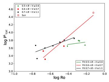
Figure 14: Logarithm of cycles on the long-cycle branch versus the logarithm of the Rossby numbers; different colours and symbols indicate data in different $B-V$ ranges. Solid coloured lines show the different relations obtained for the fitted $B-V$ ranges.

Table 7: Results of the $B-V$-specific relations for the cycles on the long-cycle branch

$B-V$ range	No. of	A	n
	data
$0.5<B-V\leq 0.6$	4	3.82$\pm$0.18	0.31$\pm$0.60
$0.6<B-V\leq 0.7$	4	4.69$\pm$0.19	1.97$\pm$0.40
$0.7<B-V\leq 1.1$	7	4.16$\pm$0.17	0.86$\pm$0.29

Given the scatter in the data on the long-cycle branch, as well as the paucity of data points and the relatively small span of covered Rossby numbers, we consider those relations relatively uncertain; this also applies to the $B-V$ range of $0.5<B-V\leq 0.6$, where the slope is consistent with zero. Furthermore, the relation for the $B-V$ range of $0.6<B-V\leq 0.7$ strongly depends on the adopted cycle value of the solar Gleissberg cycle. Therefore, we cannot obtain a meaningful trend in this $B-V$ range based on stellar data alone.

Next, we tested whether the cycle periods located on the long-cycle branch can be described in the same way as above for the short-cycle branch (see Sect. 5.3.2). In this case, the corresponding relation is:

$$P^{L}_{\rm{cyc}} = \frac{10^{a^{L}_{i}}}{d_{cz}}\tau_{c}Ro^{n^{L}_{i}}=10^{a^{L}_{i}}v^{-1}_{dcz}Ro^{n^{L}_{i}},$$ (22)

where (again) $a^{L}_{i}$ is a constant, $n^{L}_{i}$ is the exponent of the Rossby number, and the index, $i,$ labels the different $B-V$ ranges. As described in Sect. 5.3.2, we used the relations in Eqs. 16 and 17 to estimate the ratio of the convective turnover time and relative depth of the convection. Since the number of cycles on the long-cycle period branch is very limited, it is not possible to fit the data the same way as in Sect. 5.2 to obtain robust parameters for $a^{L}_{i}$ and $n^{L}_{i}$.

Instead of estimating the parameter $n^{L}_{i}$ via a fit, we used the parameters $n^{S}_{i}$ of the short-cycle branch, based on the fact that the slopes $n$ in the Eq. 14 are the same as those for the cycles on the short- and long-cycle branch (see Tables 5, 6, and 7) within the error margins, implying that an individual fit will not produce any significantly different values.

With the given $n^{S}_{i}$ values in Table 6, Eq. 22 can be transformed to $a^{L}_{i}$ and by averaging the individual values of $a^{L}_{i}$ in the corresponding $B-V$ ranges, the constants, $a^{L}_{i}$, can be obtained for the three used $B-V$ ranges. These results are listed in Table 8.

Table 8: Estimated parameters for Eq. 22

B-V range	No. of	$a^{L}$	$n^{L}$	$\sigma$ of
	data points			$\Delta$P${}_{\rm{cyc}}^{L}/$P${}_{\rm{cyc}}^{L}$
$0.5<B-V\leq 0.6$	4	2.31$\pm$0.14	1.93$\pm$0.11	0.37
$0.6<B-V\leq 0.7$	4	2.80$\pm$0.17	2.44$\pm$0.12	0.34
$0.7<B-V\leq 1.1$	7	2.00$\pm$0.10	1.09$\pm$0.12	0.24

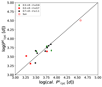
Figure 15: Comparison of the measured cycle periods on the long-cycle branch against the empirical relation given by Eq. 22 with the parameters listed in Table 8, where the $B-V$ ranges are colour-coded. The dashed line depicts the identity relation.

In Fig. 15, the measured cycle periods on the long-cycle branch are compared with the calculated cycle periods (as listed in Table 1) from the relation given by Eq. 22, with the derived parameters listed in Table 8. Inspection of these data shows they are well distributed around the identity shown as dashed line. Not unexpectedly, the scatter of these data is larger than for the data on the short-cycle period branch: we compute a standard deviation of 0.28, a factor $\sim$2 larger than the standard deviation found on the short-cycle period branch with our final, best empirical relation. Finally, we compare the Gleissberg cycle of the Sun with the expectation given by Eq. 22 and obtain $104^{+50}_{-34}$ yr. This value deviates by only 17$\%$ from the length of the Gleissberg cycle of 88 years according to (Ptitsyna & Demina 2021), and lies within the range of values suggested by different authors. Furthermore, we point out the large error range of our calculated Gleissberg cycle of the Sun, which is a reflection of the large uncertainty of the cycle relation in this cycle branch due to the small number of data on this cycle branch.

6 Comparison with previous studies

In this section, we provide a brief comparison of our results for the short-cycle branch with those obtained in previous studies. As pointed out before, the main difference in our approach is that we are looking for a relation between Rossby number and cycle periods, including possible additional parameters; our approach is, in some ways, similar to that of Noyes et al. (1984b), who used solar-like cycles obtained from early Mount Wilson data (Wilson 1978) and related the inverse cycle period and the inverse rotation period, thus finding an additional $B-V$-dependence of the emerging empirical relation, which they could interpret in terms of the convective turnover time.

In this context, we has to keep in mind that the stellar sample used by Noyes et al. (1984b) contained only 13 stars (including the Sun) and for 6 stars, they used only derived (not observed) rotation periods. Nevertheless, when we study the equivalent relation with our far larger stellar data (see Eq. 8), we derived $P_{\rm{cyc}}\propto P_{\rm{rot}}^{1.324\pm 0.067}$, with an exponent that is very comparable to that already obtained by Noyes et al. (1984b).

Another approach to studying the activity cycle versus rotation period is given by $\omega_{\rm{cyc}}/\Omega=P_{\rm{rot}}/P_{\rm{cyc}}$, as used by Brandenburg et al. (1998). That work already showed that the logarithm of $\omega_{\rm{cyc}}/\Omega$ is correlated with the logarithm of the inverse Rossby number (thus implying an exponential relation) or, rather, the activity index, $\log R_{\rm{HK}}^{\prime}$. In these relations, the two cycle branches had become visible.

With a larger and updated sample, Brandenburg et al. (2017) used the expression:

$$\frac{\omega_{\rm{cyc}}}{\Omega} = b_{i}\langle R_{\rm{HK}}^{\prime}\rangle^{\nu_{i}},$$ (23)

to estimate the activity cycles, where the index, i, distinguishes the two branches: A for active (long) and I inactive (short) cycles. The factor $b_{i}$ is a fit parameter not specified by Brandenburg et al. (2017). The authors justified this with the argument that the value of $\omega_{\rm{cyc}}/\Omega$ does physically not exist for $\log R_{\rm{HK}}^{\prime}=0$. Instead of $b_{i}$ the value $\log\tilde{b}_{i}$ is specified, where $\tilde{b}_{i}$ is $\omega_{\rm{cyc}}/\Omega$ at the Vaughan-Preston gap with $\log R_{\rm{HK}}^{\prime}=-4.75$.

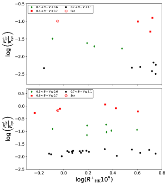
Figure 16: Logarithmic ratio between rotation period and activity cycles over an activity scale given by $\log R_{\rm{HK}}^{+}10^{5}$ and the different colours and symbols distinguish different $B-V$ ranges. Upper panel: Results for the cycles on the long-cycle branch. Lower panel: Results for the cycles on the short-cycle branch.

The correlation between the $\omega_{\rm{cyc}}/\Omega,$ or rather $P_{\rm{rot}}/P_{\rm{cyc}}$ and the Rossby number or the activity index, $R_{\rm{HK}}^{\prime}$, is equivalent to the empirical relation of the form $P_{\rm{cyc}}\propto P_{\rm{rot}}^{\rm{n}}$. On this basis, the ratio of the rotation period and cycle period is

$$\frac{\omega_{\rm{cyc}}}{\Omega} = \frac{P_{\rm{rot}}}{P_{\rm{cyc}}}\propto\frac{1}{P_{\rm{rot}}^{n-1}}.$$ (24)

Therefore, we assume that the activity index $R_{\rm{HK}}^{\prime}$ in the proportionality $\omega_{\rm{cyc}}/\Omega=P_{\rm{rot}}/P_{\rm{cyc}}\propto R_{\rm{HK}}^{\prime}$ (see Eq. 23) is caused by a remaining proportionality of the activity-rotation relation. Thus, we do not expect any dependence between the ratio, $P_{\rm{rot}}^{n}/P_{\rm{cyc}}$, and activity index $R_{\rm{HK}}^{+}$, which we use instead of $R_{\rm{HK}}^{\prime}$ and which is the pure Ca ii H&K flux excess. Consequently, the following applies:

$$\frac{P_{\rm{rot}}^{n^{S}_{i}}}{P_{\rm{cyc}}}(R_{\rm{HK}}^{+}) \propto constant,$$ (25)

and

$$\frac{P_{\rm{rot}}^{n^{L}_{i}}}{P_{\rm{cyc}}}(R_{\rm{HK}}^{+}) \propto constant,$$ (26)

where n is the exponent of the empirical proportionality, the index $S$ and $L$ labelling the two cycle branches, and the index, $i,$ represents different $B-V$ ranges.

To test this assumption, we computed the period ratio (cycle over rotation) as in Eqs. 25 and 26, for both branches, and we used the results obtained in Sects. 5 and 5.4 (see Tables 6 and 8). Figure 16 visualises these results over an activity scale in double-logarithmic figures, colour-coding the $B-V$ ranges. Indeed, here the activity seems to make no difference in any single $B-V$ range, which gives empirical support to the above relation. Yet there are evident differences between different $B-V$ ranges.

Finally, in Fig. 18 we compare the cycle periods from our final empirical relation with a Rossby number

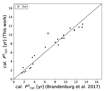
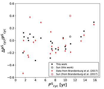
Figure 17: Calculated $P^{S}_{\rm{cyc}}$ obtained from the empirical relation found in this study over the respective values from Brandenburg et al. (2017); the dashed line depicts the identity.

Figure 18: Relative deviation versus cycle on the short-cycle branch for 23 stars contained in both samples; black data points are obtained with our calculated cycle periods, red diamonds from Brandenburg et al. (2017).

with those periods from Brandenburg et al. (2017) for 23 stars located on the short-cycle branch, which are contained in both samples, except HD 103095; this is because the calculated cycle listed in Table 1 is computed with Eq. 14 and the corresponding parameter given in Table 5. This comparison shows a good agreement between both sets of results, except for the Sun.

Comparing the expectations of the 11-year solar cycle given by the empirical relation of Brandenburg et al. (2017) and the one presented here, we find that the estimated solar cycle of 6.6 years by Brandenburg et al. (2017) clearly differs from the observed eleven year solar cycle, while our estimated solar cycle period of 10.3 years is consistent with the 11-year solar cycle. This might be related to our use of smaller $B-V$ ranges, as well as the use of the Rossby number instead of the rotation period. Also, we show the relative deviations of the compared cycles in Fig. 18, and there we can observe a larger scatter of the values obtained by the cycle-activity relation of Brandenburg et al. (2017) than in our final cycle-rotation relation. To quantify this, we computed the corresponding standard deviations of the relative deviations and obtained a standard deviation of 0.22 for the values of the cycle-activity relation of Brandenburg et al. (2017) and a standard deviation of 0.14 for our final cycle-rotation relation.

Furthermore, we performed again a overall F-test (like in Sect. 4.3) to see whether both empirical relations are actually statistically different in a significant way. For the F value, we obtained $F=3.79$, yielding a confidence level of $99.6\%$. Hence, we can assume that the our final cycle-rotation relation is indeed statistically significant in its difference from the one given by Brandenburg et al. (2017), and the reduction of the residual differences of the individual data points is real.

7 Depth of dynamo action

At least some stars in our sample do show two activity cycles: one on the short-cycle branch and one on the long-cycle branch, thus raising the question whether these different activity cycles may be produced by dynamos operating in different depths of the convective zone. A common assumption made by the mean field $\alpha-\Omega$ dynamo theory is that the dynamo action takes place at the bottom of the convection zone. In that case, the relative length scale of the convection could also be seen as representative for the relative depth of dynamo action.

Here, we follow the approach to use the relative depth of the convection zone ($d_{cz}$) instead of the relative length scale of the turbulence ($l/R_{\star}$) as an additional parameter for our cycle relations (see Eqs. 21 and 22). Furthermore, we assume that the constant $a$ in Eqs. 21 & 22 is a scaling factor of the cycle depth. Consequently, we can write

$$\left(\frac{l^{j}_{i}}{R_{\star}}\right) = \frac{d_{cz}}{10^{a^{j}_{i}}},$$ (27)

where index $i$ distinguishes the different $B-V$ ranges and index $j$ is the cycle branch. With this assumption, it is possible to assess the depths where the short and long cycles are produced. Calculating the ratio between the cycle periods located on the long-cycle branch and the short-cycle branch (see Eqs. 21 and 22) and using our assumption on the constant a (see Eq. 27), we express the ratio between the periods on the long- and short-cycle branches as:

$$\frac{P^{L}_{\rm{cyc}}}{P^{S}_{\rm{cyc}}} = \frac{10^{a^{L}_{i}}d_{cz}\tau_{c}Ro^{n^{L}_{i}}}{10^{a^{S}_{i}}d_{cz}\tau_{c}Ro^{n^{S}_{i}}}=\frac{l^{S}_{i}\tau_{c}Ro^{n^{L}_{i}}}{l^{L}_{i}\tau_{c}Ro^{n^{S}_{i}}},$$ (28)

where index $L$ denotes the long-cycle branch and index $S$ is the short-cycle branch, while index $i$ again labels the different $B-V$ ranges. For the cycle-rotation relation on the long-period branch (see Sect 5.4), we assume that the exponent $n$ is the same in both branches, hence $n^{L}_{i}=n^{S}_{i}$. That is supported by our empirical results (see Tables 5 and 7), where the values of $n$ are equal (within the uncertainties) in corresponding $B-V$ ranges.

With this assumption, the terms of $\tau_{c}Ro^{n^{L}_{i}}$ and $\tau_{c}Ro^{n^{S}_{i}}$ cancel each other out, so that the ratio of the cycle periods (see Eq. 28) is reduced to:

$$\frac{P^{L}_{\rm{cyc}}}{P^{S}_{\rm{cyc}}} = \frac{l^{S}_{i}}{l^{L}_{i}}.$$ (29)

Equation 29 shows that the cycle ratio is only proportional to the ratio of the length scale of turbulence $(l)$. Since cycle periods on the long-period branch are – by definition – longer than on the short-cycle branch, the length scale of turbulence $(l)$ must satisfy

$$l^{S}_{i} > l^{L}_{i}.$$ (30)

We therefore conclude that the cycles on the short-cycle period branch are created in layers of the convective zone that are deeper than those where the cycles on the long-cycle branch are produced.

8 Summary and conclusions

In this paper, we revisit the activity cycle-rotation connection for cool main sequence stars with the aim of deriving a universal relation by considering the impact of further stellar parameters, which would be fully consistent with the solar cycle and rotation periods. In particular, we consider the Rossby number as the natural parameter in any such relation, which practically means a ‘normalisation’ of any stellar rotation period by the respective convective turnover time.

Studying the empirical relation between cycle and rotation periods with different approaches, the statistically best empirical description turns out not to be a linear relation – but that of a power law (i.e. linear in the double-logarithmic representation) and an additional $B-V$ dependence must be considered. As suggested by earlier studies, we actually find a bifurcation into a longer and a shorter cycle period branch. For the latter, in this relation, we obtained an average scatter of $\approx$ 20$\%$ among the sample stars.

This scatter can be decreased further by using the Rossby number instead of the rotation period. By considering the convective turnover time as well as the relative depth of the convection zone, we find that the relative deviation between the actual observed and nominal cycle periods decreases to 14$\%$. A further confirmation comes from the Sun, where the calculated cycle length of $10.3^{1.1}_{1.0}$ yr as obtained with our cycle period versus Rossby number relation is fully consistent with the well-known 11-year solar activity cycle.

With the same approach, we also derived a cycle period-Rossby number relation for the long-period branch. Here, we obtained an average scatter of 28$\%$ in the relative deviations, taking the original stellar data against the empirical relation. For the Sun, this branch suggests a (Gleissberg) cycle length of $104^{+50}_{-34}$ yr. This value is on the larger side of the ranges of the suggested Gleissberg cycle periods, which are typically around 90 years, yet given the stellar scatter and its uncertainties, we consider the agreement of our calculated long-period branch with the observed Gleissberg cycle length as satisfactory.

In summary, the solar Schwabe and Gleissberg cycles are reproduced very well in our cycle-Rossby number relation in contrast to the cycle versus rotation representation. In previous studies, the position of the Schwabe cycle in the cycle versus rotation presentation is explained with the assumption of another kind of dynamo, for instance, a transitional dynamo. However, in our study, we have not found any evidence suggesting another kind of dynamo and our approach allows for the interpretation of both the Schwabe and Gleissberg cycles with the same relations that apply to our cool main sequence sample stars on the short- and long-cycle branches. Furthermore, in our sample, we found no objects with a strong deviation in the cycle versus Rossby number relation, which would suggest other dynamos or processes to be at work.

In our study, we also tested whether the cycle period is dependent on the strength of the activity level. For this purpose, we compared the logarithm of the ratio $P_{\rm{rot}}^{n}/P^{S}_{\rm{cyc}}$ with the logarithm of activity index $R_{\rm{HK}}^{+}10^{5}$. By using a power law approach, $P_{\rm{rot}}^{n}$, we avoided a secondary dependency introduced artificially by the rotation–activity relation. Our results suggest that the ratio $P_{\rm{rot}}^{n}/P^{S}_{\rm{cyc}}$ shows no dependence on the activity index $R_{\rm{HK}}^{+}10^{5}$ and, therefore, we conclude that the cycle periods are indeed independent of the activity level, which means there is thus no additional factor in our cycle-rotation or rather cycle-Rossby number relation (in contrast to the aforementioned $B-V$ colour index).

Finally, we briefly discuss indicators for the depth of the respective dynamo operation. In our empirical relation between cycle period and Rossby number, we used the relative depth of the convection zone in place of the relative length scale of the turbulence, which can also be interpreted as a relative depth of the dynamo operation.

From our factor analysis, we found that this relative depth of the convection zone enters with an exponent that is away from unity, which suggests that the dynamo is not created on the bottom the convention zone. However, it should be mentioned here that the derived exponents depend strongly on the other parameters in our relations. Nevertheless, it seems feasible to make an estimation of which cycle type is created in deeper layers. Those located on the short-period branch are probably created by a dynamo operating in deeper layer than those to be associated with cycles located on the long-period branch.

Clearly, the main problem in the entire analysis of the relation between the cycle length and rotation period is the limited number of well known active cycles. Due to this limited number of activity cycles with well-known periods, the derived empirical relations have significant uncertainties. At least the one for stars of solar colour matches the 11-year solar cycle relatively accurately. Still, to verify the solar cycle relation and the other relations, it remains important to find more reliable cycle periods, especially among the long-period cycles. This is a task which requires long-term time series observations. The only way to obtain time series of 30 years and more is to combine observations from different monitoring programs. Hence, Ca II H&K monitoring programs are required to study the cycle-rotation relation, as a larger number of calibration stars exist as well as recipes to ensure consistency between very different instrumentation, epochs, and index definitions.

Finally, we like to comment on the denotation of the two cycle branches as ‘inactive’ and ‘active’, introduced by earlier studies. What is evident is only a bifurcation into short- and long-period branches, as we confirm here for our empirical relations over the Rossby number. Furthermore, our Sun has two activity cycles, where one is located on the ‘inactive’ (short-cycle) branch and one on the ‘active’ (long-cycle) branch. However, we could show that the ratio of $P_{\rm{rot}}^{n}$ and $P_{\rm{cyc}}$ is independent of the strength of activity, including cases where the same star has one cycle on each of those two branches. Hence, we conclude that the bifurcation into those different branches in the diagram of cycle length over rotation period is actually not caused by the activity level of a star, but arises from a difference in depths of dynamo operation in the convection zone, where the respective cycles are created.

In consequence, we think that the hitherto common denotation of the two cycle branches is a misnomer. In Brandenburg et al. (2017), where the co-existing of two activity cycles are investigated, the ‘inactive’ branch was renamed as short-cycle branch and the ‘active’ branch as long-cycle branch. We argue that this denotation of the two branches is better rooted in reality and thus we suggest that the terms introduced by Brandenburg et al. (2017) for the two branches should be used in the future.