SRG/eROSITA X-ray shadowing study of giant molecular clouds

Abstract

Context. SRG/eROSITA is situated in a halo orbit around L2 where the highly variable solar wind charge exchange (SWCX) emission from Earth’s magnetosheath is expected to be negligible. The soft X-ray foreground emissions from the local hot bubble (LHB) and the remaining heliospheric SWCX emissions could be studied in unprecedented detail with eROSITA All-Sky Survey (eRASS) data in a 6-month cadence and better spectral resolution than ROSAT.

Aims. We aim to use eRASS data of the sight lines towards three giant molecular clouds away from the Galactic plane to isolate and study the soft X-ray diffuse foreground emission. These X-ray shadows will serve as calibration baselines for the future three-dimensional structural study of the LHB.

Methods. We conducted spectral analysis on the diffuse X-ray spectra of these clouds from the first four eRASSs to estimate and separate the heliospheric SWCX contribution from the LHB emission.

Results. We find the density of the LHB to be independent of the sight line with $n_{e}\sim 4\times 10^{-3}$ cm^-3, but not the temperature. We report a lower temperature of $kT_{\mathrm{LHB}}=0.084\pm 0.004$ keV towards Chamaeleon II & III (Cha II & III) than Ophiuchus (Oph) and Corona Australis (CrA), in which we measured $0.102\pm 0.006$ and $0.112\pm 0.009$ keV, respectively. We measured the emission measure of the LHB to be $\sim 2\times 10^{-3}\,$cm^-6 pc at medium Galactic latitudes ($|b|\sim 20\degr$). A monotonic increase in the SWCX contribution has been observed since the start of 2020, coincidental with the beginning of solar cycle 25. For Oph, SWCX has dominated the LHB in the $0.3$–$0.7$ keV band intensity since eRASS2. We observed lower SWCX contributions in Cha II & III and CrA, consistent with the expected decreasing solar wind ion density at high heliographic latitudes.

1 Introduction

The notion of the soft X-ray emitting local hot bubble (LHB) emerged after Wisconsin sounding-rocket data showed an anti-correlation between the soft X-ray intensity and neutral hydrogen column density ($N_{\@element{\mathrm{H}}}$) in the southern Galactic hemisphere (Sanders et al. 1977). In their concise yet seminal paper, Sanders et al. (1977) pointed out that the anti-correlation could not be accommodated for by photoelectric absorption but by a displacement effect in which the local volume is filled with an X-ray emitting gas bounded by a thick wall of cool neutral hydrogen gas. In this picture, a low $N_{\@element{\mathrm{H}}}$ (thin) section of the wall is displaced by additional X-ray emitting gas, resulting in a higher X-ray intensity in low $N_{\@element{\mathrm{H}}}$ regions. Independently, Tanaka & Bleeker (1977) reached the same conclusion and coined the term LHB. The existence of the LHB had henceforth become the standard conceptual picture of the local interstellar medium (ISM) — a low H I column density region ($N_{\@element{\mathrm{H}}}\lesssim 10^{20}$ cm^-2) filled with hot plasma extending to $100$–$200$ pc (e.g. see reviews by Bochkarev 1987; McCammon & Sanders 1990; Breitschwerdt 1996). After the launch of ROSAT, shadowing experiments on Draco and MBM12 clouds firmly indicated the presence of a more distant soft X-ray background from the Galaxy in addition to the foreground LHB emission (e.g. Snowden et al. 1991, 1993).

However, ROSAT delivered arguably even more insights into the additional soft emission, which turned out to be foreground emission and led to the discovery of the solar wind charge exchange (SWCX) process. It began with the detection of long-term enhancements (LTEs) in the ROSAT All-Sky Survey (RASS) with durations ranging up to $\sim 8$ hours, which were then found to be correlated with solar wind variations and geomagnetic storms (Freyberg 1994). Later detection of an unexpectedly bright soft X-ray from the Comet C/Hyakutake 1996 B2 with an emission morphology facing the Sun but not the direction of motion strongly suggests that the Sun is the culprit (Lisse et al. 1996). Soon after, Cravens (1997) proposed that the charge exchange process between the cometary neutrals and heavy solar wind ions could explain the comet’s soft X-ray emission. Dennerl et al. (1997) established comets as a class of X-ray sources by systematically searching the archival ROSAT data and they pointed out that the charge exchange between highly charged solar wind ions and cometary neutrals is the dominant emission process. A LTE in the X-ray background was also detected near the outbursts of the comet, prompting Dennerl et al. (1997) and Freyberg (1998) to suggest the Earth could also act as a bright, soft X-ray source from the SWCX process. Concurrently, Cox (1998) pointed out the flowing neutral ISM also provides a source of neutrals to interact with the solar wind. The SWCX emissions from these two sources of neutral atoms are usually referred to as magnetospheric and heliospheric SWCX, respectively (see review by Kuntz 2019).

Distinguishing between the contributions of LHB and SWCX using ROSAT PSPC is challenging due to the reliance on broad-band count rates. Many cross sections of the heavy ions were unknown, further complicating the issue. Before the arrival of more SWCX-focussed missions such as the Diffuse X-rays from the Local Galaxy (DXL), simultaneous modelling of the LHB and SWCX have resulted in sometimes inconsistent results — from estimations of SWCX contributing to half to all of the $\frac{1}{4}$ keV emission in the galactic plane (Koutroumpa et al. 2009; Robertson et al. 2009, and references therein). There was naturally a worry that LHB had become redundant and all the $\frac{1}{4}$ keV emission could be accounted for by SWCX, despite a consistent requirement of additional emission at high galactic latitudes also shown by these studies.

Galeazzi et al. (2014) mostly settled the situation by estimating the heliospheric SWCX contribution in ROSAT using the DXL sounding rocket mission and reported that the LHB still contributes to $\sim 60$% of the emission in the galactic plane. Based on the estimated SWCX contribution from DXL (Galeazzi et al. 2011; Uprety et al. 2016), Liu et al. (2017) measured a LHB temperature of $0.097\pm 0.019$ keV from the ROSAT R2/R1 band ratio map and mapped out the three-dimensional (3D) structure of the LHB assuming a constant electron density plasma. They show that the inferred boundary of the LHB agrees reasonably well with the onset of a higher absorbing column inferred from the local ISM density map (Lallement et al. 2014).

With energy-resolved imaging and repeated all-sky surveys every six months, eROSITA is providing an unprecedented view of the soft X-ray foreground in terms of the depth and differentiation of LHB from SWCX. Situated in a halo orbit around L2, eROSITA is expected to be free of the highly variable SWCX coming from the Earth’s magnetosheath. The energy resolution of $\Delta E\simeq 58$ eV at the C-K line ($0.277$ keV) allows for spectral decomposition of the heliospheric SWCX and LHB components (Predehl et al. 2021), as well as measurements of the properties of the LHB and SWCX intensity in six-month cadence along the chosen sight lines.

In this paper, we study the emissions from three of the darkest X-ray shadows away from the Galactic plane in the German eROSITA sky (Galactic coordinates restricted to $180\degr\leq l\leq 360\degr$, $-90\degr\leq b\leq 90\degr$) — Chamaeleon II & III (Cha II & III), Ophiuchus (Oph), and Corona Australis (CrA). They lie on the boundary of the LHB (Zucker et al. 2022) with accurate distances and are, therefore, ideal calibration points of the LHB properties, which could later be extended to infer the 3D structure of the LHB. Earlier observational work based on ROSAT found the LHB is well described by a single temperature and density plasma (e.g. Liu et al. 2017). We aim to subject this assumption to the tighter constraints set by eROSITA. These sight lines also enable us to infer the time evolution of the relative contribution between the LHB and heliospheric SWCX.

In Sect. 2, we describe the eROSITA observations of the clouds and the specific regions chosen for spectral extraction, as well as the XMM-Newton celestial calibration source as an independent monitoring of the SWCX variation. We lay out the constituents of our spectral model and our spectral fitting procedures in Sect. 3. We report our results and interpretations in Sect. 4. Finally, we deliver our concluding remarks in Sect. 5.

2 Data and calibration

We extracted data of Cha II & III, Oph and CrA from the first four eROSITA All-Sky Surveys (eRASSs). Only data from telescope modules (TM) with on-chip filters (TM 1–4 and 6) were extracted to avoid the light leak issue (Predehl et al. 2021). Four visits to each cloud enable an analysis of the variability over intervals of half a year. The data were processed with the 020 version of the eSASS pipeline (Brunner et al. 2022). Flares were removed using the standard eSASS task flaregti. After removing the flared time intervals, the total vignetting-corrected exposure times within the defined regions (right panel of Figs. 1, 2 and 3) in the first four eRASSs in the $0.2$–$3$ keV band (our spectral-fitting range) are $\sim 760$ s for Cha II & III, $\sim 330$ s for Oph, and $\sim 250$ s for CrA. The difference is mainly caused by their angular distance from the ecliptic poles, where all the great circles of the eROSITA scans merge to result in the maximum exposure time.

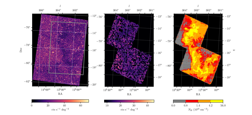
Figure 1: eROSITA 0.2–3 keV image of the shadow cast by Cha II & III. The left panel shows the eROSITA 0.2–3 keV band image of Cha II & III colour-coded with the vignetting-corrected count rate. The grey rectangular box indicates the region shown in the middle and right plots. The middle panel shows the point-source-free region where spectral analysis is carried out. The two rectangular mosaics represent the region covered by the Herschel column density map. The right panel shows the four column density bins that define the regions for spectral extraction. The dotted grid is in the Galactic coordinate system.

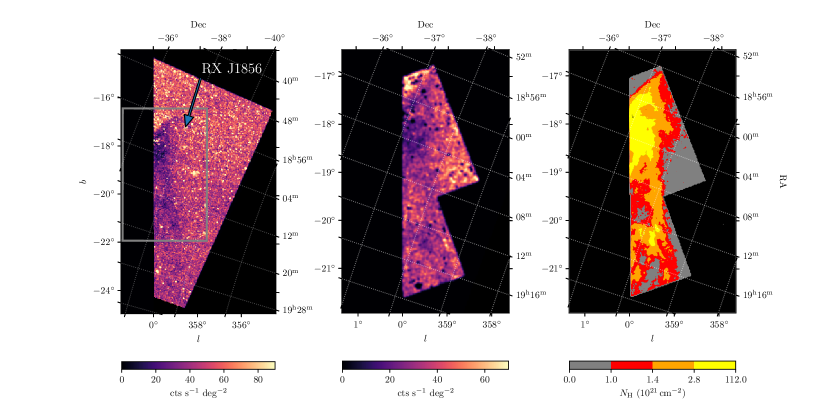
Figure 2: Same as Fig. 1, but for CrA. The dotted grid is in the equatorial coordinate system.

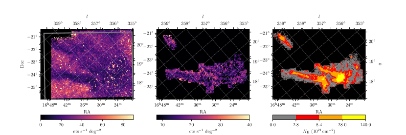
Figure 3: Same as Fig. 1, but for Oph. The dotted grid is in the Galactic coordinate system, with $l$ increasing towards the top left and $b$ increasing towards the top right.

All valid event patterns were used because the low-energy electronic noise component (mostly $\lesssim 0.3$ keV) has been greatly reduced from the 946 (as used in the Early Data Release (Brunner et al. 2022)) to 020 processing version. Thus one could take advantage of more photons to constrain the spectral models at low energies and need not sacrifice higher-pattern events to suppress the electronic noise.

The 0.2–3 keV images of the clouds are shown in the left panels of Figs. 1, 2 and 3. One can observe a clear shadow between $301\degr\lesssim l\lesssim 304\degr$ and $13\degr\lesssim b\lesssim 18\degr$ cast by Cha II & III. The X-ray shadows are even more prominent in the case of CrA and Oph — a consequence of the two clouds being in front of and absorbing the emissions from the bright eROSITA bubbles (Predehl et al. 2020). Point sources were masked using the CheeseMask images produced by the standard eSASS detection chain, as shown in the middle panels.

In our spectral analysis, spectra of varying column density regions were extracted. The extraction regions are colour-coded on the right panels of Figs. 1, 2 and 3 by column density. The hydrogen column density information was obtained from the Herschel Gould Belt Survey Archive (André et al. 2010). The column density maps were produced by fitting the SEDs formed by the 160, 250, 350 and 500 $\mu$m images in a 6″grid at an angular resolution of 18$\aas@@fstack{\prime\prime}$2 (Alves de Oliveira et al. 2014; Bresnahan et al. 2018; Ladjelate et al. 2020). We convolved the column density map to the approximate eROSITA angular resolution of $30$″, then defined four regions bound by the contour levels. Regions of Cha II & III and CrA are defined in this way. Table 2 lists the solid angles of the defined regions.

Cloud	Exposure Time (s)	Region	Area (deg2)	$N_{\mathrm{H}}$ ($10^{21}$ cm-2)
				Herschel	Planck $R$	Planck $\tau_{353}$
		1	1.69	$0.47^{+0.11}_{-0.12}$	$0.75^{+0.14}_{-0.15}$	$0.84^{+0.16}_{-0.19}$
Cha II & III	762	2	2.21	$0.80^{+0.14}_{-0.12}$	$1.01^{+0.11}_{-0.13}$	$1.31^{+0.22}_{-0.18}$
		3	4.14	$1.55^{+0.52}_{-0.33}$	$1.43^{+0.27}_{-0.17}$	$2.36^{+0.67}_{-0.39}$
		4	1.15	$4.10^{+1.02}_{-0.73}$	$2.34^{+0.38}_{-0.28}$	$4.86^{+1.19}_{-0.87}$
		1	1.37	$0.55^{+0.10}_{-0.09}$	$0.60^{+0.11}_{-0.09}$	$0.60^{+0.21}_{-0.15}$
CrA	251	2	1.40	$0.86^{+0.07}_{-0.08}$	$0.89^{+0.12}_{-0.11}$	$1.08^{+0.17}_{-0.19}$
		3	1.32	$1.25^{+0.24}_{-0.14}$	$1.17^{+0.26}_{-0.11}$	$1.64^{+0.34}_{-0.23}$
		4	0.60	$3.54^{+3.09}_{-1.01}$	$2.58^{+1.07}_{-0.55}$	$4.56^{+2.33}_{-1.10}$
		1	3.77	$0.93^{+0.52}_{-0.37}$	$7.86^{+4.66}_{-3.61}$	$4.35^{+1.02}_{-0.77}$
Oph	330	2	2.49	$3.24^{+1.12}_{-1.18}$	$8.69^{+4.41}_{-3.21}$	$5.73^{+1.33}_{-1.05}$
		3	1.40	$8.43^{+2.96}_{-1.90}$	$11.07^{+4.77}_{-3.68}$	$8.41^{+2.44}_{-1.22}$
		4	0.19	$27.89^{+6.56}_{-5.29}$	$38.90^{+20.16}_{-13.44}$	$17.91^{+3.01}_{-3.46}$

Table 1: Summary of the exposure times and the extraction regions in each molecular cloud.

For Ophiuchus, the area coverage of Herschel’s column density map is limited to the cloud core. We extended the area with column density information by using the $\@element[13]{\mathrm{C}}$$\@element{\mathrm{O}}$ 1–0 (110.201 GHz) map observed by the 14 m Five College Radio Astronomy Observatory (FCRAO) telescope (Ridge et al. 2006). This was done by deriving the mean $\@element[13]{\mathrm{C}}$$\@element{\mathrm{O}}$-to-$N_{\mathrm{H}}$ conversion factor from the overlap region of the Herschel and FCRAO maps while taking into account the difference in angular resolution and hence applying this factor to the additional area that the $\@element[13]{\mathrm{CO}}$ map possesses. The result, in the form of the four regions’ contours, is shown in the right panel of Fig. 3.

While the Herschel column density maps provide the exceptional angular resolution necessary for this work, similar to the Planck radiance map ($R$) that also adopts SED fitting to extract $N_{\mathrm{H}}$ information, they are likely to be affected by variations in the radiation field strength caused by increased attenuation of the interstellar radiation field and local heating photons in molecular clouds (Planck Collaboration et al. 2014). Planck Collaboration et al. (2014) suggests the dust opacity at 353 GHz ($\tau_{353}$) is a better tracer of $N_{\mathrm{H}}$ in these regions. To estimate the possible range of $N_{\mathrm{H}}$ in each extraction region, we computed the $N_{\mathrm{H}}$ inferred from the aforementioned tracers and list the results in Table 2.

All the maps were convolved to the common angular resolution of 5′(resolution of the Planck maps) to ensure a fair comparison. The Planck maps were first converted to the corresponding $E(B-V)$ maps using the relations $E(B-V)/R=(5.40\pm 0.09)\times 10^{5}$ and $E(B-V)/\tau_{353}=(1.49\pm 0.03)\times 10^{4}$ using quasars in the diffuse ISM at high Galactic latitudes (Planck Collaboration et al. 2014). Subsequently, we adopted the scaling of $N_{\mathrm{H}}/E(B-V)=4\times 10^{21}$ cm^-2 mag^-1 to get $N_{\mathrm{H}}$ from the $E(B-V)$ maps. This scaling is representative of values derived from the detailed multiphase analysis conducted by Planck Collaboration et al. (2015) and is shown by Lallement et al. (2016) to match the fitted X-ray foreground absorption in 19 XMM-Newton sight lines towards the North Polar Spur.

We note the reasonable agreement between the three tracers, given that there is still a large scatter with each scaling relation we used to convert $R$ and $\tau_{353}$ to $N_{\mathrm{H}}$. The variations of $N_{\mathrm{H}}$ inferred from different tracers inform the scale of systematic uncertainties in our derivation of $N_{\mathrm{H}}$, which is instructive to compare with the best-fit $N_{\mathrm{H}}$ values in Table 2 in Sect. 4. Interestingly, a direct comparison between our best-fit $N_{\mathrm{H}}$ and the values derived from the three tracers would suggest $\tau_{353}$ might be a better $N_{\mathrm{H}}$ tracer towards these high $N_{\mathrm{H}}$ regions, despite the fact that the region boundaries are drawn from the Herschel maps. An exception to the overall agreement is found in region 1 of Oph. The reason for this is likely to be the inaccurate extrapolation of the Herschel map using ¹³CO map when the latter approaches the sensitivity limit in the lowest $N_{\mathrm{H}}$ region.

Background count rates in the $0.3$–$0.7$ keV and $8$-$12$ keV bands of the XMM-Newton routine calibration source RX J1856.5-3754 (RX J1856) were also extracted in order to compare and cross-check our findings on SWCX towards the direction of CrA. The position of RX J1856 relative to CrA is indicated on the left panel of Fig. 2. Appendix A describes the datasets and the results in more detail.

3 Spectral Analysis

This section describes the various components that comprise the soft X-ray spectrum and our spectral fitting procedures. The spectral components are summarised in Fig. 4, which we subsequently elaborate on individually in the rest of the section.

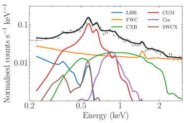
Figure 4: Illustration of all the spectral components taken from Cha II & III.

We divide the physical components into two groups, foreground and background. The former includes the local hot bubble (LHB) and solar wind charge exchange (SWCX) emissions in front of the molecular clouds. The latter comprises the circum-galactic medium (CGM), cosmic X-ray background (CXB) and a Galactic corona (Cor) component (Ponti et al. 2022). The background components, for simplicity, are assumed to be absorbed by the same column within the cloud. In addition, we assume there is no absorption between us and the cloud.

The instrumental background is fixed using the empirical models developed from the filter-wheel closed data accumulated since the launch of SRG. Because the instrumental background differs slightly between the 5 TMs, as shown in Appendix B, the instrumental model used is TM-specific. In Appendix B, we also demonstrate that the eROSITA instrumental background remained stable within the $0.2$–$9$ keV, independent of time and CCD temperature.

3.1 Foreground Components

Chamaeleon II & III are located at a distance of $\sim 190$–$200$ pc (Voirin et al. 2018; Galli et al. 2021) which lie on the surface of the LHB (Zucker et al. 2022). In the simplified scenario, most, if not all, of the soft X-ray photons behind the cloud are absorbed, and one could isolate the foreground soft X-ray emissions due to the LHB and SWCX. As one would see later in Fig. 5 in Sect 4, this is only realised in two regions with the highest column densities, below $\sim 0.4$ keV, where the two foreground components begin to emerge over the CGM emission. The limited energy range where the foreground components dominate but remain below the instrumental background component necessitates using regions (1 and 2) of lower column densities to estimate the contribution of other background components below $\sim 0.4$ keV.

We modelled the LHB as a plasma in collisional ionisation equilibrium (Liu et al. 2017), which is described by the APEC model (Smith et al. 2001). The LHB component is assumed to have solar abundance, given that the Sun is embedded within it. Therefore, the only free parameters of the LHB component are the plasma temperature and the emission measure (EM). We note that for each region, the normalisation of the LHB is scaled by the region area only and remains independent of time (eRASS). The latter reflects that the LHB does not vary on time scales from half a year to two years. As such, the LHB component is only scaled by one free EM parameter, despite different panels showing various combinations of region and eRASS as shown in Fig. 5. This single-parameter component normalisation applies to all other background components (CGM, corona and CXB), and the additional regions introduce no extra free parameter.

The other foreground component is SWCX, which would produce extra diffuse soft X-ray emission in the foreground. The primary source of SWCX in eROSITA is expected to be heliospheric. In heliospheric SWCX, the charge exchange between the neutral atoms in the ISM and ionised particles in the solar wind emits X-ray lines. For magnetospheric SWCX, the solar wind is shocked, compressed, and interacts with the much denser neutral exosphere. The magnetospheric SWCX is expected to vary on a shorter time scale ($\sim$ minutes to days). In eROSITA observations, the magnetospheric SWCX contribution is expected to be negligible (at least for high ecliptic latitude sources) since, being at L2, eROSITA observation geometry intersects only the most tenuous flanks of the magnetosheath. Another potential source of magnetospheric SWCX is the surface of the magnetotail. We believe this effect is minimal because, as shown in more detail in Appendix C, SRG/eROSITA was mostly located outside the magnetosphere due to its halo orbit around L2 during our observations, and additionally, no excess emissions have been found from the frequent observations through the magnetotail of the south ecliptic pole.

The time scale of the heliospheric SWCX is generally longer than the magnetospheric SWCX because the SWCX flux received is integrated along the line of sight up to the edge of the heliosphere, averaging out shorter variations of the solar wind. This is likely true for Cha II & III and CrA that are located at higher ecliptic latitudes ($\beta\sim-62\degr$ and $-14\degr$) and are thus out of the plane of the Parker spiral (Parker 1958). However, the situation is less clear for Oph ($\beta\sim-1\degr$) near the ecliptic plane. A shorter variation time scale in order of hours to days is possible if the sight line is parallel to the pattern of the Parker spiral nearby and vice versa for the perpendicular case (Dennerl et al. in prep).

Ignoring the potential complication for Oph, a simple estimation using the distance to the heliopause ($\sim 120$ AU) and the mean solar wind speed of $450$ km s^-1 yields a time scale of $\sim 460$ days (Kuntz 2019). However, the line-of-sight integration is heavily weighted by the $r^{-2}$-dependence of the solar-wind density away from the Sun, which for reference, is $\sim 1\%$ of its initial density at $r=10$ AU — a distance solar wind only takes $\sim 40$ days to traverse. Therefore, the heliospheric SWCX likely vary from days to weeks. Recently, Qu et al. (2022) showed that the heliospheric SWCX is also correlated positively with the solar cycle using O VII and O VIII line fluxes measured as by XMM-Newton for $10$ years until 2010. Their study revealed a long-term variation in the heliospheric SWCX. However, it is not sensitive to shorter-term variations in the order of or less than half a year, as the width of the line flux bin was chosen to be half a year. SWCX variations on time scales of half a year between CalPV to eRASS3 have also been found by Ponti et al. (2022). In addition, within the $\sim 4$ days scanning time of the eFEDS field, no noticeable variation from SWCX was found (Ponti et al. 2023). The two studies support the expectation that eROSITA is only subject to the heliospheric SWCX observing from L2.

In our spectral fitting, we modelled the SWCX component using the ACX2 (v1.0.3) model (Smith et al. 2012; Foster et al. 2020). The ACX2 model supersedes the older version ACX by including velocity-dependent effects and charge exchange cross sections from the Kronos database (Mullen et al. 2016, 2017; Cumbee et al. 2018). We simplify the model by assuming all the solar wind ions have a single velocity at the mean solar wind speed ($450$ km s^-1), the fraction of neutral Helium at the cosmic value 0.09 (default), solar abundance, recombination type to be single recombination and the acxmodel parameter to be 4. We found the choice of solar wind speed and the acxmodel parameter is not critical to the shape of the SWCX component by inspecting model ACX2 spectra with eROSITA’s spectral resolution, while for the other fixed parameters, we argue that they hold representative values.

The SWCX component is allowed to vary from cloud to cloud primarily because (1) the clouds were observed at different times during eRASSs, and (2) SWCX is expected to be spatially variable on large angular scales. The normalisation of the SWCX component is allowed to vary for each eRASS to account for variability. However, for different regions within the same eRASS, the SWCX normalisation is fixed by the corresponding region area without introducing extra degrees of freedom. Last but not least, we simplify the model on the freeze-in temperature $T_{\mathrm{SWCX}}$. The freeze-in temperature sets the solar wind ion population by assuming the ion population was in collisional ionisation equilibrium with electrons at this temperature. We assume the freeze-in temperature would not change between eRASSs, and therefore, $T_{\mathrm{SWCX}}$ constitutes a single free parameter in the spectra fitting.

3.2 Background Components

We model the non-instrumental X-ray background with three model components: CXB, CGM, and Galactic corona. These components are all modulated by the absorption of the molecular cloud, which we model using the tbabs model (Wilms et al. 2000). It is important to note that we leave $N_{\mathrm{H}}$ as a free parameter and do not impose priors on $N_{\mathrm{H}}$ in all extraction regions, given the systematic uncertainties from various tracers as shown in Table 2. The Herschel $N_{\mathrm{H}}$ information only defines the regions. For simplicity, we take the approximation that all absorptions occur within the cloud, hence the same column density for all background components within the same region.

The presence of the CXB was first observed by Giacconi et al. (1962). The CXB was subsequently found to be isotropic (e.g Schwartz 1980), suggesting an extragalactic origin. Nowadays, it is known that a range of sources, including active galactic nuclei, galaxies, and galaxy clusters, all contribute to the CXB (see Brandt & Yang 2021, for a review). Cappelluti et al. (2017) found that 91% of the observed CXB can be resolved to detected X-ray sources and galaxies from the Chandra COSMOS-legacy field. The CXB spectrum can be modelled as a power law with $\Gamma$ $\sim 1.4$–$1.5$ above $\sim 1$ keV (Vecchi et al. 1999; Kushino et al. 2002; Hickox & Markevitch 2006; Cappelluti et al. 2017). Ponti et al. (2022) also tested a double power law with $\Gamma_{1}=1.9$ below $0.4$ keV, $\Gamma_{2}=1.6$ keV, and $\Gamma_{3}=1.45$ above $1.2$ keV for the CXB component in light of the observational constraints on the CXB (Gilli et al. 2007). While the latter is likely more realistic, we justify using a simple power law with a fixed $\Gamma=1.45$ as most of the CXB is absorbed by the column density of the molecular cloud or subdominant to the CGM component. This value of $\Gamma$ is based on the measurement of Cappelluti et al. (2017), who found $\Gamma=1.45\pm 0.02$. Upon fixing the photon index, the only parameter allowed to vary is the normalisation of the CXB component.

We model the emissions from the Milky Way as a combination of the CGM and Galactic corona, following the treatment of Ponti et al. (2022). The CGM is generally attributed to the hot gas halo of the Milky Way (e.g. Miller et al. 2016; Ponti et al. 2022, and references therein), which could extend up to its virial radius of $\sim 280$ kpc or beyond (Bland-Hawthorn & Gerhard 2016). This hot gas halo could be the shock-heated gas created by accretion onto Milky Way’s dark matter halo (e.g. White & Frenk 1991). In our model, the CGM is assumed to be in collisional ionisation equilibrium like the LHB, but with a much lower abundance of 0.1 $Z_{\odot}$ compared to the conventional value of $Z_{\mathrm{CGM}}=0.3\,Z_{\odot}$. The low abundance is motivated by the finding of Ponti et al. (2022) in the eFEDS field, who found $Z\simeq 0.06\,Z_{\odot}$ with an upper limit of $Z\sim 0.1\,Z_{\odot}$.

The Galactic corona component was detected in the eFEDS field as well and is hypothesised to originate from energetic activities such as supernova explosions with sufficient energies to break free from the Galactic disk and supply hot plasma and metals into the spaces above and below the disk (e.g. Fraternali et al. 2015; Ponti et al. 2022). If one assumes the corona is in collisional ionisation equilibrium with solar abundance, Ponti et al. (2022) inferred a temperature of $\simeq 0.7$ keV. Solar abundance is assumed because the source of the corona is believed to be from chimneys or outflows from the Galactic disk, which are expected to be chemically enriched.

There is a concern that the corona component could be confused with the coronal emission from M dwarfs, as suggested by Wulf et al. (2019). A recent eROSITA study by Magaudda et al. (2020) suggests 65% of the 687 detected M dwarfs have a temperature $\sim 0.5$ keV, similar to the corona component. It is unclear at the moment the significance M dwarfs play in the soft X-ray diffuse emission, whether they are negligible, partly or wholly responsible for the corona component. However, analysing the physical origin of this component is beyond the scope of our work.

With the aforementioned assumptions, only temperatures and their EMs are free to vary in the CGM and corona components. The solar abundances reference for all components modelled by APEC (LHB, CGM, Cor) follows Anders & Grevesse (1989).

3.3 Fitting Procedures

Spectral fitting was performed with the PyXspec software (Arnaud 1996; Gordon & Arnaud 2021). For each cloud, we carried out a simultaneous fit of 80 spectra (5 TMs $\times$ 4 regions $\times$ 4 eRASSs). The spectral fits began with minimising C-statistic (Cash 1979). The resulting covariant matrix would then be used to construct a gaussian proposal distribution in the following Markov Chain Monte Carlo (MCMC) step. We ran three MCMC chains for each cloud using the Goodman-Weare method (Goodman & Weare 2010), each with 100 walkers of 10000 steps. The initial positions of the walkers were randomised to avoid being trapped in local minima, and the first 1000 steps they sampled were discarded. As all the resulting corner plots (marginalised posterior distributions) from merging the three chains exhibit only a single peak without complicated profiles (see Appendix D), we finally constructed the model spectra using the 50 percentile of each parameter (as in Figs. 5, 6 and 7).

4 Results and Discussions

The fit with the highest likelihood for each cloud is shown in Figs. 5, 6 and 7 with the corresponding parameters in Table 2. Figs. 5, 6 and 7 are arranged such that each row corresponds to the observation within the one eRASS, as indicated on the right axis. Each column corresponds to spectra extracted within the same region, as defined by the $N_{\mathrm{H}}$ maps as shown in the right panel of Figs. 1, 2 and 3. Column density increases from left to right. We present the spectral fit in this manner so that the difference between the rows reflects the variations from SWCX, and the difference between the columns shows the absorption of the background components. There are no strong correlations between the parameters, as evidenced by the two-dimensional projections of the posterior distributions shown in Appendix D.

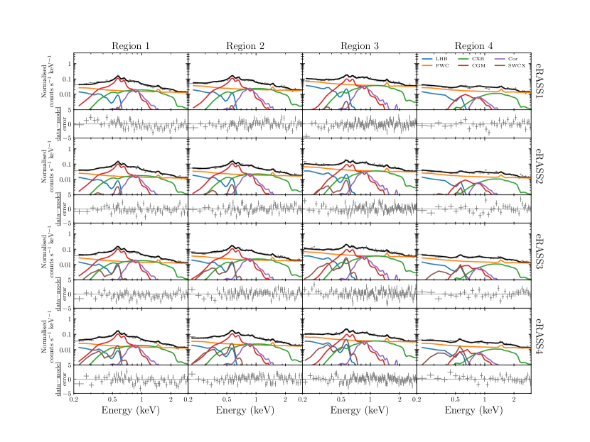
Figure 5: Spectral model of Cha II & III as functions of time in half-year intervals (from top to bottom row) and column density (from left to right column). Each panel shows the TM-averaged data in grey and the corresponding model in black. The constituents of the models are also shown (see the legend).

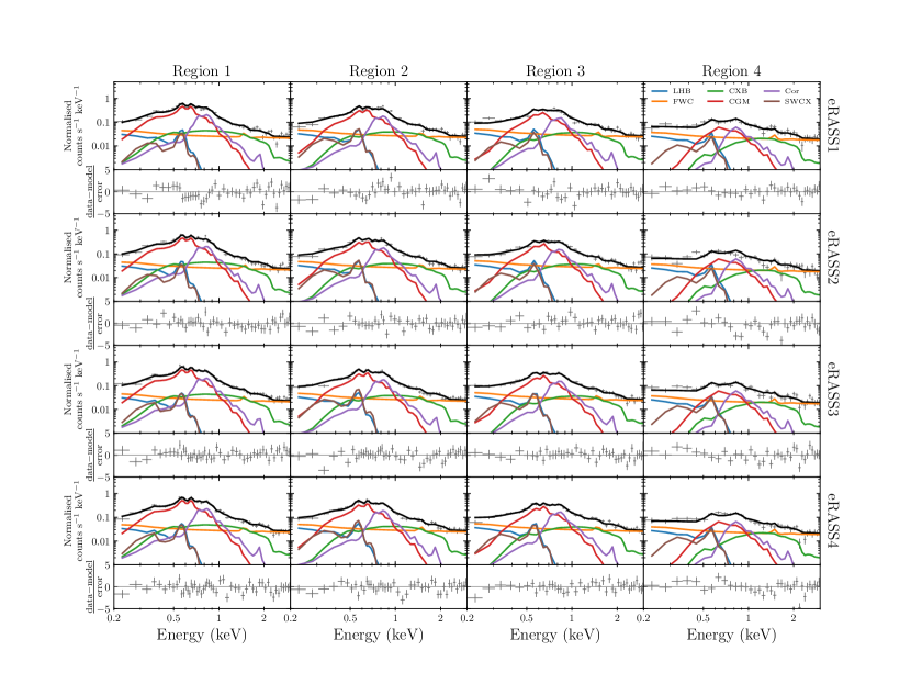
Figure 6: Same as Fig. 5, but for CrA.

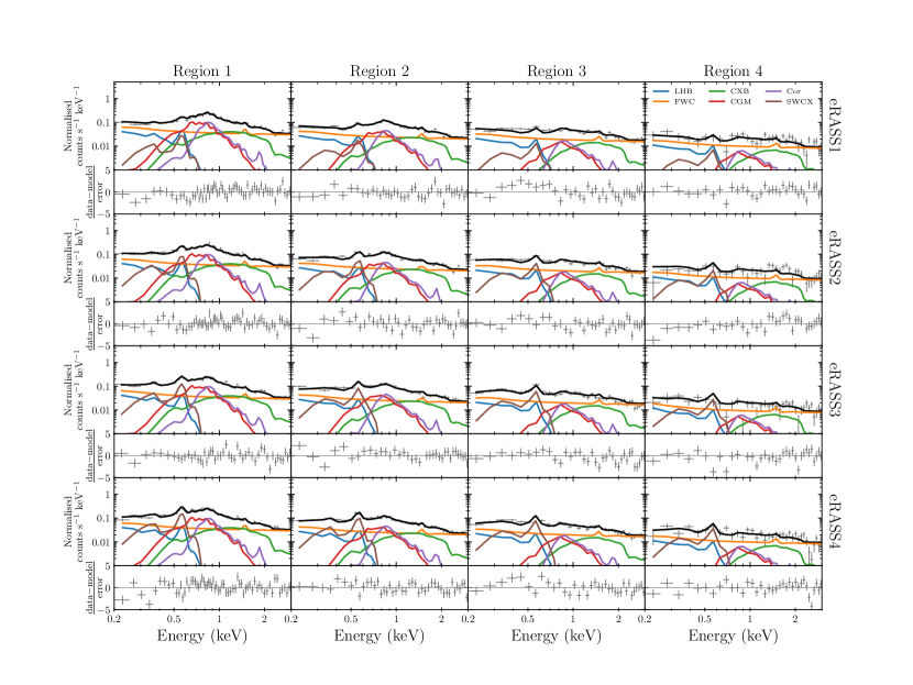
Figure 7: Same as Figs. 5 and 6, but for Oph.

Table 2: Fit parameters of the spectral fitting.

Cloud	Cha II & III	Oph	CrA
$kT_{\mathrm{LHB}}$	$0.084^{+0.004}_{-0.004}$	$0.102^{+0.006}_{-0.006}$	$0.115^{+0.012}_{-0.011}$
$\mathrm{EM}_{\mathrm{LHB}}$	$2.563^{+0.356}_{-0.299}$	$2.062^{+0.237}_{-0.221}$	$1.913^{+0.369}_{-0.284}$
$kT_{\mathrm{SWCX}}$	$0.109^{+0.003}_{-0.004}$	$0.110^{+0.002}_{-0.002}$	$0.108^{+0.005}_{-0.006}$
$n_{\mathrm{SWCX,e1}}$	$0.192^{+0.217}_{-0.159}$	$1.687^{+0.511}_{-0.530}$	$3.215^{+1.297}_{-1.182}$
$n_{\mathrm{SWCX,e2}}$	$0.495^{+0.306}_{-0.230}$	$4.948^{+0.616}_{-0.617}$	$3.271^{+1.207}_{-1.177}$
$n_{\mathrm{SWCX,e3}}$	$1.544^{+0.428}_{-0.305}$	$7.214^{+0.783}_{-0.811}$	$4.200^{+1.235}_{-1.102}$
$n_{\mathrm{SWCX,e4}}$	$2.596^{+0.540}_{-0.426}$	$8.635^{+0.915}_{-0.834}$	$3.973^{+1.110}_{-1.232}$
$N_{\mathrm{H,reg1}}$	$1.106^{+0.062}_{-0.059}$	$2.618^{+0.191}_{-0.162}$	$0.641^{+0.050}_{-0.044}$
$N_{\mathrm{H,reg2}}$	$1.434^{+0.066}_{-0.054}$	$3.665^{+0.191}_{-0.177}$	$1.196^{+0.063}_{-0.052}$
$N_{\mathrm{H,reg3}}$	$2.313^{+0.070}_{-0.058}$	$5.566^{+0.215}_{-0.220}$	$1.673^{+0.067}_{-0.062}$
$N_{\mathrm{H,reg4}}$	$4.258^{+0.124}_{-0.085}$	$6.582^{+0.415}_{-0.370}$	$3.324^{+0.118}_{-0.113}$
$kT_{\mathrm{CGM}}$	$0.183^{+0.002}_{-0.002}$	$0.270^{+0.010}_{-0.011}$	$0.213^{+0.005}_{-0.005}$
$\mathrm{EM}_{\mathrm{CGM}}$	$6.950^{+0.437}_{-0.478}$	$5.581^{+0.851}_{-0.745}$	$12.529^{+0.799}_{-0.673}$
$kT_{\mathrm{Cor}}$	$0.746^{+0.017}_{-0.014}$	$0.719^{+0.017}_{-0.018}$	$0.613^{+0.014}_{-0.015}$
$\mathrm{EM}_{\mathrm{Cor}}$	$0.670^{+0.034}_{-0.039}$	$2.294^{+0.222}_{-0.226}$	$3.272^{+0.211}_{-0.226}$
$\mathrm{norm}_{\mathrm{CXB}}$	$0.237^{+0.003}_{-0.003}$	$0.286^{+0.006}_{-0.007}$	$0.278^{+0.008}_{-0.008}$

4.1 SWCX

For Cha II & III, one can immediately identify the monotonically increasing SWCX component from eRASS1 to eRASS4, in line with the observations in eFEDS and eRASSs (Ponti et al. 2022, Dennerl et al. in prep.). The SWCX contribution is negligible in eRASS1, matches the O VII line from the LHB subsequently at eRASS3, then ultimately dominates the foreground O VII emission in eRASS4. This trend echoes the natural expectation and the findings by Qu et al. (2022), where the heliospheric SWCX is positively correlated with the solar cycle (solar cycle 25 began on December 2019, as well as eRASS1).

We found the best-fit $kT_{\mathrm{SWCX}}\sim 0.1$ keV for all three sight lines, a value consistent with solar wind data (von Steiger et al. 2000; Gloeckler & Geiss 2007). Despite similar temperatures of the LHB and SWCX ($kT_{\mathrm{LHB}}\simeq kT_{\mathrm{SWCX}}\simeq 0.1$ keV), the spectral shapes of the SWCX and LHB are significantly different — SWCX has two prominent peaks, C VI at $0.37$ keV and O VII at $0.57$ keV, while the LHB has both of these prominent emission lines, an extra rising continuum towards the low energy from radiative recombination and bremsstrahlung is present. Combining such difference with the fact that only the SWCX component is allowed to vary between eRASSs, eliminates much of the degeneracy between the two components, given our SWCX spectral model is correct and our constant $kT_{\mathrm{SWCX}}$ assumption is valid. The (lack of) correlations between the LHB and SWCX parameters can be shown from the posterior distributions of the model parameters in Fig 14.

Fig. 8 summarises the SWCX variability to the directions of the three clouds. It shows the 0.3–0.7 keV band intensities from the models as a function of eRASS. This energy band includes most of the emissions from our SWCX component. Clear increasing trends are observed for all the clouds, showing the correlation with the solar activity irrespective of the pointing direction. Interestingly, among the three clouds, we observe that the SWCX intensity is the highest towards Oph and the lowest towards Cha II & III. We argue this is likely the difference in the zero-level SWCX, caused by the difference in the solar wind density, which is a decreasing function of heliolatitude (e.g. see Fig. 18 of Porowski et al. 2022). Ignoring the minor difference between heliolatitude and ecliptic latitude ($\beta$), one could see this argument matches, at least qualitatively, with the ecliptic latitude of the clouds — Cha II & III has the highest $\beta\sim-62\degr$, followed by CrA at $\beta\sim-14\degr$, and finally Oph at $\beta\sim-1\degr$. As a result, the LHB intensity dominates the SWCX emissions from Cha II & III in all eRASSs in this band, but SWCX overtook it towards Oph since eRASS2.

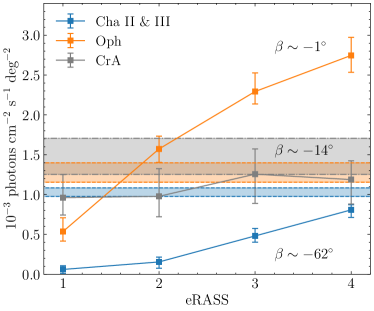
Figure 8: Variation of the model SWCX intensity in the 0.3–0.7 keV band in eRASS1–4. The LHB intensities within $1\,\sigma$ confidence level in the same band are also shown by the shaded regions.

We notice that the rate of increase of SWCX intensity is not at all constant and differs from cloud to cloud. Explaining the precise trends is complex and is beyond the scope of this work. To complicate the issue further, we point out that Fig. 8 contains a caveat where the observations of different clouds made within the same eRASS were not done simultaneously. Instead, they could differ up to $\sim 1.5$ months in the case of CrA ($\lambda\sim 282\degr$) and Cha II & III ($\lambda\sim 246\degr$), because eROSITA’s scanning approximately follows the ecliptic longitude ($\lambda$) with a progression of about 1°per day.

The background $0.3$–$0.7$ keV count rate of RX J1856 located in the neighbourhood of CrA indicates a similar trend as CrA from eRASS1–3 (see Table 7). This comparison suggests our inferred SWCX contribution from spectral fitting is reliable, and indeed the increase in SWCX emission from CrA is less pronounced than the rest (see Appendix A for more discussion).

4.2 LHB

We found the temperature of the LHB to range from $0.084^{+0.004}_{-0.004}$–$0.115^{+0.012}_{-0.011}$ keV from the three sight lines. We also found EM_LHB to span a range from $1.91^{+0.37}_{-0.28}$ – $2.56^{+0.36}_{-0.30}\times 10^{-3}$ cm^-6 pc. As mentioned in Bluem et al. (2022), a direct comparison of these values, which are derived from the APEC model in AtomDB version 3.0.9, with those measured by Liu et al. (2017) is no longer valid due to the updates introduced since its publication date. Therefore, we repeat the same spectral fitting using AtomDB version 3.0.3, released about half a year before the publication of Liu et al. (2017). This result is shown in more detail in Appendix E. In summary, the LHB temperature we found is consistent with the SWCX-subtracted measurement from ROSAT by Liu et al. (2017), who found $kT_{\mathrm{LHB}}=0.097\pm 0.019$ keV averaging across the whole sky. In terms of EM, our measurement is in line with values inferred from the EM map of Liu et al. (2017). One could also compare our LHB measurement to McCammon et al. (2002), who observed the diffuse X-ray background using microcalorimeters with a high energy resolution of $5$–$12$ eV on a sounding rocket. McCammon et al. (2002) reported a $kT_{\mathrm{LHB}}$ of $0.099$ keV and an $\mathrm{EM}_{\mathrm{LHB}}$ of $8.8\times 10^{-3}$ cm^-6 pc — a similar temperature but a significantly different $\mathrm{EM}_{\mathrm{LHB}}$. The main sources of the discrepancy are likely to be a higher Galactic latitude in their observations ($|\Delta b|\sim 40\degr$), a limited knowledge of SWCX at the time, which was not modelled, as well as a significantly fainter Galactic halo component ($\mathrm{EM}_{\mathrm{CGM}}=3.7\times 10^{-3}\,$cm^-6 pc) in their spectral fits.

Using the Wisconsin B/C band intensity ratio, Snowden et al. (1990) reported a dominantly longitudinal LHB temperature dipole, from $10^{5.9}$ K towards the Galactic anti-centre to $10^{6.2}$ K towards the Galactic centre. Later, the existence of the temperature dipole was further consolidated using X-ray shadows and their ROSAT R2/R1 band ratio by Snowden et al. (2000), which show a minimum temperature of $10^{6.04}$ K ($0.09$ keV) near the Galactic anti-centre and a maximum of $10^{6.13}$ K ($0.11$ keV) at the Galactic centre. We observe the same trend and systematic temperature variation in the three molecular clouds, which shows a decreasing temperature from $0.084^{+0.004}_{-0.004}$ keV at $l\sim 300\degr$ to $0.115^{+0.012}_{-0.011}$ keV at $l\sim 360\degr$, although the X-ray shadows in Snowden et al. (2000) are located at higher latitudes ($|b|\gtrsim 20\degr$). We would like to note it is not clear whether this is a real temperature change, as incorrect modelling of the absorption could also result in an apparent temperature change in the LHB.

It is also interesting to test if the LHB is homogeneous in density with known distances of the clouds in literature. The distances to these clouds were mainly derived from Gaia-DR2 astrometry of young stars embedded within the cloud complexes. For instance, the distances to Cha II & III are known to a very high accuracy from Gaia parallax measurements — Cha II is $197.5^{+1.0}_{-0.9}$ pc away (Galli et al. 2021) and Cha III $199^{+20}_{-18}$ pc (Voirin et al. 2018). One could infer the electron density $n_{e}$ of the LHB using

$$\mathrm{EM} = \int^{L}_{0}n_{e}(l)n_{\@element{\mathrm{H}}}(l)dl,$$ (1)

where $n_{\@element{\mathrm{H}}}$ is the hydrogen density and $L$ is the distance to the molecular cloud concerned. We simplify the expression further by adopting a few assumptions — the LHB is completely volume-filling up to the clouds with a constant density and it is fully ionised with $n_{\@element{\mathrm{He}}}$/$n_{\@element{\mathrm{H}}}=0.1$, so that the electron density is $1.2$ times the hydrogen density $n_{\@element{\mathrm{H}}}$ of the LHB plasma (Snowden et al. 2014). Therefore, we have

$$n_{e}=\sqrt{\frac{1.2\mathrm{EM}}{L}}.$$ (2)

We assume further that the distance to both cloud complexes is $L\simeq 198$ pc with negligible uncertainty compared to the EM, we infer $n_{e}=3.94^{+0.26}_{-0.24}\times 10^{-3}\leavevmode\nobreak\ \mathrm{cm}^{-3}$. This dwells on the low side, but is nonetheless consistent with the measurement of $n_{e}=(4.68\pm 0.47)\times 10^{-3}$ cm^-3 by Snowden et al. (2014). Similarly, we estimate the electron density of CrA and Oph using the calculation above using their most recent distance measurements and present the results in Table 3.

Cloud	Distance (pc)	$n_{e}$ ($10^{-3}$ cm-3)	$P_{T}/k$ ($\mathrm{cm^{-3}\,K}$)	Distance references
Cha II & III	$197.5^{+1.0}_{-0.9}$ & $199^{+20}_{-18}$	$3.94^{+0.26}_{-0.24}$	$7380^{+860}_{-780}$	1, 2
Oph	$141.2^{+8.4}_{-7.5}$	$4.19^{+0.23}_{-0.23}$	$9520^{+1110}_{-1050}$	3
CrA	$149.4^{+0.4}_{-0.4}$	$3.92^{+0.36}_{-0.30}$	$10050^{+2070}_{-1660}$	4

Table 3: Distances to the clouds and the estimation of the LHB electron density and thermal pressure along these sight lines.

(1) Galli et al. (2021); (2) Voirin et al. (2018); (3) Cánovas et al. (2019); (4) Galli et al. (2020)

With the conversion from EM to electron density, we present the posterior distributions of the LHB properties in Fig. 9. Despite the three lines of sight agreement on the LHB density at $\sim 4\times 10^{-3}$ cm^-3, the LHB temperature inferred from Cha II & III is significantly colder than the rest. The LHB properties towards Oph and CrA agree at $1\,\sigma$ level but differ from those derived from Cha II & III at $\geq 3\,\sigma$ level. The variation in electron density of the three lines of sight is a constant within $10$%.

We would like to highlight that the three chosen sight lines of significantly different distances (Cha II & III is $\sim 40\%$ farther than the rest) corroborate a single LHB density within $10$% is an interesting result. This result strongly indicates that the LHB extends up to the molecular clouds’ distance unless the LHB density or the volume filling factor is much more variable than we assumed.

The presence of a temperature gradient is not completely surprising as magneto-hydrodynamic (MHD) simulations have already shown the turbulent temperature and density structures sustained by supernova explosions in the ISM (e.g. see Fig. 1 of Hill et al. 2012, de Avillez & Breitschwerdt 2005). It is reasonable to find varying temperature densities when integrating the emission in the turbulent LHB medium along different lines of sight. The fact that we inferred consistent LHB properties from Oph and CrA, which are separated by a significant angular separation of $\sim 35$°, indicates the constant temperature and density assumption is a reasonable modelling simplification to the more complicated scenario presented by MHD simulations.

We estimate the thermal pressure inside the LHB along the three lines of sight following the treatment in Snowden et al. (2014) using

$$P_{T}/k=nT\simeq 1.92n_{e}T,$$ (3)

where $k$ is the Boltzmann constant and $n$ is the total particle density. We found $P_{T}/k$ to be in the range of $6600$–$12100\,\mathrm{cm^{-3}\,K}$ (see Table 3). The resulting pressures are consistent with a constant, unlike the plasma temperature, as a result of propagating the uncertainties of $n_{e}$ and $T$. However, we note that there is a hint of pressure inhomogeneity between Cha II & III and the other two clouds ($\sim 1\,\sigma$), which could indicate a recent supernova or stellar wind expanding from within the LHB that has not yet attained pressure equilibrium with the ambient medium.

The LHB is more elongated in the direction perpendicular to than along the Galactic plane, most probably due to the higher pressure exerted by the ISM in the Galactic disk (Liu et al. 2017). If the LHB is expanding adiabatically, we would expect a lower pressure also towards the Galactic poles. Unfortunately, our current samples cannot probe the Galactic-latitudinal dependence comprehensively as they are close to the Galactic plane and are only valid within $13\degr\lesssim|b|\lesssim 22\degr$.

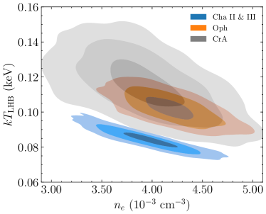
Figure 9: Posterior distributions of the temperature and electron density of the LHB. The contours indicate the 1, 2 and 3 $\sigma$ confidence levels (enclose $\sim$ 39, 86 and 99% of the probability from the highest density).

4.3 Background Components

As we are probing the regions with some of the highest column density away from the Galactic plane, naturally, our analysis is not the best suited to the analysis of the background components located beyond $\sim 200$ pc from us. Nonetheless, even from the images (left panels of Figs. 1, 2 and 3), one could see the emissions from the eROSITA bubbles would bias our conclusion about the background components. Therefore, we begin our discussion with Cha II & III, the only cloud in our samples not located in front of the eROSITA bubbles, hopefully giving more reliable results.

It is instructive to begin by comparing the normalisation of the isotropic CXB component with literature values. With a single power-law with $\Gamma=1.48$, Chen et al. (1997) found $\mathrm{norm}_{\mathrm{CXB}}=10.5\pm 0.4$ photons cm^-2 s^-1 sr^-1 at 1 keV, corresponding to $(3.2\pm 0.2)\times 10^{-3}$ photons cm^-2 s^-1 deg^-2, using a combination of ROSAT and ASCA. More recently, Cappelluti et al. (2017) found $\mathrm{norm}_{\mathrm{CXB}}=(3.32\pm 0.05)\times 10^{-3}$ photons cm^-2 s^-1 deg^-1 at 1 keV from the much more sensitive $2.15\,\mathrm{deg}^{2}$ Chandra COSMOS-legacy field data. Upon removing all the X-ray detected sources, they found $\mathrm{norm}_{\mathrm{CXB}}$ drops to $(1.27\pm 0.08)\times 10^{-3}$ photons cm^-2 s^-1 deg^-1 at 1 keV, corresponding to a decrease of $\sim 2.5$ times. Our measurement of $\mathrm{norm}_{\mathrm{CXB}}$ for Cha II & III, but also the other two clouds, fall between the values of Cappelluti et al. (2017) before and after the X-ray detected source removal. This is expected as eROSITA is much less sensitive and has a lower angular resolution than Chandra’s 4.6 Ms COSMOS-Legacy survey, naturally detecting much less detected X-ray sources to exclude in our analysis.

We found the CGM component to be similar in temperature and EM as the value inferred from the eFEDS field (Ponti et al. 2022), despite the completely different line-of-sight. The eFEDS field and Cha II & III are separated by $\sim 85\degr$ in different galactic hemispheres and latitudes so that it could be a glimpse of an approximately spherical Milky Way hot halo preferred by the analysis of Bregman et al. (2018), but it is certainly far from conclusive. Similarity can also be found in the temperature of the corona component ($\sim 0.7$ keV) when compared with the thermal equilibrium model in Ponti et al. (2022). However, we found a EM_Cor that is higher than the eFEDS field (EM${}_{\mathrm{eFEDS}}=(0.385\pm{0.025})\times 10^{-3}\,\mathrm{cm}^{-6}\,\mathrm{pc}$). This is qualitatively consistent with the picture that the corona is more confined to the Galactic plane from outflows from supernovae or stellar winds since Cha II & III has a lower galactic latitude than the eFEDS field ($|b|\sim 30\degr$).

A high galactic latitude ($|b|>30\degr$) HaloSat study by Bluem et al. (2022) also detected the corona component, in which they call the hot component of the CGM, to have the same temperature $kT_{\mathrm{Cor}}\sim 0.7$ keV. They inferred the same temperature for the cooler CGM component ($kT_{\mathrm{CGM}}\sim 0.18$ keV) as our Cha II & III sight line. However, our assumptions of the abundances differ — both their cool and hot CGM components are assumed to have $Z=0.3\,Z_{\odot}$. Regarding the EM, our values of both CGM and corona are significantly higher than those found by Bluem et al. (2022) in the closest sight lines (separated $\sim 15\degr$ from Cha II & III along the galactic longitude). The reason for the discrepancy is not apparent except for the different assumed abundance of both components. One possible explanation could be that the corona component is flattened along the Galactic plane, so the path length through a flattened corona increases more significantly towards the Galactic plane, resulting in a steep increase in EM.

For Oph and CrA, which are situated in front of the eROSITA bubbles, one could easily observe their spectra are much more enhanced around $\sim 0.8$–$1$ keV, where the Ne IX, Ne X and various $\@element{\mathrm{Fe}}$ lines are. The enhancement is most certainly coming from the eROSITA bubbles, which causes the EM of the corona component to $3$–$5$ times the value in Cha II & III. Naturally, the bubbles affect not only the fit to the corona component but also the CGM component, as their spectra largely overlap. The CGM is hotter towards Oph, while a much brighter but cooler CGM is preferred towards CrA. There are at least two possibilities that could contribute to the difference: (1) Oph has a higher column density in general, which could bias towards a higher CGM temperature because the temperature proxy O VIII/O VII line ratio could also be accommodated for by a higher column density; (2) the properties of the northern and southern eROSITA bubbles are different, where the northern bubble is likely hotter. The second possibility can be explored and constrained relatively tightly with large regions within the northern and southern eROSITA bubbles at much lower column densities, which would largely remove the ambiguity caused by significant opacity. Nevertheless, the eROSITA bubbles are not expected to affect the measured properties of the foreground components because of the high absorption.

5 Summary and Conclusions

We performed X-ray shadowing experiments on three giant molecular clouds using the data from the first four eRASSs. eROSITA spectra of the clouds allow us to separate the heliospheric SWCX and LHB contributions in soft X-ray foreground emission. We observed a monotonic increase of SWCX since eRASS1, independent of the cloud, matching the expectation based on the solar cycle. An ecliptic latitudinal dependence is also observed, consistent with the expected decreasing solar wind ion density.

From the known distance to the clouds, we found a constant electron density of the LHB plasma towards all three clouds, with $n_{e}\sim 4\times 10^{-3}$ cm^-3. However, we measured a lower LHB temperature towards Cha II & III ($kT_{\mathrm{LHB}}=0.084^{+0.004}_{-0.004}$ keV) compared to Oph and CrA ($\simeq 0.1$ keV). Our results show for the first time that there is a possible galactic longitudinal, but not a latitudinal gradient in the LHB temperature after the subtraction of SWCX. We also found that the thermal pressure in the LHB is consistent with constant given the current measurement uncertainty.

Appendix A Cross-checking the SWCX variation with XMM-Newton’s routine calibration source RX J1856.5-3754

We would like to have an indicator of SWCX variability independent of our spectral analysis. Therefore, we used the EPIC-MOS2 data on board XMM-Newton of the routine calibration source RX J1856.5-3754 (hereafter RX J1856). RX J1856 is a neutron star revisited by XMM-Newton approximately every six months for calibration. For the four observations carried out during the eRASSs, each has an exposure time ranging from $71500$–$74600$ s. These observations provide an independent constraint on the SWCX level because of its proximity to CrA, as indicated by the left panel of Fig. 2 with ($l$,$b$) = ($358\aas@@fstack{\circ}59962$, $-17\aas@@fstack{\circ}21311$). Both eROSITA and XMM-Newton require the solar angle to stay within $90\pm 20$°, owing to operational considerations such as ensuring a sufficient power supply from the solar panels and thermal stability. Therefore, the close spatial proximity of two celestial sources would also entail a close temporal coverage by eROSITA and XMM-Newton.

To infer SWCX variation, we focus on the background region count rate during each visit instead of the neutron star itself. MOS2 is a natural choice; all six outer ring CCDs remained operational despite being configured to the small window mode. On the other hand, two of the outer ring CCDs of MOS1 were lost due to micrometeoroid impacts, decreasing the background area. EPIC-pn was configured to the small window mode; therefore, it does not provide sufficient background region for analysis.

We found the count rates were high at the beginning of all four visits due to the radiation belts. These periods were removed. We note that XMM-Newton observations are affected not just by heliospheric SWCX but also by magnetospheric SWCX. We attempt to minimise the contribution from the latter, at least the time-variable component (variable in a time scale of hours, see Kuntz (2019)) of it, by filtering flares in the softer band ($0.3$–$0.7$ keV) within the comparatively long ($\gtrsim 20$ h) exposure time in each visit. We found no flares in the first two visits, and $\sim 8\%$ of exposure times were discarded in the third visit from the filtering. Unfortunately, the fourth visit on 11 October 2021 suffered from an enhanced quiescent background which cannot be cleaned. Further investigation into the radiation levels from all the instruments on board XMM-Newton reveals that a coronal mass ejection likely caused this. eROSITA also suffered from an enhanced background during this period; however, we could identify and remove this period from the data because of the much more extended coverage. Moreover, CCD5 of MOS2 were in an anomalous state at least during the first and third visits, where the background below 1 keV was strongly enhanced (Kuntz & Snowden 2008). To err on the safe side, we removed CCD5 in all visits from the analysis.

From the sight line of CrA, we found the least increase in SWCX from eRASS1–4. Models with a constant SWCX could also fit the eRASS1–4 data, considering the measurement uncertainties. Nonetheless, we calculate the background count rates from the RX J1856 datasets to inspect the match. We report count rates from two bands — $0.3$–$0.7$ keV for variation in SWCX and $8$–$12$ keV for instrumental and particle background monitoring. The count rates and the eROSITA and XMM-Newton coverage period, are listed in Table 7.

eROSITA Coverage	XMM-Newton Coverage	$0.3$–$0.7$ keV	$8$–$12$ keV
2020-Apr-10–2020-Apr-14	2020-Mar-31–2020-Apr-01	$5.989\pm 0.045$	$2.244\pm 0.019$
2020-Oct-13–2020-Oct-17	2020-Sep-15–2020-Sep-16	$6.123\pm 0.048$	$2.286\pm 0.020$
2021-Apr-08–2021-Apr-14	2021-Apr-01–2021-Apr-02	$6.101\pm 0.046$	$2.270\pm 0.019$
2021-Oct-12–2021-Oct-17	2021-Oct-11–2021-Oct-12	$7.934\pm 0.062$	$2.976\pm 0.025$

Table 4: Background count rate of the field of RX J1856.5-3754 as observed by XMM-Newton/EPIC-MOS2 in a similar time period of eROSITA’s coverage of CrA.

The 0.3–0.7 keV count rates appear to be constant from the period corresponding to eRASS1–3. While the increase from eRASS1 to eRASS2 appears to be $\gtrsim 1\,\sigma$ significance at first glance, but coincidentally the instrumental or particle background was also enhanced as evidenced by the 8–12 keV band, which could likely cause the enhancement. We cannot attribute any count rate increase in eRASS4 to SWCX because of the coronal mass ejection that raised the count rates significantly in both bands (see Sect. 2). In summary, the SWCX variation observed by XMM-Newton in approximately the same epoch as the first three eRASSs seems to agree with eROSITA, which was relatively constant in time towards CrA, despite the uncertainty in determining the magnetospheric SWCX level.

Appendix B Filter wheel closed data in 020 processing version

To study low-intensity diffuse emission, one needs to separate the contribution of the eROSITA instrumental background of the total measured intensity. The most direct way to estimate the instrumental background is by measuring the background level when the filter wheel is rotated to the CLOSED position. For the study of the local hot bubble (LHB) assuming the canonical plasma temperature of $0.1$ keV, the relevant energy range for spectral analysis is $\lesssim 0.6$ keV. The emission of the LHB is expected to dominate the overall X-ray background at an even lower energy ($<0.2$ keV) so that spectral analysis in this range would permit more stringent constraints to the properties of the LHB plasma. However, the lack of effective area combined with the rapidly increasing instrumental background of eROSITA $\lesssim 0.2$ keV makes this impossible. Therefore, the useful spectral range to constrain the LHB is limited to $0.2<E\lesssim 0.6\,\mathrm{keV}$. The main sources of instrumental background at this energy range include electronic noise arising from the circuitry and secondary X-rays created by high-energy particles hitting the camera (Freyberg et al. 2020). The background induced by high-energy particles, commonly referred to as the particle background, does not dominate in the energy range concerned. The particle background dominates the spectrum at $E>4$ keV in the case of eROSITA. Due to an update of the pipeline processing of eROSITA data since version 010 (also implemented in the newer version 020), which includes improvements to the pattern identification algorithms to suppress the electronic noise at the low energy end, the instrumental background also changes accordingly. In this section, we present the filter-wheel-closed (FWC) data in the latest 020 version at the time of writing and their extraction procedures.

The 020 processing version provides the broadest uniformly calibrated eROSITA dataset thus far, in the sense that all retrieved eROSITA event lists, from the CalPV phase to the completion of eRASS4 of all 7 TMs have been processed. Despite the pipeline processing improvements, its breadth supersedes the 010 version in terms of temporal coverage where only the data prior to eRASS2 were processed. The temporal coverage in the even earlier 946 processing version was similar to 020. However in contrast to 020, TM4 data were not processed after a micro-meteoroid hit the detector on 23 February 2020 (Freyberg et al. 2022). For this reason, we had fewer signals for spectral analysis when using the 946 dataset. Complete temporal coverage from eRASS1 to eRASS4 of all the TMs (only TM1-4 and 6 were used for analysis due to optical light leak in TM5 and 7 (Predehl et al. 2021)) allows us to have a better estimation of the contamination introduced by the time-variable SWCX component.

Filter-wheel-closed spectra are created by merging all the events when the filter wheel was in the CLOSED position. However, an artefact that plagues most TMs in varying degrees needs to be removed before merging the FWC events, namely the $\sim 10$ min ‘afterglow’ following the rotation of the filter wheel. This afterglow was first seen in ground calibration but was no longer detected after interchanging the materials of the small wheel that drives the filter disc and the inner ring of the filter disc. Unfortunately, the afterglow reappeared after launch, which can be clearly seen in light curves of both FWC and FILTER exposures in all energies above $\sim 0.5$ keV. The afterglow is apparent in an example light curve from TM1 in Figure 10 as sandwiched by the red and green dashed lines, where the red line indicates the time stamp when the filter wheel rotation ceased and stopped at the CLOSED position and the green line 10 min after it as reference. The time intervals affected by the afterglow were removed from the good time intervals (GTIs) when extracting the FWC spectra. On top of the afterglow filtering, all FWC observations that have mean count rate deviating from the $90$–$160$ counts min^-1 were removed in order to avoid inclusion of contaminated data. Moreover, a basic flag-filtering was applied to the FWC data before creating the spectra. The flag selection parameter used in the eSASS task evtool is 0xE000F000, which primarily rejects events detected by bad pixels and in the out-of-the-field-of-view CCD area. We note that this choice of flag selection is identical to that applied to all science data processed in 020 to ensure the FWC data is representative of the instrumental background in the astrophysical observations. The resulting live times for all TMs are in the order of 100 ks. Table 5 lists the precise live times of each TM.

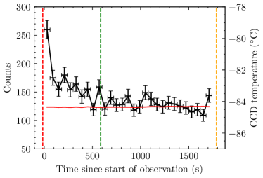
Figure 10: Example FWC light curve in eRASS1 at the $0.5<E<10$ keV band. The vertical red dashed line indicates when the filter wheel stopped rotating and stopped at the CLOSED position. The green dashed line indicates the reference cut-off time, which is 10 min after the red line. The orange line represents the time stamp when the filter wheel rotates again after the observation. Any events recorded between the red and green dashed lines are removed from the FWC dataset, and only events sandwiched between the green and orange dashed lines were considered. The width of the time bin is 60 s. The red horizontal line plots the CCD temperature in °C.

TM	Live time (s)
1	138257
2	117327
3	88255
4	125169
6	106495

Table 5: FWC live times of the TM1–4 and 6.

Figure 11 shows the FWC spectra combining all patterns overlaid with the best-fit models in red for TM1–4 and 6. All TMs possess an approximately flat spectrum between $\sim 1$–$9$ keV, then a variable cut-off between $9$–$10$ keV, depending on the TM. The variable cut-off is caused by the minimum ionisation particle threshold being defined on the raw event amplitudes instead of energy. Thus the cut-off varies according to the gain of each TM (Freyberg et al. 2020). Fluorescence lines including the most prominent $\@element{\mathrm{Al}}$ K$\alpha$ at $1.5$ keV and $\@element{\mathrm{Fe}}$ K$\alpha$ at $6.4$ keV are clearly visible. The flourescence lines are believed to originate within the cameras from the graded shield consisting primarily of $\@element{\mathrm{Al}}$, $\@element{\mathrm{Be}}$, plus some impurities including $\@element{\mathrm{Fe}}$ in the Be layer (Predehl et al. 2021). A gradual enhancement below $1$ keV is mainly induced by electronic noise.

The FWC spectral models provide a convenient way to subtract the instrumental background from the spectra of extended sources or diffuse emissions. These models aim to reproduce the FWC data as closely as possible instead of being fully physically motivated. The main components include power-law models to trace the overall shape of the continuum with an exponentially decaying tail $\sim 9$–$10$ keV to reproduce the cut-off. Fluorescence lines are reproduced by introducing gaussians at the appropriate energies. In addition to the florescence lines, gaussians are also introduced to modulate the model to accommodate small perturbations deviating from a perfectly smooth continuum.

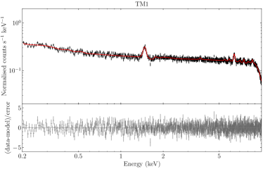
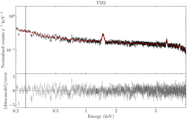
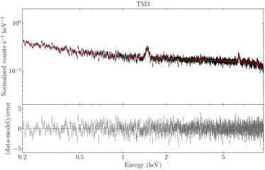
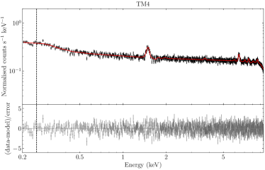
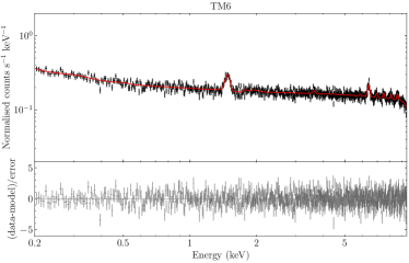
Figure 11: FWC spectra of all patterns for TM1–4 and 6. The best-fit FWC model is shown in red. The vertical dashed lines show the lowest energy the FWC model is employed due to variability considerations (Section B.1).

There is an assumption that the FWC spectra do not change with time and are stable despite variations in CCD temperature to justify our use of a single FWC model for each TM. In the Section B.1, we demonstrate the variabilities of the FWC spectra regarding the time evolution and the CCD temperature.

B.1 Variability of FWC spectra

Figure 12 shows the integrated FWC spectra for each eRASS, where eRASS0 corresponds to times in the commissioning, calibration and performance verification (CalPV) programme which preceded eRASS1. FWC observations were conducted for all TMs in eRASS0–2, while only TM4 and TM2 had FWC observations in eRASS3 and 5, respectively. For TM1, 3, 4 and 6, no noticeable variability was observed across $0.2<E<9$ keV. For TM2, the spectrum in eRASS5 is more enhanced $\lesssim 0.3$ keV, and slightly below the spectra of earlier eRASSs between $2$–$9$ keV. The lower particle background above $2$ keV is expected due to the well-known anti-correlation of Galactic cosmic ray flux with solar activity (the Sun was approaching maximum activity from eRASS0 to 5), where the solar wind provides some degrees of shielding to Galactic cosmic rays (Neher & Anderson 1962; Bulbul et al. 2020). Given that the FWC spectrum of TM2 is stable in the $0.25$–$2$ keV range, the energy range for spectral analysis of eRASS3–4 data is limited to $>0.25$ keV.

For all TMs at $E\lesssim 0.2$ keV, there is a clear trend of higher electronic noise for later eRASSs, despite the exact difference being dependent on the TM concerned. This could be the effect of CCD degradation caused by, for instance, radiation damage.

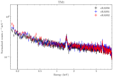
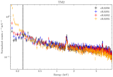
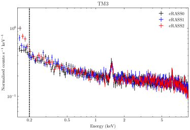
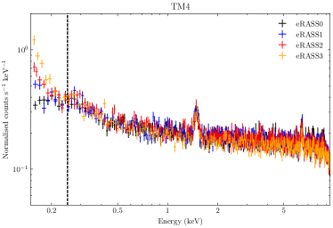
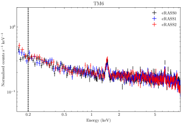
Figure 12: FWC Spectra of each eRASS including the CalPV phase. The vertical dashed lines indicate the energy below which variability sets in.

CCD temperature is expected to correlate with the electronic noise that contributing to the rising background at low energies. To investigate this effect, we extracted the CCD temperature records from the eROSITA housekeeping files to create GTIs which divide the FWC data into temperature bins of $1$ °C width. Figure 13 shows the FWC spectrum of each temperature bin. Similarly to time variability, no significant difference between spectra of each temperature is observed for TM1, 3 and 6 above $0.2$ keV. For TM2 and 4, for temperature bins centred at or above $-82$ °C, noticeable enhancements $\lesssim 0.25$ keV can be observed. While the shapes are similar, the cause of the enhancements is not necessarily identical. Further inspection reveals that all the events in the $-81$ °C bin of TM2 are from eRASS5, which means one is essentially looking at the same spectrum shown in Fig. 12. Therefore, it is unclear whether the enhancement is a pure result of the degradation of the CCD or it also involves genuine CCD temperature dependence. It is most likely that both effects are present. On the other hand, despite most of the events in the $-81$ and $-80$ °C bins being recorded in eRASS3 in TM4, the eRASS3 spectrum of TM4 (Fig. 12) includes events also from lower CCD temperatures. The eRASS3 spectrum between $0.15$ and $0.25$ keV is slightly lower compared to the $-80$ °C and $-81$ °C spectra suggests the events recorded at lower temperatures have suppressed the enhancement in the eRASS3 spectrum. Hence, at least for TM4, one could see that both CCD degradation and temperature affect the electronic noise component $\lesssim 0.25$ keV.

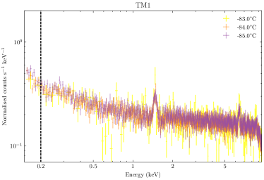
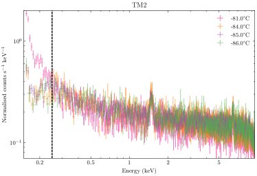
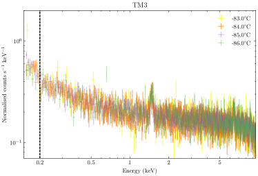
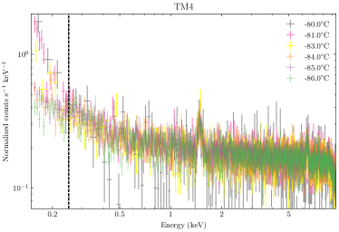
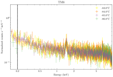
Figure 13: FWC Spectra of as a function of CCD temperature. Each temperature bin has a width of $1$ °C centering at the temperature indicated in the legend. The size of the error bars reflect the duration the detector was in the corresponding temperature when the FWC observations were taken. The vertical dashed lines indicate the energy below which variability sets in.

For each TM, we have identified the lowest energy that the FWC spectrum is stable, namely, $0.2$ keV for TM1, 3 and 6, and $0.25$ keV for TM2 and 4. These energies were plotted on Fig. 11, 12 and 13 as reference. Naturally, they serve as the lowest energies to which the corresponding FWC models should be applied. For our purpose, they also set the lowest energies for our spectral analysis.

Appendix C Position and pointing of SRG/eROSITA with respect to the magnetosphere

We also checked the position of SRG/eROSITA with respect to the Sun-Earth-L2 line at the times of our shadowing observation periods. Table 6 gives the distances in geocentric solar ecliptic (GSE) coordinates, in units of Earth radii ($R_{\mathrm{E}}$). In this right-handed system the $+X$ axis points towards the Sun, with the $+Z$ axis towards the North, $-Y$ in the ecliptic plane in the direction of planetary motion. $YZ=\sqrt{Y^{2}+Z^{2}}$ is the distance from the Sun-Earth-L2 line, the larger the value, the more likely SRG/eROSITA is outside of the magnetosheath. The radius of the bow shock at L2 is usually assumed to be of order $100\,R_{\rm E}$ (for a review on Earth’s magnetosphere, see, e.g. (Borovsky & Valdivia 2018) and references therein). During the four eRASSs the values of $YZ$ ranged between 44 and 139 $R_{\rm E}$, while our targets were observed mostly at $YZ>90\,R_{\rm E}$, which is outside the magnetosheath. Enhanced variable background was found more frequently for lower values.

eROSITA target ($\lambda,\beta$)	eRASS	Dates	X	Y	Z	YZ
	1	2020-02-27 – 2020-03-13	-234.07	111.07	1.00	111.42
Cha II & III $(246\degr,-61\degr)$	2	2020-08-26 – 2020-09-12	-239.43	102.64	7.98	103.68
	3	2021-02-11 – 2021-03-10	-238.59	84.28	25.69	91.48
	4	2021-08-20 – 2021-09-06	-238.50	90.68	27.46	95.84
	1	2020-04-10 – 2020-04-14	-185.07	91.22	-58.26	108.27
CrA $(284\degr,-14\degr)$	2	2020-10-13 – 2020-10-17	-183.05	75.48	-67.20	101.11
	3	2021-04-08 – 2021-04-14	-185.93	66.78	-70.49	97.20
	4	2021-10-12 – 2021-10-17	-186.52	47.65	-72.95	87.26
	1	2020-03-07 – 2020-03-15	-224.82	122.12	-11.05	122.70
Oph $(250\degr,-1\degr)$	2	2020-09-06 – 2020-09-15	-228.70	114.73	-7.48	115.12
	3	2021-02-23 – 2021-03-12	-230.16	101.03	7.81	102.24
	4	2021-08-31 – 2021-09-10	-228.11	102.67	7.63	103.33

Table 6: Average position of SRG/eROSITA in geocentric solar ecliptic (GSE) coordinates with respect to the Sun-Earth-L2 line at the times of the X-ray shadowing observations (with ecliptic look direction indicated), in units of Earth radii. For details on the orbit see (Freyberg et al. 2020).

At the times of Oph observations, SRG/eROSITA was close to the ecliptic plane (low $Z$ values) and looking almost in the ecliptic plane ($\beta\sim-1^{\circ}$). In March (eRASS1 and 3), eROSITA was thus looking through the magnetosphere, while in September (eRASS2 and 4), it was looking away when Ophiuchus was in the field of view. From observations of the South Ecliptic Pole, which was observed every four hours in Survey mode, we could not find any significant difference when being above or below the magnetosphere.

Appendix D Posterior distributions of model parameters

We present the projected posterior distributions of the model parameters of Cha II & III in Fig. 14. No significant correlations between LHB and SWCX parameters are found. The results for CrA and Oph are similar, thus, are not presented for the sake of brevity.

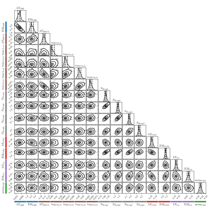
Figure 14: Two-dimensional projections of the posterior distributions of all the model parameters of Cha II & III. The contours represent $1$, $2$ and $3\,\sigma$ confidence levels. The parameters are colour-coded using the same colours as in the spectra shown in Fig. 5, 6 and 7. The units are the same as in Table 2.

Appendix E Comparison of LHB properties using AtomDB version 3.0.3

All the spectral fitting results reported in Sect. 4 are done using the latest AtomDB version 3.0.9. However, to ensure a direct comparison of LHB temperature and EM with the most recent and relevant measurement of the LHB by Liu et al. (2017), we repeat the spectral fitting using AtomDB version 3.0.3. While the AtomDB version adopted by Liu et al. (2017) is not specified in their work, version 3.0.3 appears to be a reasonable choice as it would be the latest version six months before its publication, taking into account the reviewing process.

We find marginally significant differences towards Cha II & III in the foreground components; otherwise, the background components are unaffected. Best-fit parameters of Oph and CrA are not affected by the change of AtomDB version (see Table 7). The increase of $kT_{\mathrm{LHB}}$ of Cha II & III from $0.084^{+0.004}_{-0.004}$ keV (v3.0.9) to $0.089^{+0.003}_{-0.005}$ keV (v3.0.3) would slightly impact the significance of the LHB temperature difference between the clouds we mentioned in Sect. 4. Using an older version of AtomDB appears to bring $kT_{\mathrm{LHB}}$ measured in Cha II & III closer to the other two clouds (Fig. 15) and the measurement of Liu et al. (2017) averaged across the whole sky. Nonetheless, the best-fit $kT_{\mathrm{LHB}}$ and $\mathrm{EM}_{\mathrm{LHB}}$ values of both versions are consistent with the measurement of Liu et al. (2017).

Table 7: Fit parameters of the spectral fitting using AtomDB version 3.0.3.

Cloud	Cha II & III	Oph	CrA
$kT_{\mathrm{LHB}}$	$0.089^{+0.003}_{-0.005}$	$0.100^{+0.007}_{-0.007}$	$0.109^{+0.010}_{-0.010}$
$\mathrm{EM}_{\mathrm{LHB}}$	$2.304^{+0.291}_{-0.216}$	$2.138^{+0.324}_{-0.279}$	$1.740^{+0.343}_{-0.266}$
$kT_{\mathrm{SWCX}}$	$0.108^{+0.003}_{-0.004}$	$0.109^{+0.002}_{-0.002}$	$0.105^{+0.004}_{-0.003}$
$n_{\mathrm{SWCX,e1}}$	$0.225^{+0.274}_{-0.187}$	$1.684^{+0.516}_{-0.566}$	$4.026^{+1.200}_{-1.157}$
$n_{\mathrm{SWCX,e2}}$	$0.446^{+0.325}_{-0.273}$	$4.927^{+0.642}_{-0.629}$	$4.306^{+1.239}_{-1.116}$
$n_{\mathrm{SWCX,e3}}$	$1.566^{+0.437}_{-0.348}$	$7.277^{+0.782}_{-0.750}$	$5.623^{+1.239}_{-1.253}$
$n_{\mathrm{SWCX,e4}}$	$2.671^{+0.602}_{-0.477}$	$8.857^{+0.807}_{-0.805}$	$5.681^{+1.277}_{-1.305}$
$N_{\mathrm{H,reg1}}$	$1.154^{+0.069}_{-0.056}$	$2.410^{+0.196}_{-0.191}$	$0.644^{+0.042}_{-0.038}$
$N_{\mathrm{H,reg2}}$	$1.486^{+0.070}_{-0.064}$	$3.442^{+0.210}_{-0.204}$	$1.930^{+0.059}_{-0.044}$
$N_{\mathrm{H,reg3}}$	$2.376^{+0.079}_{-0.069}$	$5.327^{+0.256}_{-0.215}$	$1.623^{+0.057}_{-0.050}$
$N_{\mathrm{H,reg4}}$	$4.348^{+0.122}_{-0.116}$	$6.377^{+0.417}_{-0.442}$	$3.670^{+0.086}_{-0.081}$
$kT_{\mathrm{CGM}}$	$0.183^{+0.002}_{-0.002}$	$0.272^{+0.010}_{-0.011}$	$0.205^{+0.004}_{-0.003}$
$\mathrm{EM}_{\mathrm{CGM}}$	$7.260^{+0.538}_{-0.487}$	$4.435^{+0.812}_{-0.656}$	$13.674^{+0.719}_{-0.732}$
$kT_{\mathrm{Cor}}$	$0.756^{+0.019}_{-0.020}$	$0.711^{+0.015}_{-0.014}$	$0.586^{+0.008}_{-0.008}$
$\mathrm{EM}_{\mathrm{Cor}}$	$0.661^{+0.045}_{-0.040}$	$2.371^{+0.177}_{-0.157}$	$3.383^{+0.131}_{-0.134}$
$\mathrm{norm}_{\mathrm{CXB}}$	$0.236^{+0.003}_{-0.003}$	$0.285^{+0.007}_{-0.006}$	$0.224^{+0.006}_{-0.006}$

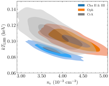
Figure 15: Posterior distributions of the temperature and electron density of the LHB using AtomDB version 3.0.3. The contours indicate the 1, 2 and 3 $\sigma$ confidence levels (enclose $\sim$ 39, 86 and 99% of the probability from the highest density).