How Sparse Can We Prune A Deep Network: A Geometric Viewpoint

Abstract

Overparameterization constitutes one of the most significant hallmarks of deep neural networks. Though it can offer the advantage of outstanding generalization performance, it meanwhile imposes substantial storage burden, thus necessitating the study of network pruning. A natural and fundamental question is: How sparse can we prune a deep network (with almost no hurt on the performance)? To address this problem, in this work we take a first principles approach, specifically, by merely enforcing the sparsity constraint on the original loss function, we’re able to characterize the sharp phase transition point of pruning ratio, which corresponds to the boundary between the feasible and the infeasible, from the perspective of high-dimensional geometry. It turns out that the phase transition point of pruning ratio equals the squared Gaussian width of some convex body resulting from the $l_{1}$-regularized loss function, normalized by the original dimension of parameters. As a byproduct, we provide a novel network pruning algorithm which is essentially a global one-shot pruning one. Furthermore, we provide efficient countermeasures to address the challenges in computing the involved Gaussian width, including the spectrum estimation of a large-scale Hessian matrix and dealing with the non-definite positiveness of a Hessian matrix. It is demonstrated that the predicted pruning ratio threshold coincides very well with the actual value obtained from the experiments and our proposed pruning algorithm can achieve competitive or even better performance than the existing pruning algorithms. All codes are available at: https://github.com/QiaozheZhang/Global-One-shot-Pruning

1 Introduction

Deep neural networks (DNNs) have continuously achieved stunning performance in the past decade. The success of DNN relies heavily on the overparametrization, which is manifested as several order of magnitudes more parameters than the number of datapoints. Despite the wide use of GPUs for acceleration, it still remains challenging in terms of the computation ability for deep networks. Moreover, for mobile devices and other small peripherals which have limited storage and computing capabilities, overparametrized networks will undoubted constitute huge burden. Therefore, it is of substantial importance to compress the deep networks while preserving its performance.

A key approach to compressing DNN models is network pruning, which was first introduced by Lecun in 1990[15]. Network pruning can substantially decrease the parameter count, reduce network complexity, and thus alleviate the computational burden of inference, resulting in decreased storage and computing requirements. The basic idea of network pruning is to devise metrics to evaluate the significance of parameters and then remove the insignificant ones. Model pruning can be roughly classified into structured and unstructured methods. Unstructured pruning are based on heuristic methods such as weight size[6], gradient[7], and Hessian statistics[15] etc, which sets unimportant parameters to zero to boost the sparsity while maintaining model performance. In contrast, structured pruning is a coarse-grained pruning method which normally use channels (or filters) as the basic pruning unit[17; 29; 24; 25; 18; 16; 9] and based on the metric of some channel importance.

Compared with the advances of network pruning algorithms, the theoretical results on network pruning are relatively less. Yang et al.[26] explored the impact of network pruning on model’s generalization ability, while He et al.[10] identified the relationship between the double descent phenomenon of network pruning and the learning distance. Despite of the above progresses, unfortunately, it still remains elusive about the fundamental limit of network pruning (while maintaining the performance). To tackle this problem, in this paper we’ll take a first principle approach (i.e. by merely imposing sparsity constraint on the loss function) and leverage powerful tools and theorems in high-dimensional geometry, such as Gaussian width and the Gordon’s Escape theorem, thus we are able to succinctly and very precisely characterize the phase transition point of network pruning. And along the exploration from geometric perspective, we also discover the mechanism why network pruning can drastically reduce the number of parameters without hurting the performance as well as the key factors that impact the effectiveness of network pruning.

1.1 Our contributions

Our main contributions can be summarized as follows:

1. Our work is the first to characterize the maximal pruning ratio of deep networks, whose result (Gauss width) turns out to be succinct and rather precise.

   Moreover, we demonstrate the significant influence of the loss function’s flatness and the magnitude of weight on the maximum pruning ratio of the network.

2. We present a novel one-shot pruning algorithm based on $l_{1}$-regularization, whose performance is competitive with or even better than the existing pruning algorithms. Additionally, we provide an improved spectrum estimation algorithm for large Hessian matrices so as to compute the Gaussian width.

3. We validate our pruning algorithm and theoretical predictions through experiments on CIFAR-10 and CIFAR-100 datasets[12] using multiple models. The experimental results demonstrate that our pruning algorithm is not only faster but also achieves better performance. Moreover, the maximum pruning degrees predicted by our theory align well with the actual values, with difference less than 1.2%.

1.2 Related Work

Pruning Methods:

Unstructured pruning involves removing unimportant weights without adhering to specific geometric shapes or constraints. Compared to structured pruning, it is easier to achieve higher sparsity while maintaining the same performance. Researchers have developed various methods to measure the importance of weights in the network. LeCun et al.[15] proposed the concept of optimal brain damage, which used second-derivative information to remove unimportant weights from the network. Han et al.[7] presented the train-prune-retrain method, which reduces the storage and computation of neural networks by learning only the significant connections. Yang et al.[27] employed the energy consumption of each layer to determine the pruning order and developed latency tables that employed greed to identify the layers that should be pruned. Guo et al.[5] proposed dynamic network surgery, which reduced network complexity significantly by pruning connections in real-time. In contrast to the previous method, Guo et al. included connected splicing throughout the process to avoid incorrect pruning. By adding a learning process to the process of filtering important and unimportant parameters, it was possible to identify the optimal parameters. Frankle et al.[1] proposed pruning by iteratively removing part of the small weights, and based on Frankle’s iterative pruning, Sreenivasan et al.[21] introduced $l_{2}$-norm to constrain the magnitude of unimportant parameters during iterative training. Our work adopts a one-step pruning approach, using $l_{1}$-norm, which is the convex approximation of the $l_{0}$-norm to constrain the magnitude of unimportant weights, and then pruning the weights below a certain threshold.

Theoretical Advances in Understanding Neural Networks:

Despite a promising performance in empirical data, providing theoretical guarantees for neural networks remains challenging. Ravid Schwartz-Ziv et al.[19] have explained the training dynamics of neural networks from the information theoretic perspective. The most prominent approach to understanding neural networks is the linearization or neural tangent kernel (NTK) technique[11]. This method assumes that the dynamics of gradient descent can be approximated by gradient descent on a linear regression instance with fixed feature representation. Using this linearization technique, it is possible to prove convergence to a zero training loss point. Additionally, Larsen et al.[14] studied the training dimension threshold of the network from a geometric point of view, which shows that the network can be trained successfully with less degrees of freedom (DoF) in affine subspace, but the burn-in affine subspace needs a good starting point and also the lottery subspace is greatly affected by the principal components of the entire training trajectory. Therefore, essentially the DoF result in [14] provides very limited knowledge about the maximum pruning ratio, which is exactly the main subject of our work. The other differences between our work and [14] include: 1) We present a rather precise value of Gaussian width of an ellipsoid, while [14] provides a range. 2) Our framework can handle arbitrary loss functions, rather than the specific quadratic loss functions in [14]. 3) We address the challenges encountered in computing the Gaussian width, which are untouched in [14].

2 Problem Setup

We start from defining the fundamental objective of network pruning , then by relaxing the $l_{0}$-norm to the $l_{1}$-norm, we obtain a convex body which corresponds to the sublevel set of the regularized loss function and thus we can thus leverage powerful tools in high-dimensional (convex) geometry.

Model Setup.

Let $\hat{y}=f({\bf{w}},{\bf{x}})$ be a deep neural network with weights ${\bf{w}}\in\mathbb{R}^{D}$ and inputs ${\bf{x}}\in\mathbb{R}^{K}$. For a given training data set $\{{\bf x}_{n},{\bf y}_{n}\}^{N}_{n=1}$ and loss function $\ell$, the empirical loss landscape is defined as $\mathcal{L}({\bf w})=\frac{1}{N}\sum^{N}_{n=1}\ell(f({\bf w},{\bf x}_{n}),{\bf y}_{n}).$ We employ classification as our primary task, where ${\bf y}\in\{0,1\}^{k}$ with $k$ is the number of classes, and $\ell(f({\bf w},{\bf x}_{n}),{\bf y}_{n})$ is the cross-entropy loss.

Loss Sublevel Sets.

A loss sublevel set of a network is the set of all weights ${\bf w}$ that achieve the loss up to $\epsilon$:

$$S(\epsilon):=\{{\bf w}\in\mathbb{R}^{D}:\mathcal{L}({\bf w})\leq\epsilon\}.$$ (1)

Pruning Objective.

In general, network pruning can be categorized as the following optimization problem:

$$\min\ \mathcal{L}({\bf w})+\lambda\lVert{\bf w}\rVert_{0}$$ (2)

where ${\bf w}$ is the weights of network model, $\lambda$ is the regularization penalty factor and $\lVert\cdot\rVert_{0}$ is the standard $l_{0}$-norm. However, since the $l_{0}$-norm is non-convex, the widely used gradient descent algorithm cannot optimize this function. Consider that $l_{1}$-norm can be regarded as the convex relaxation of $l_{0}$-norm, the sparse network can also be obtained by using $l_{1}$-norm. In this paper, the optimization objective of the network is adapted to:

$$\min\ \mathcal{L}({\bf w})+\lambda\lVert{\bf w}\rVert_{1}$$ (3)

After completing the network training, the network weights are pruned in ascending order of magnitude, and the performance of the sparse network is evaluated on the test set. The correlation between the sparsity level and the network’s test accuracy is illustrated in Figure 2, Figure 4 and Table 2.

Successful Pruning.

Define the loss of the dense network as $\epsilon$, use ${\bf w}_{p}$ to represent the weight of the sparse network, where $p$ is the degree of sparsity, and the definition of successful pruning of the network is:

$$S(\epsilon)\cap\{{\bf w}_{p}\}\neq\emptyset$$ (4)

3 Theory of Maximum Network Pruning Ratio

In this section, we address the issue of sublevel sets intersecting sparse weights by utilizing Gordon’s escape theorem from high-dimensional geometry. Initially, we present the concept of Gaussian width and Gordon’s escape theorem. Subsequently, we tightened the Gaussian width of the ellipsoid by concentration of measure and broaden its applicability to various forms of loss functions. Lastly, we conduct a comparative analysis between the ellipsoid Gaussian width proposed by [14] and ours.

3.1 Network Pruning: Phase Transition

Definition 1 (Gaussian Width)

. The gaussian width of s subset $S\in\mathbb{R}^{D}$ is given by:

$$w(S)=\frac{1}{2}\mathbb{E}\sup\limits_{{\bf x},{\bf y}\in S}\left<{\bf g,x-y}\right>,{\bf g}\sim\mathcal{N}({\bf 0},{\bf I}_{D\times D}).$$ (5)

Gordon’s escape theorem. The Gaussian width $w(S)$ of a set $S$, at least when that set is contained in a unit sphere around the origin, in turn characterizes the probability that a random subspace intersects that set, through Gordon’s escape theorem[4]:

Theorem 1 (Escape Theorem)

Let $S$ be a closed subset of the unit sphere in $\mathcal{R}^{D}$. If $k>w(S)^{2}$, then a $d=D-k$ dimensional subspace $Y$ drawn uniformly from the Grassmannian satisfies[4]:

$$\mathbb{P}(Y\cap S=\emptyset)\geq 1-3.5\exp[-(k/\sqrt{k+1}-w(S))^{2}/18].$$ (6)

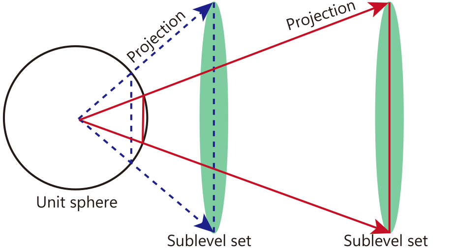
Figure 1: Effect of projection distance on projection size and intersection probability.

For using Gordon’s escape theorem in pruning works, we need to project the subset $S$ to the pruning point ${\bf w}_{p}$, where $p$ represents the pruning ratio. Therefore, we define the projection operation as follows:

$$\mathcal{P}({\bf w}_{p},S)=\{\frac{{\bf x-w}_{p}}{\|{\bf x-w}_{p}\|_{2}},{\bf x}\in S\}$$ (7)

Consider two manifolds with equal width, it can be observed that as the distance from the sphere increases, the projected size on the sphere decreases, leading to a reduced probability of intersection with the sphere. This relationship is visually depicted in Figure 1. Under the projection setting, the escape theorem of the pruning work is adjusted to:

Theorem 2 (Network Pruning Escape Theorm)

Let $S$ be a closed subset of the unit sphere in $\mathcal{R}^{D}$. If $k>w(\mathcal{P}({\bf w}_{p},S)^{2}$, then a $d=D-k$ dimensional subspace $Y$ drawn uniformly from the Grassmannian and centered at ${\bf w}_{p}$ satisfies:

$$\mathbb{P}(Y\cap S=\emptyset)\geq 1-3.5\exp[-(k/\sqrt{k+1}-w(\mathcal{P}({\bf w}_{p},S))^{2}/18].$$ (8)

This theorem tells us that when the dimension of the sub-network is lower than $D-w(\mathcal{P}({\bf w_{0}},S)^{2}$, the subspace will not intersect with $S$, which means the loss of the sub-network is higher than $\epsilon$. Therefore, the pruning ratio threshold of the network $M$ can be expressed as:

$$T(M,{\bf w}_{p})=\frac{D-(D-w(\mathcal{P}({\bf w}_{p},S)^{2})}{D}=\frac{w(\mathcal{P}({\bf w}_{p},S)^{2}}{D}.$$ (9)

The maximum pruning ratio $T(M,{\bf w}_{p})$ is a function of the pruning ratio $p$, when $T(M,{\bf w}_{p})$ is greater than $p$, the proportion of network weights that can be pruned is larger than the selected pruning ratio. In such cases, setting $p$ as the pruning ratio would not adversely impact the performance of the network. Conversely, when $T(M,{\bf w}_{p})$ is smaller than $p$, the prunable ratio is lower than the chosen pruning ratio, and using $p$ as the pruning ratio results in performance degradation of the sparse subnetwork. Therefore, it is crucial to determine a value of $p$ such that $T(M,{\bf w}_{p})$ equals $p$, which serves as the threshold for the network pruning ratio.

3.2 Gaussain Width of the Quadratic Well

We leverage tools including high-dimensional statistics, with a particular focus on the concentration of measure derived from measure theory. This enables us to present a rather precise expression for the Gaussian width of the ellipsoid in the context of high-dimensional scenarios.

Lemma 1

Give an ellipsoid $S(\epsilon)$ defined by a quadratic form: $S(\epsilon):=\{{\bf w}\in\mathbb{R}^{D}:\frac{1}{2}{\bf w}^{T}{\bf H}{\bf w}\leq\epsilon\}$ where ${\bf w}\in\mathbb{R}^{D}$ and ${\bf H}\in\mathbb{R}^{D\times D}$ is a symmetric, positive definite Hessian matrix. Loss sublevel set $S(\epsilon)$ defined by ${\bf H}$ is an ellipsoidal body with the Gaussian width:

$$w(S(\epsilon))\approx(2\epsilon\mathrm{Tr}({\bf H}^{-1}))^{1/2}=(\sum_{i}r_{i}^{2})^{1/2}$$ (10)

where $r_{i}=\sqrt{2\epsilon/\lambda_{i}}$ is the radius of ellipsoidal body and $\lambda_{i}$ is the $i$-th eigenvalue of ${\bf H}$.

The proof of Lemma 1 is in Appendix C.1.

3.3 Gaussian Width of the Projected Quadratic Well

In the paper by Larsen et al.[14], it is assumed that the loss function is a quadratic well, which limits the loss function used in network training. In order to push the theory of the maximum pruning ratio of the network to the general situation, we will not directly limit the network loss function to a quadratic form.

Consider a well-trained deep neural network model $M_{0}$ with weights ${\bf w}_{0}$, perform a Taylor expansion of $\mathcal{L}({\bf w})$ at ${\bf w}_{0}$:

$$\mathcal{L}({\bf w})=\mathcal{L}({\bf w}_{0})+({\bf w-w_{0}}){\bf G}+\frac{1}{2}({\bf w-w_{0}})^{T}{\bf H}({\bf w-w_{0}})+\Delta.$$ (11)

where ${\bf G}$ and ${\bf H}$ denote the first and second derivatives of $\mathcal{L}({\bf w})$ with respect to the model parameters ${\bf w}$, and $\Delta$ represents the higher order terms in the Taylor expansion which can be ignored.
For a well-trained deep neural network model, its first derivatives of $\mathcal{L}({\bf w})$ satisfy ${\bf G=0}$. Consequently, the loss sublevel set $S(\epsilon)$ can be expressed as:

$$S(\epsilon,{\bf w}_{0})=\{\hat{{\bf w}}\in\mathbb{R}^{D}:\frac{1}{2}\hat{{\bf w}}^{T}{\bf H}\hat{{\bf w}}\leq\hat{\epsilon}\}$$ (12)

where $\hat{\epsilon}=\epsilon-\mathcal{L}({\bf w}_{0})$ and $\hat{{\bf w}}={\bf w-w}_{0}$. Therefore, the Gaussian width of $S(\epsilon,{\bf w}_{0})$ becomes:

$$w(S(\epsilon,{\bf w}_{0}))=(2\hat{\epsilon}\mathrm{Tr}({\bf H}^{-1}))^{1/2}=(\sum_{i}\hat{r}_{i}^{2})^{1/2}\quad\text{with}\ \hat{r}_{i}=\sqrt{2\hat{\epsilon}/\lambda_{i}}$$ (13)

We next project the loss sublevel set $S(\epsilon,{\bf w}_{0})$ onto the surface of the unit sphere centered at ${\bf w}_{p}$:

Lemma 2

Consider a projection $\mathcal{P}({\bf w}_{p},S)$ defined in Eq.(7) and the projection distance $R=\|{\bf w}_{0}-{\bf w}_{p}\|_{2}$ from the pruning start point ${\bf w}_{0}$ to the chosen pruning point ${\bf w}_{p}$. Larsen et al.[14] outline the Gaussian width of the projected quadratic well is adjusted to:

$$w(\mathcal{P}({\bf w}_{p},S(\epsilon,{\bf w}_{0})))=(\sum_{i}\frac{\hat{r}_{i}^{2}}{R^{2}+\hat{r}_{i}^{2}})^{1/2}$$ (14)

It is important to note, however, this formula is an approximation and may lead to a theoretical prediction that is smaller than the actual predicted value. Nevertheless, empirical findings suggest that this formulation does not significantly underestimate theoretical predictions. Additionally, employing approximate calculations is simpler and entails considerably less computational burden compared to exact computations.

3.4 Comparison

The difference between our results and the Gaussian width demonstrated by Larsen et al. is shown in Table 1. One of the most notable distinctions between the Gaussian width we have proven and other measures is that our established Gaussian width is not represented as an interval but as a precise and definite value.

Table 1: Difference between Values.

	Value	Loss	Radius
Larsen et al.[14]	$[(\sqrt{\frac{2}{\pi}}\sum_{i}\frac{r_{i}^{2}}{R^{2}+r_{i}^{2}})^{1/2},(\sum_{i}\frac{r_{i}^{2}}{R^{2}+r_{i}^{2}})^{1/2}]$	Quadratic well	$\sqrt{2\epsilon/\lambda_{i}}$
Ours	$(\sum_{i}\frac{\hat{r}_{i}^{2}}{R^{2}+\hat{r}_{i}^{2}})^{1/2}$	Any form	$\sqrt{2(\epsilon-\mathcal{L}(\bf{w_{0}}))/\lambda_{i}})$

4 Approximate Calculation of Gaussian Width

In practical experiments, determining the Gaussian width of the ellipsoid defined by the network loss function is a challenging task. There are two primary challenges encountered in this section: 1. the computation of eigenvalues for high-dimensional matrices poses significant difficulty; 2. the network fails to converge perfectly to the extremum, leading to a non-positive definite Hessian matrix for the loss function. In this section, we tackle these challenges through the utilization of a fast eigenspectrum estimation algorithm and an algorithm that approximates the Gaussian width of a deformed ellipsoid body. These approaches effectively address the aforementioned problems.

4.1 Improved SLQ (Stochastic Lanczos Quadrature) Spectrum Estimation

Calculating the eigenvalues of large matrices has long been a challenging problem in numerical analysis. One widely used method for efficiently computing these eigenvalues is the Lanczos algorithm, which is presented in Appendix B. However, due to the huge amount of parameters of the deep neural network, it is still impractical to use this method to calculate the eigenspectrum of the Hessian matrix of a deep neural network. To tackle this problem, Yao et al.[28] proposed SLQ(Stochastic Lanczos Quadrature) Spectrum Estimation Algorithm, which estimates the overall eigenspectrum distribution based on a small number of eigenvalues obtained by Lanczos algorithm. This method enables the efficient computation of the full eigenvalues of large matrices. The specifics of this algorithm are provided in Appendix B.

In general, the Lanczos algorithm is not capable of accurately computing zero eigenvalues, and this limitation becomes more pronounced when the SLQ algorithm has a small number of iterations. Similarly, vanishingly small eigenvalues are also ignored by Lanczos. However, in a well-trained large-scale deep neural network, the experiment found that the network loss function hessian matrix has a large number of zero eigenvalues and vanishingly small eigenvalues. In the Gaussian width of the ellipsoid, the zero eigenvalues and vanishingly small eigenvalues have the same effect on the width (insensitive to other parameters), and we collectively refer to these eigenvalues as the "important" eigenvalues. We divide the weight into 100 parts from small to large, calculate the second-order derivative (including partial derivative) of smallest weight in each part, and sum the absolute values of all second-order derivatives of the weight, which corresponds to $l_{1}$-norm of a row in hessian matrix, and the row $l_{1}$-norm is zero or a vanishingly small corresponds to an "important" eigenvalue, the experimental results can be seen in the first column of Figure 3, from which the number of missing eigenvalues of the SLQ algorithm can be estimated, we then add the same number of 1e-30 as the missing eigenvalues in the Hessian matrix eigenspectrum.

4.2 Gaussian Width of the Deformed Ellipsoid

After effective training, it is generally assumed that a deep neural network will converge to the global minimum of its loss function. However, in practice, even after meticulous tuning, the network tends to oscillate around the minimum instead of converging to it. This leads to that the Hessian matrix of the loss function would be non-positive definite, and the resulting geometric body defined by this matrix would change from an expected ellipsoid to a hyperboloid, which is unfortunately nonconvex. To quantify the Gaussian width of the ellipsoid corresponding to the perfect minima, we propose to approximate it by convexifying the deformed ellipsoid through replacing the associated negative eigenvalues with its absolute value. This processing turns out to be very effective, as demonstrated by the experimental results.

Lemma 3

Consider a well-trained neural network $M$ with weights ${\bf w}$, whose loss function defined by ${\bf w}$ has a Hessian matrix ${\bf H}$. Due to the non-positive definiteness of ${\bf H}$, there exist negative eigenvalues. Let the eigenvalue decomposition of ${\bf H}$ be ${\bf H}={\bf v}^{T}{\bf\Sigma v}$, where ${\bf\Sigma}$ is a diagonal matrix of eigenvalues. Let ${\bf D}={\bf v}^{T}{\bf|\Sigma|v}$, where $|\cdot|$ means absolute operation. the geometric objects defined by H and D are $S(\epsilon):=\{{\bf w}\in\mathbb{R}^{D}:\frac{1}{2}{\bf w}^{T}{\bf H}{\bf w}\leq\epsilon\}$ and $\hat{S}(\epsilon):=\{{\bf w}\in\mathbb{R}^{D}:\frac{1}{2}{\bf w}^{T}{\bf D}{\bf w}\leq\epsilon\}$, then:

$$w(S(\epsilon))\approx w(\hat{S}(\epsilon))$$ (15)

The proof of Lemma 3 is in Appendix C.2.

Lemma 3 indicates that if the deep neural network converges to a vicinity of the global minimum of the loss function, the Gaussian width of the deformed ellipsoid body can be approximated by taking the convex hull of $S(\epsilon)$. Experimental results demonstrate that the two approximation methods, namely setting negative features to zero and taking absolute values, yield nearly indistinguishable outcomes.

5 Experiments

In this section, we experimentally validate our pruning method and upper bound on network pruning using the Escape Theorem.

Tasks.

We evaluate our pruning algorithm and maximum pruning ratio on (Task 1) CIFAR-10[12] on Full-Connect-5(FC-5) and Full-Connect-12(FC-12), (Task 2) CIFAR-10 on AlexNet[13] and VGG-16[20], CIFAR-100[12] on ResNet-18 and ResNet-50[8]. We make use of theoretical principles to anticipate the pruning ratio limit of the network, followed by an evaluation of the sparse sub-networks performance at different sparse ratios on both training and test data. Specifically, we calculate accuracy and loss metrics to quantify their performance. Finally, we compare the predicted upper bound on the pruning ratio with the actual maximum pruning ratio and evaluate whether they match.

Network Pruning.

To identify which weights to prune in the network, we incorporate $l_{1}$-regularization during network training and sort weights in ascending order according to their magnitude. We select weights to be pruned based on their magnitude, giving priority to smaller weights. Note that the pruning process excludes the weights of the bias and batch normalization layers. Taking ${\bf w}_{0}$ as the initial pruning point and calculating the corresponding value of $R$ for different pruning ratios. We then plot the corresponding curve of the theoretically predicted pruning ratio and the calculated $R$ in the same graph. The intersection point of these two curves is taken as the upper bound of the theoretically predicted pruning ratio.

Detailed descriptions of datasets, networks, hyper-parameters and eigenspectrum adjustment can be found in Section A of the Appendix.

5.1 Comparison of Pruning Effectiveness

We validated our proposed global one-shot pruning algorithm(GOP) on the task above. We compared our approach with pruning algorithms proposed by Sreenivasan et al.[21], including Rare Gems (RG), Rare Gems Reinit (RG-R), and Rare Gems Mask and Shuffle (RG-MS). Dense network accuracy is obtained by taking $l_{1}$-regularization parameter to zero with other hyper-parameters is the same as pruning algorithm. Table 2 shows the pruning performance of the above algorithms, our pruning algorithm is the fastest and best performing than other algorithms.

Table 2: Performance comparison of various pruning algorithms.

Dataset	Model	Dense Acc	Sparsity	Test Acc@top-1 | Run Epochs
				GOP	RG	RG-R	RG-MS
CIFAR10	FC-5	59.07%	1.7%	60.34% | 200	58.6% | 400	58.71% | 400	54.8% | 400
	FC-12	53.37%	1.0%	60.59% | 200	54.18% | 400	10.00% | 400	10.40% | 400
	AlexNet	88.82%	1.5%	89.69% | 200	86.11% | 400	85.24% | 400	11.19% | 400
	VGG-16	90.86%	0.2%	88.57% | 200	58.88% | 400	41.68% | 400	10.00% | 400
CIFAR100	ResNet-18	69.29%	2.2%	69.84% | 200	69.32% | 400	64.18% | 400	63.65% | 400
	ResNet-50	73.10%	2.6%	74.11% | 200	72.22% | 400	64.95% | 400	64.63% | 400

5.2 Pruning Upper Bound Theory Validation

We validated our prediction results on Task1 and Task2 for the upper bound of network pruning.

Task 1.

Figure. 2 shows the sparsity-accuracy trade-off in Full-Connect-5(FC-5) and Full-Connect-12(FC-12) trained on CIFAR-10 with $l_{1}$-regularization. Since the two models are relatively small, the estimation algorithm can accurately predict the maximum network pruning ratio without adjustment. Figure. 2 provide compelling evidence of the high redundancy of deep neural networks. The theoretical upper bound we derive matches well with the practical maximum pruning ratio.

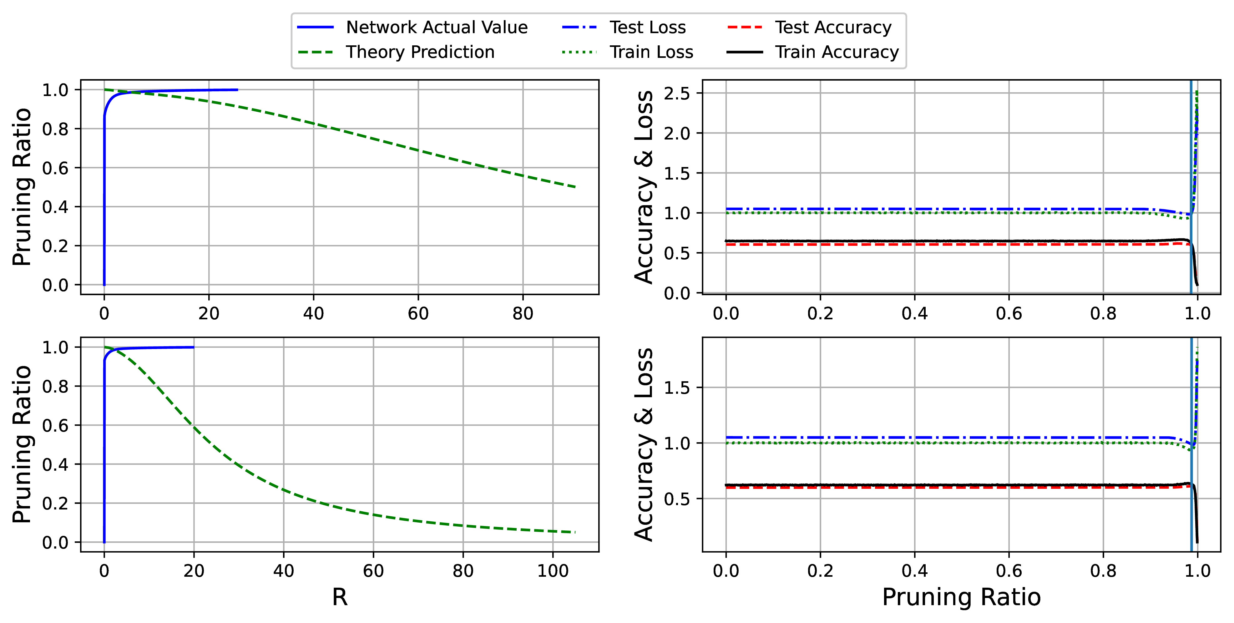
Figure 2: Comparison of the theoretical maximum pruning ratio with the value actually achieved. The two rows in the figure correspond to network models FC-5 and FC-12. The first row describes the pruning ratio as a function of R and its relationship to the pruning ratio of the network. The intersection of the two curves corresponds to the predicted maximum pruning ratio. The second row shows the accuracy and loss of the network with different pruning ratios on the training and test sets. For ease of visualization, the loss values are normalized, and the vertical line represents the theoretically predicted pruning rate.

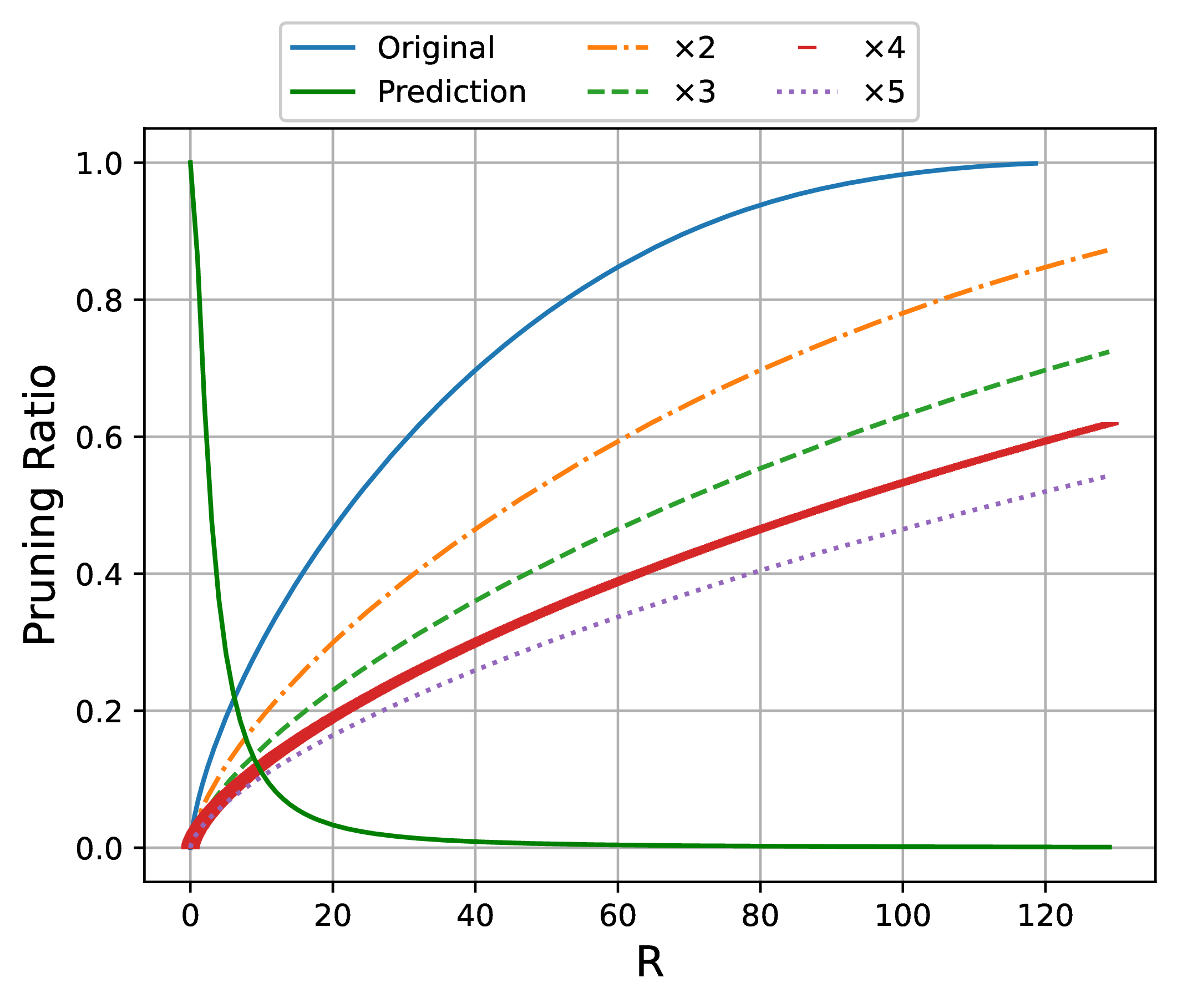
Figure 3: Pruning ratio prediction on different weight magnitude.

Task 2.

In large-scale network models such as AlexNet, VGG-16 on CIFAR-10 and ResNet-18, ResNet-50 on CIFAR-100, many parameters have second-order derivatives as zero or vanishingly small value, resulting in a corresponding number of "important" eigenvalues in the network Hessian matrix. Using the eigenvalue calculation adjustment scheme described earlier, we obtain the first and second column in Figure. 4, and the third column shows that our theoretical predictions are consistent with the actual values.

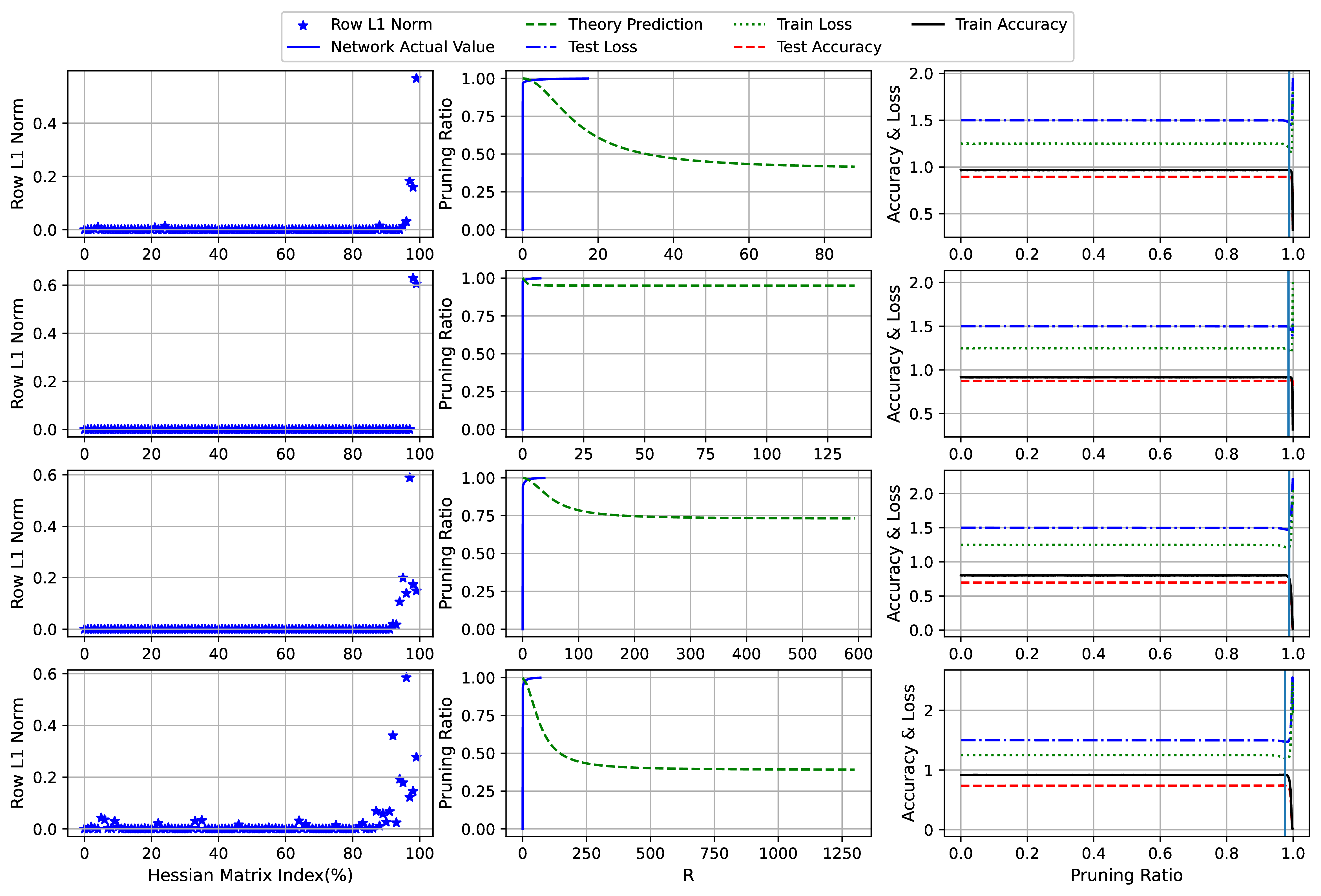
Figure 4: Comparison between the theoretical maximum pruning ratio and the actual value achieved. The four rows in the figure correspond to network models AlexNet, VGG-16, ResNet-18 and ResNet-50, respectively. The first column displays the row L1 norm curve of the Hessian matrix. With the SLQ algorithm supplemented based on the number of "important" eigenvalues displayed in the first column, the second and third columns are subsequently obtained. The second and third columns correspond to the first and second columns of Figure. 2.

5.3 Prediction Comparison

The numerical comparison between the predicted maximum pruning ratio and the actual value is shown in Table 3. The results in Table 3 exhibit a high degree of agreement between the predicted and actual values which demonstrate that our theoretical predictions effectively estimate the maximum network pruning ratio.

Table 3: Comparison of Predicted and Actual Values of maximum Pruning Ratio.

Dataset	Model	Prediction	Experimental Results	$\Delta$
CIFAR10	FC-5	98.6%	98.3%	0.3%
	FC-12	98.7%	99.0%	-0.3%
	AlexNet	98.8%	98.9%	-0.1%
	VGG-16	98.6%	99.8%	-1.2%
CIFAR100	ResNet-18	98.8%	97.9%	0.9%
	ResNet-50	97.6%	97.7%	-0.1%

5.4 Small Weights Benefits Pruning

We verify that high flatness is not equal to high pruning rate through hypothetical experiments. Considering that the hessian matrix of network $A$ and network $B_{1},B_{2},B_{3},B_{4}$ share eigenvalues $\{\lambda_{1},\lambda_{2},\lambda_{,}\dots,\lambda_{n}\}$, the weight magnitude of network $B_{1},B_{2},B_{3},B_{4}$ is 2,3,4,5 times that of network $A$, we take the eigenvalues and weights from a FC network trained without regularization. In this way, the gap between the curves will be more obvious. For other networks, the trend of the curve gap is consistent, the prediction of the maximum network pruning rate is shown in the Figure. 3. It is observed from Figure. 3 that as the magnitude of network weights increases, the capacity of the network to tolerate pruning decreases. The max pruning rate is affected not only by loss flatness but also the magnitude of weights. This finding, on the other hand, provides further evidence of the effectiveness of the $l_{1}$-norm in pruning tasks.

6 Conclusion

We explore the maximum pruning ratio of deep networks from the perspective of high dimensional geometry, which is enabled by defining the fundamental pruning objective as minimization of an $l_{1}$-regularized loss. By leveraging the powerful Gordon’s Escape theorem, we can for the first time characterize the sharp phase point of network pruning (namely, the maximum pruning ratio) in a very succinct form. As a byproduct, we provide a novel network pruning algorithm which is characteristic of a global one-shot pruning. Moreover, to address the challenges in computing the associated Gaussian width, we present an improved spectrum estimation for large Hessian matrices. Experiments demonstrate both the accuracy of our theoretical result and the high performance of our proposed pruning algorithm. Last, we also discover that networks with smoother loss landscapes and smaller weights have stronger pruning capability. This finding might offer insight for understanding and comparing various network pruning techniques.

Appendix A Experimental Details

In this section, we describe the datasets, models, hyper-parameter choices and eigenspectrum adjustment used in our experiments. All of our experiments are run using PyTorch 1.12.1 on Nvidia RTX3090s with ubuntu20.04-cuda11.3.1-cudnn8 docker.

A.1 Dataset

CIFAR-10.

CIFAR-10 consists of 60,000 color images, with each image belonging to one of ten different classes with size $32\times 32$. The classes include common objects such as airplanes, automobiles, birds, cats, deer, dogs, frogs, horses, ships, and trucks. The CIFAR-10 dataset is divided into two subsets: a training set and a test set. The training set contains 50,000 images, while the test set contains 10,000 images. [12]. For data processing, we follow the standard augmentation: normalize channel-wise, randomly horizontally flip, and random cropping.

CIFAR-100.

The CIFAR-100 dataset consists of 60,000 color images, with each image belonging to one of 100 different fine-grained classes[12]. These classes are organized into 20 superclasses, each containing 5 fine-grained classes. Similar to CIFAR-10, the CIFAR-100 dataset is split into a training set and a test set. The training set contains 50,000 images, and the test set contains 10,000 images. Each image is of size 32x32 pixels and is labeled with its corresponding fine-grained class. Augmentation includes normalize channel-wise, randomly horizontally flip, and random cropping.

A.2 Model

In all experiments, pruning skips bias and batchnorm, which have little effect on the sparsity of the network. Use non-affine batchnorm in the network, and the initialization of the network is kaiming normal initialization.

Full Connect Network(FC-5, FC-12).

We train a five-layer fully connected network (FC-5) and a twelve-layer fully connected network FC-12 on CIFAR-10, the network architecture details can be found in Table 4.

Table 4: FC-5 and FC-12 architecture used in our experiments.

Model	Layer Width
FC-5	1000, 600, 300, 100, 10
FC-12	1000, 900, 800, 750, 700, 650, 600, 500, 400, 200, 100, 10

AlexNet[13].

We use the standard AlexNet architecture. In order to use CIFAR-10 to train AlexNet, we upsample each picture of CIFAR-10 to $3\times 224\times 224$. The detailed network architecture parameters are shown in Table 5.

Table 5: AlexNet architecture used in our experiments.

Layer	Shape	Stride	Padding
conv1	$3\times 96\times 11\times 11$	4	1
max pooling	kernel size:3	2	N/A
conv2	$96\times 256\times 5\times 5$	1	2
max pooling	kernel size:3	2	N/A
conv3	$256\times 384\times 3\times 3$	1	1
conv4	$384\times 384\times 3\times 3$	1	1
conv4	$384\times 256\times 3\times 3$	1	1
max pooling	kernel size:3	2	N/A
linear1	$6400\times 4096$	N/A	N/A
linear1	$4096\times 4096$	N/A	N/A
linear1	$4096\times 10$	N/A	N/A

VGG-16[20].

In the original VGG-16 network, there are 13 convolution layers and 3 FC layers (including the last linear classification layer). We follow the VGG-16 architectures used in [2, 3] to remove the first two FC layers while keeping the last linear classification layer. This finally leads to a 14-layer architecture, but we still call it VGG-16 as it is modified from the original VGG-16 architectural design. Detailed architecture is shown in Table 6. VGG-16 is trained on CIFAR-10.

Table 6: VGG-16 architecture used in our experiments.

Layer	Shape	Stride	Padding
conv1	$3\times 64\times 3\times 3$	1	1
conv2	$64\times 64\times 3\times 3$	1	1
max pooling	kernel size:2	2	N/A
conv3	$64\times 128\times 3\times 3$	1	1
conv4	$128\times 128\times 3\times 3$	1	1
max pooling	kernel size:2	2	N/A
conv5	$128\times 256\times 3\times 3$	1	1
conv6	$256\times 256\times 3\times 3$	1	1
conv7	$256\times 256\times 3\times 3$	1	1
max pooling	kernel size:2	2	N/A
conv8	$256\times 512\times 3\times 3$	1	1
conv9	$512\times 512\times 3\times 3$	1	1
conv10	$512\times 512\times 3\times 3$	1	1
max pooling	kernel size:2	2	N/A
conv11	$512\times 512\times 3\times 3$	1	1
conv12	$512\times 512\times 3\times 3$	1	1
conv13	$512\times 512\times 3\times 3$	1	1
max pooling	kernel size:2	2	N/A
avg pooling	kernel size:1	1	N/A
linear1	$512\times 10$	N/A	N/A

ResNet-18 and ResNet-50[8].

We use the standard ResNet architecture and tune it for the CIFAR-100 dataset. The detailed network architecture parameters are shown in Table 7. ResNet-18 and ResNet-50 is trained on CIFAR-100.

Table 7: ResNet architecture used in our experiments.

Layer	ResNet-18	ResNet-50
conv1	$64,3\times 3\text{; stride:1; padding:1}$	$64,3\times 3\text{; stride:1; padding:1}$
block1	$\begin{pmatrix}64,3\times 3\text{; stride:1; padding:1}\\ 64,3\times 3\text{; stride:1; padding:1 }\end{pmatrix}\times 2$	$\begin{pmatrix}64,1\times 1\text{; stride:1; padding:0}\\ 64,3\times 3\text{; stride:1; padding:1}\\ 256,1\times 1\text{; stride:1; padding:0}\end{pmatrix}\times 3$
block1	$\begin{pmatrix}128,3\times 3\text{; stride:2; padding:1}\\ 128,3\times 3\text{; stride:1; padding:1 }\end{pmatrix}\times 2$	$\begin{pmatrix}128,1\times 1\text{; stride:1; padding:0}\\ 128,3\times 3\text{; stride:2; padding:1}\\ 512,3\times 3\text{; stride:1; padding:0}\end{pmatrix}\times 4$
block1	$\begin{pmatrix}128,s3\times 3\text{; stride:2; padding:1}\\ 256,3\times 3\text{; stride:1; padding:1}\end{pmatrix}\times 2$	$\begin{pmatrix}256,1\times 1\text{; stride:1; padding:0}\\ 256,3\times 3\text{; stride:2; padding:1}\\ 1024,1\times 1\text{; stride:1; padding:0}\end{pmatrix}\times 6$
block1	$\begin{pmatrix}512,3\times 3\text{; stride:2; padding:1}\\ 512,3\times 3\text{; stride:1; padding:0 }\end{pmatrix}\times 2$	$\begin{pmatrix}512,1\times 1\text{; stride:1; padding:1}\\ 512,3\times 3\text{; stride:2; padding:1}\\ 2048,1\times 1\text{; stride:1; padding:0}\end{pmatrix}\times 3$
avg pooling	kernel size:1; stride:1	kernel size:1; stride:1
linear1	$512\times 100$	$2048\times 100$

A.3 Train Hyper-parameter Setup

In this section, we will describe in detail the training hyper-parameters of the Global One-shot Pruning algorithm on multiple datasets and models. The various hyper-parameters are detailed in Table 8.

Table 8: Hyper Parameters used for different Datasets and Models.

Model	Dataset	Batch Size	Epochs	Optimizer	LR	Momentum	Warm Up	Weight Decay	CosineLR	Lambda
FC-5	CIFAR-10	128	200	SGD	0.01	0.9	0	0	N/A	0.00005
FC-12	CIFAR-10	128	200	SGD	0.01	0.9	0	0	N/A	0.00005
VGG-16	CIFAR-10	128	200	SGD	0.01	0.9	5	0	N/A	0.0001
AlexNet	CIFAR-10	128	200	SGD	0.01	0.9	5	0	True	0.00003
ResNet-18	CIFAR-100	128	200	SGD	0.1	0.9	5	0	True	0.00005
ResNet-50	CIFAR-100	128	200	SGD	0.1	0.9	5	0	True	0.00002

A.4 Sublevel Set Parameter Setup.

Given that the test data is often unavailable and the network can ensure the Hessian matrix is positive definite as much as possible by utilizing the training data for computation. Additionally, we generally assume that the training and test data share the same distribution, thus we use the training data to define the loss sublevel set as $\hat{\epsilon}=\epsilon-\mathcal{L}({\bf w}_{0})$. We compute the standard deviation of the network’s loss across multiple batches on the training data set and denote it by $\hat{\epsilon}$.

Table 9: Hyper Parameters used in SLQ Algorithm.

Model	Dataset	Runs	Iterations	Bins	Squared Sigma
FC-5	CIFAR-10	1	128	10000	1e-05
FC-12	CIFAR-10	1	128	10000	1e-05
VGG-16	CIFAR-10	1	128	100000	1e-10
AlexNet	CIFAR-10	1	96	100000	1e-10
ResNet-18	CIFAR-100	1	128	100000	1e-10
ResNet-50	CIFAR-100	1	128	100000	1e-10

A.5 Eigenspectrum Adjustment

The minimum eigenvalue from the eigenvalues obtained by the Lanczos algorithm still remains much larger than the minimum eigenvalue of the Hessian matrix. The default parameters used in the SLQ algorithm result in an eigenspectrum with a minimum eigenvalue greater than the eigenvalues obtained by the Lanczos algorithm, leading to an underestimation of the pruning ratio threshold and a significant deviation from the pruning phase transition point. To address this issue, we adjusted the SLQ algorithm parameters to match the minimum eigenvalue obtained by the Lanczos algorithm. SLQ algorithm parameters adjustment is discribed in Table 9. Considering that the Lanczos algorithm cannot calculate the zero eigenvalues and vanishingly small eigenvalues which is refered as "important" eigenvalues, the directly output spectrum will not contain the "important" eigenvalues, which is needed to be filled in the spectrum. We sorted the network weights in ascending order and divided them into 100 equal parts. For each weight, we compute the second derivative and calculate the sum of absolute values of the derivative (which corresponds to the $l_{1}$-norm of the row or column in the Hessian matrix). This allowed us to obtain the "important" eigenvalues in the Hessian matrix, which is added to the eigenspectrum obtained by the SLQ algorithm.

Appendix B Details of Algorithm

In this section, we present a detailed description of the classic Lanczos algorithm, a widely used numerical method in linear algebra. The algorithm follows a specific flow that culminates in the computation of an $m\times m$ triangular matrix, denoted as $\bf T$. By decomposing the eigenvalues of $\bf T$, we can obtain $m$ distinct eigenvalues of the Hermitian matrix $\bf A$. Algorithm 1 outlines the step-by-step procedure for the classic Lanczos algorithm, providing a comprehensive guide for its implementation. The algorithm requires the selection of the number of iterations, denoted as $m$, which determines the size of the resulting triangular matrix $\bf T$.

Input: a Hermitian matrix ${\bf A}$ of size $n\times n$, a number of iterations $m$

Output: a tridiagonal real symmetric matrix ${\bf T}$ of size $m\times m$

  initialization:

  1. Draw a random vector ${\bf v_{1}}$ of size $n\times 1$ from $\mathcal{N}$(0,1) and normalize it;

  2. ${\bf w^{{}^{\prime}}_{1}}={\bf A}{\bf v_{1}}$; $\alpha_{1}=<{\bf w^{{}^{\prime}}_{1}},{\bf v_{1}}>$; ${\bf w_{1}=w^{{}^{\prime}}_{1}}-\alpha_{1}{\bf v_{1}}$;

  3.

  for $j=2,...,m$ do

     1). $\beta_{j}=\lVert{\bf w_{j-1}}\rVert$;

     2).

• if $\beta_{j}=0$ then

• stop

• else

• ${\bf v_{j}=w_{j-1}}/\beta_{j}$

• end if

     3). ${\bf w_{j}^{{}^{\prime}}}={\bf A}{\bf v_{j}}$;

     4). $\alpha_{j}={\bf<w^{{}^{\prime}}_{j},v_{j}>}$;

     5). ${\bf w_{j}}={\bf w_{j}^{{}^{\prime}}}-\alpha_{j}{\bf v_{j}}-\beta_{j}{\bf v_{j-1}}$;

  end for

  4. ${\bf T}(i,i)=\alpha_{i},\ i=1,\dots,m$;

    ${\bf T}(i,i+1)={\bf T}(i+1,i)=\beta_{i},\ i=1,\dots,m-1$.

  return ${\bf T}$

Algorithm 1 The Lanczos Algorithm

Based on the Lanczos algorithm, Yao et al.[28] proposed a large-scale matrix eigenspectrum estimation algorithm. For details of the algorithm, see Algorithm 2

Input: A hermitian matrix ${\bf A}$ of size $n\times n$, Lanczos iterations $m$, ESD computation iterations $l$, gaussian kernel $f$ and variance $\sigma^{2}$.

Output: The spectral distribution of matrix ${\bf A}$

  for $i=2,...,l$ do

     1). Get the tridiagonal matrix ${\bf T}$ if size $m\times m$ through Lanczos algorithm;

     2). Compute $\tau_{k}^{(i)}$ and $\lambda_{k}^{(i)}$ from ${\bf T}$;

     3). $\phi_{\sigma}^{i}(t)=\sum^{m}_{k=1}\tau_{k}^{(i)}f(\lambda_{k}^{(i)};t,\sigma)$;

  end for

  4). $\phi(t)=\frac{1}{l}\sum^{l}_{i=1}\phi_{\sigma}^{i}(t)$

  return $\phi(t)$

Algorithm 2 SLQ(Stochastic Lanczos Quadrature) Spectrum Estimation Algorithm

Appendix C Theoretical Part Supplement

In this section, we provide details regarding the threshold of network pruning ratio, specifically, the dimension of the sublevel sets of quadratic wells.

C.1 Gaussian Width of the Quadratic Well

Gaussian width is an extremely useful tool to measure the complexity of a convex body. In our proof, we will use the following expression for its definition:

$$w(S)=\frac{1}{2}\mathbb{E}\sup\limits_{{\bf x},{\bf y}\in S}\left<{\bf g,x-y}\right>,{\bf g}\sim\mathcal{N}({\bf 0},{\bf I}_{D\times D})$$

Concentration of measure is a universal phenomenon in high-dimensional probability. Basically, it says that a random variable which depends in a smooth way on many independent random variables (but not too much on any of them) is essentially constant.[22]

Theorem C. 1

(Gaussian concentration) Consider a random vector ${\bf x}\sim\mathcal{N}({\bf 0},{\bf I}_{n})$ and an L-Lipschitz function $f$ : $\mathbb{R}^{n}\rightarrow\mathbb{R}$ (with respect to the Euclidean metric). Then for $t\geq 0$

$$\mathbb{P}(|f({\bf x})-\mathbb{E}f({\bf x})|\geq t)\leq\epsilon,\quad\epsilon=e^{-\frac{t^{2}}{2L^{2}}}.$$

Therefore, if $\epsilon$ is small, $f({\bf x})$ can be approximated as $f({\bf x})\approx\mathbb{E}f({\bf x})+\sqrt{-2L^{2}\mathrm{ln}\epsilon}$.

Lemma C. 1

Given a random vector ${\bf x}\sim\mathcal{N}({\bf 0},{\bf I}_{n})$ and the inverse of a positive definite Hessian matrix ${\bf Q=H^{-1}}$, where ${\bf H}\in\mathbb{R}^{n\times n}$, we have:

$$\mathbb{E}\sqrt{{\bf x^{T}Qx}}\approx\sqrt{\mathbb{E}{\bf x^{T}Qx}}$$

$Proof.$
1.) Concentration of ${\bf x^{T}Qx}$

Define $f({\bf x})={\bf x^{T}Qx}$, we have

$$f({\bf x}) ={\bf x^{T}Qx}$$

$$={\bf x^{T}U\Sigma U^{T}x} \quad\quad\text{Eigenvalue Decomposition of }{\bf Q}:\ {\bf Q=U\Sigma U^{T}}.$$

$$=\sum_{i=1}^{n}\lambda_{i}x_{i}^{2}$$ Invariance of Gaussian under rotation.

where $\lambda_{i}$ is the eigenvalue of ${\bf Q}$. The lipschitz constant $L_{f}$ of function $f({\bf x})$ is :

$$L_{f}=\max(|\frac{\partial f}{\partial{\bf x}}|)=\max(|2\lambda_{i}x_{i}|)$$

Let $g(x_{i})=2\lambda_{i}x_{i}$, whose lipschitz constant is $L_{g}=|2\lambda_{i}|$. Invoking Theorem 1, we have:

$$g(x_{i}) \approx\mathbb{E}g(x_{i})+\sqrt{-2(2\lambda_{i})^{2}\mathrm{ln}\epsilon_{1}}$$

$$=\sqrt{-8\lambda_{i}^{2}\mathrm{ln}\epsilon_{1}}.$$

Therefore, the lipschitz constant of $f({\bf x})$ can be approximated by:

$$L_{f} =max(\sqrt{-8\lambda_{i}^{2}\mathrm{ln}\epsilon_{1}}) =\sqrt{-8\mathrm{ln}\epsilon_{1}}\lambda_{max}$$

Invoking Theorem 1 again, we establish the concentration of $f({\bf x})$ as follows:

$$f({\bf x}) \approx\mathbb{E}f({\bf x})+\sqrt{-2(L_{f})^{2}\mathrm{ln}\epsilon_{2}}\quad\quad\quad\quad\quad\quad\quad\quad\quad\quad\quad\quad\quad \text{Theorem}\ \ref{theoremcgc}.$$

$$=\mathbb{E}f({\bf x})+4\sqrt{\mathrm{ln}\epsilon_{1}\mathrm{ln}\epsilon_{2}}\lambda_{max}$$

2.) Jensen ratio of $\sqrt{{\bf x^{T}Qx}}$:

$$\mathbb{E}\sqrt{f({\bf x})} \approx\mathbb{E}\sqrt{\mathbb{E}f({\bf x})+4\sqrt{\mathrm{ln}\epsilon_{1}\mathrm{ln}\epsilon_{2}}\lambda_{max}} \text{Concentration of }f({\bf x}).$$

$$\approx\sqrt{\mathbb{E}f({\bf x})}+\frac{2\sqrt{\mathrm{ln}\epsilon_{1}\mathrm{ln}\epsilon_{2}}\lambda_{max}}{\sqrt{\mathbb{E}f({\bf x})}} \text{ Taylor Expansion}.$$

Therefore, the Jensen ratio of $\sqrt{f({\bf x}}$) equals:

$$\frac{\mathbb{E}\sqrt{f({\bf x})}}{\sqrt{\mathbb{E}f({\bf x})}} =1+2\sqrt{\mathrm{ln}\epsilon_{1}\mathrm{ln}\epsilon_{2}}\frac{\lambda_{max}}{\sum_{i=1}^{n}\lambda_{i}}$$

$$=1+\delta$$

If ${\bf Q}$ is a Wishart matrix, i.e., ${\bf Q}={{\bf A}^{T}{\bf A}}$, where ${\bf A}$ is a random matrix whose elements are independently and identically distributed with unit variance, according to the Marchenko-Pastur law[23], the maximum eigenvalue of ${\bf Q}$ is approximately $4n$ and the trace of ${\bf Q}$ is approximately $n^{2}$. Therefore, the above Jensen ratio approaches to 1 with decaying rate $\mathcal{O}(\frac{1}{n})$.

For the inverse of a positive definite Hessian matrix which is of our concern, we take $\epsilon_{1}=\epsilon_{2}=10^{-4}$, numerical simulations show that when the dimension $n=10^{5}$, the corresponding $\delta$ in the above Jensen ratio is on the order of $10^{-3}$, which is in good agreement with the theoretical value and is arguably negligible. Similar as the case of above-discussed Wishart matrix, when the dimension $n$ increases, the value of $\delta$ will further decrease.

Definition C. 1

(Definition of ball) A (closed) $ball\ B(c,r)$ (in $\mathbb{R}^{D}$) centered at $c\in\mathbb{R}^{D}$ with radius $r$ is the set

$$B(c,r):=\{{\bf x}\in\mathbb{R}^{D}:{\bf x}^{T}{\bf x}\leq r^{2}\}$$

The set $B(0,1)$ is called the $unit\ ball$. An ellipsoid is just an affine transformation of a ball.

Lemma C. 2

(Definition of ellipsoid). An $ellipsoid\ S$ centered at the origin is the image $L(B(0,1))$ of the unit ball under an $invertible$ linear transformation $L:\mathbb{R}^{D}\rightarrow\mathbb{R}^{D}$. An ellipsoid centered at a general point $c\in\mathbb{R}^{D}$ is just the translate $c+S$ of some ellipsoid $S$ centered at the origin.

$Proof.$

$$L(B(0,1)) =\{{\bf Lx}:{\bf x}\in B(0,1)\}$$

$$=\{{\bf y}:{\bf L}^{-1}{\bf y}\in B(0,1)\}$$

$$=\{{\bf y}:({\bf L}^{-1}{\bf y})^{T}{\bf L}^{-1}{\bf y}\leq 1\}$$

$$=\{{\bf y}:{\bf y}^{T}({\bf LL}^{T})^{-1}{\bf y}\leq 1\}$$

$$=\{{\bf y}:{\bf y}^{T}{\bf Q}^{-1}{\bf y}\leq 1\}$$

where ${\bf Q}={\bf LL}^{T}$ is positive definite.
The radius $r_{i}$ along principal axis ${\bf e}_{i}$ obeys $r_{i}^{2}=\frac{1}{\lambda_{i}}$, where $\lambda_{i}$ is the eigenvalue of ${\bf Q}^{-1}$ and ${\bf e}_{i}$ is eigen vector.

Lemma C. 3

(Gaussian width of ellipsoid). Let $S$ be an ellipsoid in $\mathbb{R}^{D}$ defined by the positive definite matrix ${\bf H}\in\mathbb{R}^{D\times D}$:

$$S(\epsilon):=\{{\bf w}\in\mathbb{R}^{D}:\frac{1}{2}{\bf w}^{T}{\bf Hw}\leq\epsilon\}$$

Then $w(S)^{2}$ or the Gaussian width squared of the ellipsoid satisfies:

$$w(S)^{2}\approx 2\epsilon\mathrm{Tr}({\bf H}^{-1})=\sum_{i}r_{i}^{2}$$

where $r_{i}=\sqrt{2\epsilon/\lambda_{i}}$ with $\lambda_{i}$ is $i$-th eigenvalue of ${\bf H}$.

$Proof.$ Let ${\bf g}\sim\mathcal{N}({\bf 0},{\bf I}_{D\times D})$ and ${\bf LL}^{T}=2\epsilon{\bf H}^{-1}$. Then:

$$w(L(B^{n}_{2})) =\frac{1}{2}\mathbb{E}\ sup_{{\bf x},{\bf y}\in B(0,1)}<{\bf g},{\bf Lx}-{\bf Ly}>$$

$$=\frac{1}{2}\mathbb{E}\ sup_{{\bf x},{\bf y}\in B(0,1)}<{\bf gL},{\bf x}-{\bf y}>$$

$$=\mathbb{E}\lVert{\bf gL}\rVert_{2}\quad\quad\quad\quad\quad\quad\quad\quad\quad\ \ \$$ Definition of Ball.

$$=\mathbb{E}\sqrt{({\bf gLL^{T}g^{T}})}\quad\quad\quad\quad\quad\ \ \ \lVert{\bf g}\rVert_{2}=\sqrt{\bf gg^{T}},\ \text{where}\ {\bf g}\in\mathbb{R}^{1\times D}.$$

$$=\mathbb{E}\sqrt{2\epsilon{\bf gH^{-1}g^{T}}}$$

$$\approx\sqrt{2\epsilon\mathbb{E}[{\bf gH^{-1}g^{T}}]}\quad\quad\quad\quad\quad\ \text{Lemma}\ \ref{lemmagc}.$$

$$=\sqrt{2\epsilon\mathrm{Tr}({\bf H}^{-1})}\quad\quad\quad\quad\quad\quad\quad\ \$$ Invariance of Gaussian under rotation.

Thus, $w(S)^{2}\approx 2\epsilon\mathrm{Tr}({\bf H}^{-1})=\sum_{i}r_{i}^{2}$.

C.2 Gaussian Width of the Deformed Ellipsoid

Generally, it is assumed that the gradient descent algorithm will converge to a minimum point. However, in practice, even with small learning rates, the network may oscillate near the minimum point and not directly converge to it, but rather get very close to it. As a result, the actual Hessian matrix is often not positive definite and its eigenvalues may have negative values.

Lemma C. 4

Let the Hessian matrix at the minimum point be denoted by ${\bf H}$ with eigenvalue $\lambda_{i}$, and the Hessian matrix at an oscillation point be denoted by $\hat{\bf H}$ with eigenvalue $\hat{\lambda}_{i}$. The negative eigenvalues of $\hat{\bf H}$ have small magnitudes.

$Proof.$ Let the weights at the minimum point be denoted by ${\bf w}_{0}$ and the Hessian matrix at an oscillation point be denoted by $\hat{\bf w}_{0}$. Consider a loss function $L$ and a loss landscape defined by $L({\bf w})$, taking taylor expansion of $L({\bf w})$ at ${\bf w}_{0}$:

$$L({\bf w})=L({\bf w}_{0})+\frac{1}{2}({\bf w}-{\bf w}_{0})^{T}{\bf H}({\bf w}-{\bf w}_{0})+R({\bf w}_{0})$$

Let ${\bf\hat{w}_{0}}={\bf w}_{0}+{\bf v}$ with ${\bf v}$ is closed to ${\bf 0}$:

$$L({\bf\hat{w}_{0}}) =L({\bf w}_{0}+{\bf v})$$

$$=L({\bf w}_{0})+\frac{1}{2}{\bf v}^{T}{\bf H}{\bf v}+R({\bf w}_{0}+{\bf v})$$

Therefore, the second order derivative of $L({\bf\hat{w}_{0}})$ is:

$$L^{{}^{\prime\prime}}({\bf w}) =L^{{}^{\prime\prime}}({\bf w}_{0}+{\bf v})$$

$$={\bf H}+R^{{}^{\prime\prime}}({\bf w}_{0}+{\bf v})$$

$$\approx{\bf H}$$

where $L^{{}^{\prime\prime}}({\bf w})=\hat{\bf H}$, Let ${\bf H}=\hat{\bf H}+{\bf H}_{0}$ with ${\bf H}_{0}$ is closed to ${\bf 0}$, considering the Weyl inequality:

$$\lambda_{i}({\bf H})-\hat{\lambda}_{i}(\hat{{\bf H}})\leq\|{\bf H}_{0}\|_{2}$$

where $\|{\bf H}_{0}\|_{2}$ is small enough. So if $\hat{\lambda}_{i}(\hat{{\bf H}})$ is less than 0, since $\hat{\lambda}_{i}(\hat{{\bf H}})\geq\lambda_{i}({\bf H})-\|{\bf H}_{0}\|_{2}$, its absolute value $|\hat{\lambda}_{i}(\hat{{\bf H}})|\leq\|{\bf H}_{0}\|_{2}-\lambda_{i}({\bf H})\leq\|{\bf H}_{0}\|_{2}$, which means that the negative eigenvalues of the Hessian matrix have small magnitudes.

Lemma C. 5

For a sublevel set $S(\epsilon):=\{{\bf w}:{\bf w}^{T}{\bf Hw}\leq\epsilon\}$ defined by a matrix ${\bf H}$ with small magnitude negative eigenvalues. The Gaussian width of $S(\epsilon)$ can be estimated by obtaining the absolute values of the eigenvalues of the matrix $\bf H$.

$Proof.$ Assuming that the eigenvalue decomposition of ${\bf H}$ is ${\bf H}={\bf v}^{T}{\bf\Sigma v}$, where ${\bf\Sigma}$ is a diagonal matrix consisting of the eigenvalues of ${\bf H}$, let ${\bf D}={\bf v}^{T}{\bf|\Sigma|v}$ be a positive definite matrix and ${\bf M}={\bf H-D}={\bf v}^{T}({\bf\Sigma-|\Sigma|)v}$ be a negative definite matrix. Consider the definition of $S(\epsilon)$:

$${\bf w}^{T}{\bf Hw} ={\bf w}^{T}{\bf(H-D+D)w}$$

$$={\bf w}^{T}{\bf Mw}+{\bf w}^{T}{\bf Dw}$$

$$\leq\epsilon$$

Therefore, $S(\epsilon)$ can be expressed as ${\bf w}^{T}{\bf Dw}\leq\epsilon-{\bf w}^{T}{\bf Mw}$. Since the magnitudes of the negative eigenvalues of ${\bf H}$ are very small, we can assume that ${\bf w}^{T}{\bf Mw}$ is also small, and thus ${\bf w}^{T}{\bf Dw}\leq\epsilon-{\bf w}^{T}{\bf Mw}$ can be approximately equal to ${\bf w}^{T}{\bf Dw}\leq\epsilon$. As a result, we can estimate the Gaussian width of $S(\epsilon)$ by approximating it with the absolute values of the eigenvalues of ${\bf H}$.

Corollary C. 1

Consider a well-trained neural network $M$ with weights ${\bf w}$, whose loss function defined by ${\bf w}$ has a Hessian matrix ${\bf H}$. Due to the non-positive definiteness of ${\bf H}$, there exist negative eigenvalues. Let the eigenvalue decomposition of ${\bf H}$ be ${\bf H}={\bf v}^{T}{\bf\Sigma v}$, where ${\bf\Sigma}$ is a diagonal matrix of eigenvalues. Let ${\bf D}={\bf v}^{T}{\bf|\Sigma|v}$, where $|\cdot|$ means absolute operation. the geometric objects defined by H and D are $S(\epsilon):=\{{\bf w}\in\mathbb{R}^{D}:\frac{1}{2}{\bf w}^{T}{\bf H}{\bf w}\leq\epsilon\}$ and $\hat{S}(\epsilon):=\{{\bf w}\in\mathbb{R}^{D}:\frac{1}{2}{\bf w}^{T}{\bf D}{\bf w}\leq\epsilon\}$, then:

$$w(S(\epsilon))\approx w(\hat{S}(\epsilon))$$

References

- [1] Jonathan Frankle and Michael Carbin. The lottery ticket hypothesis: Finding sparse, trainable neural networks. arXiv preprint arXiv:1803.03635, 2018.
- [2] Jonathan Frankle, Gintare Karolina Dziugaite, Daniel Roy, and Michael Carbin. Linear mode connectivity and the lottery ticket hypothesis. In International Conference on Machine Learning, pages 3259–3269. PMLR, 2020.
- [3] Jonathan Frankle, Gintare Karolina Dziugaite, Daniel M Roy, and Michael Carbin. Pruning neural networks at initialization: Why are we missing the mark? arXiv preprint arXiv:2009.08576, 2020.
- [4] Yehoram Gordon. On milman’s inequality and random subspaces which escape through a mesh in . In Geometric Aspects of Functional Analysis: Israel Seminar (GAFA) 1986–87, pages 84–106. Springer, 1988.
- [5] Yiwen Guo, Anbang Yao, and Yurong Chen. Dynamic network surgery for efficient dnns. Advances in neural information processing systems, 29, 2016.
- [6] Song Han, Huizi Mao, and William J Dally. Deep compression: Compressing deep neural networks with pruning, trained quantization and huffman coding. arXiv preprint arXiv:1510.00149, 2015.
- [7] Song Han, Jeff Pool, John Tran, and William Dally. Learning both weights and connections for efficient neural network. Advances in neural information processing systems, 28, 2015.
- [8] Kaiming He, Xiangyu Zhang, Shaoqing Ren, and Jian Sun. Deep residual learning for image recognition. In Proceedings of the IEEE conference on computer vision and pattern recognition, pages 770–778, 2016.
- [9] Yang He, Ping Liu, Ziwei Wang, Zhilan Hu, and Yi Yang. Filter pruning via geometric median for deep convolutional neural networks acceleration. In Proceedings of the IEEE/CVF conference on computer vision and pattern recognition, pages 4340–4349, 2019.
- [10] Zheng He, Zeke Xie, Quanzhi Zhu, and Zengchang Qin. Sparse double descent: Where network pruning aggravates overfitting. In International Conference on Machine Learning, pages 8635–8659. PMLR, 2022.
- [11] Arthur Jacot, Franck Gabriel, and Clément Hongler. Neural tangent kernel: Convergence and generalization in neural networks. Advances in neural information processing systems, 31, 2018.
- [12] Alex Krizhevsky, Geoffrey Hinton, et al. Learning multiple layers of features from tiny images. 2009.
- [13] Alex Krizhevsky, Ilya Sutskever, and Geoffrey E Hinton. Imagenet classification with deep convolutional neural networks. Communications of the ACM, 60(6):84–90, 2017.
- [14] Brett W Larsen, Stanislav Fort, Nic Becker, and Surya Ganguli. How many degrees of freedom do we need to train deep networks: a loss landscape perspective. arXiv preprint arXiv:2107.05802, 2021.
- [15] Yann LeCun, John Denker, and Sara Solla. Optimal brain damage. Advances in neural information processing systems, 2, 1989.
- [16] Hao Li, Asim Kadav, Igor Durdanovic, Hanan Samet, and Hans Peter Graf. Pruning filters for efficient convnets. arXiv preprint arXiv:1608.08710, 2016.
- [17] Jian-Hao Luo, Hao Zhang, Hong-Yu Zhou, Chen-Wei Xie, Jianxin Wu, and Weiyao Lin. Thinet: pruning cnn filters for a thinner net. IEEE transactions on pattern analysis and machine intelligence, 41(10):2525–2538, 2018.
- [18] Pavlo Molchanov, Stephen Tyree, Tero Karras, Timo Aila, and Jan Kautz. Pruning convolutional neural networks for resource efficient inference. arXiv preprint arXiv:1611.06440, 2016.
- [19] Ravid Shwartz-Ziv and Naftali Tishby. Opening the black box of deep neural networks via information. arXiv preprint arXiv:1703.00810, 2017.
- [20] Karen Simonyan and Andrew Zisserman. Very deep convolutional networks for large-scale image recognition. arXiv preprint arXiv:1409.1556, 2014.
- [21] Kartik Sreenivasan, Jy-yong Sohn, Liu Yang, Matthew Grinde, Alliot Nagle, Hongyi Wang, Eric Xing, Kangwook Lee, and Dimitris Papailiopoulos. Rare gems: Finding lottery tickets at initialization. Advances in Neural Information Processing Systems, 35:14529–14540, 2022.
- [22] Michel Talagrand. A new look at independence. The Annals of probability, pages 1–34, 1996.
- [23] Terence Tao. Topics in random matrix theory, volume 132. American Mathematical Soc., 2012.
- [24] Xin Wang, Fisher Yu, Zi-Yi Dou, Trevor Darrell, and Joseph E Gonzalez. Skipnet: Learning dynamic routing in convolutional networks. In Proceedings of the European Conference on Computer Vision (ECCV), pages 409–424, 2018.
- [25] Qian Xiang, Xiaodan Wang, Yafei Song, Lei Lei, Rui Li, and Jie Lai. One-dimensional convolutional neural networks for high-resolution range profile recognition via adaptively feature recalibrating and automatically channel pruning. International Journal of Intelligent Systems, 36(1):332–361, 2021.
- [26] Hongru Yang, Yingbin Liang, Xiaojie Guo, Lingfei Wu, and Zhangyang Wang. Theoretical characterization of how neural network pruning affects its generalization. arXiv preprint arXiv:2301.00335, 2023.
- [27] Tien-Ju Yang, Yu-Hsin Chen, and Vivienne Sze. Designing energy-efficient convolutional neural networks using energy-aware pruning. In Proceedings of the IEEE conference on computer vision and pattern recognition, pages 5687–5695, 2017.
- [28] Zhewei Yao, Amir Gholami, Kurt Keutzer, and Michael W Mahoney. Pyhessian: Neural networks through the lens of the hessian. In 2020 IEEE international conference on big data (Big data), pages 581–590. IEEE, 2020.
- [29] Hao Zhou, Jose M Alvarez, and Fatih Porikli. Less is more: Towards compact cnns. In Computer Vision–ECCV 2016: 14th European Conference, Amsterdam, The Netherlands, October 11–14, 2016, Proceedings, Part IV 14, pages 662–677. Springer, 2016.