Variable screening using factor analysis for high-dimensional data with multicollinearity

Abstract

Screening methods are useful tools for variable selection in regression analysis when the number of predictors is much larger than the sample size. Factor analysis is used to eliminate multicollinearity among predictors, which improves the variable selection performance. We propose a new method, called Truncated Preconditioned Profiled Independence Screening (TPPIS), that better selects the number of factors to eliminate multicollinearity. The proposed method improves the variable selection performance by truncating unnecessary parts from the information obtained by factor analysis. We confirmed the superior performance of the proposed method in variable selection through analysis using simulation data and real datasets.

1 Introduction

Recent developments in the field of communication technology have generated data in a variety of fields, including finance, medicine, and agriculture. Appropriate analysis of such data enables us to reveal the relationships inherent in the complex phenomena. Regression analysis is one of the most widely used statistical methods to do this. For example, if we want to understand the regularity of the sales of a product, we set the sales as the response and the product attributes (price, color, size, etc.) as the predictors. To understand the correct relationship between the predictors and the response, it is necessary to select and analyze important variables from the large amount of data that appear to be strongly related to a given response.

Variable selection is used in several fields. In finance, variables related to corporate accounting data are selected to construct a statistical model that predicts the risk of corporate bankruptcy [1]. Another example is the selection of variables that relate to data on macroeconomic indicators to estimate volatility, which is used to select which company to invest in and to make decisions about the timing of investments [2]. Variable selection is also used in clinical models that predict possible future diseases [3] and in near-infrared spectroscopy analysis to measure food compositions [4].

It is difficult to apply the classical variable selection techniques such as stepwise regression to high-dimensional data. Methods using $L_{1}$-type regularization also fail to select variables for ultra-high dimensional data. While more recently, Sure Independence Screening (SIS) was proposed to greatly reduce the dimension of the predictors and select important variables [5]. SIS selects predictors in the order of their Pearson’s correlations with the response in linear regression models. Although this is a simple technique, the probability that the set of variables selected by SIS contains a set of truly important variables converges to 1 as the sample size increases. Several extensions of SIS have been proposed. [6] extended the idea of SIS to generalized linear models, and [7] extended it to high-dimensional additive models. In addition, there are screening methods that use non-linear correlations instead of Pearson correlations. [8] proposed a method that is robust to outliers that uses Kendall’s rank correlation coefficient. [9] used distance correlation, and [10] used the Hilbert-Schmidt Independence Criterion (HSIC). With these criteria, we can apply the screening methods without assuming any distribution for the variables. [11] also proposed a method for censored data. The development of screening methods was summarized in [12].

However, most of these screening methods have the problem that their performance degrades in the presence of multicollinearity. To solve this problem, [13] proposed a method called High-dimensional Ordinary Least squares Projection (HOLP), which accommodates highly multicollinear predictors by selecting variables in the order of their relations estimated by high-dimensional ordinary least squares. Factor Profiled Sure Independence Screening (FPSIS) proposed by [14] transforms the data for predictors by applying factor analysis, which reduces multicollinearity. Then we can select appropriate variables by applying SIS to the transformed data that correspond to unique factors. Preconditioned Profiled Independence Screening (PPIS) proposed by [15] improved the FPSIS transformation process to better reduce multicollinearity. PPIS eliminates unnecessary information from the predictors by using all of the common factors obtained from applying factor analysis to the predictors, whereas FPSIS uses only a subset of common factors.

However, PPIS seems to eliminate more information about predictors than necessary, which can degrade variable selection performance. To overcome this issue, we propose a method to improve the effectiveness of removing multicollinearity by modifying PPIS to select variables more accurately. We truncate some of the common factors eliminated in the PPIS transformation process to prevent excessive loss of information for variable screening. We call our proposed method Truncated PPIS (TPPIS). The reason why TPPIS improves the variable selection performance can be explained by a model based on the distribution of eigenvalues. The truncation part is determined objectively using the BIC-type criterion proposed by [14]. SIS is then applied to the data whose multicollinearity has been removed by the transformation process. Through analysis of simulated and real data, we show that TPPIS can transform data appropriately.

The remainder of this paper is organized as follows. Section 2 describes existing screening methods, and then the proposed method is described in Section 3. In Section 4, we confirm the performance of the screening method through a simulated data analysis, and then report the results of real data analysis in Section 5. Section 6 summarizes the main points.

2 Screening methods utilizing factor analysis

Suppose we have $n$ sets of observations $\{(y_{i},x_{i}),i=1,\ldots,n\}$, where $y_{i}\in\mathbb{R}$ is a response and $\bm{x}_{i}=(x_{i1},\ldots,x_{ip})^{T}\in\mathbb{R}^{p}$ is a vector of predictors. In particular, we assume that $n<p$ and $\bm{x}_{i}$ is standardized and $y_{i}$ is centered. The relationship between $y_{i}$ and $\bm{x}_{i}$ is assumed to be represented by the following linear model.

$$y_{i}=\bm{x}_{i}^{T}\bm{\beta}+\varepsilon_{i},$$

where $\bm{\beta}=(\beta_{1},\ldots,\beta_{p})^{T}\in\mathbb{R}^{p}$ are regression coefficients and $\varepsilon_{i}\in\mathbb{R}$ is independent and identically distributed (i.i.d.) random noise following $N(0,\sigma^{2})$. Let $\bm{y}=(y_{1},\ldots,y_{n})^{T}\in\mathbb{R}^{n}$, $X=(\bm{x}_{1},\ldots,\bm{x}_{n})^{T}\in\mathbb{R}^{n\times p}$, and $\bm{\varepsilon}=(\varepsilon_{1},\ldots,\varepsilon_{n})^{T}\in\mathbb{R}^{n}$. Then the above linear model can be expressed as

$$\bm{y}=X\bm{\beta}+\bm{\varepsilon}.$$ (1)

Let $\bm{\omega}=(\omega_{1},\ldots,\omega_{p})^{T}={X}^{T}\bm{y}\in\mathbb{R}^{p}$ and define the importance of the $j$-th variable as $|\omega_{j}|$ ($1\leq j\leq p$). SIS excludes predictors that are considered to be unnecessary by selecting the $j$-th variables in order of increasing $|\omega_{j}|$. However, SIS does not work well in the presence of strong multicollinearity. For example, $|\omega_{j}|$ becomes smaller even for important variables or $|\omega_{j}|$ becomes larger even for unimportant variables.

In FPSIS [14], SIS is applied after a transformation process to remove multicollinearity by applying factor analysis. Let $Z\in\mathbb{R}^{n\times d}$ be a matrix of vectors of $d$ $(<n)$ common factors of $X$, $B\in\mathbb{R}^{p\times d}$ be factor loadings, and $\check{X}\in\mathbb{R}^{n\times p}$ be a matrix composed of unique factors. Then we can express their relationships as $X=ZB^{T}+\check{X}$, where the columns of $\check{X}$ are independent each other. Although $Z$ is not uniquely determined due to the rotation invariance, a solution for $Z$ can be obtained by singular value decomposition.

Let $\mu_{1},\ldots,\mu_{n}$ be $n$ singular values of $X$, where $\mu_{1}\geq\ldots\geq\mu_{n}>0$, since we assume $n<p$ here. The singular value decomposition of $X$ gives

$$X=UDV^{T},$$ (2)

where $U=(\bm{u}_{1},\ldots,\bm{u}_{n})\in\mathbb{R}^{n\times n},\bm{u}_{l}=(u_{1l},\ldots,u_{nl})^{T}\in\mathbb{R}^{n},D=\text{diag}(\mu_{1},\ldots,\mu_{n})\in\mathbb{R}^{n\times n},V=(\bm{v}_{1},\ldots,\bm{v}_{n})\in\mathbb{R}^{p\times n},\bm{v}_{l}=(v_{1l},\ldots,v_{pl})^{T}\in\mathbb{R}^{p}$ $(l=1,\ldots,n)$, and $U^{T}U=V^{T}V={I_{n}}$. Let $U_{1}=(\bm{u}_{1},\ldots,\bm{u}_{d})\in\mathbb{R}^{n\times d}$ denote the first $d$ columns of the matrix $U$ in (2). Then $U_{1}$ can be regarded as one of the solutions of $Z$. [14] decided the value of $d$ by the following equation using the ratio of the singular values of $X$:

$$d=\underset{1\leq l\leq n-1}{\operatorname{argmax}}\frac{\mu_{l}^{2}}{\mu_{l+1}^{2}}.$$ (3)

The projection matrix onto the orthogonal complement of the linear subspace spanned by the column vectors of the matrix $U_{1}$ is given by

$$Q_{F}=I_{n}-U_{1}(U_{1}^{T}U_{1})^{-1}U_{1}^{T}.$$ (4)

Left-multiplying both sides of (1) by $Q_{F}$ gives

$$Q_{F}\bm{y}=Q_{F}X\bm{\beta}+Q_{F}\bm{\varepsilon}.$$ (5)

Let $\hat{\bm{y}}=(\hat{y}_{1},\ldots,\hat{y}_{n})^{T}=Q_{F}\bm{y}$ and $\hat{X}=(\hat{\bm{x}}_{1},\ldots,\hat{\bm{x}}_{n})=Q_{F}X$. $\hat{X}$ is an approximation of the unique factors $\check{X}$. The use of $\hat{X}$ instead of $X$ enables us to eliminate multicollinearity and to select appropriate variables. FPSIS calculates $\bm{\omega}=(\omega_{1},\ldots,\omega_{p})^{T}=\hat{X}^{T}\hat{\bm{y}}\in\mathbb{R}^{p}$, and then selects variables where $|\omega_{j}|$ is large in order.

PPIS [15] improved the FPSIS transformation process. First, after applying SVD to $X$ as in (2), they divided each of the matrices $U,D,V$ into two parts at the $d$-th column: $U_{1}=(\bm{u}_{1},\ldots,\bm{u}_{d})\in\mathbb{R}^{n\times d}$, $U_{2}=(\bm{u}_{d+1},\ldots\bm{u}_{n})\in\mathbb{R}^{n\times(n-d)}$, $D_{1}=\text{diag}(\mu_{1},\ldots,\mu_{d})\in\mathbb{R}^{d\times d}$, $D_{2}=\text{diag}(\mu_{d+1},\ldots,\mu_{n})\in\mathbb{R}^{(n-d)\times(n-d)}$, $V_{1}=(\bm{v}_{1},\ldots,\bm{v}_{d})\in\mathbb{R}^{p\times d}$, $V_{2}=(\bm{v}_{d+1},\ldots\bm{v}_{n})\in\mathbb{R}^{p\times(n-d)}$. Let

$$Q_{P}=U_{2}D_{2}U_{2}^{T}\left\{I_{n}-U_{1}(U_{1}^{T}U_{1})U_{1}^{T}\right\}$$ (6)

and replace $Q_{F}$ with $Q_{P}$ in (5). This is based on the Puffer transformation [16]. PPIS calculates $\bm{\omega}=\hat{X}^{T}\hat{\bm{y}}$ as in FPSIS, where $\hat{\bm{y}}=Q_{P}\bm{y}$ $\hat{X}=Q_{P}X$, and then selects variables in order of the size of $|\omega_{j}|$. The number of dimensions $d$ of $U_{1}$ is determined by (3) using the ratio of the singular values of $X$. We explain the reasonableness of PPIS in Section 3.2 using a model based on the distribution of eigenvalues.

However, if the magnitudes of the singular values after the $d$-th are not sufficiently small compared to those before the $d$-th, $\hat{X}$ is still multicollinear when we simply remove from $X$ the effects that are related to the first $d$ common factors of $X$. Therefore, by removing the influence of the $n$ common factors of $X$ including the information after the $d$-th factor that is not used in FPSIS, $\hat{X}$ becomes closer to the unique factors $\check{X}$, which leads to the elimination of more multicollinearity.

3 Proposed method

3.1 TPPIS

We propose selecting the number of factors to eliminate more multicollinearity by modifying the transformation process in PPIS. Let $\alpha$ be a tuning parameter that satisfies $\alpha\in(0,1]$ and $d<[n\alpha]$. After applying SVD to $X$, as in (2), we divide $U,D,V$ into three parts at the $d$-th column and the $[n\alpha]$-th column: $U=(U_{1},U_{2a},U_{2b})$, $D=\text{diag}(\mu_{1},\ldots,\mu_{n})$, $V=(V_{1},V_{2a},V_{2b})$, $U_{1}=(\bm{u}_{1},\ldots,\bm{u}_{d})$, $U_{2a}=(\bm{u}_{d+1},\ldots,\bm{u}_{[n\alpha]})$, $U_{2b}=(\bm{u}_{[n\alpha]+1},\ldots,\bm{u}_{n})$, $D_{1}=\text{diag}(\mu_{1},\ldots,\mu_{d})$, $D_{2a}=\text{diag}(\mu_{d+1},\ldots,\mu_{[n\alpha]})$, $D_{2b}=\text{diag}(\mu_{[n\alpha]+1},\ldots,\mu_{n})$, $V_{1}=(\bm{v}_{1},\ldots,\bm{v}_{d})$, $V_{2a}=(\bm{v}_{d+1},\ldots,\bm{v}_{[n\alpha]})$, and $V_{2b}=(\bm{v}_{[n\alpha]+1},\ldots,\bm{v}_{n})$. Then we define the following projection matrix

$$Q_{T}=U_{2a}D_{2a}^{-1}U_{2a}^{T}\left\{I_{n}-U_{1}(U_{1}^{T}U_{1})U_{1}^{T}\right\}.$$ (7)

Using $\hat{X}=Q_{T}X$ rather than $Q_{P}X$, we can eliminate multicollinearity more accurately since $Q_{T}$ leaves the information that corresponds to the unique factors by truncating $U_{2b}$ and $D_{2b}$ from $U_{2}$ and $D_{2}$, respectively. TPPIS calculates $\hat{\bm{y}},\hat{X},$ and $\bm{\omega}$ using the equation that replaces $Q_{F}$ with $Q_{T}$ in (5), and then selects variables where $|\omega_{j}|$ is large in order.

Denote a set of $k$ selected variables as

$$M_{k}=\{1\leq j\leq p:|\omega_{j}|\text{ is among the first }k\text{ largest of all }\}$$

and denote predictors whose columns are composed of $M_{k}$ as $X(M_{k})\in\mathbb{R}^{n\times k}$. We predict the response using $\bm{y}=X(M_{k})\hat{\bm{\beta}}(M_{k})$, where $\hat{\bm{\beta}}(M_{k})$ is the least squares estimator of the regression coefficient of $\hat{X}(M_{k})$, that is,

$$\hat{\bm{\beta}}(M_{k})=\left\{\hat{X}(M_{k})^{T}\hat{X}(M_{k})\right\}^{-1}\hat{X}(M_{k})^{T}\hat{\bm{y}}.$$ (8)

3.2 Reasons why TPPIS improves the effectiveness of removing multicollinearity

We discuss the reason why TPPIS improves the effectiveness of removing multicollinearity and the variable selection performance. [15] indicates that the transformation process using $Q_{P}$ of (6) works well for data that follow a highly multicollinear spike model. The spike model has the property that some eigenvalues of the variance-covariance matrix are larger than others. Suppose that the eigenvalues of a variance-covariance matrix $X$, denoted by $\Sigma_{p}$, can be divided into three size categories: large, medium, and small. Among $p$ eigenvalues, let $d$ be the number of large eigenvalues, $m$ be the number of medium eigenvalues, and $p-d-m$ be the number of small eigenvalues. Then the spike model assumes that $\Sigma_{p}$ is represented as

$$\Sigma_{p}=\sum_{r=1}^{d}(\lambda_{r}+\sigma_{0}^{2})\bm{u}^{*}_{r}{\bm{u}^{*}_{r}}^{T}+\sum_{s=1}^{m}(\omega_{s}+\sigma_{0}^{2})\bm{u}^{*}_{d+s}{\bm{u}^{*}}^{T}_{d+s}+\sum_{t=1}^{p-d-m}\sigma_{0}^{2}\bm{u}^{*}_{d+m+t}{\bm{u}^{*}}^{T}_{d+m+t},$$

where $\lambda_{1}\geq\ldots\geq\lambda_{d}>\omega_{1}\geq\ldots\geq\omega_{m}>0$, $\sigma_{0}^{2}$ is a positive constant, and $\{\bm{u}^{*}_{1},\ldots,\bm{u}^{*}_{p}\}$ constitute an orthonormal basis of $\mathbb{R}^{p}$. In this case, $X$ can be expressed as

$$X=\sum^{d}_{r=1}\sqrt{\lambda_{r}}\bm{z}_{r}{\bm{u}^{*}_{r}}^{T}+\sum^{m}_{s=1}\sqrt{\omega_{s}}\bm{z}_{d+s}{\bm{u}^{*}_{d+s}}^{T}+\sigma_{0}^{2}\Lambda,$$ (9)

where $\bm{z}_{w}\in\mathbb{R}^{n}$ $(w=1,\ldots,d+m)$ are i.i.d. $N({\bf 0},I_{n})$ vectors and $\Lambda\in\mathbb{R}^{n\times p}$ has i.i.d. $N(0,1)$ elements. The vectors $\bm{z}_{r}$ and $\bm{u}^{*}_{r}$ respectively represent a common factor and a factor loading of $X$, and $\sigma_{0}^{2}\Lambda$ represents a unique factor of $X$. Let $X_{1},X_{2},X_{3}$ be the first, second, and third terms of (9), respectively; that is, we can express (9) as $X=X_{1}+X_{2}+X_{3}$.

Since $Q_{F}$ in (4) is the projection matrix onto the orthogonal complement of the linear subspace spanned by the column vector $U_{1}\in\mathbb{R}^{n\times d}$, $Q_{F}$ can remove the effect of $d$ common factors. That is,

$$Q_{F}X =Q_{F}(X_{1}+X_{2}+X_{3})$$

$$\approx X_{2}+X_{3}.$$

The PPIS transformation process using $Q_{P}$ in (6) can remove the effect of $X_{1}$ and $X_{2}$. However, since $U_{2}$ and $D_{2}$ in $Q_{P}$ use all column vectors after the $d$-th column, some extra information seems to have been removed from the unique factor $X_{3}$ that should have been left behind. $Q_{T}$ in (7), which truncates $U_{2b}$ from $U_{2}$ and $D_{2b}$ from $D_{2}$, can improve variable selection performance by leaving the unique factors more accurately.

3.3 Selection of tuning parameter

The performance of the proposed method strongly depends on the dimension $d$ of $U_{1}$, the tuning parameter $\alpha$, and the number $k$ of selected variables. We have to decide appropriate values for them. To do this, we use the BIC-type criterion adapted to high-dimensional data proposed by [14]. Using $\hat{\bm{\beta}}(M_{k})$ in (8), the BIC-type criterion is given by

$$\text{BIC}(M_{k})=\text{log}\left\{\left|\left|\bm{y}-X(M_{k})\hat{\bm{\beta}}(M_{k})\right|\right|^{2}\right\}+(n^{-1}\text{log }p)|M_{k}|\text{ log }n.$$ (10)

We use grid search to find the optimal $d$, $\alpha$, and $k$, selecting the values with which make BIC smallest as the optimal parameters.

4 Simulation examples

To investigate the effectiveness of the proposed TPPIS method, we compare TPPIS with the existing methods. After calculating the importance of each predictor on the response for each method, the number of variables is determined using the BIC-type criterion (10), and then the variable selection performance is verified.

4.1 Settings for simulated data

We conducted four examples. The sample size $n$ and the number of predictors $p$ are set as $n=100,300$, and $p=1000$ as common values for each example, respectively. For the TPPIS parameter $d$, we examined six patterns: $0.2n,0.4n,0.6n,0.8n,1.0n$, and the value given by (3). In addition, we examined five values ranging from 0.2 to 1.0 in increments of 0.2 for $\alpha$. For the number of variables, $k$, we examined $p$ values ranging from 1 to $p$. We then select the $d$, $\alpha$, and $k$ giving the smallest BIC as the optimal parameters.

• Example 1

  For each $i$ in $1\leq i\leq n$,

  $$y_{i}=5x_{i1}+5x_{i2}+5x_{i3}-15x_{i4}+\varepsilon_{i},$$

  where $\varepsilon_{i}$ are i.i.d. errors following $N(0,1)$, $\bm{x}_{i}=(x_{i1},\ldots,x_{ip})^{T}$ are i.i.d. predictors following $N({\bf 0},\Sigma)$ and the variance-covariance matrix $\Sigma=(\Sigma_{jk})^{p}_{j,k=1}$ satisfies

  $$\Sigma_{jj} =1,$$

  $$\Sigma_{jk} =\varphi\ (j\neq k,j\neq 4,k\neq 4),$$

  $$\Sigma_{4,k} =\Sigma_{j,4}=\sqrt{\varphi}\ (j,k\neq 4).$$

  We investigated three values for the parameter $\varphi$: 0.5, 0.7, and 0.9.
  

• Example 2

  For each $i$ in $1\leq i\leq n$,

  $$y_{i}=5x_{i1}+5x_{i2}+5x_{i3}-15x_{i4}+5x_{i5}+\varepsilon_{i}.$$

  The setting is similar to that in Example 1, but the fifth variable is added. In addition, the variance-covariance matrix $\Sigma$ of the predictor satisfies $\Sigma_{5,j}=\Sigma_{j,5}=0$ $(j\neq 5)$.
  

• Example 3

  For each $i$ in $1\leq i\leq n$,

  $$y_{i}=5x_{i1}+5x_{i2}+5x_{i3}-15x_{i4}+5x_{i5}+\varepsilon_{i}.$$

  The regression model is the same as in Example 2, except that the sixth variable, which is not included in the regression model, satisfies $x_{i6}=0.8x_{i5}+\delta_{i}$, where $\delta_{i}$ follows i.i.d. $N(0,0.01)$. Compared to Example 2, the data for the predictors are more multicollinear.
  

• Example 4

  We consider the case where $X$ follows a spike model (9), given by

  $$X=\sum^{d}_{r=1}\bm{z}_{r}\bm{b}_{r}^{T}+\sum^{m}_{s=1}n^{\frac{-(s+9)}{m+10}}\bm{z}_{d+s}\bm{b}_{d+s}^{T}+\check{X},$$

  where $\bm{z}_{k}\in\mathbb{R}^{n}$ $(k=1,\ldots,d+m)$ are i.i.d. vectors following $N({\bf 0},I_{n})$, $\bm{b}_{k}\in\mathbb{R}^{p}$ is a vector of i.i.d. $N(0,1)$ elements, and $\check{X}=(\bm{\check{x}}_{1},\ldots,\bm{\check{x}}_{n})^{T}\in\mathbb{R}^{n\times p}$ with $\bm{\check{x}}_{i}=(\check{x}_{i1},\ldots,\check{x}_{ip})^{T}\in\mathbb{R}^{p}$, $E(\check{x}_{ij})=0$, and $\text{cov}(\check{x}_{ij_{1}},\check{x}_{ij_{2}})=I_{p}$. This case corresponds to equation (9) with $\sqrt{\lambda_{r}}=1\ (1\leq r\leq d),\sqrt{\omega_{s}}=n^{\frac{-(s+9)}{m+10}}\ (1\leq s\leq m),$ and $\sigma_{0}^{2}=1$. This model is the same as that used in the simulation by [15].

  In this example, $d$ is set to 3 and $m$ is set according to 4 patterns: $0.2n$, $0.4n$, $0.6n$, and $0.8n$. The regression model is given by

  $$y_{i}=5x_{i1}+4x_{i2}+3x_{i3}+2x_{i4}+\varepsilon_{i},$$

  where $\varepsilon_{i}$ are i.i.d. errors following $N(0,\sigma^{2})$ with $\sigma^{2}=$ var$(X\bm{\beta})/5$ and $\bm{\beta}=(5,4,3,2,0,\ldots,0)^{T}\in\mathbb{R}^{p}$.

In each example, we generate datasets 100 times for each combination of parameters. For each dataset, the numbers of selected predictors and the least squares estimator (8) is calculated. The number of variables is determined using the BIC in (10).

4.2 Comparison methods

The proposed TPPIS method is compared with the existing SIS, FPSIS, and PPIS methods. In addition to the original FPSIS which selects the value of $d$ using the ratio of eigenvalues (3), we also compared a modified FPSIS where $d$ is selected by the BIC in (10) rather than (3). We denote this method as FPSIS_BIC. We test the values of $d$ in FPSIS_BIC with six patterns, as in the case of TPPIS.

4.3 Score metric for screening

We evaluate the variable selection performance of the screening methods using the score based on the number of correctly and incorrectly selected variables. We refer to necessary predictors as Positive (P) and unnecessary variables as Negative (N) in the regression model. Since the true regression coefficients of the simulated data are known, we can calculate True Positive (TP), False Positive (FP), True Negative (TN), False Negative (FN), Recall (TP/(TP+FN)), and Precision (TP/(TP+FP)).

The weighted F-score is weighted on the Recall side by the importance $\theta$ as follows:

$$F\theta\text{-score} =\frac{1+\theta^{2}}{\frac{1}{\text{Precision}}+\frac{\theta^{2}}{\text{Recall}}}$$

$$=\frac{(1+\theta^{2})(\text{Precision}\times\text{Recall})}{\text{Recall}+\theta^{2}\times\text{Precision}},$$

where Precision = TP/(TP+FP) and Recall = TP/(TP+FN). Since the screening needs to select as many important variables with non-zero regression coefficients as possible, we use the F2-score, which treats Recall as important.

4.4 Simulation results

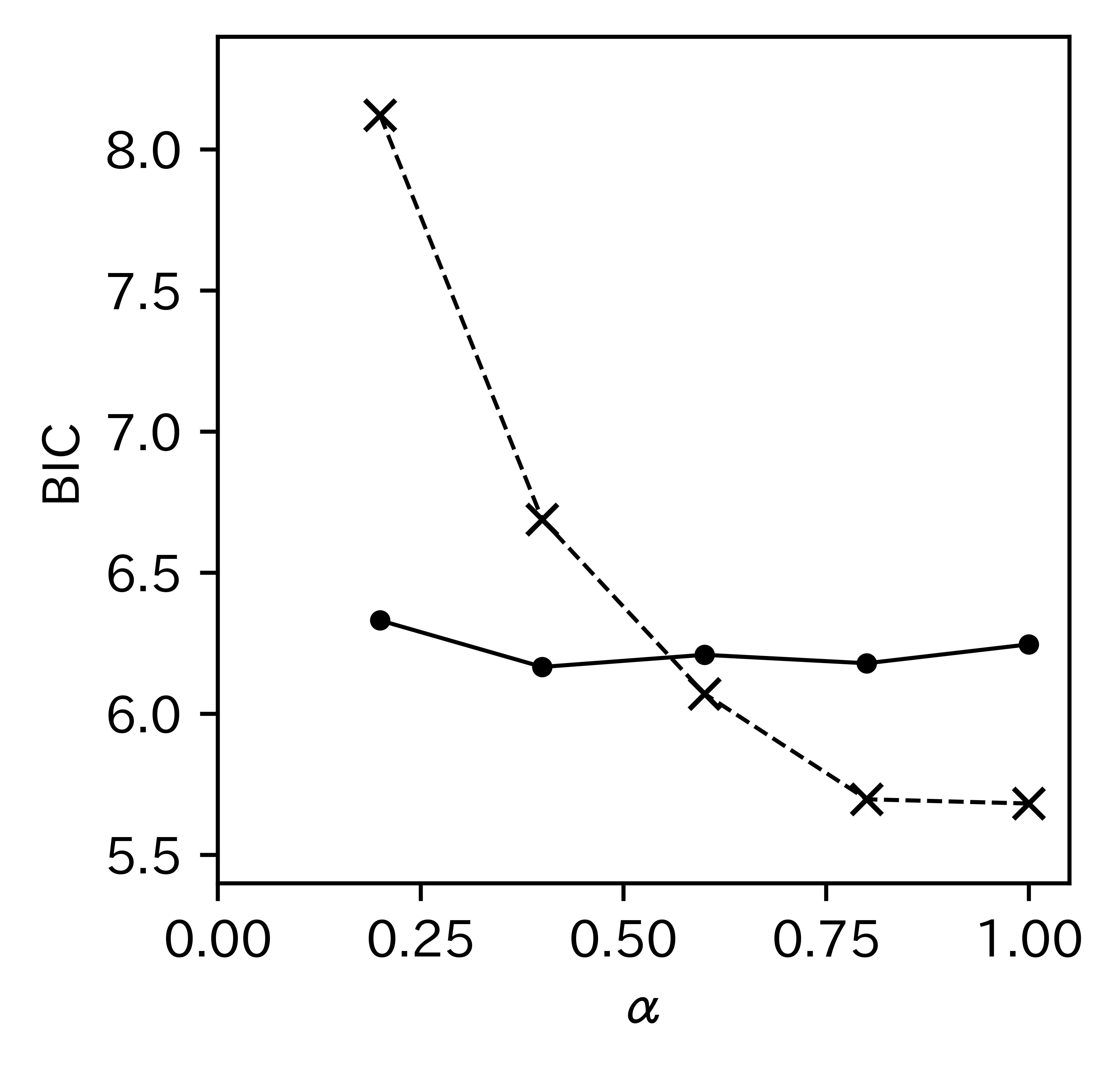
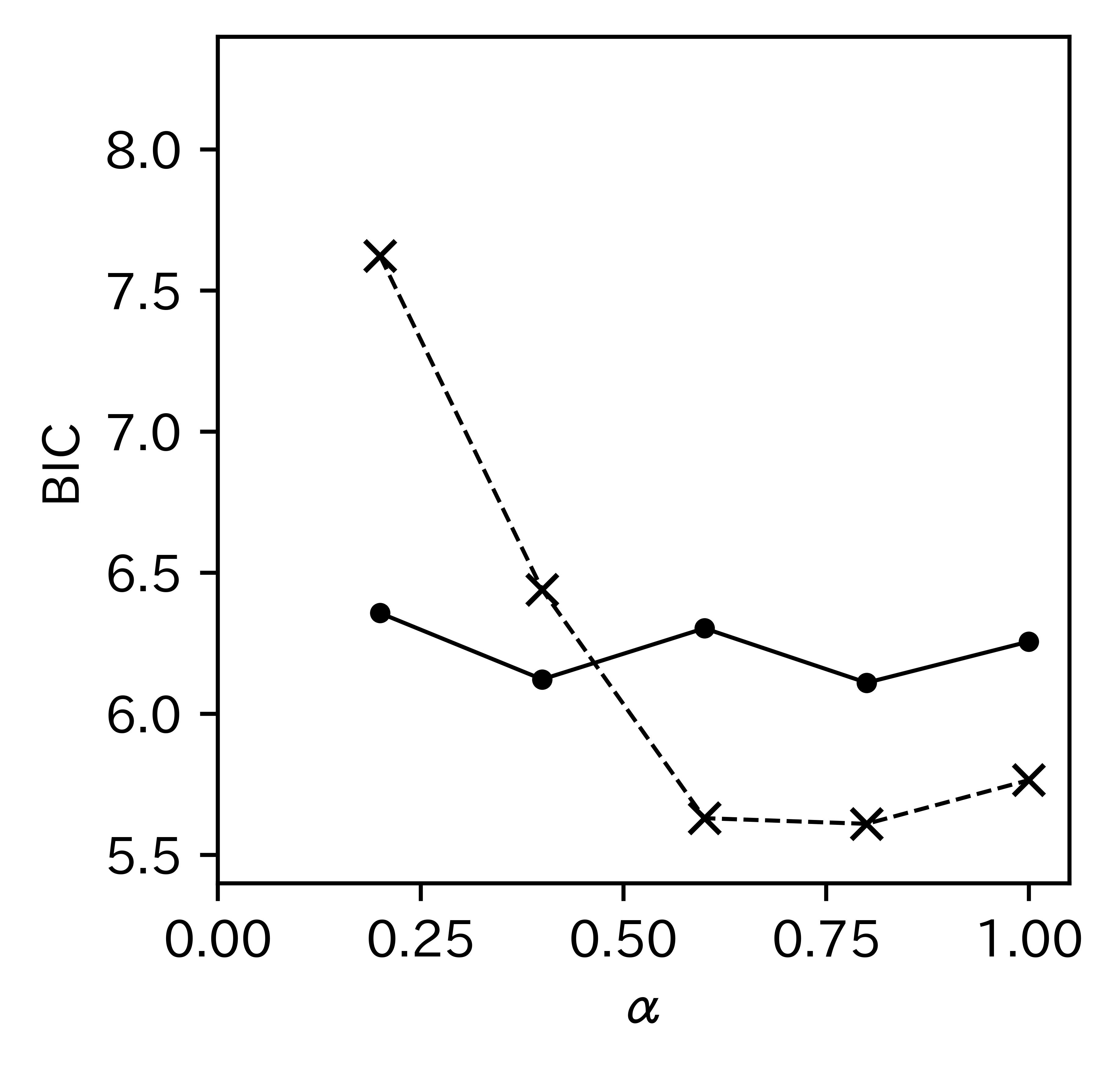
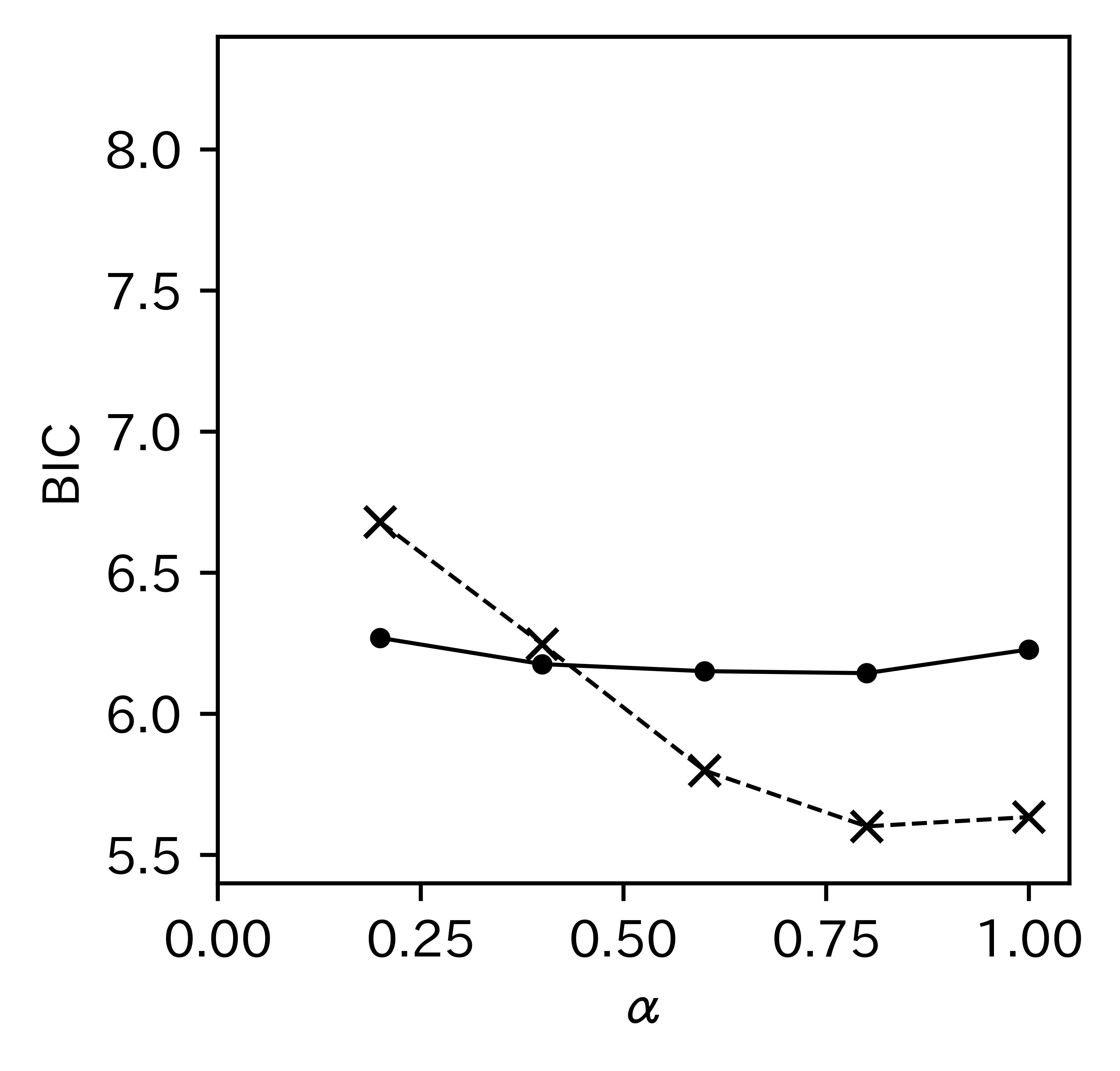
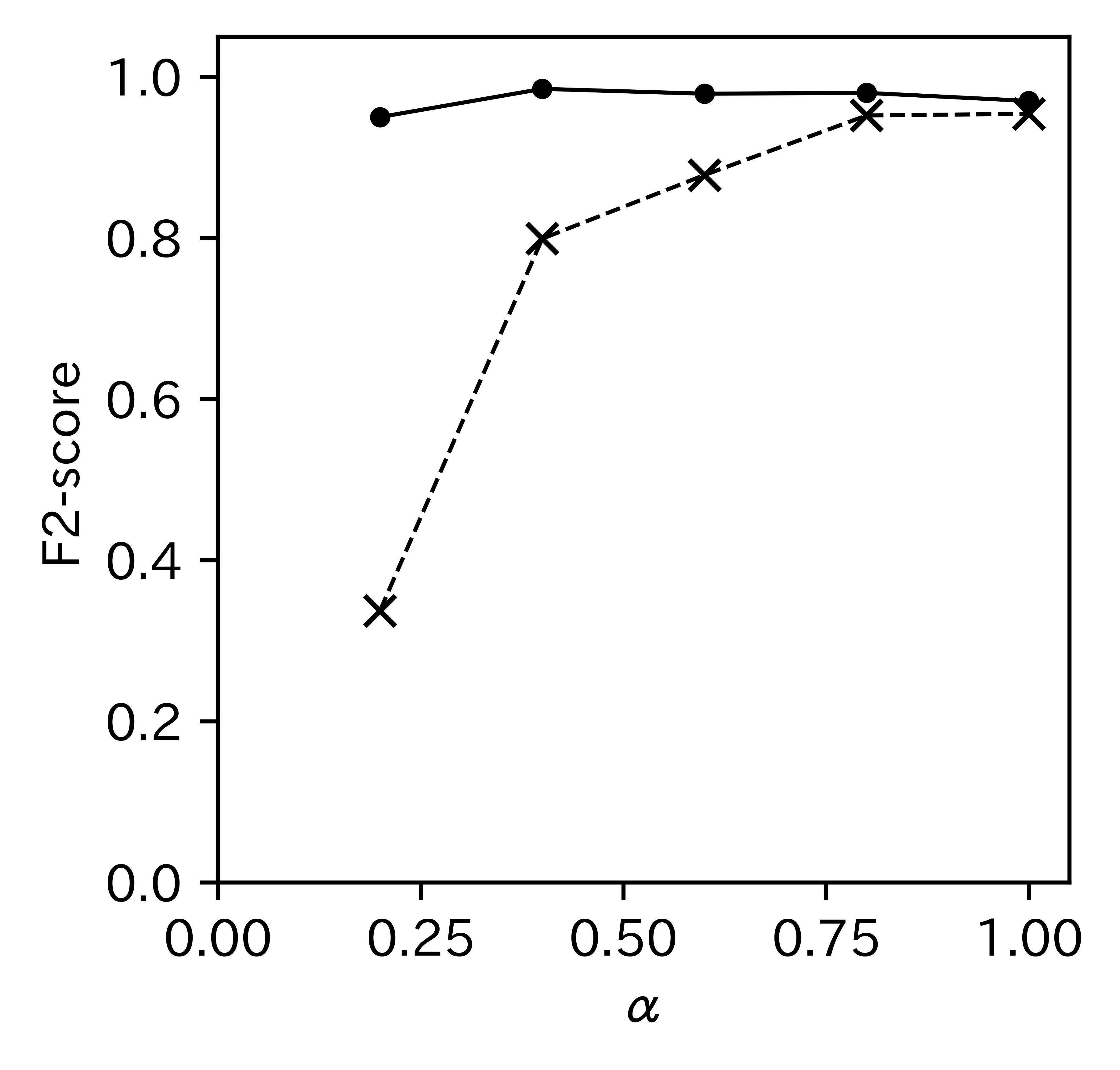
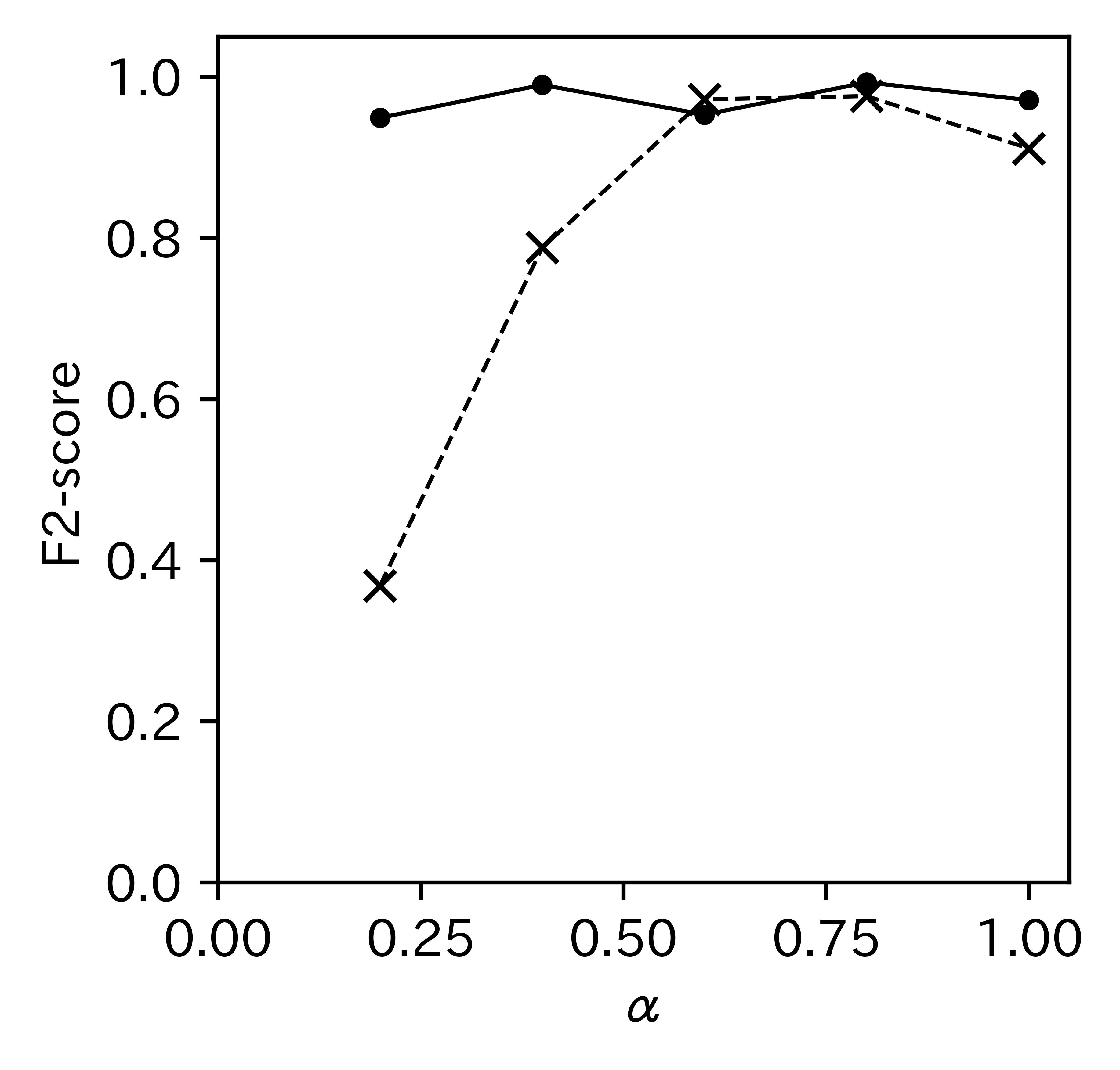
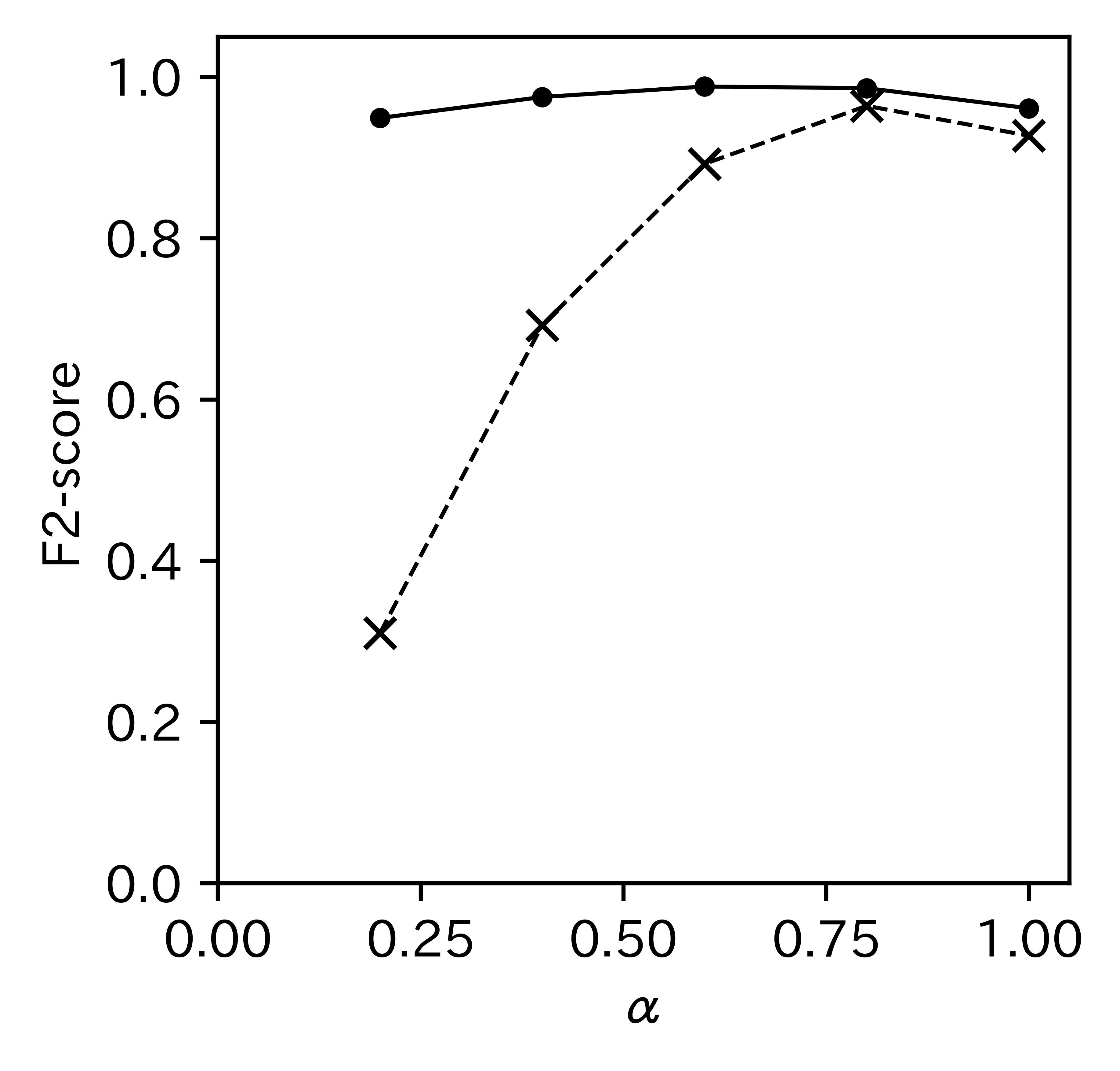
The results of the variable selection for Example 1 are shown in Table Variable screening using factor analysis for high-dimensional data with multicollinearity. The numbers in the $x_{(j)}$ column represent the total number of times that the $j$-th predictor variable is selected. For all settings, SIS never selected $x_{(4)}$. This is because $\bm{y}=(y_{1},\ldots,y_{n})^{T}$ and $(x_{14},\ldots,x_{n4})^{T}$ are uncorrelated due to the generation mechanism of the data, which gives a smaller $|\omega_{4}|$. For other methods than SIS, the value of $|\omega_{4}|$ is larger than that for SIS due to the transformation process by factor analysis. In particular, the proposed TPPIS obtains the largest $x_{(4)}$. F2-scores for TPPIS are the highest under all settings. Although the best $\alpha$ of TPPIS is 1 for the case $\varphi=0.5$, the F2-scores for TPPIS are better than those for PPIS because TPPIS selects $d$ by BIC. We confirmed that the performance of TPPIS in variable selection is improved compared to the existing methods. Figure 1 shows values of BIC and F2-scores for fixed $d$ and different $\alpha$ in TPPIS. This figure demonstrates that $\alpha$ is selected appropriately by BIC.

The results for Example 2 are shown in Table Variable screening using factor analysis for high-dimensional data with multicollinearity. The table shows that in many cases the numbers in $x_{(5)}$ are close to 100 because the fifth variable is uncorrelated with the other predictors. F2-scores for TPPIS are the highest in all cases.

Table Variable screening using factor analysis for high-dimensional data with multicollinearity summarizes the result for Example 3. This shows that the numbers in $x_{(5)}$ and the value of F2-score are smaller than those of Example 2 due to the addition of the sixth variable, which is highly correlated with the fifth variable. For the cases with $\varphi=0.9$, FPSIS_BIC and TPPIS, which determine $d$ by BIC, give lower $x_{(6)}$ values. It seems to be useful to use BIC to select $d$ for data with multicollinearity. TPPIS gives the highest F2-score among all methods.

Table Variable screening using factor analysis for high-dimensional data with multicollinearity shows the results for Example 4. In this example, the variables with large regression coefficients tend to be more important, resulting in $x_{(1)}\geq x_{(2)}\geq x_{(3)}\geq x_{(4)}$ under many settings. F2-scores for PPIS and TPPIS are high because these methods are effective for the spike model. In particular, TPPIS gives the highest F2-scores for all settings.

5 Real data analysis

We apply the proposed screening methods to the analysis of two real data sets. For both datasets, we investigated TPPIS parameters $d$ and $\alpha$, as in Section 4.1, and then the $d$ and $\alpha$ values giving the lowest BIC are selected as the optimal parameters.

5.1 Condition monitoring of hydraulic systems

We applied the screening methods to data on condition monitoring of a hydraulic system [17]. This dataset was obtained experimentally using a hydraulic test rig to measure values such as pressure, volumetric flow, and temperature while varying the settings of four different hydraulic components (coolers, valves, pumps, and accumulators). We use data with the sample size 1449, taken under stable system settings. The response is a value that expresses the degree of accumulator failure as a continuous value. A higher value is closer to normal condition with 130 being the optimal pressure, 115 being a slightly reduced pressure, 100 being a severely reduced pressure, and 90 being close to total failure. The predictors are the values measured by 17 sensors and form a total of 43680. We apply the five screening methods to analyze this dataset as in the section on examples of simulated data. The number of variables is determined using BIC.

Table Variable screening using factor analysis for high-dimensional data with multicollinearity shows the results of the analysis of this dataset. From this result we find that TPPIS selects variables from the largest number of sensors. TPPIS selects variables ‘volume flow sensors (FS)’ and ‘efficiency factor (SE)’, which are not selected by the other methods. In addition, TPPIS gives the best BIC score among all methods. These results indicate that these sensors may relate to the condition of accumulators.

5.2 S&P500

The S&P 500, one of the U.S. stock market indices, is obtained by weighting the market capitalization of 500 companies selected as representative of publicly traded companies. This analysis uses the data for the year 2020. The sample size is 253, which is the number of trading days. The response is the value of the S&P500, and the predictors are the stock price of each of the 500 companies that make up the S&P500. Note that the number of columns of predictors may be greater than 500 because some companies have multiple stocks, differentiated based on whether they include voting rights. Since the S&P500 is weighted by market capitalization, it is assumed that the stock price of the company with the highest market capitalization is selected as an important variable. The values of the S&P500 are taken from FRED [18], and the stock prices of the 500 companies that make up the S&P500 are taken from [19].

We applied five screening methods to this dataset and compared BIC and selected variables. The results for the S&P500 are shown in Table Variable screening using factor analysis for high-dimensional data with multicollinearity. TPPIS gives the best BIC score among all the methods. The 12 variables selected by TPPIS include companies with particularly large market capitalizations such as ‘AAPL’ (Apple), ‘MSFT’ (Microsoft) and ‘AMZN’ (Amazon).

6 Conclusion

We have proposed TPPIS, a variable screening method for high-dimensional data with strong multicollinearity. TPPIS improves the variable selection performance by using a BIC-type criterion to determine the number of common factors that have a role in removing multicollinearity. In the analysis of simulated data, TPPIS outperformed existing methods using factor analysis for variable selection. This suggests that TPPIS may be able to correctly select variables that are not considered important by existing methods.

The transformation process of TPPIS to remove multicollinearity from the data uses only information from the data corresponding to the predictors and we do not consider the relation to the response. Developing a transformation processing method that incorporates information from both types of data could further improve the variable selection performance. Although numerical examples confirmed that the performance of TPPIS is better than that of existing methods, no mathematical proof is provided. In the process of devising a proof, we may be able to identify the characteristics of the data for which TPPIS is most effective.

Simulation results for Example 1 $n$ $p$ $\varphi$ Method best $\alpha$ BIC F2-score $x_{(1)}$ $x_{(2)}$ $x_{(3)}$ $x_{(4)}$ 100 1000 0.5 SIS - 7.978 0.291 31 37 31 0 FPSIS - 5.778 0.930 93 93 96 91 FPSIS_BIC - 5.742 0.938 97 93 94 92 PPIS - 5.682 0.954 96 95 97 94 TPPIS 1.0 5.611 0.971 97 96 99 96 0.7 SIS - 7.612 0.258 39 28 22 0 FPSIS - 5.701 0.933 94 93 94 91 FPSIS_BIC - 5.701 0.933 94 93 94 91 PPIS - 5.765 0.911 93 92 91 88 TPPIS 0.8 5.610 0.976 99 97 98 98 0.9 SIS - 6.648 0.202 24 22 23 0 FPSIS - 5.580 0.961 96 98 96 95 FPSIS_BIC - 5.580 0.961 96 98 96 95 PPIS - 5.634 0.927 91 95 94 90 TPPIS 0.8 5.601 0.964 96 98 98 96 300 1000 0.5 SIS - 8.993 0.507 74 77 73 0 FPSIS - 6.228 0.977 100 100 100 95 FPSIS_BIC - 6.228 0.977 100 100 100 95 PPIS - 6.246 0.970 99 99 98 95 TPPIS 1.0 6.160 0.989 100 100 100 97 0.7 SIS - 8.584 0.510 75 72 77 0 FPSIS - 6.221 0.976 100 99 99 94 FPSIS_BIC - 6.158 0.980 99 98 99 97 PPIS - 6.256 0.971 98 100 98 93 TPPIS 0.8 6.110 0.993 100 100 100 99 0.9 SIS - 7.716 0.404 58 55 51 0 FPSIS - 6.195 0.969 98 98 100 93 FPSIS_BIC - 6.159 0.976 99 99 98 95 PPIS - 6.228 0.961 99 98 99 92 TPPIS 0.8 6.144 0.986 100 100 100 97

$\varphi=0.5$	$\varphi=0.7$	$\varphi=0.9$

Figure 1: Values of BIC and F2-score for different $\alpha$ in TPPIS of Example 1. The top row shows BIC results and the bottom row shows F2-score results. The values for $n=300$ are represented by $\bullet$, and the values for $n=100$ are represented by $\times$. $p$ is 1000 in all cases.

Simulation results for Example 2 $n$ $p$ $\varphi$ Method best $\alpha$ BIC F2-score $x_{(1)}$ $x_{(2)}$ $x_{(3)}$ $x_{(4)}$ $x_{(5)}$ 100 1000 0.5 SIS - 8.236 0.264 4 5 3 0 100 FPSIS - 6.336 0.921 93 93 94 93 99 FPSIS_BIC - 6.336 0.921 93 93 94 93 99 PPIS - 6.223 0.917 91 94 91 89 96 TPPIS 1.0 6.183 0.931 94 94 94 92 98 0.7 SIS - 7.726 0.245 0 2 1 0 100 FPSIS - 6.821 0.858 84 81 85 91 99 FPSIS_BIC - 6.481 0.905 90 89 94 97 100 PPIS - 6.400 0.901 92 89 95 90 96 TPPIS 1.0 6.211 0.934 95 93 96 95 99 0.9 SIS - 6.737 0.238 0 0 0 0 100 FPSIS - 7.840 0.389 21 21 28 86 35 FPSIS_BIC - 6.182 0.893 83 88 88 91 97 PPIS - 6.227 0.888 84 86 87 92 100 TPPIS 1.0 6.126 0.918 89 89 94 91 98 300 1000 0.5 SIS - 9.198 0.582 67 68 62 0 100 FPSIS - 6.422 0.970 100 98 98 93 100 FPSIS_BIC - 6.402 0.967 100 97 97 95 100 PPIS - 6.452 0.975 100 100 100 92 100 TPPIS 0.6 6.255 0.990 100 100 100 99 100 0.7 SIS - 8.774 0.484 49 51 50 0 100 FPSIS - 6.302 0.988 100 100 100 97 100 FPSIS_BIC - 6.302 0.988 100 100 100 97 100 PPIS - 6.280 0.990 100 100 100 98 100 TPPIS 1.0 6.274 0.993 100 100 100 98 100 0.9 SIS - 7.827 0.254 3 3 4 0 100 FPSIS - 6.297 0.979 99 99 99 94 100 FPSIS_BIC - 6.297 0.979 99 99 99 94 100 PPIS - 6.314 0.970 98 97 98 94 100 TPPIS 0.6 6.253 0.986 99 99 99 97 100

Simulation results for Example 3 $n$ $p$ $\varphi$ Method best $\alpha$ BIC F2-score $x_{(1)}$ $x_{(2)}$ $x_{(3)}$ $x_{(4)}$ $x_{(5)}$ $x_{(6)}$ 100 1000 0.5 SIS - 8.215 0.000 0 0 0 0 0 100 FPSIS - 6.724 0.798 86 85 86 88 80 99 FPSIS_BIC - 6.609 0.826 94 89 88 90 77 99 PPIS - 6.273 0.907 97 95 96 96 91 99 TPPIS 1.0 6.273 0.907 97 95 96 96 91 99 0.7 SIS - 7.737 0.000 0 0 0 0 0 100 FPSIS - 6.555 0.780 85 84 85 85 69 100 FPSIS_BIC - 6.468 0.837 91 89 91 93 76 100 PPIS - 6.470 0.838 91 89 90 92 81 100 TPPIS 1.0 6.274 0.887 95 94 95 96 82 99 0.9 SIS - 6.773 0.000 0 0 0 0 0 100 FPSIS - 7.220 0.401 37 31 33 93 1 97 FPSIS_BIC - 6.364 0.831 87 85 87 92 76 66 PPIS - 6.346 0.823 88 88 86 90 79 100 TPPIS 1.0 6.282 0.879 92 92 93 95 83 64 300 1000 0.5 SIS - 9.290 0.382 45 52 52 0 62 100 FPSIS - 6.510 0.923 97 97 97 94 95 100 FPSIS_BIC - 6.460 0.927 97 97 97 96 97 100 PPIS - 6.443 0.941 98 99 99 96 98 100 TPPIS 1.0 6.396 0.954 100 100 100 98 100 100 0.7 SIS - 8.845 0.217 32 32 31 0 33 100 FPSIS - 6.477 0.925 97 97 98 95 97 100 FPSIS_BIC - 6.415 0.944 99 99 99 97 99 99 PPIS - 6.379 0.950 99 99 100 98 99 100 TPPIS 1.0 6.379 0.950 99 99 100 98 99 100 0.9 SIS - 7.883 0.006 1 0 1 0 1 100 FPSIS - 6.610 0.871 95 95 95 92 95 100 FPSIS_BIC - 6.398 0.937 94 94 95 91 100 22 PPIS - 6.477 0.882 92 92 92 91 92 100 TPPIS 0.8 6.305 0.975 99 99 99 97 100 27

Simulation results for Example 4 $n$ $p$ $d$ $m$ Method best $\alpha$ BIC F2-score $x_{(1)}$ $x_{(2)}$ $x_{(3)}$ $x_{(4)}$ 100 1000 3 20 SIS - 10.595 0.332 100 5 11 0 FPSIS - 9.732 0.779 100 100 95 3 FPSIS_BIC - 9.530 0.818 100 100 90 36 PPIS - 9.432 0.836 100 100 95 33 TPPIS 1.0 9.413 0.839 100 100 92 40 40 SIS - 10.946 0.441 100 29 35 0 FPSIS - 10.329 0.771 100 100 96 0 FPSIS_BIC - 10.122 0.800 100 98 88 34 PPIS - 9.963 0.843 100 100 97 39 TPPIS 1.0 9.963 0.843 100 100 97 39 60 SIS - 11.098 0.588 100 65 61 0 FPSIS - 10.808 0.743 100 99 85 0 FPSIS_BIC - 10.808 0.743 100 99 85 0 PPIS - 10.563 0.815 100 100 96 26 TPPIS 1.0 10.563 0.815 100 100 96 26 80 SIS - 11.347 0.679 100 80 84 0 FPSIS - 11.158 0.757 100 99 91 0 FPSIS_BIC - 11.158 0.757 100 99 91 0 PPIS - 11.031 0.794 100 100 95 11 TPPIS 1.0 11.031 0.794 100 100 95 11 300 1000 3 60 SIS - 11.435 0.716 100 96 99 0 FPSIS - 11.253 0.778 100 100 100 0 FPSIS_BIC - 10.334 0.970 100 100 100 95 PPIS - 10.249 0.994 100 100 100 99 TPPIS 1.0 10.249 0.994 100 100 100 99 120 SIS - 12.240 0.773 100 100 100 0 FPSIS - 12.223 0.784 100 100 100 0 FPSIS_BIC - 11.757 0.927 100 100 100 77 PPIS - 11.688 0.948 100 100 100 85 TPPIS 1.0 11.688 0.948 100 100 100 85 180 SIS - 12.928 0.784 100 100 100 0 FPSIS - 12.918 0.788 100 100 100 0 FPSIS_BIC - 12.804 0.845 100 100 94 45 PPIS - 12.702 0.888 100 100 99 57 TPPIS 1.0 12.702 0.888 100 100 99 57 240 SIS - 13.448 0.787 100 100 100 0 FPSIS - 13.441 0.789 100 100 100 0 FPSIS_BIC - 13.441 0.789 100 100 100 0 PPIS - 13.416 0.815 100 100 92 27 TPPIS 0.8 13.408 0.823 100 100 94 30

Results for condition monitoring of hydraulic systems Method best $\alpha$ BIC Number of selected variables SIS - 6.300 12 FPSIS - 7.278 1 FPSIS_BIC - 7.027 14 PPIS - 7.051 41 TPPIS 0.4 6.271 17

Results for S&P500 Method best $\alpha$ BIC Number of selected variables SIS - 2.118 2 FPSIS - 1.986 5 FPSIS_BIC - 1.387 12 PPIS - 1.818 11 TPPIS 0.4 1.101 7

References

- [1] Tian S, Yu Y, Guo H. Variable selection and corporate bankruptcy forecasts. J Bank Financ. 2015;52:89–100.
- [2] Fang T, Lee TH, Su Z. Predicting the long-term stock market volatility: A garch-midas model with variable selection. J Empir Finance. 2020;58:36–49.
- [3] Chowdhury MZI, Turin TC. Variable selection strategies and its importance in clinical prediction modelling. Fam Med Community Health. 2020;8(1).
- [4] Yun YH, Li HD, Deng BC, et al. An overview of variable selection methods in multivariate analysis of near-infrared spectra. Trends Analyt Chem. 2019;113:102–115.
- [5] Fan J, Lv J. Sure independence screening for ultrahigh dimensional feature space. J R Stat Soc B. 2008;70(5):849–911.
- [6] Fan J, Song R. Sure independence screening in generalized linear models with np-dimensionality. 2010;.
- [7] Fan J, Feng Y, Song R. Nonparametric independence screening in sparse ultra-high-dimensional additive models. J Am Stat Assoc. 2011;106(494):544–557.
- [8] Li G, Peng H, Zhang J, et al. Robust rank correlation based screening. 2012;.
- [9] Li R, Zhong W, Zhu L. Feature screening via distance correlation learning. J Am Stat Assoc. 2012;107(499):1129–1139.
- [10] Balasubramanian K, Sriperumbudur B, Lebanon G. Ultrahigh dimensional feature screening via rkhs embeddings. In: Proceedings of the Sixteenth International Conference on Artificial Intelligence and Statistics; 2013 29 April- 1 May; Scottsdale, Arizona. PMLR; 2013. p. 126–134.
- [11] Zhang J, Liu Y, Wu Y. Correlation rank screening for ultrahigh-dimensional survival data. Comput Statist Data Anal. 2017;108:121–132.
- [12] Fan J, Lv J. Sure independence screening. Wiley StatsRef: Stat Ref Online. 2018;.
- [13] Wang X, Leng C. High dimensional ordinary least squares projection for screening variables. J R Stat Soc B. 2016;:589–611.
- [14] Wang H. Factor profiled sure independence screening. Biometrika. 2012;99(1):15–28.
- [15] Zhao N, Xu Q, Tang ML, et al. High-dimensional variable screening under multicollinearity. Stat. 2020;9(1):e272.
- [16] Jia J, Rohe K. Preconditioning to comply with the irrepresentable condition. arXiv preprint arXiv:12085584. 2012;.
- [17] Helwig N, Pignanelli E, Schütze A. Condition monitoring of a complex hydraulic system using multivariate statistics. In: 2015 IEEE International Instrumentation and Measurement Technology Conference (I2MTC) Proceedings; 2015 11-14 May; Pisa, Italy. IEEE; 2015. p. 210–215.
- [18] FRED [Internet]. St. Louis: Federal Reserve Bank of St. Louis ; 2023 Jan 25 [cited 2023 Jan 25]. Available from: https://fred.stlouisfed.org/series/SP500.
- [19] Hanseo P. Data from: S&P 500 stocks price with financial statement [dataset] ; 2022 Apr 18 [cited 2023 Jan 25]. In: Kaggle Datasets [Internet]. Available from: https://www.kaggle.com/hanseopark/sp-500-stocks-value-with-financial-statement.
Simulation results for Example 1 Method best BIC F2-score 100 1000 0.5 SIS - 7.978 0.291 31 37 31 0 FPSIS - 5.778 0.930 93 93 96 91 FPSISBIC - 5.742 0.938 97 93 94 92 PPIS - 5.682 0.954 96 95 97 94 TPPIS 1.0 5.611 0.971 97 96 99 96 0.7 SIS - 7.612 0.258 39 28 22 0 FPSIS - 5.701 0.933 94 93 94 91 FPSISBIC - 5.701 0.933 94 93 94 91 PPIS - 5.765 0.911 93 92 91 88 TPPIS 0.8 5.610 0.976 99 97 98 98 0.9 SIS - 6.648 0.202 24 22 23 0 FPSIS - 5.580 0.961 96 98 96 95 FPSISBIC - 5.580 0.961 96 98 96 95 PPIS - 5.634 0.927 91 95 94 90 TPPIS 0.8 5.601 0.964 96 98 98 96 300 1000 0.5 SIS - 8.993 0.507 74 77 73 0 FPSIS - 6.228 0.977 100 100 100 95 FPSISBIC - 6.228 0.977 100 100 100 95 PPIS - 6.246 0.970 99 99 98 95 TPPIS 1.0 6.160 0.989 100 100 100 97 0.7 SIS - 8.584 0.510 75 72 77 0 FPSIS - 6.221 0.976 100 99 99 94 FPSISBIC - 6.158 0.980 99 98 99 97 PPIS - 6.256 0.971 98 100 98 93 TPPIS 0.8 6.110 0.993 100 100 100 99 0.9 SIS - 7.716 0.404 58 55 51 0 FPSIS - 6.195 0.969 98 98 100 93 FPSISBIC - 6.159 0.976 99 99 98 95 PPIS - 6.228 0.961 99 98 99 92 TPPIS 0.8 6.144 0.986 100 100 100 97