Bayes optimal learning in high-dimensional linear regression with network side information

Abstract

Supervised learning problems with side information in the form of a network arise frequently in applications in genomics, proteomics and neuroscience. For example, in genetic applications, the network side information can accurately capture background biological information on the intricate relations among the relevant genes. In this paper, we initiate a study of Bayes optimal learning in high-dimensional linear regression with network side information. To this end, we first introduce a simple generative model (called the Reg-Graph model) which posits a joint distribution for the supervised data and the observed network through a common set of latent parameters. Next, we introduce an iterative algorithm based on Approximate Message Passing (AMP) which is provably Bayes optimal under very general conditions. In addition, we characterize the limiting mutual information between the latent signal and the data observed, and thus precisely quantify the statistical impact of the network side information. Finally, supporting numerical experiments suggest that the introduced algorithm has excellent performance in finite samples.

1 Introduction

Given data $\{(y_{i},\phi_{i}):1\leq i\leq n\}$, $y_{i}\in\mathbb{R}$, $\phi_{i}\in\mathbb{R}^{p}$, the classical linear model

$$\mathbf{y}=\mathbf{\Phi}\mathbb{\beta}+\varepsilon.$$ (1.1)

furnishes an ideal test bed to study the performance of diverse supervised learning algorithms. In the modern age of big data, the number of observations $n$ and the feature dimension $p$ are often both large and comparable.

In these challenging high-dimensional scenarios, scientists have recognized the importance of incorporating domain knowledge into the relevant statistical inference methodology. Success in this direction can substantially boost the performance of statistical procedures, and facilitate novel discoveries in critical applications. Arguably, the most well-known instance of this philosophy is the incorporation of sparsity into high-dimensional statistical methods (see e.g. [66, 21, 57, 39]).

In this paper, we consider a setting where in addition to the supervised data, one observes pairwise relations among the features in the dataset. This pairwise relation can be conveniently captured using a graph $\mathbf{G}=(V,E)$. The vertices in the graph represent the features. The edges represent pairwise relations among the features e.g., an edge might indicate that the two endpoints are likely to be both included in the support of the linear model.

This setup is motivated by datasets arising in diverse application areas e.g., genomics, proteomics and neuroscience. In the genomic context, the response $y$ represents phenotypic measurements on an individual, while the features $\phi$ represent genetic expression. In addition, scientists often have background knowledge about genetic co-expressions—this information can be efficiently captured in terms of the graph described above. We refer the interested reader to [44, 42] for detailed discussions of settings where such data sets arise naturally. To study this problem in depth, we first introduce a simple generative model, which we refer to as the Reg-Graph model.

• Generate $\sigma_{1},\cdots,\sigma_{p}\stackrel{{\scriptstyle i.i.d.}}{{\sim}}\mbox{Bernoulli}(\rho)$ for some $\rho$ in $(0,1)$.

• Given $\mathbf{\sigma}=(\sigma_{1},\cdots,\sigma_{p})$, generate regression coefficients $\beta_{i}|\sigma_{i}\sim P(\cdot|\sigma_{i})$, where $P(\cdot|\cdot)$ is a Markov kernel. Throughout, we assume that $P(\cdot|0)$ and $P(\cdot|1)$ have finite second moments.

• Given the regression coefficients $\mathbf{\beta}=(\beta_{1},\cdots,\beta_{p})$ and features $\phi_{\mu}\in\mathbb{R}^{p}$, $1\leq\mu\leq n$, the response $y$ is sampled using a linear model

  $$y_{\mu}=\sum_{i=1}^{p}\beta_{0i}\phi_{\mu i}+\varepsilon_{\mu},$$ (1.2)

  where $\varepsilon_{\mu}\sim N(0,\Delta)$ are i.i.d.

• Finally, one observes a graph $\mathbf{G}=(V,E)$ on $p$ vertices. As mentioned above, the vertices represent the observed features. We assume that given $\sigma_{1},\cdots,\sigma_{p}$, the edges are added independently with probability

  $$\mathbb{P}[\{i,j\}\in E|\sigma_{1},\cdots,\sigma_{p}]=\begin{cases}\frac{a_{p}}{p}&\textrm{if}\,\,\,\sigma_{i}\sigma_{j}=1\\ \frac{b_{p}}{p}&\textrm{o.w.}\end{cases}$$ (1.3)

  In this formulation, $\{a_{p}:p\geq 1\}$ and $\{b_{p}:p\geq 1\}$ represent general sequences dependent on $p$.

We note that our Reg-Graph model ties the generation of the regression data and the graph $\mathbf{G}$ via the same underlying variables $\sigma_{1},\cdots,\sigma_{p}$. In this context, one naturally wishes to combine the two data sources to carry out inference on these common latent parameters. Throughout, we assume that the model parameters $\rho$, $P(\cdot|\cdot)$, $\Delta$, $a_{p},b_{p}$ are known to the statistician.

The Reg-Graph model naturally ties together some popular ideas in statistics and machine learning:

• Note that the marginal distribution of the supervised data $\{(y_{\mu},\phi_{\mu}):1\leq\mu\leq n\}$ includes the celebrated spike and slab model from Bayesian statistics [39]. For the spike and slab model, one assumes in addition that $P(\cdot|0)=\delta_{0}$. Informally, the sigma variables encode the support of the signal vector $\beta$ in this case, and one wishes to recover the latent indicators $\sigma_{i}$ from the data. The spike and slab model and its relatives have emerged as the canonical choice for sparse regression models in high-dimensional Bayesian statistics in the past two decades (we refer the interested reader to [65] and the references therein for a detailed survey of the progress in this area). While this is not necessary for our model, we will explore this case in depth in our subsequent discussion.

• On the other hand, if we focus on the marginal distribution of the graph $\mathbf{G}$, it corresponds to a graph with a hidden community [34, 3, 33]. In this case, one typically assumes that $a_{p}\geq b_{p}$, so that the vertices with $\sigma_{i}=1$ have a higher density of connecting edges. The recovery of the hidden community from the graph data has been studied in-depth in the recent past [51].

Thus the Reg-Graph model ties together two distinct threads of enquiry in statistics and machine learning using a natural generative model. We note that the one hidden community assumption is a convenient simplification—the model and our subsequent results can be naturally extended to a setting with multiple latent communities.

In this paper, we study the Reg-Graph model, and make the following contributions:

• We study the Reg-Graph model under an additional i.i.d. gaussian assumption on the features $\phi_{\mu}$. In addition, we assume a proportional asymptotic setting, where the number of observations $n$ and the feature dimension $p$ are both large and comparable. Formally, we assume that $n/p\to\kappa\in(0,\infty)$. Note that we allow $\kappa\in(0,1)$, and thus can cover settings where the feature dimension $p$ is larger than the sample size $n$. Under these assumptions, we introduce an algorithm based on Approximate Message Passing (AMP) [11, 29] for estimation (of $\beta_{0}$) and support recovery (i.e., recovery of $\sigma_{0}$). We characterize the precise $L^{2}$-estimation error and the limiting False Discovery Proportion (FDP) under this algorithm.

• We characterize the mutual information between the data and the latent parameters under the Reg-Graph model. In particular, this allows us to derive the Bayes optimal estimation error in this setting. We establish that under a wide class of priors, the AMP algorithm introduced in the previous step is Bayes optimal.

  To derive the limiting mutual information in this model, we use the adaptive interpolation method developed by Barbier and Macris, 2019a [7]. This approach has been used in several past works to characterize the limiting mutual information in planted models (see e.g. [6] and references therein), and we build directly on these seminal works. We note that the mutual information in high-dimensional models can also be derived using other techniques (see e.g. [58, 5, 9])—the mutual information in our setting can also be potentially characterized by adopting these alternative approaches.

• Finally, using numerical simulations, we compare the statistical performance of the proposed AMP algorithm with existing penalization based approaches for estimation and support recovery. In our numerical experiments, the AMP algorithm significantly outperforms the benchmark algorithm.

1.1 Main Results

We highlight our main results in this section.

1.1.1 Algorithm based on Approximate Message Passing

As a first step, we introduce a class of iterative algorithms based on Approximate Message Passing (AMP) for parameter estimation and support recovery in the Reg-Graph model. This algorithm naturally incorporates the supervised data with the auxiliary graph information for statistical inference. To this end, we set $\bm{S}=\bm{\Phi}/\sqrt{\kappa}$ and $\widebar{\bm{A}}=(\bm{A}-b_{p})/\sqrt{b_{p}(1-b_{p})}$, where $\mathbf{A}$ denotes the adjacency matrix of the graph $\mathbf{G}$. Set $\bm{y}^{\circ}=\bm{y}/\sqrt{\kappa}$.

Formally, Approximate Message Passing is not a single algorithm, but rather a class of iterative algorithms, which are specified in terms of a sequence of non-linearities used in each step. We refer the interested reader to [11, 29] for a discussion on the origins of AMP and its applications to high-dimensional statistics and signal processing. To describe the specific instance of AMP we use in our setting, consider two sequences of Lipschitz functions $\zeta_{t}:\mathbb{R}^{2}\rightarrow\mathbb{R}$, $f_{t}:\mathbb{R}^{2}\rightarrow\mathbb{R}$, with Lipschitz derivatives and the synchronized approximate message passing orbits $\{\bm{\sigma}^{t+1}\}_{t\geq 0}$ and $\{\bm{z}^{t},\bm{\beta}^{t+1}\}_{t\geq 0}$ defined as follows.

$$\bm{\sigma}^{t+1} =\frac{\widebar{\bm{A}}}{\sqrt{p}}\bm{f}_{t}(\bm{\sigma}^{t},\bm{S}^{\top}\bm{z}^{t-1}+\bm{\beta}^{t-1})$$ (1.4)

$$\quad\quad-(\mathcal{A}\bm{f}_{t})(\bm{\sigma}^{t},\bm{S}^{\top}\bm{z}^{t-1}+\bm{\beta}^{t-1})\bm{f}_{t-1}(\bm{\sigma}^{t-1},\bm{S}^{\top}\bm{z}^{t-2}+\bm{\beta}^{t-2}),$$ (1.5)

$$\bm{z}^{t} =\bm{y}^{\circ}-\bm{S}\bm{\beta}^{t}+\frac{1}{\kappa}\bm{z}^{t-1}(\mathcal{A}\bm{\zeta}_{t-1})(\bm{S}^{\top}\bm{z}^{t-1}+\bm{\beta}^{t-1},\bm{\sigma}^{t})$$ (1.6)

$$\bm{\beta}^{t+1} =\bm{\zeta}_{t}(\bm{S}^{\top}\bm{z}^{t}+\bm{\beta}^{t},\bm{\sigma}^{t+1})$$ (1.7)

where the functions $\bm{\zeta}_{t}:(\mathbb{R}^{2})^{p}\rightarrow\mathbb{R}^{p}$, $\bm{f}_{t}:(\mathbb{R}^{2})^{p}\rightarrow\mathbb{R}^{p}$ are defined as $\bm{\zeta}_{t}(\bm{x}):=(\zeta_{t}(\bm{x}_{1}),\cdots,\zeta_{p}(\bm{x}_{p}))$ and $\bm{f}_{t}(\bm{x}):=(f_{t}(\bm{x}_{1}),\cdots,f_{p}(\bm{x}_{p}))$. Finally, for a function $\bm{g}:(\mathbb{R}^{s})^{k}\rightarrow\mathbb{R}^{s}$, $(\mathcal{A}\bm{g})(\bm{t})$ is defined as $(\mathcal{A}\bm{g})(\bm{t})=\frac{1}{k}\sum\limits_{i=1}^{k}\frac{\partial}{\partial t}g(\bm{t}_{i}).$ Here, the derivative is with respect to the first argument if there are multiple arguments to the function.

The performance of the AMP algorithms described above will be characterized in terms of some low-dimensional scalar parameters [11]. In turn, these scalar parameters are defined using an iteration referred to as state evolution. Formally, define the parameters $\tau^{2}_{t}$, $\sigma^{2}_{t}$, $\nu^{2}_{t}$ and $\mu_{t}$ by the following iteration.

$$\tau^{2}_{t} =\frac{1}{\kappa}\left(\Delta+\,\mathbb{E}[(\zeta_{t-1}(B+\tau_{t-1}Z_{1},\eta_{t}\Sigma+\nu_{t}Z_{2})-B)^{2}]\right),$$ (1.8)

$$\nu^{2}_{t+1} =\mathbb{E}[f^{2}_{t}(B+\tau_{t-1}Z_{1},\eta_{t}\Sigma+\nu_{t}Z_{2})],$$ (1.9)

$$\eta_{t+1} =\sqrt{\lambda}\nu^{2}_{t+1},$$ (1.10)

where $Z_{1},Z_{2},Z_{3}$ are i.i.d $\mathsf{N}(0,1)$, $\Sigma\sim\mathsf{Bernoulli}(\rho)$, $B|\Sigma\sim P(\cdot|\Sigma)$, $W\sim\mathsf{N}(0,\Delta/\kappa)$ and the initial conditions are given by $\tau^{2}_{0}=\frac{1}{\kappa}\left(\Delta+\,\mathbb{E}[B^{2}]\right)\quad\mbox{and}\quad\tau_{-1}=\eta_{0}=\nu_{0}=0$. We will consider a specific sequence of update functions, given as $f_{-1}=0$ and for $t\geq 1$,

$$f_{t}(x,y) :=\mathbb{E}[\Sigma|B+\tau_{t-1}Z_{1}=x,\eta_{t}\Sigma+\nu_{t}Z_{2}=y],$$

$$\zeta_{t-1}(x,y) :=\mathbb{E}[B|B+\tau_{t-1}Z_{1}=x,\eta_{t}\Sigma+\nu_{t}Z_{2}=y].$$

Using this specific sequence of non-linearities in (1.5),(1.7) we obtain the sequence of estimates given by $\widehat{\bm{\sigma}}^{t}=\bm{f}_{t-1}(\Phi^{\top}\bm{z}^{t}+\bm{\beta}^{t},\bm{\sigma}^{t})$ and $\widehat{\bm{\beta}}^{t}=\bm{\beta}^{t}$. One obtains valid estimates for each $t\geq 1$. Typically, the statistical performance improves with increasing number of iterations. To quantify the limiting statistical performance of the estimators obtained (in the limit of a large number of iterations), we introduce

$$\mathsf{MSE^{AMP}_{\sigma}}:=\lim\limits_{t\rightarrow\infty}\lim\limits_{p\rightarrow\infty}\frac{1}{p^{2}}\;\mathbb{E}[\|\widehat{\bm{\sigma}}^{t}(\widehat{\bm{\sigma}}^{t})^{\top}-\bm{\sigma}\bm{\sigma}^{\top}\|^{2}],\,\,\mathsf{MSE^{AMP}_{\beta}}:=\lim\limits_{t\rightarrow\infty}\lim\limits_{n\rightarrow\infty}\frac{1}{n}\;\mathbb{E}[\|\bm{\Phi}(\widehat{\bm{\beta}}^{t}-\bm{\beta}_{0})\|^{2}].$$

Note the specific order of the iterated limits—we let the dimension $p\to\infty$ before we let the number of iterations diverge. This order of iterated limits is typical in the analysis of AMP algorithms. Using recent progress in the analysis of AMP algorithms, it might be possible to analyze the AMP algorithms after a slowly growing number of steps [45, 61, 17], but we refrain from examining this direction in this paper.

To characterize the limiting behavior of $\mathsf{MSE^{AMP}_{\sigma}}$ and $\mathsf{MSE^{AMP}_{\beta}}$, we need to introduce one final set of scalar functionals. Define

$$\mathsf{mmse}_{1}(\mu,\xi)=\mathbb{E}\left\{\Sigma-\mathbb{E}\Bigg{[}\Sigma|B+\sqrt{(\Delta(1+\xi)/\kappa)}Z_{1},\sqrt{\mu}\Sigma+Z_{2}\right]\Bigg{\}}^{2},$$ (1.11)

$$\mathsf{mmse}_{2}(\mu,\xi):=\mathbb{E}\left\{B-\mathbb{E}\Bigg{[}B|B+\sqrt{(\Delta(1+\xi)/\kappa)}Z_{1},\sqrt{\mu}\Sigma+Z_{2}\right]\Bigg{\}}^{2}.$$ (1.12)

Armed with this definition, we can write

$$\mathbb{E}\left[\mathbb{E}\left[\Sigma|B+\sqrt{(\Delta(1+\xi)/\kappa)}Z_{1},\sqrt{\mu}\Sigma+Z_{2}\right]^{2}\right]=\rho-\mathsf{mmse}_{1}(\mu,\xi).$$

The next result characterizes the limiting statistical behavior of the AMP algorithm.

Theorem 1.1.

Assume that $\frac{b_{p}}{p}(1-\frac{b_{p}}{p})\geq C\,\frac{\log p}{p}$ for any constant $C>0$. Then we have

$$\mathsf{MSE^{AMP}_{\sigma}}=\rho^{2}-\frac{(\mu^{*})^{2}}{\lambda^{2}},\,\,\,\,\,\mathsf{MSE^{AMP}_{\beta}}=\frac{\Delta\;\xi^{*}}{(1+\xi^{*})},$$ (1.13)

where $(\mu^{*},\xi^{*})$ satisfy the following fixed point equations.

$$\mu^{*}=\lambda(\rho-\mathsf{mmse}_{1}(\mu^{*},\xi^{*})),\,\,\,\,\xi^{*}=\frac{1}{\Delta}\mathsf{mmse}_{2}(\mu^{*},\xi^{*}).$$ (1.14)

Remark 1.1.

We note here that the system of equations (1.14) could have multiple solutions in general.

Remark 1.2.

We analyze the AMP algorithm introduced above using the results of [49]. However, we remark that the algorithm can be equivalently analyzed using the powerful general framework introduced in [30]. To the best of our knowledge, AMP algorithms with such interacting sets of variables arose originally in [50] in the analysis of multi-layer generalized linear estimation problems.

1.1.2 Statistical Optimality of the Algorithm

Having introduced an algorithm based on Approximate Message Passing, we turn to the question of optimal statistical estimation in this setting. In this section, we identify a broad class of settings where the AMP based algorithm introduced above yields optimal statistical performance.

As a first step, we characterize the limiting mutual information between the underlying signal $(\bm{\beta}_{0},\bm{\sigma})$ and the observed data. In addition to being a fundamental information theoretic object in its own right, the limiting mutual information will help us characterize the estimation performance of the Bayes optimal estimator in this setup.

To this end, we assume that the conditional distributions $P(\cdot|0)$ and $P(\cdot|1)$ have finite supports contained in some compact interval $[-s_{\max},s_{\max}]$. This finite support assumption is merely for technical convenience—we expect that the results can be extended to unbounded, light tailed (e.g. subgaussian) settings with additional work. Note that the special case $P(\cdot|0)=\delta_{0}$ corresponds to a discrete case of the classical spike and slab prior. Recall that the mutual information between $(\bm{\beta}_{0},\bm{\sigma})$ and the data represented by $(\bm{A},\bm{\Phi},\bm{y})$ is defined as follows:

$$I(\bm{\beta}_{0},\bm{\sigma};\bm{A},\bm{\Phi},\bm{y})=\mathbb{E}_{(\bm{\beta}_{0},\bm{\sigma},\bm{\Phi})}\left[\log\frac{P(\bm{A},\bm{y}|\bm{\beta}_{0},\bm{\sigma})}{P(\bm{A},\bm{y})}\right].$$

Define

$$y:=\sqrt{\mu}\Sigma+\widebar{Z}\quad\mbox{and}\quad a:=B+\sqrt{\frac{\Delta(1+\xi)}{\kappa}}\widebar{\varepsilon},$$

where $\Sigma\sim\mathsf{Bernoulli}(\rho)$, $B|\Sigma\sim P(\cdot|\Sigma)$ and $\widebar{Z},\widebar{\varepsilon}\sim\mathsf{N}(0,1)$. Finally, $\Sigma,B,\widebar{Z}$ and $\widebar{\varepsilon}$ are independent. We further set

$$\mathsf{I}(\mu,\xi;\Delta):=\mathbb{E}\left[\log\frac{P(y,a|\Sigma,B)}{P(y,a)}\right].$$

Then we have the following theorem characterizing the limiting mutual information.

Theorem 1.2.

If $b_{p}(1-\frac{b_{p}}{p})\rightarrow\infty$ as $n,p\rightarrow\infty$, then we have

$$\mathcal{I}:=\lim\limits_{p\rightarrow\infty}\frac{1}{p}I(\bm{\beta}_{0},\bm{\sigma};\bm{A},\bm{\Phi},\bm{y})$$

$$=\min\limits_{\mu,\xi\geq 0}\Bigg{\{}\frac{\lambda\rho^{2}}{4}+\frac{\mu^{2}}{4\lambda}+\frac{\kappa}{2}\left[\log\left(1+\xi\right)-\frac{\xi}{1+\xi}\right]-\frac{\mu\rho}{2}+\mathsf{I}(\mu,\xi;\Delta)\Bigg{\}}.$$ (1.15)

Observe that if $(\widebar{\mu},\widebar{\xi})$ is the global optimizer of the RHS of (1.2), the first order stationary point conditions imply that $(\widebar{\mu},\widebar{\xi})$ satisfy the fixed point equations

$$\widebar{\mu} =\lambda(\rho-\mathsf{mmse}_{1}(\widebar{\mu},\widebar{\xi})),$$ (1.16)

$$\widebar{\xi} =\frac{1}{\Delta}\mathsf{mmse}_{2}(\widebar{\mu},\widebar{\xi}).$$ (1.17)

Recalling (1.18), we see that $(\mu^{*},\xi^{*})$ satisfy the same fixed point system. Of course, the fixed point system can have multiple solutions, and thus these two solutions are not equal in general.

Our next result establishes that if these fixed points actually coincide, then the AMP based algorithm has Bayes optimal reconstruction performance. To this end, define

$$\mathsf{MMSE}=\frac{1}{p^{2}}\mathbb{E}[\|\bm{\sigma}\bm{\sigma}^{\top}-\mathbb{E}[\bm{\sigma}\bm{\sigma}^{\top}|\bm{A},\bm{y},\bm{\Phi}]\|^{2}],\,\,\,\mathsf{y}_{\mathrm{mmse}}:=\frac{1}{n}\mathbb{E}[\|\bm{\Phi}(\mathbb{E}[\bm{\beta}|\bm{A},\bm{y},\bm{\Phi}]-\bm{\beta}_{0})\|^{2}_{2}].$$ (1.18)

Note that $\mathsf{MMSE}$ and $\mathsf{y}_{\mathrm{mmse}}$ captures the reconstruction performance of the Bayes optimal estimators in this setting.

Theorem 1.3.

Assume that $(\mu^{*},\xi^{*})=(\widebar{\mu},\widebar{\xi})$. Then we have

$$\lim\limits_{p\rightarrow\infty}\mathsf{MMSE}=\mathsf{MSE^{AMP}_{\sigma}}\quad\mbox{and}\quad\lim\limits_{p\rightarrow\infty}\mathsf{y_{mmse}}=\mathsf{MSE^{AMP}_{\beta}}.$$

In general, it is hard to check the Assumption in Theorem  1.3. If (1.18) has a unique root, the assumption is trivially satisfied—indeed, this is one prominent example when the above condition can be verified in practice. A difference between $(\mu^{*},\xi^{*})$ and $(\widebar{\mu},\widebar{\xi})$ is naturally associated with potential statistical/computational gaps in this problem. We defer a discussion of this point to Section 4.

1.1.3 Variable discovery and applications to multiple testing

We turn to the recovery of non-null variables in this section. We will work under the Reg-Graph model, and assume that $P(\cdot|\sigma_{i})=\delta_{0}\,\mathbb{I}(\sigma_{i}=0)+\mathrm{Q}\,\mathbb{I}(\sigma_{i}=1)$, $\mathrm{Q}((-\varepsilon,\varepsilon))=0$ for some $\varepsilon>0$. In this case, discovering the non-null variables is equivalent to recovering the non-zero $\sigma_{i}$ variables. Specifically, we consider the hypothesis tests

$$H_{0i}:\sigma_{i}=0\quad\mbox{vs}\quad H_{0i}:\sigma_{i}\neq 0.$$

To develop a multiple testing procedure for this setting, we will employ the Bayes optimal AMP algorithm (1.5), (1.7). Our algorithm is inspired by a similar strategy developed in [52] in the context of a low rank matrix recovery problem. We use the $\sigma^{t}$ iterates to devise a Benjamini-Hochberg type multiple testing procedure for variable discovery. Recall the state evolution parameters $\tau^{2}_{t},\nu^{2}_{t}$ and $\eta_{t}$’s defined by (1.8). Consider the following p-values to test the hypotheses stated above.

$$p_{i}=2\,\left(1-\Phi\left(\frac{|\sigma^{t}_{i}|}{\nu_{t}}\right)\right).$$ (1.19)

Our next result establishes that the p-values introduced above are actually asymptotically valid.

Theorem 1.4.

Consider the $P$-values defined by (1.19). Then, if $\sigma_{i_{0}}=0$, for any $\alpha\in[0,1]$,

$$\lim\limits_{n\rightarrow\infty}\mathbb{P}\left[p_{i_{0}}(t)\leq\alpha\right]=\alpha.$$

Using these p-values we shall design a Benjamini-Hochberg type procedure (Benjamini and Hochberg, [14]) for variable selection, which controls the false discovery proportion at level $\alpha$. To this end, we define the following estimator of false discovery proportion:

$$\widehat{\mathrm{FDP}}(s;t):=\frac{n(1-\rho)s}{1\vee\left(\sum_{i=1}^{n}\mathbb{I}_{p_{i}(t)\leq s}\right)}.$$

Define the threshold $s_{*}(\alpha;t)$ given by

$$s_{*}(\alpha;t):=\inf\left\{s\in[0,1]:\widehat{\mathrm{FDP}}(s;t)\geq\alpha\right\}.$$

We reject the hypothesis $H_{0i}$ if $p_{i}(t)<s_{*}(\alpha;t)$. Let the set of rejected hypotheses be defined as $\hat{S}(\alpha;t)$. Consider the false discovery rate given by

$$\mathrm{FDR}(\alpha,t;n):=\mathbb{E}\left[\frac{|\hat{S}(\alpha;t)|\cap|\{i:\sigma_{i}=0\}|}{1\vee|\hat{S}(\alpha;t)|}\right].$$

The following theorem establishes that the $\mathrm{FDR}(\alpha,t;n)$ is asymptotically $\alpha$.

Theorem 1.5.

For any $t\geq 0$,

$$\lim\limits_{n\rightarrow\infty}\mathrm{FDR}(\alpha,t;n)=\alpha.$$

In addition, it is often helpful to have credible intervals to quantify the uncertainty involved in recovering the $\sigma_{i}$ variables. To this end, we construct the following credible sets for $\sigma_{i}$’s based on $\nu_{t},\eta_{t}$ and $\sigma^{t}_{i}$.

$$\hat{J}_{i}(\alpha,t)=\Big{[}\frac{1}{\eta_{t}}\sigma^{t}_{i}-\frac{\nu_{t}}{\eta_{t}}\Phi^{-1}(1-\alpha/2),\frac{1}{\eta_{t}}\sigma^{t}_{i}+\frac{\nu_{t}}{\eta_{t}}\Phi^{-1}(1-\alpha/2)\Big{]}.$$ (1.20)

Our next result establishes that $(1-\alpha)$ fraction of the credible intervals contain the true $\sigma_{i}$ variables.

Theorem 1.6.

Consider the credible sets defined by (1.20). Then, almost surely

$$\lim\limits_{n\rightarrow\infty}\frac{1}{n}\sum_{i=1}^{n}\mathbb{I}(\sigma_{i}\in\hat{J}_{i}(\alpha,t))=1-\alpha.$$

Observe that, coupled with the Dominated Convergence Theorem, Theorem 1.6 implies that on average the coverage probability of the credible sets defined by (1.20) is $1-\alpha$. In other words,

$$\lim\limits_{n\rightarrow\infty}\frac{1}{n}\sum_{i=1}^{n}\mathbb{P}(\sigma_{i}\in\hat{J}_{i}(\alpha,t))=1-\alpha.$$

1.2 Prior Art

The problem studied in this paper and our approach overlap with two distinct lines of research in high-dimensional statistics. On the one hand, the meta question of incorporating network side information into supervised learning has been explored in the prior literature. In stark contrast to our approach, the prior works do not use a joint model for the whole data. Instead, the network information is usually incorporated directly into the estimation scheme via an intuitive penalization procedure. We note that while this strategy is intuitive, it is quite ad hoc, and it is difficult to formulate the question of optimal estimation and recovery without a joint generative model. We review the relevant results in this direction in Section 1.2.1.

Our AMP based approach is also related to the broader theme of incorporation of side-information into AMP algorithms. We review the progression in this direction in Section 1.2.2.

1.2.1 Regression with network side information

Regression problems with network side information have been investigated in high-dimensional statistics and bioinformatics, often with the goal of incorporating relevant biological information into the inference procedure. For example, in a genomics setting, the network often represents pairwise relations between genes that are commonly co-expressed. It is natural to believe that successful incorporation of this side information should yield biologically interpretable models. We discuss below some prominent approaches that have been proposed in the literature, and compare them to the approach adopted in this paper.

• Penalization based approaches: Network side information can be naturally incorporated into the estimation procedure through a suitably designed penalty parameter in an empirical risk minimization framework. In this spirit, Li and Li, 2010b [44], [43] employ a penalty based on the graph laplacian. This penalty promotes smoothness of the estimation coefficients along the edges of the observed network. The performance of related penalization based methods was rigorously explored in follow up work in settings with sparsity in the underlying coefficients [37]. The idea of penalization using the graph heat kernel has been revisited recently in [31]. In a similar vein, an $\ell_{1}+\ell_{2}$ penalty based on the graph structure was also examined recently in [68].

  We note that similar graph based penalization approaches have also been studied extensively in the context of total variation denoising (see e.g. [60, 67, 63, 70, 64, 38, 56] and references therein). However, one typically assumes that the data arises from a gaussian sequence model (rather than a regression model) in this line of work.

• In the bioinformatics literature, the graph laplacian has also been employed, although via a different approach. The HotNet2 method [42], a canonical procedure in this context, uses the graph laplacian to propagate univariate association measures (between the response $\mathbf{y}$ and individual features $\mathbf{X}_{i}$) along the network. These propagated scores are subsequently used to detect biologically interpretable subnetworks. This method has been successfully employed in several applications with network side information (see e.g. [35, 55, 2]).

The existing approaches suffer from some specific shortcomings:

• Existing methods assume that the network information is observed without measurement error. Unfortunately, in many settings, the network observation itself is noisy and incomplete—the stochastic model assumed on the observed network might be more relevant in such settings.

• While existing strategies naturally incorporate the network information via appropriate penalties, these methods cannot directly incorporate additional structural information about the regression coefficients. For example, if it is known that individual regression coefficients are $\{\pm 1\}$ valued, one would naturally try to incorporate this constraint into the associated optimization problem. However, the resulting discrete optimization problem is typically intractable. While this issue can be potentially tackled using a subsequent convex relaxation, the statistical properties of the resulting estimator are not obvious. In sharp contrast, the Bayesian framework introduced in this paper directly incorporates structural information regarding the regression coefficients through the prior.

• While several strategies have been proposed in the prior literature for incorporating the additional network information, it is difficult to determine an optimal strategy for estimation and variable discovery. The question of optimal recovery is particularly important in the context of the biological applications outlined above—a non-trivial gain in the statistical power could create a critical difference in terms of a practical impact. Our framework is particularly useful in this context; one can rigorously study the optimality of statistical algorithms under the Bayesian framework introduced in this paper.

• The optimization step in penalization based approaches can be quite slow when $n$ and $p$ are both large. On the other hand, the AMP based iterative algorithms discussed in this paper scale efficiently to large problem dimensions.

1.2.2 Approximate Message Passing with side information

Approximate Message Passing (AMP) algorithms were introduced originally in the context of compressed sensing (Bayati and Montanari, [12], Donoho et al., [27], Bu et al., [16], Li and Wei, [46]), but have found broad applications in many high-dimensional inference problems (e.g. linear and generalized linear models, low-rank matrix estimation, sparse codes, etc.). AMP algorithms are simple iterative algorithms that employ a set of specific non-linearities at each step. The statistical performance of these algorithms can be tracked using low-dimensional scalar recursions referred to as state evolution. This makes the algorithms theoretically tractable, and further encourages practical deployment. We refer the interested reader to [29] for a recent survey of these algorithms and their applications.

Given some side information about the variables of interest, it is natural to incorporate this side information into the estimation procedure—this typically improves the estimation performance and associated downstream statistical performance. The incorporation of side information in AMP algorithms was considered in Liu et al., [47]. These results were later extended to a more general setup by the first author in Ma and Nandy, [49]. We use the results of [49] to analyze the AMP algorithm, but emphasize that this analysis could be equivalently performed using the powerful framework introduced in [30]. Related results also appear in the recent manuscript Wang et al., [69].

We note that the use of side information is also critical in the evaluation of the limiting free energy in these models. Once a vanishing amount of side information is added to the model, one can establish concentration of the overlap. This is critical for an application of interpolation methods employed for the evaluation of the limiting mutual information. This idea has been introduced, and exploited in fundamental past works in the area (see e.g. [6, 7] and references therein) and is also used crucially in our analysis.

Organization

The rest of the paper is organized as follows. We present the proof of Theorem 1.1 in Section 2. We explore the finite sample performance of our algorithm in Section 3. In addition, we also compare the algorithm to existing penalization based approaches, and provide evidence for the robustness of our method to distributional assumptions. The proofs of the remaining technical results are deferred to the Appendix.

2 Proof of Theorem 1.1

To prove Theorem 1.1 we shall first characterize the state evolution of the AMP iterates defined by (1.5) and (1.7). In fact, we shall characterize the state evolution of a related sequence of AMP iterates with a Gaussian sensing matrix instead of a sensing matrix which is the adjacency matrix of a SBM.

State Evolution of AMP Iterates with Gaussian Sensing Matrix

Let us consider $\lambda$ defined through the following implicit equation.

$$\frac{a_{p}-b_{p}}{p}=\sqrt{\frac{\lambda\widebar{d}_{p}(1-\widebar{d}_{p})}{p}},$$ (2.1)

and consider the following matrix.

$$\widetilde{\bm{A}}=\sqrt{\frac{\lambda}{p}}\bm{\sigma}\bm{\sigma}^{\top}+\bm{Z},$$ (2.2)

where $Z_{ij}=Z_{ji}\sim N(0,1)$ if $i\neq j$ and $Z_{ii}\sim N(0,2)$. Let us consider the same AMP iterates as (1.5) and (1.7), except we replace the matrix $\widebar{\bm{A}}$ by $\widetilde{\bm{A}}$. In other words, we consider the sequence of iterates $\{\widebar{\bm{\sigma}}^{t+1}\}_{t\geq 0}$ and $\{\widebar{\bm{z}}^{t},\widebar{\bm{\beta}}^{t+1}\}_{t\geq 0}$ defined as follows.

$$\widebar{\bm{\sigma}}^{t+1} =\frac{\widetilde{\bm{A}}}{\sqrt{p}}\bm{f}_{t}(\widebar{\bm{\sigma}}^{t},\bm{S}^{\top}\widebar{\bm{z}}^{t-1}+\widebar{\bm{\beta}}^{t-1})$$ (2.3)

$$\quad\quad-(\mathcal{A}\bm{f}_{t})(\widebar{\bm{\sigma}}^{t},\bm{S}^{\top}\widebar{\bm{z}}^{t-1}+\widebar{\bm{\beta}}^{t-1})\bm{f}_{t-1}(\widebar{\bm{\sigma}}^{t-1},\bm{S}^{\top}\widebar{\bm{z}}^{t-2}+\widebar{\bm{\beta}}^{t-2}),$$ (2.4)

and,

$$\widebar{\bm{z}}^{t} =\bm{y}^{\circ}-\bm{S}\widebar{\bm{\beta}}^{t}+\frac{1}{\kappa}\widebar{\bm{z}}^{t-1}(\mathcal{A}\bm{\zeta}_{t-1})(\bm{S}^{\top}\widebar{\bm{z}}^{t-1}+\widebar{\bm{\beta}}^{t-1},\widebar{\bm{\sigma}}^{t})$$ (2.6)

$$\widebar{\bm{\beta}}^{t+1} =\bm{\zeta}_{t}(\bm{S}^{\top}\widebar{\bm{z}}^{t}+\widebar{\bm{\beta}}^{t},\widebar{\bm{\sigma}}^{t+1}).$$ (2.7)

Here, the definition of all other terms is the same as that of (1.5) and (1.7). Now, let us define a pseudo-Lipschitz functions $\bm{f}$ as in (1.5) of Bayati and Montanari, [12].

Definition 2.1.

Consider $\bm{a}=(a_{1},\cdots,a_{k})^{\top}$ and $\bm{b}=(b_{1},\cdots,b_{k})^{\top}$. A function $f:\mathbb{R}^{k+1}\rightarrow\mathbb{R}$ is called pseudo Lipschitz if there is an absolute constant $C>0$ such that for all $\bm{a},\bm{b}\in\mathbb{R}^{k}$

$$|f(\bm{a})-f(\bm{b})|\leq C(1+\|\bm{a}\|+\|\bm{b}\|)\|\bm{a}-\bm{b}\|.$$ (2.9)

With this definition, we have the following theorem that describes the state evolution of the AMP iterates given by (2.3) and (2.6).

Theorem 2.1.

Let the functions $f_{t},\eta_{t}$ in (2.3) and (2.6) be Lipschitz with Lipschitz derivatives. Then, for pseudo-Lipschitz functions $\tilde{\psi},\tilde{\phi}:\mathbb{R}\rightarrow\mathbb{R}$ and the AMP iterates $\{\widebar{\bm{\sigma}}^{t+1}\}_{t\geq 0}$ and $\{\widebar{\bm{z}}^{t},\widebar{\bm{\beta}}^{t+1}\}_{t\geq 0}$ we get the following relations.

$$\lim\limits_{p\rightarrow\infty}\frac{1}{p}\sum\limits_{i=1}^{p}\tilde{\psi}([\bm{S}^{\top}\widebar{\bm{z}}^{t}+\widebar{\bm{\beta}}^{t}]_{i},\widebar{\sigma}^{t+1}_{i},\beta_{0i},\sigma_{0i}) \overset{a.s.}{=}\mathbb{E}[\tilde{\psi}(B+\tau_{t}Z_{1},\eta_{t+1}\Sigma+\nu_{t+1}Z_{2},B,\Sigma)],$$ (2.10)

$$\lim\limits_{n\rightarrow\infty}\frac{1}{n}\sum\limits_{i=1}^{n}\tilde{\phi}(\widebar{z}^{t}_{i},\bar{\varepsilon}_{i}) \overset{a.s.}{=}\mathbb{E}[\tilde{\phi}(W+\sigma_{t}Z_{3},W)],$$ (2.11)

where $\tau_{t},\eta_{t},\nu_{t},\sigma_{t},Z_{1},Z_{2},Z_{3},\Sigma,B$ are defined before in (1.8). Further, $\bar{\bm{\varepsilon}}=\bm{\varepsilon}/\sqrt{\kappa}$, where $\bm{\varepsilon}$ is defined in (1.2).

Proof.

Let us begin by defining

$$\bm{h}^{t+1} =\bm{\beta}_{0}-(\bm{S}^{\top}\bar{\bm{z}}^{t}+\widebar{\bm{\beta}}^{t})$$ (2.12)

$$\bm{q}^{t} =\widebar{\bm{\beta}}^{t}-\bm{\beta}_{0}$$ (2.13)

$$\bm{b}^{t} =\bm{y}^{\circ}-\bm{S}\bm{\beta}_{0}-\widebar{\bm{z}}^{t}$$ (2.14)

$$\bm{m}^{t} =-\widebar{\bm{z}}^{t}$$ (2.15)

$$\bm{r}^{t} =\bm{f}_{t}(\bm{\sigma}^{t},\bm{\beta}_{0}-\bm{h}^{t}).$$ (2.16)

Further, let us define

$$\ell_{t}(s,r,x_{0}) =\zeta_{t-1}(x_{0}-s,r)-x_{0}$$ (2.17)

$$g_{t}(s,w) =s-w.$$ (2.18)

Let $\bm{\ell}_{t}$ and $\bm{g}_{t}$ be defined by applying $\ell_{t}$ and $g_{t}$ componentwise. Then

$$\bm{q}^{t}=\bm{\ell}_{t}(\bm{h}^{t},\bm{\sigma}^{t},\bm{\beta}_{0}),\quad\mbox{and}\quad\bm{m}^{t}=g_{t}(\bm{b}^{t},\bm{\varepsilon}).$$

Now, we can rewrite the AMP iterates as,

$$\bm{h}^{t+1} =\bm{S}^{\top}\bm{m}^{t}-c_{t}\bm{q}^{t},\quad\quad\quad\bm{m}^{t}=\bm{g}_{t}(\bm{b}^{t},\bm{y}-\bm{S}\bm{\beta}_{0})$$ (2.19)

$$\bm{b}^{t} =\bm{S}\bm{q}^{t}-\lambda_{t}\bm{m}^{t-1},\quad\quad\quad\bm{q}^{t}=\bm{\ell}_{t}(\bm{h}^{t},\bm{\sigma}^{t},\bm{\beta}_{0})$$ (2.20)

$$\bm{\sigma}^{t+1} =\frac{\widetilde{\bm{A}}}{\sqrt{p}}\bm{r}^{t}-\upsilon_{t}\bm{r}^{t-1},\quad\quad\quad\bm{r}^{t}=\bm{f}_{t}(\bm{\sigma}^{t},\bm{\beta}_{0}-\bm{h}^{t}),$$ (2.21)

and

$$c_{t}=\frac{1}{n}\sum_{i=1}^{n}g^{\prime}_{t}(b^{t}_{i},\varepsilon_{i}),\quad\lambda_{t}=\frac{1}{p\kappa}\sum_{i=1}^{p}\ell^{\prime}_{t}(h^{t}_{i},\sigma^{t}_{i},\beta_{0i}),\quad\upsilon_{t}=\frac{1}{p}\sum_{i=1}^{p}f^{\prime}(\sigma^{t}_{i},\beta_{0i}-h^{t}_{i}),$$ (2.22)

where all derivatives are with respect to the first coordinate. The theorem can now be established using the techniques of [49, Theorem 7.2], which was in turn derived using the ideas developed in [11, Theorem 1].

∎

State Evolution of Graph Based AMP Iterates

To obtain similar results for graph-based AMP iterates, let us recognize that

$$\widebar{\bm{A}}=\sqrt{\frac{\lambda}{p}}\bm{\sigma}\bm{\sigma}^{\top}+\bm{W},$$ (2.23)

where $\bm{W}$ is a symmetric matrix with entries satisfying

$$\mathbb{E}(W_{ij})=0,\quad\mathbb{E}(W^{2}_{ij})\in\left\{\frac{a_{p}(1-a_{p}/p)}{p^{2}\widebar{d}_{p}(1-\widebar{d}_{p})},\frac{b_{p}(1-b_{p}/p)}{p^{2}\widebar{d}_{p}(1-\widebar{d}_{p})}\right\}\quad\mbox{and}\quad|W_{ij}|\leq\frac{1}{\sqrt{p\widebar{d}_{p}(1-\widebar{d}_{p})}}.$$

Further, under the assumption $\widebar{d}_{p}(1-\widebar{d}_{p})\rightarrow\infty$, $S_{ij}=p\,\mathbb{E}(W^{2}_{ij})$ converges to $1$ uniformly on $[p]\times[p]$. This implies $\bm{W}$ is a generalized Wigner matrix in the sense of Definition 2.3 of Wang et al., [69]. Moreover under the assumption $\widebar{d}_{p}(1-\widebar{d}_{p})\geq C\,\log p/p$ we can show using Theorem 2.7 of Benaych-Georges et al., [13] and (2.4) of Wang et al., [69] that $\|\bm{W}\|_{\mathsf{op}}\leq C$ almost surely for large $n,p$. This implies we satisfy the assumptions of Theorem 2.4 of Wang et al., [69]. Hence, we can combine the proof techniques of Theorem 2.4 of Wang et al., [69] and those of Theorem 2.1 to get the following result.

Theorem 2.2.

Let us assume $\widebar{d}_{p}(1-\widebar{d}_{p})\geq C\,\log p/p$ for some constant $C>0$. Further, Let the functions $f_{t},\eta_{t}$ in (2.3) and (2.6) be Lipschitz with Lipschitz derivatives. Then, for pseudo Lipschitz functions $\psi,\phi:\mathbb{R}\rightarrow\mathbb{R}$ and the AMP iterates $\{\bm{\sigma}^{t+1}\}_{t\geq 0}$ and $\{\bm{z}^{t},\bm{\beta}^{t+1}\}_{t\geq 0}$ defined in (1.5) and (1.7) we get the following relations.

$$\lim\limits_{p\rightarrow\infty}\frac{1}{p}\sum\limits_{i=1}^{p}\psi([\bm{S}^{\top}\bm{z}^{t}+\bm{\beta}^{t}]_{i},\sigma^{t+1}_{i},\beta_{0i},\sigma_{0i}) \overset{a.s.}{=}\mathbb{E}[\psi(B+\tau_{t}Z_{1},\eta_{t+1}\Sigma+\nu_{t+1}Z_{2},B,\Sigma)],$$ (2.24)

$$\lim\limits_{n\rightarrow\infty}\frac{1}{n}\sum\limits_{i=1}^{n}\phi(z^{t}_{i},\varepsilon_{i}) \overset{a.s.}{=}\mathbb{E}[\phi(W+\sigma_{t}Z_{3},W)],$$ (2.25)

where $Z_{1},Z_{2},Z_{3},\Sigma,B$ are defined before.

Since the proof of this theorem repeats the arguments of the proofs of Theorem 2.1 and Theorem 2.4 of Wang et al., [69], we relegate the detailed proof to Section C of the appendix.

Asymptotics of $\mathsf{MSE}_{\mathsf{AMP}}$

To complete the proof of Theorem 1.1, let us begin by observing the following equation.

$$\frac{1}{p^{2}}\|\bm{\sigma}\bm{\sigma}^{\top}-\widehat{\bm{\sigma}}^{t}(\widehat{\bm{\sigma}}^{t})^{\top}\|^{2}_{F} =\frac{1}{p^{2}}\left(\sum\limits_{i=1}^{p}\sigma^{2}_{i}\right)^{2}-2\,\frac{1}{p^{2}}\left(\sum\limits_{i=1}^{n}\sigma_{i}\widehat{\sigma}^{t}_{i}\right)^{2}+\frac{1}{p^{2}}\left(\sum\limits_{i=1}^{n}(\widehat{\sigma}^{t}_{i})^{2}\right)^{2}.$$ (2.26)

By Theorem 2.2 we have the following.

$$\lim\limits_{p\rightarrow\infty}\frac{1}{p}\sum\limits_{i=1}^{n}\sigma_{i}\widehat{\sigma}^{t}_{i} =\mathbb{E}\Bigg{[}\Sigma\;\mathbb{E}\{\Sigma|B+\sqrt{\Delta(1+\xi_{t-2})/\gamma}Z_{1},\mu_{t-1}\Sigma+\nu_{t-1}Z_{2}\}\Bigg{]}$$ (2.27)

$$=\mathbb{E}\Bigg{\{}\mathbb{E}[\Sigma|B+\sqrt{\Delta(1+\xi_{t-2})/\gamma}Z_{1},\mu_{t-1}\Sigma+\nu_{t-1}Z_{2}]\Bigg{\}}^{2}$$ (2.28)

$$=\frac{1}{p}\sum\limits_{i=1}^{n}(\widehat{\sigma}^{t}_{i})^{2}.$$ (2.29)

Now using the Strong law of Large numbers and the Dominated Convergence Theorem and the definitions of $\mu_{t}$ and $\nu_{t}$, we have

$$\lim\limits_{p\rightarrow\infty}\frac{1}{p^{2}}\mathbb{E}[\|\bm{\sigma}\bm{\sigma}^{\top}-\widehat{\bm{\sigma}}^{t}(\widehat{\bm{\sigma}}^{t})^{\top}\|^{2}_{F}]=(\mathbb{E}[\Sigma^{2}])^{2}-\frac{\mu^{2}_{t}}{\lambda^{2}}.$$

Taking the limit as $t\rightarrow\infty$ and using (1.14), we get the theorem.

Next, let us define

$$\omega^{t-1}=\frac{1}{\kappa p}\sum\limits_{i=1}^{p}\zeta^{\prime}([\bm{\Phi}\bm{z}^{t-1}+\bm{\beta}^{(t-1)}]_{i},\sigma^{t-1}_{i}),$$

and

$$\omega^{*}=\lim\limits_{t\rightarrow\infty}\lim\limits_{p\rightarrow\infty}\omega^{t-1}.$$

This limit exists inductively using Theorem 2.2 and the property of the AMP state evolution parameters update equations (1.7). We also have

$$\lim\limits_{t\rightarrow\infty}\lim\limits_{n\rightarrow\infty}\frac{1}{n}\|\bm{z}^{t}-\bm{z}^{t-1}\|\overset{a.s.}{=}0.$$

Let us observe that by Theorem 2.2 and the Strong Law of Large Numbers

$$\lim\limits_{t\rightarrow\infty}\lim\limits_{n\rightarrow\infty}\frac{1}{\kappa n}\|\bm{\Phi}(\bm{\beta}^{t}-\bm{\beta}_{0})\|^{2} =\lim\limits_{t\rightarrow\infty}\lim\limits_{n\rightarrow\infty}\frac{1}{n}\left\|\frac{1}{\sqrt{\kappa}}\bm{\varepsilon}-\bm{z}^{t}+\frac{1}{\kappa}\omega^{t-1}\bm{z}^{t-1}\right\|^{2}$$ (2.30)

$$=\lim\limits_{n\rightarrow\infty}\frac{1}{\kappa n}\|\bm{\varepsilon}\|^{2}+(\omega^{*}-1)^{2}\lim\limits_{t\rightarrow\infty}\lim\limits_{n\rightarrow\infty}\frac{1}{n}\|\bm{z}^{t-1}\|^{2}$$ (2.31)

$$\quad\quad+2(\omega^{*}-1)\lim\limits_{t\rightarrow\infty}\lim\limits_{n\rightarrow\infty}\frac{1}{n}\langle\bm{\varepsilon},\bm{z}^{t-1}\rangle$$ (2.32)

$$\overset{a.s.}{=}\frac{\Delta}{\kappa}+(\omega^{*}-1)^{2}(W+\sigma_{t-1}Z_{3})^{2}+2(\omega^{*}-1)W(W+\sigma_{t-1}Z_{3}).$$ (2.33)

By the Dominated Convergence Theorem

$$\lim\limits_{t\rightarrow\infty}\lim\limits_{n\rightarrow\infty}\frac{1}{\kappa n}\mathbb{E}\|\bm{\Phi}(\bm{\beta}^{t}-\bm{\beta}_{0})\|^{2} =\frac{\Delta}{\kappa}+(\omega^{*}-1)^{2}\lim\limits_{t\rightarrow\infty}\mathbb{E}(W+\sigma_{t-1}Z_{3})^{2}$$ (2.34)

$$\hskip 72.26999pt+2(\omega^{*}-1)\lim\limits_{t\rightarrow\infty}\mathbb{E}[W(W+\sigma_{t-1}Z_{3})]$$ (2.35)

$$=\frac{\Delta}{\kappa}+(\omega^{*}-1)^{2}(\frac{\Delta}{\kappa}+\lim\limits_{t\rightarrow\infty}\sigma^{2}_{t-1})+2(\omega^{*}-1)\frac{\Delta}{\kappa}$$ (2.36)

$$=\frac{\Delta}{\kappa}+(\omega^{*}-1)^{2}\frac{\Delta}{\kappa}(1+\xi^{*})+2(\omega^{*}-1)\frac{\Delta}{\kappa}.$$ (2.37)

It can be verified that

$$\omega^{*} =\lim\limits_{t\rightarrow\infty}\lim\limits_{n\rightarrow\infty}\frac{1}{\kappa p}\sum\limits_{i=1}^{p}\eta^{\prime}([\bm{\Phi}\bm{z}^{t-1}+\bm{\beta}^{(t-1)}]_{i},\sigma^{t-1}_{i})$$ (2.38)

$$=\lim\limits_{t\rightarrow\infty}\frac{\sigma^{2}_{t}}{\tau^{2}_{t}}=\frac{\xi^{*}}{1+\xi^{*}}.$$ (2.39)

Plugging in (2.34), the second assertion of Theorem 1.1 follows.

3 Numerical Experiments

In this section, we explore the finite sample performance of the proposed AMP based methodology, and further explore the consequences of ths supporting theory.

• In section 3.1, we first explore the information theoretic consequence of having the graph side information. To this end, we compare the limiting mutual information in the model with graph side information to one with no additional side information. This characterizes the information theoretic gain in incorporating the graph side information.

• In section 3.2, we compare the performance of our AMP based algorithm to Laplacian penalized estimators, proposed in [44]. Our findings indicate that the AMP based algorithm significantly outperforms the Laplacian penalization based method. We also explore the robustness of our findings to the distribution of the design in this section.

• Finally, we explore the variable discovery performance of the AMP based method. In particular, we compare the method to the Knockoff filter of [4, 18]. We note that the Knock off filter has emerged as the canonical method for variable discovery in the linear model. Our results indicate that the AMP based method outperforms the Knock off filter by incorporating the graph side information. Note that the Knock off filter completely ignores the graph side information, and thus it should not be a surprise that our method out performs the Knock off filter. However, we believe it illustrates the power of leveraging network side information for variable discovery.

3.1 Information theoretic effect of the graph side information

For our experiments, let $\sigma\sim\mathsf{Bern}(0.4)$. Given $\sigma=0$ we set $\beta=0$ with probability $1$ and if $\sigma=1$ then $\beta$ is generated from the discrete distribution that puts mass $1/5$ on each of $\{-2,-1,0,1,2\}$. We assume that $\kappa=1.5$ and plot the asymptotic per mutual information between $(\bm{\beta},\bm{\sigma})$ and $(\bm{y},\bm{G})$ when the graph $\bm{G}$ is observed versus when it is not observed. Note that not observing the graph is equivalent to $\lambda=0$ in terms of the mutual information between $(\bm{\beta},\bm{\sigma})$ and $(\bm{y},\bm{G})$. So we fix $\lambda=0,1,2$ and $3$ and plot the asymptotic per mutual information between $(\bm{\beta},\bm{\sigma})$ and $(\bm{y},\bm{G})$ in Figure 1(a).

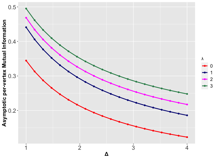
(a) Mutual information vs $\Delta$

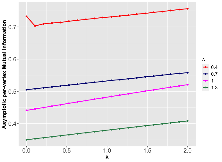
(b) Mutual information vs $\lambda$

Figure 1: Plot of asymptotic per vertex mutual information between $(\bm{\beta},\bm{\sigma})$ and $(\bm{y},\bm{G})$. For figure (a), we plot the mutual information (MI) as a function of $\Delta$. Note that as the noise strength $\Delta$ increases, the limiting MI decreases. The case $\lambda=0$ corresponsds to the setting with no graph side information. We see that the graph information increases the limiting MI in the model. In figure (b), we plot the limiting MI as a function of $\lambda$. We again see that as the signal strength $\lambda$ increases, the asymptotic MI increases in the model.

We observe in Figure 1(a) that if $\Delta$ is large, that is, we have significant noise in $\bm{y}$, the observed graph $\bm{G}$ adds significant information to our estimation procedure which increases with increasing $\lambda$. But in Figure 1(b), it is clear that the advantage in observing network information decreases with an increase in $\Delta$.

3.2 Comparison of Reconstruction Error between AMP-based estimator and estimator based on Graph Constrained Regression

3.2.1 Gaussian Design Matrix

In this subsection, we compare our AMP-based estimation of $\bm{\beta}$ with an estimator based on Laplacian penalization [44]. We set $n=p=3000$. For $1\leq i\leq p$, let $\sigma_{i}$ be independent samples from $\mathsf{Bern}(0.7)$. Given $\sigma_{i}=0$, set $\beta_{i}=0$ with probability $1$. If $\sigma_{i}=1$, generate $\beta_{i}$ from the uniform distribution on $\{\pm 1\}$. The graph $\bm{G}$ is generated according to (1.3). The entries of the feature matrix $\bm{\Phi}$ are generated i.i.d from $\mathsf{N}(0,p^{-0.5})$, and the observation vector $\bm{y}$ is generated according to (1.2). We fix $\lambda$ to be in the set $\{3,5\}$ and $b_{p}=0.7$. Using the relation (2.1), the parameter $a_{p}$ is set to be equal to

$$a_{p}=b_{p}+\sqrt{\frac{\lambda b_{p}(1-b_{p})}{p}}.$$

We vary $\Delta$ in an equispaced grid with $20$ points in $[0.2,4]$.

Next, we compute the estimates $\widehat{\bm{\beta}}_{\mathsf{Lap}}$ and $\widehat{\bm{\beta}}_{\mathsf{AMP}}$ where $\widehat{\bm{\beta}}_{\mathsf{Lap}}$ is the estimator computed using the method described in [44] and $\widehat{\bm{\beta}}_{\mathsf{AMP}}$ is computed by the AMP iterations described by (1.5) and (1.7). We run the AMP algorithm for 25 iterations to generate our estimates. For each combination of $(\lambda,\Delta)$ we repeat the experiment $20$ times independently and for each iteration we compute the empirical reconstruction errors

$$\mathcal{E}_{\mathsf{Lap}}=\frac{1}{p}\|\bm{\Phi}(\widehat{\bm{\beta}}_{\mathsf{Lap}}-\bm{\beta})\|^{2},$$

and

$$\mathcal{E}_{\mathsf{AMP}}=\frac{1}{p}\|\bm{\Phi}(\widehat{\bm{\beta}}_{\mathsf{AMP}}-\bm{\beta})\|^{2}.$$

We approximate the reconstruction errors by the sample average of the estimates across the independent replications. The plots of the estimated reconstruction errors are shown in Figure 2.

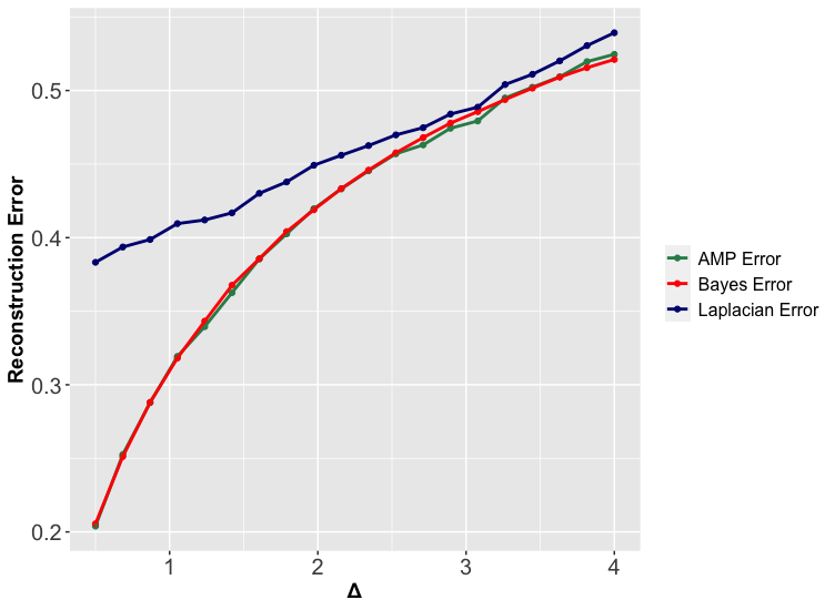
(a) $\lambda=3$

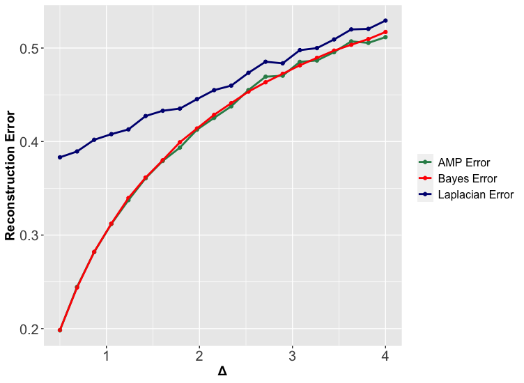
(b) $\lambda=5$

Figure 2: Plot of the average reconstruction error of $\widehat{\bm{\beta}}_{\mathsf{Lap}}$ and $\widehat{\bm{\beta}}_{\mathsf{AMP}}$ for Gaussian design matrix

We observe that the AMP-based estimator $\widehat{\bm{\beta}}_{\mathsf{AMP}}$ performs consistently better than $\widehat{\bm{\beta}}_{\mathsf{LP}}$ for both values of $\lambda$. In fact, the performance of $\widehat{\bm{\beta}}_{\mathsf{AMP}}$ in terms of the reconstruction error is approximately equal to the Bayes error in estimating $\bm{\beta}$ with the specified priors. The observed gaps are due to finite sample effects. The simulations demonstrate that if the prior is known, it is much more efficient to incorporate the prior information through AMP based algorithms.

3.2.2 Robustness to design distribution

Our theoretical results are derived under an iid gaussian assumption on the entries of the design matrix. AMP style algorithms are known to be quite robust to the design distribution [10, 22, 28, 69], and we expect the algorithms introduced in this paper to enjoy similar universality properties.

To this end, we provide initial numerical evidence to the universality properties of this algorithm. The work under the same setup reported in the previous subsection, but construct the design $\bm{\Phi}$ using iid centered and normalized $\mathsf{Ber}(0.3)$ entries. We plot the reconstruction error in Figure 3(b). We note that the main takeaways remain the same—the AMP algorithm still outperforms the Laplacian penalization based algorithm. We believe that using the ideas introduced in [28, 69], it should not be too difficult to establish the universality property for this class of AMP algorithms.

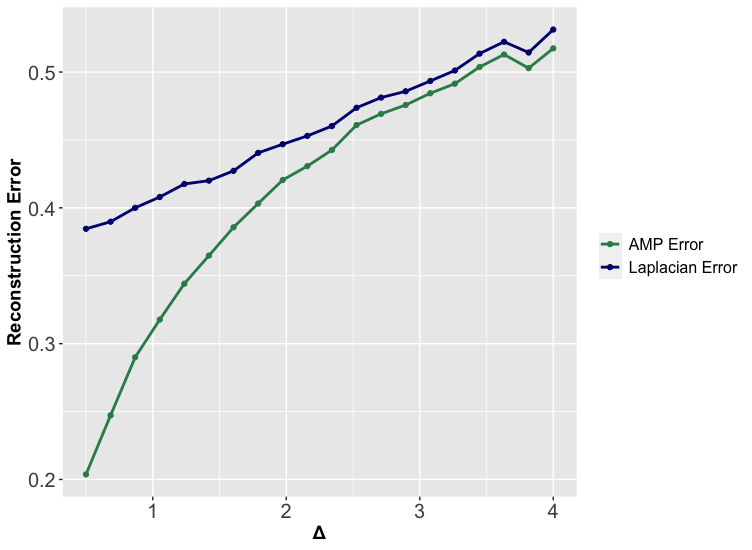
(a) $\lambda=3$

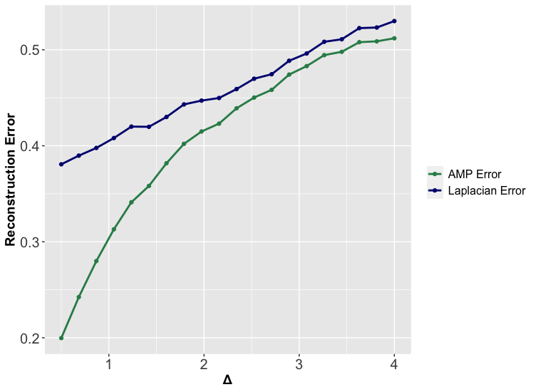
(b) $\lambda=5$

Figure 3: Plot of the average reconstruction error of $\widehat{\bm{\beta}}_{\mathsf{Lap}}$ and $\widehat{\bm{\beta}}_{\mathsf{AMP}}$ for Bernoulli Design Matrix

3.3 Variable discovery: AMP vs. Model-X Knockoff

In this section, we explore the variable discovery properties of the AMP based algorithm introduced in Section 1.1.3.

Knockoffs [4, 18] have emerged as the canonical choice for variable discovery in supervised learning problems. This methodology is attractive due to the finite sample guarantees on the FDR, along with high power in most practical settings.

In this section, we compare the performance of the AMP based algorithm to the statistical performance of the Model-X framework. Note that the Model-X framework ignores the graph information, and thus this is not a fair comparison in principle. Here, we invoke the Model-X methodology as the canonical algorithm for variable discovery in the absence of graph-side information—this helps us explore the practical gains obtained from the graph-side information.

3.3.1 Power comparison

In this section, we compare the performance of the variable discovery mechanism stated in Section 1.1.3 with Model-X knockoff in terms of the True Discovery Ratio given by

$$\mathrm{TDR}(\alpha,t;n):=\mathbb{E}\left[\frac{|\hat{S}(\alpha;t)|\cap|\{i:\sigma_{i}\neq 0\}|}{1\vee|\hat{S}(\alpha;t)|}\right].$$

Here $\hat{S}(\alpha;t)$ is as defined in Section 1.1.3. We take the generative model with the same $n,p$ and the prior distribution for $\bm{\beta}$ given $\bm{\sigma}$ as Section 3.2.1, but now we generate $\sigma_{i}$ for $i=1,\cdots,p$ independently from $\mathsf{Ber}(0.07)$ to induce sparsity in the model. We compare the performances of our methods versus Model-X knockoff for $\lambda=5,10$ and 5 equispaced $\Delta$ lying between $0.5$ and $4$. We tabulate the Monte Carlo estimates of the TDR over 20 independent runs of the experiment in Table 1. We observe that irrespective of the values of $\Delta$ and $\lambda$, our variable selection procedure performs uniformly better than Model-X knockoff that ignores the graph side information.

$\Delta$	$\lambda=5$		$\lambda=10$
	AMP	Knockoff	AMP	Knockoff
0.5	0.805	0.641	0.856	0.787
1.05	0.651	0.433	0.775	0.658
1.79	0.605	0.456	0.542	0.475
2.52	0.438	0.133	0.470	0.404
3.26	0.338	0.231	0.217	0.199
4.00	0.17	0.09	0.3	0.2

Table 1: Performance Comparison between the TDR of AMP-based variable selection and Model-X Knockoff-based variable selection

4 Discussion

In this paper, we formulated the problem of supervised learning with graph-side information in terms of a simple generative model and introduced an AMP-based algorithm to combine the information from the two sources. We also derived the asymptotic mutual information in this model and established that in many settings, this algorithm is, in fact, Bayes optimal. Finally, our numerical experiments establish the improvements obtained by this aggregation scheme.

In this section, we discuss some current limitations of these results, and opportunities to go beyond these barriers. In turn, this automatically suggests some natural directions for future inquiry.

• Generalization to account for more than 1 planted community—In this paper, we study a simple setting with one planted community. Of course, in the applications discussed in the introduction, it is probably more natural to assume the presence of multiple planted communities, with different connection probabilities for variables in distinct communities. We expect that the technical framework introduced in this paper can be extended to this setting in a straightforward manner, and present the 1 community case for ease of exposition.

• Incorporating correlation among the features—We assume independent gaussian features in our regression model. In many practical settings, it might be more realistic to have correlated features. For example, one could study a setting where the rows $\phi_{\mu}\in\mathbb{R}^{p}$ are i.i.d. samples from $N(0,\Sigma)$. It should be possible to design AMP-based algorithms for estimation and variable discovery even in this setting, using the ideas in [36, 48, 23]. However, it is particularly challenging to characterize the Bayes optimal performance in the correlated setting. Specifically, evaluation of the limiting mutual information will require new ideas. We believe this will be a very interesting direction for follow up investigations.

• The need for empirical Bayes approaches—The AMP algorithm introduced in this paper explicitly uses knowledge of the problem parameters $\rho$, $\Delta$, $a_{p}$, $b_{p}$ and the Markov kernel $P(\cdot|\cdot)$. In our discussions, we assume that these problem parameters are known. In practice, some or all of these parameters might be unknown. To make the algorithms practicable in this case, the unknown parameters need to be estimated from the given data. We note that the estimation of the graph connectivity parameters $a_{p}$, $b_{p}$ has been explored in the previous literature [54]. In a similar vein, the estimation of the noise variance $\Delta$ and the underlying sparsity $\rho$ have been explored in the statistical literature (see e.g. [40] and references therein). In this context, the estimation of the kernel $P(\cdot|\cdot)$ is expected to be the most challenging. One natural idea to estimate the conditional distribution would be to use empirical Bayesian methods [59]. We refer the interested reader to a recent application of this idea to the PCA problem in [71]. While this would be extremely interesting to explore, we feel that this is substantially beyond the scope of this paper, and we defer this to follow-up investigations. We note here that even if the Markov kernel $P(\cdot|\cdot)$ is unknown, the AMP algorithm can be implemented with any arbitrary kernel $Q(\cdot|\cdot)$, and the performance of the algorithm can be tracked using state evolution. Of course, if $P$ and $Q$ are quite different, the AMP performance is expected to be sub-optimal compared to the Bayes optimal performance.

• Statistical/Computational gaps in this problem—In Theorem 1.3, we noted that the AMP algorithm attains Bayes optimal performance if $(\mu^{*},\xi^{*})=(\bar{\mu},\bar{\xi})$. Of course, this equality could be violated for certain parameters $(a_{p},b_{p},\rho,\Delta,P)$. In this case, we conjecture the existence of a statistical-computational gap in this problem, and that the performance of the AMP algorithm represents the best statistical performance among computationally feasible algorithms. Statistical/Computational gaps have been conjectured in similar problems in the recent literature (see e.g. [15, 1, 41, 19, 24] and references therein for a very incomplete list), and there has been significant recent progress in favor of this conjecture by analyzing specific sub-classes of algorithms (e.g. based on convex penalized estimators [19], first-order methods [20], low degree algorithms [53, 62], query lower bounds [26] etc.). We believe that it should be possible to adapt the existing techniques to establish statistical/computational gaps in this problem. We refrain from exploring this direction in this paper to keep our discussion focused.

Acknowledgments:

SS thanks Jishnu Das for introducing him to the HotNet2 procedure, which motivated this work. SS gratefully acknowledges support from NSF (DMS CAREER 2239234), ONR (N00014-23-1-2489), AFOSR (FA9950-23-1-0429) and a Harvard FAS Dean’s competitive fund award. SN thanks Zongming Ma for many helpful discussions. We thank Lenka Zdeborová and Jean Barbier for pointing us to several relevant references, and helpful discussions.

Appendix A Proof of Theorem 1.2

We employ the adaptive interpolation approach of Barbier and Macris, 2019a [7] (see also [6, 9] and references therein) to characterize the mutual information in this setting.

We first connect the Regression plus Graph model to an equivalent Regression plus Gaussian Orthogonal Ensemble model. The model is described as follows. Given $\sigma_{1},\cdots,\sigma_{p}$ generated from $\mbox{Bernaulli}(\rho)$ distribution, we still observe the pair $(\bm{y},\bm{\Phi})$ generated by the linear model described by (1.2). But the random network $G$ is replaced by a Gaussian Model described by,

$$\widetilde{\bm{A}}=\sqrt{\frac{\lambda}{p}}\bm{\sigma}\bm{\sigma}^{\top}+\bm{Z},$$

where $Z_{ij}=Z_{ji}\sim N(0,1)$ if $i\neq j$ and $Z_{ii}\sim N(0,2)$. From the definition of mutual information, we get the following.

$$\lim\limits_{p\rightarrow\infty}\frac{1}{p}I(\bm{\beta}_{0},\bm{\sigma};\widetilde{\bm{A}},\bm{\Phi},\bm{y}) =\lim\limits_{p\rightarrow\infty}\frac{1}{p}\mathbb{E}_{(\bm{\beta}_{0},\bm{\sigma},\bm{\Phi},\bm{Z},\bm{\varepsilon})}\left[\log\frac{P(\widetilde{\bm{A}},\bm{y}\,|\,\bm{\beta}_{0},\bm{\sigma})}{P(\widetilde{\bm{A}},\bm{y})}\right]$$ (A.1)

$$=\mathbb{E}_{(\Sigma,B_{0})}[\log P(B_{0}\,|\,\Sigma)Q(\Sigma)]+\frac{\lambda}{4}(\mathbb{E}[\Sigma^{2}])^{2}-\lim\limits_{p\rightarrow\infty}\frac{1}{p}\mathbb{E}[\log\mathcal{Z}(\bm{\sigma},\bm{\beta}_{0})],$$ (A.2)

where,

$$\mathcal{Z}(\bm{\sigma},\bm{\beta}_{0})=\int\limits_{\bm{x},\bm{\beta}}\left\{\prod\limits_{i=1}^{p}dx_{i}\,d\beta_{i}\,Q(x_{i})P(\beta_{i}|x_{i})\right\}\exp\left(-\mathcal{H}_{n}(\bm{x},\bm{\beta};\bm{\sigma},\bm{\beta}_{0},\bm{\Phi},\bm{\varepsilon},\bm{Z})\right).$$

Here the Hamiltonian $\mathcal{H}_{n}$ is given by

$$\mathcal{H}_{n}(\bm{x},\bm{\beta};\bm{\sigma},\bm{\beta}_{0},\bm{\Phi},\bm{\varepsilon},\bm{Z}) =\lambda\sum\limits_{i\leq j=1}^{p}\left\{\frac{x^{2}_{i}x^{2}_{j}}{2p}-\frac{x_{i}x_{j}\sigma_{i}\sigma_{j}}{p}-\frac{x_{i}x_{j}Z_{ij}}{\sqrt{\lambda p}}\right\}$$ (A.3)

$$+\frac{1}{\Delta}\sum\limits_{\mu=1}^{n}\left\{\frac{1}{2}[\bm{\Phi}(\bm{\beta}-\bm{\beta}_{0})]^{2}_{\mu}-[\bm{\Phi}(\bm{\beta}-\bm{\beta}_{0})]_{\mu}\varepsilon_{\mu}\sqrt{\Delta}\right\}.$$ (A.4)

So, to understand the asymptotics of the per-vertex mutual information it is useful to study the asymptotics of the Bethe Free Energy of the model given by

$$f_{p}:=-\frac{1}{p}\mathbb{E}_{(\bm{\sigma},\bm{\beta}_{0},\bm{Z},\bm{\varepsilon},\bm{\Phi})}\mathbb{E}[\log\mathcal{Z}(\bm{\sigma},\bm{\beta}_{0})].$$

A.1 Asymptotics of the Free Energy

Interpolating Hamiltonian

We consider a sequence of interpolating Hamiltonians between the true Hamiltonian and the mean field Hamiltonian defined below. Consider the functions

$$h(\bm{x},\bm{\beta};\bm{\sigma},\bm{\beta}_{0},\bm{\Phi},\bm{\varepsilon},\theta^{2}_{1},\theta^{2}_{2}) =\frac{1}{\theta^{2}_{1}}\sum\limits_{\begin{subarray}{c}i\leq j\\ i,j=1\end{subarray}}^{p}\left\{\frac{x^{2}_{i}x^{2}_{j}}{2p}-\frac{x_{i}x_{j}\sigma_{i}\sigma_{j}}{p}-\theta_{1}\frac{x_{i}x_{j}Z_{ij}}{\sqrt{p}}\right\}$$ (A.5)

$$+\frac{1}{\theta^{2}_{2}}\sum\limits_{\mu=1}^{n}\left\{\frac{[\bm{\Phi}(\bm{\beta}-\bm{\beta}_{0})]^{2}_{\mu}}{2}-\theta_{2}[\bm{\Phi}(\bm{\beta}-\bm{\beta}_{0})]_{\mu}\varepsilon_{\mu}\right\},$$ (A.6)

and

$$h_{mf}(\bm{x},\bm{\beta};\bm{\sigma},\bm{\beta}_{0},\bm{\Phi},\bm{\varepsilon},\theta^{2}_{1},\theta^{2}_{2}) =\frac{1}{\theta^{2}_{1}}\sum\limits_{i=1}^{p}\left\{\frac{x^{2}_{i}}{2}-x_{i}\sigma_{i}-\theta_{1}x_{i}\widebar{Z_{i}}\right\}$$ (A.7)

$$+\frac{1}{\theta^{2}_{2}}\sum\limits_{j=1}^{p}\left\{\frac{(\beta_{j}-\beta_{0j})^{2}}{2}-\theta_{2}(\beta_{j}-\beta_{0j})\widebar{\varepsilon}_{j}\right\}.$$ (A.8)

Now consider interpolating parameters $\{E_{k}\}_{k=1}^{K}$; $\Sigma_{k}:=\Sigma(E_{k};\Delta)$ and $\{q_{k}\}_{k=1}^{K}$. Then, for $\bm{\eta}=(\eta_{1},\eta_{2})$, where $\eta_{1},\eta_{2}>0$, consider the $(k,t)-$Interpolating Hamiltonian given by,

$$\mathcal{H}_{k,t;\bm{\eta}}\left(\bm{x},\bm{\beta};\bm{\sigma},\bm{\beta}_{0},\Theta\right) :=\sum\limits_{\ell>k+1}h(\bm{x},\bm{\beta};\bm{\sigma},\bm{\beta}_{0},\bm{\Phi},\bm{\varepsilon}_{\ell},\bm{Z}_{\ell},K/\lambda,K\Delta)$$ (A.9)

$$\hskip 14.45377pt+\sum\limits_{\ell=1}^{k-1}h_{mf}(\bm{x},\bm{\beta};\bm{\sigma},\bm{\beta}_{0},\bm{\Phi},\widebar{\bm{\varepsilon}}_{\ell},\widebar{\bm{Z}}_{\ell},K/\lambda q_{\ell},K\Sigma^{2}_{\ell})$$ (A.10)

$$\hskip 14.45377pt+h(\bm{x},\bm{\beta};\bm{\sigma},\bm{\beta}_{0},\bm{\Phi},\bm{\varepsilon}_{k},\bm{Z}_{k},K/\lambda(1-t),K/\gamma_{k}(t))$$ (A.11)

$$\hskip 14.45377pt+h_{mf}(\bm{x},\bm{\beta};\bm{\sigma},\bm{\beta}_{0},\bm{\Phi},\widebar{\bm{\varepsilon}}_{k},\widebar{\bm{Z}}_{k},K/\lambda tq_{k},K/\lambda_{k}(t))$$ (A.12)

$$\hskip 14.45377pt+\eta_{1}\sum\limits_{i=1}^{p}\left\{\frac{x^{2}_{i}}{2}-\sigma_{i}x_{i}-\frac{x_{i}\widehat{Z}_{i}}{\sqrt{\eta_{1}}}\right\}+\eta_{2}\sum\limits_{i=1}^{p}\left\{\frac{(\beta_{i}-\beta_{0i})^{2}}{2}-\frac{(\beta_{i}-\beta_{0i})\widehat{\widehat{Z}}_{i}}{\sqrt{\eta_{2}}}\right\},$$ (A.13)

where $\Theta:=(\bm{\Phi},\{\bm{\varepsilon}_{\ell}\}_{\ell=1}^{K},\{\bm{Z}_{\ell}\}_{\ell=1}^{K},\{\widebar{\bm{\varepsilon}}_{\ell}\}_{\ell=1}^{K},\{\widebar{\bm{Z}}_{\ell}\}_{\ell=1}^{K},\{\widehat{Z}_{\ell}\}_{\ell=1}^{K},\{\widehat{\widehat{Z}}_{\ell}\}_{\ell=1}^{K},\{q_{k}\}_{k=1}^{K},\{E_{k}\}_{k=1}^{K})$ and $\{\bm{\varepsilon}_{\ell}\}_{\ell=1}^{K}\overset{i.i.d}{\sim}N_{p}(\bm{0},\bm{I}_{p})$, $\{\widebar{\bm{\varepsilon}}_{\ell}\}_{\ell=1}^{K}\overset{i.i.d}{\sim}N_{n}(\bm{0},\bm{I}_{n})$, $\{\bm{Z}_{\ell}\}_{\ell=1}^{K}\overset{i.i.d}{\sim}\sqrt{p}\,GOE(p)$, $\{\widebar{\bm{Z}}_{\ell}\}_{\ell=1}^{K}\overset{i.i.d}{\sim}N_{p}(\bm{0},\bm{I}_{p})$, $\{\widehat{Z}_{\ell}\}_{\ell=1}^{K}\overset{i.i.d}{\sim}N(0,1)$ and $\{\widehat{\widehat{Z}}_{\ell}\}_{\ell=1}^{K}\overset{i.i.d}{\sim}N(0,1)$. Assume that $\gamma_{k},\lambda_{k}:[0,1]\rightarrow\mathbb{R}$ satisfying

$$\gamma_{k}(0)=\Delta^{-1};\quad\lambda_{k}(0)=0;\quad\gamma_{k}(1)=0,\quad\mbox{and}\quad\lambda_{k}(1)=\Sigma^{-2}_{k}.$$

The parameters $\gamma_{k}(t)$ and $\lambda_{k}(t)$ are implicitly defined by the following equations.

$$\frac{\kappa}{\gamma^{-1}_{k}(t)+E_{k}}+\lambda_{k}(t)=\Sigma^{-2}_{k}\quad\mbox{and thus,}\quad\frac{d\lambda_{k}(t)}{dt}=-\frac{d\gamma_{k}(t)}{dt}\frac{\kappa}{(1+\gamma_{k}(t)E_{k})^{2}}.$$ (A.14)

Finally, let us define the interpolating free energy as follows.

$$f_{k,t;\bm{\eta}}=-\frac{1}{p}\mathbb{E}_{\Theta}\left[\log\int\left\{\prod\limits_{i=1}^{p}P(\beta_{i}|x_{i})Q(x_{i})d\beta_{i}dx_{i}\right\}\exp\left(-\mathcal{H}_{k,t;\bm{\eta}}(\bm{x},\bm{\beta};\Theta)\right)\right].$$ (A.15)

Boundary Cases.

Consider the following boundary cases.

$$\mathcal{H}_{1,0,0}(\bm{x},\bm{\beta};\Theta) =\sum\limits_{\ell=1}^{K}h(\bm{x},\bm{\beta};\bm{\sigma},\bm{\beta}_{0},\bm{\Phi},\bm{\varepsilon}_{\ell},\bm{Z}_{\ell},k/\lambda,k\Delta)$$ (A.16)

$$=\frac{\lambda}{K}\sum\limits_{\ell=1}^{K}\left\{\sum\limits_{\begin{subarray}{c}i\leq j\\ i,j=1\end{subarray}}^{p}\left[\frac{x^{2}_{i}x^{2}_{j}}{2p}-\frac{\sigma_{i}\sigma_{j}x_{i}x_{j}}{p}\right]\right\}-\sum\limits_{\begin{subarray}{c}i\leq j\\ i,j=1\end{subarray}}^{p}x_{i}x_{j}\sqrt{\frac{\lambda}{K}}\frac{1}{\sqrt{p}}\sum\limits_{\ell=1}^{K}Z^{(\ell)}_{ij}$$ (A.17)

$$\hskip 21.68121pt+\frac{1}{\Delta}\sum\limits_{\mu=1}^{n}\frac{1}{2}[\bm{\Phi}(\bm{\beta}-\bm{\beta}_{0})]^{2}_{\mu}-\frac{1}{\Delta}\sum\limits_{\mu=1}^{n}[\bm{\Phi}(\bm{\beta}-\bm{\beta}_{0})]_{\mu}\left(\frac{\sqrt{\Delta}}{\sqrt{K}}\sum\limits_{\ell=1}^{K}\varepsilon^{\ell}_{\mu}\right)$$ (A.18)

$$\overset{d}{=}\lambda\left\{\sum\limits_{\begin{subarray}{c}i\leq j\\ i,j=1\end{subarray}}^{p}\left[\frac{x^{2}_{i}x^{2}_{j}}{2p}-\frac{\sigma_{i}\sigma_{j}x_{i}x_{j}}{p}\right]\right\}-\sqrt{\frac{\lambda}{p}}\sum\limits_{\begin{subarray}{c}i\leq j\\ i,j=1\end{subarray}^{p}}x_{i}x_{j}Z_{ij}\quad\quad\mbox{[where $\bm{Z}\sim\sqrt{p}\;GOE(p)$]}$$ (A.19)

$$\hskip 21.68121pt+\frac{1}{\Delta}\sum\limits_{\mu=1}^{n}\frac{1}{2}[\bm{\Phi}(\bm{\beta}-\bm{\beta}_{0})]^{2}_{\mu}-\frac{1}{\Delta}\sum\limits_{\mu=1}^{n}[\bm{\Phi}(\bm{\beta}-\bm{\beta}_{0})]_{\mu}\sqrt{\Delta}\varepsilon_{\mu}\quad\quad\mbox{[where $\varepsilon_{\mu}\sim N(0,1)$]}.$$ (A.20)

Therefore, we have $f_{1,0,0}=f_{p}$. Next, let us observe that

$$\mathcal{H}_{K,1;0}(\bm{x},\bm{\beta};\Theta) =\sum_{\ell=1}^{K}h_{mf}(\bm{x},\bm{\beta};\bm{\sigma},\bm{\beta}_{0},\bm{\Phi},\widebar{\bm{\varepsilon}}_{k},\widebar{\bm{Z}}_{k},k/\lambda q_{k},k/\Sigma^{2}_{\ell})$$ (A.21)

$$=\lambda\widebar{q}_{K}\left\{\sum\limits_{i=1}^{p}\left[\frac{x^{2}_{i}}{2}-\sigma_{i}x_{i}-\sqrt{\frac{1}{\lambda\widebar{q}_{K}}}x_{i}\sum\limits_{\ell=1}^{K}\widebar{Z}^{\ell}_{i}\sqrt{\frac{q_{\ell}}{\widebar{q}_{K}}}\right]\right\}$$ (A.22)

$$\quad+\frac{1}{\Sigma^{2}_{K}}\left\{\sum\limits_{i=1}^{p}\left[\frac{(\beta_{i}-\beta_{0i})^{2}}{2}-\Sigma_{K}(\beta_{i}-\beta_{0i})\sum\limits_{\ell=1}^{K}\widebar{\varepsilon}^{(\ell)}_{i}\frac{\Sigma_{K}}{\Sigma_{\ell}}\frac{1}{\sqrt{K}}\right]\right\}$$ (A.23)

$$=h_{mf}(\bm{x},\bm{\beta};\bm{\sigma},\bm{\beta}_{0},\bm{\Phi},\bm{\varepsilon},(\lambda\bar{q}_{K})^{-1},\Sigma^{2}_{K}),$$ (A.24)

where

$$\Sigma^{-2}_{K}=\frac{1}{K}\sum_{\ell=1}^{K}\Sigma^{-2}_{\ell};\quad\quad\mbox{and}\quad\quad\widebar{q}_{K}=\frac{1}{K}\sum\limits_{\ell=1}^{K}q_{\ell}.$$ (A.25)

Replica Symmetric Potential

Next, we define the following.

$$f_{den}(\widetilde{\sigma}^{2}_{1},\widetilde{\sigma}^{2}_{2}) :=-\mathbb{E}_{\Theta}\Bigg{[}\log\int P(\beta|x)Q(x)\exp\Bigg{(}-\frac{1}{\widetilde{\sigma}^{2}_{1}}\left(\frac{x^{2}}{2}-\sigma x-\widetilde{\sigma}_{1}x\widebar{Z}\right)$$ (A.26)

$$\hskip 72.26999pt-\frac{1}{\widetilde{\sigma}^{2}_{2}}\left(\frac{(\beta-\beta_{0})^{2}}{2}-\widetilde{\sigma}_{2}(\beta-\beta_{0})\widebar{\varepsilon}\right)\Bigg{)}\Bigg{]},$$ (A.27)

where $\widebar{Z},\widebar{\varepsilon}\sim N(0,1)$. Therefore

$$f_{K,1;0}=f_{den}(1/\lambda\widebar{q}_{K},\Sigma^{2}_{K}).$$

We shall find $\lim_{p\rightarrow\infty}f_{p}$ in terms of $\widebar{q}_{K},\Sigma^{2}_{K}$ and $f_{den}$. Consider the following function.

$$f_{RS}(\lambda,q;E,\Delta):=\frac{\lambda q^{2}}{4}+\psi(E;\Delta)+f_{den}\left(\frac{1}{\lambda q},\Sigma^{2}(E,\Delta)\right),$$

where,

$$\Sigma(E,\Delta)^{-2}=\frac{\kappa}{\Delta+E};\quad\quad\psi(E,\Delta)=\frac{\kappa}{2}\left[\log\left(1+\frac{E}{\Delta}\right)-\frac{E}{E+\Delta}\right].$$

The random variables in the collection $\Theta$ will be called the quenched random variables and the expectation with respect to them will be denoted by $\mathbb{E}_{\Theta}$. The random variables $\{\bm{x},\bm{\beta}\}$ are called annealed random variables, and expectation with respect to them will be denoted by Gibb’s Bracket $\langle\cdot\rangle_{\mathcal{H}}$. The entire expression of the Hamiltonian $\mathcal{H}_{k,t;\eta}$ may be omitted from time to time and must be understood from the context. Let us define

$$P_{k,t;\bm{\eta}}(\bm{x},\bm{\beta}|\theta):=\frac{\prod_{i=1}^{p}P(x_{i})P(\beta_{i}|x_{i})\exp(-\mathcal{H}_{k,t;\eta}(\bm{x},\bm{\beta};\theta))}{\int\{\prod_{i=1}^{p}P(x_{i})P(\beta_{i}|x_{i})dx_{i}d\beta_{i}\}\exp(-\mathcal{H}_{k,t;\eta}(\bm{x},\bm{\beta};\theta)},$$

and

$$\langle A(\bm{X},\bm{\beta})\rangle_{\mathcal{H}_{k,t;\bm{\eta}}}:=\int A(\bm{x},\bm{\beta})P_{k,t;\bm{\eta}}(\bm{x},\bm{\beta}|\theta)d\bm{x}d\bm{\beta}.$$

Computation of $\frac{df_{k,t;\bm{\eta}}}{dt}$

Let us observe the following calculation.

$$\frac{df_{k,t;\bm{\eta}}}{dt}=\frac{1}{p}\mathbb{E}_{\Theta}\left[\left\langle\frac{d\mathcal{H}_{k,t;\bm{\eta}}}{dt}\right\rangle_{\mathcal{H}_{k,t;\bm{\eta}}}\right].$$

Further, we have the following identity.

$$\frac{d\mathcal{H}_{k,t;\bm{\eta}}}{dt} =\frac{d}{dt}h_{mf}(\bm{x},\bm{\beta};\bm{\sigma},\bm{\beta}_{0},\bm{\Phi},\widebar{\bm{\varepsilon}}_{k},\widebar{\bm{Z}}_{k},K/\lambda tq_{k},K/\lambda_{k}(t))$$ (A.28)

$$\quad\quad+\frac{d}{dt}h(\bm{x},\bm{\beta};\bm{x},\bm{\beta},\bm{\Phi},\bm{\varepsilon}_{k},\bm{Z}_{k},K/(1-t)\lambda,K/\gamma_{k}(t))$$ (A.29)

$$=\frac{\lambda q_{k}}{K}\sum\limits_{i=1}^{p}\left(\frac{x^{2}}{2}-x_{i}\sigma_{i}-\frac{x_{i}\widebar{Z}^{(k)}_{i}}{2}\sqrt{\frac{K}{tq_{k}\lambda}}\right)$$ (A.30)

$$\quad+\frac{d\lambda_{k}(t)}{dt}\frac{1}{2K}\sum\limits_{j=1}^{p}\left((\beta_{j}-\beta_{0j})^{2}-\sqrt{\frac{K}{\lambda_{k}(t)}}(\beta_{j}-\beta_{0j})\widebar{\varepsilon}^{(k)}_{j}\right)$$ (A.31)

$$-\frac{\lambda}{K}\sum\limits_{\begin{subarray}{c}i\leq j\\ i,j=1\end{subarray}}^{p}\left\{\frac{x^{2}_{i}x^{2}_{j}}{2p}-\frac{x_{i}x_{j}\sigma_{i}\sigma_{j}}{p}-\frac{x_{i}x_{j}Z^{(k)}_{ij}}{2\sqrt{p}}\sqrt{\frac{K}{(1-t)\lambda}}\right\}$$ (A.32)

$$\quad+\frac{d\gamma_{k}(t)}{dt}\frac{1}{2K}\sum\limits_{\mu=1}^{n}\left\{[\bm{\Phi}(\bm{\beta}-\bm{\beta}_{0})]^{2}_{\mu}-\sqrt{\frac{K}{\gamma_{k}(t)}}[\bm{\Phi}(\bm{\beta}-\bm{\beta}_{0})]_{\mu}\varepsilon^{(k)}_{\mu}\right\}.$$ (A.33)

We consider the Nishimori Identity given below.

$$\mathbb{E}\left[\langle g(\bm{x},\bm{\beta},\bm{\sigma},\bm{\beta}_{0})\rangle_{\mathcal{H}_{k,t;\bm{\eta}}}\right]=\mathbb{E}\left[\langle g(\bm{x},\bm{\beta},\bm{x}^{\prime},\bm{\beta}^{\prime})\rangle_{\mathcal{H}_{k,t;\bm{\eta}}}\right],$$ (A.34)

where $(\bm{x},\bm{\beta})$ and $(\bm{x}^{\prime},\bm{\beta}^{\prime})$ are drawn i.i.d from $P_{k,t;\bm{\eta}}(\bm{x},\bm{\beta}|\Theta)$. From (A.28) and Gaussian Integration by parts we get the following.

$$\frac{d\,f_{k,t;\bm{\eta}}}{dt} =\frac{\lambda}{pK}\mathbb{E}\left[\left\langle q_{k}\sum\limits_{i=1}^{p}\left(\frac{x_{i}x^{\prime}_{i}}{2}-x_{i}\sigma_{i}\right)-\sum\limits_{i\leq j=1}^{p}\left(\frac{x_{i}x_{j}x^{\prime}_{i}x^{\prime}_{j}}{2p}-\frac{x_{i}x_{j}\sigma_{i}\sigma_{j}}{p}\right)\right\rangle\right]$$ (A.35)

$$\quad+\frac{d\gamma_{k}(t)}{dt}\frac{1}{2pK}\sum\limits_{\mu=1}^{n}\mathbb{E}\left[\left\langle[\bm{\Phi}(\bm{\beta}-\bm{\beta}_{0})]_{\mu}\right\rangle^{2}\right]+\frac{d\lambda_{k}(t)}{dt}\frac{1}{2pK}\sum\limits_{i=1}^{p}\mathbb{E}\left[\left\langle\bm{\beta}-\bm{\beta}_{0}\right\rangle^{2}\right].$$ (A.36)

Let us define the following equation.

$$\widebar{\mathsf{y}}_{\mathrm{mmse}}:=\frac{1}{n}\mathbb{E}[\|\bm{\Phi}(\langle\bm{\beta}\rangle-\bm{\beta}_{0})\|^{2}_{2}]\quad\mbox{and}\quad\mathsf{mmse}=\frac{1}{p}\mathbb{E}[\|\langle\bm{\beta}\rangle-\bm{\beta}_{0}\|^{2}_{2}].$$ (A.37)

Therefore

$$\frac{df_{k,t;\bm{\eta}}}{dt} =\frac{\lambda}{pK}\mathbb{E}\left[\left\langle q_{k}\sum\limits_{i=1}^{p}\left(\frac{x_{i}x^{\prime}_{i}}{2}-x_{i}\sigma_{i}\right)-\sum\limits_{\begin{subarray}{c}i\leq j\\ i,j=1\end{subarray}}^{p}\left(\frac{x_{i}x_{j}x^{\prime}_{i}x^{\prime}_{j}}{2p}-\frac{x_{i}x_{j}\sigma_{i}\sigma_{j}}{p}\right)\right\rangle\right]$$ (A.38)

$$\quad+\frac{d\gamma_{k}(t)}{dt}\frac{\kappa}{2K}\left[\widebar{\mathsf{y}}_{\mathrm{mmse}}-\frac{1}{(1+\gamma_{k}(t)E_{k})^{2}}\mathsf{mmse}\right],$$ (A.39)

where the last equality follows from (A.14). Now using (A.34); we get

$$\frac{df_{k,t;\bm{\eta}}}{dt} =\mathbb{E}\left[\left\langle-\frac{\lambda}{pK}\frac{q_{k}}{2}\sum\limits_{i=1}^{p}\sigma_{i}x_{i}+\frac{\lambda}{2Kp^{2}}\sum_{\begin{subarray}{c}i\leq j\\ i,j=1\end{subarray}}^{p}x_{i}x_{j}\sigma_{i}\sigma_{j}\right\rangle\right]+\frac{\kappa}{2K}\left[\widebar{\mathsf{y}}_{\mathrm{mmse}}-\frac{1}{(1+\gamma_{k}(t)E_{k})^{2}}\mathsf{mmse}\right].$$ (A.40)

Now let us observe that

$$\sum\limits_{\begin{subarray}{c}i\leq j\\ i,j=1\end{subarray}}^{p}x_{i}x_{j}\sigma_{i}\sigma_{j}=\frac{1}{2}\sum\limits_{\begin{subarray}{c}i,j=1\\ i<j\end{subarray}}^{p}x_{i}x_{j}\sigma_{i}\sigma_{j}+\frac{1}{2}\sum\limits_{i=1}^{p}x^{2}_{i}\sigma^{2}_{i}.$$

Hence, using the Cauchy Schwartz Inequality and the Nishimori Identity, we get

$$\mathbb{E}\left[\left\langle\frac{1}{n}\sum\limits_{i=1}^{n}x^{2}_{i}\sigma^{2}_{i}\right\rangle\right]\leq\left(\mathbb{E}\left[\left\langle\frac{1}{n}\sum\limits_{i=1}^{p}x^{4}_{i}\right\rangle\right]\right)^{1/2}\left(\mathbb{E}\left[\left\langle\frac{1}{n}\sum\limits_{i=1}^{p}\sigma^{4}_{i}\right\rangle\right]\right)^{1/2}=\mathbb{E}[\sigma^{4}].$$

Therefore, we have

$$\frac{d\,f_{k,t;\bm{\eta}}}{dt}=\mathbb{E}\left[\left\langle\frac{\lambda}{4K}s^{2}_{\bm{x},\bm{\sigma}}-\frac{\lambda q_{k}}{K}s_{\bm{x},\bm{\sigma}}\right\rangle\right]+\frac{\kappa}{2K}\left[\widebar{\mathsf{y}}_{\mathrm{mmse}}-\frac{1}{(1+\gamma_{k}(t)E_{k})^{2}}\mathsf{mmse}\right]+O\left(\frac{1}{nK}\right),$$ (A.41)

where $s_{\bm{x},\bm{\sigma}}=(1/p)\sum\limits_{i=1}^{p}\sigma_{i}x_{i}$ is the empirical overlap.

Free Energy Change along the Interpolation Path:

Let us consider the following equation.

$$f_{1,0,\bm{\eta}} =f_{K,1;\bm{\eta}}+\sum\limits_{k=1}^{K}(f_{k,0;\bm{\eta}}-f_{k,1;\bm{\eta}})$$ (A.42)

$$=f_{K,1;\bm{\eta}}-\sum\limits_{k=1}^{K}\int\limits_{0}^{1}\frac{df_{k,t;\bm{\eta}}}{dt}\,dt.$$ (A.43)

We consider the following lemma characterizing the concentration of the empirical overlap $s_{\bm{x},\bm{\sigma}}$ around its mean.

Lemma A.1.

For $K_{p}\rightarrow\infty$, $0<a_{p}<b_{p}<1$ and any choice of parameters $\{q_{k}\}_{k=1}^{K_{p}}$, functions of $\eta_{1}$, i.e., $q_{k}:\eta_{1}\rightarrow\mathbb{R}_{+}$ which are differentiable, bounded and non-decreasing with respect to $\eta_{1}$ when $\eta_{2}$ is held constant; we have $C>0$ and $0<\alpha<1/4$ such that,

$$\int\limits_{a^{(1)}_{p}}^{b^{(1)}_{p}}d\eta_{1}\left(\frac{1}{K_{p}}\sum\limits_{k=1}^{K_{p}}\int\limits_{0}^{1}dt\,\mathbb{E}\left[\left\langle(s_{\bm{x},\bm{\sigma}}-\mathbb{E}[\langle s_{\bm{x},\bm{\sigma}}\rangle])^{2}\right\rangle\right]\right)\leq\frac{C}{(a^{(1)}_{p})^{2}p^{\alpha}},$$

where the Hamiltonian is computed with respect to the parameters $\{q_{k}\}_{k=1}^{K_{p}}$.

Further, also consider the following lemma characterizing the concentration of $\mathsf{y_{mmse}}$.

Lemma A.2.

Again, let $K_{p}\rightarrow\infty$ and $0<a^{(2)}_{p}<b^{(2)}_{p}<1$; sequence of parameters $\{E_{k}\}_{k=1}^{K_{p}}$, where as a function of $\eta_{2}$, $E_{k}(\eta_{2})$ is bounded, differentiable and non0increasing in $\eta_{2}$ when $\eta_{1}$ is constant. Then we have,

$$\int\limits_{a^{(2)}_{p}}^{b^{(2)}_{p}}d\eta_{2}\left(\frac{1}{K_{p}}\sum\limits_{k=1}^{K_{p}}\int\limits_{0}^{1}dt\frac{d\gamma_{k}(t)}{dt}\left\{\mathsf{y_{mmse}}-\frac{\mathsf{mmse}}{1+\gamma_{k}(t)\mathsf{mmse}}\right\}\right)=O\left(\frac{1}{(a^{(2)}_{p})^{2}p^{\alpha}}\right).$$

For a sequence of parameters $\{q_{k}\}_{k=1}^{K}$, let us define,

$$V_{K}(\{q_{k}\}_{k=1}^{K})=\frac{1}{K}\sum\limits_{k=1}^{K}q^{2}_{k}-\left(\frac{1}{K}\sum\limits_{k=1}^{K}q_{k}\right)^{2}.$$

Now by (A.41), we get

$$\int\limits_{a^{(1)}_{p}}^{b^{(1)}_{p}}\int\limits_{a^{(2)}_{p}}^{b^{(2)}_{p}}d\eta_{1}d\eta_{2}f_{1,0;\bm{\eta}} =\int\limits_{a^{(1)}_{p}}^{b^{(1)}_{p}}\int\limits_{a^{(2)}_{p}}^{b^{(2)}_{p}}d\eta_{1}d\eta_{2}\Bigg{\{}(f_{K_{p},1;\bm{\eta}}-f_{K_{p},1;\bm{\eta}})+\frac{\lambda}{4}V_{K_{p}}(\{q_{k}\}_{k=1}^{K_{p}})\Bigg{\}}$$ (A.44)

$$\quad\quad-\frac{\lambda}{4}\int\limits_{a^{(1)}_{p}}^{b^{(1)}_{p}}\int\limits_{a^{(2)}_{p}}^{b^{(2)}_{p}}d\eta_{1}d\eta_{2}\left[\frac{1}{K_{p}}\sum\limits_{k=1}^{K_{p}}\int\limits_{0}^{1}\mathbb{E}\left[\langle(s_{\bm{x},\bm{\sigma}}-q_{k})^{2}\rangle\right]dt\right]$$ (A.45)

$$\quad-\frac{\kappa}{2}\int\limits_{a^{(1)}_{p}}^{b^{(1)}_{p}}\int\limits_{a^{(2)}_{p}}^{b^{(2)}_{p}}d\eta_{1}d\eta_{2}\frac{1}{K_{p}}\sum\limits_{k=1}^{K_{p}}\int\limits_{0}^{1}dt\,\frac{d\gamma_{k}(t)}{dt}\Bigg{[}\frac{\mathsf{mmse}}{1+\gamma_{k}(t)\mathsf{mmse}}-$$ (A.46)

$$\quad\quad\quad\frac{\mathsf{mmse}}{(1+\gamma_{k}(t)\mathsf{mmse})^{2}}+\frac{E_{k}}{(1+\gamma_{k}(t)\mathsf{mmse})^{2}}-\frac{E_{k}}{(1+\gamma_{k}(t)\mathsf{mmse})}\Bigg{]}$$ (A.47)

$$\quad+\int\limits_{a^{(1)}_{p}}^{b^{(1)}_{p}}\int\limits_{a^{(2)}_{p}}^{b^{(2)}_{p}}d\eta_{1}d\eta_{2}\widetilde{f}_{RS}\left(\{q_{k}\}_{k=1}^{K_{p}},\{E_{k}\}_{k=1}^{K_{p}},\Delta,\lambda\right)+O\left(\frac{1}{(a^{(1)}_{p}\wedge a^{(2)}_{p})^{2}p^{\alpha}}\right),$$ (A.48)

where

$$\widetilde{f}_{RS}\left(\{q_{k}\}_{k=1}^{K_{p}},\{E_{k}\}_{k=1}^{K_{p}},\Delta,\lambda\right)=\frac{\lambda}{4}\left(\frac{1}{K_{p}}\sum\limits_{k=1}^{K_{p}}q_{k}\right)^{2}+\frac{1}{K_{p}}\sum\limits_{k=1}^{K_{p}}\psi(\Delta;E_{k})+f_{den}\left(\frac{1}{\lambda\widebar{q}_{K_{p}}},\Sigma^{-2}_{K_{p}}\right),$$ (A.49)

and $\widebar{q}_{K_{p}},\Sigma^{2}_{K_{p}}$ are defined in (A.25). This follows as

$$\psi(E_{k};\Delta)=\frac{\kappa}{2}\int\limits_{0}^{1}dt\,\frac{d\gamma_{k}(t)}{dt}\left(\frac{E_{k}}{(1+\gamma_{k}(t)E_{k})^{2}}-\frac{E_{k}}{1+\gamma_{k}(t)E_{k}}\right).$$

Now by using (A.44) and Lemmas A.2 and A.1, we get the following equation.

$$\int\limits_{a^{(1)}_{p}}^{b^{(1)}_{p}}\int\limits_{a^{(2)}_{p}}^{b^{(2)}_{p}}d\eta_{1}d\eta_{2}f_{1,0;\bm{\eta}} =\int\limits_{a^{(1)}_{p}}^{b^{(1)}_{p}}\int\limits_{a^{(2)}_{p}}^{b^{(2)}_{p}}d\eta_{1}d\eta_{2}\Bigg{\{}(f_{K_{p},1;\bm{\eta}}-f_{K_{p},1;\bm{\eta}})+\frac{\lambda}{4}V_{K_{p}}(\{q_{k}\}_{k=1}^{K_{p}})\Bigg{\}}$$ (A.50)

$$\quad\quad-\frac{\lambda}{4}\int\limits_{a^{(1)}_{p}}^{b^{(1)}_{p}}\int\limits_{a^{(2)}_{p}}^{b^{(2)}_{p}}d\eta_{1}d\eta_{2}\left[\frac{1}{K_{p}}\sum\limits_{k=1}^{K_{p}}\int\limits_{0}^{1}\mathbb{E}\left\{\mathbb{E}[\langle s_{\bm{x},\bm{\sigma}}\rangle_{k,t;\bm{\eta}}]-q_{k}\right\}^{2}dt\right]$$ (A.51)

$$\quad-\frac{\kappa}{2}\int\limits_{a^{(1)}_{p}}^{b^{(1)}_{p}}\int\limits_{a^{(2)}_{p}}^{b^{(2)}_{p}}d\eta_{1}d\eta_{2}\frac{1}{K_{p}}\sum\limits_{k=1}^{K_{p}}\int\limits_{0}^{1}dt\,\frac{d\gamma_{k}(t)}{dt}\frac{\gamma_{k}(t)(E_{k}-\mathsf{mmse}_{k,t;\bm{\eta}})^{2}}{(1+\gamma_{k}(t)E_{k})^{2}(1+\gamma_{k}(t)\mathsf{mmse}_{k,t;\bm{\eta}})}$$ (A.52)

$$\quad+\int\limits_{a^{(1)}_{p}}^{b^{(1)}_{p}}\int\limits_{a^{(2)}_{p}}^{b^{(2)}_{p}}d\eta_{1}d\eta_{2}\widetilde{f}_{RS}\left(\{q_{k}\}_{k=1}^{K_{p}},\{E_{k}\}_{k=1}^{K_{p}},\Delta,\lambda\right)+O\left(\frac{1}{(a^{(1)}_{p}\wedge a^{(2)}_{p})^{2}p^{\alpha}}\right),$$ (A.53)

Upper Bound to the limit of the Free Energy

To get the upper bound to the asymptotic limit of the free energy let us consider the following lemma.

Lemma A.3.

For $\bm{\eta}=(\eta_{1},\eta_{2})$ and $f_{k,t;\bm{\eta}}$ defined in (A.15), we have constants $C_{1},C_{2}>0$,

$$\left|f_{1,0;\bm{\eta}}-f_{1,0;\bm{0}}\right|\leq C_{1}\|\bm{\eta}\|\quad\mbox{and}\quad\left|f_{K,1;\bm{\eta}}-f_{K,1;\bm{0}}\right|\leq C_{2}\|\bm{\eta}\|.$$

Let us choose the interpolation parameters as $(q_{k},E_{k}):=\operatorname*{arg\,min}\limits_{(q,E)\geq 0}f_{RS}(\lambda,q;E,\Delta)$. Then using (A.49), we get the following.

$$\widetilde{f}_{RS}\left(\{q_{k}\}_{k=1}^{K_{p}},\{E_{k}\}_{k=1}^{K_{p}},\Delta,\lambda\right)=\min\limits_{(q,E)\geq 0}f_{RS}(\lambda,q;E,\Delta).$$

Now, using (A.44) we get

$$\int\limits_{a^{(1)}_{p}}^{b^{(1)}_{p}}\int\limits_{a^{(2)}_{p}}^{b^{(2)}_{p}}d\eta_{1}d\eta_{2}f_{1,0;\bm{\eta}} \leq\left|\int\limits_{a^{(1)}_{p}}^{b^{(1)}_{p}}\int\limits_{a^{(2)}_{p}}^{b^{(2)}_{p}}d\eta_{1}d\eta_{2}(f_{K_{p},1;\bm{\eta}}-f_{K_{p},1;\bm{0}})\right|$$ (A.54)

$$\quad+(b^{(1)}_{p}-a^{(1)}_{p})(b^{(2)}_{p}-a^{(2)}_{p})\min\limits_{(q,E)\geq 0}f_{RS}(\lambda,q;E,\Delta).$$ (A.55)

Since $f_{K_{p},0;\bm{\eta}}$ is continuous in either co-ordinates of $\bm{\eta}$ by the Mean Value Theorem we get the following.

$$\int\limits_{a^{(1)}_{p}}^{b^{(1)}_{p}}\left(\int\limits_{a^{(2)}_{p}}^{b^{(2)}_{p}}d\eta_{2}f_{1,0;\bm{\eta}}\right)d\eta_{1}=(b^{1}_{p}-a^{1}_{p})\int\limits_{a^{(2)}_{p}}^{b^{(2)}_{p}}d\eta_{2}f_{1,0;\bm{\eta}^{*}},$$

where $\bm{\eta}^{*}=(\eta^{*}_{1},\eta_{2})$ where $\eta_{2}\in(a^{2}_{p},b^{2}_{p})$ is a variable and $\eta^{*}_{1}\in(a^{1}_{p},b^{1}_{p})$ is a constant. Again applying the Mean Value Theorem we get

$$\int\limits_{a^{(1)}_{p}}^{b^{(1)}_{p}}\int\limits_{a^{(2)}_{p}}^{b^{(2)}_{p}}d\eta_{1}d\eta_{2}f_{1,0;\bm{\eta}}=(b^{1}_{p}-a^{1}_{p})(b^{2}_{p}-a^{2}_{p})f_{1,0;\bm{\eta}},$$ (A.56)

where $\bm{\eta}=(\eta^{*}_{1},\eta^{*}_{2})$, now $\eta^{*}_{2}\in(a^{2}_{p},b^{2}_{p})$ is a constant. Now, we take $b^{i}_{p}=2a^{i}_{p}$ for $i=1,2$, and taking $a^{i}_{p}\rightarrow 0$ such that $p^{\alpha}(a^{1}_{p}\wedge a^{2}_{p})^{2}\rightarrow\infty$ to get the following upper bound.

$$\limsup\limits_{p\rightarrow\infty}f_{p}\leq\min\limits_{(q,E)\geq 0}f_{RS}(\lambda,q;E,\Delta).$$

Lower Bound to the limit of the Free Energy

To show the lower bound, let us consider the following lemma.

Lemma A.4.

Let us fix $K,\bm{\eta}$ and $\{q_{k}\}_{k=1}^{K}$. For $P_{0}$ with bounded four moments, $\forall k\in\{1,\cdots,K\}$ and $t\in(0,1)$,

$$\left|\mathbb{E}[\left\langle s_{\bm{x},\bm{\sigma}}\right\rangle_{k,t;\bm{\eta}}]-\mathbb{E}[\left\langle s_{\bm{x},\bm{\sigma}}\right\rangle_{k,0;\bm{\eta}}]\right|=O\left(\frac{p}{K}\right).$$

Similarly, one can show $\forall k\in\{1,\cdots,K\}$ and $t\in(0,1)$,

$$\left|\mathsf{mmse}_{k,t;\bm{\eta}}-\mathsf{mmse}_{k,0;\bm{\eta}}\right|=O\left(\frac{n}{K}\right).$$

Now let us take $K_{p}=\Omega(n^{b})$ with $b=2$ and Lemma A.4; then we can re-write (A.50) as

$$\int\limits_{a^{(1)}_{p}}^{b^{(1)}_{p}}\int\limits_{a^{(2)}_{p}}^{b^{(2)}_{p}}d\eta_{1}d\eta_{2}f_{1,0;\bm{\eta}} =\int\limits_{a^{(1)}_{p}}^{b^{(1)}_{p}}\int\limits_{a^{(2)}_{p}}^{b^{(2)}_{p}}d\eta_{1}d\eta_{2}\Bigg{\{}(f_{K_{p},1;\bm{\eta}}-f_{K_{p},1;\bm{\eta}})+\frac{\lambda}{4}V_{K_{p}}(\{q_{k}\}_{k=1}^{K_{p}})\Bigg{\}}$$ (A.57)

$$\quad\quad-\frac{\lambda}{4}\int\limits_{a^{(1)}_{p}}^{b^{(1)}_{p}}\int\limits_{a^{(2)}_{p}}^{b^{(2)}_{p}}d\eta_{1}d\eta_{2}\left[\frac{1}{K_{p}}\sum\limits_{k=1}^{K_{p}}\int\limits_{0}^{1}\mathbb{E}\left\{\mathbb{E}[\langle s_{\bm{x},\bm{\sigma}}\rangle_{k,0;\bm{\eta}}]-q_{k}\right\}^{2}dt\right]$$ (A.58)

$$\quad-\frac{\kappa}{2}\int\limits_{a^{(1)}_{p}}^{b^{(1)}_{p}}\int\limits_{a^{(2)}_{p}}^{b^{(2)}_{p}}d\eta_{1}d\eta_{2}\frac{1}{K_{p}}\sum\limits_{k=1}^{K_{p}}\int\limits_{0}^{1}dt\,\frac{d\gamma_{k}(t)}{dt}\frac{\gamma_{k}(t)(E_{k}-\mathsf{mmse}_{k,0;\bm{\eta}})^{2}}{(1+\gamma_{k}(t)E_{k})^{2}(1+\gamma_{k}(t)\mathsf{mmse}_{k,0;\bm{\eta}})}$$ (A.59)

$$\quad+\int\limits_{a^{(1)}_{p}}^{b^{(1)}_{p}}\int\limits_{a^{(2)}_{p}}^{b^{(2)}_{p}}d\eta_{1}d\eta_{2}\widetilde{f}_{RS}\left(\{q_{k}\}_{k=1}^{K_{p}},\{E_{k}\}_{k=1}^{K_{p}},\Delta,\lambda\right)+O\left(\frac{1}{(a^{(1)}_{p}\wedge a^{(2)}_{p})^{2}p^{\alpha}}\right),$$ (A.60)

Let us take $E_{k}=\mathsf{mmse}_{k,0;\bm{\eta}}$ and $q_{k}=\mathbb{E}[\langle s_{\bm{x},\bm{\sigma}}\rangle_{k,0;\bm{\eta}}]$. Now we need to show that $E_{k}$ and $q_{k}$ are valid parameters.

Lemma A.5.

For a given $n$, one can choose freely the parameters $E_{k}$’s and $q_{k}$’s defined above that are bounded and differentiable as functions of $\bm{\eta}$. Further, for all $1\leq k\leq K_{p}$, $E_{k}$’s are non-increasing in $\eta_{2}$ with $\eta_{1}$ held constant and $q_{k}$’s are non-decreasing in $\eta_{1}$ with $\eta_{2}$ held constant.

Proof.

The proof follows inductively as in the proof of Lemma 4 of Barbier and Macris, 2019b [8]. ∎

Using Lemma A.5 and (A.57), and using the MVT type argument used in (A.56) we get

$$\liminf\limits_{p\rightarrow\infty}f_{p}\geq\min\limits_{(q,E)\geq 0}f_{RS}(\lambda,q;E,\Delta).$$

Combining the upper and the lower bound, we have the following limit.

$$\lim\limits_{p\rightarrow\infty}f_{p}=\min\limits_{(q,E)\geq 0}f_{RS}(\lambda,q;E,\Delta).$$ (A.61)

A.2 Limit of the Mutual Information

Limit under the Gaussian Wigner Model.

From (A.1) and (A.61), we get

$$\lim\limits_{p\rightarrow\infty}\frac{1}{p}I(\bm{\beta}_{0},\bm{\sigma};\widetilde{\bm{A}},\bm{\Phi},\bm{y})=\mathbb{E}_{(\Sigma,B_{0})}[\log P(B_{0}\,|\,\Sigma)Q(\Sigma)]+\frac{\lambda}{4}(\mathbb{E}[\Sigma^{2}])^{2}+\lim\limits_{p\rightarrow\infty}f_{p}.$$

From the definition this implies

$$\lim\limits_{p\rightarrow\infty}\frac{1}{p}I(\bm{\beta}_{0},\bm{\sigma};\widetilde{\bm{A}},\bm{\Phi},\bm{y}) =\min\limits_{q,E\geq 0}\Bigg{\{}\mathbb{E}_{(\Sigma,B_{0})}[\log P(B_{0}\,|\,\Sigma)Q(\Sigma)]+\frac{\lambda}{4}(\mathbb{E}[\Sigma^{2}])^{2}+\frac{\lambda q^{2}}{4}$$ (A.62)

$$\quad\quad+\frac{\kappa}{2}\left[\log\left(1+\frac{E}{\Delta}\right)-\frac{E}{\Delta+E}\right]+f_{den}\left(\frac{1}{\lambda q},\Sigma(E,\Delta)\right)\Bigg{\}}$$ (A.63)

$$=\min\limits_{q,E\geq 0}\Bigg{\{}\mathbb{E}_{(\Sigma,B_{0})}[\log P(B_{0}\,|\,\Sigma)Q(\Sigma)]+\frac{\lambda}{4}(\mathbb{E}[\Sigma^{2}])^{2}+\frac{\lambda q^{2}}{4}$$ (A.64)

$$\quad+\frac{\kappa}{2}\left[\log\left(1+\frac{E}{\Delta}\right)-\frac{E}{\Delta+E}\right]$$ (A.65)

$$+\mathbb{E}_{(\Sigma,B,\widebar{Z},\widebar{\varepsilon})}\Bigg{[}\log\int d\beta dxP(\beta|x)P(x)\exp\Bigg{(}-\lambda q\Bigg{(}\frac{x^{2}}{2}-\Sigma x-\frac{1}{\sqrt{\lambda q}}x\widebar{Z}\Bigg{)}$$ (A.66)

$$\quad\quad-\frac{\kappa}{\Delta+E}\Bigg{(}\frac{(\beta-B)^{2}}{2}-\sqrt{\frac{\Delta+E}{\kappa}}(\beta-B)\widebar{\varepsilon}\Bigg{)}\Bigg{)}\Bigg{]}\Bigg{\}}.$$ (A.67)

Let us define the following parameters

$$\mu:=\lambda q\quad\quad\mbox{and}\quad\quad\xi:=E/\Delta.$$

Rewriting the above equation, we get

$$\lim\limits_{p\rightarrow\infty}\frac{1}{p}I(\bm{\beta}_{0},\bm{\sigma};\widetilde{\bm{A}},\bm{\Phi},\bm{y}) =\min\limits_{\mu,\xi\geq 0}\Bigg{\{}\mathbb{E}_{(\Sigma,B_{0})}[\log P(B_{0}\,|\,\Sigma)Q(\Sigma)]+\frac{\lambda}{4}(\mathbb{E}[\Sigma^{2}])^{2}+\frac{\mu^{2}}{4\lambda}$$ (A.68)

$$\quad+\frac{\kappa}{2}\left[\log\left(1+\xi\right)-\frac{\xi}{1+\xi}\right]$$ (A.69)

$$+\mathbb{E}_{(\Sigma,B,\widebar{Z},\widebar{\varepsilon})}\Bigg{[}\log\int d\beta dxP(\beta|x)P(x)\exp\Bigg{(}-\mu\Bigg{(}\frac{x^{2}}{2}-\Sigma x-\frac{1}{\sqrt{\mu}}x\widebar{Z}\Bigg{)}$$ (A.70)

$$\quad\quad-\frac{\kappa}{\Delta(1+\xi)}\Bigg{(}\frac{(\beta-B)^{2}}{2}-\sqrt{\frac{\Delta(1+\xi)}{\kappa}}(\beta-B)\widebar{\varepsilon}\Bigg{)}\Bigg{)}\Bigg{]}\Bigg{\}}.$$ (A.71)

Let us define the variables

$$y:=\sqrt{\mu}\Sigma+\widebar{Z}\quad\mbox{and}\quad a:=B+\sqrt{\frac{\Delta(1+\xi)}{\kappa}}\widebar{\varepsilon}.$$

Further, define

$$\mathsf{I}(\mu,\xi;\Delta):=\mathbb{E}\left[\log\frac{P(y,a|\Sigma,B)}{P(y,a)}\right].$$

By simple calculations we can show that

$$\lim\limits_{p\rightarrow\infty}\frac{1}{p}I(\bm{\beta}_{0},\bm{\sigma};\widetilde{\bm{A}},\bm{\Phi},\bm{y}) =\min\limits_{\mu,\xi\geq 0}\Bigg{\{}\frac{\lambda}{4}(\mathbb{E}[\Sigma^{2}])^{2}+\frac{\mu^{2}}{4\lambda}+\frac{\kappa}{2}\left[\log\left(1+\xi\right)-\frac{\xi}{1+\xi}\right]$$ (A.72)

$$\hskip 93.95122pt-\frac{\mu}{2}\mathbb{E}[\Sigma^{2}]+\mathsf{I}(\mu,\xi;\Delta)\Bigg{\}}.$$ (A.73)

If we plug in the values of $\mathbb{E}[\Sigma^{2}]$, we get

$$\lim\limits_{p\rightarrow\infty}\frac{1}{p}I(\bm{\beta}_{0},\bm{\sigma};\widetilde{\bm{A}},\bm{\Phi},\bm{y})=\min\limits_{\mu,\xi\geq 0}\Bigg{\{}\frac{\lambda\rho^{2}}{4}+\frac{\mu^{2}}{4\lambda}+\frac{\kappa}{2}\left[\log\left(1+\xi\right)-\frac{\xi}{1+\xi}\right]-\frac{\mu\rho}{2}+\mathsf{I}(\mu,\xi;\Delta)\Bigg{\}}.$$ (A.74)

Limit under the Graphical Model.

Now we consider the graph constrained regression model given by (1.3) and (1.2). Let us observe that

$$\mathbb{P}(G_{ij}=1)=\widebar{d}_{p}+\Delta_{p}\sigma_{i}\sigma_{j},$$

where

$$\widebar{d}_{p}:=\frac{b_{p}}{p}\quad\mbox{and}\quad\Delta_{p}:=\frac{a_{p}-b_{p}}{p}=\sqrt{\frac{\lambda\widebar{d}_{p}(1-\widebar{d}_{p})}{p}}.$$

Now using the techniques used to prove Theorem 3.1 of Ma and Nandy, [49] and Proposition 3.1 of Deshpande et al., [25] we can prove the following theorem.

Theorem A.1.

If $p\,\widebar{d}_{p}(1-\widebar{d}_{p})\rightarrow\infty$, then as $n,p\rightarrow\infty$ we have constant $C>0$

$$\Bigg{|}\frac{1}{p}I(\bm{\beta}_{0},\bm{\sigma};\widetilde{\bm{A}},\bm{\Phi},\bm{y})-\frac{1}{p}I(\bm{\beta}_{0},\bm{\sigma};\bm{A},\bm{\Phi},\bm{y})\Bigg{|}\leq C\,\frac{\lambda^{3/2}}{\sqrt{p\,\widebar{d}_{p}(1-\widebar{d}_{p})}}.$$

This implies as $p\,\widebar{d}_{p}(1-\widebar{d}_{p})\rightarrow\infty$ we have

$$\lim\limits_{p\rightarrow\infty}\frac{1}{p}I(\bm{\beta}_{0},\bm{\sigma};\bm{A},\bm{\Phi},\bm{y}) =\min\limits_{\mu,\xi\geq 0}\Bigg{\{}\frac{\lambda\rho^{2}}{4}+\frac{\mu^{2}}{4\lambda}+\frac{\kappa}{2}\left[\log\left(1+\xi\right)-\frac{\xi}{1+\xi}\right]-\frac{\mu\rho}{2}+\mathsf{I}(\mu,\xi;\Delta)\Bigg{\}}.$$ (A.75)

Appendix B Proof of the lemmas of Section A

B.1 Proof of Lemma A.1

Let us define,

$$\mathcal{L}:=\frac{1}{p}\sum\limits_{i=1}^{p}\left\{\frac{x^{2}_{i}}{2}-x_{i}\sigma_{i}-\frac{x_{i}\widehat{z}_{i}}{2\sqrt{\widetilde{\eta}}}\right\},$$

where,

$$\widetilde{\eta}=\eta_{1}+\frac{\lambda}{K}\left(\sum\limits_{\ell=1}^{k-1}q_{\ell}(\bm{\eta})+tq_{k}(\bm{\eta})\right),\quad\mbox{where $\bm{\eta}=(\eta_{1},\eta_{2})$.}$$

We shall show the following proposition.

Proposition B.1.

For any choice of interpolation parameters $\{q_{k}(\bm{\eta})\}_{k=1}^{K}$, such that as a function of $\bm{\eta}$ it is bounded, differentiable and non-decreasing in $\eta_{1}$ when $\eta_{2}$ is held constant. Then

$$\int\limits_{a^{(1)}_{p}}^{b^{(1)}_{p}}\int\limits_{a^{(2)}_{p}}^{b^{(2)}_{p}}d\eta_{1}d\eta_{2}\mathbb{E}\left[\left\langle(\mathcal{L}-\mathbb{E}[\mathcal{L}])^{2}\right\rangle\right]\leq\frac{C}{p^{\alpha}(a^{(1)}_{p}\wedge a^{(2)}_{p})^{\alpha}},$$

for any $0<\alpha<1/4$ with $C>0$.

Observe that $\mathbb{E}[\left\langle(\mathcal{L}-\mathbb{E}[\langle\mathcal{L}\rangle])^{2}\right\rangle]$ can be equivalently expressed as follows.

$$\mathbb{E}[\left\langle(\mathcal{L}-\mathbb{E}[\langle\mathcal{L}\rangle])^{2}\right\rangle] =\frac{1}{4p^{2}}\sum\limits_{i,j=1}^{p}\left\{\mathbb{E}[\langle x_{i}x_{j}\rangle^{2}]-\mathbb{E}[\langle x_{i}\rangle^{2}]\mathbb{E}[\langle x_{j}\rangle^{2}]\right\}$$ (B.1)

$$+\frac{1}{2p^{2}}\sum\limits_{i,j=1}^{p}\left\{\mathbb{E}[\langle x_{i}x_{j}\rangle^{2}]-\mathbb{E}[\langle x_{i}x_{j}\rangle\langle x_{i}\rangle\langle x_{j}\rangle]\right\}+\frac{1}{4p^{2}\widetilde{\eta}}\sum\limits_{i=1}^{m}\mathbb{E}[\langle x^{2}_{i}\rangle].$$ (B.2)

Now, we know using the Nishimori Identity,

$$\frac{1}{p^{2}}\sum\limits_{i,j=1}^{p}\mathbb{E}[\langle x_{i}x_{j}\rangle^{2}]=\frac{1}{p^{2}}\sum\limits_{i,j=1}^{p}\mathbb{E}[\sigma_{i}\sigma_{j}\langle x_{i}x_{j}\rangle]=\mathbb{E}[\langle s^{2}_{\bm{x},\bm{\sigma}}\rangle].$$

Similarly, $\mathbb{E}[\langle x_{i}\rangle^{2}]=\mathbb{E}[\sigma_{i}\langle x_{i}\rangle]$. So,

$$\frac{1}{p^{2}}\sum\limits_{i,j=1}^{p}\mathbb{E}[\langle x_{i}\rangle^{2}]\mathbb{E}[\langle x_{j}\rangle^{2}]=\mathbb{E}[\langle s_{\bm{x},\bm{\sigma}}\rangle]^{2},$$

and

$$\mathbb{E}[\langle x_{i}x_{j}\rangle\langle x_{i}\rangle\langle x_{j}\rangle]=\mathbb{E}[\sigma_{i}\sigma_{j}\langle x_{i}\rangle\langle x_{j}\rangle]\quad\mbox{and}\quad\frac{1}{p^{2}}\sum\limits_{i,j=1}^{p}\mathbb{E}[\langle x_{i}x_{j}\rangle\langle x_{i}\rangle\langle x_{j}\rangle]=\mathbb{E}[\langle s_{\bm{x},\bm{\sigma}}\rangle^{2}].$$

Therefore,

$$\mathbb{E}[\langle(\mathcal{L}-\mathbb{E}[\mathcal{L}])^{2}\rangle] =\frac{1}{4}\left(\mathbb{E}[\langle s^{2}_{\bm{x},\bm{\sigma}}\rangle]-\mathbb{E}[\langle s_{\bm{x},\bm{\sigma}}\rangle]^{2}\right)$$ (B.3)

$$+\frac{1}{2}\left(\mathbb{E}[\langle s^{2}_{\bm{x},\bm{\sigma}}\rangle]-\mathbb{E}[\langle s_{\bm{x},\bm{\sigma}}\rangle^{2}]\right)+\frac{1}{4p\widetilde{\eta}}\mathbb{E}[\sigma^{2}].$$ (B.4)

This implies,

$$\mathbb{E}[\langle(s_{\bm{x},\bm{x}}-\mathbb{E}[\langle s_{\bm{x},\bm{\sigma}}\rangle])^{2}\rangle]\leq 4\mathbb{E}[\langle(\mathcal{L}-\mathbb{E}[\langle\mathcal{L}\rangle])^{2}\rangle].$$

By Fubini’s Theorem and Proposition B.1,

$$\int\limits_{a^{(1)}_{p}}^{b^{(1)}_{p}}\int\limits_{a^{(2)}_{p}}^{b^{(2)}_{p}}d\eta_{1}d\eta_{2}\frac{1}{K_{p}}\sum\limits_{k=1}^{K_{p}}\int\limits_{0}^{1}dt\,\mathbb{E}[\langle(s_{\bm{x},\bm{\sigma}}-\mathbb{E}[\langle s_{\bm{x},\bm{\sigma}}\rangle])^{2}\rangle]$$ (B.5)

$$\quad\quad\leq\frac{4}{K_{p}}\sum\limits_{k=1}^{K_{p}}\int\limits_{0}^{1}dt\int\limits_{a^{(1)}_{p}}^{b^{(1)}_{p}}\int\limits_{a^{(2)}_{p}}^{b^{(2)}_{p}}d\eta_{1}d\eta_{2}\mathbb{E}[\langle(\mathcal{L}-\mathbb{E}[\langle\mathcal{L}\rangle])^{2}\rangle]\leq\frac{4C}{(a^{1}_{p})^{\alpha}p^{\alpha}},$$ (B.6)

for all $0<\alpha<1/4$. This completes the proof of Lemma A.1. ∎

Now we shift to the proof of identity (B.1). To show that, let us consider the following identities.

$$\mathbb{E}[\langle\mathcal{L}^{2}\rangle]-\mathbb{E}[\langle\mathcal{L}\rangle^{2}] =\frac{1}{2p^{2}}\sum\limits_{i,j=1}^{p}\left\{\mathbb{E}[\langle x_{i}x_{j}\rangle^{2}]-2\,\mathbb{E}[\langle x_{i}x_{j}\rangle\langle x_{i}\rangle\langle x_{j}\rangle]+\mathbb{E}[\langle x_{i}\rangle^{2}\langle x_{j}\rangle^{2}]\right\}$$ (B.7)

$$+\frac{1}{4p^{2}\widetilde{\eta}}\sum\limits_{i=1}^{p}\mathbb{E}[\langle x^{2}_{i}\rangle-\langle x_{i}\rangle^{2}],$$ (B.8)

and

$$\mathbb{E}[\langle\mathcal{L}\rangle^{2}]-\mathbb{E}[\langle\mathcal{L}\rangle]^{2} =\frac{1}{4p^{2}}\sum\limits_{i,j=1}^{p}\left\{\mathbb{E}[\langle x_{i}x_{j}\rangle^{2}]-\mathbb{E}[\langle x_{i}\rangle^{2}]\mathbb{E}[\langle x_{j}\rangle^{2}]\right\}$$ (B.9)

$$+\frac{1}{2p^{2}}\sum\limits_{i,j=1}^{p}\left\{\mathbb{E}[\langle x_{i}x_{j}\rangle\langle x_{i}\rangle\langle x_{j}\rangle]-\mathbb{E}[\langle x_{i}\rangle^{2}\langle x_{j}\rangle^{2}]\right\}$$ (B.10)

$$+\frac{1}{4p^{2}\widetilde{\eta}}\sum\limits_{i=1}^{p}\mathbb{E}[\langle x_{i}\rangle^{2}].$$ (B.11)

The proof of (B.7) is similar to the proof of (144) of Barbier and Macris, 2019b [8] and the proof of (B.9) is similar to the proof of (145) of Barbier and Macris, 2019b [8]. Now, we turn to the proof of Proposition B.1.

Proof of Proposition B.1.

We divide the proof into two parts.

$$\mathbb{E}[\langle(\mathcal{L}-\mathbb{E}[\langle\mathcal{L}\rangle])^{2}\rangle]=\mathbb{E}[\langle(\mathcal{L}-\langle\mathcal{L}\rangle)^{2}\rangle]+\mathbb{E}[(\langle\mathcal{L}\rangle-\mathbb{E}[\langle\mathcal{L}\rangle])^{2}].$$

We shall show the following two lemmas.

Lemma B.1.

For any bounded, differentiable functions $q_{k}(\bm{\eta})$ such that $q_{k}$ is non-decreasing in $\eta_{1}$ when $\eta_{2}$ is constant, and any sequence $0<a^{1}_{p}<b^{1}_{p}<1$ and $0<a^{2}_{p}<b^{2}_{p}<1$, then,

$$\int\limits_{a^{(1)}_{p}}^{b^{(1)}_{p}}\int\limits_{a^{(2)}_{p}}^{b^{(2)}_{p}}d\eta_{1}d\eta_{2}\mathbb{E}[\langle(\mathcal{L}-\langle\mathcal{L}\rangle)^{2}\rangle]\leq\frac{\mathbb{E}[\Sigma^{2}]}{p}\left(1+\frac{|\log a^{1}_{p}|}{4}\right).$$

Lemma B.2.

For any bounded, differentiable functions $q_{k}(\bm{\eta})$ such that $q_{k}$ is non-decreasing in $\eta_{1}$ when $\eta_{2}$ is constant, and any sequence $0<a^{1}_{p}<b^{1}_{p}<1$ and $0<a^{2}_{p}<b^{2}_{p}<1$, then,

$$\int\limits_{a^{(1)}_{p}}^{b^{(1)}_{p}}\int\limits_{a^{(2)}_{p}}^{b^{(2)}_{p}}d\eta_{1}d\eta_{2}\mathbb{E}[(\langle\mathcal{L}\rangle-\mathbb{E}[\langle\mathcal{L}\rangle])^{2}]\leq\frac{C}{(a^{1}_{p})^{2}p^{1/4-1/2}},$$

for $0<\mu<1/2$ and $C>0$ constants.

From these two lemmas, Proposition B.1 immediately follows. Next, we want to prove Lemmas B.1 and B.2.

Proofs of Lemma B.1.

Let us define

$$F_{k,t;\bm{\eta}}(\bm{\theta}):=-\frac{1}{p}\log\left[\int\left\{\prod\limits_{i=1}^{p}P(\sigma_{i})P(\beta_{i}|\sigma_{i})\right\}e^{-\mathcal{H}_{k,t;\bm{\eta}}(\bm{\theta})}d\bm{\beta}d\bm{\sigma}\right]$$

By simple calculation we can show,

$$\frac{dF_{k,t;\bm{\eta}}(\bm{\theta})}{d\widetilde{\eta}}=\langle\mathcal{L}\rangle\quad\mbox{and}\quad\frac{1}{p}\frac{d^{2}F_{k,t;\bm{\eta}}(\bm{\theta})}{d\widetilde{\eta}^{2}}=-(\langle\mathcal{L}^{2}\rangle-\langle\mathcal{L}\rangle^{2})+\frac{1}{4p^{2}\widetilde{\eta}^{3/2}}\sum\limits_{i=1}^{p}\langle x_{i}\rangle\widehat{Z}_{i}.$$

By Gaussian Integration by parts we get,

$$\frac{df_{k,t;\bm{\eta}}(\bm{\theta})}{d\widetilde{\eta}} =\mathbb{E}[\langle\mathcal{L}\rangle]=-\frac{1}{2p}\sum\limits_{i=1}^{p}\mathbb{E}[\langle x_{i}\rangle^{2}]$$ (B.12)

$$\frac{1}{p}\frac{d^{2}f_{k,t;\bm{\eta}}(\bm{\theta})}{d\widetilde{\eta}^{2}} =-\mathbb{E}[\langle\mathcal{L}^{2}\rangle-\langle\mathcal{L}\rangle^{2}]+\frac{1}{4p^{2}\widetilde{\eta}}\sum\limits_{i=1}^{p}\mathbb{E}[\langle x^{2}_{i}\rangle-\langle x_{i}\rangle^{2}].$$ (B.13)

We can also differentiate (B.12) to get,

$$\frac{1}{p}\frac{d^{2}f_{k,t;\bm{\eta}}(\bm{\theta})}{d\widetilde{\eta}^{2}} =\frac{1}{2p}\sum\limits_{i=1}^{p}\mathbb{E}[2\langle x_{i}\langle x_{i}\mathcal{L}\rangle-2\langle x_{i}\rangle^{2}\langle\mathcal{L}\rangle]$$ (B.14)

$$=-\frac{1}{2p^{2}}\sum\limits_{i,j=1}^{p}\mathbb{E}[(\langle x_{i}x_{j}\rangle-\langle x_{i}\rangle\langle x_{j}\rangle)^{2}].$$ (B.15)

Hence $f_{k,t;\bm{\eta}}(\bm{\theta})$ is concave in $\widetilde{\eta}$. From (B.13), we have,

$$\mathbb{E}[\langle(\mathcal{L}-\langle\mathcal{L}\rangle)^{2}\rangle] =-\frac{1}{p}\frac{d^{2}f_{k,t;\bm{\eta}}}{d\widetilde{\eta}^{2}}+\frac{1}{p^{2}\widetilde{\eta}}\sum\limits_{i=1}^{p}\mathbb{E}[\langle x^{2}_{i}\rangle-\langle x_{i}\rangle^{2}]$$ (B.16)

$$\leq-\frac{1}{p}\frac{d^{2}f_{k,t;\bm{\eta}}}{d\widetilde{\eta}^{2}}+\frac{\mathbb{E}[\Sigma^{2}]}{4p\widetilde{\eta}}$$ (B.17)

$$\leq-\frac{1}{p}\frac{d^{2}f_{k,t;\bm{\eta}}}{d\widetilde{\eta}^{2}}+\frac{\mathbb{E}[\Sigma^{2}]}{4p\eta_{1}},$$ (B.18)

where the final inequality follows as $\widetilde{\eta}\geq\eta_{1}$. Now we integrate both sides of the above display to get,

$$\int\limits_{a_{p}}^{b_{p}}\int\limits_{a^{(2)}_{p}}^{b^{(2)}_{p}}d\eta_{2}d\eta_{1}\mathbb{E}[\langle(\mathcal{L}-\langle\mathcal{L}\rangle)^{2}\rangle] \overset{(1)}{\leq}-\frac{1}{p}\int\limits_{a^{(2)}_{p}}^{b^{(2)}_{p}}\left(\int\limits_{\widetilde{\eta}({a}_{p})}^{\widetilde{\eta}({b}_{p})}\frac{d\widetilde{\eta}}{J_{1}}\frac{d^{2}f_{k,t;\bm{\eta}}}{d\widetilde{\eta}^{2}}\right)d\eta_{2}+\frac{\mathbb{E}[\Sigma^{2}]}{4p}\int\limits_{a^{(2)}_{p}}^{b^{(2)}_{p}}\int\limits_{a_{p}}^{b_{p}}\frac{d\eta_{1}}{\eta_{1}}d\eta_{2}$$ (B.19)

$$\leq\frac{1}{p}\int\limits_{a^{(2)}_{p}}^{b^{(2)}_{p}}\left[\frac{df_{k,t;\bm{\eta}}}{d\widetilde{\eta}}\Big{|}_{\widetilde{\eta}({a}_{p})}-\frac{df_{k,t;\bm{\eta}}}{d\widetilde{\eta}}\Big{|}_{\widetilde{\eta}({b}_{p})}\right]d\eta_{2}+\frac{\mathbb{E}[\Sigma^{2}]}{4p}(b^{(2)}_{p}-a^{(2)}_{p})[\log b_{p}-\log a_{p}]$$ (B.20)

$$\leq\frac{\mathbb{E}[\Sigma^{2}]}{4p}[\log b_{p}-\log a_{p}]\quad\quad\mbox{[as $a^{(2)}_{p},b^{(2)}_{p}\leq 1$ and $f_{k,t;\bm{\eta}}$ is convex in $\widetilde{\eta}$.]}$$ (B.21)

$$\leq\frac{\mathbb{E}[\Sigma^{2}]}{p}\left[1+\frac{|\log a_{p}|}{4}\right],$$ (B.22)

where the inequality $(1)$ follows by the change of variable $(\eta_{1},\eta_{2})\mapsto(\widetilde{\eta},\eta_{2})$ where the Jacobian $|J_{1}|=\partial\widetilde{\eta}/\partial\eta_{1}\geq 1$.

Proof of Lemma B.2

Consider the functions,

$$\widetilde{F}(\widetilde{\eta})=F_{k,t;\bm{\eta}}(\bm{\theta})+\frac{\sqrt{\widetilde{\eta}}}{p}\sum\limits_{i=1}^{p}M|\widehat{Z}_{i}|,$$

and

$$\widetilde{f}(\widetilde{\eta})=f_{k,t;\bm{\eta}}+\frac{\sqrt{\widetilde{\eta}}}{p}\sum\limits_{i=1}^{p}M\mathbb{E}|\widehat{Z}_{i}|.$$ (B.23)

Note that both these functions are concave functions of $\widetilde{\eta}$. Hence for all $\delta>0$,

$$\frac{d\widetilde{F}(\widetilde{\eta})}{d\widetilde{\eta}}-\frac{d\widetilde{f}(\widetilde{\eta})}{d\widetilde{\eta}} \leq\frac{\widetilde{F}(\widetilde{\eta})-\widetilde{F}(\widetilde{\eta}-\delta)}{\delta}-\frac{d\widetilde{f}(\widetilde{\eta})}{d\widetilde{\eta}}$$ (B.24)

$$\leq\frac{\widetilde{F}(\widetilde{\eta})-\widetilde{f}(\widetilde{\eta})}{\delta}-\frac{\widetilde{F}(\widetilde{\eta}-\delta)-\widetilde{f}(\widetilde{\eta}-\delta)}{\delta}$$ (B.25)

$$\quad\quad+\frac{d\widetilde{f}(\widetilde{\eta}-\delta)}{d\widetilde{\eta}}-\frac{d\widetilde{f}(\widetilde{\eta})}{d\widetilde{\eta}}.$$ (B.26)

Similarly,

$$\frac{d\widetilde{F}(\widetilde{\eta})}{d\widetilde{\eta}}-\frac{d\widetilde{f}(\widetilde{\eta})}{d\widetilde{\eta}} \geq\frac{\widetilde{F}(\widetilde{\eta}+\delta)-\widetilde{f}(\widetilde{\eta}+\delta)}{\delta}-\frac{\widetilde{F}(\widetilde{\eta})-\widetilde{f}(\widetilde{\eta})}{\delta}$$ (B.27)

$$\quad\quad+\frac{d\widetilde{f}(\widetilde{\eta}+\delta)}{d\widetilde{\eta}}-\frac{d\widetilde{f}(\widetilde{\eta})}{d\widetilde{\eta}}.$$ (B.28)

Let $-C^{-}(\widetilde{\eta})=\frac{d\widetilde{f}(\widetilde{\eta}+\delta)}{d\widetilde{\eta}}-\frac{\widetilde{f}(\widetilde{\eta})}{d\widetilde{\eta}}\leq 0$ and $-C^{+}(\widetilde{\eta})=\frac{d\widetilde{f}(\widetilde{\eta}-\delta)}{d\widetilde{\eta}}-\frac{\widetilde{f}(\widetilde{\eta})}{d\widetilde{\eta}}\geq 0$. Combining these we get,

$$\frac{\widetilde{F}(\widetilde{\eta}+\delta)-\widetilde{f}(\widetilde{\eta}+\delta)}{\delta}-\frac{\widetilde{F}(\widetilde{\eta})-\widetilde{f}(\widetilde{\eta})}{\delta}-C^{-}(\widetilde{\eta}) \leq\frac{d\widetilde{F}(\widetilde{\eta})}{d\widetilde{\eta}}-\frac{d\widetilde{f}(\widetilde{\eta})}{d\widetilde{\eta}}$$ (B.29)

$$\leq\frac{\widetilde{F}(\widetilde{\eta})-\widetilde{f}(\widetilde{\eta})}{\delta}-\frac{\widetilde{F}(\widetilde{\eta}-\delta)-\widetilde{f}(\widetilde{\eta}-\delta)}{\delta}+C^{+}(\widetilde{\eta}).$$ (B.30)

Now,

$$\widetilde{F}(\widetilde{\eta})-\widetilde{f}(\widetilde{\eta})=F_{k,t;\bm{\eta}}(\bm{\theta})-f_{k,t;\bm{\eta}}(\bm{\theta})+\sqrt{\widetilde{\eta}}MA,$$

where $M>0$ is a constant and $A=(1/p)\sum_{i=1}^{p}(|\widehat{Z}_{i}|-\mathbb{E}|\widehat{Z}_{i}|)$. Using (B.12), we get,

$$\frac{d\widetilde{F}(\widetilde{\eta})}{d\widetilde{\eta}}-\frac{d\widetilde{f}(\widetilde{\eta})}{d\widetilde{\eta}}=\langle\mathcal{L}\rangle-\mathbb{E}[\langle\mathcal{L}\rangle]+\frac{M}{2\sqrt{\widetilde{\eta}}}A\quad\quad\mbox{where $|X_{i}|\leq M$ a.e.}$$ (B.31)

From (B.23) and (B.31), it is easy to observe that (B.29) implies the following:

$$|\langle\mathcal{L}\rangle-\mathbb{E}[\langle\mathcal{L}\rangle]| \leq\delta^{-1}\sum\limits_{u_{1}\in\{\widetilde{\eta}-\delta,\widetilde{\eta},\widetilde{\eta}+\delta\}}\left(|F_{k,t;\bm{u}}(\bm{\theta})-f_{k,t;\bm{u}}|+M|A|\sqrt{u_{1}}\right)$$ (B.32)

$$\quad\quad+C^{+}(\widetilde{\eta})+C^{-}(\widetilde{\eta})+\frac{M}{2\sqrt{\widetilde{\eta}}}|A|.$$ (B.33)

We shall show,

$$\mathbb{E}[(F_{k,t;\bm{\eta}}(\bm{\theta})-f_{k,t;\bm{\eta}})^{2}]=O(p^{-1+\tau})\quad\quad\mbox{for $0<\tau<1$.}$$ (B.34)

Since $\widetilde{\eta}\geq\eta_{1}$, taking expectation on both sides of (B.32) and using $\mathbb{E}[A^{2}]=O(p^{-1})$, and (B.34) coupled with the Cauchy Schwartz inequality, we can show that

$$\frac{1}{9}\mathbb{E}[(\langle\mathcal{L}\rangle-\mathbb{E}[\langle\mathcal{L}\rangle])^{2}] \leq\delta^{-2}O(p^{-1+\tau})+3\delta^{-2}M^{2}(\widetilde{\eta}+\delta)O(p^{-1})$$ (B.35)

$$\quad+C^{+}(\widetilde{\eta})^{2}+C^{-}(\widetilde{\eta})^{2}+\frac{M^{2}}{4\eta}O(p^{-1}).$$ (B.36)

By the change of variable $(\eta_{1},\eta_{2})\mapsto(\widetilde{\eta},\eta_{2})$, with the determinant of the Jacobian greater than or equal to $1$, we have the following inequalities.

$$\int\limits_{a_{p}}^{b_{p}}\int\limits_{a^{(2)}_{p}}^{b^{(2)}_{p}}d\eta_{1}d\eta_{2}(C^{+}(\widetilde{\eta})^{2}+C^{-}(\widetilde{\eta})^{2}) =\int\limits_{a^{(2)}_{p}}^{b^{(2)}_{p}}\left[\int\limits_{\widetilde{\eta}(a_{p})}^{\widetilde{\eta}(b_{p})}\frac{d\widetilde{\eta}}{J_{1}}(C^{+}(\widetilde{\eta})^{2}+C^{-}(\widetilde{\eta})^{2})\right]d\eta_{2}$$ (B.37)

$$\leq\left(\mathbb{E}[\Sigma^{2}]+\frac{M}{\sqrt{\widetilde{\eta}}}\right)\int\limits_{a^{(2)}_{p}}^{b^{(2)}_{p}}\left[\int\limits_{\widetilde{\eta}(a_{p})}^{\widetilde{\eta}(b_{p})}(C^{+}(\widetilde{\eta}+C^{-}(\widetilde{\eta})))d\widetilde{\eta}\right]d\eta_{2}$$ (B.38)

[as $$\left|\frac{d\widetilde{f}(\widetilde{\eta})}{d\widetilde{\eta}}\right|\leq\frac{1}{2}\left(\mathbb{E}[\Sigma^{2}]+\frac{M}{\sqrt{\widetilde{\eta}}}\right)$$] (B.39)

$$\leq\left(\mathbb{E}[\Sigma^{2}]+\frac{M}{\sqrt{\widetilde{\eta}}}\right)\int\limits_{a^{(2)}_{p}}^{b^{(2)}_{p}}\Bigg{[}(\widetilde{f}(\widetilde{\eta}(b_{p})-\delta)-\widetilde{f}(\widetilde{\eta}(b_{p})+\delta))$$ (B.40)

$$\quad\quad+(\widetilde{f}(\widetilde{\eta}(a_{p})+\delta)-\widetilde{f}(\widetilde{\eta}(a_{p})-\delta))\Bigg{]}d\eta_{2}$$ (B.41)

$$\leq 2\delta(b^{2}_{p}-a^{2}_{p})\left[\mathbb{E}[\Sigma^{2}]+\frac{M}{\sqrt{\widetilde{\eta}(a_{p})-\delta}}\right]^{2}$$ (B.42)

$$\leq 2\delta\left[\mathbb{E}[\Sigma^{2}]+\frac{M}{\sqrt{\widetilde{\eta}(a_{p})-\delta}}\right]^{2}$$ (B.43)

$$\leq 2\delta\left(\mathbb{E}[\Sigma^{2}]+\frac{M}{\sqrt{a_{p}-\delta}}\right)^{2}.$$ (B.44)

Plugging in (B.35), we get that

$$\frac{1}{9}\int\limits_{a_{p}}^{b_{p}}\int\limits_{a^{(2)}_{p}}^{b^{(2)}_{p}}d\eta_{1}d\eta_{2}\mathbb{E}[(\langle\mathcal{L}\rangle-\mathbb{E}[\langle\mathcal{L}\rangle])^{2}] \leq\delta^{-2}O(p^{-1+\tau})+3\delta^{-2}M^{2}(B+\delta)O(p^{-1})$$ (B.45)

$$\quad+\frac{M^{2}}{4}|\log a_{p}|O(p^{-1})+2\delta\left(\mathbb{E}[\Sigma^{2}]+\frac{M}{\sqrt{a_{p}-\delta}}\right)^{2},$$ (B.46)

for $B\geq\widetilde{\eta}$, because $\widetilde{\eta}$ is bounded as $q_{k}$’s are bounded and $\eta_{1}\leq 1$. Then setting $\delta=a_{p}p^{-1/4+\tau/2}$, for $0<\tau<1/2$ we get a constant $C>0$ such that

$$\int\limits_{a_{p}}^{b_{p}}\int\limits_{a^{(2)}_{p}}^{b^{(2)}_{p}}d\eta_{1}d\eta_{2}\mathbb{E}[(\langle\mathcal{L}\rangle-\mathbb{E}[\langle\mathcal{L}\rangle])^{2}]\leq Ca^{-2}_{p}p^{-1/4+\tau/2}.$$

Hence, it boils down to showing

$$\mathbb{E}[(F_{k,t;\bm{\eta}}(\bm{\theta})-f_{k,t;\bm{\eta}})^{2}]=O(p^{-1+\tau})\quad\mbox{for $0<\tau<1$.}$$

To show that we consider the following set.

$$S_{\alpha}=\Bigg{\{}(\bm{\sigma},\bm{\beta}_{0})\Big{|}\quad\mathbb{E}\Bigg{[}\sum\limits_{\mu=1}^{n}\Phi_{\mu i}\langle[\Phi\beta]_{\mu}\rangle|\bm{\sigma},\bm{\beta}_{0}\Bigg{]}^{2}<p^{2\alpha},\quad\forall i\in[p]\Bigg{\}},$$

for all $0<\alpha<1/4$. We shall show the following two lemmas.

Lemma B.3.

For $\bm{\theta}=(\bm{\sigma},\bm{\beta}_{0})$, we have for constant $C>0$,

$$\mathbb{P}\left[\Big{|}F_{k,t;\bm{\eta}}-\mathbb{E}[F_{k,t;\bm{\eta}}|\bm{\theta}]\Big{|}\geq r\Big{|}\bm{\theta}\right]\leq 2\exp\left(-\frac{pr^{2}}{C}\right).$$

Lemma B.4.

For $\bm{\theta}=(\bm{\sigma},\bm{\beta}_{0})$, we have for constant $C>0$ and $0<\alpha<1/4$,

$$\mathbb{P}_{\bm{\theta}\in S_{\alpha}}\left[\Big{|}\mathbb{E}[F_{k,t;\bm{\eta}}|\bm{\theta}]-\mathbb{E}[\mathbb{E}[F_{k,t;\bm{\eta}}|\bm{\Theta}]\bm{1}_{[\bm{\Theta}\in S_{\alpha}]}]\Big{|}\geq r\right]\leq\exp\left(-r^{2}p^{1-2\alpha}/C\right).$$

Using the two lemmas we get,

$$\mathbb{P}_{\Theta\in S_{\alpha}}\left[\Big{|}F_{k,t;\bm{\eta}}-\mathbb{E}[\mathbb{E}[F_{k,t;\bm{\eta}}|\bm{\Theta}]\bm{1}_{[\bm{\Theta}\in S_{\alpha}]}]\Big{|}\geq r\right]\leq C\exp\left(-r^{2}p^{1-2\alpha}/C\right).$$

If $b=\Big{|}F_{k,t;\bm{\eta}}-\mathbb{E}[\mathbb{E}[F_{k,t;\bm{\eta}}|\bm{\Theta}]\bm{1}_{[\bm{\theta}\in S_{\alpha}]}]\Big{|}$, then we get,

$$\mathbb{E}\Big{[}\mathbb{E}[b|\bm{\theta}]1_{[\bm{\in}S_{\alpha}]}\Big{]}=\mathbb{E}[\mathbb{E}[b1_{[b<p^{-\alpha}]}|\bm{\theta}]1_{[\bm{\theta}\in S_{\alpha}]}]+\mathbb{E}[\mathbb{E}[b1_{[b\geq p^{-\alpha}]}|\bm{\theta}]1_{[\bm{\theta}\in S_{\alpha}]}].$$

Now,

$$\mathbb{E}[\mathbb{E}[b1_{[b\geq p^{-\alpha}]}|\bm{\theta}]1_{[\bm{\theta}\in S_{\alpha}]}] \leq\sqrt{\mathbb{E}[b^{2}|\bm{\theta}]\mathbb{P}^{2}[b\geq p^{-\alpha}|\bm{\theta}]}$$ (B.47)

$$\leq\sqrt{\mathbb{E}[b^{2}|\bm{\theta}]}\;\mathbb{P}[b\geq p^{-\alpha}|\bm{\theta}].$$ (B.48)

It can be shown using the subgaussian property of the Gaussian co-variates as done in (137-138) of Barbier and Macris, 2019b [8] that

$$\mathbb{E}[b^{2}|\bm{\theta}]\leq C\quad\quad\mbox{[where $C>0$ is an absolute constant].}$$

Hence, we get for $0<\alpha<1/4$,

$$\mathbb{E}[b1_{[b\geq p^{-\alpha}]}\Big{|}\bm{\theta}]\leq C\exp\left(-r^{2}p^{1-2\alpha}/C\right)=O(p^{-2\alpha}).$$

Now, let us consider,

$$\mathbb{E}[(F_{k,t;\bm{\eta}}-\mathbb{E}[F_{k,t;\bm{\eta}}])^{2}] \leq 2\,\mathbb{E}[(F_{k,t;\bm{\eta}}-\mathbb{E}[\mathbb{E}[F_{k,t;\bm{\eta}}|\bm{\theta}]1_{[\bm{\theta}\in S_{\alpha}]}])^{2}]+2\mathbb{E}[\mathbb{E}[F_{k,t;\bm{\theta}}|\bm{\theta}]1_{[\bm{\theta}\in S^{c}_{\alpha}]}]^{2}$$ (B.49)

$$\leq 2\mathbb{E}[\mathbb{E}[F_{k,t;\bm{\theta}}|\bm{\theta}]1_{[\bm{\theta}\in S^{c}_{\alpha}]}]^{2}+O(p^{-2\alpha})$$ (B.50)

$$=O(\mathbb{P}[\bm{\theta}\in S^{c}_{\alpha}])+O(p^{-1+2\alpha}).$$ (B.51)

Now, we control $\mathbb{P}[\bm{\theta}\in S^{c}_{\alpha}]$.

$$\mathbb{P}[\bm{\theta}\in S^{c}_{\alpha}] =\mathbb{P}\left[\mathbb{E}\Bigg{[}\langle\sum\limits_{\mu=1}^{n}\Phi_{\mu i}[\bm{\Phi}\bm{\beta}]_{\mu}\rangle\Big{|}\bm{\theta}\Bigg{]}^{2}\geq p^{2\alpha}\right]$$ (B.52)

$$\leq p^{-2\alpha}\mathbb{E}\left[\mathbb{E}\Bigg{[}\langle\sum\limits_{\mu=1}^{n}\Phi_{\mu i}[\bm{\Phi}\bm{\beta}]_{\mu}\rangle\Big{|}\bm{\theta}\Bigg{]}^{2}\right]$$ (B.53)

$$\leq p^{-2\alpha}\mathbb{E}\left[\langle(\sum\limits_{\mu=1}^{n}\Phi_{\mu i}[\bm{\Phi}\bm{\beta}]_{\mu})^{2}\rangle\right]$$ (B.54)

$$\leq p^{-2\alpha}\mathbb{E}\left[(\sum\limits_{\mu=1}^{n}\Phi_{\mu i}[\bm{\Phi}\bm{\beta}_{0}]_{\mu})^{2}\right]$$ (B.55)

$$\leq O(p^{-2\alpha}).$$ (B.56)

Hence,

$$\mathbb{E}[(F_{k,t;\bm{\eta}}-\mathbb{E}[F_{k,t;\bm{\eta}}])^{2}]=O(p^{-1+\tau}),$$

for $0<\tau<1$. Now, we shall show Lemmas B.4 and B.3.

Proof of Lemma B.3.

We shall use Guerra’s Interpolation argument to show this lemma. Let us define the following sets of variables.

$$\bm{Z}^{(k,1)}=[Z^{(k,1)}_{ij}]_{i,j=1}^{p},\quad\quad \quad\quad\widetilde{\bm{Z}}^{(k,1)}=[\widetilde{Z}_{i}^{(k,1)}]_{i=1}^{p},$$ (B.57)

$$\widebar{\bm{Z}}^{(k,1)}=[\widebar{Z}^{(k,1)}_{\mu}]_{\mu=1}^{n},\quad\quad \quad\quad\widebar{\widebar{\bm{Z}}}^{(k,1)}=[\widebar{\widebar{Z}}^{(k,1)}_{j}]_{j=1}^{p}$$ (B.58)

$$\bm{Z}^{(k,2)}=[Z^{(k,2)}_{ij}]_{i,j=1}^{p},\quad\quad \quad\quad\widetilde{\bm{Z}}^{(k,2)}=[\widetilde{Z}_{i}^{(k,2)}]_{i=1}^{p},$$ (B.59)

$$\widebar{\bm{Z}}^{(k,2)}=[\widebar{Z}^{(k,2)}_{\mu}]_{\mu=1}^{n},\quad\quad \quad\quad\widebar{\widebar{\bm{Z}}}^{(k,2)}=[\widebar{\widebar{Z}}^{(k,2)}_{j}]_{j=1}^{p},$$ (B.60)

$$\widehat{\bm{Z}}^{(1)}=[\widehat{Z}^{(1)}_{i}]_{i=1}^{p},\quad\quad \quad\quad\widehat{\widehat{\bm{Z}}}^{(1)}=[\widehat{\widehat{Z}}^{(1)}_{i}]_{i=1}^{p},$$ (B.61)

$$\widehat{\bm{Z}}^{(2)}=[\widehat{Z}^{(2)}_{i}]_{i=1}^{p},\quad\quad \quad\quad\widehat{\widehat{\bm{Z}}}^{(2)}=[\widehat{\widehat{Z}}^{(2)}_{i}]_{i=1}^{p}.$$ (B.62)

Consider an interpolating parameter $\tau\in[0,1]$ and the interpolating Hamiltonian,

$$\mathcal{H}_{k,t,\tau;\bm{\eta}} =\sum\limits_{\ell=1}^{k-1}h_{mf}(\bm{x},\bm{\sigma},\bm{\beta},\bm{\beta}_{0},\bm{\Phi},k/(\lambda q_{\ell}),k\Sigma^{2}_{\ell},\sqrt{\tau}\widetilde{\bm{Z}}^{(\ell,1)}+\sqrt{1-\tau}\widetilde{\bm{Z}}^{(\ell,2)},\sqrt{\tau}\widebar{\widebar{\bm{Z}}}^{(\ell,1)}+\sqrt{1-\tau}\widebar{\widebar{\bm{Z}}}^{(\ell,2)})$$ (B.63)

$$+\sum\limits_{\ell=k+1}^{K}h(\bm{x},\bm{\sigma},\bm{\beta},\bm{\beta}_{0},\bm{\Phi},K/\lambda,K\Delta,\sqrt{\tau}\bm{Z}^{(\ell,1)}+\sqrt{1-\tau}\bm{Z}^{(\ell,2)},\sqrt{\tau}\widebar{\bm{Z}}^{(\ell,1)}+\sqrt{1-\tau}\widebar{\bm{Z}}^{(\ell,2)})$$ (B.64)

$$+h_{mf}(\bm{x},\bm{\sigma},\bm{\beta},\bm{\beta}_{0},\bm{\Phi},K/(\lambda tq_{k}),K/\lambda_{k}(t),\sqrt{\tau}\widetilde{\bm{Z}}^{(\ell,1)}+\sqrt{1-\tau}\widetilde{\bm{Z}}^{(\ell,2)},\sqrt{\tau}\widebar{\widebar{\bm{Z}}}^{(\ell,1)}+\sqrt{1-\tau}\widebar{\widebar{\bm{Z}}}^{(\ell,2)})$$ (B.65)

$$+h(\bm{x},\bm{\sigma},\bm{\beta},\bm{\beta}_{0},\bm{\Phi},K/(1-t)\lambda,K/\gamma_{k}(t),\sqrt{\tau}\bm{Z}^{(k,1)}+\sqrt{1-\tau}\bm{Z}^{(k,2)},\sqrt{\tau}\widebar{\bm{Z}}^{(k,1)}+\sqrt{1-\tau}\widebar{\bm{Z}}^{(k,2)})$$ (B.66)

$$+\eta_{1}\left(\sum\limits_{i=1}^{p}\Big{\{}\frac{x^{2}_{i}}{2}-x_{i}\sigma_{i}-\frac{x_{i}}{\sqrt{\eta_{1}}}(\sqrt{\tau}\widehat{Z}^{(1)}_{i}+\sqrt{1-\tau}\widehat{Z}^{(2)}_{i})\Big{\}}\right)$$ (B.67)

$$+\eta_{2}\left(\sum\limits_{i=1}^{p}\Big{\{}\frac{(\beta_{i}-\beta_{0i})^{2}}{2}-\frac{1}{\sqrt{\eta_{2}}}(\beta_{i}-\beta_{0i})(\sqrt{\tau}\widehat{\widehat{Z}}^{(1)}_{i}+\sqrt{1-\tau}\widehat{\widehat{Z}}^{(2)}_{i})\Big{\}}\right).$$ (B.68)

Let us define,

$$\mathcal{Z}_{k,t;\bm{\eta}}(\tau):=\int\Big{\{}\prod_{i=1}^{p}\mathbb{P}(x_{i})\mathbb{P}(\beta_{i}|x_{i})d\beta_{i}dx_{i}\Big{\}}\exp\left(-\mathcal{H}_{k,t,\tau;\bm{\eta}}\right).$$

Then we define,

$$\varphi_{k,t;\bm{\eta}}(\tau)=\log\mathbb{E}_{1}\left[\exp\left(s\mathbb{E}_{2}[\log\mathcal{Z}_{k,t;\bm{\eta}}(\tau)]\right)\right],$$

where $\mathbb{E}_{1}$ refers to expectation with respect to set 1 of normals and $\mathbb{E}_{2}$ refers to the expectation with respect to set $2$ of normals. Then,

$$\exp(\varphi_{k,t;\bm{\eta}}(1))=\mathbb{E}\left[\exp\left(-sp\,F_{k,t;\bm{\eta}}\right)|\bm{\beta}_{0},\bm{\sigma}\right],$$

$$\exp(\varphi_{k,t;\bm{\eta}}(0))=\exp\left(-sp\,\mathbb{E}\left[F_{k,t;\bm{\eta}}|\bm{\beta}_{0},\bm{\sigma}\right]\right).$$

Now we consider the following inequalities,

$$\mathbb{P}\left[|F_{k,t;\bm{\eta}}-\mathbb{E}[F_{k,t;\bm{\eta}}|\bm{\beta}_{0},\bm{\sigma}]|>u/2|\bm{\beta}_{0},\bm{\sigma}\right] \leq\mathbb{P}\left[e^{ps(F_{k,t;\bm{\eta}}-\mathbb{E}[F_{k,t;\bm{\eta}}]-u/2)}>1\bm{\beta}_{0},\bm{\sigma}\right]$$ (B.69)

$$\quad+\mathbb{P}\left[e^{ps(\mathbb{E}[F_{k,t;\bm{\eta}}]-F_{k,t;\bm{\eta}}-u/2)}>1\bm{\beta}_{0},\bm{\sigma}\right]$$ (B.70)

$$\leq\exp\left(\varphi_{k,t;\bm{\eta}}(0)-\varphi_{k,t;\bm{\eta}}(1)-spu/2\right)$$ (B.71)

$$\quad+\exp\left(\varphi_{k,t;\bm{\eta}}(1)-\varphi_{k,t;\bm{\eta}}(0)-spu/2\right)$$ (B.72)

$$\leq 2\exp\left|(\varphi_{k,t;\bm{\eta}}(0)-\varphi_{k,t;\bm{\eta}}(1)|-spu/2\right)$$ (B.73)

$$\leq 2\exp\left(\int_{0}^{1}|\varphi^{\prime}_{k,t;\bm{\eta}}(\tau)|-spu/2\right).$$ (B.74)

Now, we shall prove an upper bound on $|\varphi^{\prime}_{k,t;\bm{\eta}}(\tau)|$. Let us observe that,

$$\varphi^{\prime}_{k,t;\bm{\eta}}(\tau)=\frac{\mathbb{E}_{1}\left[s\mathbb{E}_{2}\left[\mathcal{Z}^{\prime}_{k,t;\bm{\eta}}(\tau)/\mathcal{Z}_{k,t;\bm{\eta}}(\tau)\right]\exp\left(s\mathbb{E}_{2}[\log\mathcal{Z}_{k,t;\bm{\eta}}(\tau)]\right)\right]}{\mathbb{E}_{1}\left[\exp\left(s\mathbb{E}_{2}[\log\mathcal{Z}_{k,t;\bm{\eta}}(\tau)]\right)\right]},$$

where,

$$\mathbb{E}_{2}\left[\frac{\mathcal{Z}^{\prime}_{k,t;\bm{\eta}}(\tau)}{\mathcal{Z}_{k,t;\bm{\eta}}(\tau)}\right] =\frac{\sqrt{\lambda}}{2\sqrt{K\tau p}}\sum\limits_{k^{\prime}>k}\sum\limits_{i\leq j}Z^{(k^{\prime},1)}_{ij}\mathbb{E}_{2}[\langle x_{i}x_{j}\rangle]$$ (B.75)

$$\quad-\frac{\sqrt{\lambda}}{2\sqrt{K(1-\tau)p}}\sum\limits_{k^{\prime}>k}\sum\limits_{i\leq j}\mathbb{E}_{2}[Z^{(k^{\prime},2)}_{ij}\langle x_{i}x_{j}\rangle]$$ (B.76)

$$\quad+\frac{\sqrt{\lambda}}{2\sqrt{K\tau}}\sum\limits_{k^{\prime}<k}\sqrt{q_{k^{\prime}}}\sum\limits_{i}\widetilde{Z}^{(k^{\prime},1)}_{i}\mathbb{E}_{2}[\langle x_{i}\rangle]$$ (B.77)

$$\quad-\frac{\sqrt{\lambda}}{2\sqrt{K(1-\tau)}}\sum\limits_{k^{\prime}<k}\sqrt{q_{k^{\prime}}}\sum\limits_{i}\mathbb{E}_{2}[\widetilde{Z}^{(k^{\prime},2)}_{i}\langle x_{i}\rangle]$$ (B.78)

$$\quad+\frac{\sqrt{(1-t)\lambda}}{2\sqrt{K\tau p}}\sum\limits_{i\leq j}Z^{(k,1)}_{ij}\mathbb{E}_{2}[\langle x_{i}x_{j}\rangle]-\frac{\sqrt{(1-t)\lambda}}{2\sqrt{K(1-\tau)p}}\sum\limits_{i\leq j}\mathbb{E}_{2}[Z^{(k,2)}_{ij}\langle x_{i}x_{j}\rangle]$$ (B.79)

$$\quad+\frac{\sqrt{tq_{k}}}{2\sqrt{K\tau}}\sum_{i}\widetilde{Z}^{k,1}_{i}\mathbb{E}_{2}[\langle x_{i}\rangle]-\frac{\sqrt{tq_{k}}}{2\sqrt{K(1-\tau)}}\sum_{i}\mathbb{E}_{2}[\widetilde{Z}^{k,2}_{i}\langle x_{i}\rangle]$$ (B.80)

$$\quad+\frac{\sqrt{\eta_{1}}}{2\sqrt{\tau}}\sum\limits_{i}\widehat{Z}^{(1)}_{i}\mathbb{E}_{2}[\langle x_{i}\rangle]-\frac{\sqrt{\eta_{1}}}{2\sqrt{1-\tau}}\sum\limits_{i}\mathbb{E}_{2}[\widehat{Z}^{(2)}_{i}\langle x_{i}\rangle]$$ (B.81)

$$\quad+\sum\limits_{k^{\prime}>k}\frac{1}{2\sqrt{K\Delta\tau}}\sum\limits_{\mu=1}^{n}\widebar{Z}^{(k^{\prime},1)}_{\mu}\mathbb{E}_{2}[\langle\bm{[}\bm{\Phi}(\bm{\beta}-\bm{\beta}_{0})]_{\mu}\rangle]$$ (B.82)

$$\quad-\sum\limits_{k^{\prime}>k}\frac{1}{2\sqrt{K\Delta(1-\tau)}}\sum\limits_{\mu=1}^{n}\mathbb{E}_{2}[\widebar{Z}^{(k^{\prime},2)}_{\mu}\langle\bm{[}\bm{\Phi}(\bm{\beta}-\bm{\beta}_{0})]_{\mu}\rangle]$$ (B.83)

$$\quad+\sum\limits_{k^{\prime}<k}\frac{1}{2\sqrt{K\Sigma^{2}_{k^{\prime}}\tau}}\sum\limits_{j=1}^{p}\widebar{\widebar{Z}}^{(k^{\prime},1)}_{j}\mathbb{E}_{2}[\langle\beta_{j}-\beta_{0j}\rangle]$$ (B.84)

$$\quad-\sum\limits_{k^{\prime}<k}\frac{1}{2\sqrt{K\Sigma^{2}_{k^{\prime}}(1-\tau)}}\sum\limits_{j=1}^{p}\mathbb{E}_{2}[\widebar{\widebar{Z}}^{(k^{\prime},2)}_{j}\langle\beta_{j}-\beta_{0j}\rangle]$$ (B.85)

$$\quad+\frac{1}{2}\sqrt{\frac{\gamma_{k}(t)}{k\tau}}\sum\limits_{\mu=1}^{n}\widebar{Z}^{(k,1)}_{\mu}\mathbb{E}_{2}[\langle[\bm{\Phi}(\bm{\beta}-\bm{\beta}_{0})]_{\mu}\rangle]$$ (B.86)

$$\quad-\frac{1}{2}\sqrt{\frac{\gamma_{k}(t)}{k(1-\tau)}}\sum\limits_{\mu=1}^{n}\mathbb{E}_{2}[\widebar{Z}^{(k,2)}_{\mu}\langle[\bm{\Phi}(\bm{\beta}-\bm{\beta}_{0})]_{\mu}\rangle]$$ (B.87)

$$\quad+\frac{1}{2}\sqrt{\frac{\lambda_{k}(t)}{k\tau}}\sum\limits_{i=1}^{p}\widebar{\widebar{Z}}^{(k,1)}_{i}\mathbb{E}_{2}[\langle(\beta_{i}-\beta_{0i})\rangle]$$ (B.88)

$$\quad-\frac{1}{2}\sqrt{\frac{\lambda_{k}(t)}{k(1-\tau)}}\sum\limits_{i=1}^{p}\mathbb{E}_{2}[\widebar{\widebar{Z}}^{(k,2)}_{i}\langle(\beta_{i}-\beta_{0i})\rangle]$$ (B.89)

$$\quad+\frac{\sqrt{\eta_{2}}}{2\sqrt{\tau}}\sum\limits_{i=1}^{p}\widehat{\widehat{Z}}^{(1)}_{i}\mathbb{E}_{2}[\langle(\beta_{i}-\beta_{0i})\rangle]-\frac{\sqrt{\eta_{2}}}{2\sqrt{(1-\tau)}}\sum\limits_{i=1}^{p}\mathbb{E}_{2}[\widehat{\widehat{Z}}^{(2)}_{i}\langle(\beta_{i}-\beta_{0i})\rangle].$$ (B.90)

Now, we can replace this in the numerator and integrate by parts over all standard Gaussian variables of type $\bm{Z}^{(1)}$ and $\bm{Z}^{(2)}$. Those generate partial derivatives of the form $\mathbb{E}_{2}[\partial/\partial Z^{(1)}\langle\cdot\rangle]$ and $\mathbb{E}_{2}[\partial/\partial\bm{Z}^{(2)}\langle\cdot\rangle]$ which cancel out. So we are only left with the terms of the form $\partial/\partial Z^{(1)}\exp\left(s\mathbb{E}_{2}[\log\mathcal{Z}_{k,t;\bm{\eta}}(\tau)]\right)$. So the numerator becomes,

$$\mathbb{E}_{1}\left[\frac{s}{2}\sqrt{\frac{\lambda}{K\tau p}}\sum\limits_{k^{\prime}>k}\sum\limits_{i\leq j}\mathbb{E}_{2}[\langle x_{i}x_{j}\rangle]\frac{\partial}{\partial Z^{(k^{\prime},1)}_{ij}}\exp\left(s\mathbb{E}_{2}[\log\mathcal{Z}_{k,t;\bm{\eta}}(\tau)]\right)\right]$$ (B.91)

$$\quad+\mathbb{E}_{1}\left[\frac{s}{2}\sum\limits_{k^{\prime}<k}\sqrt{\frac{\lambda q_{k^{\prime}}}{K\tau}}\sum\limits_{i}\mathbb{E}_{2}[\langle x_{i}\rangle]\frac{\partial}{\partial\widetilde{Z}^{(k^{\prime},1)}_{i}}\exp\left(s\mathbb{E}_{2}[\log\mathcal{Z}_{k,t;\bm{\eta}}(\tau)]\right)\right]$$ (B.92)

$$\quad+\mathbb{E}_{1}\left[\frac{s\sqrt{(1-t)\lambda}}{2\sqrt{K\tau p}}\sum\limits_{i\leq j}\mathbb{E}_{2}[\langle x_{i}x_{j}\rangle]\frac{\partial}{\partial Z^{(k,1)}_{i,j}}\exp\left(s\mathbb{E}_{2}[\log\mathcal{Z}_{k,t;\bm{\eta}}(\tau)]\right)\right]$$ (B.93)

$$\quad+\mathbb{E}_{1}\left[\frac{s\sqrt{tq_{k}\lambda}}{2\sqrt{K\tau}}\sum\limits_{i}\mathbb{E}_{2}[\langle x_{i}\rangle]\frac{\partial}{\partial\widetilde{Z}^{(k,1)}_{i}}\exp\left(s\mathbb{E}_{2}[\log\mathcal{Z}_{k,t;\bm{\eta}}(\tau)]\right)\right]$$ (B.94)

$$\quad+\mathbb{E}_{1}\left[\frac{s\sqrt{\eta_{1}}}{2\sqrt{\tau}}\sum\limits_{i}\mathbb{E}_{2}[\langle x_{i}\rangle]\frac{\partial}{\partial\widehat{Z}^{(1)}_{i}}\exp\left(s\mathbb{E}_{2}[\log\mathcal{Z}_{k,t;\bm{\eta}}(\tau)]\right)\right]$$ (B.95)

$$\quad+\mathbb{E}_{1}\left[\frac{s}{2}\frac{1}{\sqrt{K\tau\Delta}}\sum\limits_{k^{\prime}>k}\sum\limits_{\mu=1}^{n}\mathbb{E}_{2}\left[\langle[\bm{\Phi}(\bm{\beta}-\bm{\beta}_{0})]_{\mu}\rangle\right]\frac{\partial}{\partial\widebar{Z}^{(k^{\prime},1)}_{\mu}}\exp\left(s\mathbb{E}_{2}[\log\mathcal{Z}_{k,t;\bm{\eta}}(\tau)]\right)\right]$$ (B.96)

$$\quad+\mathbb{E}_{1}\left[\frac{s}{2}\frac{1}{\sqrt{K\tau}}\sum\limits_{k^{\prime}<k}\frac{1}{\Sigma_{k^{\prime}}}\sum\limits_{j=1}^{p}\mathbb{E}_{2}\left[\langle\beta_{j}-\beta_{0j}\rangle\right]\frac{\partial}{\partial{\widebar{\widebar{Z}}}^{(k^{\prime},1)}_{j}}\exp\left(s\mathbb{E}_{2}[\log\mathcal{Z}_{k,t;\bm{\eta}}(\tau)]\right)\right]$$ (B.97)

$$\quad+\mathbb{E}_{1}\left[\frac{s}{2}\sqrt{\frac{\gamma_{k}(t)}{k\tau}}\sum\limits_{\mu=1}^{n}\mathbb{E}_{2}\left[\langle[\bm{\Phi}(\bm{\beta}-\bm{\beta}_{0})]_{\mu}\rangle\right]\frac{\partial}{\partial\widebar{Z}^{(k,1)}_{\mu}}\exp\left(s\mathbb{E}_{2}[\log\mathcal{Z}_{k,t;\bm{\eta}}(\tau)]\right)\right]$$ (B.98)

$$\quad+\mathbb{E}_{1}\left[\frac{s}{2}\sqrt{\frac{\lambda_{k}(t)}{k\tau}}\sum\limits_{j=1}^{p}\mathbb{E}_{2}\left[\langle\beta_{j}-\beta_{0j}\rangle\right]\frac{\partial}{\partial{\widebar{\widebar{Z}}}^{(k,1)}_{j}}\exp\left(s\mathbb{E}_{2}[\log\mathcal{Z}_{k,t;\bm{\eta}}(\tau)]\right)\right]$$ (B.99)

$$\quad+\mathbb{E}_{1}\left[\frac{s}{2}\sqrt{\frac{\eta_{2}}{\tau}}\sum\limits_{j=1}^{p}\mathbb{E}_{2}\left[\langle\beta_{j}-\beta_{0j}\rangle\right]\frac{\partial}{\partial{\widehat{\widehat{Z}}}^{(1)}_{j}}\exp\left(s\mathbb{E}_{2}[\log\mathcal{Z}_{k,t;\bm{\eta}}(\tau)]\right)\right]$$ (B.100)

Computing the partial derivatives we get,

$$\frac{s^{2}\lambda}{2K}\sum\limits_{k^{\prime}>k}\frac{1}{p}\sum\limits_{i\leq j}\mathbb{E}_{1}\left[\mathbb{E}_{2}[\langle x_{i}x_{j}\rangle]^{2}\exp\left(s\mathbb{E}_{2}[\log\mathcal{Z}_{k,t;\bm{\eta}}(\tau)]\right)\right]$$ (B.102)

$$\quad+\frac{s^{2}\lambda}{2K}\sum\limits_{k^{\prime}<k}q_{k^{\prime}}\sum\limits_{i}\mathbb{E}_{1}\left[\mathbb{E}_{2}[\langle x_{i}\rangle]^{2}\exp\left(s\mathbb{E}_{2}[\log\mathcal{Z}_{k,t;\bm{\eta}}(\tau)]\right)\right]$$ (B.103)

$$\quad+\frac{s^{2}(1-t)\lambda}{2K}\frac{1}{p}\sum\limits_{i\leq j}\mathbb{E}_{1}\left[\mathbb{E}_{2}[\langle x_{i}x_{j}\rangle]^{2}\exp\left(s\mathbb{E}_{2}[\log\mathcal{Z}_{k,t;\bm{\eta}}(\tau)]\right)\right]$$ (B.104)

$$\quad+\frac{s^{2}tq_{k}}{2K}\sum\limits_{i}\mathbb{E}_{1}\left[\mathbb{E}_{2}[\langle x_{i}\rangle]^{2}\exp\left(s\mathbb{E}_{2}[\log\mathcal{Z}_{k,t;\bm{\eta}}(\tau)]\right)\right]$$ (B.105)

$$\quad+\frac{s^{2}}{2K\Delta}\sum\limits_{k^{\prime}>k}\sum\limits_{\mu=1}^{n}\mathbb{E}_{1}\left[\mathbb{E}_{2}\left[\langle\bm{\Phi}(\bm{\beta}-\bm{\beta}_{0})\rangle_{\mu}\right]^{2}\exp\left(s\mathbb{E}_{2}[\log\mathcal{Z}_{k,t;\bm{\eta}}(\tau)]\right)\right]$$ (B.106)

$$\quad+\frac{s^{2}}{2K}\sum\limits_{k^{\prime}<k}\frac{1}{\Sigma^{2}_{k^{\prime}}}\sum\limits_{i=1}^{p}\mathbb{E}_{1}\left[\mathbb{E}_{2}\left[\langle\beta_{i}-\beta_{0i}\rangle\right]^{2}\exp\left(s\mathbb{E}_{2}[\log\mathcal{Z}_{k,t;\bm{\eta}}(\tau)]\right)\right]$$ (B.107)

$$\quad+\frac{s^{2}\gamma_{k}(t)}{2K}\sum\limits_{\mu=1}^{n}\mathbb{E}_{1}\left[\mathbb{E}_{2}\left[\langle\bm{\Phi}(\bm{\beta}-\bm{\beta}_{0})\rangle_{\mu}\right]^{2}\exp\left(s\mathbb{E}_{2}[\log\mathcal{Z}_{k,t;\bm{\eta}}(\tau)]\right)\right]$$ (B.108)

$$\quad+\frac{s^{2}\lambda_{k}(t)}{2K}\sum\limits_{i=1}^{p}\mathbb{E}_{1}\left[\mathbb{E}_{2}\left[\langle\beta_{i}-\beta_{0i}\rangle\right]^{2}\exp\left(s\mathbb{E}_{2}[\log\mathcal{Z}_{k,t;\bm{\eta}}(\tau)]\right)\right]$$ (B.109)

$$\quad+\frac{s^{2}\eta_{1}}{2}\sum\limits_{i}\mathbb{E}_{1}\left[\mathbb{E}_{2}[\langle x_{i}\rangle]^{2}\exp\left(s\mathbb{E}_{2}[\log\mathcal{Z}_{k,t;\bm{\eta}}(\tau)]\right)\right]$$ (B.110)

$$\quad+\frac{s^{2}\eta_{2}}{2}\sum\limits_{i}\mathbb{E}_{1}\left[\mathbb{E}_{2}[\langle\beta_{i}-\beta_{0i}\rangle]^{2}\exp\left(s\mathbb{E}_{2}[\log\mathcal{Z}_{k,t;\bm{\eta}}(\tau)]\right)\right].$$ (B.111)

By convexity of the norm,

$$\sum\limits_{\mu=1}^{n}\mathbb{E}_{1}\left[\mathbb{E}_{2}\left[\langle\bm{\Phi}(\bm{\beta}-\bm{\beta}_{0})\rangle_{\mu}\right]^{2}\exp\left(s\mathbb{E}_{2}[\log\mathcal{Z}_{k,t;\bm{\eta}}(\tau)]\right)\right]$$ (B.112)

$$\leq\mathbb{E}_{1}\left[\mathbb{E}_{2}\left[\|\langle\bm{\Phi}(\bm{\beta}-\bm{\beta}_{0})\rangle\|^{2}\right]\exp\left(s\mathbb{E}_{2}[\log\mathcal{Z}_{k,t;\bm{\eta}}(\tau)]\right)\right]$$ (B.113)

$$\leq D_{2}\,p\exp\left(s\mathbb{E}_{2}[\log\mathcal{Z}_{k,t;\bm{\eta}}(\tau)]\right).$$ (B.114)

This implies we can get a constant $C>0$, such that,

$$|\varphi^{\prime}(\tau)|\leq C\,s^{2}p.$$

Now using (B.69), we get,

$$\mathbb{P}\left[|F_{k,t;\bm{\eta}}-\mathbb{E}[F_{k,t;\bm{\eta}}|\bm{\beta}_{0},\bm{\sigma}]|>r/2|\bm{\beta}_{0},\bm{\sigma}\right]\leq 2e^{s^{2}pC-spr/2}.$$

Taking $s=rC^{-1}$ we get the Lemma.

Proof of Lemma B.4.

We shall use the McDiarmid’s Inequality to prove the lemma. Consider $(\bm{\sigma}^{1},\bm{\beta}^{1}_{0}),(\bm{\sigma}^{2},\bm{\beta}^{2}_{0})\in S_{\alpha}$, where $\sigma^{1}_{j}=\sigma^{2}_{j}$ for all $j\neq i$ and $\beta^{1}_{0j}=\beta^{2}_{0j}$ for all $j\neq i$, but $(\sigma^{1}_{i},\beta^{1}_{0i})\neq(\sigma^{2}_{i},\beta^{2}_{0i})$. Now consider,

$$\delta\mathcal{H} :=\mathcal{H}_{k,t;\bm{\eta}}(\bm{x},\bm{\beta},\bm{\sigma}^{1},\bm{\beta}^{1}_{0},\bm{\Phi};\bm{Z},\widetilde{\bm{Z}},\widebar{\bm{Z}},\widebar{\widebar{\bm{Z}}},\widehat{\bm{Z}},\widehat{\widehat{\bm{Z}}})-\mathcal{H}_{k,t;\bm{\eta}}(\bm{x},\bm{\beta},\bm{\sigma}^{2},\bm{\beta}^{2}_{0},\bm{\Phi};\bm{Z},\widetilde{\bm{Z}},\widebar{\bm{Z}},\widebar{\widebar{\bm{Z}}},\widehat{\bm{Z}},\widehat{\widehat{\bm{Z}}})$$ (B.115)

$$=-\frac{\lambda}{Kp}\sum\limits_{k^{\prime}>k}\sum\limits_{\begin{subarray}{c}j=1\\ j\neq i\end{subarray}}^{p}x_{i}x_{j}(\sigma^{1}_{i}-\sigma^{2}_{i})\sigma^{1}_{j}-\frac{\lambda}{Kp}\sum\limits_{k^{\prime}>k}x^{2}_{i}((\sigma^{1}_{i})^{2}-(\sigma^{2}_{i})^{2})-\frac{(1-t)\lambda}{Kp}x^{2}_{i}((\sigma^{1}_{i})^{2}-(\sigma^{2}_{i})^{2})$$ (B.116)

$$\quad-\frac{(1-t)\lambda}{Kp}\sum\limits_{\begin{subarray}{c}j=1\\ j\neq i\end{subarray}}^{p}x_{i}x_{j}(\sigma^{1}_{i}-\sigma^{2}_{i})\sigma^{1}_{j}-\frac{(1-t)\lambda}{Kp}x^{2}_{i}((\sigma^{1}_{i})^{2}-(\sigma^{2}_{i})^{2})$$ (B.117)

$$\quad-\frac{\lambda}{K}\sum\limits_{k^{\prime}<k}q_{k^{\prime}}x_{i}(\sigma^{1}_{i}-\sigma^{2}_{i})-\frac{tq_{k}\lambda}{K}x_{i}(\sigma^{1}_{i}-\sigma^{2}_{i})-\eta_{1}x_{i}(\sigma^{1}_{i}-\sigma^{2}_{i})$$ (B.118)

$$\quad+\frac{1}{k\Delta}\sum\limits_{k^{\prime}<k}\sum\limits_{\mu=1}^{n}\Bigg{\{}\phi_{\mu i}(\beta^{1}_{0i}-\beta^{2}_{0i})\Bigg{[}\phi_{\mu i}\frac{(\beta^{1}_{0i}+\beta^{2}_{0i})}{2}+\sum\limits_{j\neq i}\phi_{\mu j}\beta^{2}_{0j}-[\bm{\Phi}\bm{\beta}]_{\mu}-\sqrt{K\Delta}\widebar{Z}_{\mu k^{\prime}}\Bigg{]}\Bigg{\}}$$ (B.119)

$$\quad+\frac{1}{K}\sum\limits_{k^{\prime}<k}\frac{1}{\Sigma^{2}_{k^{\prime}}}(\beta^{1}_{0i}-\beta^{2}_{0i})\Bigg{\{}\frac{(\beta^{1}_{0i}+\beta^{2}_{0i})}{2}-\beta_{i}+\Sigma_{k^{\prime}}\sqrt{K}\widebar{\widebar{Z}}_{ik^{\prime}}\Bigg{\}}$$ (B.120)

$$\quad+\frac{\gamma_{k}(t)}{K}\sum\limits_{\mu=1}^{n}\Bigg{\{}\phi_{\mu i}(\beta^{1}_{0i}-\beta^{2}_{0i})\Bigg{[}\phi_{\mu i}\frac{(\beta^{1}_{0i}+\beta^{2}_{0i})}{2}+\sum\limits_{j\neq i}\phi_{\mu j}\beta^{2}_{0j}-[\bm{\Phi}\bm{\beta}]_{\mu}-\sqrt{\frac{K}{\gamma_{k}(t)}}\widebar{Z}_{\mu k}\Bigg{]}\Bigg{\}}$$ (B.121)

$$\quad+\frac{\lambda_{k}(t)}{K}(\beta^{1}_{0i}-\beta^{2}_{0i})\Bigg{\{}\frac{(\beta^{1}_{0i}+\beta^{2}_{0i})}{2}-\beta_{i}+\sqrt{\frac{K}{\lambda_{k}(t)}}\widebar{\widebar{Z}}_{ik}\Bigg{\}}+\eta_{2}(\beta^{1}_{0i}-\beta^{2}_{0i})\Bigg{\{}\frac{(\beta^{1}_{0i}+\beta^{2}_{0i})}{2}-\beta_{i}+\sqrt{\frac{K}{\lambda_{k}(t)}}\widehat{\widehat{Z}}_{i}\Bigg{\}}.$$ (B.122)

Now consider,

$$F_{k,t;\bm{\eta}}(\bm{\sigma}^{1},\bm{\beta}^{1}_{0}) =-\frac{1}{p}\log\int dP(\bm{x},\bm{\beta})\exp\left(-\mathcal{H}_{k,t;\bm{\eta}}(\bm{x},\bm{\beta},\bm{\sigma}^{1},\bm{\beta}^{1}_{0},\bm{\Phi};\bm{Z},\widetilde{\bm{Z}},\widebar{\bm{Z}},\widebar{\widebar{\bm{Z}}},\widehat{\bm{Z}},\widehat{\widehat{\bm{Z}}})\right)$$ (B.123)

$$=-\frac{1}{p}\log\int dP(\bm{x},\bm{\beta})\left[\exp\left(-\mathcal{H}_{k,t;\bm{\eta}}(\bm{x},\bm{\beta},\bm{\sigma}^{1},\bm{\beta}^{1}_{0},\bm{\Phi};\bm{Z},\widetilde{\bm{Z}},\widebar{\bm{Z}},\widebar{\widebar{\bm{Z}}},\widehat{\bm{Z}},\widehat{\widehat{\bm{Z}}})\right)-\delta\mathcal{H}\right]$$ (B.124)

$$=-\frac{1}{p}\log[\langle e^{-\delta\mathcal{H}}\rangle_{\mathcal{H}(\bm{\sigma}^{2},\bm{\beta}^{2}_{0})}].$$ (B.125)

Similarly,

$$F_{k,t;\bm{\eta}}(\bm{\sigma}^{2},\bm{\beta}^{2}_{0})=-\frac{1}{p}\log[\langle e^{\delta\mathcal{H}}\rangle_{\mathcal{H}(\bm{\sigma}^{1},\bm{\beta}^{1}_{0})}].$$

Next, by Jensen’s Inequality we have,

$$\frac{\langle\delta\mathcal{H}\rangle_{\mathcal{H}(\bm{\sigma}^{2},\bm{\beta}^{2}_{0})}}{p}+F_{k,t;\bm{\eta}}(\bm{\sigma}^{2},\bm{\beta}^{2}_{0})\leq F_{k,t;\bm{\eta}}(\bm{\sigma}^{1},\bm{\beta}^{1}_{0})\leq\frac{\langle\delta\mathcal{H}\rangle_{\mathcal{H}(\bm{\sigma}^{1},\bm{\beta}^{1}_{0})}}{p}+F_{k,t;\bm{\eta}}(\bm{\sigma}^{2},\bm{\beta}^{2}_{0}).$$

Next let us observe by boundedness of all parameters and the definition of $\mathcal{S}_{\alpha}$ we get a constant $C>0$,

$$\left|\mathbb{E}[F_{k,t;\bm{\eta}}(\bm{\sigma}^{1},\bm{\beta}^{1}_{0})|\bm{\sigma}^{1},\bm{\beta}^{1}_{0}]-\mathbb{E}[F_{k,t;\bm{\eta}}(\bm{\sigma}^{2},\bm{\beta}^{2}_{0})|\bm{\sigma}^{2},\bm{\beta}^{2}_{0}]\right|\leq C\left(1+\frac{n}{p}+\frac{p^{\alpha}}{p}\right)\leq p^{\alpha-1}.$$

Hence, applying McDiarmid’s inequality, the lemma follows.

B.2 Proof of Lemma A.3

We compute the partial derivatives of $f_{1,0;\bm{\eta}}$ with respect to $\eta_{1}$ and $\eta_{2}$. Let us observe that,

$$\frac{\partial f_{1,0;\bm{\eta}}}{\partial\eta_{1}}=\frac{1}{p}\sum\limits_{i=1}^{p}\mathbb{E}\Bigg{\{}\frac{1}{2}\langle x^{2}_{i}\rangle_{1,0;\bm{\eta}}-\langle x_{i}\rangle_{1,0;\bm{\eta}}\sigma_{i}-\frac{1}{2\sqrt{\eta_{1}}}\langle x_{i}\rangle_{1,0;\bm{\eta}}\widehat{Z}_{i}\Bigg{\}}.$$

Using Gaussian integration by parts and Nishimori Identity we get,

$$\frac{\partial f_{1,0;\bm{\eta}}}{\partial\eta_{1}}=-\frac{1}{2p}\sum\limits_{i=1}^{p}\mathbb{E}[\langle x^{2}_{i}\rangle_{1,0;\bm{\eta}}].$$

Next, observe that,

$$\frac{\partial f_{1,0;\bm{\eta}}}{\partial\eta_{2}}=\frac{1}{p}\sum\limits_{i=1}^{p}\mathbb{E}\Bigg{\{}\frac{1}{2}\langle(\beta_{i}-\beta_{0i})^{2}\rangle_{1,0;\bm{\eta}}-\frac{1}{2\sqrt{\eta_{2}}}\langle(\beta_{i}-\beta_{0i})\rangle_{1,0;\bm{\eta}}\widehat{\widehat{Z}}_{i}\Bigg{\}}.$$

Again, by similar argument we have,

$$\frac{\partial f_{1,0;\bm{\eta}}}{\partial\eta_{2}}=-\frac{1}{2p}\sum\limits_{i=1}^{p}\mathbb{E}[\langle(\beta_{i}-\beta_{0i})^{2}\rangle_{1,0;\bm{\eta}}].$$

Now, by the boundedness of the parameter space, we get a constant $C>0$ such that,

$$\|\nabla_{\bm{\eta}}f_{1,0;\bm{\eta}}\|\leq\frac{1}{2p}\sqrt{\Bigg{(}\sum\limits_{i=1}^{p}\mathbb{E}[\langle x^{2}_{i}\rangle_{1,0;\bm{\eta}}]\Bigg{)}^{2}+\Bigg{(}\sum\limits_{i=1}^{p}\mathbb{E}[\langle(\beta_{i}-\beta_{0i})^{2}\rangle_{1,0;\bm{\eta}}]\Bigg{)}^{2}}\leq C.$$

By Mean Value Theorem,

$$|f_{1,0;\bm{\eta}}-f_{1,0;\bm{0}}|\leq C\,\|\bm{\eta}\|.$$

The second inequality follows from the Lipschitz continuity of the free energy $f_{k=K,t=1;\bm{\eta}}$; of the decoupled scalar system. We refer the readers to Guo et al., [32] for further explanation.

B.3 Proof of Lemma A.4

Let us observe that,

$$\mathbb{E}[\langle s_{\bm{\sigma},\bm{x}}\rangle_{k,t;\bm{\eta}}]-\mathbb{E}[\langle s_{\bm{\sigma},\bm{x}}\rangle_{k,0;\bm{\eta}}] =\int\limits_{0}^{t}ds\;\left(\frac{d}{ds}\mathbb{E}[\langle s_{\bm{\sigma},\bm{x}}\rangle_{k,s;\bm{\eta}}]\right)$$ (B.126)

$$=\int\limits_{0}^{t}ds\;\mathbb{E}\left[\langle s_{\bm{\sigma},\bm{x}}\rangle\left\langle\frac{d\mathcal{H}_{k,s;\bm{\eta}}}{ds}\right\rangle-\left\langle s_{\bm{\sigma},\bm{x}}\frac{d\mathcal{H}_{k,s;\bm{\eta}}}{ds}\right\rangle\right]$$ (B.127)

$$=\int\limits_{0}^{t}ds\;\mathbb{E}\left[\langle s_{\bm{\sigma},\bm{x}}\rangle\left\langle\left(\frac{d\mathcal{H}_{k,s;\bm{\eta}}}{ds}(\bm{x}^{\prime},\bm{\beta}^{\prime};\bm{\Theta})-\frac{d\mathcal{H}_{k,s;\bm{\eta}}}{ds}(\bm{x},\bm{\beta};\bm{\Theta})\right)\right\rangle\right],$$ (B.128)

where $\bm{x},\bm{x}^{\prime},\bm{x}^{\prime\prime}$ and $\bm{\beta},\bm{\beta}^{\prime},\bm{\beta}^{\prime\prime}$ are i.i.d replicas. Let,

$$g(\bm{x},\bm{x}^{\prime},\bm{\beta},\bm{\beta}^{\prime};\bm{\sigma},\bm{\beta}_{0}) =\lambda q_{k}\sum\limits_{i=1}^{p}\left(\frac{x_{i}x^{\prime}_{i}}{2}-x_{i}\sigma_{i}\right)-\lambda\sum\limits_{i\leq j=1}^{p}\left(\frac{x_{i}x_{j}x^{\prime}_{i}x^{\prime}_{j}}{2p}-\frac{x_{i}x_{j}s_{i}s_{j}}{p}\right)$$ (B.129)

$$+\frac{d\gamma_{k}(t)}{dt}\frac{1}{2}\sum\limits_{\mu=1}^{n}\mathbb{E}\left[\langle\bm{\Phi}(\bm{\beta}-\bm{\beta}_{0})\rangle_{\mu}\langle\bm{\Phi}(\bm{\beta}^{\prime}-\bm{\beta}_{0})\rangle_{\mu}\right]$$ (B.130)

$$+\frac{d\lambda_{k}(t)}{dt}\frac{1}{2}\sum\limits_{i=1}^{p}\mathbb{E}\left[\langle(\bm{\beta}_{i}-\bm{\beta}_{0i})\rangle\langle(\bm{\beta}^{\prime}_{i}-\bm{\beta}_{0i})\rangle\right].$$ (B.131)

Then observe that,

$$\mathbb{E}[\langle s_{\bm{\sigma},\bm{x}}\rangle_{k,t;\bm{\eta}}]-\mathbb{E}[\langle s_{\bm{\sigma},\bm{x}}\rangle_{k,0;\bm{\eta}}]=\frac{1}{K}\int\limits_{0}^{t}ds\,\mathbb{E}\Bigg{[}\left\langle s_{\bm{\sigma},\bm{x}}(g(\bm{x}^{\prime},\bm{x}^{\prime\prime},\bm{\beta}^{\prime},\bm{\beta}^{\prime\prime};\bm{\sigma},\bm{\beta}_{0})-g(\bm{x},\bm{x}^{\prime},\bm{\beta},\bm{\beta}^{\prime};\bm{\sigma},\bm{\beta}_{0}))\right\rangle\Bigg{]}.$$

Using the Cauchy-Schwartz Inequality, we get

$$\Bigg{|}\mathbb{E}[\langle s_{\bm{\sigma},\bm{x}}\rangle_{k,t;\bm{\eta}}]-\mathbb{E}[\langle s_{\bm{\sigma},\bm{x}}\rangle_{k,0;\bm{\eta}}]\Bigg{|}=O\left(\frac{1}{K}\sqrt{\mathbb{E}[\langle s^{2}_{\bm{\sigma},\bm{x}}\rangle]\mathbb{E}[\langle g^{2}(\bm{x},\bm{x}^{\prime},\bm{\beta},\bm{\beta}^{\prime};\bm{\sigma},\bm{\beta}_{0})\rangle]}\right)$$

By boundedness assumption we have,

$$\mathbb{E}[\langle g^{2}(\bm{x},\bm{x}^{\prime},\bm{\beta},\bm{\beta}^{\prime};\bm{\sigma},\bm{\beta}_{0})\rangle]=O(p^{2}),$$

and

$$\mathbb{E}[\langle s^{2}_{\bm{\sigma},\bm{x}}\rangle]=O(1).$$

This implies the result.

Appendix C Proof of Theorem 2.2

Let us consider the following AMP orbits.

$$\widetilde{\bm{\sigma}}^{t+1} =\frac{\bm{W}}{\sqrt{p}}\widetilde{\bm{f}}_{t}(\widetilde{\bm{\sigma}}^{t},\bm{S}^{\top}\widetilde{\bm{z}}^{t-1}+\widetilde{\bm{\beta}}^{t-1})$$ (C.1)

$$\quad\quad-(\mathcal{A}\widetilde{\bm{f}}_{t})(\widetilde{\bm{\sigma}}^{t},\bm{S}^{\top}\widetilde{\bm{z}}^{t-1}+\widetilde{\bm{\beta}}^{t-1})\widetilde{\bm{f}}_{t-1}(\widetilde{\bm{\sigma}}^{t-1},\bm{S}^{\top}\widetilde{\bm{z}}^{t-2}+\widetilde{\bm{\beta}}^{t-2}),$$ (C.2)

and,

$$\widetilde{\bm{z}}^{t} =\bm{y}^{\circ}-\bm{S}\widetilde{\bm{\beta}}^{t}-\frac{1}{\kappa}\widetilde{\bm{z}}^{t-1}(\mathcal{A}\widetilde{\bm{\zeta}}_{t-1})(\bm{S}^{\top}\widetilde{\bm{z}}^{t-1}+\widetilde{\bm{\beta}}^{t-1},\widetilde{\bm{\sigma}}^{t})$$ (C.4)

$$\widetilde{\bm{\beta}}^{t+1} =\widetilde{\bm{\zeta}}_{t}(\bm{S}^{\top}\widetilde{\bm{z}}^{t}+\widetilde{\bm{\beta}}^{t},\widetilde{\bm{\sigma}}^{t+1})$$ (C.5)

where $\bm{W}$ is defined by (2.23). The state evolution of this AMP is characterized by a set of parameters $\widetilde{\tau}_{t},\widetilde{\eta}_{t},\widetilde{\nu}_{t}$ and $\widetilde{\sigma}_{t}$ defined using the formula (1.8) and the polynomial update functions $\widetilde{f}_{t}$ and $\widetilde{\zeta}_{t}$. These polynomial update functions $\widetilde{f}_{t}$ and $\widetilde{\zeta}$ are chosen so thatfor fixed $\varepsilon>0$

$$\mathbb{E}[(\widetilde{f}(\widetilde{\eta}_{t+1}\Sigma+\widetilde{\nu}_{t+1}Z_{2},B+\widetilde{\tau}_{t}Z_{1},B,\Sigma)-f(\widetilde{\eta}_{t+1}\Sigma+\widetilde{\nu}_{t+1}Z_{2},B+\widetilde{\tau}_{t}Z_{1},B,\Sigma))^{2}]<\varepsilon,$$ (C.7)

and

$$\mathbb{E}[(\widetilde{\zeta}(B+\widetilde{\tau}_{t}Z_{1},\widetilde{\eta}_{t+1}\Sigma+\widetilde{\nu}_{t+1}Z_{2},B,\Sigma)-\zeta(B+\widetilde{\tau}_{t}Z_{1},\widetilde{\eta}_{t+1}\Sigma+\widetilde{\nu}_{t+1}Z_{2},B,\Sigma))^{2}]<\varepsilon,$$ (C.8)

and the polynomials $\widetilde{f}$ and $\widetilde{\zeta}$ are non-linear in their first arguments respectively.

The above AMP orbits can be rewritten as

$$\widetilde{\bm{h}}^{t+1} =\bm{S}^{\top}\widetilde{\bm{m}}^{t}-\widetilde{c}_{t}\widetilde{\bm{q}}^{t},\quad\quad\quad\widetilde{\bm{m}}^{t}=\widetilde{\bm{g}}_{t}(\widetilde{\bm{b}}^{t},\bm{y}-\bm{S}\bm{\beta}_{0})$$ (C.9)

$$\widetilde{\bm{b}}^{t} =\bm{S}\widetilde{\bm{q}}^{t}-\widetilde{\lambda}_{t}\widetilde{\bm{m}}^{t-1},\quad\quad\quad\widetilde{\bm{q}}^{t}=\widetilde{\bm{\ell}}_{t}(\widetilde{\bm{h}}^{t},\widetilde{\bm{\sigma}}^{t},\bm{\beta}_{0})$$ (C.10)

$$\widetilde{\bm{\sigma}}^{t+1} =\frac{\bm{W}}{\sqrt{p}}\widetilde{\bm{r}}^{t}-\widetilde{\upsilon}_{t}\widetilde{\bm{r}}^{t-1},\quad\quad\quad\widetilde{\bm{r}}^{t}=\widetilde{\bm{f}}_{t}(\widetilde{\bm{\sigma}}^{t},\bm{\beta}_{0}-\widetilde{\bm{h}}^{t}),$$ (C.11)

where

$$\widetilde{\bm{h}}^{t+1} =\bm{\beta}_{0}-(\bm{S}^{\top}\widetilde{\bm{z}}^{t}+\widetilde{\bm{\beta}}^{t})$$ (C.12)

$$\widetilde{\bm{q}}^{t} =\widetilde{\bm{\beta}}^{t}-\bm{\beta}_{0}$$ (C.13)

$$\widetilde{\bm{b}}^{t} =\bm{y}-\bm{S}\bm{\beta}_{0}-\widetilde{\bm{z}}^{t}$$ (C.14)

$$\widetilde{\bm{m}}^{t} =-\widetilde{\bm{z}}^{t},$$ (C.15)

where $\bm{\varepsilon}$ is defined in (1.2). Further, let us define,

$$\widetilde{\ell}_{t}(s,r,x_{0}) =\widetilde{\zeta}_{t-1}(x_{0}-s,r)-x_{0}$$ (C.16)

$$\widetilde{g}_{t}(s,w) =s-w.$$ (C.17)

and

$$\widetilde{c}_{t}=\frac{1}{n}\sum_{i=1}^{p}\widetilde{g}^{\prime}_{t}(\widetilde{b}^{t}_{i},\varepsilon_{i}),\quad\widetilde{\lambda}_{t}=\frac{1}{p\kappa}\sum_{i=1}^{p}\widetilde{\ell}^{\prime}_{t}(\widetilde{h}^{t}_{i},\widetilde{\sigma}^{t}_{i},\beta_{0i}),\quad\widetilde{\upsilon}_{t}=\frac{1}{p}\sum_{i=1}^{p}\widetilde{f}^{\prime}(\sigma^{t}_{i},\beta_{0i}-h^{t}_{i}).$$ (C.18)

Here the derivatives are with respect to the first argument. Next, let us define a synchronized system of diagonal tensor networks.

Definition C.1.

A synchronized system of diagonal tensor networks indexed by the matrices $\bm{W}_{1}$ and $\bm{W}_{2}$ is given by the collection $T=\{\mathcal{U},\mathcal{V},\mathcal{E}_{1},\mathcal{E}_{2},\{p_{u}\}_{u\in\mathcal{U}},\{q_{v}\}_{v\in\mathcal{V}}\}$ in $(k_{1},k_{2},\ell)$ variables is comprised of two tree like graphs $\mathcal{G}_{1}$ and $\mathcal{G}_{2}$, where $\mathcal{G}_{1}=(\mathcal{U},\mathcal{E}_{1})$ with $\mathcal{E}_{1}\subseteq\mathcal{U}\times\mathcal{U}$, $\mathcal{G}_{2}=(\mathcal{U}\cup\mathcal{V},\mathcal{E}_{2})$ with $\mathcal{E}_{2}\subseteq\mathcal{U}\times\mathcal{V}$ and a value function given by

$$\mathsf{val}_{T}(\bm{W}_{1},\bm{W}_{2},\bm{x}_{1},\cdots,\bm{x}_{k_{1}};\bm{f}_{1},\cdots,\bm{f}_{k_{2}};\bm{y}_{1},\cdots,\bm{y}_{\ell})=\frac{1}{n}\sum_{\bm{\alpha}\in[n]^{\mathcal{U}}}\sum_{\bm{\beta}\in[p]^{\mathcal{V}}}p_{\bm{\alpha}|T}q_{\bm{\beta}|T}W_{1,\bm{\alpha}|T}W_{2,\alpha,\beta|T},$$

where

$$p_{\bm{\alpha}|T}=\prod_{u\in\mathcal{U}}p_{u}(x_{1}[\alpha_{u}],\cdots,x_{k_{1}}[\alpha_{u}],f_{1}[\alpha_{u}],\cdots,f_{k_{2}}[\alpha_{u}])$$ (C.19)

$$q_{\bm{\beta}|T}=\prod_{u\in\mathcal{V}}q_{v}(y_{1}[\alpha_{v}],\cdots,y_{k}[\alpha_{v}]),$$ (C.20)

$$W_{1,\alpha|T}=\prod_{(a,b)\in\mathcal{E}_{1}}W_{1}(\alpha_{a},\alpha_{b}),\quad\mbox{and}$$ (C.21)

$$W_{2,\alpha,\beta|T}=\prod_{(a,b)\in\mathcal{E}_{2}}W_{1}(\alpha_{a},\beta_{b}).$$ (C.22)

Next, we consider the following lemma.

Lemma C.1.

Fix any $t\geq 1$ and $(\widetilde{\bm{h}}^{1:t},\widetilde{\bm{m}}^{1:t},\widetilde{\bm{\sigma}}^{1:t},\widetilde{\bm{r}}^{1:t},\widetilde{\bm{b}}^{1:t},\widetilde{\bm{q}}^{1:t})$ be the AMP iterates. For any polynomials $p:\mathbb{R}^{4t+2}\rightarrow\mathbb{R}$ and $q:\mathbb{R}^{2t+2}\rightarrow\mathbb{R}$, and for two finite sets $\mathcal{F}_{1}$ and $\mathcal{F}_{2}$ of synchronized system of diagonal tensor networks in $(2,2,1)$ variables satisfying

$$\frac{1}{n}\sum_{i=1}^{p}p(\widetilde{h}^{1}_{i},\cdots,\widetilde{h}^{t}_{i},\widetilde{m}^{1}_{i},\cdots,\widetilde{m}^{t}_{i};\widetilde{\sigma}^{1}_{i},\cdots,\widetilde{\sigma}^{t}_{i};\widetilde{r}^{1}_{i},\cdots,\widetilde{r}^{t}_{i};\beta_{0i},\varepsilon_{i})$$ (C.23)

$$=\sum_{T\in\mathcal{F}_{1}}\mathsf{val}_{T}\left(\bm{W}/\sqrt{p},\bm{S},\bm{h}^{1},\bm{\sigma}^{1},\bm{\beta}_{0},\bm{\varepsilon}\right),$$ (C.24)

and

$$\frac{1}{p}\sum_{i=1}^{p}q(\widetilde{b}^{1}_{i},\cdots,\widetilde{h}^{t}_{i},\widetilde{q}^{1}_{i},\cdots,\widetilde{q}^{t}_{i};\beta_{0i},\varepsilon_{i})$$ (C.25)

$$=\sum_{T\in\mathcal{F}_{2}}\mathsf{val}_{T}\left(\bm{W}/\sqrt{p},\bm{S},\bm{h}^{1},\bm{\sigma}^{1},\bm{\beta}_{0},\bm{\varepsilon}\right).$$ (C.26)

Proof.

The proof of the lemma follows using the definition of synchronized system of diagonal tensor networks and the techniques of the proofs of Lemma 3.8 and Lemma 4.3 of Wang et al., [69]. ∎

Now, we consider the following lemma which characterizes the universality of the terms in the right-hand sides of (C.23) and (C.25).

Lemma C.2.

Let $\bm{x}_{1},\cdots,\bm{x}_{k};\bm{f}_{1},\cdots,\bm{f}_{k};\bm{y}_{1},\cdots,\bm{y}_{k}$ be random or deterministic vectors. Suppose there exists a set of random variables $(X_{1},\cdots,X_{k},F_{1},\cdots,F_{k},Y_{1},\cdots,Y_{k})$ with all moments finite such that as $n\rightarrow\infty$

$$(\bm{x}_{1},\cdots,\bm{x}_{k};\bm{f}_{1},\cdots,\bm{f}_{k};\bm{y}_{1},\cdots,\bm{y}_{k})\xrightarrow{W}(X_{1},\cdots,X_{k},F_{1},\cdots,F_{k},Y_{1},\cdots,Y_{k}).$$

Here the convergence is in the sense of Wang et al., [69]. Let us consider $\bm{W}$ as defined in (2.23) and its variance profile $\bm{S}$. If $\widebar{d}_{p}(1-\widebar{d}_{p})\geq C\,\log p/p$ for some constant $C>0$ then we have a deterministic value $\mbox{lim-val}_{T}\,(X_{1},\cdots,X_{k},F_{1},\cdots,F_{k},Y_{1},\cdots,Y_{k})$ such that

$$\lim_{n\rightarrow\infty}\mathsf{val}_{T}(\bm{W}/\sqrt{p},\bm{S},\bm{x}_{1},\cdots,\bm{x}_{k};\bm{f}_{1},\cdots,\bm{f}_{k};\bm{y}_{1},\cdots,\bm{y}_{k})$$ (C.27)

$$=\lim_{n\rightarrow\infty}\mathsf{val}_{T}(\bm{Z}/\sqrt{p},\bm{S},\bm{x}_{1},\cdots,\bm{x}_{k};\bm{f}_{1},\cdots,\bm{f}_{k};\bm{y}_{1},\cdots,\bm{y}_{k})$$ (C.28)

$$=\mbox{lim-val}_{T}\,(X_{1},\cdots,X_{k},F_{1},\cdots,F_{k},Y_{1},\cdots,Y_{k}),$$ (C.29)

where $\bm{Z}$ is the Gaussian matrix defined in (2.2).

Proof.

If $\widebar{d}_{p}(1-\widebar{d}_{p})\geq C\,\log p/p$ then the matrix $\bm{W}/\sqrt{p}$ satisfies the assumptions of Lemma 2.11 of Wang et al., [69]. Then using the techniques to prove Lemma 2.11 and Lemma 4.4 of Wang et al., [69] we the result follows. ∎

Since $\|\bm{W}/\sqrt{p}\|_{op}<\infty$ and the update functions of the AMP orbits (C.1) satisfies (C.7) and (C.8), using the techniques used to prove Lemmas 2.10 and 3.12 of Wang et al., [69], we get that for the AMP orbits given by

$$\widecheck{\bm{\sigma}}^{t+1} =\frac{\bm{W}}{\sqrt{p}}\bm{f}_{t}(\widecheck{\bm{\sigma}}^{t},\bm{S}^{\top}\widecheck{\bm{z}}^{t-1}+\widecheck{\bm{\beta}}^{t-1})$$ (C.30)

$$\quad\quad-(\mathcal{L}\bm{f}_{t})(\widecheck{\bm{\sigma}}^{t},\bm{S}^{\top}\widecheck{\bm{z}}^{t-1}+\widecheck{\bm{\beta}}^{t-1})\bm{f}_{t-1}(\widecheck{\bm{\sigma}}^{t-1},\bm{S}^{\top}\widecheck{\bm{z}}^{t-2}+\widecheck{\bm{\beta}}^{t-2}),$$ (C.31)

and,

$$\widecheck{\bm{z}}^{t} =\bm{y}^{\circ}-\bm{S}\widecheck{\bm{\beta}}^{t}-\frac{1}{\kappa}\widecheck{\bm{z}}^{t-1}(\mathcal{L}\bm{\zeta}_{t-1})(\bm{S}^{\top}\widecheck{\bm{z}}^{t-1}+\widecheck{\bm{\beta}}^{t-1},\widecheck{\bm{\sigma}}^{t})$$ (C.33)

$$\widecheck{\bm{\beta}}^{t+1} =\bm{\zeta}_{t}(\bm{S}^{\top}\widecheck{\bm{z}}^{t}+\widecheck{\bm{\beta}}^{t},\widecheck{\bm{\sigma}}^{t+1}),$$ (C.34)

we have for all pseudo-Lipschitz function $\psi$ and $\phi$

$$\frac{1}{p}\sum\limits_{i=1}^{p}\psi([\bm{S}^{\top}\widetilde{\bm{z}}^{t}+\widetilde{\bm{\beta}}^{t}]_{i},\widetilde{\sigma}^{t+1}_{i},\beta_{0i},\sigma_{0i})-\frac{1}{p}\sum\limits_{i=1}^{p}\psi([\bm{S}^{\top}\widecheck{\bm{z}}^{t}+\widecheck{\bm{\beta}}^{t}]_{i},\widecheck{\sigma}^{t+1}_{i},\beta_{0i},\sigma_{0i})\xrightarrow{a.s.}0,$$ (C.36)

and (C.37)

$$\frac{1}{n}\sum\limits_{i=1}^{n}\phi(\widetilde{z}^{t}_{i},\varepsilon_{i})-\frac{1}{n}\sum\limits_{i=1}^{n}\phi(\widecheck{z}^{t}_{i},\varepsilon_{i})\xrightarrow{a.s.}0.$$ (C.38)

Next, let us consider the AMP iterates given by

$$\breve{\bm{\sigma}}^{t+1} =\frac{\bm{Z}}{\sqrt{p}}\widetilde{\bm{f}}_{t}(\breve{\bm{\sigma}}^{t},\bm{S}^{\top}\breve{\bm{z}}^{t-1}+\breve{\bm{\beta}}^{t-1})$$ (C.39)

$$\quad\quad-(\mathcal{L}\widetilde{\bm{f}}_{t})(\breve{\bm{\sigma}}^{t},\bm{S}^{\top}\breve{\bm{z}}^{t-1}+\breve{\bm{\beta}}^{t-1})\widetilde{\bm{f}}_{t-1}(\breve{\bm{\sigma}}^{t-1},\bm{S}^{\top}\breve{\bm{z}}^{t-2}+\breve{\bm{\beta}}^{t-2}),$$ (C.40)

and,

$$\breve{\bm{z}}^{t} =\bm{y}^{\circ}-\bm{S}\breve{\bm{\beta}}^{t}-\frac{1}{\kappa}\breve{\bm{z}}^{t-1}(\mathcal{L}\widetilde{\bm{\zeta}}_{t-1})(\bm{S}^{\top}\breve{\bm{z}}^{t-1}+\breve{\bm{\beta}}^{t-1},\breve{\bm{\sigma}}^{t})$$ (C.42)

$$\breve{\bm{\beta}}^{t+1} =\widetilde{\bm{\zeta}}_{t}(\bm{S}^{\top}\breve{\bm{z}}^{t}+\breve{\bm{\beta}}^{t},\breve{\bm{\sigma}}^{t+1}),$$ (C.43)

where $\bm{Z}$ is defined in (2.2). Using Lemmas C.1, C.2 and the techniques used to prove Lemma 2.10 of Wang et al., [69], we get

$$\frac{1}{p}\sum\limits_{i=1}^{p}\psi([\bm{S}^{\top}\widetilde{\bm{z}}^{t}+\widetilde{\bm{\beta}}^{t}]_{i},\widetilde{\sigma}^{t+1}_{i},\beta_{0i},\sigma_{0i})-\frac{1}{p}\sum\limits_{i=1}^{p}\psi([\bm{S}^{\top}\breve{\bm{z}}^{t}+\breve{\bm{\beta}}^{t}]_{i},\breve{\sigma}^{t+1}_{i},\beta_{0i},\sigma_{0i})\xrightarrow{a.s.}0,$$ (C.45)

and (C.46)

$$\frac{1}{n}\sum\limits_{i=1}^{n}\phi(\widetilde{z}^{t}_{i},\varepsilon_{i})-\frac{1}{n}\sum\limits_{i=1}^{n}\phi(\breve{z}^{t}_{i},\varepsilon_{i})\xrightarrow{a.s.}0.$$ (C.47)

Using the proof of Theorem 2.1, Theorem 7.1 of Ma and Nandy, [49], Lemma 3.8 of Wang et al., [69] and (C.45), we have

$$\lim\limits_{p\rightarrow\infty}\frac{1}{p}\sum\limits_{i=1}^{p}\psi([\bm{S}^{\top}\widecheck{\bm{z}}^{t}+\widecheck{\bm{\beta}}^{t}]_{i},\widecheck{\sigma}^{t+1}_{i},\beta_{0i},\sigma_{0i})\overset{a.s.}{=}\mathbb{E}[\psi(B+\tau_{t}Z_{1},\nu_{t+1}Z_{2},B,\Sigma)],$$ (C.48)

and (C.49)

$$\lim\limits_{n\rightarrow\infty}\frac{1}{n}\sum\limits_{i=1}^{n}\phi(\widecheck{z}^{t}_{i},\varepsilon_{i})\overset{a.s.}{=}\mathbb{E}[\phi(W+\sigma_{t}Z_{3},W)].$$ (C.50)

where $\tau_{t},\nu_{t},\sigma_{t}$ are defined in Theorem 2.1. Finally, using $\|\bm{W}/\sqrt{p}\|_{op}$ and the proof of Theorem 7.2 of Ma and Nandy, [49] we get the result.

References

- Abbe, [2017] Abbe, E. (2017). Community detection and stochastic block models: recent developments. The Journal of Machine Learning Research, 18(1):6446–6531.
- Agrawal et al., [2014] Agrawal, N., Akbani, R., Aksoy, B. A., Ally, A., Arachchi, H., Asa, S. L., Auman, J. T., Balasundaram, M., Balu, S., Baylin, S. B., et al. (2014). Integrated genomic characterization of papillary thyroid carcinoma. Cell, 159(3):676–690.
- Arias-Castro and Verzelen, [2014] Arias-Castro, E. and Verzelen, N. (2014). Community detection in dense random networks. Annals of Statistics, 42(3):940–969.
- Barber and Candès, [2015] Barber, R. F. and Candès, E. J. (2015). Controlling the false discovery rate via knockoffs.
- Barbier et al., [2016] Barbier, J., Dia, M., Macris, N., and Krzakala, F. (2016). The mutual information in random linear estimation. In 2016 54th Annual Allerton Conference on Communication, Control, and Computing (Allerton), pages 625–632. IEEE.
- Barbier et al., [2019] Barbier, J., Krzakala, F., Macris, N., Miolane, L., and Zdeborová, L. (2019). Optimal errors and phase transitions in high-dimensional generalized linear models. Proceedings of the National Academy of Sciences, 116(12):5451–5460.
- [7] Barbier, J. and Macris, N. (2019a). The adaptive interpolation method: a simple scheme to prove replica formulas in bayesian inference. Probability theory and related fields, 174:1133–1185.
- [8] Barbier, J. and Macris, N. (2019b). The adaptive interpolation method: a simple scheme to prove replica formulas in bayesian inference. Probability Theory and Related Fields, 174(3):1133–1185.
- Barbier et al., [2020] Barbier, J., Macris, N., Dia, M., and Krzakala, F. (2020). Mutual information and optimality of approximate message-passing in random linear estimation. IEEE Transactions on Information Theory, 66(7):4270–4303.
- Bayati et al., [2015] Bayati, M., Lelarge, M., and Montanari, A. (2015). Universality in polytope phase transitions and message passing algorithms.
- Bayati and Montanari, [2010] Bayati, M. and Montanari, A. (2010). The dynamics of message passing on dense graphs, with applications to compressed sensing. arXiv preprint arXiv:1001.3448v4.
- Bayati and Montanari, [2011] Bayati, M. and Montanari, A. (2011). The dynamics of message passing on dense graphs, with applications to compressed sensing. IEEE Transactions on Information Theory, 57(2):764–785.
- Benaych-Georges et al., [2020] Benaych-Georges, F., Bordenave, C., and Knowles, A. (2020). Spectral radii of sparse random matrices. Annales de l’Institut Henri Poincaré, Probabilités et Statistiques, 56(3):2141 – 2161.
- Benjamini and Hochberg, [1995] Benjamini, Y. and Hochberg, Y. (1995). Controlling the false discovery rate: A practical and powerful approach to multiple testing. Journal of the Royal Statistical Society. Series B (Methodological), 57(1):289–300.
- Brennan et al., [2018] Brennan, M., Bresler, G., and Huleihel, W. (2018). Reducibility and computational lower bounds for problems with planted sparse structure. In Conference On Learning Theory, pages 48–166. PMLR.
- Bu et al., [2019] Bu, Z., Klusowski, J. M., Rush, C., and Su, W. (2019). Algorithmic Analysis and Statistical Estimation of SLOPE via Approximate Message Passing. Curran Associates Inc., Red Hook, NY, USA.
- Cademartori and Rush, [2023] Cademartori, C. and Rush, C. (2023). A non-asymptotic analysis of generalized approximate message passing algorithms with right rotationally invariant designs. arXiv preprint arXiv:2302.00088.
- Candes et al., [2018] Candes, E., Fan, Y., Janson, L., and Lv, J. (2018). Panning for gold. Journal of the Royal Statistical Society. Series B (Statistical Methodology), 80(3):551–577.
- Celentano and Montanari, [2022] Celentano, M. and Montanari, A. (2022). Fundamental barriers to high-dimensional regression with convex penalties. The Annals of Statistics, 50(1):170–196.
- Celentano et al., [2020] Celentano, M., Montanari, A., and Wu, Y. (2020). The estimation error of general first order methods. In Conference on Learning Theory, pages 1078–1141. PMLR.
- Chen et al., [2001] Chen, S. S., Donoho, D. L., and Saunders, M. A. (2001). Atomic decomposition by basis pursuit. SIAM review, 43(1):129–159.
- Chen and Lam, [2021] Chen, W.-K. and Lam, W.-K. (2021). Universality of approximate message passing algorithms.
- Clarté et al., [2023] Clarté, L., Loureiro, B., Krzakala, F., and Zdeborová, L. (2023). On double-descent in uncertainty quantification in overparametrized models. In International Conference on Artificial Intelligence and Statistics, pages 7089–7125. PMLR.
- Decelle et al., [2011] Decelle, A., Krzakala, F., Moore, C., and Zdeborová, L. (2011). Asymptotic analysis of the stochastic block model for modular networks and its algorithmic applications. Physical Review E, 84(6):066106.
- Deshpande et al., [2016] Deshpande, Y., Abbe, E., and Montanari, A. (2016). Asymptotic mutual information for the balanced binary stochastic block model. Information and Inference: A Journal of the IMA, 6(2):125–170.
- Diakonikolas et al., [2017] Diakonikolas, I., Kane, D. M., and Stewart, A. (2017). Statistical query lower bounds for robust estimation of high-dimensional gaussians and gaussian mixtures. In 2017 IEEE 58th Annual Symposium on Foundations of Computer Science (FOCS), pages 73–84. IEEE.
- Donoho et al., [2013] Donoho, D. L., Javanmard, A., and Montanari, A. (2013). Information-theoretically optimal compressed sensing via spatial coupling and approximate message passing. IEEE Transactions on Information Theory, 59(11):7434–7464.
- Dudeja et al., [2022] Dudeja, R., Lu, Y. M., and Sen, S. (2022). Universality of approximate message passing with semi-random matrices. arXiv preprint arXiv:2204.04281.
- Feng et al., [2022] Feng, O. Y., Venkataramanan, R., Rush, C., Samworth, R. J., et al. (2022). A unifying tutorial on approximate message passing. Foundations and Trends® in Machine Learning, 15(4):335–536.
- Gerbelot and Berthier, [2021] Gerbelot, C. and Berthier, R. (2021). Graph-based approximate message passing iterations. arXiv preprint arXiv:2109.11905.
- Ghosh and Mukherjee, [2022] Ghosh, S. and Mukherjee, S. S. (2022). Learning with latent group sparsity via heat flow dynamics on networks. arXiv preprint arXiv:2201.08326.
- Guo et al., [2011] Guo, D., Wu, Y., Shitz, S. S., and Verdú, S. (2011). Estimation in gaussian noise: Properties of the minimum mean-square error. IEEE Transactions on Information Theory, 57(4):2371–2385.
- Hajek et al., [2015] Hajek, B., Wu, Y., and Xu, J. (2015). Computational lower bounds for community detection on random graphs. In Conference on Learning Theory, pages 899–928. PMLR.
- Hajek et al., [2018] Hajek, B., Wu, Y., and Xu, J. (2018). Recovering a hidden community beyond the kesten–stigum threshold in o (— e— log*—v—) time. Journal of Applied Probability, 55(2):325–352.
- Hoadley et al., [2014] Hoadley, K. A., Yau, C., Wolf, D. M., Cherniack, A. D., Tamborero, D., Ng, S., Leiserson, M. D., Niu, B., McLellan, M. D., Uzunangelov, V., et al. (2014). Multiplatform analysis of 12 cancer types reveals molecular classification within and across tissues of origin. Cell, 158(4):929–944.
- Huang, [2022] Huang, H. (2022). Lasso risk and phase transition under dependence. Electronic Journal of Statistics, 16(2):6512–6552.
- Huang et al., [2011] Huang, J., Ma, S., Li, H., and Zhang, C.-H. (2011). The sparse laplacian shrinkage estimator for high-dimensional regression. Annals of statistics, 39(4):2021.
- Hütter and Rigollet, [2016] Hütter, J.-C. and Rigollet, P. (2016). Optimal rates for total variation denoising. In Conference on Learning Theory, pages 1115–1146. PMLR.
- Ishwaran and Rao, [2005] Ishwaran, H. and Rao, J. S. (2005). Spike and slab variable selection: frequentist and bayesian strategies.
- Janson et al., [2017] Janson, L., Barber, R. F., and Candes, E. (2017). Eigenprism: inference for high dimensional signal-to-noise ratios. Journal of the Royal Statistical Society. Series B, Statistical methodology, 79(4):1037.
- Kunisky et al., [2022] Kunisky, D., Wein, A. S., and Bandeira, A. S. (2022). Notes on computational hardness of hypothesis testing: Predictions using the low-degree likelihood ratio. In Mathematical Analysis, its Applications and Computation: ISAAC 2019, Aveiro, Portugal, July 29–August 2, pages 1–50. Springer.
- Leiserson et al., [2015] Leiserson, M. D., Vandin, F., Wu, H.-T., Dobson, J. R., Eldridge, J. V., Thomas, J. L., Papoutsaki, A., Kim, Y., Niu, B., McLellan, M., et al. (2015). Pan-cancer network analysis identifies combinations of rare somatic mutations across pathways and protein complexes. Nature genetics, 47(2):106–114.
- [43] Li, C. and Li, H. (2010a). Variable selection and regression analysis for covariates with a graphical structure with an application to genomics. Ann. Appl. Stat, 4:1498–1516.
- [44] Li, C. and Li, H. (2010b). Variable selection and regression analysis for graph-structured covariates with an application to genomics. The Annals of Applied Statistics, 4(3):1498 – 1516.
- Li and Wei, [2022] Li, G. and Wei, Y. (2022). A non-asymptotic framework for approximate message passing in spiked models. arXiv preprint arXiv:2208.03313.
- Li and Wei, [2021] Li, Y. and Wei, Y. (2021). Minimum -norm interpolators: Precise asymptotics and multiple descent.
- Liu et al., [2019] Liu, H., Rush, C., and Baron, D. (2019). An analysis of state evolution for approximate message passing with side information. In 2019 IEEE International Symposium on Information Theory (ISIT), pages 2069–2073.
- Loureiro et al., [2021] Loureiro, B., Gerbelot, C., Cui, H., Goldt, S., Krzakala, F., Mezard, M., and Zdeborová, L. (2021). Learning curves of generic features maps for realistic datasets with a teacher-student model. Advances in Neural Information Processing Systems, 34:18137–18151.
- Ma and Nandy, [2023] Ma, Z. and Nandy, S. (2023). Community detection with contextual multilayer networks. IEEE Transactions on Information Theory.
- Manoel et al., [2017] Manoel, A., Krzakala, F., Mézard, M., and Zdeborová, L. (2017). Multi-layer generalized linear estimation. In 2017 IEEE International Symposium on Information Theory (ISIT), pages 2098–2102. IEEE.
- Montanari, [2015] Montanari, A. (2015). Finding one community in a sparse graph. Journal of Statistical Physics, 161:273–299.
- Montanari and Venkataramanan, [2021] Montanari, A. and Venkataramanan, R. (2021). Estimation of low-rank matrices via approximate message passing.
- Montanari and Wein, [2022] Montanari, A. and Wein, A. S. (2022). Equivalence of approximate message passing and low-degree polynomials in rank-one matrix estimation. arXiv preprint arXiv:2212.06996.
- Mossel et al., [2012] Mossel, E., Neeman, J., and Sly, A. (2012). Stochastic block models and reconstruction. arXiv preprint arXiv:1202.1499.
- Network et al., [2014] Network, C. G. A. R. et al. (2014). Comprehensive molecular characterization of gastric adenocarcinoma. Nature, 513(7517):202.
- Padilla et al., [2017] Padilla, O. H. M., Sharpnack, J., Scott, J. G., and Tibshirani, R. J. (2017). The dfs fused lasso: Linear-time denoising over general graphs. J. Mach. Learn. Res., 18(1):6410–6445.
- Park and Casella, [2008] Park, T. and Casella, G. (2008). The bayesian lasso. Journal of the American Statistical Association, 103(482):681–686.
- Reeves and Pfister, [2019] Reeves, G. and Pfister, H. D. (2019). The replica-symmetric prediction for random linear estimation with gaussian matrices is exact. IEEE Transactions on Information Theory, 65(4):2252–2283.
- Robbins, [1992] Robbins, H. E. (1992). An empirical Bayes approach to statistics. Springer.
- Rudin et al., [1992] Rudin, L. I., Osher, S., and Fatemi, E. (1992). Nonlinear total variation based noise removal algorithms. Physica D: nonlinear phenomena, 60(1-4):259–268.
- Rush and Venkataramanan, [2018] Rush, C. and Venkataramanan, R. (2018). Finite sample analysis of approximate message passing algorithms. IEEE Transactions on Information Theory, 64(11):7264–7286.
- Schramm and Wein, [2022] Schramm, T. and Wein, A. S. (2022). Computational barriers to estimation from low-degree polynomials. The Annals of Statistics, 50(3):1833–1858.
- Sharpnack et al., [2012] Sharpnack, J., Singh, A., and Rinaldo, A. (2012). Sparsistency of the edge lasso over graphs. In Artificial Intelligence and Statistics, pages 1028–1036. PMLR.
- Smola and Kondor, [2003] Smola, A. J. and Kondor, R. (2003). Kernels and regularization on graphs. In Learning Theory and Kernel Machines: 16th Annual Conference on Learning Theory and 7th Kernel Workshop, COLT/Kernel 2003, Washington, DC, USA, August 24-27, 2003. Proceedings, pages 144–158. Springer.
- Tadesse and Vannucci, [2021] Tadesse, M. G. and Vannucci, M. (2021). Handbook of bayesian variable selection.
- Tibshirani, [1996] Tibshirani, R. (1996). Regression shrinkage and selection via the lasso. Journal of the Royal Statistical Society: Series B (Methodological), 58(1):267–288.
- Tibshirani et al., [2005] Tibshirani, R., Saunders, M., Rosset, S., Zhu, J., and Knight, K. (2005). Sparsity and smoothness via the fused lasso. Journal of the Royal Statistical Society: Series B (Statistical Methodology), 67(1):91–108.
- Tran et al., [2022] Tran, H., Wei, S., and Donnat, C. (2022). The generalized elastic net for least squares regression with network-aligned signal and correlated design. arXiv preprint arXiv:2211.00292.
- Wang et al., [2022] Wang, T., Zhong, X., and Fan, Z. (2022). Universality of approximate message passing algorithms and tensor networks.
- Wang et al., [2015] Wang, Y.-X., Sharpnack, J., Smola, A., and Tibshirani, R. (2015). Trend filtering on graphs. In Artificial Intelligence and Statistics, pages 1042–1050. PMLR.
- Zhong et al., [2022] Zhong, X., Su, C., and Fan, Z. (2022). Empirical bayes pca in high dimensions. Journal of the Royal Statistical Society Series B: Statistical Methodology, 84(3):853–878.