SI.pdf myequation

Signature of Scramblon Effective Field Theory in Random Spin Models

Abstract

Information scrambling refers to the propagation of information throughout a quantum system. Its study not only contributes to our understanding of thermalization but also has wide implications in quantum information and black hole physics. Recent studies suggest that information scrambling is mediated by collective modes called scramblons. However, a criterion for the validity of scramblon theory in a specific model is still missing. In this work, we address this issue by investigating the signature of the scramblon effective theory in random spin models with all-to-all interactions. We demonstrate that, in scenarios where the scramblon description holds, the late-time operator size distribution can be predicted from its early-time value, requiring no free parameters. As an illustration, we examine whether Brownian circuits exhibit a scramblon description and obtain a positive confirmation both analytically and numerically. We also discuss the prediction of multiple-quantum coherence when the scramblon description is valid. Our findings provide a concrete experimental framework for unraveling the scramblon field theory in random spin models using quantum simulators.

Introduction.– Quantum thermalization Srednicki (1994); Deutsch (1991) in many-body systems requires the initial local information to become scrambled throughout the entire system under unitary evolutions Hayden and Preskill (2007); Sekino and Susskind (2008); Shenker and Stanford (2015). This process, known as information scrambling, serves as a crucial link connecting condensed matter, quantum information, and gravity physics. In the Heisenberg picture, information scrambling is described by the growth of operator size Roberts et al. (2015); Nahum et al. (2018); von Keyserlingk et al. (2018); Khemani et al. (2018); Hunter-Jones (2018); Chen and Lucas (2021); Lucas (2019); Chen et al. (2020); Lucas and Osborne (2020); Yin and Lucas (2021); Zhou and Swingle (2021); Dias et al. (2021); Wu et al. (2021); Zhang and Yu (2022); Zhang and Gu (2022); Jian et al. (2021), with its expectation value being associated with out-of-time-order correlators (OTOCs). In $N$-qubit chaotic systems with all-to-all interactions, the average operator size exhibits universal exponential growth in the early-time regime $t\ll t_{\text{sc}}$, serving as a signature of quantum chaos. Here $t_{\text{sc}}\propto\ln N$ denotes the scrambling time. Conversely, understanding information scrambling in the late-time regime with $t\sim t_{\text{sc}}$ poses greater challenges due to its non-perturbative nature.

Recently, inspired by the diagrammatic analysis in the Sachdev-Ye-Kitaev (SYK) model Kitaev (2015); Maldacena and Stanford (2016); Kitaev and Suh (2018); Chowdhury et al. (2022), the scramblon effective field theory (SEFT) was proposed as a unified description of information scrambling in both regimes Gu et al. (2022). The key assumption is that for long time separations, only out-of-time-order correlations are essential, which are mediated by collective modes called scramblons Gu and Kitaev (2019); Gu et al. (2022). The SEFT is specified by a set of Feynman rules. For systems with time-reversal symmetry, this includes the scramblon propagator $\lambda=e^{\varkappa t}/C$ (with quantum Lyapunov exponent $\varkappa$ and numerical factor $C\propto N$) and the scattering vertex between a pair of Hermitian operators $\hat{O}$ and $m$ scramblons

$$\leavevmode\hbox to55.64pt{\vbox to41.77pt{\text{[drawing]}}}=\Upsilon^{m}_{O}(t_{12})=\int_{0}^{\infty}dy~{}y^{m}h_{O}(y,t_{12}). \hat{O}^{\dagger}(t_{1}) \hat{O}^{\ }(t_{2}) \hat{O}^{\dagger}(t_{1}) \hat{O}^{\ }(t_{2})$$ (2)

Here the wavy lines represent the scramblon modes. In the remaining part of the manuscript, we omit the argument $t_{12}$ when $t_{12}=0$. In particular, we have $\Upsilon^{m}_{O}=\langle\hat{O}^{2}\rangle$, where we define $\langle\hat{M}\rangle=\mathcal{D}^{-1}\text{tr}[\hat{M}]$ with Hilbert space dimension $\mathcal{D}$.

By employing the SEFT, analytical results for OTOCs Gu et al. (2022); Zhang (2023), operator size distribution Zhang and Gu (2022); Zhang and Yu (2022); Zhou et al. , and quantum teleportation Zhang et al. can be obtained in SYK-like models. However, the exact class of models where the scramblon theory is valid remains largely unexplored. The main challenge lies in the absence of a valid diagrammatic expansion in general $0+1$-D models. On the other hand, significant advancements in the quantum simulation of many-body systems have been witnessed in recent years. In particular, considerable attention has been paid to the experimental study of information scrambling by measuring OTOCs Islam et al. (2015); Li et al. (2017); Gärttner et al. (2017); Brydges et al. (2019); Sánchez et al. (2019); Landsman et al. (2019); Joshi et al. (2020); Blok et al. (2021); Domínguez et al. (2021); Domínguez and Álvarez (2021); Mi et al. (2021); Cotler et al. (2022); Sánchez et al. (2022). Furthermore, concrete protocols have been proposed for measuring the operator size distribution Qi et al. (2019).

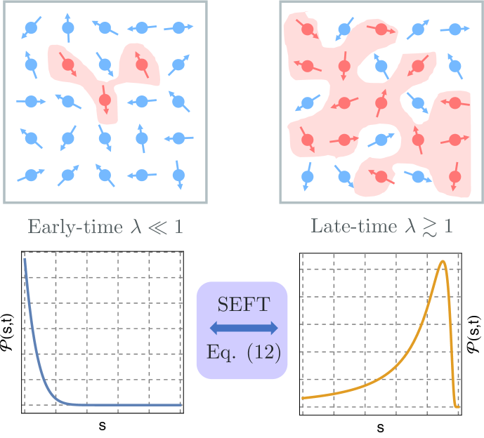
Figure 1: The schematics illustrate the consistency relation between the early-time operator size distribution and the late-time operator size distribution, valid under the assumption of SEFT.

In this work, motivated by these developments, we propose a scheme to test the validity of SEFT on quantum simulators. We focus on random spin models with all-to-all interactions, which has been realized in various experimental platforms. By generalizing the size-charge relation for Majorana systems, we derive the scramblon theory prediction of the operator size distribution in random spin models. The results show that the late-time operator size distribution can be predicted from its early-time value without any prior knowledge of $C$ or $\Upsilon^{m}_{O}$. This consistency relation serves as a smoking gun for the SEFT. As an illustration, we apply our scheme to Brownian circuits Zhou and Chen (2019), where the operator size distribution can be efficiently simulated by solving classical differential equations. Both analytical and numerical results confirm the validity of its SEFT description. We also discuss the prediction of multiple-quantum coherence (MQC) when the SEFT is valid. Our result is of fundamental interest for understanding the scrambling dynamics in generic quantum systems.

Operator size & total spin.– We focus on systems of $N$ spins $\hat{\bm{s}}^{j}=\hat{\bm{\sigma}}^{j}/2$ with time-reversal-invariant all-to-all interactions. Here $j=$1, 2, …, $N$ labels different spins. Protocols without the time-reversal symmetry are discussed in later. An Hermitian operator $\hat{O}(t)$ can be expanded using the complete basis of Pauli operators

$$\hat{O}(t)=\sum_{n}\sum_{j_{1}<\cdots<j_{n}}\sum_{\alpha_{1}\cdots\alpha_{n}}C_{j_{1}\alpha_{1}\cdots j_{n}\alpha_{n}}\hat{\sigma}_{\alpha_{1}}^{j_{1}}\hat{\sigma}_{\alpha_{2}}^{j_{2}}\cdots\hat{\sigma}_{\alpha_{n}}^{j_{n}},$$ (3)

where $\alpha_{k}\in\{x,y,z\}$ labels different Pauli matrices. The length $n$ of $\sigma_{\alpha_{1}}^{j_{1}}\cdots\sigma_{\alpha_{n}}^{j_{n}}$ is defined as the size of this basis. The operator size distribution $P(n,t)$ counts the operator weight on bases with size $n$ as

$$P(n,t)=\sum_{j_{1}<\cdots<j_{n}}\sum_{\alpha_{1}\cdots\alpha_{n}}(C_{j_{1}\alpha_{1}\cdots j_{n}\alpha_{n}})^{2},$$ (4)

with $n\in\{1,2,...,N\}$. The total probability is then conserved $\sum_{n}P(n,t)=1$ due to the unitarity if we normalize $\langle\hat{O}^{2}\rangle=1$. In the thermodynamic limit $N\gg 1$, we further introduce a continuous variable $s=n/N\in[0,1]$ with continuous distribution $\mathcal{P}(s,t)\equiv NP(sN,t)$, which is normalized as $\int_{0}^{1}ds~{}\mathcal{P}(s,t)=1$.

In Ref. Qi and Streicher (2019), the authors establish a connection between the operator size in Majorana systems and the charge operator in the doubled system. This formulation enables a systematic investigation of the distribution of operator sizes within the framework of the SEFT. We present a generalization of this relation to spin models. We first introduce an auxiliary system consisting of $N$ spins $\hat{\bm{s}}^{\prime j}=\hat{\bm{\tau}}^{j}/2$. The doubled system is prepared in the tensor product of singlet states $|\text{EPR}\rangle=\prod_{\otimes j}|\text{S}\rangle_{j}=\prod_{\otimes j}(\ket{\uparrow}_{\sigma^{j}}\ket{\downarrow}_{\tau^{j}}-\ket{\downarrow}_{\sigma^{j}}\ket{\uparrow}_{\tau^{j}})$. Consequently, we have $\hat{\bm{s}}^{j}_{\text{tot}}|\text{EPR}\rangle=(\hat{\bm{s}}^{\prime j}+\hat{\bm{s}}^{j})|\text{EPR}\rangle=0$. To study the size of an operator $\hat{O}(t)$, we map the operator to a state by $|O(t)\rangle=O(t)|\text{EPR}\rangle$ Qi and Streicher (2019). The Eq. (3) then becomes an expansion in orthonormal states. The crucial observation is

$$|\text{T},\alpha\rangle_{j}\equiv\hat{\sigma}^{j}_{\alpha}|\text{S}\rangle_{j},\ \ \ \ \ (\hat{\bm{s}}^{j}_{\text{tot}})^{2}|\text{T},\alpha\rangle_{j}=2|\text{T},\alpha\rangle_{j}.$$ (5)

Here, T indicates that the state is a spin-triplet. From a group theoretical perspective, this is due to $\hat{\sigma}^{j}_{\alpha}$ being a spin-$1$ spherical tensor operator. Consequently, the size of a string of Pauli operators is equal to the number of triplet states, counting over different site $j$. This gives

$$\mathcal{P}(s,t)=\langle\hat{O}(t)|\delta(s-\sum_{j}(\hat{\bm{s}}^{j}_{\text{tot}})^{2}/2N)|\hat{O}(t)\rangle.$$ (6)

When calculating the operator size distribution, it is more convenient to introduce the generating function $\mathcal{S}(\nu,t)=\int ds~{}\mathcal{P}(s,t)e^{-\nu s}$. Using Eq. (6), we find

$$\mathcal{S}(\nu,t)=e^{-\frac{3\nu}{4}}\langle\hat{O}(t)|e^{-\frac{\nu}{4N}\sum_{j}\bm{\sigma}^{j}\cdot\bm{\tau}^{j}}|\hat{O}(t)\rangle.$$ (7)

Note that Eq. (6) and Eq. (7) not only serve as a starting point for theoretical calculations but also provide a concrete protocol for measuring the operator size distribution on quantum simulators. This protocol requires the ability to prepare the initial EPR state and reverse the Hamiltonian, which are feasible with state-of-the-art cold atom systems and superconducting qubits.

(a) General diagram for $\mathcal{S}(\nu,t)$	(b) The early-time limit $(\lambda\ll 1)$

Figure 2: Typical diagrams of $\mathcal{S}(\nu,t)$ are shown in (a) for the full time range and (b) in the early-time limit $\lambda\ll 1$. Wavy lines represent the propagator of scrambling modes, while solid lines represent the microscopic operators $\hat{O}(t)$ or $\hat{\sigma}^{j}_{\alpha}$. The vertices within the dashed red circle become identical for $\hat{O}=\hat{\sigma}^{j_{1}}_{\alpha_{1}}$, indicating a consistency relation between different time regimes.

SEFT calculation.– Assuming the validity of the scramblon description, the generating function $\mathcal{S}(\nu,t)$ can be computed in closed-form. Performing the Taylor expansion of (7), the result contains general OTOCs between $\hat{O}$ and Pauli strings

$$\mathcal{S}=e^{-\frac{3\nu}{4}}\sum_{m}\left(\frac{\nu}{4N}\right)^{m}\sum_{\{j_{k},\alpha_{k}\}}\langle\hat{O}(t)\hat{\sigma}^{j_{1}}_{\alpha_{1}}...\hat{\sigma}^{j_{m}}_{\alpha_{m}}\hat{O}(t)\hat{\sigma}^{j_{1}}_{\alpha_{1}}...\hat{\sigma}^{j_{m}}_{\alpha_{m}}\rangle.$$ (8)

We have neglected contributions from collision terms where $j_{k}=j_{k^{\prime}}$, which become negligible in the thermodynamic limit $N\rightarrow\infty$. In the SEFT picture, each pair of $\sigma^{j_{k}}_{\alpha_{k}}$ operators can emit an arbitrary number of scramblons, all of which are ultimately absorbed by $\hat{O}$ operators in the future. A typical diagram with $m=3$ is shown in FIG. 2 (a). By summing up all possible configurations, result can be expressed as

$$\mathcal{S}=e^{-\frac{3\nu}{4}}\sum_{m}\frac{1}{m!}\left(\frac{\nu}{4}\right)^{m}\sum_{\{n_{k},\alpha_{k}\}}\frac{(-\lambda)^{\sum_{m}{n_{m}}}}{m!}\Upsilon^{\sum_{m}{n_{m}}}_{O}\Upsilon_{\alpha_{1}}^{n_{1}}...\Upsilon_{\alpha_{m}}^{n_{m}}.$$ (9)

Here, we define averaged vertex functions as $\Upsilon_{\alpha}^{m}\equiv\sum_{j}\Upsilon_{\sigma^{j}_{\alpha}}^{m}/N$ for conciseness. In comparison to the results for Majorana fermions Zhang and Gu (2022); Zhang and Yu (2022), we need to include an additional summation over $\alpha$ to account for the contributions from different Pauli matrices. By utilizing Eq. (2), we can perform the summation and obtain

$$\mathcal{S}(\nu,t)=\int_{0}^{\infty}dy~{}h_{O}(y)e^{-\frac{\nu}{4}({3}-\sum_{\alpha}f_{\alpha}(\lambda y))},$$ (10)

where we have $f_{O}(x)\equiv\sum_{m}(-x)^{m}\Upsilon_{O}^{m}/m!=\int dy~{}h_{O}(y)e^{-xy}$ describing the perturbed two-point functions with scramblon fields Gu et al. (2022). The operator size distribution can then be obtained by taking the inverse Laplace transform $\mathcal{P}(s,t)=\int_{0}^{\infty}dy~{}h_{O}(y)~{}\delta\Big{(}s-\frac{{3}-\sum_{\alpha}f_{\alpha}(\lambda y)}{4}\Big{)}.$

Consistency relation.– We are ready to show that Eq. (10) indicates non-trivial consistency relation of the operator size distribution when the SEFT description is valid. We take an average of $\mathcal{\mathcal{P}}(s,t)$ over single Pauli operators $\hat{O}=\hat{\sigma}^{j}_{\alpha}$

$$\overline{\mathcal{P}}(s,t)=\int_{0}^{\infty}dy~{}\overline{h}(y)\delta\Big{(}s-s_{\text{sc}}({{1}-\overline{f}(\lambda y))}\Big{)},$$ (11)

with $\overline{g}(x)\equiv\sum_{\alpha}g_{\alpha}(x)/3\equiv\sum_{\alpha,j}g_{\sigma_{\alpha}^{j}}(x)/3N$. For systems in which different spins are equivalent, the averaging over $j$ can be omitted. $s_{\text{sc}}=3/4$ is the typical size for a maximally scrambled operator in spin models, where all possible operators appear with equal probability. This can be seen by taking $\lambda\rightarrow\infty$ in Eq. (11), which gives $\overline{\mathcal{P}}(s,\infty)=\delta(s-s_{\text{sc}})$ for chaotic models with $\overline{f}(\infty)=0$ Gu et al. (2022). It is worth noting that a similar expression holds for systems with Majorana fermions Zhang and Gu (2022), with $s_{\text{sc}}=1/2$. Therefore, the consistency relation derived in this section can also be applied to Majorana systems.

The key observation is that the averaged generating function at different times $\nu$ and $t$ relies solely on a single function $\overline{h}(y)$, as $\overline{f}(x)$ is its Laplace transform. Our strategy is to first express $\overline{h}(y)$ in terms of the early-time size distribution with $N^{-1}\ll\lambda\ll 1$, and then establish its relation to the distribution at late times. A diagrammatic illustration is presented in FIG. 2. In the early-time regime with $N^{-1}\ll\lambda_{0}=e^{\varkappa t_{0}}/C\ll 1$, we expand $\overline{f}(\lambda_{0}y)=1-\lambda_{0}y\overline{\Upsilon}^{1}$. Using Eq. (11), we find

$$\overline{\mathcal{P}}(s,t_{0}) =({s_{\text{sc}}\lambda_{0}\overline{\Upsilon}^{1}})^{-1}\overline{h}\Big{(}s({s_{\text{sc}}\lambda_{0}\overline{\Upsilon}^{1}})^{-1}\Big{)},$$ (12)

$$\overline{s_{0}} =\int_{0}^{1}ds~{}s~{}\overline{\mathcal{P}}(s,t_{0})=s_{\text{sc}}\lambda_{0}(\overline{\Upsilon}^{1})^{2}.$$

The main obstacle in extracting $\overline{h}(y)$ from $\overline{\mathcal{P}}(s,t_{0})$ lies in the unknown coefficients $C$ and $\overline{\Upsilon}^{1}$. Fortunately, these coefficients ultimately cancel out, resulting in no free parameters in the consistency relation. To demonstrate this, let us consider the distribution (11) for a general time $\lambda$. By introducing $y=s_{1}/({s_{\text{sc}}\lambda_{0}\overline{\Upsilon}^{1}})$, it becomes straightforward to show that ¯P(s,t)=∫0∞ds1¯P(s1,t0)δ(s-ssc+ssc∫0∞ds2¯P(s2,t0)exp(-s1s2ssc¯s0eϰ(t-t0))). This is the main result for this work. Note that we can safely extend the integral to $[0,\infty]$ since the early-time distribution $\overline{\mathcal{P}}(s,t_{0})$ is only support near $s\ll 1$. Since (Signature of Scramblon Effective Field Theory in Random Spin Models) should be valid for arbitrary $s$ and $t$, it is highly restrictive and serves as a signature of SEFT in systems with all-to-all interactions. Eq. (Signature of Scramblon Effective Field Theory in Random Spin Models) can also be applied to predict the averaged operator size

$$\frac{\overline{s}}{s_{\text{sc}}}=1-\int_{0}^{\infty}\mathrm{d}s_{1}ds_{2}\overline{\mathcal{P}}(s_{1},t_{0})\overline{\mathcal{P}}(s_{2},t_{0})e^{-\frac{s_{1}s_{2}}{s_{\text{sc}}\overline{s_{0}}}e^{\varkappa(t-t_{0})}}.$$ (13)

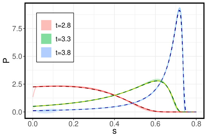
Figure 3: The operator size distribution of the Brownian circuits is shown for $N=10^{4}$. In this plot, different colors correspond to different times $t$. The dashed lines represent the results obtained from numerical simulations, while the solid lines depict the analytical solution given by Eq. (16). The region shaded with light color is obtained by numerically evaluating the integral in (Signature of Scramblon Effective Field Theory in Random Spin Models) for various $t_{0}$ values, while ensuring that $\overline{s_{0}}/s_{\text{sc}}\in[0.03,0.05]$.

Protocol: We summarize the concrete experimental protocol to test the validity of the SEFT on quantum simulators:

Step 1: Perform measurements of the operator size distribution $\mathcal{P}(s,t)_{\text{exp}}$ for different times $t$ with $\hat{O}=\hat{\sigma}^{j}_{\alpha}$, following the size-total spin relation or other existing protocols Qi et al. (2019); Blocher et al. (2023). Compute the averaged distribution $\overline{\mathcal{P}}(s,t)_{\text{exp}}$ over sites $j$ and $\alpha\in\{x,y,z\}$.

Step 2: Choose a set of ${t_{0}^{k}}$ with $t_{0}^{k}\ll\log N$, compute the averaged operator size $\overline{s_{0}}$, and extract $\varkappa$ by performing a linear fit of the averaged size $\log\overline{s_{0}}$ for different $t_{0}$ values.

Step 3: Select a specific $t_{0}\ll\log N$, compute the numerical integral in Eq. (Signature of Scramblon Effective Field Theory in Random Spin Models) using the experimental result $\overline{\mathcal{P}}(s,t_{0})_{\text{exp}}$ for a general time $t$ to obtain the theoretical prediction $\overline{\mathcal{P}}(s,t)_{\text{th}}$. Compare this prediction with the experimental data $\overline{\mathcal{P}}(s,t)_{\text{exp}}$.

We finally address the generalization to systems without time-reversal symmetry or at finite temperatures. (i). In the absence of time-reversal symmetry, the vertices for absorbing scramblons in the future and emitting scramblons in the past become distinct, denoted as $\Upsilon^{\text{R},m}$ and $\Upsilon^{\text{A},m}$, respectively. Similarly, the labels R$/$A should be added to the functions $f_{O}^{\text{R/A}}$ and $h_{O}^{\text{R/A}}$. Consequently, we can only determine the operator size at late-time $t\gg t_{\text{sc}}$ by combining information of $\mathcal{P}(s,t_{0})$ and $\mathcal{P}(s,-t_{0})$. (ii). At finite temperatures, an unambiguous definition of the operator size distribution is lacking. To establish a relationship between the operator sizes in different time regimes, we adopt a specific definition. The operator size distribution of $\hat{O}(t)$ at an inverse temperature $\beta$ is defined as the standard operator size distribution of $\rho^{1/4}\hat{O}(t)\rho^{1/4}$, where $\rho=e^{-\beta\hat{H}}$ represents the thermal density matrix. Under this definition, an analog of (Signature of Scramblon Effective Field Theory in Random Spin Models) holds. We leave a detailed derivation into the supplementary material SM .

Example.– As an illustration, let us consider the Brownian circuits for spin-$1/2$ systems Zhou and Chen (2019). The Hamiltonian reads

$${H_{s}}\Delta t=J\sum_{i<j}\sum_{{\mu_{i}},{\mu_{j}}}\hat{\sigma}^{i}_{{\mu_{i}}}\hat{\sigma}^{j}_{{\mu_{j}}}\Delta B^{i,j}_{{\mu_{i}},{\mu_{j}}},$$ (14)

where $\mu_{i}\in\{0,x,y,z\}$. $\Delta B^{i,j}_{{\mu_{i}},{\mu_{j}}}$ represents independent Brownian variables with $(\Delta B^{i,j}_{{\mu_{i}},{\mu_{j}}})^{2}=\Delta t$. We take the normalization $J={({{{8}N}})^{-1/2}}$. The system exihibits the time-reversal symmetry. In Ref. Zhou and Chen (2019), the authors solved the operator size distribution of Brownian circuits by deriving a set of ordinary equations for $P(n,t)$ using Itô Calculus, which allows for efficient classical simulations with large $N$. However, due to the lack of a diagrammatic analysis, it remains unclear whether information scrambling in Brownian circuits can be described by the SEFT.

Here, we apply our protocol to Brownian circuits to address this question. In Brownian circuits, there is a permutation symmetry for different spins $j$ and different directions $\alpha$. As a result, the average can be omitted simplifying the analysis. The early-time operator size distribution $P(n,t)$ has been analytically computed in Zhou and Chen (2019). Taking the thermodynamic limit with fixed $e^{\varkappa t}/N$ and $\varkappa=3$, we discover

$$\overline{\mathcal{P}}(s,t_{0})=Ne^{-\varkappa t_{0}}\text{exp}\big{(}-sNe^{-\varkappa t_{0}}\big{)},\ \ \ \ \ \ \overline{s_{0}}=e^{\varkappa t_{0}}/N.$$ (15)

We then try to predict the operator size distribution for general time $t$ using (Signature of Scramblon Effective Field Theory in Random Spin Models) and (15). Performing the integration gives

$$\overline{\mathcal{P}}(s,t)=\frac{N}{(1-s/s_{\text{sc}})^{2}}\exp(-\varkappa t-\frac{sNe^{-\varkappa t}}{(1-s/s_{\text{sc}})}).$$ (16)

In FIG. 3, we compare this result to numerical simulations with $N={10^{4}}$. We find excellent agreement for arbitrary time $t$. This supports the validity of the SEFT in Brownian circuits. Interestingly, this formula has not been obtained explicitly within to our knowledge. Its moments match Eq. (20) in Zhou and Chen (2019) . For example, we have $\overline{s}/s_{\text{sc}}=1+ae^{a}\text{Ei}(-a)$ with $a=s_{\text{sc}}Ne^{-\varkappa t}$. For smaller $N$, we should take finite size corrections for Eq. (Signature of Scramblon Effective Field Theory in Random Spin Models) into account, as established in the supplementary material SM .

Up to now, we are using the analytical expression (15) for $\mathcal{P}(s,t_{0})$. However, the extraction of $\mathcal{P}(s,t_{0})$ contains additional continuous limit, which may lead to large error. We further test our protocol by direct application to numerical data of $P(n,t)$. We choose $t_{0}$ by fixing $\overline{s_{0}}/s_{\text{sc}}\in[0.03,0.05]$. The integral in (Signature of Scramblon Effective Field Theory in Random Spin Models) is performed numerically by using a Gaussian approximation of the Dirac delta function with standard deviation $\sigma={10^{-2}}$. The result for different $t_{0}$ is plotted in FIG. 3 as the shaded region, which is consistent with both numerics and analytical results (16).

MQC.– After confirming the validity of the SEFT in a specific model, we can proceed to make theoretical predictions for other experimental observables. As an example, we present results for the MQC, which is extensively studied in NMR experiments Abraham et al. (1998). To obtain MQC of $\hat{O}$, one first performs the measurement of

$$F(\varphi,t)=\langle e^{i\varphi\sum_{j}\hat{s}_{z}^{j}}\hat{O}(t)e^{-i\varphi\sum_{j}\hat{s}_{z}^{j}}\hat{O}(t)\rangle,\ \ \ \ \ \ \ \varphi\in[0,2\pi).$$ (17)

The MQC, denoted as $I(m,t)$, is defined as the Fourier transform of $F(\varphi,t)$ for integer values of $m$. In the thermodynamic limit $N\gg 1$, $F(\varphi,t)$ rapidly concentrates around $\varphi=0$ with a width on the order of $\sim{N}^{-\frac{1}{2}}$. To address this, we introduce the variable $\xi\equiv\sqrt{N}\varphi$ and $\mathcal{F}(\xi,t)\equiv F(\sqrt{N}\phi,t)$. The computation of $\mathcal{F}(\xi,t)$ can be done in a similar manner as for $\mathcal{S}(\nu,t)$ utilizing the SEFT. The resulting expression is

$$\mathcal{F}(\xi,t)=\int_{0}^{\infty}dy~{}h_{O}(y)e^{-\frac{\xi^{2}}{4}(1-f_{z}(\lambda y))}.$$ (18)

Unlike the operator size distribution, the MQC solely depends on $f_{z}$. By performing the Fourier transform $\mathcal{I}(u,t)=\int d\xi e^{iu\xi}\mathcal{F}(\xi,t)/2\pi$, the continuum limit of the MQC, denoted as $\mathcal{I}(u,t)$ with $u\equiv m/\sqrt{N}$, can be expressed as

$$\mathcal{I}(u,t)=\int_{0}^{\infty}dy~{}h_{O}(y)[\pi(1-f_{z}(\lambda y))]^{-1/2}e^{-\frac{u^{2}}{1-f_{z}(\lambda y)}}.$$ (19)

This can also be related to the operator size distribution at early times. For instance, if we consider $O=\hat{\sigma}^{j}_{z}$ and take an average over sites $j$, we can show that

$$\mathcal{I}_{z}(u,t)=\int_{0}^{\infty}ds_{1}~{}\mathcal{P}_{z}(s_{1},t_{0})[\pi(1-\mathcal{S}_{z}(\eta s_{1},t_{0}))]^{-1/2}e^{-\frac{u^{2}}{1-\mathcal{S}_{z}(\eta s_{1},t_{0})}},$$

where we have introduced $\eta(t,t_{0})={e^{\varkappa(t-t_{0})}}/{s_{\text{sc}}\overline{s_{0}}}$ for conciseness. The subscripts $z$ are included as a reminder.

Discussions.– In this work, we explore the signature of the SEFT in random spin models with all-to-all interactions. Our result (Signature of Scramblon Effective Field Theory in Random Spin Models) reveals a non-trivial consistency relation between the distribution of operator sizes in the early-time regime and their values at late-time. This finding serves as strong evidence for the validity of SEFT in a specific model, which can be experimentally tested on quantum simulator platforms. As an illustration, we apply the scheme to Brownian circuits, where a diagrammatic calculation is not available. Both analytical and numerical implements of our protocol confirms the validity of SEFT in Brownian circuits. We also present discussions for the MQC.

Recently, there are growing interest in quantum teleportation through emergent traversable wormholes Gao et al. (2017); Maldacena et al. (2017); Susskind and Zhao (2018); Gao and Liu (2019); Brown et al. (2019); Gao and Jafferis (2021); Nezami et al. (2021); Schuster et al. (2022), which has been experimentally investigated in Ref. Jafferis et al. (2022). The teleportation fidelity has been proposed to be associated with the size winding at finite temperatures. Our calculation can be generalized to establish a relationship between size winding in different time regimes for systems described by the SEFT. We would like to postpone a detailed study to future works.

Acknowledgement. We thank Xiao Chen, Yingfei Gu, Xinhua Peng and Tian-Gang Zhou for invaluable discussions.

See pages 1, of SI.pdf See pages 0, of SI.pdf

References

- Srednicki (1994) Mark Srednicki, “Chaos and quantum thermalization,” Phys. Rev. E 50, 888–901 (1994).
- Deutsch (1991) J. M. Deutsch, “Quantum statistical mechanics in a closed system,” Phys. Rev. A 43, 2046–2049 (1991).
- Hayden and Preskill (2007) Patrick Hayden and John Preskill, “Black holes as mirrors: Quantum information in random subsystems,” JHEP 09, 120 (2007), arXiv:0708.4025 [hep-th] .
- Sekino and Susskind (2008) Yasuhiro Sekino and Leonard Susskind, “Fast Scramblers,” JHEP 10, 065 (2008), arXiv:0808.2096 [hep-th] .
- Shenker and Stanford (2015) Stephen H. Shenker and Douglas Stanford, “Stringy effects in scrambling,” JHEP 05, 132 (2015), arXiv:1412.6087 [hep-th] .
- Roberts et al. (2015) Daniel A. Roberts, Douglas Stanford, and Leonard Susskind, “Localized shocks,” JHEP 03, 051 (2015), arXiv:1409.8180 [hep-th] .
- Nahum et al. (2018) Adam Nahum, Sagar Vijay, and Jeongwan Haah, “Operator Spreading in Random Unitary Circuits,” Phys. Rev. X 8, 021014 (2018), arXiv:1705.08975 [cond-mat.str-el] .
- von Keyserlingk et al. (2018) Curt von Keyserlingk, Tibor Rakovszky, Frank Pollmann, and Shivaji Sondhi, “Operator hydrodynamics, OTOCs, and entanglement growth in systems without conservation laws,” Phys. Rev. X 8, 021013 (2018), arXiv:1705.08910 [cond-mat.str-el] .
- Khemani et al. (2018) Vedika Khemani, Ashvin Vishwanath, and D. A. Huse, “Operator spreading and the emergence of dissipation in unitary dynamics with conservation laws,” Phys. Rev. X 8, 031057 (2018), arXiv:1710.09835 [cond-mat.stat-mech] .
- Hunter-Jones (2018) Nicholas Hunter-Jones, “Operator growth in random quantum circuits with symmetry,” (2018), arXiv:1812.08219 [quant-ph] .
- Chen and Lucas (2021) Chi-Fang Chen and Andrew Lucas, “Operator Growth Bounds from Graph Theory,” Commun. Math. Phys. 385, 1273–1323 (2021), arXiv:1905.03682 [math-ph] .
- Lucas (2019) Andrew Lucas, “Operator size at finite temperature and planckian bounds on quantum dynamics,” Phys. Rev. Lett. 122, 216601 (2019).
- Chen et al. (2020) Xiao Chen, Yingfei Gu, and Andrew Lucas, “Many-body quantum dynamics slows down at low density,” SciPost Phys. 9, 071 (2020), arXiv:2007.10352 [quant-ph] .
- Lucas and Osborne (2020) Andrew Lucas and Andrew Osborne, “Operator growth bounds in a cartoon matrix model,” J. Math. Phys. 61, 122301 (2020), arXiv:2007.07165 [hep-th] .
- Yin and Lucas (2021) Chao Yin and Andrew Lucas, “Quantum operator growth bounds for kicked tops and semiclassical spin chains,” Phys. Rev. A 103, 042414 (2021), arXiv:2010.06592 [cond-mat.str-el] .
- Zhou and Swingle (2021) Tianci Zhou and Brian Swingle, “Operator Growth from Global Out-of-time-order Correlators,” (2021), arXiv:2112.01562 [quant-ph] .
- Dias et al. (2021) Beatriz C. Dias, Masudul Haque, Pedro Ribeiro, and Paul McClarty, “Diffusive Operator Spreading for Random Unitary Free Fermion Circuits,” (2021), arXiv:2102.09846 [cond-mat.str-el] .
- Wu et al. (2021) Yadong Wu, Pengfei Zhang, and Hui Zhai, “Scrambling ability of quantum neural network architectures,” Physical Review Research 3, L032057 (2021), arXiv:2011.07698 [cond-mat.dis-nn] .
- Zhang and Yu (2022) Pengfei Zhang and Zhenhua Yu, “Dynamical Transition of Operator Size Growth in Open Quantum Systems,” (2022), arXiv:2211.03535 [quant-ph] .
- Zhang and Gu (2022) Pengfei Zhang and Yingfei Gu, “Operator Size Distribution in Large Quantum Mechanics of Majorana Fermions,” (2022), arXiv:2212.04358 [cond-mat.str-el] .
- Jian et al. (2021) Shao-Kai Jian, Brian Swingle, and Zhuo-Yu Xian, “Complexity growth of operators in the SYK model and in JT gravity,” JHEP 03, 014 (2021), arXiv:2008.12274 [hep-th] .
- Kitaev (2015) Alexei Kitaev, “A simple model of quantum holography,” (2015).
- Maldacena and Stanford (2016) Juan Maldacena and Douglas Stanford, “Remarks on the Sachdev-Ye-Kitaev model,” Phys. Rev. D 94, 106002 (2016), arXiv:1604.07818 [hep-th] .
- Kitaev and Suh (2018) Alexei Kitaev and S. Josephine Suh, “The soft mode in the Sachdev-Ye-Kitaev model and its gravity dual,” JHEP 05, 183 (2018), arXiv:1711.08467 [hep-th] .
- Chowdhury et al. (2022) Debanjan Chowdhury, Antoine Georges, Olivier Parcollet, and Subir Sachdev, “Sachdev-ye-kitaev models and beyond: Window into non-fermi liquids,” Rev. Mod. Phys. 94, 035004 (2022).
- Gu et al. (2022) Yingfei Gu, Alexei Kitaev, and Pengfei Zhang, “A two-way approach to out-of-time-order correlators,” JHEP 03, 133 (2022), arXiv:2111.12007 [hep-th] .
- Gu and Kitaev (2019) Yingfei Gu and Alexei Kitaev, “On the relation between the magnitude and exponent of OTOCs,” JHEP 02, 075 (2019), arXiv:1812.00120 [hep-th] .
- Zhang (2023) Pengfei Zhang, “Information scrambling and entanglement dynamics of complex Brownian Sachdev-Ye-Kitaev models,” JHEP 04, 105 (2023), arXiv:2301.03189 [cond-mat.str-el] .
- (29) Tian-Gang Zhou, Pengfei Zhang, and Yingfei Gu, In Preparation .
- (30) Pengfei Zhang, Alexei Kitaev, and Yingfei Gu, In Preparation .
- Islam et al. (2015) Rajibul Islam, Ruichao Ma, Philipp M. Preiss, M. Eric Tai, Alexander Lukin, Matthew Rispoli, and Markus Greiner, “Measuring entanglement entropy in a quantum many-body system,” Nature (London) 528, 77–83 (2015), arXiv:1509.01160 [cond-mat.quant-gas] .
- Li et al. (2017) Jun Li, Ruihua Fan, Hengyan Wang, Bingtian Ye, Bei Zeng, Hui Zhai, Xinhua Peng, and Jiangfeng Du, “Measuring Out-of-Time-Order Correlators on a Nuclear Magnetic Resonance Quantum Simulator,” Phys. Rev. X 7, 031011 (2017), arXiv:1609.01246 [cond-mat.str-el] .
- Gärttner et al. (2017) Martin Gärttner, Justin G. Bohnet, Arghavan Safavi-Naini, Michael L. Wall, John J. Bollinger, and Ana Maria Rey, “Measuring out-of-time-order correlations and multiple quantum spectra in a trapped ion quantum magnet,” Nature Phys. 13, 781 (2017), arXiv:1608.08938 [quant-ph] .
- Brydges et al. (2019) Tiff Brydges, Andreas Elben, Petar Jurcevic, Benoît Vermersch, Christine Maier, Ben P. Lanyon, Peter Zoller, Rainer Blatt, and Christian F. Roos, “Probing Rényi entanglement entropy via randomized measurements,” Science 364, 260–263 (2019), arXiv:1806.05747 [quant-ph] .
- Sánchez et al. (2019) Claudia M. Sánchez, Ana Karina Chattah, Ken Xuan Wei, Lisandro Buljubasich, Paola Cappellaro, and Horacio M. Pastawski, “Emergent perturbation independent decay of the Loschmidt echo in a many-spin system studied through scaled dipolar dynamics,” arXiv e-prints , arXiv:1902.06628 (2019), arXiv:1902.06628 [quant-ph] .
- Landsman et al. (2019) K. A. Landsman, C. Figgatt, T. Schuster, N. M. Linke, B. Yoshida, N. Y. Yao, and C. Monroe, “Verified quantum information scrambling,” Nature (London) 567, 61–65 (2019), arXiv:1806.02807 [quant-ph] .
- Joshi et al. (2020) Manoj K. Joshi, Andreas Elben, Benoît Vermersch, Tiff Brydges, Christine Maier, Peter Zoller, Rainer Blatt, and Christian F. Roos, “Quantum Information Scrambling in a Trapped-Ion Quantum Simulator with Tunable Range Interactions,” Phys. Rev. Lett. 124, 240505 (2020), arXiv:2001.02176 [quant-ph] .
- Blok et al. (2021) M. S. Blok, V. V. Ramasesh, T. Schuster, K. O’Brien, J. M. Kreikebaum, D. Dahlen, A. Morvan, B. Yoshida, N. Y. Yao, and I. Siddiqi, “Quantum Information Scrambling on a Superconducting Qutrit Processor,” Phys. Rev. X 11, 021010 (2021), arXiv:2003.03307 [quant-ph] .
- Domínguez et al. (2021) Federico D. Domínguez, María Cristina Rodríguez, Robin Kaiser, Dieter Suter, and Gonzalo A. Álvarez, “Decoherence scaling transition in the dynamics of quantum information scrambling,” Phys. Rev. A 104, 012402 (2021), arXiv:2005.12361 [quant-ph] .
- Domínguez and Álvarez (2021) Federico D. Domínguez and Gonzalo A. Álvarez, “Dynamics of quantum information scrambling under decoherence effects measured via active spin clusters,” Phys. Rev. A 104, 062406 (2021), arXiv:2107.03870 [quant-ph] .
- Mi et al. (2021) Xiao Mi et al., “Information scrambling in quantum circuits,” Science 374, abg5029 (2021), arXiv:2101.08870 [quant-ph] .
- Cotler et al. (2022) Jordan Cotler, Thomas Schuster, and Masoud Mohseni, “Information-theoretic Hardness of Out-of-time-order Correlators,” (2022), arXiv:2208.02256 [quant-ph] .
- Sánchez et al. (2022) C. M. Sánchez, A. K. Chattah, and H. M. Pastawski, “Emergent decoherence induced by quantum chaos in a many-body system: A Loschmidt echo observation through NMR,” Phys. Rev. A 105, 052232 (2022), arXiv:2112.00607 [quant-ph] .
- Qi et al. (2019) Xiao-Liang Qi, Emily J. Davis, Avikar Periwal, and Monika Schleier-Smith, “Measuring operator size growth in quantum quench experiments,” (2019), arXiv:1906.00524 [quant-ph] .
- Zhou and Chen (2019) Tianci Zhou and Xiao Chen, “Operator dynamics in a Brownian quantum circuit,” Phys. Rev. E 99, 052212 (2019), arXiv:1805.09307 [cond-mat.str-el] .
- Qi and Streicher (2019) Xiao-Liang Qi and Alexandre Streicher, “Quantum Epidemiology: Operator Growth, Thermal Effects, and SYK,” JHEP 08, 012 (2019), arXiv:1810.11958 [hep-th] .
- Blocher et al. (2023) Philip Daniel Blocher, Karthik Chinni, Sivaprasad Omanakuttan, and Pablo M. Poggi, “Probing scrambling and operator size distributions using random mixed states and local measurements,” (2023), arXiv:2305.16992 [quant-ph] .
- (48) See supplementary material for: (i). Detailed derivation of operator size without time-reversal symmetry or at finite temperature; (ii). Numerics for the Brownian circuit model; (iii). Finite size correction.
- Abraham et al. (1998) Raymond John Abraham, Julie Fisher, and Philip Loftus, Introduction to NMR spectroscopy, Vol. 2 (Wiley New York, 1998).
- Gao et al. (2017) Ping Gao, Daniel Louis Jafferis, and Aron C. Wall, “Traversable Wormholes via a Double Trace Deformation,” JHEP 12, 151 (2017), arXiv:1608.05687 [hep-th] .
- Maldacena et al. (2017) Juan Maldacena, Douglas Stanford, and Zhenbin Yang, “Diving into traversable wormholes,” Fortsch. Phys. 65, 1700034 (2017), arXiv:1704.05333 [hep-th] .
- Susskind and Zhao (2018) Leonard Susskind and Ying Zhao, “Teleportation through the wormhole,” Phys. Rev. D 98, 046016 (2018), arXiv:1707.04354 [hep-th] .
- Gao and Liu (2019) Ping Gao and Hong Liu, “Regenesis and quantum traversable wormholes,” JHEP 10, 048 (2019), arXiv:1810.01444 [hep-th] .
- Brown et al. (2019) Adam R. Brown, Hrant Gharibyan, Stefan Leichenauer, Henry W. Lin, Sepehr Nezami, Grant Salton, Leonard Susskind, Brian Swingle, and Michael Walter, “Quantum Gravity in the Lab: Teleportation by Size and Traversable Wormholes,” (2019), arXiv:1911.06314 [quant-ph] .
- Gao and Jafferis (2021) Ping Gao and Daniel Louis Jafferis, “A traversable wormhole teleportation protocol in the SYK model,” JHEP 07, 097 (2021), arXiv:1911.07416 [hep-th] .
- Nezami et al. (2021) Sepehr Nezami, Henry W. Lin, Adam R. Brown, Hrant Gharibyan, Stefan Leichenauer, Grant Salton, Leonard Susskind, Brian Swingle, and Michael Walter, “Quantum Gravity in the Lab: Teleportation by Size and Traversable Wormholes, Part II,” (2021), arXiv:2102.01064 [quant-ph] .
- Schuster et al. (2022) Thomas Schuster, Bryce Kobrin, Ping Gao, Iris Cong, Emil T. Khabiboulline, Norbert M. Linke, Mikhail D. Lukin, Christopher Monroe, Beni Yoshida, and Norman Y. Yao, “Many-body quantum teleportation via operator spreading in the traversable wormhole protocol,” Phys. Rev. X 12, 031013 (2022).
- Jafferis et al. (2022) Daniel Jafferis, Alexander Zlokapa, Joseph D. Lykken, David K. Kolchmeyer, Samantha I. Davis, Nikolai Lauk, Hartmut Neven, and Maria Spiropulu, “Traversable wormhole dynamics on a quantum processor,” Nature 612, 51–55 (2022).