$B\to D^{*}\ell{\nu_{\ell}}$ semileptonic form factors from lattice QCD with Möbius domain-wall quarks

Abstract

We calculate the form factors for the $B\!\to\!D^{*}\ell{\nu_{\ell}}$ decay in 2+1 flavor lattice QCD. For all quark flavors, we employ the Möbius domain-wall action, which preserves chiral symmetry to a good precision. Our gauge ensembles are generated at three lattice cutoffs $a^{-1}\sim 2.5$, 3.6 and 4.5 GeV with pion masses as low as $M_{\pi}\!\sim\!230$ MeV. The physical lattice size $L$ satisfies the condition $M_{\pi}L\geq 4$ to control finite volume effects (FVEs), while we simulate a smaller size at the smallest $M_{\pi}$ to directly examine FVEs. The bottom quark masses are chosen in a range from the physical charm quark mass to 0.7 $a^{-1}$ to control discretization effects. We extrapolate the form factors to the continuum limit and physical quark masses based on heavy meson chiral perturbation theory at next-to-leading order. Then the recoil parameter dependence is parametrized using a model independent form leading to our estimate of the decay rate ratio between the tau ($\ell\!=\!\tau$) and light lepton ($\ell\!=\!e,\mu$) channels $R(D^{*})\!=\!0.252(22)$ in the Standard Model. A simultaneous fit with recent data from the Belle experiment yields $|V_{cb}|\!=\!39.19(90)\times 10^{-3}$, which is consistent with previous exclusive determinations, and shows good consistency in the kinematical distribution of the differential decay rate between the lattice and experimental data.

I Introduction

The $B\!\to\!D^{*}\ell{\nu_{\ell}}$ semileptonic decay, where $\ell\!=\!e,\mu,\tau$ and ${\nu_{\ell}}$ represents the corresponding neutrino, plays a key role in stringent tests of the Standard Model (SM) and searches for new physics. The channels associated with light leptons $\ell\!=\!e,\mu$ provide a determination of the Cabibbo-Kobayashi-Maskawa (CKM) matrix element ${|V_{cb}|}$, which is a fundamental parameter of the SM. On the other hand, the $\tau$ channel is expected to be a good probe of new physics, since, for instance, it is expected to strongly couple to the charged Higgs boson predicted by supersymmetric models. Indeed, there is an intriguing $\gtrsim\!3\,\sigma$ tension between the SM and experiments on the decay rate ratio

$$R(D^{*}) = \frac{\Gamma(B\!\to\!D^{*}\tau\nu_{\tau})}{\Gamma(B\!\to\!D^{*}\ell{\nu_{\ell}})}\hskip 14.22636pt(\ell=e,\mu)$$ (1)

describing the lepton-flavor universality violation Amhis et al. (2023).

However, there has been a long-standing tension between the $|V_{cb}|$ determinations from exclusive and inclusive decays $(B\!\to\!D\ell{\nu_{\ell}}+D^{*}\ell{\nu_{\ell}}+D^{**}\ell{\nu_{\ell}}+\cdots)$. The Heavy Flavor Averaging Group reported that analysis of the inclusive decay yields Amhis et al. (2023)

$${|V_{cb}|}\times 10^{3} = 41.98(45),$$ (2)

which shows a $\lesssim\!4\,\sigma$ (9 %) tension with the determination from the exclusive decays

$${|V_{cb}|}\times 10^{3} = \left\{\begin{array}[]{ll}39.14(99)&(B\!\to\!D\ell{\nu_{\ell}}),\\ 38.46(68)&(B\!\to\!D^{*}\ell{\nu_{\ell}}).\end{array}\right.$$ (5)

It has been argued Crivellin and Pokorski (2015) that such a tension can be explained by introducing a tensor interaction beyond the SM, which, however, largely distorts the $Z\!\to\!\bar{b}b$ decay rate measured precisely by experiments. Therefore, it is likely that the ${|V_{cb}|}$ tension is due to our incomplete understanding of the theoretical and/or experimental uncertainty.

The largest theoretical uncertainty in the exclusive determination comes from form factors, which describe non-perturbative QCD effects to the decay amplitude through the matrix elements

$$\sqrt{M_{B}M_{D^{*}}}^{-1}\langle D^{*}({\epsilon^{\prime}},{p^{\prime}})|V_{\mu}|B(p)\rangle = i\varepsilon_{\mu\nu\rho\sigma}\,{\epsilon^{\prime}}^{\nu}v^{\prime\rho}v^{\sigma}\,h_{V}(w),$$ (6)

$$\sqrt{M_{B}M_{D^{*}}}^{-1}\langle D^{*}({\epsilon^{\prime}},{p^{\prime}})|A_{\mu}|B(p)\rangle = (w+1)\,\epsilon_{\mu}^{\prime*}\,h_{A_{1}}(w)-({\epsilon^{\prime*}}v)\left\{v_{\mu}\,h_{A_{2}}(w)+{v^{\prime}}_{\mu}\,h_{A_{3}}(w)\right\},\hskip 28.45274pt$$ (7)

where $w=v{v^{\prime}}$ is the recoil parameter defined by four velocities $v\!=\!p/M_{B}$ and ${v^{\prime}}\!=\!{p^{\prime}}/M_{D^{(*)}}$, and ${\epsilon^{\prime}}$ is the polarization vector of $D^{*}$, which satisfies ${p^{\prime}}{\epsilon^{\prime}}\!=\!0$. Note that, here and in the following, kinematical variables (momentum, velocity, polarization vector, but not space-time coordinates) with and without the symbol “$\prime$” represent those for $D^{*}$ and $B$, respectively.

Lattice QCD is a powerful method to provide a first-principles calculation of the form factors with systematically improvable accuracy Vaquero (2022); Kaneko (2023). However, until recently, only $h_{A_{1}}(1)$ at the zero-recoil limit $w=1$ had been calculated in unquenched lattice QCD Bernard et al. (2009); Bailey et al. (2014); Harrison et al. (2018). In the previous determination of ${|V_{cb}|}$, therefore, other information of the form factors in addition to ${|V_{cb}|}$ had to be determined by fitting experimental data of the differential decay rate to a theoretical expression Amhis et al. (2023); Bernlochner et al. (2017); Bigi et al. (2017a); Grinstein and Kobach (2017). While a model independent parametrization of the form factors by Boyd, Grinstein and Lebed (the BGL parametrization) is available Boyd et al. (1997), its large number of parameters due to the poor knowledge on the form factors makes the fit unstable Bigi et al. (2017b); Bernlochner et al. (2019); Gambino et al. (2019); Ferlewicz et al. (2021) even with experimental data of differential distribution with respect to all kinematical variables, namely the recoil parameter and three decay angles, from the KEKB/Belle experiment Waheed et al. (2019); Abdesselam et al. (2017) .

One of the largest problems in the lattice study of $B$ meson physics is that the simulation cost rapidly increases as the lattice spacing decreases. In spite of recent progress in computer performance and development of simulation algorithms, it is still difficult to simulate lattice cutoffs $a^{-1}$ sufficiently larger than the physical bottom quark mass ${m_{b,\rm phys}}$ to suppress $O((am_{b})^{n})$ discretization errors to, say, the 1 % level. For the time being, a practical approach to $B$ physics on the lattice is to employ a heavy quark action based on an effective field theory, such as the heavy quark effective theory (HQET), to directly simulate ${m_{b,\rm phys}}$ at currently available cutoffs $a^{-1}\!\lesssim\!{m_{b,\rm phys}}$. Another straightforward approach is the so-called relativistic approach, where a lattice QCD action is used also for heavy quarks but with their masses sufficiently smaller than the lattice cutoff to suppress discretization effects. The Fermilab/MILC reported the first lattice calculation of all form factors at zero and non-zero recoils Bazavov et al. (2022) using the Fermilab approach for heavy quarks, namely a HQET interpretation of the anisotropic Wilson-clover quark action El-Khadra et al. (1997), and staggered light quarks. It was recently followed by the HPQCD Collaboration with a fully relativistic approach Harrison and Davies (2023), where the highly improved staggered quark action was used both for light and heavy flavors.

In this paper, we present an independent study with a fully relativistic approach using the Möbius domain-wall quark action Brower et al. (2017) for all relevant quark flavors. This preserves chiral symmetry to good precision at finite lattice spacing, reducing the leading discretization errors to second order, i.e. $O((am_{b})^{2})$. We can also use chiral perturbation theory in the continuum limit ($a\!=\!0$) to guide the chiral extrapolation to the physical pion mass. Note also that we do not need explicit renormalization of the weak axial and vector currents on the lattice to calculate relevant form factors, because the renormalization constants of these currents coincide with each other and are canceled by taking appropriate ratios of relevant correlation functions Hashimoto et al. (1999). Our preliminary analyses and discussions on these features can be found in our earlier reports Kaneko et al. (2018, 2019, 2022).

This paper is organized as follows. After a brief introduction to our choice of simulation parameters, the form factors are extracted from correlation functions at the simulation points in Sec. II. These results are extrapolated to the continuum limit and physical quark masses in Sec. III. In Sec. IV, we generate synthetic data of the form factors and fit them to a model-independent parametrization in terms of the recoil parameter to make a comparison with the previous lattice and phenomenological studies as well as to estimate the SM value of $R(D^{*})$. We also perform a simultaneous fit with experimental data to estimate $|V_{cb}|$. Our conclusions are given in Sec. V.

II Form factors at simulation points

II.1 Gauge ensembles

Our gauge ensembles are generated for 2+1-flavor lattice QCD, where dynamical up and down quarks are degenerate and dynamical strange quark has a distinct mass. We take three lattice spacings of $a\!\simeq\!0.044,0.055$ and 0.080 fm Colquhoun et al. (2022), which correspond to the lattice cutoffs $a^{-1}\sim 2.453(4)$, 3.610(9) and 4.496(9) GeV, respectively. They are determined using the Yang-Mills gradient flow Borsanyi et al. (2012). The tree-level improved Symanzik gauge action Weisz (1983); Weisz and Wohlert (1984); Luscher and Weisz (1985) and the Möbius domain-wall quark action Brower et al. (2017) are used to control discretization errors and to preserve chiral symmetry to a good precision. We refer the interested reader to Refs. Brower et al. (2017); Colquhoun et al. (2022); Boyle (2015) for the five dimensional formulation of the quark action and our implementation. Its four-dimensional effective Dirac operator is given by

$$\frac{1+m_{q}}{2}+\frac{1-m_{q}}{2}\gamma_{5}\,\epsilon\left[H_{M}\right],$$ (8)

where $m_{q}$ represents the quark mass. We employ the kernel operator $H_{M}\!=\!2\gamma_{5}D_{W}(-M)/\left\{2+D_{W}(-M)\right\}$, where $D_{W}(-M)$ is the Wilson-Dirac operator with a negative mass with $M\!=\!1$ and with stout smearing Morningstar and Peardon (2004) applied three successive times to the gauge links. The polar decomposition approximation is realized for the sign function $\epsilon\left[H_{M}\right]$ in the five-dimensional domain-wall implementation. With this choice, the residual quark mass, which is a measure of the chiral symmetry violation, is suppressed to the level of 1 MeV at $a\!\simeq\!0.080$ fm, and 0.2 MeV or less on finer lattices, which are significantly smaller than the physical up and down quark masses Colquhoun et al. (2022). With reasonably small values of the fifth-dimensional size $N_{5}\!=\!8$ – 12, the computational cost is largely reduced from that of our previous large-scale simulation Aoki et al. (2008, 2012) using the overlap formulation Kaneko et al. (2014) that also preserves chiral symmetry.

Table 1: Parameters of gauge ensembles. We denote the five dimensional lattice size as $N_{s}^{3}\times N_{t}\times N_{5}$. Quark masses are bare value in lattice units.

lattice parameters	$m_{ud}$	$m_{s}$	$M_{\pi}$[MeV]	$M_{K}$[MeV]	${\Delta t}+{\Delta t^{\prime}}$
$\beta\!=\!4.17$,  $a^{-1}\!=\!2.453(44)$ GeV,  $32^{3}\!\times\!64\!\times\!12$	0.0190	0.0400	499(1)	618(1)	12, 16, 24, 28
	0.0120	0.0400	399(1)	577(1)	12, 16, 22, 26
	0.0070	0.0400	309(1)	547(1)	12, 16, 22, 26
	0.0035	0.0400	230(1)	527(1)	8, 12, 16, 20
$\beta\!=\!4.17$,  $48^{3}\!\times\!96\!\times\!12$	0.0035	0.0400	226(1)	525(1)	8, 12, 16, 20
$\beta\!=\!4.35$,  $a^{-1}\!=\!3.610(65)$ GeV,  $48^{3}\!\times\!96\!\times\!8$	0.0120	0.0250	501(2)	620(2)	18, 24, 36, 42
	0.0080	0.0250	408(2)	582(2)	18, 24, 33, 39
	0.0042	0.0250	300(1)	547(2)	18, 24, 33, 39
$\beta\!=\!4.47$,  $a^{-1}\!=\!4.496(80)$ GeV,  $64^{3}\!\times\!128\!\times\!8$	0.0030	0.0150	284(1)	486(1)	16, 24, 32, 40

Table 2: Bare heavy quark masses in lattice units used to calculate relevant two- and three-point functions. The smallest value corresponds to the physical charm mass fixed from the spin averaged charmonium mass.

$\beta$	$m_{Q}$
4.17	0.44037, 0.55046, 0.68808
4.35	0.27287, 0.34109, 0.42636, 0.53295, 0.66619
4.47	0.210476, 0.263095, 0.328869, 0.4110859, 0.5138574, 0.6423218

We employ the Möbius domain-wall action for all relevant quark flavors. Our choices of the degenerate up and down quark mass $m_{ud}$ correspond to pion masses from $M_{\pi}\!\sim\!500$ MeV down to 230 MeV. Chiral symmetry allows us to use heavy meson chiral perturbation theory (HMChPT) Randall and Wise (1993); Savage (2002) for our chiral extrapolation of simulation results to the physical pion mass without introducing terms to describe discretization effects. We take a strange quark mass $m_{s}$ close to its physical value fixed from $M_{\eta_{s}}^{2}\!=\!2M_{K}^{2}-M_{\pi}^{2}$. The charm quark mass $m_{c}$ is set to its physical value fixed from the spin-averaged charmonium mass $(M_{\eta_{c}}+3M_{J/\Psi})/4$ Nakayama et al. (2016). Depending on the lattice spacing $a$, we take three to six bottom quark masses $m_{Q}\!=\!1.25^{n}m_{c}$ $(n\!=\!0,1,\cdots)$ satisfying the condition $m_{Q}\!\leq\!0.7a^{-1}$ to avoid large discretization errors. We note that, with chiral symmetry, the leading discretization error is reduced to $O((am_{Q})^{2})$. As we will see in the next section, $a$ and $m_{Q}$ dependences of the form factors are mild, and the extrapolation to the continuum limit and physical quark masses is under good control. Our simulation parameters are summarized in Tables 1 and 2.

The spatial lattice size $L=N_{s}a$ is chosen to satisfy the condition $M_{\pi}L\!\gtrsim\!4$ to suppress finite volume effects (FVEs). At our smallest $M_{\pi}$ on the coarsest lattice, we also simulate a smaller physical lattice size $M_{\pi}L\!\sim\!3$ to directly examine the FVEs.

The statistics at the lattice cutoffs $a^{-1}\simeq\!2.5$, 3.6 and 4.5 GeV, are 5,000, 2,500 and 2,500 Hybrid Monte Carlo trajectories with a unit trajectory length of 1, 2 and 4 times the molecular dynamics time unit, respectively. Using 50 – 100 configurations in an equal trajectory interval on each ensemble, the statistical error is estimated by the bootstrap method with 5,000 samples. We note that the error estimate is stable when we vary the number of bootstrap samples as well as when we employ the jackknife method instead. More details on our simulation setup can be found in Ref. Colquhoun et al. (2022).

II.2 Ratio method

The $B\!\to\!D^{*}$ matrix elements can be extracted from the three- and two-point functions

$$C_{\mathcal{O}_{\Gamma}}^{BD^{*}}({\Delta t},{\Delta t^{\prime}};{\bf p},{{\bf p}^{\prime}},{\epsilon^{\prime}}) = \frac{1}{N_{s}^{3}N_{{t_{\rm src}}}}\sum_{{t_{\rm src}},{{\bf x}_{\rm src}}}\sum_{{\bf x},{{\bf x}^{\prime}}}\left\langle{\mathcal{O}}_{D^{*}}({{\bf x}^{\prime}},{t_{\rm src}}+{\Delta t}+{\Delta t^{\prime}};{\epsilon^{\prime}})\right.$$ (9)

$$\hskip 28.45274pt\times\left.{\mathcal{O}}_{\Gamma}({\bf x},{t_{\rm src}}+{\Delta t}){\mathcal{O}}_{B}({{\bf x}_{\rm src}},{t_{\rm src}})^{\dagger}\right\rangle e^{-i{\bf p}({\bf x}-{{\bf x}_{\rm src}})-i{{\bf p}^{\prime}}({{\bf x}^{\prime}}-{\bf x})},\hskip 28.45274pt$$

$$C^{P}({\Delta t};{\bf p}) = \frac{1}{N_{s}^{3}N_{{t_{\rm src}}}}\sum_{{t_{\rm src}},{{\bf x}_{\rm src}}}\sum_{{\bf x}}\langle{\mathcal{O}}_{P}({\bf x},{t_{\rm src}}+{\Delta t}){\mathcal{O}}_{P}({{\bf x}_{\rm src}},{t_{\rm src}})^{\dagger}\rangle e^{-i{\bf p}({\bf x}-{{\bf x}_{\rm src}})}$$ (10)

through their ground state contribution

$$C_{\mathcal{O}_{\Gamma}}^{BD^{*}}({\Delta t},{\Delta t^{\prime}};{\bf p},{{\bf p}^{\prime}},{\epsilon^{\prime}}) \xrightarrow[{\Delta t},{\Delta t^{\prime}}\to\infty]{} \frac{Z_{D^{*}}^{*}({{\bf p}^{\prime}},{\epsilon^{\prime}})\,Z_{B}({\bf p})}{4E_{D^{*}}({{\bf p}^{\prime}})E_{B}({\bf p})}\langle D^{*}({p^{\prime}},{\epsilon^{\prime}})|{\mathcal{O}}_{\Gamma}|B(p)\rangle e^{-E_{D^{*}}({{\bf p}^{\prime}}){\Delta t^{\prime}}-E_{B}({\bf p}){\Delta t}},\hskip 28.45274pt$$

$$C^{P}({\Delta t};{\bf p}) \xrightarrow[{\Delta t}\to\infty]{} \frac{Z_{P}^{*}({\bf p})\,Z_{P}({\bf p})}{2E_{P}({\bf p})}e^{-E_{P}({\bf p}){\Delta t}},$$ (11)

where ${\mathcal{O}}_{\Gamma}$ is the weak vector ($V_{\mu}$) or axial ($A_{\mu}$) current, and we omit the symbol “$\prime$” on the momentum variable and the argument ${\epsilon^{\prime}}$ for the $D^{*}$ two-point function $C^{D^{*}}({\Delta t};{{\bf p}^{\prime}},{\epsilon^{\prime}})$ for simplicity. The meson interpolating field is denoted by ${\mathcal{O}}_{P}$ ($P\!=\!B,D^{*}$), where Gaussian smearing is applied to the gauge links to enhance their overlap with the ground state $Z_{P}({\bf p})\!=\!\langle P|{\mathcal{O}}_{P}^{\dagger}\rangle$. The $B$ meson is at rest (${\bf p}\!=\!{\bf 0}$) throughout this paper. The $w$ dependence of the form factors is studied by varying the three-momentum of $D^{*}$ as $|{{\bf p}^{\prime}}|^{2}\!=\!0,1,2,3,4$ (in this paper, we denote the momentum on the lattice in units of $2\pi/L$). To this end, we also calculate $D^{*}$ two-point functions with the local sink operator ${\mathcal{O}}_{D^{*},\rm lcl}^{\dagger}$

$$C^{D^{*}}_{\rm sl}({\Delta t};{{\bf p}^{\prime}},{\epsilon^{\prime}}) = \frac{1}{N_{s}^{3}N_{{t_{\rm src}}}}\sum_{{t_{\rm src}},{{\bf x}_{\rm src}}}\sum_{{\bf x}}\langle{\mathcal{O}}_{D^{*},\rm lcl}({\bf x},{t_{\rm src}}+{\Delta t};{\epsilon^{\prime}}){\mathcal{O}}_{D^{*}}({{\bf x}_{\rm src}},{t_{\rm src}};{\epsilon^{\prime}})^{\dagger}\rangle e^{-i{{\bf p}^{\prime}}({\bf x}-{{\bf x}_{\rm src}})},\hskip 22.76219pt$$ (12)

which are used in a correlator ratio (15) below.

The three-point functions are calculated by using the sequential source method, where the total temporal separation ${\Delta t}+{\Delta t^{\prime}}$ between the source and sink operators is fixed and the temporal location of the weak current is varied. In order to control the contamination from the excited states, we repeat our measurement for four values of the source-sink separation ${\Delta t}+{\Delta t^{\prime}}$ listed in Table 1.

The statistical accuracy of the two- and three-point functions are improved by averaging over the spatial location of the source operator ${{\bf x}_{\rm src}}$ as indicated in Eqs. (9) and (10). To this end, we employ a volume source with $Z_{2}$ noise. At $M_{\pi}\!\lesssim\!300$ MeV, we repeat our measurement over two values of the source time-slices ${t_{\rm src}}\!=\!0$ and $N_{t}/2$ to take the average of the correlators: namely $N_{t_{\rm src}}$ in Eqs. (9) and (10) is 2 at $M_{\pi}\!\lesssim\!300$ MeV, and 1 otherwise. The correlators with non-zero momentum ${\bf p}$ are also averaged over all possible ${\bf p}$’s based on parity and rotational symmetries on the lattice.

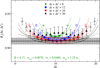
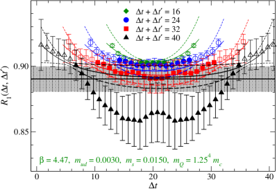
Figure 1: Double ratio (13) to estimate $h_{A_{1}}(1)$ as a function of temporal location of weak currents ${\Delta t}$. The open symbols show all data at different choices of the source-sink separations ${\Delta t}+{\Delta t^{\prime}}$, whereas the filled symbols are data used in the fit (14) to extract the ground state matrix element shown by the horizontal black band. The thick (thin) curves are fit curves inside (outside) the fit range. The left panel shows the data at our smallest pion mass $M_{\pi}\!\simeq 230$ MeV ($a^{-1}\!\simeq\!2.5$ GeV, $m_{Q}\!=\!1.25m_{c}$), whereas the right panel is for our largest cutoff $a^{-1}\!\simeq\!4.5$ GeV ($M_{\pi}\!\simeq\!300$ GeV, $m_{Q}\!=\!1.25^{4}m_{c}$). All data are shifted along the horizontal axis so that the mid-point ${\Delta t}\!=\!{\Delta t^{\prime}}$ is located at the center of the panel (${\Delta t}=10$ and 20 in the left and right panels, respectively). The symbols are further but slightly shifted along the horizontal axis for clarity.

To precisely extract the form factors, we construct ratios of the correlation functions, in which unnecessary overlap factors and exponential damping factors cancel for the ground-state contribution Hashimoto et al. (1999). The statistical fluctuation is also expected to partly cancel in such a ratio. With $B$ and $D^{*}$ mesons at rest, the vector current matrix element (6) vanishes, and the axial vector one (7) is sensitive only to the axial vector form factor $h_{A_{1}}$ at zero recoil, which is the fundamental input to determine $|V_{cb}|$. In order to precisely determine $h_{A_{1}}(1)$, we employ a double ratio

$$R_{1}({\Delta t},{\Delta t^{\prime}}) = \frac{C_{A_{1}}^{BD^{*}}({\Delta t},{\Delta t^{\prime}};{\bf 0},{\bf 0},{\epsilon^{\prime}})\,C_{A_{1}}^{D^{*}B}({\Delta t},{\Delta t^{\prime}};{\bf 0},{\bf 0},{\epsilon^{\prime}})}{C_{V_{4}}^{BB}({\Delta t},{\Delta t^{\prime}};{\bf 0},{\bf 0})\,C_{V_{4}}^{D^{*}D^{*}}({\Delta t},{\Delta t^{\prime}};{\bf 0},{\bf 0},{\epsilon^{\prime}},{\epsilon^{\prime}})}\xrightarrow[{\Delta t},{\Delta t^{\prime}}\to\infty]{}|h_{A_{1}}(1)|^{2},$$ (13)

where the $D^{*}$ polarization is chosen as ${\epsilon^{\prime}}\!=\!(1,0,0,0)$ along the polarization of the current inserted, i.e. $A_{1}$. The left panel of Fig. 1 shows our results for this ratio at our smallest $M_{\pi}$ and $a^{-1}$ with $m_{Q}\!=\!1.25m_{c}$. Note that the ratio is symmetrized as $R_{1}({\Delta t},{\Delta t^{\prime}})\!\to\!\left\{R_{1}({\Delta t},{\Delta t^{\prime}})+R_{1}({\Delta t^{\prime}},{\Delta t})\right\}/2$, since we use the same smearing function for both the source and sink operators. We observe a reasonable consistency among data at intermediate values of the source-sink separation ${\Delta t}+{\Delta t^{\prime}}\!=\!12$ (circles) and 16 (squares). The excited state contribution could potentially be significant but not large ($\lesssim\,1$ %) for the smallest ${\Delta t}+{\Delta t^{\prime}}\!=\!8$ (diamonds). Data at the largest ${\Delta t}+{\Delta t^{\prime}}\!=\!20$ (triangles) show a long plateau and are consistent with those at smaller ${\Delta t}+{\Delta t^{\prime}}$ within the large statistical errors. These observations suggest that the data at ${\Delta t}+{\Delta t^{\prime}}\!=\!12$, which is roughly 1 fm, are dominated by the ground state contribution at least at the midpoint ${\Delta t}\!\sim\!{\Delta t^{\prime}}$. The situation is similar in the right panel of the same figure for our largest $a^{-1}$ and with $m_{Q}\!=\!1.25^{4}m_{c}$, where data around midpoint ${\Delta t}\!\sim\!{\Delta t^{\prime}}$ are consistent among all simulated source-sink separations within 2 $\sigma$.

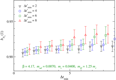
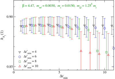
Figure 2: Axial form factor $h_{A_{1}}(1)$ from fit (14) as a function of lower cut ${{\Delta t}_{\rm min}}$. Left and right panels show data at $(a^{-1},M_{\pi})\!\simeq\!(2.5~{}{\rm GeV},230~{}{\rm MeV})$ and $(4.5~{}{\rm GeV},300~{}{\rm MeV})$, respectively. Different symbols show data with different values for ${{\Delta t^{\prime}}_{\rm min}}$. Symbols are slightly shifted along the horizontal axis for clarity.

We find that all data are well described by the following fitting form including effects from the first excited states

$$R_{1}({\Delta t},{\Delta t^{\prime}}) = |h_{A_{1}}(1)|^{2}\left(1+ae^{-\Delta M_{B}{\Delta t}}+be^{-\Delta M_{D^{*}}{\Delta t}}+ae^{-\Delta M_{B}{\Delta t^{\prime}}}+be^{-\Delta M_{D^{*}}{\Delta t^{\prime}}}\right)$$ (14)

with $\chi^{2}/{\rm d.o.f.}\!\lesssim\!1$ for a wide range of the values of ${\Delta t}$ and ${\Delta t^{\prime}}$. Here $\Delta M_{B(D^{*})}$ represents the energy difference between the $B(D^{*})$ meson ground state and the first excited state of the same quantum numbers, and is set to the value estimated from a two-exponential fit to the two-point function $C^{B(D^{*})}({\Delta t};{\bf 0})$. The fit range is chosen such that all the data of $R_{1}({\Delta t},{\Delta t^{\prime}})$ with the source-to-current (current-to-sink) separation ${\Delta t}^{(\prime)}$ equal to or larger than a lower cut ${\Delta t}^{(\prime)}_{\rm min}$ are included irrespective of the source-sink separation ${\Delta t}+{\Delta t^{\prime}}$. As shown in the left panel of Fig. 2, our result for $h_{A_{1}}(1)$ is stable against the choice of the lower cuts ${{\Delta t}_{\rm min}}$ and ${{\Delta t^{\prime}}_{\rm min}}$.

The right panels of Figs. 1 and 2 for our largest $a^{-1}$ also show ground state dominance with ${\Delta t}+{\Delta t^{\prime}}\!\gtrsim\!23a\!\sim\!1$ fm and stability of $h_{A_{1}}(1)$ against the choice of the fit range, respectively. The situation is similar for other simulation parameters.

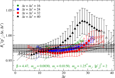
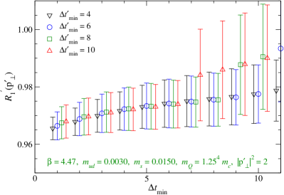
Figure 3: Left: ratio $R_{1}^{\prime}({{\bf p}^{\prime}_{\perp}};{\Delta t},{\Delta t^{\prime}})$ (15) to study $w$-dependence of $h_{A_{1}}$. Right: fitted value of $R_{1}^{\prime}({{\bf p}^{\prime}_{\perp}};{\Delta t},{\Delta t^{\prime}})$ with different choices of the lower cuts ${{\Delta t}_{\rm min}}$ and ${{\Delta t^{\prime}}_{\rm min}}$. Both panels show data at $a^{-1}\!\simeq\!4.5$ GeV and $M_{\pi}\!\simeq\!300$ MeV with the $D^{*}$ momentum $|{{\bf p}_{\perp}}|=\sqrt{2}$.

In order to extract form factors at non-zero recoils, the $D^{*}$ momentum and polarization vector need to be chosen appropriately. The axial vector matrix element (7) is sensitive only to $h_{A_{1}}$ with a polarization vector ${\boldsymbol{\epsilon}}^{\prime}\!=\!(1,0,0)$ and a momentum ${{\bf p}^{\prime}_{\perp}}$ that satisfies ${\epsilon^{\prime*}}p^{\prime}_{\perp}\!=\!0$ as well as ${\epsilon^{\prime*}}v\!=\!0$. Then, the recoil parameter dependence of $h_{A_{1}}$ may be studied from the following ratio

$$R_{1}^{\prime}({{\bf p}^{\prime}_{\perp}};{\Delta t},{\Delta t^{\prime}})=\frac{C_{A_{1}}^{BD^{*}}({\Delta t},{\Delta t^{\prime}};{\bf 0},{{\bf p}^{\prime}_{\perp}},{\epsilon^{\prime}})\,C^{D^{*}}_{sl}({\Delta t^{\prime}};{\bf 0},{\epsilon^{\prime}})}{C_{A_{1}}^{BD^{*}}({\Delta t},{\Delta t^{\prime}};{\bf 0},{\bf 0},{\epsilon^{\prime}})\,C^{D^{*}}_{sl}({\Delta t^{\prime}},{{\bf p}^{\prime}_{\perp}},{\epsilon^{\prime}})}\xrightarrow[{\Delta t},{\Delta t^{\prime}}\to\infty]{}\frac{w+1}{2}\frac{h_{A_{1}}(w)}{h_{A_{1}}(1)}.$$ (15)

Here we use the two-point function with the local sink $C^{D^{*}}_{\rm sl}$ (12) as in our study of the $K\!\to\!\pi\ell{\nu_{\ell}}$ decay Aoki et al. (2017). The vector form factor $h_{V}$ can be extracted from the following ratio through the vector current matrix element (6)

$$R_{V}({{\bf p}^{\prime\prime}_{\perp}},{{\bf p}^{\prime}_{\perp}};{\Delta t},{\Delta t^{\prime}}) = \frac{C_{V_{1}}^{BD^{*}}({\Delta t},{\Delta t^{\prime}};{\bf 0},{{\bf p}^{\prime\prime}_{\perp}},{\epsilon^{\prime\prime}})}{C_{A_{1}}^{BD^{*}}({\Delta t},{\Delta t^{\prime}};{\bf 0},{{\bf p}^{\prime}_{\perp}},{\epsilon^{\prime}})}\xrightarrow[{\Delta t},{\Delta t^{\prime}}\to\infty]{}\frac{i\varepsilon_{1ij}\epsilon^{\prime\prime*}_{i}v_{\perp j}^{\prime\prime}}{w+1}\frac{h_{V}(w)}{h_{A_{1}}(w)}.$$ (16)

Here we use two different polarization vectors, ${\boldsymbol{\epsilon}}^{\prime}\!=\!(1,0,0)$ and ${\boldsymbol{\epsilon}}^{\prime\prime}\!=\!(0,1,0)$, and momenta ${\bf p}^{\prime}_{\perp}$ and ${\bf p}^{\prime\prime}_{\perp}$ that satisfy ${\bf p}^{\prime(\prime\prime)}_{\perp}\!\perp\!{\boldsymbol{\epsilon}}^{\prime(\prime\prime)}$. Note that $|{{\bf p}^{\prime\prime}_{\perp}}|\!=\!|{{\bf p}^{\prime}_{\perp}}|$ to share the same recoil parameter $w$, and $v_{\perp j}^{\prime\prime}\!=\!p_{\perp j}^{\prime\prime}/M_{D^{*}}$. We emphasize that renormalization factors of the weak vector and axial currents cancel thanks to chiral symmetry preserved in our simulations.

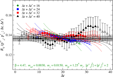
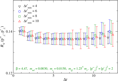
Figure 4: Same as Fig. 3 but for ratio $R_{V}({{\bf p}^{\prime\prime}_{\perp}},{{\bf p}^{\prime}_{\perp}};{\Delta t},{\Delta t^{\prime}})$ (16) to study $h_{V}(w)$.

Figures 3 and 4 show an example of our results for $R_{1}^{\prime}$ and $R_{V}$ at our largest cutoff $a^{-1}\!\simeq\!4.5$ GeV and $m_{Q}\!=\!1.25^{4}m_{c}$. Around the mid-point ${\Delta t}\!\sim\!{\Delta t^{\prime}}$, we observe good consistency in these ratios among all simulated values of the source-sink separation ${\Delta t}+{\Delta t^{\prime}}\!\gtrsim\!1$ fm. A similar ground state dominance is also observed at other simulation points. We carry out a simultaneous fit using a fitting form that takes account of the first excited state contribution as

$$R_{1}^{\prime}({{\bf p}^{\prime}_{\perp}};{\Delta t},{\Delta t^{\prime}}) = R_{1}^{\prime}({{\bf p}^{\prime}_{\perp}})\left(1+ae^{-\Delta M_{B}{\Delta t}}+be^{-\Delta M_{D^{*}}{\Delta t^{\prime}}}\right)$$ (17)

to extract the form factor ratio $h_{A_{1}}(w)/h_{A_{1}}(1)$ from the ground state contribution $R_{1}^{\prime}({{\bf p}^{\prime}_{\perp}})$, and a similar form for $R_{V}({{\bf p}^{\prime\prime}_{\perp}},{{\bf p}^{\prime}_{\perp}};{\Delta t},{\Delta t^{\prime}})$ to extract $h_{V}(w)/h_{A_{1}}(w)$. Our data are well described by this fitting form with $\chi^{2}/{\rm d.o.f.}\!\lesssim\!1$. From these form factor ratios and $h_{A_{1}}(1)$ from $R_{1}$, we calculate $h_{A_{1}}(w)$ and $h_{V}(w)$ at simulated values of $w$.

The axial vector form factors $h_{A_{2}}$ and $h_{A_{3}}$ can be extracted from the axial vector matrix element (7) with the $D^{*}$ spatial momentum ${{\bf p}^{\prime}_{\not\perp}}$ not perpendicular to the spatial polarization vector. The matrix element of $A_{1}$, for instance, has non-zero sensitivity to $h_{A_{1}}$ and $h_{A_{3}}$. We use the following ratio to extract $h_{A_{3}}$

$$R_{3}({{\bf p}^{\prime}_{\not\perp}},{{\bf p}^{\prime}_{\perp}};{\Delta t},{\Delta t^{\prime}}) = r_{Z}\frac{C_{A_{1}}^{BD^{*}}({\Delta t},{\Delta t^{\prime}};{\bf 0},{{\bf p}^{\prime}_{\not\perp}},{\epsilon^{\prime\prime}})}{C_{A_{1}}^{BD^{*}}({\Delta t},{\Delta t^{\prime}};{\bf 0},{{\bf p}^{\prime}_{\perp}},{\epsilon^{\prime}})}$$ (18)

$$\xrightarrow[{\Delta t},{\Delta t^{\prime}}\to\infty]{} {\epsilon^{\prime\prime}}^{*}_{1}-\frac{{\epsilon^{\prime\prime}}^{*}_{4}{v^{\prime}}_{\not\perp,1}}{w+1}\frac{h_{A_{3}}(w)}{h_{A_{1}}(w)},$$

where ${\boldsymbol{\epsilon}}^{\prime}\!=\!(1,0,0)$, ${\boldsymbol{\epsilon}}^{\prime*}{{\bf p}^{\prime}_{\perp}}\!=0$, ${\boldsymbol{\epsilon}}^{\prime\prime*}{{\bf p}^{\prime}_{\not\perp}}\!\neq\!0$, and $|{{\bf p}^{\prime}_{\not\perp}}|\!=\!|{{\bf p}^{\prime}_{\perp}}|$. The factor $r_{Z}\!=\!Z_{D^{*}}({{\bf p}^{\prime}_{\perp}},{\epsilon^{\prime}})/Z_{D^{*}}({{\bf p}^{\prime}_{\not\perp}},{\epsilon^{\prime\prime}})$ appears, since the overlap factor of $D^{*}$ depends on whether the polarization vector is perpendicular to the momentum, even if $|{{\bf p}^{\prime}_{\not\perp}}|\!=\!|{{\bf p}^{\prime}_{\perp}}|$. We estimate as $r_{Z}\!=\!\sqrt{C^{D^{*}}({\Delta t}_{\rm ref},{{\bf p}^{\prime}_{\perp}},{\epsilon^{\prime}})/C^{D^{*}}({\Delta t}_{\rm ref},{{\bf p}^{\prime}_{\not\perp}},{\epsilon^{\prime\prime}})}$ with a reference temporal separation ${\Delta t}_{\rm ref}\!\sim\!T/4$ chosen by inspecting the statistical accuracy and the ground state saturation of $r_{Z}$. A similar ratio but with $A_{4}$ in the numerator is also sensitive to $h_{A_{2}}$

$$R_{2}({{\bf p}^{\prime}_{\not\perp}},{{\bf p}^{\prime}_{\perp}};{\Delta t},{\Delta t^{\prime}}) = r_{Z}\frac{C_{A_{4}}^{BD^{*}}({\Delta t},{\Delta t^{\prime}};{\bf 0},{{\bf p}^{\prime}_{\not\perp}},{\epsilon^{\prime\prime}})}{C_{A_{1}}^{BD^{*}}({\Delta t},{\Delta t^{\prime}};{\bf 0},{{\bf p}^{\prime}_{\perp}},{\epsilon^{\prime}})}$$ (19)

$$\xrightarrow[{\Delta t},{\Delta t^{\prime}}\to\infty]{} {\epsilon^{\prime\prime}}^{*}_{4}\left[1-\frac{1}{w+1}\left\{\frac{h_{A_{2}}(w)}{h_{A_{1}}(w)}+v_{\not\perp,4}\frac{h_{A_{3}}(w)}{h_{A_{1}}(w)}\right\}\right].$$

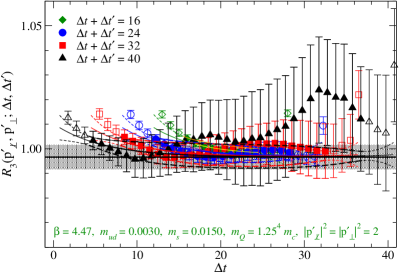
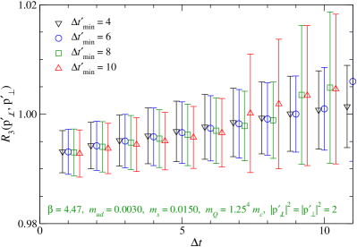
Figure 5: Same as Fig. 3 but for ratio $R_{3}({{\bf p}_{\not\perp}},{{\bf p}_{\perp}};{\Delta t},{\Delta t^{\prime}})$ (18) to study $h_{A_{3}}(w)$.

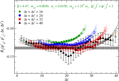
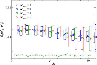
Figure 6: Same as Fig. 3 but for ratio $R_{2}({{\bf p}_{\not\perp}},{{\bf p}_{\perp}};{\Delta t},{\Delta t^{\prime}})$ (18) to study $h_{A_{2}}(w)$.

We plot our results for $R_{3}$ and $R_{2}$ on our finest lattice in Figs. 5 and 6, respectively. Similar to other ratios, the excited state contamination is not large. The fit similar to (17) yields the ground state contributions, $R_{3}({{\bf p}^{\prime}_{\not\perp}},{{\bf p}^{\prime}_{\perp}})$ and $R_{2}({{\bf p}^{\prime}_{\not\perp}},{{\bf p}^{\prime}_{\perp}})$, which are stable against the choice of the fit range: we do not observe ${\Delta t}^{(\prime)}_{\rm min}$ dependence beyond 1 $\sigma$ level when ${{\Delta t}_{\rm min}}+{{\Delta t^{\prime}}_{\rm min}}\!\lesssim\!16$, that is our smallest value of the source-sink separation ${\Delta t}+{\Delta t^{\prime}}$. The error rapidly increases at larger values of ${\Delta t}^{(\prime)}_{\rm min}$, because less data are available for the fit. From $R_{2}$, $R_{3}$ and $h_{A_{1}}$ extracted above, we can calculate $h_{A_{2}}$ and $h_{A_{3}}$.

For one of the $D^{*}$ momenta ${{\bf p}^{\prime}}\!=\!(1,1,1)$, it is not straightforward to use the above-mentioned correlator ratios, which use $C_{A_{1}}^{BD^{*}}({\Delta t},{\Delta t^{\prime}};{\bf 0},{{\bf p}^{\prime}},{\epsilon^{\prime}})$ with ${\boldsymbol{\epsilon}}^{\prime*}{{{\bf p}^{\prime}}}\!=\!0$ as a correlator sensitive only to $h_{A_{1}}(w)$. In this case, we use a linear combination

$$C_{A_{1}}^{BD^{*}}({\Delta t},{\Delta t^{\prime}};{\bf 0},{{\bf p}^{\prime}},{\epsilon^{\prime}})-C_{A_{1}}^{BD^{*}}({\Delta t},{\Delta t^{\prime}};{\bf 0},{{\bf p}^{\prime}},{\epsilon^{\prime\prime}}) \propto (w+1)h_{A_{1}}(w)$$ (20)

which only involves $h_{A_{1}}$ with ${\boldsymbol{\epsilon}}^{\prime}\!=\!(1,0,0)$ and ${\boldsymbol{\epsilon}}^{\prime\prime}\!=\!(0,1,0)$.

The double ratio $R_{1}$ enables us to calculate $h_{A_{1}}(1)$ with 1 % statistical error or better, as it only involves correlators with zero momentum and the statistical fluctuation partially cancels between the numerator and denominator. At non-zero recoil, the numerator of $R_{1}^{\prime}$ ($R_{V}$) is exclusively sensitive to $h_{A_{1}}$ ($h_{V}$), and the statistical error of $h_{A_{1}}$ and $h_{V}$ is typically a few %. This is not the case for $h_{A_{2}}$ and $h_{A_{3}}$ with our set up where the $B$ meson is at rest. The numerator of $R_{3}$ involves $h_{A_{1}}$ and $h_{A_{3}}$, and the typical precision for $h_{A_{3}}$ is 10 – 20 %. The statistical error increases to $\gtrsim\!40$ % for $h_{A_{2}}$, since the central value is suppressed by heavy quark symmetry and $R_{2}$ is a linear combination of all axial form factors.

We note that, thanks to chiral symmetry, finite renormalization factors for the weak vector and axial currents cancel in the above correlator ratios (13), (15), (16), (18) and (19). While discretization effects to the wave function renormalization are not small Fahy et al. (2016), these also cancel in the ratios.

III Extrapolation to continuum limit and physical quark masses

III.1 Choice of fitting form

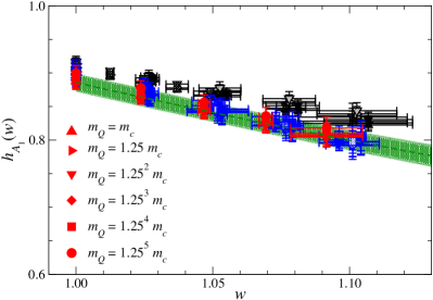
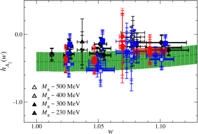
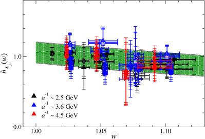
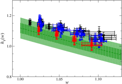
Figure 7: Form factors as a function of recoil parameter $w$. The top-left, top-right, bottom-left and bottom-right panels show results for $h_{A_{1}}$, $h_{A_{2}}$, $h_{A_{3}}$ and $h_{V}$, respectively. The black, blue and red symbols show data at $a^{-1}\!\sim\!2.5$, 3.6 and 4.5 GeV, whereas the open, pale-shaded, filled and dark-shaded ones are at $M_{\pi}\!\sim\!500$, 400, 300 and 230 MeV, respectively. Symbols with different shapes are obtained with different bottom quark masses. (See the legend in the plots.) The green bands show the form factors extrapolated to the continuum limit and physical quark masses. The pale and dark shaded bands represent their statistical and total uncertainties, respectively.

Our results for the form factors obtained at various simulation parameters are plotted as a function of the recoil parameter $w$ in Fig. 7. We find that the results with different heavy and light quark masses are all close to each other. It also turns out that the discretization effects are not large.

We extrapolate these results to the continuum limit and physical quark masses based on next-to-leading order heavy meson chiral perturbation theory (NLO HMChPT) Randall and Wise (1993); Savage (2002). The extrapolation form is generically written as

$$h_{X}/\eta_{X} = c+\frac{{g_{D^{*}D\pi}}^{2}}{2\Lambda_{\chi}^{2}}\bar{F}_{\rm log}\!\left({\xi_{\pi}},\Delta_{D},\Lambda_{\chi}\right)+c_{\pi}{\xi_{\pi}}+c_{\eta_{s}}{\xi_{\eta_{s}}}+c_{Q}{\epsilon_{Q}}$$ (21)

$$+c_{a}{\xi_{a}}+c_{am_{Q}}{\xi_{am_{Q}}}+c_{w}(w-1)+d_{w}(w-1)^{2}\hskip 14.22636pt(X\!=\!A_{1},A_{2},A_{3}{\rm\ and\ }V),\hskip 14.22636pt$$

which comprises the constant term, chiral logarithm at $w\!=\!1$ and leading corrections in small expansion parameters

$${\xi_{\pi}}=\frac{M_{\pi}^{2}}{\Lambda_{\chi}^{2}},\hskip 5.69054pt{\xi_{\eta_{s}}}=\frac{M_{\eta_{s}}^{2}}{\Lambda_{\chi}^{2}},\hskip 5.69054pt{\epsilon_{Q}}=\frac{\bar{\Lambda}}{2m_{Q}},\hskip 5.69054pt{\xi_{a}}=(\Lambda a)^{2},\hskip 5.69054pt{\xi_{am_{Q}}}=(am_{Q})^{2},$$ (22)

with $M_{\eta_{s}}^{2}\!=\!2M_{K}^{2}-M_{\pi}^{2}$, $\Lambda_{\chi}\!=\!4\pi f_{\pi}$, and nominal values of $\bar{\Lambda}\!=\!\Lambda\!=\!500$ MeV.

We denote the one-loop integral function for the chiral logarithm by $\bar{F}_{\rm log}\!\left({\xi_{\pi}},\Delta_{D},\Lambda_{\chi}\right)$, where $\Delta_{D}\!=\!M_{D^{*}}-M_{D}$ is the $D^{*}$-$D$ mass splitting. While the loop function can be approximated as $\bar{F}_{\rm log}\!\left({\xi_{\pi}},\Delta_{D},\Lambda_{\chi}\right)\!=\!\Delta_{D}^{2}\ln[{\xi_{\pi}}]+O(\Delta_{D}^{3})$, we use its explicit form in Ref. Savage (2002). For the $D^{*}D\pi$ coupling, we take a value of ${g_{D^{*}D\pi}}\!=\!0.53(8)$, which was employed in the Fermilab/MILC paper Bailey et al. (2014) and covers previous lattice estimates Detmold et al. (2012); Becirevic and Sanfilippo (2013); Can et al. (2013); Bernardoni et al. (2015); Flynn et al. (2016). This choice does not lead to a large systematic uncertainty, because the chiral logarithm is suppressed by the small mass splitting squared $\Delta_{D}^{2}$.

The so-called $\xi$ expansion in ${\xi_{\pi}}$ and ${\xi_{\eta_{s}}}$ is employed for the chiral expansion: namely, we use the measured meson masses squared, $M_{\pi}^{2}$ and $M_{\eta_{s}}^{2}$, instead of quark masses $m_{ud}$ and $m_{s}$, respectively, as well as quark-mass dependent $f_{\pi}$ for $\Lambda_{\chi}$ instead of the decay constant $f$ in the chiral limit. This is motivated by our observation Noaki et al. (2008) that the $\xi$-expansion shows better convergence of the chiral expansion for light meson observables compared to the $x$-expansion with $x\!=\!2Bm_{q}/(4\pi f)^{2}$, where $B$ gives the lowest order relation $M_{\pi}^{2}\!=\!2Bm_{ud}$.

The extrapolation form explicitly includes the one-loop radiative correction $\eta_{X}$ for the matching of the heavy-heavy currents between QCD and HQET Falk et al. (1990); Falk and Grinstein (1990); Neubert (1992). Remaining heavy quark mass dependence is then parametrized by polynomials of ${\epsilon_{Q}}\!\propto\!1/m_{Q}$. The $m_{Q}$ dependence of the form factors is mild as shown in Fig. 7, and is well described by the linear term $c_{Q}{\epsilon_{Q}}$ in Eq. (21). For $h_{A_{1}}$, however, it is modified as $c_{Q}(w-1){\epsilon_{Q}}$ to be consistent with Luke’s theorem Luke (1990), and we add the quadratic term $d_{Q}{\epsilon_{Q}}^{2}$ to take account of possible $m_{Q}$ dependence at $w\!=\!1$.

The discretization effects in the form factors also turn out to be mild with our choice of parameters, $a^{-1}\!\gtrsim\!2.5$ GeV and $m_{Q}\!\leq 0.7a^{-1}$. These are described by an expansion, i.e. linear in the $m_{Q}$ independent and dependent parameters ${\xi_{a}}$ and ${\xi_{am_{Q}}}$, respectively.

In this study, we first extrapolate the form factors to the continuum limit and physical quark masses, and then parametrize the $w$ dependence by using the model independent BGL parametrization, because it may not be simply combined with the chiral and heavy quark expansions. Concerning the $w$ dependence, therefore, the fit form (21) with an expansion in $w-1$ is used to interpolate our results. Figure 7 shows that our data do not show strong curvature in the simulation region of $1\!\leq\!w\!\lesssim\!1.1$, and can be well described with only up to the quadratic term.

Table 3: Fit parameters from continuum and chiral extrapolation of form factors (21).

. $h_{X}$ $\chi^{2}$/d.o.f $c$ $c_{\pi}$ $c_{\eta_{s}}$ $c_{Q}$ $d_{Q}$ $c_{a}$ $c_{am_{Q}}$ $c_{w}$ $d_{w}$ $h_{A_{1}}$ 0.14(11) 0.898(54) 0.68(19) 0.08(16) -0.18(32) 0.59(17) 0.37(26) 0.0376(89) -0.953(70) 0.67(22) $h_{A_{2}}$ 0.18(13) -0.5(1.0) 0.9(3.6) -0.0(2.6) 0.13(49) – 3.3(3.0) -0.022(67) -0.41(86) 10.3(7.1) $h_{A_{3}}$ 0.18(13) 0.91(90) -0.4(3.3) 0.3(2.4) 1.25(47) – -3.4(2.7) 0.117(62) -1.72(75) 1.9(6.1) $h_{V}$ 0.15(14) 0.87(13) 1.47(45) 0.39(37) 0.33(13) – -0.51(63) 0.092(18) -1.32(14) 0.6(1.3)

Numerical results of our continuum and chiral extrapolation are summarized in Table 3. The polynomial coefficients turn out to be $O(1)$ or less with our choice of the dimensionless expansion parameters (22), which are normalized by appropriate scales. Many of them are consistent with zero reflecting the mild dependence on the lattice spacing and quark masses mentioned above. As a result, our results for the form factors are well described by the fitting form (21) with $\chi^{2}/{\rm d.o.f.}\!\lesssim\!0.2$.

III.2 Systematic uncertainties

III.2.1 Correlated fit

With limited statistics, the covariance matrix $C$ of our form factor data has exceptionally small eigenvalues with large statistical error. In this study, we test two methods to take the correlation into account in the combined continuum and chiral extrapolation. First, as in the study of $B\!\to\!\pi\ell{\nu_{\ell}}$ Colquhoun et al. (2022), we introduce a lower cut of the eigenvalue (singular value) $\lambda_{\rm cut}$. Effects of the exceptionally small eigenvalues are suppressed by replacing eigenvalues smaller than $\lambda_{\rm cut}$ by $\lambda_{\rm cut}$ in the singular value decomposition of $C$ as

$$C \sim \sum_{k\leq n_{\rm cut}}\lambda_{\rm cut}\,u_{k}u_{k}^{T}+\sum_{k>n_{\rm cut}}\lambda_{k}u_{k}u_{k}^{T},$$ (23)

where $u_{k}$ represents the eigenvector corresponding to the eigenvalue $\lambda_{k}$. Here eigenvalues are sorted in ascending order ($\lambda_{k}\!<\!\lambda_{k+1}$) and $n_{\rm cut}$ satisfies $\lambda_{n_{\rm cut}}\!<\!\lambda_{\rm cut}\!<\!\lambda_{n_{\rm cut}+1}$. We choose $\lambda_{\rm cut}$ such that all eigenvalues below $\lambda_{\rm cut}$ have statistical error larger than 100 %. The second method is the so-called shrinkage estimate of the covariance matrix Stein (1956); Ledoit and Wolf (2004), which amounts to replacing $C_{ij}$ by

$$\rho\delta_{ij}C_{ii}+(1-\rho)C_{ij}.$$ (24)

With $0\!\leq\!\rho\!\leq\!1$, the shrinkage is an interpolation between the uncorrelated ($\rho\!=\!1$) and correlated ($\rho\!=\!0$) fits. An optimal value of $\rho$ can be estimated by minimizing a loss function Ledoit and Wolf (2004). We observed, however, that results of the continuum and chiral extrapolation do not strongly depend on the choice of $\lambda_{\rm cut}$ and $\rho$. In this study, we therefore employ the singular value cut for our main results, since this is a conservative approach, which only tends to increase the final error. The shift of the fit results obtained with the shrinkage estimator is treated as a systematic error due to the estimate of $C$.

III.2.2 Fitting form

The highest order is quadratic in the recoil parameter $w-1$ expansion and heavy quark expansion for $h_{A_{1}}$, and linear for other expansions including chiral and finite $a$ expansions. The systematic error due to this choice is estimated by repeating the continuum and chiral extrapolation without one of the highest order terms, if the corresponding coefficient is poorly determined, otherwise by adding a yet higher order term.

Possible higher order corrections in the chiral expansion are also examined by testing the $x$-expansion. We also test a multiplicative form

$$h_{X}/\eta_{X} = c+\left(1+\frac{{g_{D^{*}D\pi}}^{2}}{2\Lambda_{\chi}^{2}}\bar{F}_{\rm log}\!\left({\xi_{\pi}},\Delta_{D},\Lambda_{\chi}\right)+c_{\pi}{\xi_{\pi}}+c_{\eta_{s}}{\xi_{\eta_{s}}}\right)\left(1+c_{Q}{\epsilon_{Q}}\right)$$ (25)

$$\times\left(1+c_{a}{\xi_{a}}+c_{am_{Q}}{\xi_{am_{Q}}}\right)\left\{1+c_{w}(w-1)+d_{w}(w-1)^{2}\right\}\hskip 14.22636pt$$

to examine the potential effect of cross terms. We find that these alternative fits yield a change of the fit results well below the statistical error.

III.2.3 Inputs

The lattice cutoff $a^{-1}$, physical meson masses $M_{\pi}$, $M_{K}$, $M_{\eta_{b}}$, and the $D^{*}D\pi$ coupling ${g_{D^{*}D\pi}}$ are inputs to the continuum and chiral extrapolation. Since the masses have been measured very precisely, we take account of the uncertainty due to $a^{-1}$ and ${g_{D^{*}D\pi}}$ by repeating the extrapolation with each input shifted by $\pm$ 1 $\sigma$.

We set $M_{\pi}$ and $M_{K}$ to those in the isospin limit as in our determination of $a$ Colquhoun et al. (2022). To examine the isospin breaking effects to the form factors, we test the continuum and chiral extrapolation to $M_{\pi}\!=\!M_{\pi^{0}}$ and $M_{\pi^{\pm}}$ as well as $M_{K}\!=\!M_{K^{0}}$ and $M_{K^{\pm}}$. We also test the heavy quark expansion parameter replaced with ${\epsilon_{Q}}\!=\!\bar{\Lambda}/2M_{B}$ and compare the extrapolations using $M_{B}=M_{B^{0}}$ and $M_{B^{\pm}}$. The difference in the form factor can be considered as an estimate of the strong isospin breaking effect. It turns out to be small as suggested by the mild quark mass dependence of the form factors. We include this in the systematic uncertainty so that our synthetic data for the form factors can be used for both the neutral and charged $B$ meson decays.

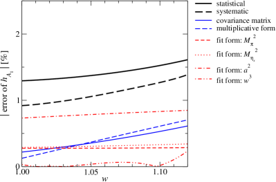
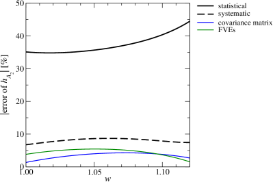
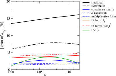
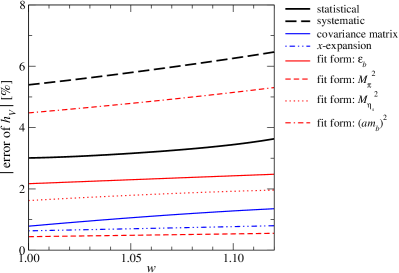
Figure 8: Uncertainties of form factors as a function of $w$. The top-left, top-right, bottom-left and bottom-right panels show uncertainties of $h_{A_{1}}$, $h_{A_{2}}$, $h_{A_{3}}$ and $h_{V}$, respectively. The thick solid and dashed lines show the statistical and total systematic uncertainties, while the thin lines show a breakdown of the latter. Just for clarity, we omit small systematic errors below 0.2 % ($h_{A_{1}}$), 4 % ($h_{A_{2}}$), 1 % ($h_{A_{3}}$) and 0.5 % ($h_{V}$) in the whole simulated region of $w$.

III.2.4 Finite volume effects (FVEs)

Our spatial lattice size satisfies $M_{\pi}L\!\geq\!4$. At our smallest pion mass on the coarsest lattice, we also simulate a smaller size $L\!\simeq\!3.0M_{\pi}^{-1}$ to directly examine FVEs. Comparison between the two volumes at that simulation point does not show any significant deviation: for instance, $h_{A_{1}}$ at $w\!=\!1$ is consistent within statistical error of $\lesssim\,1$ %. We also repeat the continuum and chiral extrapolation by replacing the form factors at the smallest $M_{\pi}$ with those on the smaller $L$. The change in the fit results is included in the systematic uncertainty, but turns out to be well below the statistical uncertainty. We conclude that finite volume effects are not significant in our simulation region of $M_{\pi}\!\gtrsim\!230$ MeV.

III.2.5 Accuracy of continuum and chiral extrapolation

Figure 8 shows the estimate of various uncertainties for the form factors in the continuum limit and at the physical quark masses as a function of $w$. As discussed in Sec. II, the axial (vector) matrix element is exclusively sensitive to $h_{A_{1}}(w)$ ($h_{V}(w)$) with an appropriate choice of the $D^{*}$ meson polarization vector and momentum. Combined with a precise determination at zero-recoil, the total uncertainty of $h_{A_{1}}$ is about 2 % in our simulation region of $w$, and the largest uncertainty comes from statistics and discretization effects. On the other hand, either $D^{*}$ or $B$ needs to have non-zero momentum to determine $h_{V}$, which is, therefore, less accurate. The total accuracy is $\lesssim\!7$ % with 3 –4 % statistical and $\sim\!5$ % discretization errors.

Since the simulated bottom quark masses are not far below the lattice cut-off ($m_{b}\!\leq\!0.7a^{-1}$), we repeat the continuum and chiral extrapolation only using the data with $m_{b}\!\leq\!0.5\,a^{-1}$. The change in the fit results is well below the statistical uncertainty. We therefore conclude that our continuum extrapolation in the relativistic approach is controlled.

On the other hand, the axial form factors, $h_{A_{2}}$ and $h_{A_{3}}$, have larger uncertainty, i.e. 40 % and 15 %, respectively, dominated by the statistical error. Towards a more precise determination, it would be advantageous to simulate moving $B$ mesons so as to have matrix elements more sensitive to these form factors.

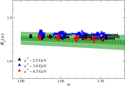
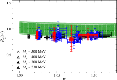
Figure 9: Form factor ratios $R_{1}(w)$ (left panel) and $R_{2}(w)$ (right panel) as a function of recoil parameter $w$. Results at simulated parameters are plotted in symbols, which have the same meaning as in Fig. 7. The green bands show these ratios in the continuum limit and at physical quark masses reproduced by the continuum and chiral extrapolation of form factors (21).

Previous determinations of ${|V_{cb}|}$ often employed a HQET-based parametrization by Caprini, Lellouch and Neubert of $h_{A_{1}}$ and form factor ratios

$$R_{1}(w)\!=\!\frac{h_{V}(w)}{h_{A_{1}}(w)},\hskip 14.22636ptR_{2}(w)\!=\!\frac{rh_{A_{2}}(w)+h_{A_{3}}(w)}{h_{A_{1}}(w)},$$ (26)

where higher order HQET corrections are expected to be partially canceled Caprini et al. (1998). Figure 9 shows that these ratios also have mild parameter dependences and can be safely extrapolated to the continuum limit and physical quark masses. We, however, do not employ the model-dependent CLN parametrization in the following analysis.

IV Form factors as a function of the recoil-parameter

IV.1 Fit to lattice data

From the continuum and chiral extrapolation in the previous section, we generate synthetic data of the form factors in the relativistic convention,

$$\langle D^{*}({\epsilon^{\prime}},{p^{\prime}})|V_{\mu}|B(p)\rangle = i\varepsilon_{\mu\nu\rho\sigma}\,{\epsilon^{\prime*}}^{\nu}p^{\prime\rho}p^{\sigma}\,g(w),$$ (27)

$$\langle D^{*}({\epsilon^{\prime}},{p^{\prime}})|A_{\mu}|B(p)\rangle = \epsilon_{\mu}^{\prime*}\,f(w)-({\epsilon^{\prime*}}p)\left\{(p+{p^{\prime}})_{\mu}\,a_{+}(w)+(p-{p^{\prime}})_{\mu}\,a_{-}(w)\right\},\hskip 28.45274pt$$ (28)

with which the BGL parametrization was originally proposed. A kinematic invariant $k\!=\!\sqrt{\left(t_{+}-q^{2}\right)\left(t_{-}-q^{2}\right)/4t}$ is defined with the maximum value of the momentum transfer $q^{2}_{\rm max}\!=\!t_{-}\!=\!\left(M_{B}-M_{D^{*}}\right)^{2}$, which corresponds to the zero recoil limit, and the threshold $t_{+}\!=\!\left(M_{B}+M_{D^{*}}\right)^{2}$ for the $W\!\to\!BD^{*}$ production channel. Instead of $a_{+}$ and $a_{-}$, it is common to use linear combinations

$${{\mathcal{F}}_{1}}(w) = \frac{1}{M_{D^{*}}}\left\{\frac{1}{2}\left(M_{B}^{2}-M_{D^{*}}^{2}-q^{2}\right)f(w)+2k^{2}q^{2}a_{+}(w)\right\},$$ (29)

$${{\mathcal{F}}_{2}}(w) = \frac{1}{M_{D^{*}}}\left\{f(w)+\left(M_{B}^{2}-M_{D^{*}}^{2}\right)a_{+}(w)+q^{2}a_{-}(w)\right\}.$$ (30)

These are related to the form factors in the HQET convention as

$$g(w) = \frac{1}{M_{B}\sqrt{r}}h_{V}(w),$$ (31)

$$f(w) = M_{B}\sqrt{r}(w+1)h_{A_{1}}(w),$$ (32)

$${{\mathcal{F}}_{1}}(w) = M_{B}^{2}\sqrt{r}(w+1)\left[(w-r)h_{A_{1}}(w)-(w-1)\left\{rh_{A_{2}}(w)+h_{A_{3}}(w)\right\}\right],$$ (33)

$${{\mathcal{F}}_{2}}(w) = \frac{1}{\sqrt{r}}\left\{(w+1)h_{A_{1}}(w)+(rw-1)h_{A_{2}}(w)+(r-w)h_{A_{3}}\right\}.$$ (34)

We note that there are two kinematical constraints to be satisfied at the minimum ($w\!=\!1$) and maximum values of $w$ (${w_{\rm max}}\!=\!(1+r^{2})/2r$ with $m_{\ell}\!=\!0$)

$${{\mathcal{F}}_{1}}(1) = M_{B}(1-r)f(1),$$ (35)

$${{\mathcal{F}}_{2}}({w_{\rm max}}) = \frac{1+r}{M_{B}^{2}r(1-r)({w_{\rm max}}+1)}{{\mathcal{F}}_{1}}({w_{\rm max}}).$$ (36)

With these form factors, we can write the helicity amplitudes for a given helicity of the intermediate $W$ boson, and the differential decay rate with respect to $w$ in simple forms

$$H_{\pm}(w) = f(w)\mp M_{B}^{2}r\sqrt{w^{2}-1}g(w),$$ (37)

$$H_{0}(w) = \frac{1}{\sqrt{q^{2}}}{{\mathcal{F}}_{1}}(w),$$ (38)

$$H_{S}(w) = M_{B}r\sqrt{\frac{w^{2}-1}{1-2rw+r^{2}}}{{\mathcal{F}}_{2}}(w),$$ (39)

and

$$\frac{d\Gamma}{dw} = \frac{G_{F}^{2}}{16\pi^{3}}|V_{cb}|^{2}|\eta_{EW}|^{2}M_{B}r^{2}\sqrt{w^{2}-1}\left(1-\frac{m_{\ell}^{2}}{q^{2}}\right)^{2}$$ (40)

$$\hskip 14.22636pt\times\left[\frac{q^{2}}{3}\left(1+\frac{m_{\ell}^{2}}{2q^{2}}\right)\left\{|H_{+}(w)|^{2}+|H_{-}(w)|^{2}+|H_{0}(w)|^{2}\right\}+\frac{m_{\ell}^{2}}{2}|H_{S}(w)|^{2}\right].\hskip 28.45274pt$$

From the continuum and chiral extrapolation presented in Sec. III, synthetic data of $f$, $g$ and ${{\mathcal{F}}_{1,2}}$ are calculated at reference values of the recoil parameter ${w_{\rm ref}}$ through the relations (31) – (34). We take ${w_{\rm ref}}\!=\!1.025$, 1.060 and 1.100, which spans the whole simulated region of $w$, since our continuum and chiral extrapolation interpolates $h_{A_{\{1,2,3\}}}$ and $h_{V}$ in $w$. Three values are chosen, because the interpolation involves three fit parameters. The numerical values together with their covariance matrix are presented in Table 4.

Table 4: Synthetic data of form factors $f$, ${{\mathcal{F}}_{1,2}}$ and $g$ in the relativistic convention. The central value and total error are in the second column, and the correlation matrix is in the third to fourteenth columns.

. $f(1.025)$ $f(1.060)$ $f(1.100)$ ${{\mathcal{F}}_{1}}(1.025)$ ${{\mathcal{F}}_{1}}(1.060)$ ${{\mathcal{F}}_{1}}(1.100)$ ${{\mathcal{F}}_{2}}(1.025)$ ${{\mathcal{F}}_{2}}(1.060)$ ${{\mathcal{F}}_{2}}(1.100)$ $g(1.025)$ $g(1.060)$ $g(1.100)$ $f(1.025)$ 5.6928(936) 1.00000 0.98385 0.93944 0.94354 0.71378 0.49823 0.24518 0.22123 0.21755 0.22911 0.22641 0.22699 $f(1.060)$ 5.5879(992) 0.98385 1.00000 0.98338 0.92328 0.70780 0.49984 0.22221 0.20401 0.20620 0.22112 0.22194 0.22694 $f(1.100)$ 5.473(109) 0.93944 0.98338 1.00000 0.87531 0.68095 0.48820 0.19269 0.18105 0.18953 0.20747 0.21181 0.22233 ${{\mathcal{F}}_{1}}(1.025)$ 18.612(324) 0.94354 0.92328 0.87531 1.00000 0.88532 0.70711 0.36140 0.35455 0.37432 0.20808 0.20305 0.20067 ${{\mathcal{F}}_{1}}(1.060)$ 18.308(410) 0.71378 0.70780 0.68095 0.88532 1.00000 0.94630 0.58476 0.60631 0.65922 0.15762 0.15344 0.15170 ${{\mathcal{F}}_{1}}(1.100)$ 17.983(545) 0.49823 0.49984 0.48820 0.70711 0.94630 1.00000 0.66784 0.70838 0.78248 0.11626 0.11328 0.11262 ${{\mathcal{F}}_{2}}(1.025)$ 2.1704(962) 0.24518 0.22221 0.19269 0.36140 0.58476 0.66784 1.00000 0.98622 0.96645 0.05204 0.04696 0.04049 ${{\mathcal{F}}_{2}}(1.060)$ 2.097(106) 0.22123 0.20401 0.18105 0.35455 0.60631 0.70838 0.98622 1.00000 0.98356 0.04418 0.03974 0.03438 ${{\mathcal{F}}_{2}}(1.100)$ 1.992(109) 0.21755 0.20620 0.18953 0.37432 0.65922 0.78248 0.96645 0.98356 1.00000 0.04246 0.03872 0.03398 $g(1.025)$ 0.3326(212) 0.22911 0.22112 0.20747 0.20808 0.15762 0.11626 0.05204 0.04418 0.04246 1.00000 0.99764 0.98991 $g(1.060)$ 0.3178(213) 0.22641 0.22194 0.21181 0.20305 0.15344 0.11328 0.04696 0.03974 0.03872 0.99764 1.00000 0.99622 $g(1.100)$ 0.3013(215) 0.22699 0.22694 0.22233 0.20067 0.15170 0.11262 0.04049 0.03438 0.03398 0.98991 0.99622 1.00000

The synthetic data are fitted to the model-independent BGL parametrization

$$F(z) = \frac{1}{P_{F}(z)\phi_{F}(z)}\sum_{k=0}^{N_{F}}a_{F,k}z^{k}\hskip 14.22636pt(F=f,g,{{\mathcal{F}}_{1}},{{\mathcal{F}}_{2}}),$$ (41)

where the $z$ parameter

$$z(w) = \frac{\sqrt{w+1}-\sqrt{2}}{\sqrt{w+1}+\sqrt{2}}$$ (42)

maps the whole semileptonic kinematical region $0\!\leq\!q^{2}[{\rm GeV}^{2}]\!\lesssim\!11$ ($1\!\leq\!w\!\lesssim\!1.5$) ($m_{\ell}\!=\!0$) into a small parameter region of $z$, $0\!\leq\!z\!\lesssim\!0.06$.

Table 5: Resonance masses with quantum number $J^{P}$ considered in this study.

. $J^{P}$ $n_{\rm pole}$ $M_{{\rm reso},n}$ $1^{+}$ 4 6.739, 6.750, 7.145, 7.150 $1^{-}$ 3 6.329, 6.920, 7.020 $0^{-}$ 3 6.275, 6.842, 7.250

The Blaschke factors

$$P_{f}(z)=P_{{\mathcal{F}}_{1}}(z)=P_{1^{+}}(z),\hskip 8.53581ptP_{g}(z)=P_{1^{-}}(z),\hskip 8.53581ptP_{{\mathcal{F}}_{2}}(z)=P_{0^{-}}(z)$$ (43)

factor out the pole singularities outside the semileptonic region but below the threshold $t_{+}$ due to the resonances for a given channel $J^{P}$ of $b\bar{c}$ mesons. The explicit form is given as

$$P_{J^{P}}(z) = \prod_{k}^{n_{\rm pole}}\frac{z-z_{{\rm pole},k}}{1-zz_{{\rm pole},k}},$$ (44)

where

$$z_{{\rm pole},k} = \frac{\sqrt{t_{+}-M_{{\rm pole},k}^{2}}-\sqrt{t_{+}-t_{-}}}{\sqrt{t_{+}-M_{{\rm pole},k}^{2}}+\sqrt{t_{+}-t_{-}}}$$ (45)

is the $z$-parameter corresponding to the $k$-th resonance (in term of $q^{2}$ rather than $w$). In this study, we include resonances summarized in Table 5, which include those predicted from lattice QCD and phenomenology Dowdall et al. (2012); Colquhoun et al. (2015); Eichten and Quigg (1994); Ikhdair (2005); Godfrey (2004); Rai and Devlani (2013).

The outer function $\phi_{F}(z)$ is chosen such that a constraint on the expansion coefficients derived from unitarity of the theory has a simple form

$$\sum_{k=0}^{\infty}|a_{g,k}|^{2}\leq 1,\hskip 14.22636pt\sum_{k=0}^{\infty}|a_{f,k}|^{2}+\sum_{k=0}^{\infty}|a_{{{\mathcal{F}}_{1}},k}|^{2}\leq 1,\hskip 14.22636pt\sum_{k=0}^{\infty}|a_{{{\mathcal{F}}_{2}},k}|^{2}\leq 1.$$ (46)

The explicit form is given as

$$\phi_{g}(z) = 16r^{2}\sqrt{\frac{n_{I}}{3\pi\chi^{T}_{1^{-}}(0)}}\frac{(1+z)^{2}(1-z)^{-1/2}}{\left\{(1+r)(1-z)+2\sqrt{r}(1+z)\right\}^{4}},$$ (47)

$$\phi_{f}(z) = \frac{4r}{M_{B}^{2}}\sqrt{\frac{n_{I}}{3\pi\chi^{T}_{1^{+}}(0)}}\frac{(1+z)(1-z)^{3/2}}{\left\{(1+r)(1-z)+2\sqrt{r}(1+z)\right\}^{4}},$$ (48)

$$\phi_{{\mathcal{F}}_{1}}(z) = \frac{4r}{M_{B}^{3}}\sqrt{\frac{n_{I}}{6\pi\chi^{T}_{1^{+}}(0)}}\frac{(1+z)(1-z)^{5/2}}{\left\{(1+r)(1-z)+2\sqrt{r}(1+z)\right\}^{5}},$$ (49)

$$\phi_{{\mathcal{F}}_{2}}(z) = 8\sqrt{2}r^{2}\sqrt{\frac{n_{I}}{\pi\chi^{L}_{1^{+}}(0)}}\frac{(1+z)^{2}(1-z)^{-1/2}}{\left\{(1+r)(1-z)+2\sqrt{r}(1+z)\right\}^{4}},$$ (50)

where $n_{I}\!=\!2.6$ is the number of the spectator quarks with a correction due to SU(3) breaking. By $\chi_{J^{P}}^{\{T,L\}}(0)$, we denote the derivative of the vacuum polarization function of the weak current at zero momentum $q^{2}\!=\!0$ for a given channel $J^{P}$ and polarization $\{T,L\}$. While a lattice QCD estimate is available Martinelli et al. (2021), we employ a perturbative estimate Bigi et al. (2017b); Grigo et al. (2012); Bigi and Gambino (2016) summarized in Table 6. We note that our choice of the resonance masses and derivatives are the same as previous lattice studies to allow a direct comparison of the BGL parametrization with them. It is known that the unitarity bound (46) is not well saturated by the $B\!\to\!D^{*}\ell{\nu_{\ell}}$ channel, and hence is rather weak. In this study, we do not impose this bound, but confirm that fit results satisfy it within the error.

Table 6: Derivatives of vacuum polarization functions entering other functions (47) – (50).

. $\chi^{T}_{1^{+}}(0)$ [GeV^-2] $\chi^{T}_{1^{-}}(0)$ [GeV^-2] $\chi^{L}_{1^{+}}(0)$ $3.894\times 10^{-4}$ $5.131\times 10^{-4}$ $1.9421\times 10^{-2}$

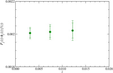
Figure 10: Regular part of axial form factor $P_{f}(z)\phi_{f}(z)f(z)$ as a function of $z$. The two error bars in this figure and Fig. 11 show the statistical and total errors, respectively.

Figure 10 shows the regular part of the axial form factor $P_{f}(z)\phi_{f}(z)f(z)$, which is to be expanded in $z$. We observe rather mild $z$ dependence of all form factors. While there is no clear sign of curvature in our simulation region, we employ a quadratic form $N_{f}\!=\!N_{g}\!=\!N_{{\mathcal{F}}_{1}}\!=\!N_{{\mathcal{F}}_{2}}\!=\!2$ to safely suppress the truncation error. Among twelve coefficients, constants $a_{{{\mathcal{F}}_{1}},0}$ and $a_{{{\mathcal{F}}_{2}},0}$ are fixed to fulfill the kinematical constraints (35) at $w=1$, where $z\!=\!0$ and the linear and quadratic terms in the $z$-parameter expansion (41) vanish, and (36) at ${w_{\rm max}}$, where $z\!\sim\!0.05$ is well below unity, and hence the constant term gives rise to a large contribution to ${{\mathcal{F}}_{2}}$. To be consistent with the unitarity bound (46), we impose the bound $|a_{F,k}|\!\leq\!1$ ($k\!=\!0,1,2$) for all form factors $F\!=\!g,f,{{\mathcal{F}}_{1}}$ and ${{\mathcal{F}}_{2}}$.

Table 7: BGL parametrization (41) of form factors $g$, $f$, ${{\mathcal{F}}_{1}}$ and ${{\mathcal{F}}_{2}}$. The parameters $a_{{{\mathcal{F}}_{1}},0}$ and $a_{{{\mathcal{F}}_{2}},0}$ are fixed from other parameters to satisfy kinematical constraints (35) and (36), respectively.

. $F$ $g$ $f$ ${{\mathcal{F}}_{1}}$ ${{\mathcal{F}}_{2}}$ $a_{F,0}$ 0.0291(18) 0.01198(19) 0.002006(31) 0.0484(16) $a_{F,1}$ $-$0.045(35) 0.018(11) 0.0013(41) $-$0.059(87) $a_{F,2}$ $-$1.0(1.7) $-$0.10(45) $-$0.03(21) $-$0.9(1.1)

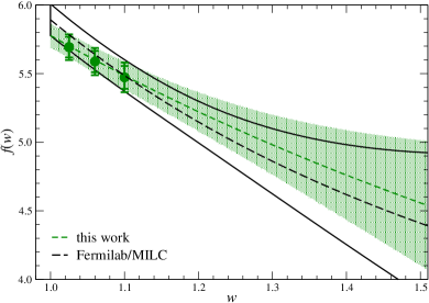
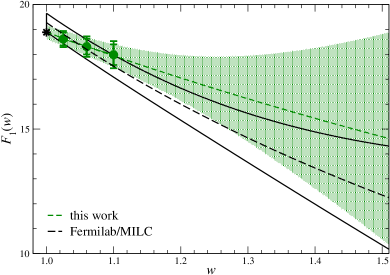
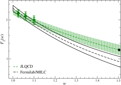
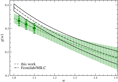
Figure 11: BGL parametrization (green band) of the synthetic data (green circles) in the whole semileptonic region $1\!\leq\!w\!\lesssim\!1.5$. The top-left, top-right, bottom-left and bottom-right panels show $f(w)$, ${{\mathcal{F}}_{1}}(w)$, ${{\mathcal{F}}_{2}}(w)$ and $g(w)$, respectively. We also plot the parametrization by Fermilab/MILC Bazavov et al. (2022) by the open black bands. The stars in the panels for ${{\mathcal{F}}_{1}}$ and ${{\mathcal{F}}_{2}}$ represent the values fixed from the kinematical constraints (35) and (36), respectively.

Table 7 shows fit results, which describe the synthetic data with an acceptable value of $\chi^{2}/{\rm d.o.f.}\!=\!0.51$. We confirm the unitarity bound for the axial vector channel as $\sum_{k=0}^{N_{f}}|a_{f,k}|^{2}+\sum_{k=0}^{N_{{\mathcal{F}}_{1}}}|a_{{{\mathcal{F}}_{1}},k}|^{2}=0.012(96)$, which is poorly saturated by $B\!\to\!D^{*}\ell{\nu_{\ell}}$. The bounds for other channels are satisfied as $\sum_{k=0}^{N_{g}}|a_{g,k}|^{2}=1.0(3.5)$ and $\sum_{k=0}^{N_{{\mathcal{F}}_{2}}}|a_{{{\mathcal{F}}_{2}},k}|^{2}=0.9(2.1)$. The large uncertainty comes from the poorly-determined quadratic coefficients. The sums up to the linear term, $\sum_{k=0}^{1}|a_{g,k}|^{2}=0.0029(31)$ and $\sum_{k=0}^{1}|a_{{{\mathcal{F}}_{2}},k}|^{2}=0.006(10)$, suggest that the unitarity bound is rather weak as mentioned above.

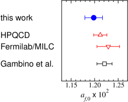
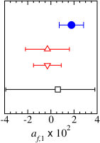
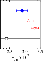
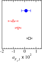
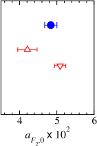
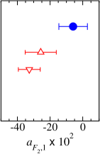
Figure 12: Comparison of expansion coefficients for BGL parametrization (41). Our results are plotted as filled blue circles. Open red triangles are obtained by HPQCD (triangles up) Harrison and Davies (2023) and Fermilab/MILC (triangles down) Bazavov et al. (2022). We also plot results from a recent phenomenological analysis of the Belle data Waheed et al. (2019) as open black squares Gambino et al. (2019). Since all these studies impose the kinematical constraint (35) leading to $a_{{{\mathcal{F}}_{1}},0}\!\propto\!a_{f,0}$, we omit a panel for $a_{{{\mathcal{F}}_{1}},0}$.

The BGL parametrization and synthetic data of the form factors are plotted in Fig. 11. We observe reasonable consistency with the Fermilab/MILC results Bazavov et al. (2022) except the vector form factor $g(w)$ near zero-recoil and the axial form factor ${{\mathcal{F}}_{2}}$ extrapolated to large recoils. This can be seen in a more detailed comparison of the expansion coefficients in Fig. 12, where there is slight tension in $a_{g,0}$, $a_{g,1}$ and $a_{{{\mathcal{F}}_{1}},1}$. Recent HPQCD results show better consistency with ours, except for $a_{{{\mathcal{F}}_{1}},1}$ and $a_{{{\mathcal{F}}_{2}},0}$.

In the same figure, we also plot a phenomenological estimate Gambino et al. (2019) from the BGL parametrization to the same order ($N_{f}\!=\!N_{g}\!=\!N_{{\mathcal{F}}_{1}}\!=\!2$) of the Belle data Waheed et al. (2019) combined with a lattice input of the FLAG average of $h_{A_{1}}(1)\!\propto\!f(1)$ Aoki et al. (2020). The phenomenological result of $a_{f,0}$ is well determined and shows good consistency with lattice results, simply because it is mainly fixed from the lattice input. Other poorly determined coefficients suggest the importance of lattice calculations to obtain controlled BGL parametrization.

On the other hand, the slope $a_{F_{1},1}$ is well determined from the phenomenological analysis of the experimental data, which are precise at large recoils. This study observes a reasonable agreement in $a_{F_{1},1}$ and, hence, in the differential decay rate as discussed in the next subsection (see Fig. 13). We note, however, that the Fermilab/MILC and HPQCD studies reported tension in the $w$ dependence of the differential decay rate with experiment.

Since ${{\mathcal{F}}_{2}}$ describes the contribution suppressed by $m_{\ell}^{2}$ to the decay rate (40), its expansion coefficients are poorly constrained by the experimental data for the light lepton channels $B\!\to\!D^{*}\ell{\nu_{\ell}}$ ($\ell\!=\!e,\mu$). The lattice determination of ${{\mathcal{F}}_{2}}$ is, therefore, helpful towards a precision new physics search using the $\tau$ channel. Through numerical integration of Eq. (40) for $\ell\!=\!e,\mu$ and $\tau$ with fit results in Table 7, we obtain a pure SM value

$$R(D^{*}) = 0.252(22),$$ (51)

which does not resort to phenomenological models nor experimental data. This can be improved as $R(D^{*})\!=\!0.252(+0.009/\!\!-\!\!0.016)$ by imposing the unitarity bound (46) on the expansion coefficients. These are consistent with Fermilab/MILC and HPQCD estimates, 0.265(13) and 0.279(13), respectively, and to be compared with the experimental average 0.295(14) Amhis et al. (2023). For a more precise and reliable estimate of $R(D^{*})$, it is helpful to simulate larger recoils as well as resolving the tensions in $a_{{{\mathcal{F}}_{2}},\{0,1\}}$ shown in Fig. 12.

IV.2 Fit including Belle data

In this subsection, we carry out a simultaneous fit to our lattice and Belle data to estimate ${|V_{cb}|}$. The differential decay rate with respect to $w$ and three decay angles $\theta_{l}$, $\theta_{v}$ and $\chi$ is given as

$$\frac{d\Gamma}{dwd{\cos[\theta_{\ell}]}d{\cos[\theta_{v}]}d\chi} = \frac{3G_{F}^{2}}{1024\pi^{4}}|V_{cb}|^{2}\eta_{\rm EW}^{2}M_{B}r^{2}\sqrt{w^{2}-1}\,q^{2}$$ (52)

$$\hskip 11.38109pt\times\left\{(1-{\cos[\theta_{\ell}]})^{2}{\sin^{2}[\theta_{v}]}H_{+}^{2}(w)+(1+{\cos[\theta_{\ell}]})^{2}{\sin^{2}[\theta_{v}]}H_{-}^{2}(w)\right.$$

$$\hskip 28.45274pt\left.+4{\sin^{2}[\theta_{\ell}]}{\cos^{2}[\theta_{v}]}H_{0}^{2}(w)-2{\sin^{2}[\theta_{\ell}]}{\sin^{2}[\theta_{v}]}\cos[2\chi]H_{+}(w)H_{-}(w)\right.$$

$$\hskip 28.45274pt\left.-4{\sin[\theta_{\ell}]}(1-{\cos[\theta_{\ell}]}){\sin[\theta_{v}]}{\cos[\theta_{v}]}\cos[\chi]H_{+}(w)H_{0}(w)\right.$$

$$\hskip 28.45274pt\left.+4{\sin[\theta_{\ell}]}(1+{\cos[\theta_{\ell}]}){\sin[\theta_{v}]}{\cos[\theta_{v}]}\cos[\chi]H_{-}(w)H_{0}(w)\right\}$$

with the helicity amplitudes given in (37) and (38). For a simultaneous fit with the Belle data for $B^{0}\!\to\!D^{*-}\ell^{+}{\nu_{\ell}}$ $(\ell\!=\!e,\mu)$ in Ref. Waheed et al. (2019), we set $m_{\ell}\!=\!0$, and include the Coulomb factor $(1+\alpha\pi)$ in the right-hand side. The decay angles are chosen the same as for the Belle paper, where the full kinematical distribution is described by four differential decay rates $d\Gamma/dw$, $d\Gamma/d{\cos[\theta_{\ell}]}$, $d\Gamma/d{\cos[\theta_{v}]}$ and $d\Gamma/d\chi$, which are integrated over the other three variables. The differential decay rates are provided at ten equal-size bins in the range of each variable, $w\!\in\![1.0,1.5]$, $\cos[\theta_{\{\ell,v\}}]\!\in\![-1,1]$ and $\chi\!\in\![-\pi,\pi]$.

To estimate ${|V_{cb}|}$, we fit our synthetic data of the form factors to the BGL parametrization (41) alongside the Belle data of the calculated differential decay rates where the expansion coefficients $a_{\{g,f,{{\mathcal{F}}_{1}},{{\mathcal{F}}_{2}}\},\{0,1,2\}}$ are shared parameters and ${|V_{cb}|}$ is an additional parameter determined from the fit. The expression (40) is used for $d\Gamma/dw$. We calculate $d\Gamma/d\cos[\theta_{\{l,v\}}]$ and $d\Gamma/d\chi$ by analytically integrating over two other decay angles and by numerically integrating over $w$ via Simpson’s rule with 800 steps within each bin as in the Belle paper Waheed et al. (2019).

Table 8: Fit results of simultaneous fit to our lattice and Belle data.

. $F$ $g$ $f$ ${{\mathcal{F}}_{1}}$ ${{\mathcal{F}}_{2}}$ $a_{F,0}$ 0.02896(84) 0.01196(18) 0.002003(30) 0.0489(14) $a_{F,1}$ $-$0.050(23) 0.0227(92) 0.0040(14) $-$0.018(24) $a_{F,2}$ $-$1.0(1.9) $-$0.46(24) $-$0.040(27) $-$1.0(2.0)

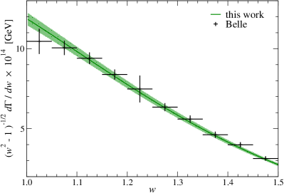
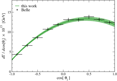
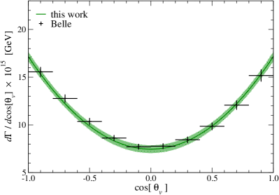
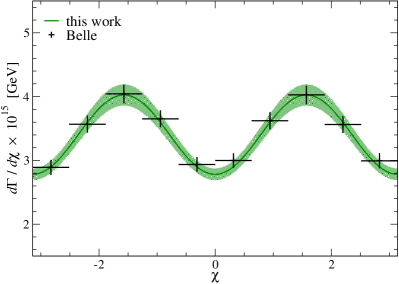
Figure 13: Differential decay rate with respect to recoil parameter, $d\Gamma/dw$ (top-left panel), and three decay angles, $d\Gamma/d\cos[\theta_{\ell}]$ (top-right panel), $d\Gamma/d\cos[\theta_{v}]$ (bottom-left panel) and $d\Gamma/d\chi$ (bottom-right panel). We divide $d\Gamma/dw$ by a phase space factor $\sqrt{w^{2}-1}$ to make its $w$-dependence milder and monotonous. The symbols show Belle results, whereas the green band is reproduced from our simultaneous fit to our lattice and Belle data.

Our results for the expansion coefficients are summarized in Table 8. These are consistent with those in Table 7, which are obtained without the experimental data, with slightly smaller uncertainty. We obtain

$${|V_{cb}|}=39.19(90)\times 10^{-3},$$ (53)

which is in good agreement with the previous determination from the exclusive decay (5). In contrast to previous lattice studies, as shown in Fig. 13, we observe consistency between our lattice and Belle data leading to an acceptable value of $\chi^{2}/{\rm d.o.f.}\!\sim\!0.90$. Towards the resolution of the ${|V_{cb}|}$ tension, we need a more detailed analysis taking care of, for instance, bias in ${|V_{cb}|}$ discussed in Refs. Gambino et al. (2019); Ferlewicz et al. (2021) due to D’Agostini effects D’Agostini (1994) and the strong systematic correlation of experimental data. That analysis is left for future work.

V Conclusion

In this article, we present our calculation of the $B\!\to\!D^{*}\ell{\nu_{\ell}}$ semileptonic form factors in 2+1-flavor lattice QCD. The Möbius domain-wall action is employed for all relevant quark flavors to simulate lattices of cutoffs up to 4.5 GeV with chiral symmetry preserved to good accuracy. This removes the leading $O(a)$ discretization errors and explicit renormalization is not necessary to calculate the SM form factors through the correlator ratios. The ground state saturation of the correlator ratios is carefully studied by simulating four source-sink separations. The bottom quark mass is limited to $m_{b}\!\leq\!0.7a^{-1}$ to suppress $O(a^{2})$ and higher discretization error. Note also that the chiral logarithm is suppressed by the small $D^{*}$ – $D$ mass splitting squared. As a result, the lattice spacing and quark mass dependence turns out to be mild in our simulation region leading to good control of the continuum and chiral extrapolation. We find finite size effects to be small by direct simulations of two volumes at our smallest pion mass.

One of the main results is the synthetic data of the form factors $g$, $f$, ${{\mathcal{F}}_{1}}$ and ${{\mathcal{F}}_{2}}$ in the relativistic convention at three reference values of the recoil parameter $w\!=\!1.025$, 1.060 and 1.100, which can be used in future analyses to determine ${|V_{cb}|}$ and to search for new physics. Through the BGL parametrization, we obtain $R(D^{*})\!=\!0.252(22)$ in the SM. A combined analysis with the Belle data yields ${|V_{cb}|}\!=\!39.19(90)\times 10^{-3}$. These are consistent with previous lattice studies. However, the expansion coefficients for $g$, ${{\mathcal{F}}_{1}}$ and ${{\mathcal{F}}_{2}}$ show significant tension among lattice studies. In particular, our slope for ${{\mathcal{F}}_{1}}$ is slightly larger and consistent with a phenomenological analysis of the Belle data. As a result, our data show better consistency with the Belle data in the differential decay rates.

High statistics simulations on finer lattices would be helpful in resolving this tension. Simulating larger recoils can lead to a better estimate of $R(D^{*})$ as well as more detailed comparison with experiment in a wide range of the recoil parameter to search for new physics. In order to resolve the ${|V_{cb}|}$ tension, it would also be very helpful to study the inclusive decay on the lattice for more direct comparison of the exclusive and inclusive analyses in the same simulations Hashimoto (2017). While it is an ill-posed problem to calculate the relevant hadronic tensor from discrete lattice data on a finite volume, a joint project of the JLQCD and RBC/UKQCD Collaborations along a strategy proposed in Ref. Hansen et al. (2017); Gambino and Hashimoto (2020) is in progress Barone et al. (2023a); Kellermann et al. (2023); Barone et al. (2023b) towards a realistic study of $B\!\to\!X_{c}\ell{\nu_{\ell}}$.