Specifying and Solving Robust Empirical Risk Minimization Problems Using CVXPY

Abstract

We consider robust empirical risk minimization (ERM), where model parameters are chosen to minimize the worst-case empirical loss when each data point varies over a given convex uncertainty set. In some simple cases, such problems can be expressed in an analytical form. In general the problem can be made tractable via dualization, which turns a min-max problem into a min-min problem. Dualization requires expertise and is tedious and error-prone. We demonstrate how CVXPY can be used to automate this dualization procedure in a user-friendly manner. Our framework allows practitioners to specify and solve robust ERM problems with a general class of convex losses, capturing many standard regression and classification problems. Users can easily specify any complex uncertainty set that is representable via disciplined convex programming (DCP) constraints.

1 Robust empirical risk minimization

Robust optimization is used in mathematical optimization, statistics, and machine learning, to handle problems where the data is uncertain. In this note we consider the robust empirical risk minimization (RERM) problem

$$\begin{array}[]{ll}\mbox{minimize}&\sum_{i=1}^{n}\sup_{x_{i}\in\mathcal{X}_{i}}f(x_{i}^{T}\theta-y_{i})\\ \mbox{subject to}&\theta\in\Theta,\end{array}$$ (1)

with variable $\theta\in{\mbox{\bf R}}^{d}$. Here, $\Theta\subseteq{\mbox{\bf R}}^{d}$ is closed and convex, $\mathcal{X}_{i}\subset{\mbox{\bf R}}^{d}$ is compact and convex for each $i=1,\ldots,n$, $f:{\mbox{\bf R}}\to{\mbox{\bf R}}$ is convex and $\{x_{i},y_{i}\}_{i=1}^{n}$ is a dataset. The objective is to find $\theta\in\Theta$ that minimizes the worst-case value of $\sum_{i=1}^{n}f(x_{i}^{T}\theta-y_{i})$ over all possible $x_{i}$ in the given uncertainty sets $\mathcal{X}_{i}$. Beyond convexity, we will assume that $f$ is either non-increasing, or $f$ is non-decreasing on ${\mbox{\bf R}}_{+}$ and a function of the absolute value of its argument, i.e., $f(z)=f(|z|)$.

Examples.

Our assumptions capture a wide range of loss functions in both regression and classification, including the following.

• Finite $p$-norm loss. $f(z)=|z|^{p}$ for $1\leq p<\infty$.

• Huber loss. $f(z)=\frac{1}{2}z^{2}$ for $|z|\leq\delta$, and $f(z)=\delta|z|-\frac{\delta^{2}}{2}$ for $|z|>\delta$, where $\delta>0$ is a parameter.

• Hinge loss. $f(z)=\max(0,1-z)$.

• Logistic loss. $f(z)=\log(1+\exp(-z))$.

• Exponential loss. $f(z)=\exp(-z)$.

Our formulation includes the case of using hinge, logistic, or exponential loss for binary classification, by solving (1) with the transformed dataset $\{y_{i}x_{i},0\}$.

1.1 Solving RERM problems

The problem (1) is convex, but not immediately tractable because of the suprema appearing in the worst-case loss terms. It can often be transformed to an explicit tractable form that does not include suprema.

Analytical cases.

In some simple cases we can directly work out a tractable expression for the worst-case loss. As a simple example, consider $\mathcal{X}_{i}=\{x_{i}\mid\|x_{i}-\tilde{x}_{i}\|_{2}\leq\rho\}$, where $\rho>0$. When $f$ is non-increasing, the worst-case loss term is

$$\sup_{x_{i}\in\mathcal{X}_{i}}f(x_{i}^{T}\theta-y_{i})=f(\tilde{x}_{i}^{T}\theta-y_{i}-\rho\|\theta\|_{2}).$$

When $f$ is non-decreasing on ${\mbox{\bf R}}_{+}$ with $f(z)=f(|z|)$, the worst-case loss term is

$$\sup_{x_{i}\in\mathcal{X}_{i}}f(x_{i}^{T}\theta-y_{i})=f(|\tilde{x}_{i}^{T}\theta-y_{i}|+\rho\|\theta\|_{2}).$$

Both righthand sides are explicit convex expressions that comply with the disciplined convex programming (DCP) rules. This means they can be directly typed into domain specific languages (DSLs) for convex optimization such as CVXPY [DB16].

Dualization.

For more complex uncertainty sets the problem (1) can still be transformed to a tractable form, using dualization of the suprema apprearing in the worst-case loss terms. This dualization process converts the suprema in (1) to infima, so that the problem can be solved by standard methods as a single minimization problem. Unfortunately, this dualization procedure is cumbersome and error-prone. Many practitioners are not well versed in this procedure, limiting its use to experts. Moreover, a key step in this procedure involves writing down a conic representation of $\mathcal{X}_{i}$. Such a calculation is antithetical to the spirit of DSLs such as CVXPY, which were introduced precisely to alleviate users of this burden.

Automatic dualization via CVXPY.

In this note we show how CVXPY can be used to conveniently solve (1) with just a few lines of code, even when the uncertainty sets $\mathcal{X}_{i}$ are complicated. We also demonstrate how DSP, a recent DSL for disciplined saddle programming [SLB23] that is based on CVXPY, can solve the RERM problem (1) with the same ease and convenience. In both approaches no explicit dualization is needed, and the code is short and naturally follows the math. We demonstrate our approach with a synthetic regression example that, however, uses real data, where the uncertainty sets are intervals intersected with a Euclidean ball.

1.2 Previous and related work

Robust optimization and saddle problems.

Robust optimization is an approach that takes into account uncertainty, variability or missing-ness of problem parameters [BTEGN09]. Saddle problems are robust optimization problems that include the partial supremum or infimum of convex-concave saddle functions. While (1) is not a priori a saddle problem, we can solve it via DSP [SLB23], a recently introduced DSL for saddle programming.

RERM.

In machine learning and statistics, it is common to learn a robust predictor or classifier by solving (1) with appropriate choices of $f,\mathcal{X}_{i}$ [EGL97, XCM08, XCM09, BBC11]. When each $\mathcal{X}_{i}$ has benign structure, then (1) admits convenient reformulation for many choices of $f$ [BV04]. As an example, such reformulations have been applied to learn linear regression functions when the feature matrix has missing data, and the features are known to lie with high probability in an ellipsoid, so that (1) is easily written as an SOCP [SBS06, AFG22]. However, when $\mathcal{X}_{i}$ is not a simple set such as an ellipsoid or box, then prior techniques reformulate (1) by writing $\mathcal{X}_{i}$ in conic form and then dualizing [BTEGN09].

2 Reformulating the RERM problem

Throughout, our only requirement on the uncertainty sets $\mathcal{X}_{i}$ is that each is a compact, convex set that can be expressed via DCP constraints. This includes canonical scenarios, such as when $\mathcal{X}_{i}$ is a polytope, or is a norm ball centered at a nominal value. But it also includes many complex uncertainty sets, such as the intersection of a norm ball and a polytope. We now reformulate (1) in a manner that permits easy specification and solution via CVXPY, under various monotonicity assumptions on $f$. Recall that the support function of a non-empty closed convex set $C$ is given by $\mathcal{S}_{C}(\theta)=\sup\{x^{T}\theta:x\in C\}$, which is a fundamental object in convex analysis [BV04].

Introducing the epigraph variables $c\in{\mbox{\bf R}}^{n}$, the problem (1) is straightforwardly equivalent to

$$\begin{array}[]{ll}\mbox{minimize}&\sum_{i=1}^{n}c_{i}\\ \mbox{subject to}&\theta\in\Theta,\\ &\sup_{x_{i}\in\mathcal{X}_{i}}f(x_{i}^{T}\theta-y_{i})\leq c_{i},\quad i=1,\ldots,n.\end{array}$$ (2)

with variables $c\in{\mbox{\bf R}}^{n},\theta\in{\mbox{\bf R}}^{d}$. We now use the assumptions on $f$ to rewrite the constraints $\sup_{x_{i}\in\mathcal{X}_{i}}f(x_{i}^{T}\theta-y_{i})\leq c_{i}$ in a tractable form.

Loss $f$ is non-increasing.

If $f$ is non-increasing, then introducing an auxiliary variable $z_{i}$ shows that

$$\sup_{x_{i}\in\mathcal{X}_{i}}f(x_{i}^{T}\theta-y_{i})\leq c_{i} \iff f\left(\inf_{x_{i}\in\mathcal{X}_{i}}x_{i}^{T}\theta-y_{i}\right)\leq c_{i}$$

$$\iff \inf_{x_{i}\in\mathcal{X}_{i}}x_{i}^{T}\theta-y_{i}\geq z_{i},\quad f(z_{i})\leq c_{i}$$

$$\iff \sup_{x_{i}\in\mathcal{X}_{i}}-x_{i}^{T}\theta+y_{i}\leq-z_{i},\quad f(z_{i})\leq c_{i}.$$

So, after eliminating the epigraph variable $c$ from (2), we have shown (1) is equivalent to

$$\begin{array}[]{llll}\mbox{minimize}&\sum_{i=1}^{n}f(z_{i})\\ \mbox{subject to}&\theta\in\Theta,\\ &\mathcal{S}_{\mathcal{X}_{i}}(-\theta)+y_{i}\leq-z_{i},\quad i=1,\ldots,n,\end{array}$$ (3)

with variables $z\in{\mbox{\bf R}}^{n},\theta\in{\mbox{\bf R}}^{d}$. Typical classification losses, such as the hinge, logistic and exponential losses, are non-increasing.

Loss $f$ is non-decreasing on ${\mbox{\bf R}}_{+}$ and $f(a)=f(|a|)$.

If $f$ is monotone on nonnegative arguments, and depends only on its argument through the absolute value, then introducing the auxiliary variable $z_{i}$ shows that

$$\sup_{x_{i}\in\mathcal{X}_{i}}f(x_{i}^{T}\theta-y_{i})\leq c_{i} \iff f\left(\sup_{x_{i}\in\mathcal{X}_{i}}|x_{i}^{T}\theta-y_{i}|\right)\leq c_{i}$$

$$\iff \sup_{x_{i}\in\mathcal{X}_{i}}|x_{i}^{T}\theta-y_{i}|\leq z_{i},\quad f(z_{i})\leq c_{i}$$

$$\iff \sup_{x_{i}\in\mathcal{X}_{i}}x_{i}^{T}\theta-y_{i}\leq z_{i},\quad\sup_{x_{i}\in\mathcal{X}_{i}}-x_{i}^{T}\theta+y_{i}\leq z_{i},\quad f(z_{i})\leq c_{i}.$$

So, after eliminating the epigraph variable $c$ from (2), we have shown (1) is equivalent to

$$\begin{array}[]{llll}\mbox{minimize}&\sum_{i=1}^{n}f(z_{i})\\ \mbox{subject to}&\theta\in\Theta,\\ &\mathcal{S}_{\mathcal{X}_{i}}(\theta)-y_{i}\leq z_{i},\quad i=1,\ldots,n,\\ &\mathcal{S}_{\mathcal{X}_{i}}(-\theta)+y_{i}\leq z_{i},\quad i=1,\ldots,n,\end{array}$$ (4)

with variables $z\in{\mbox{\bf R}}^{n},\theta\in{\mbox{\bf R}}^{d}$. Typical regression losses, such as $p$-norm and Huber losses, satisfy this requirement on $f$.

CVXPY code.

The robust constraints in (3) and (4) include suprema over $\mathcal{X}_{i}$ of bilinear forms involving $x_{i},\theta$. While this ostensibly requires dualization to handle, the CVXPY transform SuppFunc allows one to easily specify the support function $\mathcal{S}_{C}(\theta)$ of a set $C$ created via DCP constraints. Since this function is already implemented in CVXPY, we can directly specify the robust constraints in (3) and (4) without additional reformulation or dualization. As an example, we depict below the CVXPY code that specifies and solves (4) with $f=|\cdot|^{2}$ and $\Theta={\mbox{\bf R}}^{d}$, which is a robust least squares problem. For convenience, we assume $y$ has already been specified as y.

⬇

1import cvxpy as cp

2from cvxpy.transforms.suppfunc import SuppFunc

3

4theta, z = cp.Variable(d), cp.Variable(n)

5constraints = []

6

7for i in range(n):

8 # Create variables for uncertainty set

9 x1, x2 = cp.Variable(d), cp.Variable(d)

10

11 # Constructs uncertainty set containing x (filled in by user)

12 local_constraints1 = []

13 local_constraints2 = []

14

15 # Implement the support function of the uncertainty set

16 G1 = SuppFunc(x1, local_constraints1)(theta)

17 G2 = SuppFunc(x2, local_constraints2)(-theta)

18

19 # Store robust constraints

20 constraints.append(G1 - y[i] <= z[i])

21 constraints.append(G2 + y[i] <= z[i])

22

23obj = cp.Minimize(cp.sum_squares(z))

24prob = cp.Problem(obj, constraints)

25prob.solve()

To fully specify the problem, the user only needs to describe the uncertainty set $\mathcal{X}_{i}$ for each $i=1,\ldots,n$ in Lines 12-13, in terms of the x1 and x2 instantiated in Line 9. This is done exactly as one would typically do for any Variable in CVXPY. If, for example, $\mathcal{X}_{i}$ was the intersection of the Euclidean unit ball, the non-negative orthant, and the set of vectors whose first coordinate is 0.25, then replacing Lines 12-13 with the code block below is sufficient.

⬇

12local_constraints1 = [x1 >= 0, cp.sum_squares(x1) <= 1, x1[0] == 0.25]

13local_constraints2 = [x2 >= 0, cp.sum_squares(x2) <= 1, x2[0] == 0.25]

This manner of expressing $\mathcal{X}_{i}$ is thus natural, user-friendly and directly follows the math.

Alternatively, one may recognize that the constraints in (3) and (4) include the partial suprema of a convex-concave saddle function. Since DSP was designed to solve saddle problems, and a bilinear function is an atom in DSP, we can use DSP to solve (3) and (4) with the same convenience and ease. All that is required is importing DSP via from dsp import *, and replacing lines 8-17 above with the code block below.

⬇

1# Creating local variables for uncertainty set

2x1, x2 = LocalVariable(d), LocalVariable(d)

3

4# Create bilinear form of theta and x

5g1, g2 = saddle_inner(theta, x1), saddle_inner(-theta, x2)

6

7# Constructs uncertainty set containing x (filled in by user)

8local_constraints1 = []

9local_constraints2 = []

10

11# Take suprema over x

12G1 = saddle_max(g1, local_constraints1)

13G2 = saddle_max(g2, local_constraints2)

3 Example

We consider the problem of predicting nightly Airbnb rental prices in London, from different features such as coordinates, distance from city center, and neighborhood restaurant quality index. We will consider a simulated hypothetical case where we do not have full acess to the rentals’ location. We will use robust regression to handle the uncertain location features. We can then use uncertainty sets for the unknown locations, allowing us to illustrate the ease of specifying RERM problems with our framework. This example is artificial, but does use real original data. We do not advocate using robust regression in particular for this problem; replacing each unknown location with a center of the uncertainty set performs nearly as well as the best robust regression method, and is much simpler.

Data.

We begin with a curated dataset from London [GN21], and remove rentals with prices exceeding 1000 Euros and those located more than 7 km from the city center, resulting in a dataset of 3400 rows and 20 columns. We then remove categorical features and randomly sub-sample to obtain a training set with 1000 data points and test data set with 500 data points. The training feature matrix is $X\in{\mbox{\bf R}}^{1000\times 9}$, with rows $x_{i}^{T}$. The first two columns of $X$ correspond to the longitude and latitude respectively. Our baseline predictor of rental price is a simple linear ordinary least squares (OLS) regression based on all 9 features. Its test RMS error is 138 euros.

Hidden location features.

To illustrate our method, we imagine a case where rental owners have elected to not release the exact longitude and latitude of their properties. (While not identical to this example, Airbnb does in fact mask rental locations.) We grid London into 1 km by 1 km squares, and for each rental only give the square $S_{i}$ it is located in. This generates an uncertainty set for data point $i$ given by

$$\mathcal{X}_{i}^{S}=\{x\in{\mbox{\bf R}}^{9}\mid x_{1:2}\in S_{i},~{}x_{3:9}=X^{i}_{3:9}\}.$$

We also know the distance of each rental from the city center $c\in{\mbox{\bf R}}^{2}$, denoted by $d_{i}$. Using this, we can consider a more refined uncertainty set

$$\mathcal{X}_{i}^{S\cap D}=\mathcal{X}_{i}^{S}\cap D_{i},$$

where $D_{i}=\{x\in{\mbox{\bf R}}^{9}\mid\|x_{1:2}-c\|_{2}\leq d_{i}\}$. See figure 1 for a visualization of these uncertainty sets.

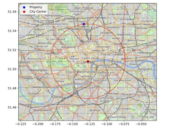
Figure 1: A visualization of $D_{i}$ and $S_{i}$ for a particular rental $i$. The large disk around the red dot corresponds to $D_{i}$. The square containing the blue dot corresponds to $S_{i}$. The overlap of the square and the disk corresponds to $D_{i}\cap S_{i}$.

We solve (4) with squared loss $f=|\cdot|^{2}$ and the two choices of the uncertainty sets described above. These choices correspond to using square or disk-intersected-with-square uncertainty sets for the missing coordinates. Note that the square uncertainty set combined with the quadratic loss is a special case where we can derive an analytical form for the worst-case loss. However, the analytical form is lost once we intersect the square with the disk.

Comparing the methods.

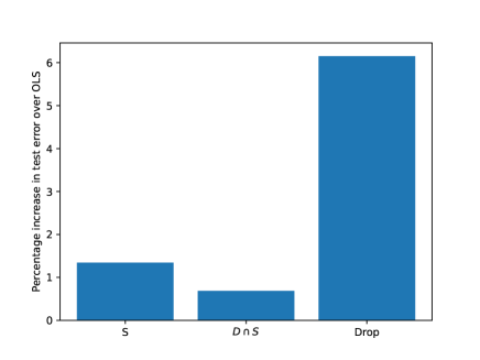
Figure 2: Excess test error in the Airbnb price prediction experiment.

We depict the performance of the two RERM predictors, as well as a predictor that completely ignores coordinate information, in figure 2. Our performance metric is the mean squared error on the test set, in excess of the baseline OLS predictor trained on $X$ without any missing entries.

We observe that the dropping scheme, denoted as Drop in figure 2, performs the worst. The robust predictors that use square uncertainty sets (denoted as $S$) and the intersected uncertainty sets (denoted as $S\cap D$) outperform the others. The robust predictor that uses uncertainty sets $S\cap D$ outperforms the robust predictor that uses only $S$. Indeed, its performance is nearly as good as the OLS predictor baseline that has access to all the columns of $X$. These intersected uncertainty sets are complex and do not admit the sort of convenient reformulation afforded by using square or disk uncertainty sets. Yet, our framework allows us to handle these uncertainty sets conveniently, and hence obtain less conservative predictors.

References

- [EGL97] Laurent El Ghaoui and Hervé Lebret “Robust solutions to least-squares problems with uncertain data” In SIAM Journal on matrix analysis and applications 18.4 SIAM, 1997, pp. 1035–1064
- [BV04] S. Boyd and L. Vandenberghe “Convex Optimization” Cambridge University Press, 2004
- [SBS06] Pannagadatta K. Shivaswamy, Chiranjib Bhattacharyya and Alexander J. Smola “Second Order Cone Programming Approaches for Handling Missing and Uncertain Data” In Journal of Machine Learning Research 7.47, 2006, pp. 1283–1314
- [XCM08] Huan Xu, Constantine Caramanis and Shie Mannor “Robust Regression and Lasso” In Advances in Neural Information Processing Systems 21 Curran Associates, Inc., 2008
- [BTEGN09] Aharon Ben-Tal, Laurent El Ghaoui and Arkadi Nemirovski “Robust optimization” Princeton university press, 2009
- [XCM09] Huan Xu, Constantine Caramanis and Shie Mannor “Robustness and Regularization of Support Vector Machines” In Journal of Machine Learning Research 10.51, 2009, pp. 1485–1510
- [BBC11] Dimitris Bertsimas, David Brown and Constantine Caramanis “Theory and applications of robust optimization” In SIAM review 53.3 SIAM, 2011, pp. 464–501
- [DB16] Steven Diamond and Stephen Boyd “CVXPY: A Python-embedded modeling language for convex optimization” In Journal of Machine Learning Research 17.83, 2016, pp. 1–5
- [GN21] Kristóf Gyódi and Łukasz Nawaro “Determinants of Airbnb prices in European cities: A spatial econometrics approach” In Tourism Management 86, 2021, pp. 104319
- [AFG22] Alireza Aghasi, MohammadJavad Feizollahi and Saeed Ghadimi “RIGID: Robust Linear Regression with Missing Data” In arXiv preprint arXiv:2205.13635, 2022
- [SLB23] Philipp Schiele, Eric Luxenberg and Stephen Boyd “Disciplined Saddle Programming” In arXiv preprint arXiv:2301.13427, 2023