Dependence of galactic bars on the tidal density field in the SDSS

Abstract

As a key driver of the secular evolution of disc galaxies, bar formation is potentially linked to the surrounding tidal field. We systematically investigate the dependence of bars on both the small (${<}2\,\mathrm{Mpc}/h$) and large (${>}5\,\mathrm{Mpc}/h$) scale tidal fields using galaxies observed between $0.01{<}z{<}0.11$ by the Sloan Digital Sky Survey (SDSS). We characterise bar strength using the ellipticity of the isophote that corresponds to each bar, $e_{\mathrm{bar}}$, derived from its galaxy image after subtracting the 2D disc component. We demonstrate the efficacy of our bar detection method by performing an extensive comparison with the visual identifications from SDSS and the DESI Legacy Surveys. Using the Yang et al. SDSS group catalogue, we confirm the results from a recent study that the average $e_{\mathrm{bar}}$ of galaxies within interacting clusters is higher than that within isolated ones at $0.01{<}z{<}0.06$, but this small-scale tidal enhancement of bars disappears after we increase the cluster sample by a factor of five to $z{=}0.11$. On large scales, we explore the dependence of $e_{\mathrm{bar}}$ on $\alpha_{5}$, the tidal anisotropy of the density field defined over $5\,\mathrm{Mpc}/h$. We do not detect any such dependence for $98\%$ of the galaxies with $\alpha_{5}{<}10$. Intriguingly, among the $2\%$ with $\alpha_{5}{\geq}10$, we detect some hint of a boost in bar strength in the underdense regions and a suppression in the overdense regions. Combining our results on both scales, we conclude that there is little evidence for the tidal dependence of bar formation in the local Universe, except for the extremely anisotropic environments.

1 Introduction

As the most common non-axisymmetric structure in spiral galaxies, bars serve as a potent agent for redistributing angular momentum in the disc-halo systems, thereby driving the secular evolution of disc galaxies (Kormendy & Kennicutt, 2004; Sellwood, 2014). N-body simulations have shown that the formation of bars is almost an inevitable consequence of the strong $m{=}2$ instability in disc galaxies, and once formed, bars are believed to be long-lived (but see Bournaud & Combes, 2002). Yet, one third of the discs in the local Universe remain barless (de Vaucouleurs, 1963; Barazza et al., 2008; Aguerri et al., 2009; Nair & Abraham, 2010; Masters et al., 2011). One possibility is that the promotion and/or inhibition of bar-formation instability may depend sensitively on the tidal density environment, which is intimately linked to the halo angular momentum in the $\Lambda$-dominated cold dark matter ($\Lambda$CDM) Universe. In this paper, we develop an automated bar detection method to measure the bar strength for galaxies observed by the Sloan Digital Sky Survey (SDSS; York et al., 2000). By examining the tidal field on both small (${<}2\,h^{-1}\mathrm{Mpc}$) and large (${>}5\,h^{-1}\mathrm{Mpc}$) scales, we aim to systematically search for the tidal dependence of bars in the local Universe.

Despite the lack of a complete theory of bar formation  (see Sellwood, 2014, for a recent review), the basic mechanism is reasonably well understood (Binney & Tremaine, 2008). In the linear regime, self-gravitating cold discs are globally unstable against non-axisymmetric modes (Kalnajs, 1972), resulting in the formation of weak spiral disturbances. In a differentially rotating disc, these initial disturbances grow by successive swing amplifications at the co-rotation radius and reflections off the galactic centre (Toomre, 1981). After a nascent bar emerges out of this feedback loop, it could trap the eccentric stellar orbits and force them to precess coherently, thereby reinforcing the stellar bar (Lynden-Bell, 1979; Earn & Lynden-Bell, 1996). The bar-formation instability generally sets off spontaneously (Hohl, 1971; Ostriker & Peebles, 1973; Lynden-Bell, 1979; Sellwood, 1981; Efstathiou et al., 1982), but can be triggered by an external perturber in mergers or flybys as well (Byrd et al., 1986; Noguchi, 1987, 1988; Gerin et al., 1990; Miwa & Noguchi, 1998; Berentzen et al., 2004; Martinez-Valpuesta et al., 2017; Peschken & Łokas, 2019; Cavanagh et al., 2022). Numerical studies suggested that the presence of a hot “spheroidal” (a massive central bulge or dark matter halo) component may stabilize the disc against bar instability (Ostriker & Peebles, 1973; Efstathiou et al., 1982; Kataria & Das, 2018; Kataria et al., 2020; Jang & Kim, 2023). However, a strong bar can still form in the disc embedded in a massive “live” halo that responds to the stellar components (Hernquist & Weinberg, 1992; Debattista & Sellwood, 2000; Athanassoula, 2002, 2003).

Beyond halo mass, the spin of the dark matter haloes may also affect the formation and growth of bars. By modelling the dynamical friction of a rotating rigid bar inside an isothermal halo, Weinberg (1985) discovered that the halo spin can promote bar growth as the excess torque of the prograde orbits helps increase the rate at which the bar loses its angular momentum. More recently, Saha & Naab (2013) carried out a suite of N-body simulations of barred galaxies living in halos with different amount of spin. Confirming the semi-analytic arguments from Weinberg (1985), they found that the bars form more rapidly and grow stronger in co-rotating haloes with larger spin. During the subsequent secular evolution, bar growth may instead be suppressed in fast-spinning haloes that are capable of replenishing angular momentum to the bar (Long et al., 2014; Collier et al., 2018). Some cosmological hydrodynamic simulations also predict a relatively lower frequency of barred galaxies in fast-spinning haloes (Rosas-Guevara et al., 2022; Izquierdo-Villalba et al., 2022), despite their difficulty in resolving the short bars (Zhao et al., 2020). Yet a high spin of the inner halo could trigger an earlier buckling, producing a more pronounced boxy/peanut shape of the final bar (Kataria & Shen, 2022). Therefore, despite the lack of consensus on the sign of the effect, theories and simulations both predict that the bar strength of disc galaxies depends on the halo spin.

While inaccessible observationally, halo spin can be indirectly probed using the tidal field inferred from the 3D distribution of galaxies, assuming a tidal origin of the halo angular momentum. During the structure formation under $\Lambda$CDM, it is widely accepted that each halo acquired its angular momentum during the linear growth stage from the tidal torques induced by the surrounding matter distribution, as predicted by the tidal torque theory (Peebles, 1969; Doroshkevich, 1970; White, 1984). This linear channel of spin growth eventually shut down when the overdensity collapsed into a halo (Porciani et al., 2002). During the subsequent nonlinear evolution, the overall spin growth is sustained by the coherent accretion and mergers, during which the orbital angular momentum of the approaching systems is transferred into the spin of the halo (Gardner, 2001; Maller et al., 2002; Vitvitska et al., 2002). This nonlinear channel of spin growth is most likely induced by the tidal torques on small scales (Hetznecker & Burkert, 2006).

Therefore, both the linear and non-linear channels rely on the strong tidal field to spin up dark matter haloes, but with the field defined on different scales. Close pairs of galaxy clusters are among the most plausible sites for enhanced tidal torque on small scales. Recently, Yoon et al. (2019, hereafter referred to as Y19) measured the barred galaxy fraction in $105$ clusters between redshift $0.015$ and $0.06$, finding a significant enhancement of bar fraction among galaxies surrounding the interacting clusters over the isolated ones. This is a tentative observational evidence that the bar growth is boosted by the small-scale tidal torque. However, the cluster sample used by Y19 is relatively small. In this work, we elucidate the small-scale tidal dependence of bars by performing a similar analysis over a significantly larger sample of clusters with redshifts up to $0.11$.

Meanwhile, the correlation between the spin of haloes and their large-scale tidal field has been robustly detected in cosmological simulations. For instance, using a suite of high-resolution N-body simulations (Jing et al., 2007), Wang et al. (2011) computed a force-based tidal field for each halo by summing up the tidal forces exerted by all other haloes above $10^{12}\,h^{-1}M_{\odot}$. They found that the haloes have a tendency to spin faster in a stronger tidal field and the trend is stronger for more massive haloes. Circumventing the need to compute forces, Paranjape et al. (2018) proposed a tensor-based tidal anisotropy parameter $\alpha_{R}$ to quantify the strength of the tidal environment. Ramakrishnan et al. (2019) later showed that $\alpha_{R}$ correlates strongly with halo spin, making it an excellent proxy of halo spin. Alam et al. (2019) subsequently demonstrated that $\alpha_{R}$ can be robustly measured from the observed number density distribution of galaxies. While the dependence of bar strength on the overdensity environment has been measured (albeit with inconclusive results; Aguerri et al., 2009; Lee et al., 2012; Li et al., 2009; Skibba et al., 2012; Fraser-McKelvie et al., 2020), few studies focused on the tidal density field. In this work, we use $\alpha_{R}$ as a proxy for halo spin and examine the dependence of bar strength on the tidal anisotropy of the galaxy density field at fixed overdensity, aiming to detect the potential effect of large-scale tidal field on the formation of bars.

A prerequisite to robustly detecting the tidal dependence of bars is an accurate method of identifying bars and quantifying the bar strength. There are mainly four types of bar identification methods in observations, including visual inspection (e.g., de Vaucouleurs, 1963; Nair & Abraham, 2010; Masters et al., 2011), ellipse fitting (Wozniak et al., 1995; Jogee et al., 2004; Laine et al., 2002; Marinova & Jogee, 2007; Aguerri et al., 2009; Menéndez-Delmestre et al., 2007; Li et al., 2011), Fourier analysis (Elmegreen & Elmegreen, 1985; Athanassoula, 2002, 2003; Aguerri et al., 2009), and 2D image decomposition (Prieto et al., 2001; Aguerri et al., 2005; Laurikainen et al., 2005; Gadotti, 2008). In particular, visual inspection by citizen scientists through the Galaxy Zoo project has been tremendously successful in robustly identifying barred galaxies in the local Universe. At high redshifts, however, the reliability of visual inspection deteriorates due to the reduction in the image quality and spatial resolution. In this work, we apply the ellipse fitting method to identify bars and measure their strength for a large sample of disc galaxies up to redshift $z{=}0.11$. Gadotti (2008) pointed out that the bar ellipticity measured from ellipse fitting can be underestimated if the disc component is relatively luminous. To overcome this, we develop an automated bar detection method that performs ellipse fitting over galaxy images after subtracting the 2D disc components, thereby significantly improving our bar detection capability at the high redshifts.

The paper is organised as follows. we describe our various datasets in Section 2 and the measurement of tidal density environments in Section 3. In Section 4, we present our automated bar detection method based on ellipse fitting over the disc-subtracted images of galaxies. The main results on the tidal dependence of bars are presented in Section 5. We conclude by summarising our results and looking to the future in Section 6. We assume a flat $\Lambda\mathrm{CDM}$ cosmology with $\Omega_{\mathrm{m}}=0.27$ and $h=0.7$ for distances. Throughout this paper, we use $h^{-1}M_{\odot}$ and $h^{-2}M_{\odot}$ as the units of the halo and stellar mass, respectively.

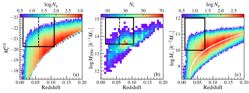
Figure 1: Galaxy and cluster samples selected for our analysis in the paper. Panel (a): Number distribution of SDSS main sample galaxies on the r-band absolute magnitude (K-corrected to $z{=}0.0$) vs. redshift plane, colourcoded by the colourbar on top. Thick black box indicates the luminosity-limited galaxy sample used by our small-scale tidal analysis, split by the vertical dashed line at $z{=}0.06$ into the low- and high-redshift subsamples. Panel (b): Similar to Panel (a), but for the Y07 groups/clusters on the halo mass vs. redshift plane. Panel (c): Similar to Panel (a), but for the stellar mass-limited galaxy sample used by our large-scale tidal analysis. White solid curve indicates the stellar mass threshold above which the SDSS observation is roughly complete.

2 Data

Our analyses in this work are primarily based on the main galaxy sample (Strauss et al., 2002) of the Sloan Digital Sky Survey Data Release 7 (Abazajian et al., 2009). For the parent galaxy sample for bar detection, we construct a luminosity-limited volume-complete sample from the bbright0 sample in the NYU-VAGC catalogue (Blanton et al., 2005), including $131455$ galaxies with redshift $0.01{\leq}z{\leq}0.11$ and r-band absolute magnitude brighter than $M_{\mathrm{r}}^{\mathrm{lim}}{=}{-}20.25$ (K-corrected to $z{=}0$ following Blanton & Roweis (2007)). The values of the maximum redshift $z_{\mathrm{max}}$ and magnitude limit are chosen so that a typical bar in the galaxy with $M_{\mathrm{r}}{\simeq}{-}20.25$, which is around $3\,\mathrm{kpc}$ in length, can be roughly resolved by the SDSS r-band imaging at $z_{\mathrm{max}}$ with a median seeing of 1.32 arc-seconds, which corresponds to $2.7\,\mathrm{kpc}$ at $z{=}0.11$. In addition, the bar size of galaxies brighter than ${-}20.25$ increases rapidly with stellar mass as $M_{*}^{0.6}$ (Erwin, 2019), rendering most of bars detectable in our sample. From the parent luminosity-limited sample, we remove $31010$ highly-inclined discs that are unfit for bar detection by requiring their outer ellipticity $e_{90}{<}0.5$, where $e_{90}$ is defined as the ellipticity of the isophote which encloses $90\%$ of the total luminosity. We measure $e_{90}$ using the isophote fitting described in §4.1. In total, we have $100445$ galaxies that are roughly face-on in the luminosity-limited sample.

When measuring the bar strength in §4, we minimize the contamination from neighbouring galaxies (e.g., when subtracting the 2D disc) by using the r-band SDSS atlas (Stoughton et al., 2002) images downloaded from the SDSS Data Archive Server (DAS). Each atlas image stamp only includes the light originated from the galaxy in the centre of the stamp, therefore providing a clean 2D surface brightness (SB) distribution for ellipse fitting. In order to perform the disc subtraction (see §4.1 for details), we adopt the structural parameters measured by Simard et al. (2011) from the r-band image of each galaxy, including the bulge-to-total ratio ($\mathrm{B}/\mathrm{T}$), the effective radius and position angle (PA) of the bulge, the scale length and PA of the disc, and the inclination angle. The fractional uncertainties in the measurements of the disc inclination and PA are both around $2{-}3\%$, producing robust 2D disc models for the majority of galaxies in our sample. In addition, for the visual validation of our bar detection method, we also present the galaxy images from the DESI DR9 imaging (Dey et al., 2019), which are ${\sim}1.4$ magnitudes deeper than SDSS in the r-band. We plan to directly apply our bar detection method to the DESI imaging data in a follow-up paper (Deng et al. in prep). We construct the color composite SDSS and DESI images for each galaxy using the method described in Lupton et al. (2004).

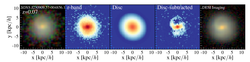
Figure 2: Five different types of images of an example galaxy at $z{=}0.07$, including (from left to right) the SDSS gri colour composite image, original SDSS r-band image, best-fitting 2D disc model, disc-subtracted SDSS r-band image, and the DESI grz colour composite image. The bar-like structure is reasonably recognisable in the DESI image, but is not revealed in the SDSS images until after the disc subtraction.

For the comparison with visual inspection, we make use of the results from the second phase of the Galaxy Zoo (GZ2) project (Willett et al., 2013). As one of the most popular citizen science projects in Astronomy, GZ2 asks volunteers from the public to classify the morphology of SDSS galaxies through a carefully constructed decision tree. In essence, the volunteers were asked to choose an answer to a descriptive question on the galaxy morphology at each step along the decision tree. The fraction of people choosing a particular answer to one question for the galaxy can be interpreted as the probability for the galaxy to have that particular morphological feature. The large number of galaxies with probabilistic visual classifications makes GZ2 one of the most valuable galaxy morphology catalogue to date. For our comparison, we use the consistency-weighted (see section 3.2 of Willett et al., 2013) bar fraction as the probability of a galaxy hosting a bar in GZ2 and denote it as $\mathrm{P_{GZ2}}$. We are aware of the latest GZ2 product using the DESI DECaLS images (Walmsley et al., 2022), which however includes galaxies in a smaller footprint than SDSS and is thus less useful for our comparison.

To identify strong tidal environments on small scales, we select interacting pairs of clusters from the spectroscopic group catalogue of Yang et al. (2007, hereafter referred to as Y07). The Y07 groups were identified by applying an adaptive halo-based group finder to the SDSS main galaxy sample, and we refer interested readers to Yang et al. (2005, 2007) for the technical details. We assume the brightest cluster galaxies (BCGs) as the centres of the clusters, as weak lensing studies showed that the BCGs are generally better centroids than the default luminosity-weighted centres (Wang et al., 2022; Golden-Marx et al., 2022). Y07 provided a halo mass estimate $M_{180m}$ for each group using abundance matching. To facilitate our comparison with the Y19 results, we convert $M_{180m}$ into $M_{200c}$ using the fitting formula from Hu & Kravtsov (2003). We also make sure each selected cluster has at least $5$ spectroscopic member galaxies found by the Y07 catalogue. After selection, our sample includes $1501$ ($600$) clusters with $\log M_{200c}{\geq}13.55$ ($13.85$) between redshift $0.015$ and $0.105$. The redshift range of the cluster sample is slightly narrower than that of the luminosity-limited galaxy sample, thereby providing a complete coverage of the galaxy environment surrounding the clusters at the bin edges. Our selection results in $109$ clusters with mass above $\log M_{200c}{=}13.85$ in the redshift range of $0.015{<}z{<}0.06$, similar to the sample size in the Y19 analysis that included $105$ clusters within the same redshift range. However, by extending the analysis up to $0.105$, we probe a comoving volume that is about six times that of the Y19 analysis, yielding $600$ clusters above $\log M_{200c}{=}13.85$ within our full redshift range of $0.015{<}z{<}0.105$.

For measuring the large-scale tidal anisotropy parameter, we follow the method described by Alam et al. (2019) and select a stellar mass-limited sample with $z\in[0.01,0.074]$ and $\log M_{*}{>}10$ as the tracer of the underlying dark matter density field. For the seven per cent galaxies without redshift due to fibre collision, we assign them the redshifts of their nearest neighbours. To minimize the boundary effect in calculating the tidal field, we only include galaxies within the contiguous area in the North Galactic Cap and those in regions with angular completeness larger than $0.8$. We adopt the stellar mass estimates from the latest MPA-JHU value-added galaxy catalogue, derived following the philosophy of Kauffmann et al. (2003) and Brinchmann et al. (2004) assuming the Chabrier (Chabrier, 2003) initial mass function and the Bruzual & Charlot (2003) stellar population synthesis model. Based on the stellar mass completeness limit estimated in Zu & Mandelbaum (2015), we expect the SDSS main galaxy sample to be roughly volume-complete within $z{=}0.074$ down to $\log M_{*}{=}10$. We choose a lower maximum redshift ($0.074$) than that of the luminosity-limited one ($0.11$), because the tidal anisotropy calculation requires a higher galaxy number density. In total, the stellar mass-limited sample includes $65222$ galaxies.

Figure 1 summarises the samples used by the analyses in the current work, including the luminosity-limited galaxy sample, Y07 cluster sample, and the stellar mass-limited galaxy sample, inside the thick black box shown in the left, middle, and right panel, respectively. In each panel, the 2D histogram indicates the number distribution of all SDSS galaxies (clusters) on the redshift vs. stellar (halo) mass plane, colour-coded by the colourbar on top. For the left and middle panels, each black dashed vertical line indicates the redshift ($0.06$) that we use to split the overall sample into the low- and high-redshift subsamples. The white curve in the right panel indicates the mixture limit derived by Zu & Mandelbaum (2015), above which the galaxy sample should be roughly complete in stellar mass.

3 Measurement of Tidal Density Environments

3.1 Small Scales: Interacting Cluster Pairs

Following Y19, we classify each cluster pair as interacting vs. non-interacting based on their projected physical separation and the line-of-sight velocity difference. In particular, an interacting pair of clusters should have the projected separation $D$ smaller than twice the sum of the two cluster radii $R_{200c}$, and the velocity difference $\Delta v$ smaller than $750\,\mathrm{km}/s$. After applying those criteria, we identify $274$ clusters in interacting pairs among the $1501$ clusters in our overall sample with $\log M_{200c}{\geq}13.55$, and the numbers reduce to $138$ interacting clusters out of the $600$ clusters above $\log M_{200c}{=}13.85$. Splitting the cluster sample above $\log M_{200c}{=}13.55$ ($13.85$) by redshift, we find $47$ ($25$) interacting clusters among the $309$ ($109$) clusters within $z\,{=}[0.015,0.06]$ and $227$ ($113$) interacting out of $1192$ ($491$) within $z\,{=}[0.06,0.105]$. Within the low-redshift bin that overlaps with the Y19 sample, we recover $91$ out of their $105$ clusters and all $16$ of their clusters in interacting pairs.

The membership criteria adopted by the Y07 group finder are relatively stringent. We instead follow the practice of Y19 and re-define the member galaxies associated with each cluster as those projected within $R_{200c}$ from the BCG and have line-of-sight velocities relative to the BCG within $\pm 3\sigma_{v}$, where $\sigma_{v}$ is the line-of-sight velocity dispersion of the cluster so that $\sigma^{2}_{v}=GM_{200c}/(3R_{200c})$. We will adopt this new membership definition for the small-scale tidal analysis in §5.1.

3.2 Large Scales: Tidal Anisotropy Parameter

We quantify the strength of the large-scale tidal field using the tidal anisotropy parameter $\alpha_{R}$, first introduced by Paranjape et al. (2018) as a measure of the anisotropic level of the tidal field. The original definition of $\alpha_{R}$ is

$$\alpha_{R}=\sqrt{q_{R}^{2}}(1+\delta_{R})^{-1},$$ (1)

where $\delta_{R}$ is the spherical overdensity within a sphere of radius r centred on the halo/galaxy and $q_{R}^{2}$ is the tidal shear that can be computed as (Heavens & Peacock, 1988; Catelan & Theuns, 1996)

$$q_{R}^{2}=\frac{1}{2}[(\mathrm{\lambda_{3}}-\mathrm{\lambda_{2}})^{2}+(\mathrm{\lambda_{2}}-\mathrm{\lambda_{1}})^{2}+(\mathrm{\lambda_{3}}-\mathrm{\lambda_{1}})^{2}],$$ (2)

where $\lambda_{1}{<}\lambda_{2}{<}\lambda_{3}$ are the eigenvalues of the tidal tensor. Following Alam et al. (2019), we use a variant of Equation 1 (as will be shown further below) to measure the tidal anisotropy parameter over the galaxy density field smoothed over $5\,h^{-1}\mathrm{Mpc}$ (hereafter referred to as $\alpha_{5}$). We briefly summarize the procedure for calculating $\alpha_{5}$ and refer interested readers to Alam et al. (2019) for the technical details. Firstly, we calculate the density field $\delta$ at each galaxy’s position as the inverse of the volume associated with that galaxy derived using the Voronoi tessellation technique. We then interpolate the density field on a regular Cartesian grid and smooth the density field using a Gaussian kernel of width $5\,h^{-1}\mathrm{Mpc}$ to remove discontinuities near the masked regions or survey boundaries; Secondly, we derive the gravitational potential from the overdensity field by solving the Poisson equation and then compute $q_{5}$ using the components of the tidal tensor derived in the Fourier space; Lastly, we calculate $\alpha_{5}$ via

$$\alpha_{5}=\sqrt{q_{5}^{2}}(1+\delta_{5})^{-0.55},$$ (3)

where we have changed the power-law index from $-1$ in Equation 1 to $-0.55$. As demonstrated by Alam et al. (2019) (see their Fig. 1), using $\alpha_{5}$ defined in this way minimizes the residual correlation between the tidal anisotropy $\alpha_{5}$ and the overdensity $\delta_{8}$, the galaxy overdensity within a sphere of radius $5\,h^{-1}\mathrm{Mpc}$ centred on each galaxy, computed in the same way as $\delta_{5}$ in Equation 3. Therefore, any observed bar dependence on $\alpha_{5}$ in our analysis should in principle be free of contamination from the potential dependence of bars on $\delta_{8}$.

4 Bar Detection Method

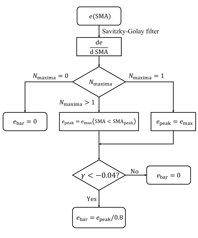
Figure 3: Flowchart of our automated bar detection algorithm based on ellipse fitting. We start from the ellipticity profile $e(\mathrm{SMA})$ measured from the SDSS r-band atlas image either before or after the disc subtraction, and arrive at our bar strength estimate $e_{\mathrm{bar}}$. See text for details.

To robustly characterize the barred galaxy population over a relatively large redshift range ($z{=}0.01-0.11$) using SDSS images, we develop an automated bar detection method based on the ellipse fitting of galaxy isophotes. In particular, to highlight any potential bar-like structure within the co-rotation radius, we subtract the best-fitting 2D model of the disc component from each galaxy image before searching for bars. Compared with the conventional ellipse fitting, our method improves the bar detection accuracy significantly at the high redshift by enhancing the image contrast within the central region against the overall reduction in image quality and spatial resolution.

In the following we describe the ellipse fitting (§4.1), bar identification (§4.2), and compare our bar detection results with the $\mathrm{P_{GZ2}}$ from GZ2 (§4.3), including visual validations using galaxy images from the DESI imaging data. Readers who are only interested in the observational results on the tidal dependence of bars can skip this section to the results in §5.

4.1 Ellipse fitting and disc subtraction

We carry out isophote fitting using the Python implementation (photutils.Ellipse) of the standard iterative ellipse fitting method of Jedrzejewski (1987). We apply the fit twice on the atlas image stamp of each galaxy, first before and then after subtracting the 2D disc component. During each fit, we measure the isophotes at logarithmic intervals of semi-major axis length (SMA), starting from the innermost 1 arc-second radius to two times $R_{90}$, the radius that encloses $90\%$ of the Petrosian flux in r-band. Since each isophote is characterised by its SB level, ellipticity, PA, and SMA, we can obtain two sets of SB, ellipticity, and PA profiles as functions of SMA for each galaxy, one with the disc and the other without.

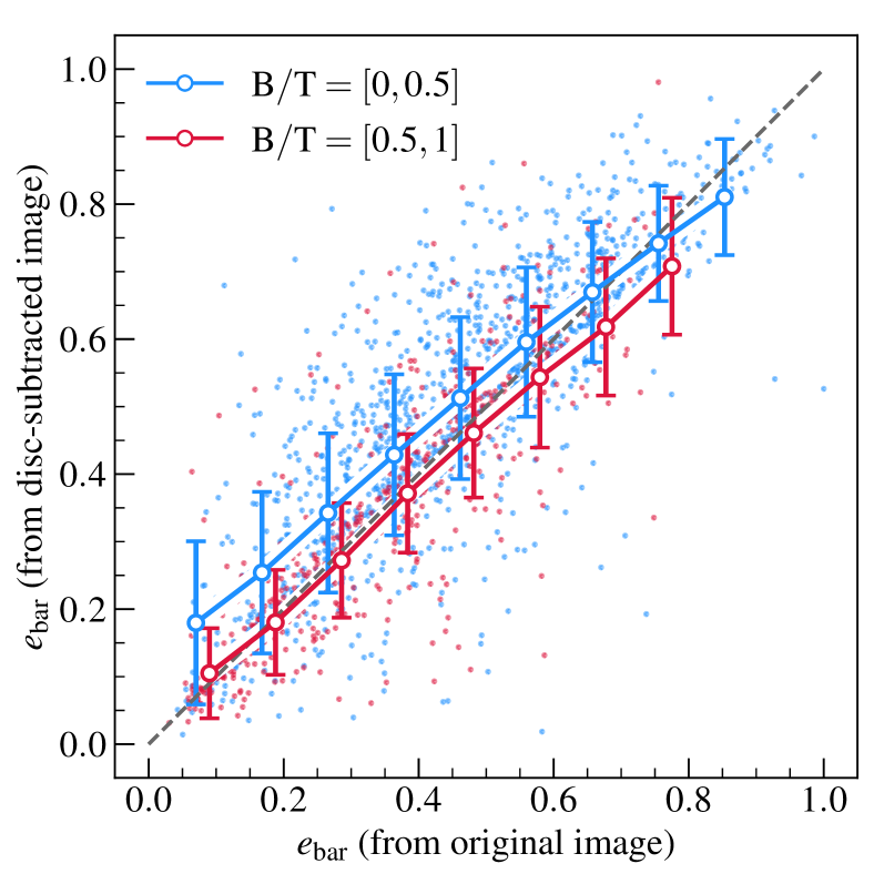
Figure 4: Comparison between the $e_{\mathrm{bar}}$ measurements before (x-axis) and after (y-axis) the disc subtraction. Blue and red dots indicate the measurements of individual galaxies with $\mathrm{B}/\mathrm{T}<0.5$ and $\mathrm{B}/\mathrm{T}\geq 0.5$, respectively. Blue (Red) open circles with errorbars indicate the mean relation with $1{-}\sigma$ scatter for the $\mathrm{B}/\mathrm{T}<0.5$ ($\mathrm{B}/\mathrm{T}\geq 0.5$) populations.

Figure 2 illustrates the efficacy of disc-subtraction in revealing the bar embedded in the bright disc of a face-on galaxy at $z{=}0.07$. From left to right, we show the SDSS gri colour composite image, the SDSS r-band image, the best-fitting 2D disc model of Simard et al. (2011), the SDSS r-band image after subtracting the 2D disc model, and the grz colour composite image from DESI imaging, respectively. The bar barely shows up in the SDSS colour composite and the r-band image, but after the 2D disc model is subtracted, the SDSS r-band image clearly reveals a bar-like structure connected by spiral arms at both ends, which is corroborated by the deeper image from the DESI Legacy Surveys (Dey et al., 2019).

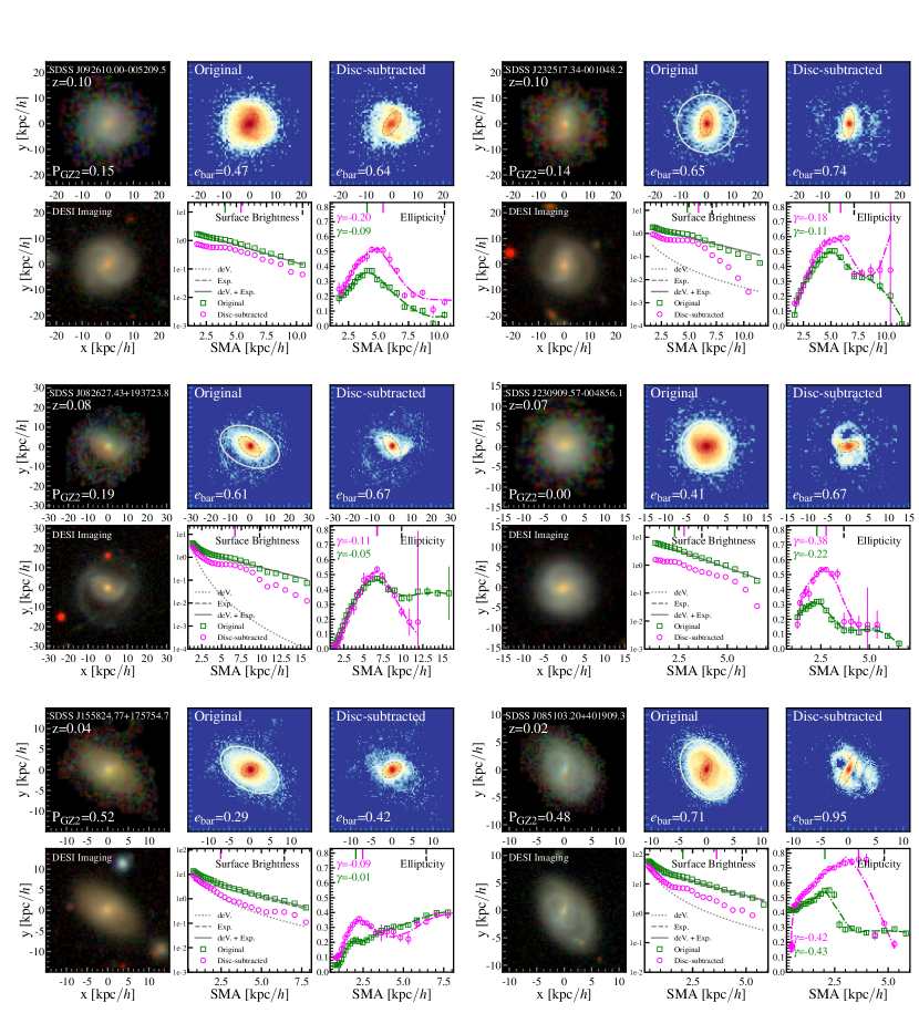
Figure 5: Demonstration of our bar detection method based on the ellipse fitting using six example galaxies, ordered by decreasing redshift (from left and right, top to bottom). For the three-by-two set of panels for each galaxy, the top left panel shows the SDSS gri colour composite image, with the galaxy id and redshift listed in the top left corner and the GZ2-estimated bar probability $\mathrm{P_{GZ2}}$ in the bottom left corner. The bottom left panel shows the DESI grz colour composite image of the same galaxy. The top middle and right panels are the original and disc-subtracted SDSS r-band images, with the measured $e_{\mathrm{bar}}$ labeled in the bottom left corner, respectively. The gray dashed ellipses in both panels indicate the isophote with maximum ellipticity, while the white solid ellipse in the top middle panel marks the isophote that encloses $90\%$ of the total luminosity. The bottom middle and right panels show the surface brightness and the ellipticity profile measured from the original image (green squares) and the disc-subtracted image (magenta circles), respectively. In the bottom middle panel, the solid gray curve is the best-fitting 1D SB model consisting of a de Vaucouleurs (dotted) and an exponential (dashed) profile. In the bottom right panel, the dot-dashed curves are the smoothed ellipticity profile derived from the Savitzky-Golay filter, and the two estimates of the minimum slope $\gamma$ are indicated in legend.

To subtract the 2D disc component of a galaxy, we make use of the best-fitting 1D and 2D SB profiles of the disc component derived by Simard et al. (2011) using a 2D bulge-disc decomposition method. Briefly, we fit a combination of a $\mathrm{S\acute{e}rsic}\,n=4$ bulge and an exponential disc 1D model to the measured SB profile to get the SB amplitude of the disc component. Together with the scale length, inclination angle, and PA of the disc derived by Simard et al. (2011), we build a 2D SB model for the disc and subtract it from the galaxy r-band image. In some cases, we scale down the amplitude of the disc model in order to avoid hitting zero SB in the outskirt of the disc-subtracted image. After the 2D disc component is subtracted, we then re-apply the same isophote fitting method to the disc-subtracted image to obtain our fiducial ellipticity and PA profiles for bar detection.

4.2 Bar identification

We search for the presence of bars based on their distinct imprint on the ellipticity and PA profiles of galaxies. In particular, as a highly elongated structure through the galaxy centre, a bar would induce an increasing trend of the ellipticity profile on small scales, resulting in a prominent peak at ${\sim}1.5{-}10\,\mathrm{kpc}$ (Marinova & Jogee, 2007) that then drops off rapidly as the bar ends at close to the co-rotation radius (e.g., Laine et al., 2002; Jogee et al., 2004; Aguerri et al., 2005; Marinova & Jogee, 2007; Li et al., 2011). Meanwhile in the PA profile, the bar should maintain a relatively constant PA for the isophotes inside the bar region, before transitioning to the PA of the outer disc. For a real stellar bar, the peak ellipticity is closely related to the eccentricity of the periodic orbits in the $x1$ family that underpins the bar, hence providing us a robust measure of the bar strength (Athanassoula, 1992; Martin, 1995; Marinova & Jogee, 2007; Li et al., 2011).

Following the philosophy outlined above, our automated bar detection algorithm is illustrated by the flowchart shown in Figure 3. Given the observed ellipticity profile of a face-on disc galaxy, we calculate its first-order derivative profile $\mathrm{d}e/\mathrm{d}\mathrm{SMA}$ using the Savitzky & Golay filter that accounts for the uncertainties of the ellipticity measurements. We then identify all the $N_{\mathrm{maxima}}$ local maxima between $1.5\,\mathrm{kpc}$ and $\mathrm{SMA}_{90}$ based on the derivative profile. The minimum search radius is chosen to exclude the possible impact from a bulge, while for galaxies with noisy ellipticity profiles we modify the maximum search radius to the SMA where the error in ellipticity exceeds $0.05$ for at least three consecutive isophotes.

If no peaks are found ($N_{\mathrm{maxima}}{=}0$), we identify the galaxy as barless and assign it a zero $e_{\mathrm{peak}}$, and if $N_{\mathrm{maxima}}{=}1$, we assign the ellipticity of that single peak to the galaxy as its $e_{\mathrm{peak}}$. However, in some cases, there are more than one peak and the highest peak usually corresponds to the ellipticity of the outer region rather than the bar. To correctly identify the bar in the inner region, we assign the ellipticity of the secondary peak found within the radius of the highest peak (but still above $1.5\,\mathrm{kpc}$) as the $e_{\mathrm{peak}}$. We mark the location of the peak ellipticity as $\mathrm{SMA}_{\mathrm{peak}}$. After this step, we identify $92814$ out of the $100445$ face-on galaxies as having positive $e_{\mathrm{peak}}$.

Next, we quantify the steepness of the decline following the peak ellipticity using the minimum slope parameter $\gamma$, defined as

$$\gamma=\mathrm{min}\left(\frac{\mathrm{d}\,e}{\mathrm{d}\,\mathrm{SMA}}\right)_{\mathrm{SMA}>\mathrm{SMA}_{\mathrm{peak}}}.$$ (4)

Since $\gamma$ is negative, the absolute value of $\gamma$ is larger when the elongated structure ends more abruptly, hence a higher probability of being a real bar. Some inclined discs or bulge-dominated galaxies may exhibit a peak in the ellipticity profile despite the lack of a bar. In those systems, the peak would slowly give way to the ellipticity of the outer light distribution, rather than experiencing a sharp cutoff. To remove those false positives, we set the peak ellipticity of any galaxy with $\gamma{>}{-}0.04$ to be zero. We have verified that our results are insensitive to the choice of the minimum value of $\gamma$ (at least between ${-}0.08$ and ${-}0.02$). This procedure reclassifies $29312$ out of $92814$ galaxies with positive $e_{\mathrm{peak}}$ into the barless category, with $63502$ galaxies remained possibly barred.

Following Y19, we require the variation of PA to be less than $20^{\circ}$, starting from where the ellipticity first reaches $0.25$ to $\mathrm{SMA}_{\mathrm{peak}}$. The stable PA requirement helps excluding the high ellipticities caused by spurious features such as some tightly wound spiral arms. We do not require a change in the PA profile between the bar and the disc as the disc is subtracted in our fiducial analysis. The PA selection further removes $2009$, leaving $61493$ barred galaxies with $e_{\mathrm{peak}}{>}0$.

Finally, we can measure two types of bar strength for each galaxy using the $e_{\mathrm{peak}}$ measured from the original and disc-subtracted images. For the sake of convenience, we define a new bar ellipticity parameter $e_{\mathrm{bar}}$ by normalising the values of $e_{\mathrm{peak}}$

$$e_{\mathrm{bar}}=\frac{e_{\mathrm{peak}}}{\mathrm{max}(e_{\mathrm{peak}})},$$ (5)

where the denominator is the maximum peak ellipticity, which is $0.8$ in either set of measurements. We will use $e_{\mathrm{bar}}$ to quantify bar strength throughout the rest of the paper.

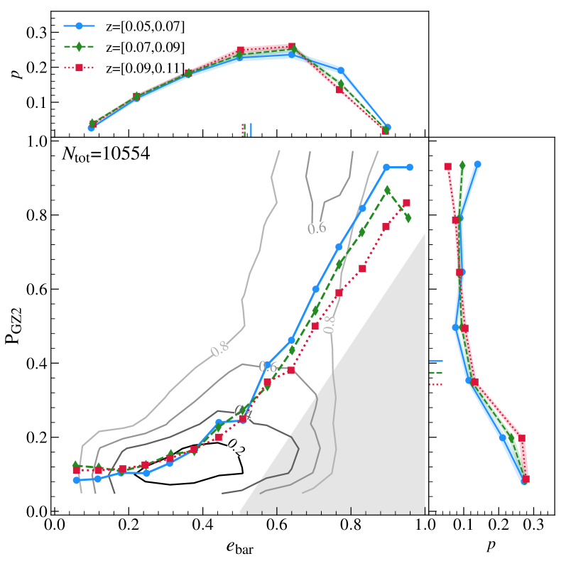
Figure 6: Distribution of barred galaxy candidates (i.e., with both $e_{\mathrm{bar}}{>}0$ and $\mathrm{P_{GZ2}}{>}0$) from the luminosity-limited sample on the $\mathrm{P_{GZ2}}$ versus $e_{\mathrm{bar}}$ plane. In the main panel, the contour levels represent $20\%$, $40\%$, $60\%$, and $80\%$ of the galaxies, with the total number of galaxies listed in the top left corner. The curves of different colours and symbols show the median relationships in three redshift slices (blue solid for $0.05{<}z{<}0.07$, green dashed for $0.07{<}z{<}0.09$ and red dotted for $0.09{<}z{<}0.11$). The shaded triangular region in the bottom right corner highlights the galaxies with strong discrepancies between the two measurements. The two side panels show the 1D probability distributions and the corresponding errors (shaded) of $e_{\mathrm{bar}}$ (top) and $\mathrm{P_{GZ2}}$ (right) for the three redshift slices, colour-coded the same way as in the main panel. The short vertical rungs of matched colours and styles indicate the mean values of the 1D distributions.

Figure 4 compares the two $e_{\mathrm{bar}}$ measurements before and after the disc subtraction, with each blue (red) dot representing a galaxy with $\mathrm{B}/\mathrm{T}{<}0.5$ ($\mathrm{B}/\mathrm{T}{\geq}0.5$). The blue (red) open circles with errorbars indicate the mean relation between the two measurements along with its $1{-}\sigma$ scatter for the $\mathrm{B}/\mathrm{T}{<}0.5$ ($\mathrm{B}/\mathrm{T}{\geq}0.5$) galaxies. As mentioned in the introduction, the measured shape of the bar can be blunted by the light from the disc (Gadotti, 2008), leading to an underestimation of the bar ellipticity or even an undetected bar. Compared with the one-to-one relation (dashed line), the mean relation of the disk-dominated galaxies (blue circles) indicates that after disc subtraction, $e_{\mathrm{bar}}$ generally increases by an amount between $0.1$ and $0.05$ for galaxies with weak bar-like features ($e_{\mathrm{bar}}{<}0.4$), and stays roughly unchanged for galaxies with strong bars ($e_{\mathrm{bar}}{>}0.7$). This behaviour before and after the disc subtraction is consistent with our expectation that the disc subtraction helps mitigating the impact from bright discs in weakly-barred systems. Meanwhile, the mean relation of the bulge-dominated galaxies (red circles) indicates that the two measurements are roughly consistent for most of the galaxies, but exhibit a slight decrease in $e_{\mathrm{bar}}$ after the disc subtraction for those with $e_{\mathrm{bar}}{>}0.7$. Since many of the high-$e_{\mathrm{bar}}$, high-$\mathrm{B}/\mathrm{T}$ systems are false positives, the decrease is probably caused by the fact that the bulge component becomes less bar-like after the disk removal, hence an improvement of the method. In addition, we have performed a suite of mock tests of the impact of inaccurate 2D disc models on the bar strength, and find that the number of false positives caused by the small uncertainties associated with the Simard et al. (2011) disc models is negligible in our paper. As a result, we adopt the $e_{\mathrm{peak}}$ measured from the disc-subtracted SB profiles as our fiducial peak ellipticity estimates.

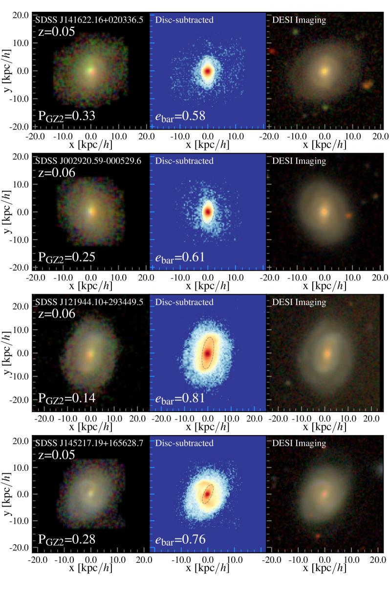
Figure 7: Examples of four galaxies with high $e_{\mathrm{bar}}$ but low $\mathrm{P_{GZ2}}$. In each row, the left panel shows the SDSS gri colour composite image of the galaxy, with $\mathrm{P_{GZ2}}$ listed in the lower left corner. The middle panel shows the disc-subtracted SDSS r-band image along with the ellipse with maximum ellipticity (gray dashed) and the measured $e_{\mathrm{bar}}$ value in the lower left. For comparison, the right panel shows the DESI grz colour composite image of the same galaxy.

Figure 5 demonstrates the efficacy of our bar detection method based on the ellipse fitting of disc-subtracted images of six candidate barred galaxies, ordered by decreasing redshift (from left and right, top to bottom). For the three-by-two panels of each galaxy, the top left panel is the SDSS gri colour composite image, with the galaxy id and redshift listed in the top left corner and the GZ2-estimated bar probability $\mathrm{P_{GZ2}}$ in the bottom left corner. The top middle and top right panels display the original and disc-subtracted SDSS r-band images of the galaxy, respectively. In each of the two panels, the dashed gray ellipse indicates the isophote with maximum ellipticity, which corresponds to the location of the candidate bar ($e_{\mathrm{bar}}$ value listed in the bottom left corner). The solid white ellipse in the top middle panel indicates the isophote that encloses $90\%$ of the total luminosity, hence with ellipticity $e_{\mathrm{90}}$. The bottom left panel displays the DESI grz colour composite image of the same galaxy, from which we can better evaluate the ellipticity and PA of the bar-like structure visually. The bottom middle and right panels show the SB and ellipticity profiles, respectively. In the bottom middle panel, the green squares with errorbars are the 1D SB profile measured from the original SDSS r-band image shown in the top middle panel. The gray solid curve indicates the best-fitting 1D SB model from Simard et al. (2011) to the green squares, consisting of a de Vaucouleurs component (dotted) and an exponential disc profile (dashed). The magenta squares with errorbars indicate the 1D SB profile measured from the disc-subtracted r-band image shown in the top right panel. The bottom right panel compares the ellipticity profile measured from the disc-subtracted image (magenta circles with errorbars) to that from the original image (green squares with errorbars), each fitted with a smooth model (dot-dashed curves) derived from the Savitzky-Golay filter. The two estimates of the minimum slopes are also listed in the top left corner.

In the first four cases shown in Figure 5, the visual evidence of a bar presence in the SDSS images is rather weak, consistent with the low $\mathrm{P_{GZ2}}$ values given by GZ2 (below $0.2$). However, the DESI images generally reveal a much stronger bar-like structure in the centre than the SDSS images, suggesting that the lack of visual detections in GZ2 is due to the fact that those four galaxies are relatively distant with redshifts $z{>}0.07$. Using the SDSS original r-band images, our ellipse fitting method successfully identifies an elongated structure in each galaxy, with $e_{\mathrm{bar}}$ values ranging from $0.41$ to $0.65$ (thick green ellipses), but the PAs of the ellipses are generally offset from the actual bar shown in the DESI images by $5{-}15$ degrees. Such a PA offset is not limited to the four high-redshift galaxies, but exists even in the bottom row where the two galaxies are relatively nearby with redshifts below $0.04$, signaling a bias in the $e_{\mathrm{bar}}$ derived using the original SDSS images regardless of redshift.

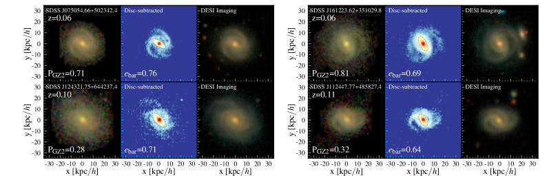
Figure 8: Two pairs of "twins" galaxies that have similar physical and morphological properties but observed at different redshifts. For each pair in the same column, the top row shows the standard three-panel view (same format as in Figure 7) of the galaxy at the lower redshift, while the bottom row shows its "twin" at the higher redshift. While the $e_{\mathrm{bar}}$ and $\mathrm{P_{GZ2}}$ measurements agree well at the low redshifts, they tend to differ significantly at the higher redshifts.

The PA offset problem is significantly alleviated in our fiducial bar detection method using disc-subtracted images, suggesting the bar morphologies are better approximated by the highest-$e_{\mathrm{peak}}$ ellipses in our fiducial measurements. As a result, the ellipticity profiles are generally more strongly peaked after disc subtraction compared to the original ones, yielding increases in $e_{\mathrm{bar}}$ ranging between $\Delta e_{\mathrm{bar}}{=}0.05$ and $0.23$. In addition, the minimum slope $\gamma$ generally drops after disc subtraction (except for the nearest object), illustrated by the strong discontinuities in the ellipticity profiles (magenta circles) following the occurrences of peak ellipticities.

4.3 Comparison with Visual Bar Identifications

We now quantitatively compare the bar strengths $e_{\mathrm{bar}}$ calculated by our fiducial bar detection method with the bar probabilities $\mathrm{P_{GZ2}}$ derived by the state-of-the-art visual identifications from the GZ2 catalogue. To avoid any discrepancies caused by small number statistics in the visual inspection, we limit our comparison to galaxies that have received more than five responses to “whether the galaxy is barred” by the citizen scientists in GZ2. In total, we have $20979$ face-on galaxies between $0.05{<}z{<}0.11$ with robust measurements of both $e_{\mathrm{bar}}$ and $\mathrm{P_{GZ2}}$. Among those, $10554$ of them are measured with both $e_{\mathrm{bar}}{>}0$ and $\mathrm{P_{GZ2}}{>}0$, $4117$ with $e_{\mathrm{bar}}{=}0$ but $\mathrm{P_{GZ2}}{>}0$, and $2733$ with $e_{\mathrm{bar}}{>}0$ but $\mathrm{P_{GZ2}}{=}0$. By carefully examining the DESI images of those galaxies in the latter two categories, we find that the success rate of either bar detection method is close to $50\%$, suggesting the two methods are comparable in identifying the truly barless galaxies. Below we will focus on the $10554$ galaxies with both positive values of $e_{\mathrm{bar}}$ and $\mathrm{P_{GZ2}}$, as many of them are likely truly barred galaxies that are suitable for comparing the two types of bar strength estimates.

Figure 6 compares the overall 2D distribution (contours) and median relationships in three different redshift bins (blue solid: $0.05{<}z{<}0.07$; green dashed: $0.07{<}z{<}0.09$; red dotted: $0.09{<}z{<}0.11$) on the $e_{\mathrm{bar}}$ vs. $\mathrm{P_{GZ2}}$ plane in the main panel, with their respective 1D distributions in three redshift bins shown in the two side panels. Overall, there exists a good correlation between $\mathrm{P_{GZ2}}$ and $e_{\mathrm{bar}}$ with a Pearson cross-correlation coefficient of $0.57$, indicating a reasonable agreement between the GZ2 visual inspection and our ellipse fitting methods. However, the median $\mathrm{P_{GZ2}}$ as a function of $e_{\mathrm{bar}}$ at fixed redshift is not a diagonal one-to-one relation, but appears flat at $e_{\mathrm{bar}}{<}0.4$ before rising steeply at $e_{\mathrm{bar}}{\geq}0.4$. The flattening is associated with the large number of low-$\mathrm{P_{GZ2}}$ galaxies clustered below $\mathrm{P_{GZ2}}{=}0.3$, as shown by the 1D PDFs of $\mathrm{P_{GZ2}}$ in right panel. Despite being confined within $\mathrm{P_{GZ2}}{=}0.3$, those low-$\mathrm{P_{GZ2}}$ galaxies have a wide spread in $e_{\mathrm{bar}}$, with a good portion of them identified as strongly barred ($e_{\mathrm{bar}}{\sim}0.8$) by our method. The slope of the median relationship at the high-$e_{\mathrm{bar}}$ end evolves significantly with redshift, largely due to the decrease of high-$\mathrm{P_{GZ2}}$ galaxies with increasing redshift (right panel). Meanwhile, the 1D PDF of $e_{\mathrm{bar}}$ is approximately redshift-independent, exhibiting a single broad peak at $e_{\mathrm{bar}}{\sim}0.6$. Therefore, assuming that the redshift evolution of the bar fraction is negligible across the narrow redshift range, Figure 6 suggests that the $e_{\mathrm{bar}}$ estimates are relatively insensitive to the decrease of both the signal-to-noise and physical resolution of the galaxy images with redshift.

To investigate the origin of discrepancies between the two methods, we select all the $1213$ galaxies from the high-$e_{\mathrm{bar}}$, low-$\mathrm{P_{GZ2}}$ corner in Figure 6 (shaded triangular region) and visually compare their corresponding SDSS vs. DESI images. Unsurprisingly, the SDSS images of these galaxies barely exhibit any signatures of bars, but their DESI images tell a very different story — at least $52\%$ of these galaxies are strongly barred based on the DESI images and another $34\%$ of them are likely barred with oval distortions in the centre. Figure 7 shows four examples of such high-$e_{\mathrm{bar}}$, low-$\mathrm{P_{GZ2}}$ galaxies from the lowest redshift bin ($0.05{<}z{<}0.07$), where the physical resolutions of SDSS and DESI images should both be adequate for resolving the strong bars. The four galaxies show little signature of having a bar in the SDSS images (left column), but appear strongly barred based on the values of $e_{\mathrm{bar}}$ (middle column) and the DESI images (right column). The formats of individual panels in each row are the same as the respective panels in Figure 5. In general, the discs of these galaxies are relatively bright, rendering the bar less prominent in the SDSS images; Our ellipse fitting over the disc-subtracted images is able to identify the correct ellipses (gray dashed ellipses) that match the shape and extent of the bars seen in the DESI images very well.

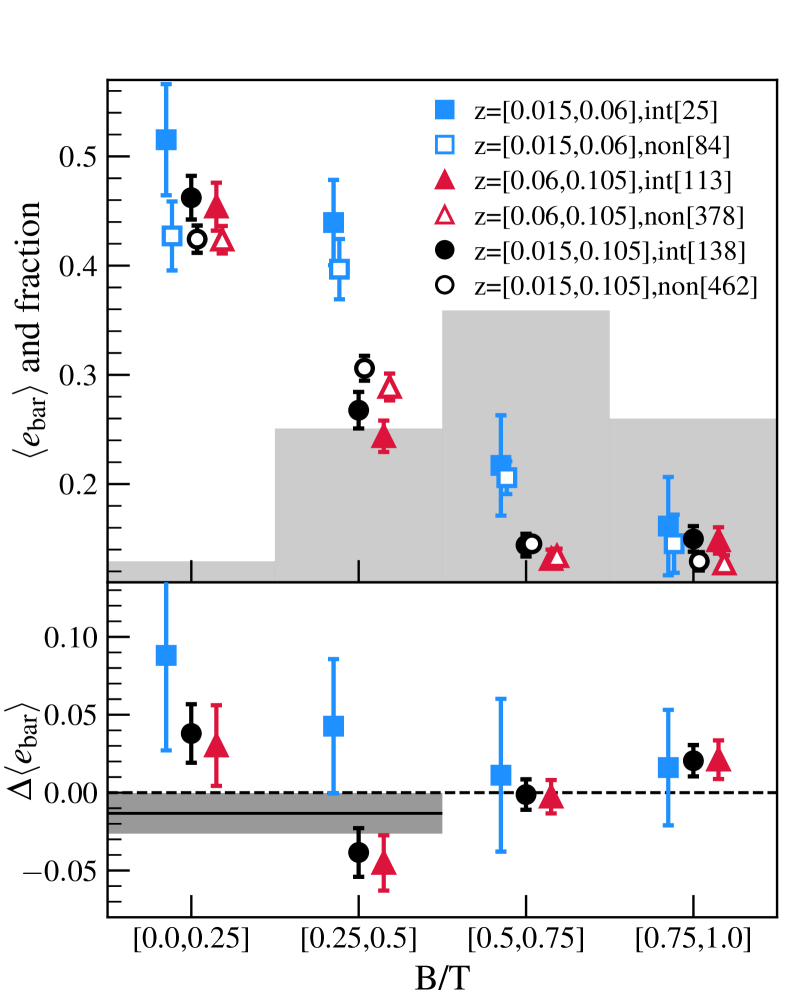
Figure 9: The mean bar strength $\langle e_{\mathrm{bar}}\rangle$ of member galaxies with different $\mathrm{B}/\mathrm{T}$ in interacting (solid symbols) vs. non-interacting clusters (open symbols), while the differences in their $\langle e_{\mathrm{bar}}\rangle$ between interacting and non-interacting clusters are shown in the bottom sub-panel. Blue squares, red triangles, and black circles are for the low-redshift ($0.015{<}z{<}0.06$), high-redshift ($0.06{<}z{<}0.105$), and the full-redshift range cluster samples, respectively, with the numbers of different type of clusters in each redshift bin listed in the legend. The light-shaded histogram in the top panel indicates the relative abundance of member galaxies in the four different $\mathrm{B}/\mathrm{T}$ bins. The black horizontal band in the bottom panel ($\Delta\langle e_{\mathrm{bar}}\rangle{=}{-}0.013{\pm}0.013$) indicates the overall discrepancy between interacting and non-interacting clusters for galaxies with $0{<}\mathrm{B}/\mathrm{T}{<}0.5$. All the errorbars are the $1-\sigma$ uncertainties estimated from Jackknife resampling.

Using the disc-subtracted galaxy images, our automated bar detection method is relatively insensitive to the image quality and physical resolution, as demonstrated by the lack of redshift evolution in the 1D PDFs of $e_{\mathrm{bar}}$ in the top panel of Figure 6. This is very encouraging, showing that it is viable to extend the SDSS analysis of tidal dependence of bars from the local Universe at $z{<}0.06$ (as was done in Y19) to a much larger volume up to $z{=}0.11$ with five times more galaxy clusters. Figure 8 further illustrates the robustness of our fiducial method against redshift with two pairs of barred galaxies. For each pair in the same column, the top row shows the standard three-panel view (same format as in Figure 7) of one galaxy at a lower redshift, which can be compared to the bottom row in which we show the same view of its “twin” galaxy with very similar physical properties (r-band luminosity and effective radius) and appearance (morphology and inclination angle based on the DESI images) but at a higher redshift. For the two galaxies at $z{=}0.06$ (top row), both the GZ2 and our ellipse fitting method regard them as strongly barred, with $\mathrm{P_{GZ2}}{=}(0.71,0.81)$ and $e_{\mathrm{bar}}{=}(0.76,0.81)$, respectively. As expected, the SDSS image quality decreases considerably at $z{\geq}0.10$, resulting in much lower values of $\mathrm{P_{GZ2}}$ for the two “twin” galaxies in the bottom row ($\mathrm{P_{GZ2}}{=}0.28,0.32$). However, our bar detection method yields $e_{\mathrm{bar}}$ values ($e_{\mathrm{bar}}{=}0.71,0.64$) that are consistent with their low-$z$ counterparts ($e_{\mathrm{bar}}{=}0.76,0.69$), confirming our expectation based on the DESI images.

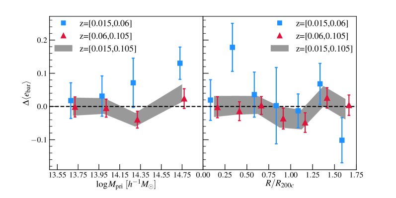
Figure 10: The dependence of $\Delta\langle e_{\mathrm{bar}}\rangle$ on the mass of the primary cluster $M_{\mathrm{pri}}$ (left panel) and the projected cluster-centric distance scaled by the halo radius, $R/R_{200c}$ (right panel). Blue squares and red triangles are for the low ($0.015{<}z{<}0.06$) and high ($0.06{<}z{<}0.105$) redshift subsamples, respectively. The dark shaded bands are the final results from the overall cluster sample. All errorbars are $1{-}\sigma$ uncertainties estimated from Jackknife resampling.

To summarise, our fiducial bar detection method based on the ellipse fitting, when applied to the SDSS r-band images of galaxies with their disc components subtracted, is capable of providing robust measurements of the bar strength parameter $e_{\mathrm{bar}}$. Overall, our method is largely consistent with the visual identification results like the GZ2 at the low redshifts. At higher redshifts, our fiducial bar detection remains robust against the reduction of image quality with redshift at least up to $z{=}0.11$, the maximum redshift of our analysis in the next section.

5 Tidal Dependence of Bars

Equipped with a robust bar detection method, we are now ready to examine the dependence of bar strength, characterised by $e_{\mathrm{bar}}$, on the different tidal environments measured in §3. In particular, we examine the tidal dependence of bar strength $e_{\mathrm{bar}}$ on cluster scales up to three times the virial radius in §5.1, and then shift our focus to the tidal anisotropy field defined over $5\,h^{-1}\mathrm{Mpc}$ scales (measured by $\alpha_{5}$) in §5.2. Theoretically, we expect the small and/or large-scale tidal density fields to both correlate with halo spin, so that any potential tidal dependence of bars may be an indirect evidence of bar dependence on halo spin. In practice, however, our investigation is an agnostic probe of tidal dependence of bars regardless of the physical origin.

5.1 Bar Dependence on the Cluster-scale Tidal Environment

5.1.1 Is There a Boost in the Bar Strength Surrounding Interacting Clusters?

For characterising the cluster-scale tidal environment, we follow the approach of Y19 in §3.1 and split the Y07 cluster sample into two subsamples of interacting vs. non-interacting clusters. The strong tidal forces generated during cluster-cluster interactions could induce ordered shear flows and spin up haloes in the vicinity of the interacting pairs, potentially leaving an imprint on the galactic bars. Recently, Y19 claimed the detection of such a signal by comparing the barred fraction between galaxies in the interacting and non-interacting clusters, but within a relatively short redshift range of $0.015{<}z{<}0.06$. Among the $105$ clusters in their sample, they found a statistically significant enhancement of galaxy bar fraction surrounding the $16$ interacting clusters compared to the $89$ isolated ones.

Compared to the Y19 analysis, our study is different in four major aspects. Firstly, although the two bar detection methods are both based on ellipse fitting, our method measures the bar strength $e_{\mathrm{bar}}$ using the disc-subtracted images of galaxies; Secondly, instead of using the bar fraction based on a binary classification, we compute the average bar strength $\langle e_{\mathrm{bar}}\rangle$ of galaxies in different tidal environments, without resorting to an arbitrary $e_{\mathrm{bar}}$ for dividing barred vs. non-barred galaxies; Thirdly, our measurement uncertainties are computed using the Jackknife resampling technique. Briefly, for each cluster sample with $N$ pairs of interacting clusters, we construct $N$ Jackknife subsamples by removing one pair of interacting clusters and $1/N$ of the isolating systems at a time, and estimate the uncertainty on $\langle e_{\mathrm{bar}}\rangle$ as the standard deviation of the $N$ Jackknife measurements multiplied by $\sqrt{N-1}$. Finally and most importantly, we use the Y07 halo-based group catalogue and extend the maximum redshift of investigation to $z{=}0.11$, resulting in a factor of five increase in the survey volume. In particular, while the size of our cluster sample ($109$ above $\log M_{200c}{=}13.85$) is similar to that of Y19 ($105$) at $0.015{<}z{<}0.06$, our analysis includes $491$ more clusters with $\log M_{200c}{>}13.85$ at $0.06{<}z{<}0.105$, thereby increasing the sample size by a factor of five compared to Y19.

Figure 9 compares the mean $e_{\mathrm{bar}}$ of galaxies between the interacting (filled symbols) and non-interacting clusters (open symbols) in four different bins of bulge-to-total ratio $\mathrm{B}/\mathrm{T}$. In the top panel, blue squares and red triangles show the measurements for the clusters in the low ($0.015{<}z{<}0.06$) and high ($0.06{<}z{<}0.105$) redshift bins, respectively, and the combined results from the full cluster sample are shown by the black symbols. The underlying light-shaded histograms indicate the relative abundance of galaxies in the four different $\mathrm{B}/\mathrm{T}$ bins. Filled symbols of the matching colours and styles in the bottom panel indicate the average difference between the bar strength of galaxies around the interacting and non-interacting clusters, defined as

$$\Delta\langle e_{\mathrm{bar}}\rangle\equiv\langle e_{\mathrm{bar}}^{\mathrm{int}}\rangle-\langle e_{\mathrm{bar}}^{\mathrm{non}}\rangle.$$ (6)

All the errorbars are the $1-\sigma$ uncertainties estimated from Jackknife resampling. As expected, the disc-dominated galaxies ($\mathrm{B}/\mathrm{T}{<}0.5$) are more likely to have strong bars than the bulge-dominated systems ($\mathrm{B}/\mathrm{T}{\geq}0.5$) regardless of redshift or tidal environments. The average bar strength of galaxies with $0.25{<}\mathrm{B}/\mathrm{T}{<}0.75$ is significantly higher in the low redshift bin than in the high redshift one, echoing the finding in Figure 6 where the fraction of high-$e_{\mathrm{bar}}$ galaxies is enhanced at the low redshift.

Comparing the average bar strengths between galaxies in the interacting vs. non-interacting clusters in the low redshift bin, we confirm the results from Y19, finding that the $\langle e_{\mathrm{bar}}\rangle$ of disc-dominated galaxies with $0{<}\mathrm{B}/\mathrm{T}{<}0.25$ ($0.25{<}\mathrm{B}/\mathrm{T}{<}0.5$) surrounding the interacting clusters is $0.088{\pm}0.061$ ($0.043{\pm}0.043$) higher than that around the isolated clusters (blue filled squares in the bottom panel of Figure 9). The discrepancy is consistent with zero for bulge-dominated galaxies with $\mathrm{B}/\mathrm{T}{\geq}0.5$. We note that the volume covered by our low redshift bin overlaps completely with that analyzed by Y19, yielding $91$ clusters in common between the two analyses. Therefore, it is reassuring and unsurprising that the two sets of measurements at $0.015{<}z{<}0.06$ are consistent with each other, despite the differences in methodologies.

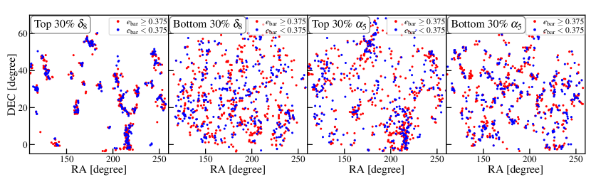
Figure 11: The spatial distribution of more-likely barred galaxies ($e_{\mathrm{bar}}{\geq}0.375$, red) and less-likely barred galaxies ($e_{\mathrm{bar}}{<}0.375$, blue) in the top/bottom $30\%$ of $\delta_{8}$ (left two panels) and $\alpha_{5}$ (right two panels) within a redshift slice of $\Delta z{=}0.007$ centred at $z{=}0.057$.

However, the discrepancy observed for the disc-dominated galaxies becomes significantly weaker in the high-redshift bin where our statistical uncertainties are $2{-}3$ times smaller (red filled triangles in the bottom panel of Figure 9). Intriguingly, $\Delta\langle e_{\mathrm{bar}}\rangle$ remains somewhat positive ($\Delta\langle e_{\mathrm{bar}}\rangle{=}0.030{\pm}0.026$) for the pure discs with $0{<}\mathrm{B}/\mathrm{T}{<}0.25$, but becomes negative ($\Delta\langle e_{\mathrm{bar}}\rangle{=}{-}0.045{\pm}0.018$) for the disc galaxies with $0.25{<}\mathrm{B}/\mathrm{T}{<}0.5$. The discrepancy for the bulge-dominated galaxies ($\mathrm{B}/\mathrm{T}>0.5$) remains largely consistent with zero in the high-redshift bin. Combining the two redshift bins, the overall discrepancy between the interacting vs. non-interacting clusters for galaxies with $0{<}\mathrm{B}/\mathrm{T}{<}0.5$ is $\Delta\langle e_{\mathrm{bar}}\rangle{=}{-}0.013{\pm}0.013$ (gray horizontal band in the bottom panel of Figure 9). Therefore, our analysis over the full redshift range $0.06{<}z{<}0.105$ does not provide any evidence for the enhancement of average bar strength surrounding the interacting clusters compared to the isolated systems.

Focusing on the disc-dominated galaxies with $0<\mathrm{B}/\mathrm{T}<0.5$, we explore whether their $\langle e_{\mathrm{bar}}\rangle$ discrepancy (or lack thereof) between interacting vs. non-interacting clusters depends on the cluster mass or their projected clustercentric distance in Figure 10. The left panel of Figure 10 shows the dependence of $\Delta\langle e_{\mathrm{bar}}\rangle$ on the halo mass of the primary cluster $M_{\mathrm{pri}}$ of the interacting pair. We control the halo mass of the non-interacting clusters to be the same at each fixed $M_{\mathrm{pri}}$ bin, so that any potential discrepancy should be caused by the presence of a massive neighbour. In the low redshift bin (blue filled squares), although $\Delta\langle e_{\mathrm{bar}}\rangle$ increases monotonically with $M_{\mathrm{pri}}$, it is consistent with zero except for in the highest halo mass bin $\log M_{\mathrm{pri}}{>}14.55$ where only nine interacting clusters are found. For galaxies in the high redshift bin (red filled triangles), the monotonic trend disappears and we do not detect any evidence of positive $\Delta\langle e_{\mathrm{bar}}\rangle$ across the entire halo mass range. As a result, the overall $\Delta\langle e_{\mathrm{bar}}\rangle$ from combining the two redshift bins (gray shaded band) is largely consistent with zero at any fixed $M_{\mathrm{pri}}$, implying little to no impact of cluster-scale tidal field on the bar strength. Similarly, the right panel of Figure 10 shows the dependence of $\Delta\langle e_{\mathrm{bar}}\rangle$ on the projected cluster-centric distance scaled by the halo radius, $R/R_{200c}$. Galaxies in the low redshift bin (blue filled squares) exhibit a strong enhancement in $\langle e_{\mathrm{bar}}\rangle$ surrounding the interacting clusters at $0.25{<}R/R_{200c}{<}0.5$, i.e., well within the virialised region of clusters. However, this tantalizing signal of a positive $\Delta\langle e_{\mathrm{bar}}\rangle$ disappears beyond $R=R_{200c}$ (i.e., in the infall region outside the cluster radius) at $0.015{<}z{<}0.06$ and across the entire range of $R/R_{200c}$ at $0.06{<}z{<}0.105$ (red filled triangles). Consequently, the overall signal for galaxies at $0.015{<}z{<}0.105$ (gray shaded band) is consistent with zero between the cluster centre and the infall region, exhibiting no signal of tidal enhancement of bars.

5.1.2 On the Discrepancy between the Observations at Low and High Redshifts

In §5.1.1, at $z<0.06$ we observe the enhanced average bar strength in the vicinity of interacting clusters compared to the isolated systems, as was firstly detected by Y19, but no such signal for the larger sample at $z\geq 0.06$. This difference in the tidal behaviour of bars at the low and high redshifts is intriguing, as it requires a strong evolution in the formation timescale of tidally-induced bars between $z\sim 0.1$ and today (i.e., $\sim 1\,\mathrm{Gyr}$). Since the disc fraction does not vary since $z\sim 0.1$ (van der Kruit & Freeman, 2011), for such a strong evolution in tidal bars to occur, the average bar formation timescale has to decrease dramatically to well below $1\,\mathrm{Gyr}$. Simulations generally predict that the formation timescale of bars depends exponentially on the disc-to-total mass ratio $f_{\mathrm{disc}}$ (Fujii et al., 2018), reaching below $1\,\mathrm{Gyr}$ for galaxies with $f_{\mathrm{disc}}>0.5$. However, a rapid onset of bars due to a boosted $f_{\mathrm{disc}}$ in strong tidal fields is highly unlikely below $z\sim 0.1$, but only plausible in the very high-redshift Universe (Bland-Hawthorn et al., 2023).

Therefore, the discrepancy between the two redshift bins is more likely caused by observational uncertainties. For instance, the efficacy of our bar detection method could diminish rapidly with redshift, thereby smearing the signal that otherwise exists in the high redshift bin. This explanation is plausible, but we have conducted comprehensive tests on the sensitivity of our bar detection method to redshift in §4, which demonstrate that we can distinguish between the barred vs. unbarred galaxies reasonably well up to $z{=}0.11$. In addition, the comparison between galaxies in the interacting vs. non-interacting clusters is done at fixed redshifts, so that any systematic trend of $e_{\mathrm{bar}}$ with redshift would not affect our results. Therefore, our analysis should be able to pick up at least some of the signal within $0.06{<}z{<}0.11$ should it be as strong as was detected at $z{<}0.06$, especially given the significant reduction in the statistical uncertainties due to the much larger cluster sample.

Alternatively, the discrepant results could be simply due to a statistic fluke in the local Universe below $z{=}0.06$, where the observed enhancement of bar strength is primarily contributed by the five cluster pairs (nine clusters in total). In the follow-up paper, we will apply our bar detection method to the DESI images of those galaxies, and investigate if the discrepancy remains (hence more likely a fluke) or could be resolved by the deeper imaging data.

To briefly summarise our results in the current section, we confirm the findings from Y19 and detect an enhancement of the bar strength surrounding interacting clusters at $0.015{<}z{<}0.06$ using our automated bar detection method and the Y07 cluster sample. Furthermore, we find that the enhancement primarily originates from the boosted fraction of barred galaxies within the central region ($R{<}0.5R_{200c}$) of the most massive cluster-cluster pairs ($\log M_{200c}{>}14.55$). However, the enhancement seen in the local clusters below $z{=}0.06$ disappears as more clusters (and their associated galaxies) from the higher redshift up to $z{=}0.11$ are included in our final analysis.

5.2 Barred galaxies in the large-scale tidal environment

We now explore the possible connection between bar strength and tidal environment on the larger scales, where linear theory predicts a correlation between the tidal anisotropy and halo spin, a potential facilitator of bar growth. For the analysis in this section, we switch to the stellar mass-limited ($\log M_{*}>10$) galaxy sample that is volume-complete within $z=[0.01,0.074]$ in §2 and estimate the bar strength of each disc-dominated galaxy ($0{<}\mathrm{B}/\mathrm{T}{<}0.5$) using our automated bar detection method. Following Alam et al. (2019), we measure the spherical galaxy overdensity $\delta_{8}$ as well as the tidal anisotropy parameter $\alpha_{5}$ surrounding each disc-dominated galaxy from the 3D distribution of all galaxies in this sample, as described in §3.2. In addition, Alam et al. (2019) showed that there is no correlation between $\delta_{8}$ and $\alpha_{5}$ (see their Fig. 1), which we have verified explicitly using our sample.

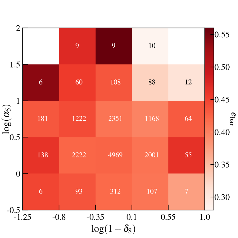
Figure 12: The average bar strength $e_{\mathrm{bar}}$ of galaxies on the $\log(1+\delta_{8})$ vs. $\log\alpha_{5}$ plane, colour-coded by the colour bar on the right. The number in each cell indicates the number of galaxies within that 2D bin.

Figure 11 provides a visually-appealing overview of the different types of environments defined by $\delta_{8}$ or $\alpha_{5}$, showing the spatial distribution of disc-dominated galaxies with $e_{\mathrm{bar}}\geq 0.375$ (red) and $e_{\mathrm{bar}}<0.375$ (blue) in the top/bottom $30\%$ of $\delta_{8}$ (left two panels) and $\alpha_{5}$ (right two panels). To avoid clutter, we only select galaxies from a thin redshift slice of $0.0535{<}z{<}0.0605$. As expected, galaxies in the high- and low-$\delta_{8}$ environments are densely and loosely clustered, respectively, displaying drastically different levels of clumpiness. Meanwhile, galaxy distributions in the high- and low-$\alpha_{5}$ environments have the similar clumpiness, but exhibit markedly different levels of anisotropies on scales larger than ${\sim}10\,h^{-1}\mathrm{Mpc}$. Visually, there is no discernible evidence of segregation between the more-barred vs. less-barred galaxies in any of the four types of environments — any tidal dependence of bars, if exists, must be subtle and thus requires a more quantitative investigation.

We start our investigation with Figure 12, which shows the average bar strength $\langle e_{\mathrm{bar}}\rangle$ of disc-dominated galaxies as a 2D function of $\log(1+\delta_{8})$ and $\log\alpha_{5}$, $\langle e_{\mathrm{bar}}|\alpha_{5},\delta_{8}\rangle$, colour-coded by the colourbar on the right. The number listed within each cell indicates the number of galaxies within that 2D bin of fixed $\delta_{8}$ and $\alpha_{5}$. Overall, we observe a weak trend of declining $\langle e_{\mathrm{bar}}\rangle$ with $\log(1+\delta_{8})$ in the horizontal direction, but a complex trend with $\log\alpha_{5}$ in the vertical direction, especially at $\log\alpha_{5}>1$. The declining trend of $\langle e_{\mathrm{bar}}\rangle$ with $\delta_{8}$ is presented more clearly in Figure 13, where the filled circles (open squares) with errorbars show the dependence of $\langle e_{\mathrm{bar}}\rangle$ ($\mathrm{B}/\mathrm{T}$) of galaxies on $\log(1+\delta_{8})$ using the left (right) y-axis. The declining trend of $\langle e_{\mathrm{bar}}\rangle$ with $\log(1+\delta_{8})$ can be described by a simple linear relation as

$$\langle e_{\mathrm{bar}}|\delta_{8}\rangle=-0.036\log(1+\delta_{8})+0.409,$$ (7)

which is indicated by the black dashed line in Figure 13. This declining trend is likely caused by the strong anti-correlation between $e_{\mathrm{bar}}$ and $\mathrm{B}/\mathrm{T}$, and since the $\mathrm{B}/\mathrm{T}$ of galaxies is higher in denser environments (open squares), it is unsurprising that the average bar strength decreases with increasing $\delta_{8}$. This is consistent with the previous studies that found no significant difference in terms of the local density environment between barred and unbarred galaxies when other physical properties of galaxies (e.g., $\mathrm{B}/\mathrm{T}$) are controlled (Aguerri et al., 2009; Li et al., 2009; Lee et al., 2012).

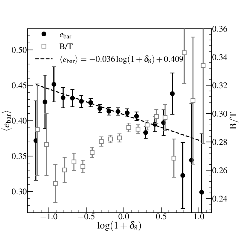
Figure 13: Dependence of mean bar strength $\langle e_{\mathrm{bar}}\rangle$ (black solid circles; left y-axis) and mean $\mathrm{B}/\mathrm{T}$ (gray open squares; right y-axis) on the spherical overdensity $\delta_{8}$. The black solid line is the best-fit linear relation between $\langle e_{\mathrm{bar}}\rangle$ and $\log(1+\delta_{8})$. All errorbars are $1{-}\sigma$ uncertainties estimated from Jackknife resampling.

In order to disentangle the effect of tidal anisotropy on bar strength from that of spherical overdensity, we remove the $\delta_{8}$-dependence of $\langle e_{\mathrm{bar}}\rangle$ by defining the average excess bar strength $\varepsilon$ at fixed $\alpha_{5}$ and $\delta_{8}$ as

$$\varepsilon(\alpha_{5},\delta_{8})\equiv\langle e_{\mathrm{bar}}\mid\alpha_{5},\,\delta_{8}\rangle-\langle e_{\mathrm{bar}}|\delta_{8}\rangle,$$ (8)

where $\langle e_{\mathrm{bar}}|\alpha_{5},\delta_{8}\rangle$ is shown in Figure 12 and $\langle e_{\mathrm{bar}}|\delta_{8}\rangle$ is calculated from the linear relation of Equation 7. Figure 14 shows the average excess bar strength in the low- and high-$\delta_{8}$ environments, $\varepsilon(\alpha_{5},\delta_{8}<0)$ (blue circles) and $\varepsilon(\alpha_{5},\delta_{8}\geq 0)$ (red squares), respectively, each as a function of $\log\alpha_{5}$. The errorbars are errors on the mean estimated from Jackknife resampling. For the majority ($98\%$) of galaxies that live in tidal environments with $\log\alpha_{5}<1$, their excess bar strength is consistent with zero, indicating that the anisotropy of their underlying tidal field does not play a role in the formation of bars. Interestingly, in the extreme tidal environments with $\log\alpha_{5}\geq 1$, the tidal dependence of bars in the underdense ($\delta_{8}<0$) vs. overdense ($\delta_{8}\geq 0$) environments deviate from zero and diverge in opposite directions — the bar strength of galaxies in the highly anisotropic, low-density regions is slightly boosted, while the bar strength in the equally high-$\alpha_{5}$ but high-density regions is somewhat hindered.

The straightforward interpretation is that the large-scale tidal anisotropy has no impact on the formation and evolution of bars, except for the two per cent of galaxies in the extreme tidal environments of $\log\alpha_{5}\geq 1$. In particular, fast-spinning haloes in those extreme tidal environments promote bar formation in the underdense regions, consistent with the predictions from simulations of galaxies in isolated haloes (Saha & Naab, 2013); Meanwhile in the overdense regions, fast-spinning haloes may suppress the growth of bars, as predicted by the cosmological simulations (Rosas-Guevara et al., 2022; Izquierdo-Villalba et al., 2022) where the galaxies are embedded in the dense cosmic web.

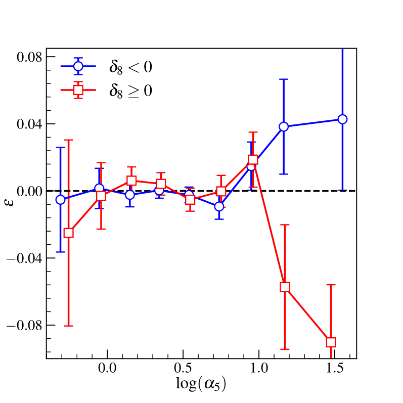
Figure 14: Dependence of the average excess bar strength $\varepsilon$ (defined in Equation 8) on $\alpha_{5}$ for galaxies in underdense ($\delta_{8}{<}0$; blue circles) and overdense ($\delta_{8}{\geq}0$; red squares) regions. All errorbars are $1-\sigma$ uncertainties estimated from Jackknife resampling.

However, although the non-zero signals at $\alpha_{5}{>}10$ is statistically significant (${>}1\sigma$), we caution that the Jackknife errorbars do not include any potential systematic errors from cosmic variance or the tidal anisotropy measurements. In particular, we use the same smoothing scale for computing $\alpha_{5}$ in both the low- and high-density regions, which could produce a differential aliasing effect that leads to some weak but $\delta_{8}$-dependent correlation between $\alpha_{5}$ and $\delta_{8}$. Since such a residual correlation cannot be removed by the estimator defined by Equation 8, it could potentially mimic the signal observed in Figure 14. Unfortunately, it is difficult to assess the impact of such a potential systematic error with a relatively sparse survey like the SDSS. Therefore, although the large-scale tidal dependence of bars is statistically detected above $1\sigma$ using the SDSS data, a denser galaxy sample within a larger volume is required for a smoking-gun detection of such an effect.

6 Conclusions

In this paper, we develop an automated bar detection method to measure the bar strength $e_{\mathrm{bar}}$ of galaxies by applying the ellipse fitting over galaxy images after subtracting the best-fitting 2D disc models. Compared with the conventional ellipse fitting scheme, our method is able to better reveal the strength of the underlying bars that are otherwise embedded in some of the bright discs. After performing an extensive suite of comparisons with the visual identifications using either SDSS or DESI imaging data, we find that our measurements of $e_{\mathrm{bar}}$ using disc-subtracted images are robust against the decrease in image quality and spatial resolution, and can thus be applied to SDSS images of galaxies up to $z{=}0.11$, the maximum redshift of our analysis.

To investigate the dependence of $e_{\mathrm{bar}}$ on the small-scale tidal environment, we make use of the cluster sample derived by the Y07 group catalogue from SDSS. Following the recent study of Y19, we divide the Y07 clusters into interacting vs. non-interacting systems, and measure the difference between the average bar strength $\langle e_{\mathrm{bar}}\rangle$ of galaxies surrounding interacting clusters and that around isolated ones. Within the same redshift range ($0.01{<}z{<}0.06$) probed by Y19, we confirm their results that the $\langle e_{\mathrm{bar}}\rangle$ in interacting clusters is higher than that in isolated systems. By examining the dependence of such enhancement on cluster mass and projected distance to the cluster centre, we find that the signal within $0.01{<}z{<}0.06$ is primarily contributed by galaxies in the central regions ($R{<}0.5R_{200c}$) of the few very massive cluster-cluster pairs ($\log M_{200c}{>}14.55$). However, after we increase the cluster sample by a factor of five by extending the analysis up to $z{=}0.11$, the tidal enhancement of bars in the interacting clusters goes away, indicating little correlation between the bar strength and cluster-scale tidal strength. This small-scale tidal analysis can be presumably extended to higher redshifts using photometric cluster catalogues (Golden-Marx et al., 2022), but the identification of cluster member galaxies will be subjected to strong projection effects (Zu et al., 2017).

For characterising the large-scale tidal environments, we adopt the tidal anisotropy parameter $\alpha_{5}$ calculated from the overdensity field smoothed over a scale of $5\,h^{-1}\mathrm{Mpc}$ (Paranjape et al., 2018). Assuming a large-scale tidal origin (at least partially) of the angular momentum of the haloes, we use $\alpha_{5}$ as a proxy for the spin of haloes in different anisotropic environments (Ramakrishnan et al., 2019). Following Alam et al. (2019), we compute $\alpha_{5}$ from a stellar mass-limited ($\log M_{*}{>}10$) galaxy sample between $0.01{<}z{<}0.074$, and measure the dependence of average bar strength $\langle e_{\mathrm{bar}}\rangle$ on $\alpha_{5}$ at fixed spherical (isotropic) overdensities. We do not detect any such dependence for $98\%$ of the galaxies residing in the environments with $\alpha_{5}{<}10$. Intriguingly, among the $2\%$ with $\alpha_{5}{\geq}10$, there is a hint of bar enhancement in the underdense regions, where the disc-halo systems are more likely to evolve in isolation. Since halo spin is correlated with the tidal anisotropy, this bar enhancement is consistent with the prediction by Saha & Naab (2013) that halo spin promotes bar formation/growth. In contrast, galaxies in the overdense regions exhibit suppressed bar strengths in the extremely anisotropic environments with $\alpha_{5}{\geq}10$, consistent with the prediction of some of the cosmological hydrodynamic simulations (Rosas-Guevara et al., 2022; Izquierdo-Villalba et al., 2022).

However, the non-zero signal at $\alpha_{5}{\geq}10$ is subjected to cosmic variance and systematic uncertainties associated with the tidal anisotropy measurements. For the cosmic variance, it could potentially be mitigated by using a constrained simulation (e.g., ELUCID; Wang et al., 2014) that accurately reproduces the underlying density field within the SDSS volume (see Salcedo et al., 2022, for a similar application). Looking to the future, both types of systematic errors can be better mitigated with the Bright Galaxy Survey (Hahn et al., 2022) within the Dark Energy Spectroscopic Instrument Survey (DESI; DESI Collaboration et al., 2022). Meanwhile, our automated bar detection method can be easily applied to upcoming space-based imaging surveys like the Chinese Survey Space Telescope (CSST; Gong et al., 2019) and the Roman Space Telescope (Roman; Spergel et al., 2015), both of which will provide sharp images of galactic bars within a cosmological volume up to much higher redshifts.

Combining our results on both small and large scales, we do not detect any strong evidence for the dependence of bar strength on the tidal field. Therefore, any tidal impact of bar formation, if exists, should be very weak in the local Universe. Together with the general lack of bar dependence on the overdensity environment Aguerri et al. (2009); Lee et al. (2012); Li et al. (2009); Skibba et al. (2012); Fraser-McKelvie et al. (2020), our conclusion has important implications for the theoretical understanding of bar formation — the primary driver of bar strength is most likely intrinsic to the disc galaxy itself, rather than the tidal environment, whether it be interacting clusters or tidal anisotropy.

Data Availability

The data underlying this article will be shared on reasonable request to the corresponding author.

References

- Abazajian et al. (2009) Abazajian K. N., et al., 2009, ApJS, 182, 543
- Aguerri et al. (2005) Aguerri J. A. L., Elias-Rosa N., Corsini E. M., Muñoz-Tuñón C., 2005, A&A, 434, 109
- Aguerri et al. (2009) Aguerri J. A. L., Méndez-Abreu J., Corsini E. M., 2009, A&A, 495, 491
- Alam et al. (2019) Alam S., Zu Y., Peacock J. A., Mandelbaum R., 2019, MNRAS, 483, 4501
- Athanassoula (1992) Athanassoula E., 1992, MNRAS, 259, 328
- Athanassoula (2002) Athanassoula E., 2002, ApJ, 569, L83
- Athanassoula (2003) Athanassoula E., 2003, MNRAS, 341, 1179
- Barazza et al. (2008) Barazza F. D., Jogee S., Marinova I., 2008, ApJ, 675, 1194
- Baxter et al. (2019) Baxter E. J., Sherwin B. D., Raghunathan S., 2019, J. Cosmology Astropart. Phys., 2019, 001
- Berentzen et al. (2004) Berentzen I., Athanassoula E., Heller C. H., Fricke K. J., 2004, MNRAS, 347, 220
- Binney & Tremaine (2008) Binney J., Tremaine S., 2008, Galactic Dynamics: Second Edition
- Bland-Hawthorn et al. (2023) Bland-Hawthorn J., Tepper-Garcia T., Agertz O., Freeman K., 2023, ApJ, 947, 80
- Blanton & Roweis (2007) Blanton M. R., Roweis S., 2007, AJ, 133, 734
- Blanton et al. (2005) Blanton M. R., et al., 2005, AJ, 129, 2562
- Bournaud & Combes (2002) Bournaud F., Combes F., 2002, A&A, 392, 83
- Brinchmann et al. (2004) Brinchmann J., Charlot S., White S. D. M., Tremonti C., Kauffmann G., Heckman T., Brinkmann J., 2004, MNRAS, 351, 1151
- Bruzual & Charlot (2003) Bruzual G., Charlot S., 2003, MNRAS, 344, 1000
- Byrd et al. (1986) Byrd G. G., Valtonen M. J., Sundelius B., Valtaoja L., 1986, A&A, 166, 75
- Catelan & Theuns (1996) Catelan P., Theuns T., 1996, MNRAS, 282, 436
- Cavanagh et al. (2022) Cavanagh M. K., Bekki K., Groves B. A., Pfeffer J., 2022, MNRAS, 510, 5164
- Chabrier (2003) Chabrier G., 2003, PASP, 115, 763
- Collier et al. (2018) Collier A., Shlosman I., Heller C., 2018, MNRAS, 476, 1331
- Cooray & Chen (2002) Cooray A., Chen X., 2002, ApJ, 573, 43
- DESI Collaboration et al. (2022) DESI Collaboration et al., 2022, AJ, 164, 207
- Debattista & Sellwood (2000) Debattista V. P., Sellwood J. A., 2000, ApJ, 543, 704
- Dey et al. (2019) Dey A., et al., 2019, AJ, 157, 168
- Doroshkevich (1970) Doroshkevich A. G., 1970, Astrophysics, 6, 320
- Earn & Lynden-Bell (1996) Earn D. J. D., Lynden-Bell D., 1996, MNRAS, 278, 395
- Efstathiou et al. (1982) Efstathiou G., Lake G., Negroponte J., 1982, MNRAS, 199, 1069
- Elmegreen & Elmegreen (1985) Elmegreen B. G., Elmegreen D. M., 1985, ApJ, 288, 438
- Erwin (2019) Erwin P., 2019, MNRAS, 489, 3553
- Fraser-McKelvie et al. (2020) Fraser-McKelvie A., et al., 2020, MNRAS, 499, 1116
- Fujii et al. (2018) Fujii M. S., Bédorf J., Baba J., Portegies Zwart S., 2018, MNRAS, 477, 1451
- Gadotti (2008) Gadotti D. A., 2008, MNRAS, 384, 420
- Gardner (2001) Gardner J. P., 2001, ApJ, 557, 616
- Gerin et al. (1990) Gerin M., Combes F., Athanassoula E., 1990, A&A, 230, 37
- Golden-Marx et al. (2022) Golden-Marx J. B., Zu Y., Wang J., Li H., Zhang J., Yang X., 2022, arXiv e-prints, p. arXiv:2212.13270
- Gong et al. (2019) Gong Y., et al., 2019, ApJ, 883, 203
- Hahn et al. (2022) Hahn C., et al., 2022, arXiv e-prints, p. arXiv:2208.08512
- Heavens & Peacock (1988) Heavens A., Peacock J., 1988, MNRAS, 232, 339
- Hernquist & Weinberg (1992) Hernquist L., Weinberg M. D., 1992, ApJ, 400, 80
- Hetznecker & Burkert (2006) Hetznecker H., Burkert A., 2006, MNRAS, 370, 1905
- Hohl (1971) Hohl F., 1971, ApJ, 168, 343
- Hu & Kravtsov (2003) Hu W., Kravtsov A. V., 2003, ApJ, 584, 702
- Izquierdo-Villalba et al. (2022) Izquierdo-Villalba D., et al., 2022, MNRAS, 514, 1006
- Jang & Kim (2023) Jang D., Kim W.-T., 2023, ApJ, 942, 106
- Jedrzejewski (1987) Jedrzejewski R. I., 1987, MNRAS, 226, 747
- Jing et al. (2007) Jing Y. P., Suto Y., Mo H. J., 2007, ApJ, 657, 664
- Jogee et al. (2004) Jogee S., et al., 2004, ApJ, 615, L105
- Kalnajs (1972) Kalnajs A. J., 1972, ApJ, 175, 63
- Kataria & Das (2018) Kataria S. K., Das M., 2018, MNRAS, 475, 1653
- Kataria & Shen (2022) Kataria S. K., Shen J., 2022, ApJ, 940, 175
- Kataria et al. (2020) Kataria S. K., Das M., Barway S., 2020, A&A, 640, A14
- Kauffmann et al. (2003) Kauffmann G., et al., 2003, MNRAS, 341, 33
- Kormendy & Kennicutt (2004) Kormendy J., Kennicutt Robert C. J., 2004, ARA&A, 42, 603
- Laine et al. (2002) Laine S., Shlosman I., Knapen J. H., Peletier R. F., 2002, ApJ, 567, 97
- Laurikainen et al. (2005) Laurikainen E., Salo H., Buta R., 2005, MNRAS, 362, 1319
- Lee et al. (2012) Lee G.-H., Park C., Lee M. G., Choi Y.-Y., 2012, ApJ, 745, 125
- Li et al. (2009) Li C., Gadotti D. A., Mao S., Kauffmann G., 2009, MNRAS, 397, 726
- Li et al. (2011) Li Z.-Y., Ho L. C., Barth A. J., Peng C. Y., 2011, ApJS, 197, 22
- Long et al. (2014) Long S., Shlosman I., Heller C., 2014, ApJ, 783, L18
- Lupton et al. (2004) Lupton R., Blanton M. R., Fekete G., Hogg D. W., O’Mullane W., Szalay A., Wherry N., 2004, PASP, 116, 133
- Lynden-Bell (1979) Lynden-Bell D., 1979, MNRAS, 187, 101
- Maller et al. (2002) Maller A. H., Dekel A., Somerville R., 2002, MNRAS, 329, 423
- Marinova & Jogee (2007) Marinova I., Jogee S., 2007, ApJ, 659, 1176
- Martin (1995) Martin P., 1995, AJ, 109, 2428
- Martinez-Valpuesta et al. (2017) Martinez-Valpuesta I., Aguerri J. A. L., González-García A. C., Dalla Vecchia C., Stringer M., 2017, MNRAS, 464, 1502
- Masters et al. (2011) Masters K. L., et al., 2011, MNRAS, 411, 2026
- Menéndez-Delmestre et al. (2007) Menéndez-Delmestre K., Sheth K., Schinnerer E., Jarrett T. H., Scoville N. Z., 2007, ApJ, 657, 790
- Miwa & Noguchi (1998) Miwa T., Noguchi M., 1998, ApJ, 499, 149
- Nair & Abraham (2010) Nair P. B., Abraham R. G., 2010, ApJS, 186, 427
- Noguchi (1987) Noguchi M., 1987, MNRAS, 228, 635
- Noguchi (1988) Noguchi M., 1988, A&A, 203, 259
- Ostriker & Peebles (1973) Ostriker J. P., Peebles P. J. E., 1973, ApJ, 186, 467
- Paranjape et al. (2018) Paranjape A., Hahn O., Sheth R. K., 2018, MNRAS, 476, 3631
- Peebles (1969) Peebles P. J. E., 1969, ApJ, 155, 393
- Peschken & Łokas (2019) Peschken N., Łokas E. L., 2019, MNRAS, 483, 2721
- Porciani et al. (2002) Porciani C., Dekel A., Hoffman Y., 2002, MNRAS, 332, 325
- Prieto et al. (2001) Prieto M., Aguerri J. A. L., Varela A. M., Muñoz-Tuñón C., 2001, A&A, 367, 405
- Ramakrishnan et al. (2019) Ramakrishnan S., Paranjape A., Hahn O., Sheth R. K., 2019, MNRAS, 489, 2977
- Rosas-Guevara et al. (2022) Rosas-Guevara Y., et al., 2022, MNRAS, 512, 5339
- Saha & Naab (2013) Saha K., Naab T., 2013, MNRAS, 434, 1287
- Salcedo et al. (2022) Salcedo A. N., et al., 2022, Science China Physics, Mechanics, and Astronomy, 65, 109811
- Savitzky & Golay (1964) Savitzky A., Golay M. J. E., 1964, Analytical Chemistry, 36, 1627
- Sellwood (1981) Sellwood J. A., 1981, A&A, 99, 362
- Sellwood (2014) Sellwood J. A., 2014, Reviews of Modern Physics, 86, 1
- Simard et al. (2011) Simard L., Mendel J. T., Patton D. R., Ellison S. L., McConnachie A. W., 2011, ApJS, 196, 11
- Skibba et al. (2012) Skibba R. A., et al., 2012, MNRAS, 423, 1485
- Spergel et al. (2015) Spergel D., et al., 2015, arXiv e-prints, p. arXiv:1503.03757
- Stoughton et al. (2002) Stoughton C., et al., 2002, AJ, 123, 485
- Strauss et al. (2002) Strauss M. A., et al., 2002, AJ, 124, 1810
- Toomre (1981) Toomre A., 1981, in Fall S. M., Lynden-Bell D., eds, Structure and Evolution of Normal Galaxies. pp 111–136
- Vitvitska et al. (2002) Vitvitska M., Klypin A. A., Kravtsov A. V., Wechsler R. H., Primack J. R., Bullock J. S., 2002, ApJ, 581, 799
- Walmsley et al. (2022) Walmsley M., et al., 2022, MNRAS, 509, 3966
- Wang et al. (2011) Wang H., Mo H. J., Jing Y. P., Yang X., Wang Y., 2011, MNRAS, 413, 1973
- Wang et al. (2014) Wang H., Mo H. J., Yang X., Jing Y. P., Lin W. P., 2014, ApJ, 794, 94
- Wang et al. (2022) Wang J., et al., 2022, ApJ, 936, 161
- Weinberg (1985) Weinberg M. D., 1985, MNRAS, 213, 451
- White (1984) White S. D. M., 1984, ApJ, 286, 38
- Willett et al. (2013) Willett K. W., et al., 2013, MNRAS, 435, 2835
- Wozniak et al. (1995) Wozniak H., Friedli D., Martinet L., Martin P., Bratschi P., 1995, A&AS, 111, 115
- Yang et al. (2005) Yang X., Mo H. J., van den Bosch F. C., Jing Y. P., 2005, MNRAS, 356, 1293
- Yang et al. (2007) Yang X., Mo H. J., van den Bosch F. C., Pasquali A., Li C., Barden M., 2007, ApJ, 671, 153
- Yoon et al. (2019) Yoon Y., Im M., Lee G.-H., Lee S.-K., Lim G., 2019, Nature Astronomy, 3, 844
- York et al. (2000) York D. G., et al., 2000, AJ, 120, 1579
- Zhao et al. (2020) Zhao D., Du M., Ho L. C., Debattista V. P., Shi J., 2020, ApJ, 904, 170
- Zu & Mandelbaum (2015) Zu Y., Mandelbaum R., 2015, MNRAS, 454, 1161
- Zu et al. (2017) Zu Y., Mandelbaum R., Simet M., Rozo E., Rykoff E. S., 2017, MNRAS, 470, 551
- de Vaucouleurs (1963) de Vaucouleurs G., 1963, ApJS, 8, 31
- van der Kruit & Freeman (2011) van der Kruit P. C., Freeman K. C., 2011, ARA&A, 49, 301