A gravitational constant transition within cepheids as supernovae calibrators can solve the Hubble tension

Abstract

Local universe measurements of the Hubble constant $H_{0}$ using SNe Ia with Cepheids as calibrators yield a value of $H_{0}$ = 73.04 $\pm$ 1.04 km s^-1 Mpc^-1, which is in tension with the value of $H_{0}$ inferred from the Cosmic Microwave Background and other higher redshift probes. In ref. [1], the authors proposed a rapid transition in the value of the effective Newtonian gravitational constant $G$ in order to alleviate the Hubble tension. The transition point was chosen so as to only affect distance estimates to Hubble flow SNe. However, in this study, the authors made the assumption that SNe Ia peak luminosity $L$ increases with Chandrasekhar mass $M_{c}$. This hypothesis contradicts a previous semi-analytic study of SN light curves in the presence of a $G$-transition [2] which concluded that there is an inverse relationship between $L$ and $M_{c}$. Motivated by the results of ref. [1] and [2], we propose a hypothesis of a sudden recent change in the effective Newtonian gravitational constant $G$ at an epoch which corresponds to a smaller look-back distance between $\sim$ 7 - 80 Mpc. A transition in $G$ at these distances would affect both our estimates of the distances to Cepheids in calibrator galaxies, as well as to the Hubble flow supernovae. Upon fitting the observational data to this hypothesis, we find three interesting results: (i) we find mild evidence for a $G$-transition at 22.4 Mpc (73 million years ago) which is preferred (using certain estimators) by the calibrator type Ia SNe data over no $G$-transition, (ii) the $H_{0}$ parameter inferred under this hypothesis is in good agreement with the value obtained from the CMB for a 4% larger value of $G$ at earlier times, thus potentially resolving the Hubble tension, (iii) we obtain a fit to the scaling relationship between SN peak luminosity $L$ and Chandrasekhar mass $M_{c}$, as $L\propto M_{c}^{-1.68\pm 0.68}$, which is in good agreement with the prediction of the theoretical study of ref. [2]. We also discuss how other probes could be used to verify this transition in the value of $G$.

1 Introduction

The measurement of the Hubble constant $H_{0}$ is of fundamental importance to calibrate our cosmological models. $H_{0}$ can be inferred either directly from low-redshift probes of the expansion rate of the local universe, or it can be inferred indirectly through measurements of high redshift observables such as the Cosmic Microwave Background (CMB) and Baryon Acoustic Oscillations (BAO). The local measurement of $H_{0}$ from the Cepheid-calibrated type Ia Supernovae (SNe Ia), as performed by the SH0ES’22 collaboration [3] yields a value of $H_{0}=73.04\,\pm\,1.04$ km s^-1 Mpc^-1(68% C.L.). In contrast, the high redshift measurements from CMB and BAO yield a lower value of $H_{0}=67.66\,\pm\,0.42$ km s^-1 Mpc^-1(68% C.L.) [4]. These two values are discrepant at the 5-$\sigma$ level. This discrepancy between these estimated values of the Hubble constant $H_{0}$ from the local universe and CMB measurements is called the “Hubble tension”. Resolving this discrepancy is one of the major open problems in cosmology.

The low-redshift probes rely on the assumption of a “standard candle” which are type Ia supernovae. The distances to these objects can not be calibrated by a direct method such as parallax measurements, and therefore another intermediate calibrator is needed. Cepheid variables, which have been shown to have a robust period-luminosity relationship (PLR) and can be seen out to large distances, have been used as calibrators in the SH0ES analysis [3].

It is possible that unknown systematics in the physics of Cepheid calibrators could perhaps be responsible for the discrepancy in the inferred value of $H_{0}$. The Carnegie-Chicago Hubble Project (CCHP) collaboration has attempted to measure the $H_{0}$ parameter using SNe Ia calibrated to stars at the tip of the red-giant branch (TRGB), and they obtained a value of $H_{0}=69.8\pm 0.8\leavevmode\nobreak\ (\textrm{stat})\pm 1.7\leavevmode\nobreak\ (\textrm{sys})$ km s^-1 Mpc^-1(68% C.L.) [5, 6], which lies between the values reported by SH0ES [7, 8, 3, 9] and the Planck 2018 results [4] and can be taken to agree with either within 2$\sigma$. However, a revised calibration of TRGBs using the parallax measurement of $\omega-$Centauri from GAIA EDR3 yields a value of $H_{0}=72.1\pm 2.0$ km s^-1 Mpc^-1(68% C.L.) [10, 11], which makes both the local CCHP measurement and SH0ES measurement consistent with each other, while still indicating a tension between the low-redshift and high-redshift measurements.

Other local measurements from quasar strong lensing, dispersion of fast radio burst signals, and gravitational wave observations have not yet achieved the precision needed to weigh in on the discrepancy. A joint analysis of $6$ strongly lensed quasars with measured time delays yielded $H_{0}=73.3^{+1.7}_{-1.8}$ km s^-1 Mpc^-1[12]. An analysis of a set of $9$ currently available Fast Radio Burst (FRB) [13] samples yielded $H_{0}=62.3\pm 9.1$ km s^-1 Mpc^-1. Recent gravitational wave events with the first and second observing runs at the advanced LIGO/Virgo along with binary black hole detections in conjunction with galaxy catalogs have found $H_{0}=68.7^{+17.0}_{-7.8}$ km s^-1 Mpc^-1[14].

A number of studies have been conducted to understand if as yet unknown systematic effects in the measurements of the local universe are the cause of the Hubble tension [15, 16, 17, 18, 19, 20, 21, 22, 23]. However, accounting for these systematic effects does not seem to resolve the tension.

Given that the Hubble tension is unlikely to be resolved with standard physics alone, a variety of new physics solutions have been proposed that attempt to resolve this tension (see [24] and the references therein). These solutions can, broadly, be classified into two types, depending on where the new physics has its strongest effect, as pre-recombination and post-recombination solutions [25]. While some of the proposed solutions ameliorate the Hubble tension, there are no known solutions that can fully resolve it (i.e. reduce the discrepancy to less than 1$\sigma$ without creating other discrepancies) [26].

In this work, we focus on a sharp transition in the gravitational constant ($G$) in the very late universe, as a potential solution to the $H_{0}$ tension. Such a late transition in the gravitational constant would, among other things, change the physics of Cepheids and SNe Ia, thus modifying our inferred distance measurements, and hence the value of the inferred Hubble constant.

Our motivation to study the effects of such a transition stems from a series of other works which have discussed the possibility of a $G$-transition in the late universe.

• In [27] and [28], the authors discussed how changes in the effective gravitational constant due to screened fifth forces can cause changes in the dynamics of Cepheids and TRGB stars respectively, which can potentially solve the Hubble tension. However, in this work, the authors did not assume a sharp transition in $G$, but rather a local environmental dependence on $G$ using the fifth force mechanism. They could alleviate the Hubble Tension to below $3\sigma$ but not less than 2$\sigma$ while maintaining self-consistency of the distance ladder.

• In [1], the authors argued how the Hubble tension can be interpreted as a tension in the inferred absolute magnitude ($M_{B}$) of distant SNe Ia which lie in the Hubble flow. Such an effect could arise due to a rapid transition in the gravitational constant at a certain transition redshift.

• From a theoretical perspective, a sharp transition in the gravitational constant $G$ can arise from scalar-tensor theories with a step-like potential with an abrupt feature in the functional form of the non-minimal coupling function [29].

In the present work, we study the possibility of a late-time $G$-transition at look-back times corresponding to a distance between $\sim$ 7 - 80 Mpc (23 million to 260 million years ago). Such a late transition would not only affect the physics of SNe Ia, but it would also affect the distances to standard calibrators such as Cepheids and TRGB stars. Thus, our hypothesis of new physics is distinct from the work of [1] which considered a change which can only affect type Ia SNe. Our hypothesis is also distinct from that of [27] and [28] which only considered a change in the physics of Cepheids and TRGBs due to an environmental $G$ dependence.

While the effect of a $G$-transition on the Cepheid PLR can be easily modelled and used to recalibrate the distance ladder to Cepheids, the effect of a $G$-transition on the luminosity of type Ia supernovae is more uncertain. The key effect of a $G$-transition is that it would change the Chandrashekhar mass $M_{c}$, and type Ia SNe luminosities are assumed to grow with $M_{c}$. However, the precise form of the scaling relation is unknown. Wright and Li [2] in a theoretical study with non-standard gravity argued that the standardized SN peak luminosity decreases with an increase in the Chandrasekhar Mass $M_{c}$ rather than increasing. They found that the scaling relation of the standardized SN luminosity with $M_{c}$ is $L\sim M_{c}^{-0.97}$ [30].

We perform a fit similar in spirit to that of the SH0ES collaboration [8] to Cepheids and SNe Ia observational data, but under the modified hypothesis of a late-time $G$-transition. Rather than assuming a specific scaling relation of $L$ with $M_{c}$, we parameterize the scaling relation of type Ia SNe as $L\sim M_{c}^{n}$, and we leave $n$ as a fit parameter. Upon fitting the low redshift data to this hypothesis, we find three interesting results – (i) we find mild evidence that the $G$-transition that we propose is preferred by the type Ia SNe data over no $G$-transition, (ii) the $H_{0}$ parameter inferred under this hypothesis is in good agreement with the value obtained from the CMB for a 4% larger value of $G$ at earlier times, thus potentially resolving the Hubble tension, (iii) we obtain a fit to the scaling relationship between SN peak luminosity $L$ and Chandrasekhar mass $M_{c}$, as $L\propto M_{c}^{-1.68\pm 0.68}$, which is in agreement with the prediction of the theoretical study of ref. [2].

Our results suggest circumstantial evidence for a late time $G$-transition as a solution to the Hubble tension. We also discuss further tests that could be performed to confirm, or rule out the $G$-transition hypothesis.

This paper is structured as follows. In section 2, we give analytic arguments for the effect of a $G$-transition on the inference of the Hubble constant, through the effects on the Cepheid period-luminosity relation (PLR), the SNe Ia luminosity, and the consequent effect on distance ladder inferences. In section 3, we outline the methodology that we will use in performing our fit to the distance ladder in the presence of a $G$-transition. Then in section 4, we discuss the observational data sets of Cepheids and supernovae used for fitting the distance ladder. In section 5, we first reproduce the results of our distance ladder fit assuming the standard cosmology without a $G$-transition. Our analysis procedure is a simplified version of that of SH0ES’22  [3]. After validating our analysis strategy we then proceed in section 6 to discuss the change to our analysis method that is needed when taking into account the possibility of a $G$-transition. In the same section, we also show the results of our analysis when including a $G$-transition. We demonstrate two of our main claims that we have stated above, about resolving the Hubble tension and our inference of the $L$-$M_{c}$ relation in this section. In section 7, we use different fit comparison techniques like $\chi^{2}_{\textrm{dof}}$, AIC, and BIC to understand the preference in the data for a $G$-transition hypothesis over the null hypothesis of the no $G$-transition scenario. We finally conclude with some discussion on implications of our results and further tests in section 8.

2 The distance ladder and the effect of a $G$- transition

In the local universe, the expansion rate can be approximately described by a linear relation $v=H_{0}\,r$. Here, $v$ is the recession velocity of a galaxy located at a distance $r$. This is commonly known as the Hubble - Lemaître law [31, 32] or Hubble law in short. The value of $H_{0}$ can be determined by finding the recession velocities and distances to distant objects and fitting to the linear relationship expected from the Hubble law. Velocities can be measured by redshifts of characteristic spectral lines and distances can be measured by constructing a distance ladder through some standardized astrophysical objects. In order for the Hubble law to hold, distances (or redshifts) need to be large enough so that the recession velocity is larger than the peculiar motions due to local gravitational flows. Typically this condition is satisfied for galaxies at redshifts $z\gtrsim 0.01$, for which the recession velocity is primarily due to cosmic expansion. Such galaxies are said to belong to the “Hubble flow”. Thus, $H_{0}$ can be determined by fitting a distance-redshift relation to galaxies in the Hubble flow.

A transition in the gravitational coupling constant will affect the astrophysics of standard objects used in constructing the distance ladder. Note that since spectral emission/absorption lines depend only on atomic physics, redshift values of galaxies are insensitive to a change in $G$. Thus, the primary effect of a $G$-transition, as far as the inference of the Hubble constant is concerned, is that it modifies the inferred distances that we extract from the distance ladder.

In the rest of this section, we will describe how the standard cosmic distance ladder is constructed using observations of Cepheid variables and SNe Ia explosions. We will then discuss how distance measurements, and consequently the inferred value of $H_{0}$, would be affected by a sudden $G$-transition. Our treatment in this section is purely analytic so as to clearly delineate the effect of a $G$-transition on the inference of the Hubble constant.

2.1 The standard distance ladder

The Supernovae and $H_{0}$ for dark energy Equation of State (SH0ES) collaboration has claimed the most precise local measured value of $H_{0}$ [9, 7, 8]. The SH0ES team primarily studied luminous type Ia SNe in the Hubble flow which are well known to be “standardizable candles” [33, 34] . The following discussion will describe the strategy for the SH0ES analysis and how they establish a distance ladder to calibrate type Ia SNe.

The progenitor for an SN Ia explosion is believed to be accretion or merger of a white dwarf in a binary system [35]. When the white dwarf nears the Chandrashekhar mass, it undergoes runaway nuclear fusion that unbinds the star in a catastrophic explosion. Because of the fixed critical mass of the progenitor, type Ia SNe are expected to have a standard luminosity, i.e. they are expected to be standard candles [36]. If we know this standard expected luminosity, then we can combine this with the flux measurement from observed type Ia SNe to measure distances to galaxies in the Hubble flow which host such SNe.

Observed type Ia SNe explosions have variable peak luminosities and therefore are not truly standard candles [33, 34]. However, the peak luminosities are tightly (positively) correlated with the decay time of the light curve for such SNe [33, 34]. Observations of Hubble flow SNe at a given redshift indicate that “stretching” the light curves to agree with the shape of a template light curve yields nearly identical light curves [37, 38]. This allows us to standardize the light curves to a template at a given redshift. Moreover this standardization of the light curves to a given template (with a suitable redshift correction to the apparent magnitude) works at all redshifts in the Hubble flow, indicating very little evolution [39] with redshift of the intrinsic standardized type Ia SNe light curve (after taking into account various other corrections like dust extinction, coherent flows in the local universe etc.).

If we knew the intrinsic peak luminosity of the standardized template, we could use this to infer the distance to type Ia SNe. Thus, type Ia SNe are referred to as “standardizable candles”. In order to use type Ia SNe to measure the Hubble constant, one needs to first calibrate the standardized peak luminosity of nearby SNe Ia. The peak luminosity can then be inferred from a combination of knowledge of the flux and distance to a type Ia SN in a nearby galaxy. Distances within our galaxy and nearby galaxies can be directly determined with high precision through either trigonometric parallaxes [40, 8], Detached Eclipsing Binaries (DEBs) [41], or water MASERs [42]. However, no SN Ia explosion has been observed to which such a direct distance measurement is available.

Thus, the standard Type Ia SNe luminosity needs to be calibrated with an intermediary. The SH0ES collaboration uses classical Cepheid variables as the intermediary. Cepheids are pulsating stars, where the pulsations are driven by the Eddington valve or $\kappa$-mechanism [43, 44]. Cepheid variables as discovered by Henrietta Leavitt have a well defined Period - Luminosity Relation (PLR) which allows them to be used as standard candles [45, 46]. Moreover, Cepheids are bright enough to be observable out to large extra-galactic distance scales with the Hubble Space Telescope [47, 9]. This makes it possible to find a sample of galaxies which a) host a SN Ia explosion, and b) contain a large number of Cepheid variables. The distances to these “calibrator” galaxies can be determined using the Cepheid PLR and then the SNe Ia luminosity can be derived. In order to use Cepheids to calibrate type Ia SNe, the standard Cepheid PLR needs to be first determined using observations of Cepheids in nearby “anchor” galaxies to which direct distance measurements are available.

Thus, the SH0ES analysis of type Ia SNe in the Hubble flow to measure the Hubble constant uses a distance ladder which involves the following three steps:

• Anchor step: This step involves calibrating the standard Cepheid PLR with the help of geometric distances. Cepheids in the MilkyWay (MW) and nearby galaxies like the Large Magellanic Cloud (LMC) and NGC4258 are used for this purpose. For Cepheids in the MW, LMC, and NGC4258, SH0ES uses trigonometric parallax based distances [40, 8], DEB based distances [48, 7], and water MASER based distances [49, 9], respectively. Knowledge of these distances along with the measured fluxes and periods of the Cepheids yields the PLR. The anchor objects have distances up to approximately 7 Mpc.

• Calibrator step: This involves calibrating the SNe Ia luminosity with the Cepheid PLR. A set of $37$ calibrator galaxies which have had SNe Ia explosions and also contain Cepheid variables are used for this purpose [3]. The PLR derived from anchors, along with the measured Cepheid periodicity is used to infer distances to these calibrator galaxies. These distances combined with the corrected peak apparent magnitudes of type Ia SNe yield their intrinsic standardized peak-luminosity. The calibrator galaxies range in distances from approximately 7 Mpc to 80 Mpc.

• Hubble flow step: Finally, the standardized luminosity of SNe Ia are used to infer the distances to Hubble flow SNe. By measuring the redshift of the host galaxies, SH0ES finds a distance-redshift relation for several hundred SNe Ia in the Hubble flow and they use this to determine the value of $H_{0}$. It includes SNe Ia ranging from redshift $z=0.023$ to $z=0.15$ (corresponding to distances $>$ 80 Mpc).

In practice, the SH0ES team performs a simultaneous fit to data for the anchors, calibrators, and Hubble flow objects. In the next sub-section, we will explain how a $G$-transition will affect this distance ladder, and alter the inference of the Hubble constant.

2.2 Effect of a $G$-transition on the distance ladder

We define a gravitational constant ($G$) transition as a sudden change in the value of $G$ at some cosmic epoch. The value of $G$ at the present epoch is taken to be $G_{N}=6.67\times 10^{-11}$ N-m/kg² as measured in terrestrial experiments [50]. Our hypothesis is thus, that at a lookback time corresponding to some transition distance $d_{t}$, the effective universal gravitational constant was larger by an amount $\Delta G$. Here, $d_{t}$ and $\Delta G$ are parameters of our model. In the rest of this article whenever we refer to objects which lie to the left or to the right of the transition, this should be taken to mean objects at $d<d_{t}$ or $d>d_{t}$, respectively.

If the $G$-transition occurs sufficiently late in our cosmological history, i.e. for sufficiently low $d_{t}$, below a few 100 Mpc, it would directly affect the properties of the objects that constitute the distance ladder beyond $d_{t}$, and hence alter the inferred value of $H_{0}$. Depending on the precise value of $d_{t}$, it would modify the standardized SNe Ia peak-luminosity for some/all Hubble flow supernovae, or for sufficiently low $d_{t}$, it could possibly even alter the Cepheid PLRs.

A transition at $d_{t}>80$ Mpc would affect the standardization of type Ia SNe light curves in the Hubble flow and might be in conflict with observations which have indicated no evolution in SNe Ia light curve properties. A transition distance $d_{t}=80$ Mpc at the boundary between calibrators and the Hubble flow SNe was proposed in ref. [1] in an attempt to solve the Hubble tension. However, in order to alleviate the tension, this study assumed a peak-luminosity - Chandrashekhar mass relation $L\propto M_{c}$, an assumption which is in contradiction with the results of the semi-analytic model of ref. [2] which indicates an inverse relationship between $L$ and $M_{c}$.

In the present work, we focus on a transition that occurs within the set of calibrator galaxies which lie at distances between $\sim 7$ - $80$ Mpc (SH0ES refers to this as the calibrator rung of the distance ladder) in such a way that some calibrators lie beyond the distance $d_{t}$. This would lead to different properties of the nearby Cepheids and SNe, as compared to those beyond $d_{t}$. Cepheids and SNe Ia can still be used as standard candles, but their standard calibrations will be different before and after the epoch of $G$-transition. Thus, if the hypothesis of a $G$-transition is correct, not accounting for the change in properties of the distant Cepheids and SNe Ia would lead to an incorrect inference of their distances and hence an incorrect inference of the Hubble constant. This could potentially explain the discrepancy between the local and distant universe measurements of $H_{0}$.

In the next two sub-sections, we first explain how a $G$-transition would change the Cepheid PLR and SNe Ia standardized peak luminosity. We will then explain, for each of these objects, how not taking into account these changes would lead to an incorrect inference of the distances to their host galaxies. Then in the last sub-section, we explain how the incorrectly inferred distances would lead to an incorrectly inferred Hubble constant.

Next, we explain how the Cepheid PLR and SNe Ia peak luminosity depend on the value of $G$.

2.2.1 The Cepheid PLR and a $G$-transition

Cepheids are variable stars, which populate the upper region of the instability strip in the optical color-magnitude parameter space [51]. Cepheid variables act as standard candles for extra-galactic distance determination because of their tight period-luminosity relation [45, 46]. They are also luminous enough in order to be observable out to large extra-galactic distance scales up to $80$ Mpc with the Hubble Space Telescope (HST) [9, 3]. The Cepheid PLR more generally can be expressed as a period-luminosity-color relation (PLCR) as follows [44],

$$\log(L)=a\log\left(\frac{P\>\rm{(days)}}{10\>\rm{days}}\right)+b\log\left(T_{\textrm{eff}}\right)+c$$ (2.1)

here $L$ is the mean luminosity, $P$ is the pulsation period, and $T_{\textrm{eff}}$ is the effective surface temperature of the Cepheid which can be replaced by observable colour. Here, $a$, $b$, and $c$ are coefficients that determine the PLCR. When Cepheids are observed in a given wavelength band (colour or effective temperature is fixed), the $3$-dimensional PLCR gets projected on to the $2$-dimensional period-luminosity plane and this leads to the PLR [44],

$$\log(L)=\alpha\log\left(\frac{P\>\rm{(days)}}{10\>\rm{days}}\right)+\gamma.$$ (2.2)

The coefficient $\alpha$ (which is positive) determines the slope of the PLR and $\gamma$ is the intercept. The coefficient $\gamma$ can also be thought of as the logarithm of the luminosity of a classic Cepheid variable with a period $P=10$ days.

Effect of a $G$-transition on the Cepheid PLR

If the effective $G$ were different, this would change both the pulsation period, as well as the luminosity of a Cepheid. The resulting changes in the Cepheid period and luminosity would modify the Cepheid PLR.

The dynamics of Cepheid pulsations, and hence the pulsation period, are governed by the helium partial ionization zone which lies in the envelope of the star. On the other hand, the luminosity of the Cepheid is dictated by nuclear burning in the core [44]. Thus, the change in the period and the change in mean luminosity can be analyzed independently to a good approximation.

Ritter [52] for the first time demonstrated that the pulsating period of a homogeneous sphere undergoing adiabatic radial pulsation varies with the mean surface density of the sphere as $P\propto\sqrt{R/g}$ where $R$ is the radius of the gaseous sphere and $g$ is the surface gravity. Later, many studies [44, 53, 43, 54] showed that this relationship is also valid for real stars. Heuristically, the pulsation period can be set proportional to the free-fall time of the Cepheid envelope, which scales as $P\propto 1/\sqrt{G\overline{\rho}}$ [30], where $\overline{\rho}$ is the mean density. If we implicitly assume that the mean density is unchanged by a change in $G$, this would lead to a scaling relation $P\propto 1/\sqrt{G}$. This implies that if the change in effective $G$ is $\Delta G$, the change in Cepheid period would be,

$$\Delta\log(P)=-\frac{1}{2}\log\left(1+\frac{\Delta G}{G_{N}}\right),$$ (2.3)

where $G_{N}$ is the Newtonian gravitational constant. In particular for a positive change $\Delta G$, the Cepheid period would decrease.

Now let us discuss the change in luminosity of a Cepheid due to a change in $G$. Cepheid variables burn a H-shell surrounding an inert He core (although, some amount of He core burning can take place) [44]. For a fixed Cepheid mass, a slight increase in the effective gravitational constant would require more pressure support to maintain hydrostatic equilibrium. This pressure support can only be generated by increased nuclear burning in the core. The net result would therefore be an increase in luminosity.

Sakstein et al. [30] ran simulations with the MESA (Modules for Experiments in Stellar Astrophysics) [55] code, by modifying $G$ in the Cepheid cores. They obtained an expression for the change in luminosity at the blue edge of the instability strip which is of the form,

$$\Delta\log L=B\,\log(1+\Delta G/G_{N}),$$ (2.4)

where the value of the coefficient $B$ depends on the mass of the Cepheid as well as which crossing of the instability strip is being considered. In ref. [30] the authors tabulated values of $B$ as a function of the stellar mass and the instability strip crossing epoch. The typical values of $B$ that they obtained were between $3.46$ and $4.52$. Since $B$ is positive, this implies an increase in luminosity for an increase in the effective gravitational constant.

The change in Cepheid PLR due to a change in $G$ can now be understood through a combination of the changes in the period and luminosity of a given Cepheid. To illustrate this, we show a schematic diagram of the Cepheid PLR in fig. 1. The blue line in the figure represents the standard Cepheid PLR when the gravitational constant is $G_{N}$.

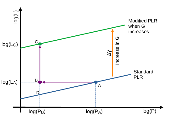
Figure 1: Illustration of how the Cepheid PLR would change if the effective $G$ were to increase. The original Cepheid PLR is shown in blue. Under an increase in $G$, a Cepheid at point A would have its period decrease and luminosity increase so that it would move to point $C$. By similar consideration for all other Cepheids, we would find that the effective PLR would be modified from the blue line to the green line, which has an identical slope to the original PLR but has an intercept difference $\Delta\gamma$. For Cepheids beyond the transition distance $d_{t}$, they would follow the green PLR. If we incorrectly used the low distance blue PLR to infer their luminosities from their periods, we would underestimate the true Log luminosity by an amount $\Delta\gamma$.

Now consider a specific Cepheid at point $A$ with luminosity $L_{A}$ and period $P_{A}$. What happens to the the period and luminosity for this Cepheid after a change in $G$? The period of the Cepheid would change to $P_{B}$, where $\log(P_{\textrm{B}})-\log(P_{\textrm{A}})=-\frac{1}{2}\log(1+\frac{\Delta G}{G_{N}})$ and its luminosity would increase from $L_{A}$ to $L_{C}$, where $\log(L_{\textrm{C}})-\log(L_{\textrm{A}})=B\,\log(1+\Delta G/G_{N})$. This change is shown in the figure as a two step change with first the change in period only (point $B$), followed by a change in luminosity (point $C$). Thus, the Cepheid’s position on the period-luminosity diagram would change to point $C$. Repeating this procedure for all Cepheids on the original PLR, we would obtain the modified PLR relation (shown as the green curve in the figure),

$$\log(L)=\alpha\log\left(\frac{P\>\rm{(days)}}{10\>\rm{days}}\right)+\gamma+\Delta\gamma,$$ (2.5)

where the change in the PLR intercept $\Delta\gamma$ is

$$\Delta\gamma=\left(\frac{\alpha}{2}+B\right)\log\left(1+\frac{\Delta G}{G_{N}}\right).$$ (2.6)

Thus, the net effect of a positive $(\Delta G>0)$ $G$-transition is a modified Cepehid PLR with exactly the same slope as the original PLR but an increased intercept.

Error in distance measurements due to assumption of a single PLR in the presence of a $G$-transition

Now under our hypothesis of $G=G_{N}$ at distances below $d_{t}$, and $G=G_{N}+\Delta G$ at distances larger than $d_{t}$, we can ask what incorrect inference would we make about the distances to Cepheids if we assumed a single PLR was valid at all distances?

Assuming that the calibration of Cepheids at lower distances yielded a PLR similar to the blue line in figure 1, Cepheids beyond the transition distance $d_{t}$ would actually obey the modified (green) PLR. If we incorrectly used the blue PLR to infer the luminosity for a given observed pulsation period, we would underestimate $\log L$ by the PLR intercept offset $\Delta\gamma$.

Thus, for $\Delta G$ positive we would underestimate the intrinsic luminosity of Cepheids beyond the transition distance. It is then easy to see that the error we would make on the inferred distance to far away Cepheids beyond $d_{t}$ would be,

$$\log d_{\textrm{inferred}}-\log d_{\textrm{true}}=-\frac{1}{2}\Delta\gamma.$$ (2.7)

Thus, for positive $\Delta G$, we would infer distances to far away Cepheids that are smaller than what they truly are.

2.2.2 Standardized SNe Ia luminosity and the gravitational constant

SNe Ia explosions are thought to occur in systems where a Carbon-Oxygen (CO) white dwarf (WD) either merges with, or accretes mass from a binary companion. A WD is made of degenerate electron matter. For non-relativistic electrons in such stars, a WD has an inverse relationship between its mass and its radius. As a WD accretes matter, this would lead to further compression of the star, increasing its density and temperature. When the temperature reaches a critical threshold, which happens when the WD mass reaches the Chandrasekhar mass ($M_{\textrm{Ch}}$ $\approx$ 1.38 $M_{\odot}$) [35, 56, 57], rapid carbon detonation is triggered, leading to runaway nuclear fusion. This detonation can take place throughout the interior of the star since the interior of a WD is highly conducting [58]. The runaway reaction destroys the star completely leaving behind no remnant and yielding an extremely luminous supernova with a total energy output near $10^{51}$ erg over a few second burst [59, 60]. Most of this energy output of type Ia SNe is in the form of ejecta kinetic energy, with a sub-percent level of energy released into electro-magnetic radiation. This makes type Ia SNe some of the most luminous objects in the cosmos [61]. The power of a SN Ia luminosity in optical wavelengths is thought to dominantly arise from the decay chain of the Nickel-56 isotope produced in the explosion [57, 62]. It has been found that most luminous type Ia SNe (SN 1999aa and SN 2013aa) have anomalously high concentrations of the Ni-56 isotope [63].

Since the macroscopic conditions for all SNe Ia progenitors are the same, one might naively expect that they should behave like standard candles with a fixed luminosity. Observed SNe Ia have a light curve that increases rapidly over 10 - 20 days and then decays slowly over more than a month [64].

Contrary to this naive expectation, observations of nearby SNe Ia indicate that all type Ia SNe do not have a common peak luminosity. However, they do obey, to a very good approximation, a width-luminosity relation (WLR) which is the relation between SNe peak brightness and the time scale over which this peak brightness is achieved and then subsequently decays  [33]. This allows us to use SNe Ia as standardizable candles by using their widths to infer the peak luminosity. In practice, the standardization is done by “stretching” the SN light curve to match a standard template. Given a particular amount of stretching, this allows one to define a correction factor to the observed apparent magnitude  [38, 39].

Using SNe in calibrator galaxies to which distances are known through a calibrator (such as Cepheid variables), and combining this with the corrected apparent magnitude of these SNe then provides a standardized SN absolute magnitude which is assumed to be independent of distance/redshift.

Now, in order to measure the distances to Hubble flow SNe, we use their corrected apparent magnitudes along with the knowledge of the standardized absolute magnitude obtained from the SNe calibrators to obtain the distance to a given Hubble flow SN host galaxy.

Effect of a $G$-transition on the SNe Ia standardized peak luminosity

Type Ia SNe explosions are complicated to model because of the turbulent nature of the explosion and possible spontaneous transitions to detonation [62]. In principle, numerical models of SNe Ia could be used to study the effect of a change in $G$ on the expected SNe Ia standardized peak luminosity. However, here we make some simple assumptions to provide a simple analytic expression for the change in standardized peak luminosity due to a $G$-transition.

A first guess as to how the SNe Ia standard luminosity depends on $G$ is to assume that the peak luminosity scales in direct proportion to the Chandrasekhar mass $M_{\textrm{Ch}}$  [59, 65, 66]. This mass is not very different from the Chandrashekhar limit $M_{c}\approx 1.44$ $M_{\odot}$  [56] (where relativistic degeneracy pressure is insufficient to protect the star against gravitational collapse), where $M_{c}\sim G^{-3/2}$ [56]. The inverse dependence of $M_{c}$ on $G$ can be easily understood. If $G$ is lower than the usual value, the gravitational pull per unit mass would become smaller and therefore electron degeneracy pressure can counteract against gravitational pull produced by a larger mass just before the collapse happens. Thus, a star of higher mass can be supported against gravitational collapse, i.e. $M_{c}$ is higher for lower $G$. We will assume that $M_{\textrm{Ch}}$ also has the same scaling with $G$.

The above assumptions would therefore imply that the standardized SNe Ia luminosity $L\propto G^{-3/2}$, i.e. the luminosity decreases for an increase in $G$. However, as mentioned in the introduction, a semi-analytic model of SNe light curves by Wright and Li [2] suggests that the standardized SNe Ia luminosity might actually increase for larger values of $G$.

In order to provide an intuitive explanation for their results, we first explain a little bit of SNe Ia physics. The luminous power of SNe Ia is expected to arise dominantly from the decays of Nickel-56 which is produced in the explosion. The radiation from this decay must penetrate a dust cloud of ejecta around the supernova in order to escape. A plausible explanation for the variability in the luminosity of SNe Ia is the scatter in the amount of Ni-56 that is produced in the turbulent explosions. The width of the light curve on the other hand depends on the properties of the dust cloud such as its mass and opacity. Wright and Li constructed a semi-analytic model of SNe Ia light curves and they argued that the tight observed WLR relation can be understood from a feedback effect of Ni-56 decays on the ionization of the ejecta and hence the opacity. This relates the total mass of Ni-56 to the opacity. They fixed this relationship so that the stretched light curves matched a standard template. The free parameters of their model that have the most dominant effect on the properties of the light curve are thus, the total mass of ejecta $M_{\textrm{ej}}$, and the total mass of nickel-56 produced $M_{\textrm{Ni}}$.

In this same work, the authors also examined the effect of a change in $G$ on the standardized SNe Ia peak luminosity. They argued that a change in $G$ would primarily alter the mass of the ejecta $M_{\textrm{ej}}$ while also assuming that the variability in total $M_{\textrm{Ni}}$ is unchanged. Assuming $M_{\textrm{ej}}\propto M_{c}\propto G^{-3/2}$ implies that an increase of $G$ would lead to a decrease in $M_{\textrm{ej}}$. A decreased ejecta mass would create a lower density medium around the SNe Ia, increasing the peak luminosity and decreasing the width of the light curve. Upon standardizing the light curves by applying a stretch factor to match the shape of the standard template, they find that they need to increase the width and therefore increase the peak luminosity of their stretched light curves further. They found that light curve standardization would still hold to a good approximation but the peak luminosity of the standardized light curve would be larger when $G>G_{N}$.

Ref. [30] performed a fit to the results of [2] and found a scaling relation for the type Ia SNe true standardized luminosity with $G$ of the form $L\propto G^{1.46}$, which would correspond to

$$L\propto M_{c}^{-0.97},$$ (2.8)

i.e. the standardized luminosity decreases with the Chandrashekhar mass.

Given the various possibilities that we have discussed for the scaling of $L$ with $M_{c}$, we adopt a flexible ansatz in this work and assume that $L\propto M_{c}^{n}\propto G^{-3n/2}$.

If the hypothesis of a $G$-transition at some distance $d_{t}$ is correct, this would imply that there are two different standardized SNe peak luminosities. We denote as $L_{1}$ the standardized peak luminosity for the set of SNe with $d<d_{t}$, and we denote as $L_{2}$ the same for SNe with $d>d_{t}$.

The difference between these two standardizations is then given by,

$$(\textrm{log }L_{2})-(\textrm{log }L_{1})=-\frac{3n}{2}\textrm{log}\left(1+\frac{\Delta G}{G_{\textrm{N}}}\right).$$ (2.9)

Since the standardization of SNe Ia light curves is performed with the Hubble flow SNe at distances greater than 80 Mpc, and no evolution in the properties of the standardized light curves is seen in the Hubble flow SNe, the $G$-transition must occur at distances $d_{t}$ which are less than $80$ Mpc.

For $n<0$, as in [2], we would find that $L_{2}>L_{1}$ for $\Delta G>0$. If we incorrectly assumed that the same standardized peak luminosity was valid at all distances, we would therefore underestimate the SNe peak luminosity in the Hubble flow in this situation.

2.2.3 Effect of a $G$-transition on the measured value of the Hubble Constant

In order to measure $H_{0}$, we need to calibrate the luminosity of type Ia SNe in the Hubble flow. The key assumptions of this calibration are i) that the Cepheid PLR is valid at all distances and ii) that there is only one true value of the standardized type Ia SNe peak luminosity. Both these assumptions are violated if there is a $G$-transition at a distance $d_{t}$ between 7 - 80 Mpc, which lies in the set of calibrator galaxies.

Let us assume that $\Delta G$ is positive and $d_{t}$ is between 7 - 80 Mpc. We will additionally assume that the peak SN luminosity $L$ scaling with $M_{c}$ has index $n<0$. Let us consider two cases for calibrator galaxies below assuming that such a transition in $G$ has taken place:

• We would find that a Cepheid calibrator to the right of the transition (in a stronger $G$ environment) would have a distance which is underestimated (eq. 2.7) if one does not take into account the modified intercept of the PLR at these larger distances. This inference would in turn lead to the SN standardized luminosity being underestimated. This would lead to an underestimate of the distances to the Hubble flow SNe and hence to an overestimate of the Hubble constant.

• In case the Cepheid calibrator lies to the left of the transition (in a standard $G$ environment). The distances to such Cepheids would be correctly inferred. We could then use this to infer the luminosity of SNe in the calibrator galaxy. However, when appplying this inferred luminosity to Hubble flow SNe which lie to the right of the transition (in the stronger $G$ environment), if we assume that the same SNe standardized peak luminosity is valid, we would underestimate the luminosity (eq. 2.9) and therefore the distances to these Hubble flow SNe. This would once again lead us to overestimate the Hubble constant.

Given that we choose our transition distance to lie in the calibrator box, either of the two cases above might hold for a given calibrator galaxy. In practice the inference of the Hubble constant would require averaging over all calibrators which could correspond to either case above. Since both cases change the inferred Hubble constant in the same direction away from its true value, we would see that the net effect is that we would overestimate the Hubble constant.

Thus, a positive transition in $G$ could potentially be a resolution to the Hubble tension. What we would like to do next is to see if such a transition is preferred by the observational data.

3 Methodology - fitting low redshift data to a $G$-transition hypothesis

In section 2, we presented a theoretical overview of how the standard distance ladder is built using Cepheids as calibrators for type Ia SNe, and how this is used to extract the Hubble constant. We also discussed if there was a $G$-transition at some time corresponding to a look-back distance $d_{t}$ between 7 - 80 Mpc, this would lead us to incorrect inferences of distances to these objects, and hence to an incorrect inference of the Hubble constant using local universe observations.

Our goal is to see whether such a $G$-transition is actually preferred by the observed calibrator data over the standard hypothesis of no $G$-transition. As we shall see, we cannot obtain the value of $\Delta G$ from the Cepheid and SNe data, however we can look for evidence of a transition in the standardized luminosity of SNe in calibrator galaxies. Given a preferred transition distance, we can then find a value of $\Delta G$ such that the standardized SN luminosity for calibrators to the right of the transition (and also that of Hubble flow SNe) is such that it leads to a Hubble constant which is in agreement with the value obtained from CMB data.

To accomplish our goal, we need to fit the empirical data from Cepheids and SNe to both of these hypotheses and compare the quality of the fits. This data is described in sec. 4.

We outline below the major steps required to perform these fits,

• For the standard hypothesis of no $G$-transition, we will attempt to reproduce analysis of SH0ES’22 [3]. However our analysis will make several simplifying assumptions which differ from their more detailed analysis. In order to establish the validity of our procedure, we will show that we obtain a value of the Hubble constant which is in good agreement with that of [3], which establishes confidence in our simplified procedure. This procedure and the results will be discussed in sec. 5.

• We will then go on to describe how we modify this analysis to include the hypothesis of a $G$-transition. In order to specify the alternative hypothesis - we need to specify the $G$ transition parameters $\Delta G$ and $d_{t}$. We leave the supernova standardized luminosity $L-M_{c}$ scaling index $n$ as a derived fit parameter by allowing for a different standardized SN peak luminosity to the left and to the right of the transition. We do not impose any prior on the sign of $n$. The procedure and results of this step will be discussed in sec. 6.

For each hypothesis above, we compute the derived value of the Hubble constant. The calibrator SNe data can be used to find the standardized SN peak absolute magnitude $M_{B}$ of SNe in the Hubble flow. The inference of this value will differ depending upon whether we assume a hypothesis of a $G$-transition or no $G$-transition (in particular for the hypothesis of the $G$-transition, we must use the standardized absolute magnitude to the right of the transition). However, for either hypothesis, once we know the standardized magnitude, we can use the following relation to infer the value of the Hubble constant [9],

$$\log\left(H_{0}\right)=\frac{M_{B}+5a_{B}+25}{5},$$ (3.1)

where $a_{B}$ is the observed intercept of the $B$-band apparent magnitude - redshift relation for numerous SNe Ia in the Hubble flow. For the $G$-transition hypotheses, we also compute the inferred value of the SN scaling index $n$.

After fitting both sets of hypotheses, we can then compare the quality of the fits – while appropriately penalizing for the extra parameters in the $G$-transition hypothesis – to compare which model provides a better fit to the data. We present this comparison in sec. 7.

4 Description of the Cepheid and SNe observational data set used

We will use data from the SH0ES’22 [3] analysis. For our purposes, we will only need to fit the SNe data in the calibrators to either the hypothesis of a $G$-transition or no $G$-transition, thus it will be sufficient to use data from Table 6 of [3]. This table presents fitted distance moduli to 37 calibrator galaxies from Cepheids in anchors and calibrator galaxies along with their uncertainties. In addition, the table also contains the observed $B$-band peak apparent magnitudes for 42 type Ia SNe that lie in these calibrator galaxies.

For Hubble flow SNe, we use the value of $a_{B}$= 0.714158 as determined in SH0ES’22  [3]. This value was determined by using 277 Hubble flow SNe Ia at redshifts $0.023<z<0.15$. This range of redshifts lies well beyond the distances to calibrators and thus this value can be used no matter which hypothesis (with/without) $G$-transition we are assuming.

5 Fitting the distance ladder assuming no $G$-transition

We first present the methodology used to fit the distance ladder without a $G$-transition, i.e., in the standard scenario. Our procedure is similar in spirit to that of SH0ES’22 [3], with a few simplifying assumptions.

We make use of the fitted distances to the calibrator galaxies from [3] which are obtained from a combination of Cepheid data in the anchor and calibrator galaxies without repeating this part of the analysis. Using these distances in conjunction with the apparent magnitudes of SNe observed in these hosts, we then obtained a fitted value for the standardized absolute magnitude of SNe Ia (denoted as $M_{B}$).

This value of $M_{B}$ can then be used along with the observed apparent magnitudes of Hubble flow SNe to obtain the distances to their host galaxies, and this can be further used to infer the value of the Hubble constant.

For the SNe Ia in the calibrator galaxies we have,

$$m_{B,i}=\mu_{i}+M_{B},$$ (5.1)

where $m_{B,i}$ is the observed $B$-band peak apparent magnitude after application of the light curve shape fitting correction for a type Ia SN in a calibrator galaxy and $\mu_{i}$ is the already fitted distance (from Cepeheids) to the galaxy. Here the parameter $M_{B}$, which is the standardized $B$-band absolute magnitude is to be extracted from a fit to the data.

In what follows, we describe how we obtain the best fit value of the peak absolute magnitude $M_{B}$ in the calibrator galaxies which is assumed to be the same for all SNe Ia. After fitting the data to obtain $M_{B}$, we can use this value in eq. 3.1 to infer the value of the Hubble constant.

5.1 Fit using $\chi^{2}$ minimisation

We fit the observed SNe apparent magnitudes $m_{B,i}$ to obtain the SNe Ia standardized peak absolute magnitude $M_{B}$ in calibrator galaxies (eq. 5.1). To do this, we first define a $\chi^{2}$ or equivalently a log-likelihood (where $\chi^{2}=-2\log\mathcal{L}$) and perform a minimization over all possible values of $M_{B}$.

Our total $\chi^{2}$ is simply defined as,

$$\chi^{2}=\sum_{i,j}\left(m_{B,i})^{\rm{obs}}-(m_{B,i})^{\rm{model}}\right)\,{[C^{-1}]}_{ij}\,\left((m_{B,j})^{\rm{obs}}-(m_{B,j})^{\rm{model}}\right),$$ (5.2)

where $m_{B,i}$ is the corrected $B$-band peak apparent magnitude of the $i$-th SNe Ia. The superscript “obs” corresponds to the observed value of $m_{B,i}$ and the superscript “model” corresponds to the value of $m_{B,i}$ calculated from the theoretical model of the standard distance ladder (equation 5.1). In the equation ${[C^{-1}]}_{ij}$ are elements of the inverse covariance matrix. The covariance matrix $C$ has diagonal entries which are given by $C_{ii}=\delta m_{B,i}^{2}+\delta\mu_{i}^{2}$, i.e. the quadrature sum of the apparent magnitude and distance modulus errors for a SNe in a given calibrator. However, the covariance matrix also has non-zero off-diagonal entries given by, $C_{ij}=\delta\mu_{i}^{2}$, if the $i$-th and $j$-th SNe lie in the same galaxy.

Extremizing the final chi-squared function, we obtain the best fit value and 1-$\sigma$ confidence intervals on the parameter $M_{B}$.

5.2 Results and validation of fit to the distance ladder

After performing the fit described above, we obtained a minimum $\chi^{2}$ of 40.1 for 42 data points with one free parameter $(M_{B})$. This gives us a $\chi^{2}$ per degree of freedom ($\chi^{2}_{\textrm{dof}}$) of $0.98$.

Our best fit value of $M_{B}=-19.26\leavevmode\nobreak\ \pm\leavevmode\nobreak\ 0.02$. By substituting the obtained value of $M_{B}$ in the $H_{0}-M_{B}$ relation (eq. 3.1), we obtain an inferred value of the Hubble constant $H_{0}\leavevmode\nobreak\ =\leavevmode\nobreak\ 72.83\leavevmode\nobreak\ \pm\leavevmode\nobreak\ 0.71$ km s^-1 Mpc^-1. The value of the Hubble constant that we infer is consistent with that of SH0ES’22  [3] of $H_{0}\leavevmode\nobreak\ =\leavevmode\nobreak\ 73.04\leavevmode\nobreak\ \pm\leavevmode\nobreak\ 1.04$ km s^-1 Mpc^-1. This value is based on a slightly different analysis strategy than ours, where the authors perform a simultaneous fit to all the Cepheid and SNe data and they also correctly include a systematic error on $H_{0}$. Nonetheless, our inferred value is in good agreement with the values obtained by SH0ES’22 and validates our simplified analysis procedure.

In the next section, we begin by discussing how to modify this analysis by taking into account a $G$-transition, and then we perform a fit to the data for this alternate hypothesis.

6 Fitting the distance ladder to a $G$-transition

While performing a fit to the distance ladder SH0ES’22 [3] obtained distance moduli to the 37 Cepheid galaxies that range from $\mu=29.2$ to $\mu=34.5$ which correspond to luminosity distances between $7$ and $80$ Mpc.

We now discuss the hypothesis of a $G$-transition at a lookback time corresponding to a distance modulus $\mu_{t}$ (or a distance $d_{t}$) which lies in this range. We will assume that $G$ was larger than $G_{N}$ in the past by an amount $\Delta G$. Cepheids that are at distances smaller that $d_{t}$ will have distances which are correctly inferred, but Cepheids that lie at distances larger than $d_{t}$ will have underestimated distances.

Given a hypothesis with specific values of $\mu_{t}$ and $\Delta G$, we would therefore find that the corrected distances to the Cepheid calibrator galaxies, which we denote as $\mu^{\prime}_{i}$, are given by

$$\mu^{\prime}_{i}=\begin{cases}\mu_{i},\textrm{if $\mu_{i}<\mu_{t}$}\\ \mu_{i}+\mu_{\textrm{corr}},\textrm{if $\mu_{i}>\mu_{t}$},\\ \end{cases}$$ (6.1)

where the distances $\mu_{i}$ are the distance moduli found by SH0ES’22 and the distance correction factor $\mu_{\textrm{corr}}$ is given by (see eq. 2.7 and eq. 2.6),

$$\mu_{\textrm{corr}}=2.5\left(\frac{\alpha}{2}+B\right)\textrm{Log}\left(1+\frac{\Delta G}{G_{N}}\right),$$ (6.2)

where $\alpha$ is the PLR slope and the coefficient $B$ depends on the Cepheid mass and crossing of the instability strip (see sec. 2.2.1). The value of $\alpha$ is obtained from the fit of SH0ES’22 as $\alpha=1.32$. In our analysis, we take a fiducial value $B=4$. Though later in this section, we also discuss how our results may change when we take the extreme values of $B$ found in Sakstein et al. [30]. For positive $\Delta G$, the distance modulus correction $\mu_{\textrm{corr}}$ is also positive, thus Cepheids beyond the transition distance $\mu_{t}$ lie further away than the distances inferred by SH0ES’22 .

Note that the only observable for Cepheids is the apparent magnitude $m$, which is theoretically calculated as $m=M+\mu_{i}$. The best-fit prediction for the apparent magnitude is unchanged even in the presence of a $G$-transition since the change in the distance modulus compensates the change in the intrinsic Cepheid absolute magnitude. Thus, the quality of fit parameter which is the minimum $\chi^{2}$ of the SH0ES’22 fit to the Cepheid variables is completely unaffected even when correctly accounting for a $G$-transition.

However, once we correct the Cepheid inferred distance moduli using eq. 6.2, we would then use these corrected distances to predict the SNe apparent magnitudes,

$$m^{\textrm{pred}}_{B,i}=\begin{cases}\mu^{\prime}_{i}+M_{B1},\textrm{if $\mu_{i}<\mu_{t}$}\\ \mu^{\prime}_{i}+M_{B2},\textrm{if $\mu_{i}>\mu_{t}$},\\ \end{cases}$$ (6.3)

where we have introduced two different absolute magnitude parameters $M_{B1}$ and $M_{B2}$ to denote the standardized type Ia SNe peak brightness to the left and to the right of the transition, respectively. Note that the correction to the distance moduli $\mu_{\textrm{corr}}$ directly adds to the parameter $M_{B2}$, thus only the combination $M^{\prime}_{B2}=M_{B2}+\mu_{\textrm{corr}}$ can directly be constrained by observations of type Ia SNe in the calibrators. In other words the value of $\Delta G$ can not be determined from the data set that we are working with. However, if we assume a value of $\Delta G$, this would fix the value of $M_{B2}$.

The value of the Hubble constant can be inferred from our fitted parameters by using eq. 3.1 with $M_{B}$ replaced by $M_{B2}$, i.e., by using the standardized peak luminosity for distant SNe (to the right of $\mu_{t}$).

We do not fix a relationship between $M_{B1}$ and $M_{B2}$ when fitting, but rather we allow them to be free fit parameters. This is equivalent to allowing the index $n$ of the SNe Ia $L-M_{c}$ relation to be determined from the fit as a derived parameter. Once we obtain the best-fit values of $M_{B1}$ and $M_{B2}$ The value of $n$ can be inferred from our fit by inverting eq. 2.9 as,

$$n=\frac{2}{7.5}\frac{M_{B2}-M_{B1}}{\log\left(1+\frac{\Delta G}{G_{N}}\right)}.$$ (6.4)

6.1 $\chi^{2}$ minimisation

For each hypothesis of $\Delta G$ and $\mu_{t}$ we can now fit our distance ladder to obtain the fit parameters by minimizing a $\chi^{2}$. We define our $\chi^{2}$ exactly the same way as in the case of the no $G$-transition hypothesis (see eq. 5.2). The only difference now is that for SNe to the left of the transition the apparent magnitude is predicted assuming an intrinsic brightness $M_{B1}$ and for SNe to the right of the transition, the apparent magnitude is predicted using the effective intrinsic brightness parameter $M^{\prime}_{B2}$.

In effect, for a given value of $\mu_{t}$, this then corresponds to splitting the sum over SNe in the chi-squared into two parts, the first involving SNe in galaxies to the left of the transition, and the second involving galaxies to the right of the transition. Note that this split can always be done since there is no off-diagonal covariance for SNe in different galaxies. Then the chi-squared for SNe to the left of the transition and chi-squared for SNe to the right of the transition can be separately minimized to find the best fit values of $M_{B1}$ and $M^{\prime}_{B2}$. Adding the chi-squared of each part together gives us the total best-fit chi-squared.

The split can be performed by considering different values of $\mu_{t}$ that lie between different calibrator galaxies. We consider in turn, all possible splittings on the calibrators, by considering a corresponding discrete set of $\mu_{t}$ values. For each $\mu_{t}$ value, we then extremize the $\chi^{2}$ function to obtain the fitted values of $M_{B1}$ and $M^{\prime}_{B2}$. We also construct the errors on the fitted parameters $M_{B1}$ and $M_{B2}$ by using the inverse Hessian.

Finally, following this procedure, we choose the $\mu_{t}$ value that leads to a global minimization of the total chi-squared. This optimal value of $\mu_{t}$ (up to the nearest calibrator) is the one that is most preferred by the data. However, a precise error on $\mu_{t}$ can not be given because of the discontinuous dependence of $\chi^{2}$ on $\mu_{t}$.

Thus, in effect we are performing a 3 parameter fit to $M_{B1}$, $M^{\prime}_{B2}$ and $\mu_{t}$. The fit we are performing is essentially to see if two different SNe peak brightnesses provide a better fit to the calibrator data than the assumption of a single peak brightness at all distances.

6.2 Results for the distance ladder fit in the presence of a $G$-transition

After optimizing over parameters we find that the minimum $\chi^{2}$ is 35.7, which yields a chi-squared per degree-of-freedom of 0.91 for our 3 parameter fit. The best fit parameters are $\mu_{t}=31.75\pm 0.03$, $M_{B1}=-19.32\pm 0.03$ and $M^{\prime}_{B2}=-19.22\pm 0.03$. This indicates a best-fit transition at a lookback distance of 22.4 Mpc, or a transition which occurred 73 million years ago. Twelve calibrator galaxies, hosting 14 SNe in the SH0ES’22 sample lie to the left of this transition.

If we now further make the choice $\Delta G/G_{N}=0.04$, we would obtain $M_{B2}=-19.42\pm 0.03$. This would lead to an inferred Hubble constant $H_{0}=67.55\pm 0.83$ km s^-1 Mpc^-1which is in good agreement with the Planck value. Moreover, this choice also fixes the value of the index $n=-1.68\pm 0.68$ which is also in good agreement with the semi-analytic prediction of ref. [2] of $n=-0.97$ at nearly the $1$-$\sigma$ level. Furthermore, as we shall discuss later, this model point is consistent with the constraint $\frac{\Delta G}{G_{N}}<5$% obtained from CMB and BBN bounds (see sec. 8).

6.3 Effect of the change of $B$

We now comment on the effect on our analysis if we take a different choice of $B$. The first thing to note, is that the value of $\Delta G$ and $B$ appear together in the expression in eq. 6.2. The second is that our fit is to $M^{\prime}_{B2}$, and hence the value of $\Delta G$ is undetermined in our fit. Thus, the effect of a different value of $B$ would show up when we attempt to fix $\Delta G$ to obtain a given value of the Hubble constant – in our case we demand that we continue to get an inferred $H_{0}$ value of $67.55$ km s^-1 Mpc^-1. Since $M^{\prime}_{B2}$ is fixed by our fit, and $M_{B2}$ is fixed by our demand for the value of the Hubble constant, this can only be achieved by demanding that the value of the distance correction factor ($\mu_{\textrm{corr}}$ in eq. 6.2) is unchanged from the value obtained when using $B=4$.

For concreteness, let us consider the two possible extreme values of $B=3.46$ or $B=4.52$ mentioned in Sakstein et al. [30]. This would change the value of $\Delta G/G_{N}$ to 4.5% or 3.6%, respectively. This would correspondingly lead to a change in the best fit value of $n$ to $-1.48\pm 0.60$ or $-1.86\pm 0.75$, respectively. These values are still broadly consistent with those obtained by Wright and Li [2].

7 Model Comparison

We have seen in the previous section that a $G$-transition at $\mu_{t}=31.75$ provides the best fit to the SNe data. With an additional choice of a 4% change in $G$, this parameter point also yields a value of $H_{0}$ which is consistent with CMB inferences of the $H_{0}$ parameter.

However, in order to claim that this is a potential solution to the Hubble tension, we must address the key question. Does our preferred $G$-transition model with $\Delta G/G=4$% and $\mu_{t}=31.75$, provide a better fit to the data than the hypothesis of no $G$-transition?

We answer this question by using three estimators of the quality of the fit and comparing their values between these two different hypotheses. The $G$-transition hypothesis has three parameters, viz. the transition distance $\mu_{t}$, and the two SNe standardized luminosity parameters $M_{B1}$ and $M^{\prime}_{B2}$, as compared to the single parameter $M_{B}$ in the no $G$-transition case. Thus, our estimators must penalize for 3 extra parameters of the $G$-transition model.

The first estimator that we use is the $\chi^{2}$ per degree of freedom, denoted as $\chi^{2}_{\textrm{dof}}$. The other two are the well-known Akaike Information Criterion (AIC) [67] and Bayesian Information Criterion (BIC) [68]. To define these estimators, we need the minimum chi-squared $\chi^{2}_{\textrm{min}}$, the number of model parameters $d$, and the number of data points $N$. These estimators are then defined as follows,

$$\chi^{2}_{\textrm{dof}} = \frac{1}{N-d}\chi^{2}_{\textrm{min}},$$

AIC $$= \chi^{2}_{\textrm{min}}+2d,$$

BIC $$= \chi^{2}_{\textrm{min}}+d\ln(N).$$ (7.1)

By definition, the model with the lower value of $\chi^{2}_{\textrm{dof}}$ or AIC or BIC is preferred. We find an improvement in the chi-squared per degree of freedom to 0.91 in the case of a $G$-transition, as opposed to 0.98 in the case without a $G$-transition. We also find an improvement in the AIC, with $\Delta\textrm{AIC}=-0.45$, where the negative sign shows that the AIC has reduced in the case of the hypothesis of a $G$ transition, which indicates a mild preference for this hypothesis. However, in the case of the more stringent BIC criteria which penalizes more strongly for additional parameters, we find that $\Delta\textrm{BIC}=3.02$, indicating a preference for the no $G$-transition model.

8 Summary, discussion and future studies

In this work, we studied the possible effects of $G$-transition between 7 - 80 Mpc on the distance ladder inference of the Hubble constant. We found that a $G$-transition at a look-back distance of $\mu_{t}=31.75$ (22.4 Mpc or 73 Myr) is mildly preferred by the type Ia SNe data when looking at the chi-squared per degree of freedom or AIC criterion, although it is disfavored by the more stringent BIC criterion. If we further assume an effective gravitational constant that was stronger in the past by an amount $\Delta G/G_{\textrm{N}}=4\%$, we would then obtain a best fit value of $H_{0}=67.55\pm 0.83$ km s^-1 Mpc^-1which is in excellent agreement with the best-fit value of the Hubble constant as inferred from CMB data [69].

In performing our fit, we allowed for the SNe Ia standardized peak luminosity to vary with Chandrashekhar mass as $L\propto M_{c}^{n}$, where $n$ is the scaling index. We inferred a best-fit value of $n=-1.68\pm 0.68$, which is in agreement (at nearly the 1-$\sigma$ level) with the theoretical prediction $n=-0.97$ of Wright and Li [2], which used a semi-analytic model for SNe light curves.

The lack of detailed knowledge of the Cepheid parameter $B$, which determines the change in Cepheid luminosity due to a change in $G$, has a relatively minor effect on our analysis, changing the value of the required $\Delta G/G_{N}$ between 3.6% and 4.5%.

Taken together, our results provide circumstantial evidence for a cosmologically recent $G$-transition, around 73 million years ago, as a resolution to the Hubble tension. Unlike the proposal of a $G$-transition at the edge of the calibrator step suggested in [1] as a resolution to the Hubble tension where the authors assumed that SN standardized peak luminosity $L$ scales in proportion to the Chandrashekhar mass $M_{c}$, our scenario suggests an inverse relationship between $L$ and $M_{c}$ in line with the expectations of [2].

In the future, with a larger calibrator galaxy sample, it might be possible to test more definitively for a transition in the peak SN magnitudes. However, the choice of $\Delta G/G_{N}=4\%$ cannot be tested with Cepheid + SNe data alone. An interesting avenue to pursue would be to study the effect of the $G$-transition on TRGB calibrators. TRGB standard luminosities would be expected to transform differently from that of Cepheids under a $G$-transition and thus they would provide a confirmation of the transition distance, and could also pin down the magnitude of the $G$-transition.

Additionally, if SNe Ia simulations improve to the point where light curves can be reliably predicted, then performing SNe Ia simulations with different values of $G$ could allow for a test of the relationship between $L$ and $M_{c}$, thus providing an alternative way to test the inverse relationship that we have found here.

We note that the “sudden” $G$-transition that we have proposed in this work is different from the more gradual time variations of $G$ that have been suggested and constrained in the literature (see for e.g. [70]) and a number of constraints suggested by these works would not apply. Although our hypothesis of a change in $G$ is an idealization, the variation with time of $G$ can not be significant at distances larger than 80 Mpc because of the effect on standardization of SNe light curves (see discussion in sec. 2.2.2).

Finally, we would like to point out that a $G$-transition would also alter the cosmological model away from the vanilla $\Lambda\rm CDM$ hypothesis, thus potentially conflicting with early universe data, or even altering our inference of the Hubble constant from the CMB. In this regard, studies with Planck 2018 CMB data combined with BAO data [71, 72, 73] have suggested that a change in the gravitational constant of around 5% between the present day and in the early universe is allowed at the 2$\sigma$ level. Results from Big Bang Nucleosynthesis (BBN) also allow a 5% change at 2-$\sigma$ between the BBN and the current era [74]. Thus we find that, currently, such a change is not disfavoured by other cosmological data sets.

References

- [1] V. Marra and L. Perivolaropoulos, Rapid transition of Geff at zt as a possible solution of the Hubble and growth tensions, Phys. Rev. D 104 (2021) L021303 [2102.06012].
- [2] B.S. Wright and B. Li, Type Ia supernovae, standardizable candles, and gravity, Phys. Rev. D 97 (2018) 083505.
- [3] A.G. Riess, W. Yuan, L.M. Macri, D. Scolnic, D. Brout, S. Casertano et al., A Comprehensive Measurement of the Local Value of the Hubble Constant with 1 km s-1 Mpc-1 Uncertainty from the Hubble Space Telescope and the SH0ES Team, Astrophys. J. Lett. 934 (2022) L7 [2112.04510].
- [4] Planck collaboration, Planck 2018 results. VI. Cosmological parameters, Astron. Astrophys. 641 (2020) A6 [1807.06209].
- [5] W.L. Freedman, B.F. Madore, D. Hatt, T.J. Hoyt, I.S. Jang, R.L. Beaton et al., The Carnegie-Chicago Hubble Program. VIII. An Independent Determination of the Hubble Constant Based on the Tip of the Red Giant Branch, Astrophys. J. 882 (2019) 34 [1907.05922].
- [6] W.L. Freedman, Measurements of the Hubble Constant: Tensions in Perspective, Astrophys. J. 919 (2021) 16 [2106.15656].
- [7] A.G. Riess, S. Casertano, W. Yuan, L.M. Macri and D. Scolnic, Large Magellanic Cloud Cepheid Standards Provide a 1% Foundation for the Determination of the Hubble Constant and Stronger Evidence for Physics beyond CDM, The Astrophysical Journal 876 (2019) 85.
- [8] A.G. Riess, S. Casertano, W. Yuan, J.B. Bowers, L. Macri, J.C. Zinn et al., Cosmic Distances Calibrated to 1% Precision with Gaia EDR3 Parallaxes and Hubble Space Telescope Photometry of 75 Milky Way Cepheids Confirm Tension with CDM, The Astrophysical Journal Letters 908 (2021) L6.
- [9] A.G. Riess, L.M. Macri, S.L. Hoffmann, D. Scolnic, S. Casertano, A.V. Filippenko et al., A 2.4% determination of the local value of the Hubble constant, The Astrophysical Journal 826 (2016) 56.
- [10] W. Yuan, A.G. Riess, L.M. Macri, S. Casertano and D. Scolnic, Consistent Calibration of the Tip of the Red Giant Branch in the Large Magellanic Cloud on the Hubble Space Telescope Photometric System and a Re-determination of the Hubble Constant, Astrophys. J. 886 (2019) 61 [1908.00993].
- [11] J. Soltis, S. Casertano and A.G. Riess, The Parallax of Centauri Measured from Gaia EDR3 and a Direct, Geometric Calibration of the Tip of the Red Giant Branch and the Hubble Constant, Astrophys. J. Lett. 908 (2021) L5 [2012.09196].
- [12] K.C. Wong et al., H0LiCOW – XIII. A 2.4 per cent measurement of H0 from lensed quasars: 5.3 tension between early- and late-Universe probes, Mon. Not. Roy. Astron. Soc. 498 (2020) 1420 [1907.04869].
- [13] S. Hagstotz, R. Reischke and R. Lilow, A new measurement of the Hubble constant using fast radio bursts, Monthly Notices of the Royal Astronomical Society 511 (2022) 662 [https://academic.oup.com/mnras/article-pdf/511/1/662/42364977/stac077.pdf].
- [14] LIGO Scientific, Virgo, VIRGO collaboration, A Gravitational-wave Measurement of the Hubble Constant Following the Second Observing Run of Advanced LIGO and Virgo, Astrophys. J. 909 (2021) 218 [1908.06060].
- [15] E. Mortsell, A. Goobar, J. Johansson and S. Dhawan, Sensitivity of the Hubble Constant Determination to Cepheid Calibration, Astrophys. J. 933 (2022) 212 [2105.11461].
- [16] E. Mörtsell, A. Goobar, J. Johansson and S. Dhawan, The Hubble Tension Revisited: Additional Local Distance Ladder Uncertainties, Astrophys. J. 935 (2022) 58 [2106.09400].
- [17] G. Efstathiou, A Lockdown Perspective on the Hubble Tension (with comments from the SH0ES team), 2007.10716.
- [18] W. Cerny, W.L. Freedman, B.F. Madore, F. Ashmead, T. Hoyt, E. Oakes et al., Multi-Wavelength, Optical (VI) and Near-Infrared (JHK) Calibration of the Tip of the Red Giant Branch Method based on Milky Way Globular Clusters, 2012.09701.
- [19] M. Rigault et al., Confirmation of a Star Formation Bias in Type Ia Supernova Distances and its Effect on Measurement of the Hubble Constant, Astrophys. J. 802 (2015) 20 [1412.6501].
- [20] Nearby Supernova Factory collaboration, Strong Dependence of Type Ia Supernova Standardization on the Local Specific Star Formation Rate, Astron. Astrophys. 644 (2020) A176 [1806.03849].
- [21] D.O. Jones et al., Should Type Ia Supernova Distances be Corrected for their Local Environments?, Astrophys. J. 867 (2018) 108 [1805.05911].
- [22] D. Brout and D. Scolnic, It’s Dust: Solving the Mysteries of the Intrinsic Scatter and Host-galaxy Dependence of Standardized Type Ia Supernova Brightnesses, Astrophys. J. 909 (2021) 26 [2004.10206].
- [23] W.D. Kenworthy, D. Scolnic and A. Riess, The Local Perspective on the Hubble Tension: Local Structure Does Not Impact Measurement of the Hubble Constant, Astrophys. J. 875 (2019) 145 [1901.08681].
- [24] E. Di Valentino, O. Mena, S. Pan, L. Visinelli, W. Yang, A. Melchiorri et al., In the realm of the Hubble tension—a review of solutions, Class. Quant. Grav. 38 (2021) 153001 [2103.01183].
- [25] L. Knox and M. Millea, Hubble constant hunter’s guide, Phys. Rev. D 101 (2020) 043533 [1908.03663].
- [26] N. Schöneberg, G.F. Abellán, A.P. Sánchez, S.J. Witte, V. Poulin and J. Lesgourgues, The H0 Olympics: A fair ranking of proposed models, Phys. Reports 984 (2022) 1 [2107.10291].
- [27] H. Desmond, B. Jain and J. Sakstein, Local resolution of the Hubble tension: The impact of screened fifth forces on the cosmic distance ladder, Phys. Rev. D 100 (2019) 043537 [1907.03778].
- [28] H. Desmond and J. Sakstein, Screened fifth forces lower the TRGB-calibrated Hubble constant too, Phys. Rev. D 102 (2020) 023007 [2003.12876].
- [29] A. Ashoorioon, C. van de Bruck, P. Millington and S. Vu, Effect of transitions in the Planck mass during inflation on primordial power spectra, Phys. Rev. D 90 (2014) 103515 [1406.5466].
- [30] J. Sakstein, H. Desmond and B. Jain, Screened fifth forces mediated by dark matter-baryon interactions: Theory and astrophysical probes, Phys. Rev. D 100 (2019) 104035 [1907.03775].
- [31] G. Lemaître, Un Univers homogène de masse constante et de rayon croissant rendant compte de la vitesse radiale des nébuleuses extra-galactiques, Annales de la Société Scientifique de Bruxelles 47 (1927) 49.
- [32] E. Hubble, A Relation between Distance and Radial Velocity among Extra-Galactic Nebulae, Proceedings of the National Academy of Science 15 (1929) 168.
- [33] M.M. Phillips, The Absolute Magnitudes of Type IA Supernovae, Astrophys. J. Lett. 413 (1993) L105.
- [34] S.M. Carroll, The Cosmological Constant, Living Reviews in Relativity 4 (2001) 1 [astro-ph/0004075].
- [35] K. Nomoto, F.K. Thielemann and K. Yokoi, Accreting white dwarf models for type I supern. III. Carbon deflagration supernovae., Astrophys. J. 286 (1984) 644.
- [36] D. Branch and G.A. Tammann, Type Ia Supernovae as Standard Candles, Annual Review of Astronomy and Astrophysics 30 (1992) 359 [https://doi.org/10.1146/annurev.aa.30.090192.002043].
- [37] R. Tripp, A two-parameter luminosity correction for Type IA supernovae, Astron. Astrophys. 331 (1998) 815.
- [38] M. Betoule, R. Kessler, J. Guy, J. Mosher, D. Hardin, R. Biswas et al., Improved cosmological constraints from a joint analysis of the SDSS-II and SNLS supernova samples, Astron. Astrophys. 568 (2014) A22 [1401.4064].
- [39] D.M. Scolnic, D.O. Jones, A. Rest, Y.C. Pan, R. Chornock, R.J. Foley et al., The Complete Light-curve Sample of Spectroscopically Confirmed SNe Ia from Pan-STARRS1 and Cosmological Constraints from the Combined Pantheon Sample, Astrophys. J. 859 (2018) 101 [1710.00845].
- [40] L. Lindegren, S.A. Klioner, J. Hernández, A. Bombrun, M. Ramos-Lerate, H. Steidelmüller et al., Gaia Early Data Release 3. The astrometric solution, Astron. Astrophys. 649 (2021) A2 [2012.03380].
- [41] B. Paczynski and D. Sasselov, Detached Eclipsing Binaries as Primary Distance and Age Indicators., in Variables Stars and the Astrophysical Returns of the Microlensing Surveys; France: Editions Frontieres, R. Ferlet, J.-P. Maillard and B. Raban, eds., p. 309, Jan., 1997 [astro-ph/9608094].
- [42] J.R. Herrnstein, J.M. Moran, L.J. Greenhill, P.J. Diamond, M. Inoue, N. Nakai et al., A geometric distance to the galaxy NGC4258 from orbital motions in a nuclear gas disk, Nature 400 (1999) 539 [astro-ph/9907013].
- [43] A.S. Eddington, On the Pulsations of a Gaseous Star and the Problem of the Cepheid Variables. Part I, Monthly Notices of the Royal Astronomical Society 79 (1918) 2 [https://academic.oup.com/mnras/article-pdf/79/1/2/2833686/mnras79-0002.pdf].
- [44] A.S. Eddington, The Internal Constitution of the Stars; Cambridge University Press (1926).
- [45] H.S. Leavitt, 1777 variables in the Magellanic Clouds, Annals of Harvard College Observatory 60 (1908) 87.
- [46] H.S. Leavitt and E.C. Pickering, Periods of 25 Variable Stars in the Small Magellanic Cloud., Harvard College Observatory Circular 173 (1912) 1.
- [47] S.L. Hoffmann, L.M. Macri, A.G. Riess, W. Yuan, S. Casertano, R.J. Foley et al., Optical Identification of Cepheids in 19 Host Galaxies of Type Ia Supernovae and NGC 4258 with the Hubble Space Telescope, Astrophys. J. 830 (2016) 10 [1607.08658].
- [48] G. Pietrzyński, D. Graczyk, A. Gallenne, W. Gieren, I.B. Thompson, B. Pilecki et al., A distance to the Large Magellanic Cloud that is precise to one per cent, Nature 567 (2019) 200 [1903.08096].
- [49] E.M.L. Humphreys, M.J. Reid, J.M. Moran, L.J. Greenhill and A.L. Argon, Toward a New Geometric Distance to the Active Galaxy NGC 4258. III. Final Results and the Hubble Constant, Astrophys. J. 775 (2013) 13 [1307.6031].
- [50] C. Xue, J.-P. Liu, Q. Li, J.-F. Wu, S.-Q. Yang, Q. Liu et al., Precision measurement of the Newtonian gravitational constant, National Science Review 7 (2020) 1803 [https://academic.oup.com/nsr/article-pdf/7/12/1803/38880653/nwaa165.pdf].
- [51] A. Gautschy and H. Saio, Stellar pulsations across the HR diagram: Part II, Annual Review of Astronomy and Astrophysics 34 (1996) 551 [https://doi.org/10.1146/annurev.astro.34.1.551].
- [52] A. Ritter, Untersuchungen über die Höhe der Atmosphäre und die Constitution gasförmiger Weltkörper, Annalen der Physik 244 (1879) 157.
- [53] C. Martin and H.C. Plummer, On the Short-Period Variable RR Lyræ. (Plate 20, 21.), Monthly Notices of the Royal Astronomical Society 75 (1915) 566 [https://academic.oup.com/mnras/article-pdf/75/7/566/18494284/mnras75-0566.pdf].
- [54] A.S. Eddington, The Pulsations of a Gaseous Star and the Problem of the Cepheid Variables.: Part II., Mon. Not. Roy. Astron. Soc. 79 (1919) 171.
- [55] B. Paxton, R. Smolec, J. Schwab, A. Gautschy, L. Bildsten, M. Cantiello et al., Modules for experiments in stellar astrophysics (MESA): Pulsating variable stars, rotation, convective boundaries, and energy conservation, The Astrophysical Journal Supplement Series 243 (2019) 10.
- [56] B.W. Carroll and D.A. Ostlie, An Introduction to Modern Astrophysics; Benjamin Cummings, 1996. ISBN 0-201-54730-9 (1996).
- [57] P. Mazzali, F. Röpke, S. Benetti and W. Hillebrandt, A Common Explosion Mechanism for Type Ia Supernovae, Science (New York, N.Y.) 315 (2007) 825.
- [58] D. Koester and G. Chanmugam, Physics of white dwarf stars, Reports on Progress in Physics 53 (1990) 837.
- [59] S.E. Woosley and T.A. Weaver, The physics of supernova explosions, Annual Review of Astronomy and Astrophysics 24 (1986) 205 [https://doi.org/10.1146/annurev.aa.24.090186.001225].
- [60] S. Walch and T. Naab, The energy and momentum input of supernova explosions in structured and ionized molecular clouds, Monthly Notices of the Royal Astronomical Society 451 (2015) 2757 [https://academic.oup.com/mnras/article-pdf/451/3/2757/4026034/stv1155.pdf].
- [61] R. Scalzo, G. Aldering, P. Antilogus, C. Aragon, S. Bailey, C. Baltay et al., Type Ia supernova bolometric light curves and ejected mass estimates from the Nearby Supernova Factory, Mon. Not. Roy. Astron. Soc. 440 (2014) 1498 [1402.6842].
- [62] P.A. Pinto and R.G. Eastman, The Type Ia supernova width luminosity relation, astro-ph/0006171.
- [63] M.J. Childress, D.J. Hillier, I. Seitenzahl, M. Sullivan, K. Maguire, S. Taubenberger et al., Measuring nickel masses in Type Ia supernovae using cobalt emission in nebular phase spectra, Monthly Notices of the Royal Astronomical Society 454 (2015) 3816 [https://academic.oup.com/mnras/article-pdf/454/4/3816/18508278/stv2173.pdf].
- [64] J. Parrent, B. Friesen and M. Parthasarathy, A review of type Ia supernova spectra, Astrophys. Space Sci. 351 (2014) 1 [1402.6337].
- [65] L. Amendola, S. Corasaniti and F. Occhionero, Time variability of the gravitational constant and Type Ia supernovae, arXiv e-prints (1999) astro [astro-ph/9907222].
- [66] E. Gaztañaga, E. García-Berro, J. Isern, E. Bravo and I. Domínguez, Bounds on the possible evolution of the gravitational constant from cosmological type-ia supernovae, Phys. Rev. D 65 (2001) 023506.
- [67] H. Akaike, A new look at the statistical model identification, IEEE Transactions on Automatic Control 19 (1974) 716.
- [68] A.R. Liddle, Information criteria for astrophysical model selection, Monthly Notices of the Royal Astronomical Society: Letters 377 (2007) L74 [https://academic.oup.com/mnrasl/article-pdf/377/1/L74/4044139/377-1-L74.pdf].
- [69] Planck collaboration, Planck 2018 results. VI. Cosmological parameters, Astron. Astrophys. 641 (2020) A6 [1807.06209].
- [70] J. Mould and S. Uddin, Constraining a possible variation of G with Type Ia supernovae, Publ. Astron. Soc. Austral. 31 (2014) 15 [1402.1534].
- [71] K. Wang and L. Chen, Constraints on Newton’s constant from cosmological observations, Eur. Phys. J. C 80 (2020) 570 [2004.13976].
- [72] M. Ballardini, F. Finelli and D. Sapone, Cosmological constraints on the gravitational constant, JCAP 06 (2022) 004 [2111.09168].
- [73] Z. Sakr and D. Sapone, Can varying the gravitational constant alleviate the tensions?, JCAP 03 (2022) 034 [2112.14173].
- [74] J. Alvey, N. Sabti, M. Escudero and M. Fairbairn, Improved BBN Constraints on the Variation of the Gravitational Constant, Eur. Phys. J. C 80 (2020) 148 [1910.10730].