Correlated Noise in Epoch-Based Stochastic Gradient Descent: Implications for Weight Variances

Abstract

Stochastic gradient descent (SGD) has become a cornerstone of neural network optimization, yet the noise introduced by SGD is often assumed to be uncorrelated over time, despite the ubiquity of epoch-based training. In this work, we challenge this assumption and investigate the effects of epoch-based noise correlations on the stationary distribution of discrete-time SGD with momentum, limited to a quadratic loss. Our main contributions are twofold: first, we calculate the exact autocorrelation of the noise for training in epochs under the assumption that the noise is independent of small fluctuations in the weight vector; second, we explore the influence of correlations introduced by the epoch-based learning scheme on SGD dynamics. We find that for directions with a curvature greater than a hyperparameter-dependent crossover value, the results for uncorrelated noise are recovered. However, for relatively flat directions, the weight variance is significantly reduced. We provide an intuitive explanation for these results based on a crossover between correlation times, contributing to a deeper understanding of the dynamics of SGD in the presence of epoch-based noise correlations.

1 Introduction

Initially developed to address the challenges of computational efficiency in neural networks, stochastic gradient descent (SGD) has exhibited exceptional effectiveness in managing large datasets compared to the full-gradient methods [1]. It has since garnered widespread acclaim in the machine learning domain [2], with applications spanning image recognition [3, 4, 5], natural language processing [6, 7], and mastering complex games beyond human capabilities [8]. Alongside its numerous variants [9, 10, 11], SGD remains the cornerstone of neural network optimization.

SGD’s success can be attributed to several key properties, such as rapid escape from saddle points [12] and its capacity to circumvent "bad" local minima, instead locating broad minima that generally lead to superior generalization [13, 14, 15, 16, 17, 18]. This is often ascribed to anisotropic gradient noise [19, 20, 21, 22, 23, 24, 25]. Nonetheless, recent empirical research posits that even full gradient descent, with minor adjustments, can achieve generalization performance comparable to that of SGD [26].

To deepen our understanding, multiple studies have investigated the limiting dynamics of neural network weights during the latter stages of training [27, 28]. Of particular interest is the behavior of weight fluctuations in proximity to a minimum of the loss function [29, 15, 30]. Several authors found empirical evidence that the covariance matrix $\bf C$ of SGD is proportional to the Hessian matrix $\bf H$ of the loss function [20, 21, 22, 23, 31, 18]. Consequently, theory posits that the stationary covariance matrix of weights $\bf\Sigma$ exhibits isotropy for sufficiently small learning rates [15, 28, 30]. Nevertheless, a recent empirical investigation [32] identified profound anisotropy in $\bf\Sigma$.

In this work, we delve into both theoretical and empirical analyses of weight fluctuations during the later stages of training, accounting for the emergence of anti-correlations in the noise produced by SGD, which stem from the prevalent epoch-based learning schedule. As a result of these anti-correlations, we discover that the covariance matrix $\bf\Sigma$ displays anisotropy in a subspace of weight directions corresponding to Hessian eigenvectors with small eigenvalues, while maintaining the isotropy of $\bf\Sigma$ in directions associated with Hessian eigenvectors possessing large eigenvalues.

Our contributions

We make the following contributions:

• We uncover generic anti-correlations in SGD noise, resulting from the common practice of drawing examples without replacement. These anti-correlations lead to a smaller-than-anticipated weight variance in some directions.

• We calculate the autocorrelation function of SGD noise, assuming that the noise is independent of small fluctuations in the weight vector over time. Given that the noise sums to zero over an epoch where each example is shown once, we find anti-correlations of SGD noise.

• Building on the computed autocorrelation function, we develop a theory that elucidates the relationships between variances for different Hessian eigenvectors. The weight space can be partitioned into two groups of Hessian eigenvectors, with the well-known isotropic variance prediction holding for eigenvectors whose Hessian eigenvalues exceed a hyperparameter-dependent crossover value $\lambda_{\textrm{cross}}$. For eigenvectors with smaller eigenvalues, the variance is proportional to the Hessian eigenvalue, smaller than the isotropic value. This theory accounts for SGD’s discrete nature, avoiding continuous-time approximations and incorporating heavy-ball momentum.

• For a given Hessian eigenvector, an intrinsic correlation time of update steps exists, introduced by the loss landscape and proportional to $1/\lambda_{i}$, where $\lambda_{i}$ represents the corresponding Hessian eigenvalue. Additionally, a fixed noise correlation time $\tau_{\textrm{SGD}}$ is present, on the order of one epoch and direction-independent. The smaller of these two timescales governs the dynamic behavior for a given Hessian eigenvector, determining the actual correlation time $\tau_{i}$ of the update steps. As weight variances are proportional to $\tau_{i}$, the two distinct variance-curvature relationships arise.

• Our theoretical predictions are validated through the analysis of a neural network’s training within a subspace of its top Hessian eigenvectors. Utilizing Hessian eigenvectors proves advantageous over the principal component analysis of the weight trajectory used in a prior empirical study [32], where finite size effects induced significant artifacts.

2 Background

We consider a neural network characterized by its weight vector, $\bm{\mathbf{\theta}}\in\mathbb{R}^{d}$. The network is trained on a set of $N$ training examples, each denoted by $x_{n}$, where $n$ ranges from 1 to $N$. The loss function, defined as ${L(\bm{\mathbf{\theta}})\coloneqq\frac{1}{N}\sum_{i=1}^{N}l(\bm{\mathbf{\theta}},x_{n})}$, represents the average of individual losses incurred for each training example $l(\bm{\mathbf{\theta}},x_{n})$.

The training process employs stochastic gradient descent augmented with Heavy-ball momentum (SGDM). This approach updates the network parameters according to the following rules:

$$\bm{\mathbf{g}}_{k}(\bm{\mathbf{\theta}}) =\frac{1}{S}\sum_{n\in\mathcal{B}_{k}}\bm{\mathbf{\nabla}}l(\bm{\mathbf{\theta}},x_{n})\ ,$$ (1a)

$$\bm{\mathbf{v}}_{k} =-\eta\bm{\mathbf{g}}_{k}(\bm{\mathbf{\theta}}_{k-1})+\beta\bm{\mathbf{v}}_{k-1}\ ,$$ (1b)

$$\bm{\mathbf{\theta}}_{k} =\bm{\mathbf{\theta}}_{k-1}+\bm{\mathbf{v}}_{k}\ .$$ (1c)

Here, $k$ signifies the discrete update step index, $\eta$ is the learning rate, and $\beta$ is the momentum parameter. The stochastic gradient at each step is computed with respect to a batch of $S\ll N$ random examples. Each batch is denoted by $\mathcal{B}_{k}=\{n_{1},...,n_{S}\}$, where $n_{j}\in\{1,\dots,N\}$. The training process is structured into epochs. During each epoch, every training example is used exactly once, implying that the examples are drawn without replacement and do not recur within the same epoch.

In the realm of SGD as opposed to full gradient descent, we introduce noise, denoted as $\vec{\delta g}_{k}(\vec{\theta})\coloneqq\vec{g}_{k}(\vec{\theta})-\vec{\nabla}L(\vec{\theta})$, with a covariance matrix $\bm{\mathbf{C}}(\vec{\theta})\coloneqq\textrm{cov}\bigl{(}\vec{\delta g}_{k}(\vec{\theta}),\vec{\delta g}_{k}(\vec{\theta})\bigr{)}$. The noise covariance matrix is known to be proportional to the gradient sample covariance matrix $\vec{C_{0}}(\vec{\theta})\coloneqq\frac{1}{N-1}\sum_{n=1}^{N}\vec{\nabla}\left[l(\bm{\mathbf{\theta}},x_{n})-L(\vec{\theta})\right]\vec{\nabla}^{\top}\left[l(\bm{\mathbf{\theta}},x_{n})-L(\vec{\theta})\right]$. A detailed derivation of this relation, particularly for the case of drawing without replacement, is provided in Appendix F.

Our primary focus lies in the asymptotic covariance matrix of the weights $\bm{\mathbf{\Sigma}}\coloneqq\textrm{cov}\bigl{(}\vec{\theta}_{k},\vec{\theta}_{k}\bigr{)}$ and the covariance matrix of velocities $\bm{\mathbf{\Sigma_{v}}}\coloneqq\textrm{cov}\bigl{(}\vec{v}_{k},\vec{v}_{k}\bigr{)}$. We further hypothesize that these matrices commute and proceed to explore their ratio $\bm{\mathbf{\Sigma}}/\bm{\mathbf{\Sigma_{v}}}$. The eigenvalues of this matrix ratio are denoted as $\tau_{i}$ because, under general assumptions, they equate to the velocity correlation time of the corresponding eigendirection (see Sec. 4.2).

3 Related Work

3.1 Hessian Noise Approximation

The equivalence between the gradient sample covariance $\vec{C_{0}}$ and the Hessian matrix of the loss $\vec{H}$ is an approximation that frequently appears in the literature [15, 22, 30]. Numerous theoretical arguments have indicated that when the output of a neural network closely matches the example labels, these two matrices should be similar [33, 15, 20, 21, 23]. However, even a slight deviation between network predictions and labels can theoretically disrupt this relationship, as highlighted by Thomas et al. [31]. Despite this, empirical observations suggest a strong alignment between the gradient sample covariance and the Hessian matrix near a minimum.

Zhang et al. [22] pursued this line of thought and evaluated the assumption numerically. They examined both matrices in the context of a particular basis that presents both high and low curvature across different directions. Their findings indicated a close match between curvature and gradient variance in a given direction for a convolutional image recognition network, and a reasonably good relationship for a transformer model.

Meanwhile, Thomas et al. [31] presented both a theoretical argument and empirical evidence across different architectures for image recognition. Although they did not discover an exact match between the two matrices, they did observe a proportionality between them, indicated by a high cosine similarity.

Xie et al. [18] also conducted an investigation with an image recognition network. In the eigenspace of the Hessian matrix, they plotted entries within a specific interval against corresponding entries from the gradient sample covariance and found a close match.

For our theoretical considerations, it is crucial to assume that both matrices commute, $\left[\bm{\mathbf{C_{0}}},\bm{\mathbf{H}}\right]=0$. Additionally, we hypothesize that $\bm{\mathbf{C_{0}}}\propto\bm{\mathbf{H}}$, to derive power law predictions for the weight variance.

3.2 Limiting Dynamics and Weight Fluctuations

Various studies have scrutinized the limiting dynamics, often modeling SGD as a stochastic differential equation (SDE). Commonly, researchers such as Mandt et al. [29] and Jastrzębski et al. [15] approximate the loss near a minimum as a quadratic function and present the SDE as a multivariate Ornstein-Uhlenbeck (OU) process. This process proposes a stationary weight distribution with Gaussian weight fluctuations. Jastrzębski et al. [15] further assume the Hessian noise approximation, observing under these conditions that the weight fluctuations are isotropic. Kunin et al. [28] who also incorporate momentum into their analysis, predict and empirically verify isotropic weight fluctuations. Chaudhari et al. [34] also investigate the SDE but without the assumption of a quadratic loss, nor that it reached equilibrium. They gain insights via the Fokker-Plank equation.

Alternatively, some studies derive relations from a stationarity assumption instead of a continuous time approximation [27, 30, 25]. Yaida [27] assumes that the weight trajectory follows a stationary distribution and derives general fluctuation-dissipation relations from that. Liu et al. [30] go further to assume a quadratic loss function, leading them to derive exact relations for the weight variance of SGD with momentum. If the additional Hessian noise approximation is made, their results also predict the weight variance to be approximately isotropic, except in directions where the product of learning rate and Hessian eigenvalue is significantly high.

Feng et al. [32] present a phenomenological theory based on their empirical findings, which also account for flat directions, unlike Kunin et al. [28]. They describe a general inverse variance-flatness relation, analyzing the weight trajectory of different image recognition networks via principal component analysis. They discovered a power law relationship between the curvature of the loss and the weight variance $\sigma_{\theta,i}^{2}$ in any given direction, where a higher curvature corresponds to a higher variance. They also observed that both the velocity variance $\sigma_{v,i}^{2}$ and the correlation time $\tau_{i}$ are larger for higher curvatures.

In our approach, we do not make the continuous time approximation but base our results on the assumption that the weights adhere to a stationary distribution near a quadratic minimum.

4 Theory

4.1 Autocorrelation of the noise

Figure 1: Autocorrelations of the SGDM noise observed over a span of 20 epochs, equivalent to $2\cdot 10^{4}$ update steps. This data is collected from a later phase in the training process. The autocorrelation is projected onto $5\cdot 10^{3}$ Hessian eigenvectors, and the result is averaged. The theoretical prediction Eq. (2) is also displayed along with a $2\sigma$-interval, where $\sigma$ represents the expected standard deviation of the SGD noise. The zero-point correlation is omitted as it is inherently equal to one.

In the case of SGD, when we sample the examples without replacement while keeping the weight vector $\bm{\mathbf{\theta}}$ constant, there are inherent anti-correlations in the noise. Here, we provide a conceptual motivation for our results and direct the reader to Appendix F for a comprehensive derivation. Suppose the ratio $M\coloneqq N/S$ is an integer, where $N$ represents the total number of examples, and $S$ is the batch size. This condition allows for the even distribution of examples among batches, ensuring each example is presented exactly once per epoch. Given a fixed weight vector $\bm{\mathbf{\theta}}$ and computing every gradient $\bm{\mathbf{g}}_{k}(\vec{\theta})$ for one epoch, it is evident that their sum equates to the total gradient $\bm{\mathbf{\nabla}}L(\bm{\mathbf{\theta}})$. Consequently, the sum of the noise components $\bm{\mathbf{\delta g}}_{k}(\bm{\mathbf{\theta}})=\vec{g}_{k}(\vec{\theta})-\vec{\nabla}L(\vec{\theta})$ for one epoch must be zero. This condition implies that two noise components within the same epoch are inherently anti-correlated.

Let us examine two arbitrarily chosen noise terms, $\bm{\mathbf{\delta g}}_{k}(\bm{\mathbf{\theta}})$ and $\bm{\mathbf{\delta g}}_{l}(\bm{\mathbf{\theta}})$, with $k\neq l$, both originating from the same epoch. Their correlation can be represented as a finite sum $\langle\bm{\mathbf{\delta g}}_{k}(\bm{\mathbf{\theta}})\bm{\mathbf{\delta g}}_{l}^{\top}(\bm{\mathbf{\theta}})\rangle=\frac{1}{M}\sum_{k=1}^{M}\left(\bm{\mathbf{\delta g}}_{k}(\bm{\mathbf{\theta}})\cdot\frac{1}{M-1}\sum_{l\neq k}\bm{\mathbf{\delta g}}_{l}^{\top}(\bm{\mathbf{\theta}})\right)$. However, the second summation equals $-\bm{\mathbf{\delta g}}_{k}(\bm{\mathbf{\theta}})$, as the total sum of all noise terms must equate to zero. This realization provides $\langle\bm{\mathbf{\delta g}}_{k}(\bm{\mathbf{\theta}})\bm{\mathbf{\delta g}}_{l}^{\top}(\bm{\mathbf{\theta}})\rangle=-\frac{1}{M-1}\langle\bm{\mathbf{\delta g}}_{k}(\bm{\mathbf{\theta}})\bm{\mathbf{\delta g}}_{k}^{\top}(\bm{\mathbf{\theta}})\rangle$. If the noise terms are derived from separate epochs, their correlation is zero, as their respective examples are independently drawn.

Next, we consider the probability that two batches $k$ and $k+h$ with an update step difference $h$ are from the same training epoch. This probability is given by the factor $(M-|h|)/M$ for $|h|\leq M$ and zero otherwise. By combining with the above anti-correlation, we arrive at the correlation formula:

$$\textrm{cov}\bigl{(}\vec{\delta g}_{k}(\vec{\theta}),\vec{\delta g}_{k+h}(\vec{\theta})\bigr{)} =\bm{\mathbf{C}}(\vec{\theta})\cdot\left(\delta_{h,0}-\mathbf{1}_{\{1,...,M\}}(|h|)\frac{M-|h|}{M(M-1)}\right),$$ (2)

where $M\coloneqq N/S$ signifies the number of batches per epoch and $\mathbf{1}_{A}(k)$ represents the indicator function over the set A, which is one for $k\in A$ and zero otherwise. The actual noise autocorrelation is illustrated in Fig. 1, with the experimental details elaborated in Sec. 5.2. The complete calculation is available in Appendix F, highlighting the relationship $\bm{\mathbf{C}}(\vec{\theta})=(1/S)\cdot(1-S/N)\cdot\bm{\mathbf{C_{0}}}(\vec{\theta})$ with the gradient sample covariance matrix $\bm{\mathbf{C_{0}}}$.

It is important to note that the above formula is only applicable for a static weight vector. During training, weights alter with each update step, which could potentially modify this relationship. Nevertheless, if the weights remain relatively consistent over one epoch, this correlation approximately holds true. For the later stages of training, such a weight constancy assumption seems to be a good approximation, as evidenced by the close fit of the data to the theory in Fig. 1.

4.2 Correlation time definition

To gain a more comprehensive understanding of the weight variance behavior, we additionally scrutinize the velocity variance and the ratio between them. We label this ratio, scaled by a factor of two, as the correlation time $\tau_{i}\coloneqq 2\sigma_{\theta,i}^{2}/\sigma_{v,i}^{2}$, where $\sigma_{\theta,i}^{2}$ denotes the eigenvalue of $\vec{\Sigma}$, and $\sigma_{v,i}^{2}$ represents an eigenvalue of $\vec{\Sigma_{v}}$ corresponding to the same eigenvector. This definition aligns with that of the velocity correlation time, hence justifying the nomenclature. The equivalence stands under general assumptions that are satisfied in our problem setup described in Sec. 4.3 (see Appendix D.4).

The assumptions encompass: (i) Existence and finiteness of $\bm{\mathbf{\Sigma}}\coloneqq$ cov$(\bm{\mathbf{\theta}}_{k},\bm{\mathbf{\theta}}_{k})$, $\bm{\mathbf{\Sigma_{v}}}\coloneqq$ cov$(\bm{\mathbf{v}}_{k},\bm{\mathbf{v}}_{k})$, and $\langle\bm{\mathbf{\theta}}\rangle$. (ii) $[\bm{\mathbf{\Sigma}},\bm{\mathbf{\Sigma_{v}}}]=0$. (iii) $\lim_{n\to\infty}\textrm{cov}\bigr{(}\bm{\mathbf{\theta}}_{k},\bm{\mathbf{\theta}}_{k+n}\bigr{)}=0$. (iv) $\lim_{n\to\infty}n\cdot\textrm{cov}\bigr{(}\bm{\mathbf{\theta}}_{k},\bm{\mathbf{\theta}}_{k+n}-\bm{\mathbf{\theta}}_{k+n+1}\bigr{)}=0$. For example, the latter two assumptions hold true if the weight correlation function decays as $\textrm{cov}\bigr{(}\bm{\mathbf{\theta}}_{k},\bm{\mathbf{\theta}}_{k+n}\bigr{)}\propto n^{-2}$ or faster. Under these assumptions, the following relation holds:

$$\tau_{i}\coloneqq\frac{2\sigma_{\theta,i}^{2}}{\sigma_{v,i}^{2}}=\frac{\sum_{n=1}^{\infty}n\cdot\textrm{cov}\bigl{(}v_{k,i},v_{k+n,i}\bigr{)}}{\sum_{n=1}^{\infty}\textrm{cov}\bigl{(}v_{k,i},v_{k+n,i}\bigr{)}}$$ (3)

where $\sigma_{\theta,i}^{2}$ and $\sigma_{v,i}^{2}$ are eigenvalues of $\bm{\mathbf{\Sigma}}$ and $\bm{\mathbf{\Sigma_{v}}}$ respectively for a shared eigenvector $\bm{\mathbf{p_{i}}}$, with $\theta_{k,i}\coloneqq\vec{\theta}_{k}\cdot\vec{p_{i}}$ and $v_{k,i}\coloneqq\vec{v}_{k}\cdot\vec{p_{i}}$. The derivation is presented in Appendix E. It is noteworthy that in a continuous time setting, the definition would necessitate $\tau_{i}\coloneqq\frac{2\sigma{\theta,i}^{2}}{\sigma_{v,i}^{2}t_{0}}$, involving a microscopic timescale $t_{0}$ to assign $\tau_{i}$ as a timescale.

4.3 Variance for late training phase

In light of the autocorrelation of the noise calculated earlier, our next objective is to compute the expected weight and velocity variances at a later stage of the training. To describe the conditions of this phase, we adopt the following assumptions.

Assumption 1: Quadratic Approximation

We postulate that we have reached a minimum point of the loss function, which can be adequately represented with a quadratic bowl as $L(\vec{\theta})=L_{0}+\frac{1}{2}(\vec{\theta}-\vec{\theta_{*}})^{\top}\bm{\mathbf{H}}(\vec{\theta}-\vec{\theta_{*}})$. We can set $L_{0}$ and $\vec{\theta_{*}}$ to zero without any loss of generality, which simplifies to:

$$L(\vec{\theta})=\frac{1}{2}\vec{\theta}^{\top}\bm{\mathbf{H}}\vec{\theta}.$$ (4)

Assumption 2: Spatially Independent Noise

We presume that the noise terms are independent of the weight vector in this late phase, represented as $\vec{\delta g}_{k}(\vec{\theta})\equiv\vec{\delta g}_{k}$. This assumption leads to the conclusion that the noise covariance matrix is also spatially independent, $\bm{\mathbf{C}}(\vec{\theta})\equiv\bm{\mathbf{C}}$, and that the actual autocorrelation of the SGD noise now follows the relation previously calculated in Eq. (2).

Assumption 3: Hessian Noise Approximation

We assume that the covariance of the noise commutes with the Hessian matrix, as discussed in Sec. 3.1,

$$\left[\bm{\mathbf{C}},\bm{\mathbf{H}}\right]=0.$$ (5)

Moreover, we assume that $0\leq\beta<1$ and $0<\eta\lambda_{i}<2(1+\beta)$ for all eigenvalues $\lambda_{i}$ of $\vec{H}$. If these conditions are not met, the weight fluctuations would diverge.

Calculation for one eigenvalue

With the previously stated assumptions in place, the covariance matrices $\bm{\mathbf{\Sigma}}$ and $\bm{\mathbf{\Sigma_{v}}}$ commute with $\bm{\mathbf{C}}$, $\bm{\mathbf{H}}$, and with each other (see Appendix D.1). As a result, they all share a common eigenbasis $\vec{p_{i}}$, with $i=1,...,d$, which facilitates the computation of the expected variance. We will outline the primary steps here, while details can be found in Appendix D.2.

We begin by selecting a common eigenvector $\vec{p_{i}}$ and projecting the relevant variables onto this vector. This yields the projected weight $\theta_{k,i}\coloneqq\vec{p_{i}}\cdot\vec{\theta}_{k}$, velocity $v_{k,i}\coloneqq\vec{p_{i}}\cdot\vec{v}_{k}$, and noise term $\delta g_{k,i}\coloneqq\vec{p_{i}}\cdot\vec{\delta g}_{k}$ at the update step $k$. Correspondingly, we define the eigenvalues for the common eigenvector $\bm{\mathbf{p_{i}}}$ as $\lambda_{i}$ for $\vec{H}$, $\sigma_{\theta,i}^{2}$ for $\vec{\Sigma}$, $\sigma_{v,i}^{2}$ for $\vec{\Sigma_{v}}$, and $\sigma_{\delta g,i}^{2}$ for $\vec{C}$. We denote the number of batches per epoch as $M=N/S$, presuming it is an integer. In the direction of the chosen eigenvector, the SGDM simplifies to the update equation $\theta_{k,i}=(1-\eta\lambda_{i})\,\theta_{k-1,i}+\beta\,v_{k-1,i}-\eta\delta g_{k,i}$.

We introduce the vector $\bm{\mathbf{x}}_{k,i}\coloneqq\bigl{(}\theta_{k,i}\quad\theta_{k-1,i}\bigr{)}^{\top}$ that contains not only the current weight variable but also the weight variable with a one-step time lag. Given that $v_{k,i}=\theta_{k,i}-\theta_{k-1,i}$, we can rewrite the update equation as:

$$\bm{\mathbf{x}}_{k,i} =\vec{D_{i}}\vec{x}_{k-1,i}-\eta\delta g_{k,i}\vec{e}_{1}$$ (6)

where $\bm{\mathbf{e}}_{1}\coloneqq\bigl{(}1\quad 0\bigr{)}^{\top}$ and the matrix $\vec{D_{i}}$ governs the deterministic part of the update, its explicit expression being:

$$\vec{D_{i}} \coloneqq\begin{pmatrix}1+\beta-\eta\lambda_{i}&-\beta\\ 1&0\end{pmatrix}\ .$$ (7)

Further, we define

$$\vec{E_{i}}\coloneqq\vec{D_{i}}\left\langle\bm{\mathbf{x}}_{k-1,i}\delta g_{k,i}\right\rangle\vec{e}_{1}^{\top}.$$ (8)

This term encapsulates the correlation between the current weight variable and the noise term of the next update step. Typically, noise terms are assumed to be temporally uncorrelated, which would render $\vec{E_{i}}$ null. However, given the anti-correlated nature of the noise, we find a non-zero $\vec{E_{i}}$. An explicit expression of $\vec{E_{i}}$ can be found in Appendix D.2.

Now, turning our attention to the covariance $\left\langle\vec{x}_{k}\vec{x}_{k}^{\top}\right\rangle$, we insert Eq. (6) and acknowledge that $\left\langle\vec{x}_{k}\vec{x}_{k}^{\top}\right\rangle=\left\langle\vec{x}_{k-1}\vec{x}_{k-1}^{\top}\right\rangle$, which yields the following relation (see Appendix D.2):

$$\begin{pmatrix}\sigma_{\theta,i}^{2}\\ \sigma_{v,i}^{2}\end{pmatrix} =\eta^{2}\sigma_{\delta g,i}^{2}\vec{F_{i}}\left[\vec{e}_{1}-\left(\bm{\mathbf{E_{i}}}+\vec{E_{i}}^{\top}\right)\vec{e}_{1}\right]$$ (9)

where the matrix $\bm{\mathbf{F_{i}}}$ is explicitly expressed as:

$$\bm{\mathbf{F_{i}}} =\frac{1}{(1-\beta)\bigl{(}2(1+\beta)-\eta\lambda_{i})\bigr{)}}\begin{pmatrix}\frac{1+\beta}{\eta\lambda_{i}}&\frac{2\beta(\eta\lambda_{i}-1-\beta)}{\eta\lambda_{i}}\\ 2&2(\eta\lambda_{i}-2)\end{pmatrix}\ .$$ (10)

The exact relation Eq. (9) can be approximated by assuming that $M\gg 1/(1-\beta)$, which implies that the correlation time induced by momentum is substantially shorter than one epoch. Consequently, two distinct regimes of Hessian eigenvalues emerge, separated by $\lambda_{\textrm{cross}}\coloneqq 3(1-\beta)/(\eta M)$. For each of these regimes, specific simplifications apply. Notably, at $\lambda_{\textrm{cross}}$, both approximations converge.

Relations for large Hessian eigenvalues:

For Hessian eigenvectors with eigenvalues $\lambda_{i}>\lambda_{\textrm{cross}}$ and when $M\gg 1/(1-\beta)$, the effects of noise anti-correlations are minimal. Consequently, we can use the following approximate relationships, which also hold true in the absence of correlations:

$$\sigma_{\theta,i}^{2} \approx\frac{\eta^{2}\sigma_{\delta g,i}^{2}}{(1-\beta)\bigl{(}2(1+\beta)-\eta\lambda_{i}\bigr{)}}\cdot\frac{1+\beta}{\eta\lambda_{i}},$$ (11a)

$$\sigma_{v,i}^{2} \approx\frac{\eta^{2}\sigma_{\delta g,i}^{2}}{(1-\beta)\bigl{(}2(1+\beta)-\eta\lambda_{i}\bigr{)}}\cdot 2,$$ (11b)

$$\tau_{i} \approx\frac{1+\beta}{\eta\lambda_{i}}\ .$$ (11c)

The detailed derivation of these formulas is presented in Appendix D.3.

It is frequently the case that the product $\eta\lambda_{i}$ is considerably less than one, enabling us to further simplify the prefactor of the variances. Assuming the noise covariance matrix is proportional to the Hessian matrix, such that $\sigma_{\delta g,i}^{2}\propto\lambda_{i}$, we derive the following power laws for the variances: $\sigma_{\theta,i}^{2}\propto\text{const.}$ and $\sigma_{v,i}^{2}\propto\lambda_{i}$. As a result, in the subspace spanned by Hessian eigenvectors with eigenvalues $\lambda_{i}>\lambda_{\textrm{cross}}$, our theory predicts an isotropic weight variance $\bm{\mathbf{\Sigma}}$.

(a) Variances

(b) Correlation time

Figure 2: Relationship between Hessian eigenvalues and the variances of weights and velocities, as well as correlation times. The mean velocity of the weight trajectory has been subtracted (see 5.3). In panel (a), we present the variances of weights and velocities. The solid lines signify the regions utilized for a linear fit. The exponents resulting from the power-law relationship are $1.077\pm 0.012$ for weight variance and $1.066\pm 0.002$ for velocity variance, with a $2\sigma$-error. Our theory suggests these exponents should be equal to one. Panel (b) showcases the correlation time together with the theoretical prediction resulting from Eq. (9).

Relations for small Hessian eigenvalues:

In the case of Hessian eigenvectors associated with eigenvalues $\lambda_{i}<\lambda_{\textrm{cross}}$ and under the condition that $M\gg 1/(1-\beta)$, the noise anti-correlation significantly modifies the outcome. We can express the approximate relationships as follows:

$$\sigma_{\theta,i}^{2} \approx\frac{\eta^{2}\sigma_{\delta g,i}^{2}}{2(1-\beta)(1+\beta)}\cdot\frac{M}{3}\frac{1+\beta}{1-\beta},$$ (12a)

$$\sigma_{v,i}^{2} \approx\frac{\eta^{2}\sigma_{\delta g,i}^{2}}{2(1-\beta)(1+\beta)}\cdot 2,$$ (12b)

$$\tau_{i} \approx\frac{M}{3}\frac{1+\beta}{1-\beta}\ .$$ (12c)

The derivation of these formulas is provided in Appendix D.3.

If we once again assume that the noise covariance matrix is proportional to the Hessian matrix, such that $\sigma_{\delta g,i}^{2}\propto\lambda_{i}$, we obtain the following power laws for the variances: $\sigma_{\theta,i}^{2}\propto\lambda_{i}$ and $\sigma_{v,i}^{2}\propto\lambda_{i}$. This implies that in the subspace spanned by Hessian eigenvectors with eigenvalues $\lambda_{i}<\lambda_{\textrm{cross}}$, the weight variance $\bm{\mathbf{\Sigma}}$ is not isotropic but proportional to the Hessian matrix $\bm{\mathbf{H}}$.

It is s noteworthy that the correlation time $\tau_{i}\approx\frac{M}{3}\frac{1+\beta}{1-\beta}\eqqcolon\tau_{\textrm{SGD}}$ in this subspace is independent of the Hessian eigenvalue. Moreover, $\tau_{\textrm{SGD}}$ is equivalent to the correlation time of the noise $M/3$, up to a factor that depends on momentum.

5 Numerics

5.1 Analysis Setup

In order to corroborate our theoretical findings, we have conducted a small-scale experiment. We have trained a LeNet architecture, similar to the one described in [32], using the Cifar10 dataset [35]. LeNet is a compact convolutional network comprised of two convolutional layers followed by three dense layers. The network comprises approximately 137,000 parameters. As our loss function, we employed Cross Entropy, along with an L2 regularization with a prefactor of $10^{-4}$. While we present results for a single seed and specific hyperparameters, we have also performed tests with different seeds and combinations of hyperparameters, all of which showed comparable qualitative behavior.

We used SGDM to train the network for 100 epochs, employing an exponential learning rate schedule that reduces the learning rate by a factor of $0.98$ each epoch. The initial learning rate is set at $5\cdot 10^{-3}$, which eventually reduces to approximately $7\cdot 10^{-4}$ after 100 epochs. The momentum parameter and the minibatch size $S$ are set to $0.9$ and $50$, respectively, which results in a thousand minibatches per epoch, $M=1000$. This setup achieves 100% training accuracy and 63% testing accuracy. We then compute the variances right after the initial schedule over a period of 20 additional epochs, equivalent to $2\cdot 10^{4}$ update steps. Throughout this analysis period, the learning rate is maintained at $7\cdot 10^{-4}$ and the recorded weights are designated by $\vec{\theta}_{k}$, with $k=K,\dots,K+T$ and $T=2\cdot 10^{4}$.

Given the impracticability of obtaining the full covariance matrix for all weights and biases over this period due to the excessive memory requirements, we limit our analysis to a specific subspace. We approximate the five thousand largest eigenvalues and their associated eigenvectors of the Hessian matrix $\vec{H}(\vec{\theta}_{K})$, drawn from the roughly 137,000 total, using the Lanczos algorithm [36]. Here, $\vec{\theta}_{K}$ represents the weights at the beginning of the analysis period. To compute the Hessian-vector products required for the Lanczos algorithm, we employ the resource-efficient Pearlmutter trick [37]. The eigenvectors of the Hessian matrix are represented by $\bm{\mathbf{p_{i}}}$, and the projected weights by $\theta_{k,i}=\vec{\theta}_{k}\cdot\vec{p_{i}}$. The variances are computed exclusively for these particular directions. The distribution of the approximated $5\cdot 10^{3}$ eigenvalues is illustrated in Appendix B.

5.2 Noise Autocorrelations

We scrutinize the correlations of noise by recording both the minibatch gradient $\vec{g}_{k}(\vec{\theta}_{k})$ and the total gradient $\vec{\nabla}L(\vec{\theta}_{k})$ at each update step throughout the analysis period, enabling us to capture the actual noise term $\bm{\mathbf{\delta g}}_{k}(\vec{\theta}_{k})$. All these are projected onto the approximated Hessian eigenvectors.

The theoretical prediction for the anti-correlation of the noise is proportional to the inverse of the number of batches per epoch, in our case on the order of $10^{-3}$. To extract the predicted relationship from the fluctuating data, we compute the autocorrelation of the noise term for each individual Hessian eigenvector. We then proceed to average these results across the $5\cdot 10^{3}$ approximated eigenvectors. Fig. 1 provides a visual representation of this analysis, showcasing a strong alignment between the empirical autocorrelation of noise and the prediction derived from our theory. This consistency can be interpreted as a validation of our assumption that the noise is spatially independent.

5.3 Variances and Correlation time

Previous studies have observed that network weights continue to traverse the parameter space even after the loss appears to have stabilized [19, 28, 32]. This behavior persists despite the use of L2 regularization and implies that the recorded weights, $\vec{\theta}_{k}$, do not settle into a stationary distribution. Notably, however, over the course of the 20 epochs under scrutiny, the weight movement, excluding the SGD noise, appears to be approximately linear in time. This suggests that the mean velocity $\bm{\mathbf{\bar{v}}}\coloneqq\langle\bm{\mathbf{v}}_{k}\rangle$ is substantial compared to the SGD noise. To isolate this ongoing movement and uncover the underlying structure, we redefine $\vec{\theta}_{k}$ and $\vec{v}_{k}$ by subtracting the mean velocity. This results in $\vec{\theta}_{k}^{\textrm{(s)}}\coloneqq\vec{\theta}_{k}-\vec{\bar{v}}\cdot k$ and $\vec{v}_{k}^{\textrm{(s)}}\coloneqq\vec{v}_{k}-\vec{\bar{v}}$. We then compute the variances of these redefined values, $\vec{\theta}_{k}^{\textrm{(s)}}$ and $\vec{v}_{k}^{\textrm{(s)}}$, which exhibit a more stationary distribution.

Again, we limit our variance calculations to the directions of the $5\cdot 10^{-3}$ approximated Hessian eigenvectors (Fig. 2(a)). In the two different regimes of Hessian eigenvalues, either greater or lesser than the crossover value $\lambda_{\textrm{cross}}$, the weight and velocity variance closely follow the respective power-law predictions from our theory (Fig. 2(a)). The slight discrepancy, where the predicted exponent of one does not lie within the error bars, may arise from minor deviations in the noise covariance from the Hessian approximation $\vec{C}\propto\vec{H}$. The calculated correlation time, derived from the ratio between the weight and velocity variance, aligns reasonably well with our theoretical predictions (Fig. 2(b)). This prediction only necessitates the assumption that $\left[\bm{\mathbf{C}},\bm{\mathbf{H}}\right]=0$ and remains independent of the exact relation between $\vec{C}$ and $\vec{H}$, thereby providing a more general result.

6 Limitations

This paper primarily concentrates on theoretical derivations, resulting in a more condensed experimental exploration. We have conducted an in-depth examination of the described network architecture, but future work should seek to validate these findings across more intricate architectures and diverse datasets.

Moreover, we reiterate our assumption that the total number of examples $N$ is an integer multiple of the batch size $S$. If this is not the case, the autocorrelation function discussed in Section 4.1 and consequently the precise variance formula from Section 4.3 would need adjustment. Nevertheless, even with such variations, within a single epoch, the noise terms would retain their anti-correlation. Consequently, weight variance would still be relatively lower in flat directions than in steep ones.

As highlighted in Section 5.3, the weight distribution is not entirely stationary; the weights exhibit a finite mean drift. To fully understand the underlying weight variances, it is essential to account for this mean velocity. However, for time windows extending beyond the measured 20 epochs, the mean velocity’s variability increases. This change can cause the average weight movement to deviate from linearity, potentially leading to higher variances in flat directions than predicted.

7 Discussion

We provide an intuitive interpretation of our results through the correlation time associated with different Hessian eigenvectors and corroborate this timescale empirically. A natural question then emerges about how this correlation time relates to the total duration of the analysis period. Indeed, the maximum correlation time, $\tau_{\textrm{SGD}}$, predicted for the flat directions is roughly seven epochs, comparable to the recorded 20-epoch period. However, the outcomes differ considerably when we sample the examples without replacement during training (see Appendix C). Hence, we infer that the observed correlation time behavior stems from the correlations resulting from sampling without replacement.

Additionally, our findings contrast with a previous empirical study [32]. In Appendix A, we clarify how the different analysis method used in that study impacts the results due to finite size effects.

Conclusion

Our exploration of anti-correlations in SGD noise, which result from drawing examples without replacement, reveals a lower-than-expected weight variance in Hessian eigendirections with eigenvalues smaller than the crossover value $\lambda_{\textrm{cross}}$. The introduction of the concepts of intrinsic correlation time, shaped by the loss landscape, and constant noise correlation time, further illuminates the dynamics of SGD optimization.

One potential implication of our findings relates to the role of decreased weight variance in flat directions for SGD’s stability. This observed decrease implies a reduction in the exploration of the weight space along these directions. This diminished exploration could boost the stability of SGD, as it encourages the network to concentrate on fine-tuning parameters along a handful of directions characterized by higher curvature and weight variances, while largely overlooking the multitude of flat directions.

Appendix A Comparison with principal component analysis

Our approach to analysis sets itself apart from that of Feng and Tu [32] principally in the selection of the basis $\{\vec{p_{i}},,i=1,\dots,d\}$ used for examining the weights. While they employ the principal components of the weight series - the eigenvectors of $\vec{\Sigma}$ - we use the eigenvectors of the hessian matrix $\vec{H}(\vec{\theta_{K}})$ computed at the beginning of the analysis period.

This choice enables us to directly create plots of variances and correlation time against the hessian eigenvalue for each corresponding direction. Feng and Tu [32] devised a landscape-dependent flatness parameter $F_{i}$ for every direction $\vec{p_{i}}$. However, with the assistance of the second derivative $F_{i}\approx\left(\partial^{2}L(\vec{\theta})/\partial\theta_{i}^{2}\right)^{-\frac{1}{2}}$, where $\theta_{i}=\vec{\theta}\cdot\vec{p_{i}}$, this parameter can be approximated, provided this second derivative retains a sufficiently positive value. Hence, in the eigenbasis of the hessian matrix, the flatness parameter can be approximated as $F_{i}\approx\lambda_{i}^{-\frac{1}{2}}$, facilitating comparability between our analysis and that of Feng and Tu [32].

The principal component basis, as used by Feng and Tu [32], holds a distinct advantage. For our analysis, we needed to eliminate the near-linear trajectory of the weights by deducting the mean velocity. However, in Feng and Tu [32]’s analysis, this movement is automatically subsumed in the first principal component due to its pronounced variance. Hence, there’s no necessity for additional subtraction of this drift in the weight covariance eigenbasis.

Yet, the weight covariance eigenbasis has a significant shortcoming: it yields artifacts. This is because $\vec{\Sigma}$ is calculated as an average over a finite data set, skewing its eigenvalues from the anticipated distribution. Consequently, the resultant eigenvectors may not align perfectly with the expected ones. This issue is further exacerbated due to the high dimensionality of the underlying space.

The artifact issue becomes evident in Fig. 3, which displays synthetic data generated through stochastic gradient descent within an isotropic quadratic potential coupled with isotropic noise. With 2,500 dimensions, the model mirrors the scale of a layer in the fully connected neural network that Feng and Tu [32] investigated. The weight series comprises 12,000 steps, which correspond to ten epochs of training this network. Analyzing this data with the weight covariance eigenbasis seemingly suggests anisotropic variance and correlation time. However, if the data is inspected without any basis change, both the variance and correlation time appear isotropically distributed as anticipated.

To navigate around this key issue associated with the eigenbasis of $\vec{\Sigma}$, we adopted the eigenvectors of the Hessian matrix. Unlike $\vec{\Sigma}$, the Hessian is not computed as an average over update steps but can, in theory, be precisely calculated for any given weight vector. Consequently, the Hessian matrix does not suffer from finite size effects. The difference between these two bases for actual data is visible in Fig. 4. Here, we analyzed only the weights of the first convolutional layer of the LeNet from the main text to ensure comparability with Feng and Tu [32]’s results. In this specific comparison, the network was trained without weight decay. Due to this and the fact that we are only investigating the weights of one layer, $\lambda_{\textrm{cross}}$ is significantly larger than all Hessian eigenvalues. As a result, when analyzing in the eigenbasis of the Hessian matrix related to this layer, both the variance and the correlation time align well with the prediction for smaller Hessian eigenvalues.

However, analyzing in the eigenbasis of the weight covariance matrix, the correlation time appears heavily dependent on the second derivative of the loss in the given direction. Additionally, the relationship between the weight variance and the second derivative shifts and more closely aligns with Feng and Tu [32]’s results as the power law exponent is significantly larger than one. The first principal component, which Feng and Tu [32] referred to as the drift mode, stands out due to its unusually long correlation time. This is to be expected, as this is the direction in which the weights are moving at an approximately constant velocity.

Figure 3: Comparison of weight and velocity fluctuations for synthetic data analyzed in two different bases. We define the variance in weight, $\sigma_{\theta,i}^{2}$, as $\vec{p_{i}}^{\top}\vec{\Sigma_{\theta}}\vec{p_{i}}$, and the variance in velocity, $\sigma_{v,i}^{2}$, as $\vec{p_{i}}^{\top}\vec{\Sigma_{v}}\vec{p_{i}}$. The correlation time, $\tau_{i}$, is given by $2\sigma_{\theta,i}^{2}/\sigma_{v,i}^{2}$. The synthetic data was generated by simulating SGD for 12,000 steps within a 2,500-dimensional space featuring an isotropic quadratic potential and isotropic noise. In the original basis analysis, both the variance and correlation time, as expected, retain isotropy. However, when the analysis is conducted in the eigenbasis of the weight covariance matrix, a pronounced anisotropy emerges.

Figure 4: Comparison of weight and velocity variances for all 450 weights of the first convolutional layer of the LeNet, as discussed in the main text, analyzed in two different bases. In order to facilitate a more directly comparable analysis to Feng and Tu [32], the network was trained without weight decay for this specific analysis and the analysis period was limited to 10 epochs, as opposed to the usual 20 epochs. The columns represent different bases: $\vec{p_{i}}$ are the eigenvectors of $\vec{\Sigma}$ (left column) and $\vec{p_{i}}$ are the eigenvectors of $\vec{H}$ (right column). The mean velocity was subtracted in the right column. The rows illustrate the weight and velocity variance, $\sigma_{\theta,i}^{2}=\vec{p_{i}}^{\top}\vec{\Sigma}\vec{p_{i}}$, $\sigma_{v,i}^{2}=\vec{p_{i}}^{\top}\vec{\Sigma_{v}}\vec{p_{i}}$ (top row), and the correlation time $\tau_{i}=2\sigma_{\theta,i}^{2}/\sigma_{v,i}^{2}$ (bottom row). The second derivative of the corresponding direction is depicted on the x-axis, $\lambda_{i}=\vec{p_{i}}^{\top}\vec{H}\vec{p_{i}}$. The top row solid lines indicate fit regions for a linear fit. For the $\vec{H}$ eigenbasis, the respective exponent of the power-law relation is $1.018\pm 0.008$ for weight variance and $1.017\pm 0.002$ for velocity variance with a $2\sigma$-error. For the $\vec{\Sigma}$ eigenbasis, the corresponding exponent is $1.537\pm 0.012$ for weight variance and $1.134\pm 0.002$ for velocity variance.

Appendix B Hessian Eigenvalue Density

Figure 5: The distribution of the approximated 5,000 Hessian eigenvalues of the LeNet discussed in the main text.

Appendix C Drawing with replacement

To confirm that the results obtained are indeed affected by the correlations present in SGD noise, due to the epoch-based learning strategy, we reapply the analysis described in the main text. In this instance, however, we deviate from our previous method of choosing examples for each batch within an epoch without replacement. Instead, we select examples with replacement from the complete pool of examples for every batch. This modification during the analysis period allows a more complete assessment of the impact of correlations on the derived results.

Fig. 6 offers clear visual proof that when examples are selected with replacement, the previously noted anti-correlations within the SGD noise vanish. This observation confirms our hypothesis that the anti-correlations mentioned in the main text are indeed an outcome of the epoch-based learning technique. Consequently, we can predict that this change will influence the behaviour of the weight and velocity variance. As previously discussed, the theoretical results we have achieved for Hessian eigenvectors with eigenvalues exceeding $\lambda_{\textrm{cross}}$ conform to what one would predict in the absence of any correlation within the noise. Therefore, when examples are drawn with replacement, we anticipate the weight variance to be isotropic in all directions, while the velocity variance should remain unchanged.

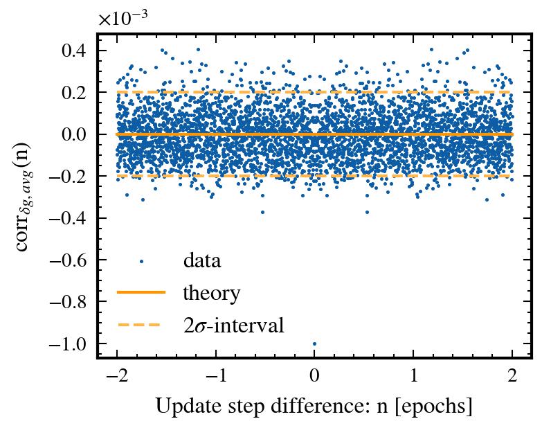
Figure 6: Autocorrelations of the SGDM noise compared for drawing examples without replacement (left) and with replacement (right).

Upon reviewing Fig. 7, it is clear that the velocity variance stays unchanged as predicted. However, while the weight variance remains constant for a broader subset of Hessian eigenvalues, it reduces for extremely small eigenvalues. Likewise, the correlation time is still limited for these minuscule Hessian eigenvalues. These deviations can be attributed to the finite time frame of the analysis period, comprising $2\cdot 10^{4}$ update steps. This limited time window sets a cap on the maximum correlation time, consequently leading to a decreased weight variance for these small Hessian eigenvalues. Despite this, it is noteworthy that this maximum correlation time is still roughly one order of magnitude longer than the maximum correlation time induced by the correlations arising from the epoch-based learning approach.

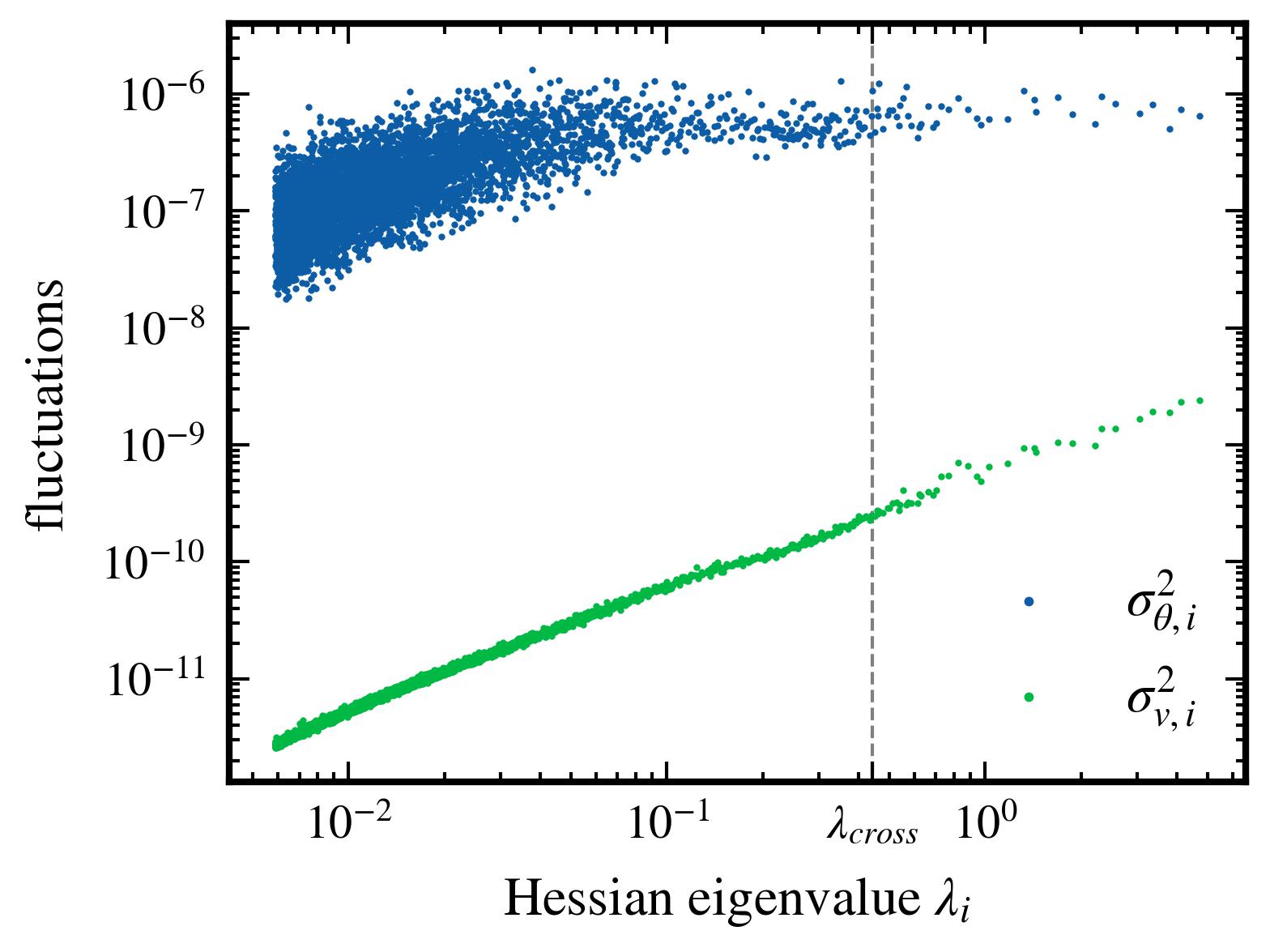
Figure 7: Relationship between Hessian eigenvalues and the variances of weights and velocities, as well as correlation times. For the left column the examples are drawn in epochs without replacement and for the right column the examples are drawn with replacement.

Appendix D Variance Calculation

D.1 Commutation of the covariance matrices

In this section, we show that if $\left[\bm{\mathbf{C}},\bm{\mathbf{H}}\right]=0$ also $\bm{\mathbf{\Sigma}}$ and $\bm{\mathbf{\Sigma_{v}}}$ will commute with $\bm{\mathbf{C}}$, with $\bm{\mathbf{H}}$ and with each other. We make the assumptions one to three from Sec. 4.3 and therefore the SGD update equations become

$$\vec{v}_{k} =-\eta\vec{H}\vec{\theta}_{k-1}+\beta\vec{v}_{k-1}-\eta\vec{\delta g}_{k}\ ,$$ (13)

$$\bm{\mathbf{\theta}}_{k} =\left(\vec{1}-\eta\vec{H}\right)\vec{\theta}_{k-1}+\beta\vec{v}_{k-1}-\eta\vec{\delta g}_{k}\ ,$$ (14)

which can be rewritten by using the vector $\vec{y}_{k}\coloneqq\bigl{(}\bm{\mathbf{\theta}}_{k}\quad\vec{v}_{k}\bigr{)}^{\top}$, combining both the current weight and velocity variable, to be

$$\vec{y}_{k+1}=\vec{X}\vec{y}_{k}-\vec{z}_{k+1}\ .$$ (15)

Here, $\vec{z}_{k}\coloneqq\bigl{(}\eta\vec{\delta g}_{k}\quad\eta\vec{\delta g}_{k}\bigr{)}^{\top}$ contains the current noise term, and the matrix governing the deterministic part of the update is defined to be

$$\vec{X}\coloneqq\begin{pmatrix}\vec{1}-\eta\vec{H}&\beta\vec{1}\\ -\eta\vec{H}&\beta\vec{1}\end{pmatrix}.$$ (16)

By iteratively applying Eq. 16 we obtain

$$\vec{y}_{k+h}=\vec{X}^{h}\vec{y}_{k}-\sum_{i=1}^{h}\vec{X}^{h-i}\vec{z}_{k+i}\ .$$ (17)

Under the assumption $0\leq\beta<1$ and $0<\eta\lambda_{i}<2(1+\beta)$, for all eigenvalues $\lambda_{i}$ of $\vec{H}$, the magnitude of the eigenvalues of $\bm{\mathbf{X}}$ will be less than one. It is straightforward to show this relation for the eigenvalues of $\vec{X}$ by using the eigenbasis of $\vec{H}$. Therefore,

$$\lim_{h\rightarrow\infty}\vec{X}^{h}\vec{y}_{k}=0.$$ (18)

As we can shift the index in the weight variance, $h$ can be chosen arbitrarily large, which yields the following relation for the covariance

$$\langle\vec{y}_{k}\vec{y}_{k}^{\top}\rangle=\lim_{h\rightarrow\infty}\sum_{i,j=1}^{h}\vec{X}^{h-i}\langle\vec{z}_{k+i}\vec{z}_{k+j}^{\top}\rangle\left(\vec{X}^{h-j}\right)^{\top}.$$ (19)

Because Eq. 18 implies $\langle\bm{\mathbf{y}}_{k}\rangle=0$ and therefore $\langle\vec{\theta}_{k}\rangle=0$ and $\langle\vec{v}_{k}\rangle=0$, the left hand side of Eq. 19 contains the covariance matrices of interest,

$$\langle\vec{y}_{k}\vec{y}_{k}^{\top}\rangle=\begin{pmatrix}\vec{\Sigma}&\langle\vec{\theta}_{k}\vec{v}_{k}^{\top}\rangle\\ \langle\vec{v}_{k}\vec{\theta}_{k}^{\top}\rangle&\vec{\Sigma_{v}}\end{pmatrix}.$$ (20)

From Eq. 19 we can also infer that $\langle\vec{y}_{k}\vec{y}_{k}^{\top}\rangle$ is finite as the magnitude of the eigenvalues of $\bm{\mathbf{X}}$ is less than one. Consequently, by Eq. 20, the covariance matrices $\bm{\mathbf{\Sigma}}$ and $\vec{\Sigma_{v}}$ are finite as well. The average over the noise terms $\vec{z}_{k}$ on the right hand side of Eq. 19 is by assumption equal to

$$\langle\vec{z}_{k+i}\vec{z}_{k+j}^{\top}\rangle=\eta^{2}\left(\delta_{i,j}-\mathbf{1}_{\{1,...,M\}}(|i-j|)\frac{M-|i-j|}{M(M-1)}\right)\cdot\begin{pmatrix}\vec{C}&\vec{C}\\ \vec{C}&\vec{C}\end{pmatrix},$$ (21)

from which it follows that for any finite $h$ every matrix entry of the two by two super matrix on the right hand side of Eq. 19 is a function of $\bm{\mathbf{C}}$ and $\bm{\mathbf{H}}$. Therefore, when considering the limit $h\rightarrow\infty$, $\left[\bm{\mathbf{C}},\bm{\mathbf{H}}\right]=0$ implies that $\vec{\Sigma}$ and $\vec{\Sigma_{v}}$ will also commute with $\bm{\mathbf{C}}$, with $\bm{\mathbf{H}}$ and with each other.

D.2 Proof of the variance formula for one specific eigenvalue

Since $\bm{\mathbf{\Sigma}}$ and $\bm{\mathbf{\Sigma_{v}}}$ will commute with $\bm{\mathbf{C}}$, with $\bm{\mathbf{H}}$ and with each other, it is sufficient to prove the one dimensional case. For the multidimensional case simply apply the proof in the direction of each common eigenvector individually. The expectation values discussed below are computed with respect to the asymptotic distributions of $\theta$ and $v$, since we are only interested in the asymptotic behavior of training. We want to find $\sigma_{\theta}^{2}\coloneqq\langle\theta_{k}\theta_{k}\rangle$ and $\sigma_{v}^{2}\coloneqq\langle v_{k}v_{k}\rangle$. We assume $0\leq\beta<1$ and $0<\eta\lambda<2(1+\beta)$ where $\lambda$ is the hessian eigenvalue.

The equations describing SGD in one dimension are:

$$g_{k}(\theta) =\frac{\partial}{\partial\theta}L(\theta)+\delta g_{k}(\theta)$$ (22)

$$v_{k} =-\eta g_{k}(\theta_{k-1})+\beta v_{k-1}$$ (23)

$$\theta_{k} =\theta_{k-1}+v_{k}$$ (24)

Our remaining assumptions can then be described the following way

$$L(\theta) =\frac{1}{2}\theta\lambda\theta$$ (25)

$$\delta g_{k}(\theta) =\delta g_{k}\textrm{ }\dots\textrm{ is independent of }\theta$$ (26)

$$\Rightarrow\langle\delta g_{k}\delta g_{k+h}\rangle =\sigma_{\delta g}^{2}\left(\delta_{h,0}-\mathbf{1}_{\{1,...,M\}}(|h|)\frac{M-|h|}{M(M-1)}\right)$$ (27)

$$\sigma_{\delta g}^{2} \coloneqq\langle\delta g_{k}\delta g_{k}\rangle.$$ (28)

With these assumptions the update equations can be described by a discrete stochastic linear equation of second order

$$\theta_{k}=(1+\beta-\eta\lambda)\theta_{k-1}-\beta\theta_{k-2}-\eta\delta g_{k}$$ (29)

which can be rewritten into matrix form as follows

$$\bm{\mathbf{x}}_{k} =\vec{D}\vec{x}_{k-1}-\eta\delta g_{k}\vec{e}_{1}$$ (30)

$$\bm{\mathbf{x}}_{k} \coloneqq\begin{pmatrix}\theta_{k}\\ \theta_{k-1}\end{pmatrix}$$ (31)

$$\bm{\mathbf{e}}_{1} \coloneqq\begin{pmatrix}1\\ 0\end{pmatrix}$$ (32)

$$\vec{D} \coloneqq\begin{pmatrix}1+\beta-\eta\lambda&-\beta\\ 1&0\end{pmatrix}.$$ (33)

We are now interested in the following covariance matrix

$$\vec{\Sigma} \coloneqq\left\langle\vec{x}_{k}\vec{x}_{k}^{\top}\right\rangle$$

$$=\begin{pmatrix}\sigma_{\theta}^{2}&\langle\theta_{k}\theta_{k-1}\rangle\\ \langle\theta_{k}\theta_{k-1}\rangle&\sigma_{\theta}^{2}\end{pmatrix}$$ (34)

where the second equality is due to the fact that $\langle\theta_{k}\theta_{k}\rangle=\langle\theta_{k-1}\theta_{k-1}\rangle$. As we are interested in the asymptotic covariance, this expectation value is independent of any finite shift of the index $k$. By inserting Eq. 30 into $\left\langle\vec{x}_{k}\vec{x}_{k}^{\top}\right\rangle$ we arrive at the following equality

$$\left\langle\vec{x}_{k}\vec{x}_{k}^{\top}\right\rangle=\vec{D}\left\langle\vec{x}_{k-1}\vec{x}_{k-1}^{\top}\right\rangle\vec{D}^{\top}+\eta^{2}\left\langle\delta g_{k}\delta g_{k}\right\rangle\vec{e}_{1}\vec{e}_{1}^{\top}-\eta\left(\vec{D}\left\langle\bm{\mathbf{x}}_{k-1}\delta g_{k}\right\rangle\vec{e}_{1}^{\top}+\left(\vec{D}\left\langle\bm{\mathbf{x}}_{k-1}\delta g_{k}\right\rangle\vec{e}_{1}^{\top}\right)^{\top}\right)$$ (35)

which can be simplified to the equivalent equation

$$\vec{\Sigma}-\vec{D}\vec{\Sigma}\vec{D}^{\top}=\eta^{2}\sigma_{\delta g}^{2}\vec{e}_{1}\vec{e}_{1}^{\top}-\eta\left(\vec{D}\left\langle\bm{\mathbf{x}}_{k-1}\delta g_{k}\right\rangle\vec{e}_{1}^{\top}+\left(\vec{D}\left\langle\bm{\mathbf{x}}_{k-1}\delta g_{k}\right\rangle\vec{e}_{1}^{\top}\right)^{\top}\right).$$ (36)

If we apply the left-hand side on the vector $\vec{e}_{1}$, it can be expressed as

$$\left[\vec{\Sigma}-\vec{D}\vec{\Sigma}\vec{D}^{\top}\right]\vec{e}_{1} =\vec{F}_{1}^{-1}\vec{\Sigma}\vec{e}_{1}$$ (37)

$$\vec{F}_{1}^{-1} \coloneqq\begin{pmatrix}\eta\lambda(2-\eta\lambda)-2\beta(1+\beta-\eta\lambda)&2\beta(1+\beta-\eta\lambda)\\ -(1+\beta-\eta\lambda)&1+\beta\end{pmatrix}.$$ (38)

Also notice $v_{k}=\theta_{k}-\theta_{k-1}$ and therefore

$$\sigma_{v}^{2}=2\sigma_{\theta}^{2}-2\langle\theta_{k}\theta_{k-1}\rangle,$$ (39)

again due to the fact that the expectation value does not depend on k. Hence, the variances can then be expressed as

$$\begin{pmatrix}\sigma_{\theta}^{2}\\ \sigma_{v}^{2}\end{pmatrix} =\vec{F}_{2}\vec{\Sigma}\vec{e}_{1}$$ (40)

$$\vec{F}_{2} \coloneqq\begin{pmatrix}1&0\\ 2&-2\end{pmatrix}.$$ (41)

We define the matrix $\vec{F}\coloneqq\vec{F}_{2}\vec{F}_{1}$. By applying both sides of Eq. 36 to the vector $\vec{e_{1}}$, then multiplying by the matrix $\vec{F}$ from the left and using Eqs. 37 and 40 we obtain

$$\begin{pmatrix}\sigma_{\theta}^{2}\\ \sigma_{v}^{2}\end{pmatrix}=\vec{F}\left[\eta^{2}\sigma_{\delta g}^{2}\vec{e}_{1}\vec{e}_{1}^{\top}-\eta\left(\vec{D}\left\langle\bm{\mathbf{x}}_{k-1}\delta g_{k}\right\rangle\vec{e}_{1}^{\top}+\left(\vec{D}\left\langle\bm{\mathbf{x}}_{k-1}\delta g_{k}\right\rangle\vec{e}_{1}^{\top}\right)^{\top}\right)\right]\vec{e}_{1}\ .$$ (42)

with

$$\bm{\mathbf{F}}=\frac{1}{(1-\beta)\bigl{(}2(1+\beta)-\eta\lambda)\bigr{)}}\begin{pmatrix}\frac{1+\beta}{\eta\lambda}&\frac{2\beta(\eta\lambda-1-\beta)}{\eta\lambda}\\ 2&2(\eta\lambda-2)\end{pmatrix}.$$ (43)

To simplify Eq. 42 further we go back to Eq. 30 and iterate it to obtain

$$\bm{\mathbf{x}}_{k}=\vec{D}^{n}\bm{\mathbf{x}}_{k-n}-\eta\sum_{h=0}^{n-1}\vec{D}^{h}\vec{e}_{1}\delta g_{k-h}\ .$$ (44)

We note that $\left\langle\bm{\mathbf{x}}_{k-n}\delta g_{k}\right\rangle=0$ for $n\geq M$. The correlation between noise terms separated by at least one epoch vanishes, and $\bm{\mathbf{x}}_{k}$ only depends on past noise terms. By setting $n=M$ we find

$$\left\langle\bm{\mathbf{x}}_{k-1}\delta g_{k}\right\rangle =\vec{D}^{M}\left\langle\bm{\mathbf{x}}_{k-1-M}\delta g_{k}\right\rangle-\eta\sum_{h=0}^{M-1}\vec{D}^{h}\vec{e}_{1}\left\langle\delta g_{k}\delta g_{k-1-h}\right\rangle$$

$$=-\eta\sigma_{\delta g}^{2}\sum_{h=0}^{M-1}\vec{D}^{h}\vec{e}_{1}\left(-\frac{M-(h+1)}{M(M-1)}\right)\ ,$$ (45)

where the assumption about the correlation of the noise terms (Eq. 27) was inserted for the last line. Eq. 45 is a sum of a finite geometric series and a derivative of that which can be simplified to

$$\left\langle\bm{\mathbf{x}}_{k-1}\delta g_{k}\right\rangle =\eta\sigma_{\delta g}^{2}\frac{\bm{\mathbf{D}}^{M}+(\vec{1}-\vec{D})M-\vec{1}}{(\vec{1}-\vec{D})^{2}M(M-1)}\,\vec{e}_{1}.$$ (46)

Substituting this result back into Eq. 42 yields

$$\begin{pmatrix}\sigma_{\theta}^{2}\\ \sigma_{v}^{2}\end{pmatrix} =\eta^{2}\sigma_{\delta g}^{2}\vec{F}\left[\vec{e}_{1}-\left(\bm{\mathbf{E}}+\vec{E}^{\top}\right)\vec{e}_{1}\right]$$ (47)

with the definition

$$\vec{E} \coloneqq\vec{D}\frac{\bm{\mathbf{D}}^{M}+(\vec{1}-\vec{D})M-\vec{1}}{(\vec{1}-\vec{D})^{2}M(M-1)}\,\vec{e}_{1}\vec{e}_{1}^{\top}\ .$$ (48)

With Eq. 47 we have arrived at the exact formula for the variances which can easily be evaluated numerically.

D.3 Approximation of the exact formula

It is possible to approximate the exact result for the variance assuming small or large eigenvalues, respectively. For that, it is necessary to approximate $\bm{\mathbf{D}}^{M}\bm{\mathbf{e_{1}}}$. To do so, we will use the the following eigendecomposition of $\bm{\mathbf{D}}$

$$\vec{D} =\vec{Q}\vec{\Lambda}\vec{Q}^{-1}$$ (49)

$$\vec{\Lambda} =\begin{pmatrix}\Lambda_{+}&0\\ 0&\Lambda_{-}\end{pmatrix}$$ (50)

$$\vec{Q} =\begin{pmatrix}\Lambda_{+}&\Lambda_{-}\\ 1&1\end{pmatrix}$$ (51)

$$\vec{Q}^{-1} =\frac{1}{\Lambda_{+}-\Lambda_{-}}\begin{pmatrix}1&-\Lambda_{-}\\ -1&\Lambda_{+}\end{pmatrix}$$ (52)

$$\Lambda_{\pm} =\frac{1}{2}\left(1+\beta-\eta\lambda\pm s\right)$$ (53)

$$s \coloneqq\sqrt{\left(1-\beta\right)^{2}-\eta\lambda\bigl{(}2(1+\beta)-\eta\lambda\bigr{)}}$$ (54)

It is straightforward to show that the magnitude of the eigenvalues of $\vec{D}$ is strictly smaller than one, $|\Lambda_{\pm}|<1$, under the conditions $0<\eta\lambda<2(1+\beta)$ and $0\leq\beta<1$.

Large hessian eigenvalues

$$\sigma_{\theta}^{2} \approx\frac{\eta^{2}\sigma_{\delta g}^{2}}{(1-\beta)(2(1+\beta)-\eta\lambda)}\cdot\frac{1+\beta}{\eta\lambda}$$ (55)

$$\sigma_{v}^{2} \approx\frac{\eta^{2}\sigma_{\delta g}^{2}}{(1-\beta)(2(1+\beta)-\eta\lambda)}\cdot 2$$ (56)

We will show that this approximation for large hessian eigenvalues is valid under the assumption $M(\eta\lambda)^{2}\gg 1$ where $M$ is the number of batches per epoch. However, numerical studies indicate that these relations also hold under the previously mentioned assumptions of $\frac{M\eta\lambda}{1-\beta}\gg 1$, equivalent to $\lambda\gtrsim\lambda_{\textrm{cross}}$, and $M(1-\beta)\gg 1$.

Inserting the eigendecomposition of $\bm{\mathbf{D}}$ into the expression $\vec{D}^{M}\vec{e_{1}}$ yields

$$\vec{D}^{M}\vec{e_{1}}=\begin{pmatrix}y_{M+1}\\ y_{M}\end{pmatrix}$$ (57)

$$y_{M}\coloneqq\frac{\Lambda_{+}^{M}-\Lambda_{-}^{M}}{\Lambda_{+}-\Lambda_{-}}.$$ (58)

From the definition of $y_{M}$ one sees that

$$y_{M}=\frac{\Lambda_{+}+\Lambda_{-}}{2}\,y_{M-1}+\frac{\Lambda_{+}^{M-1}+\Lambda_{-}^{M-1}}{2}\ ,$$ (59)

and by using $|\Lambda_{\pm}|<1$ as well as $y_{0}=0$ one can show iteratively that

$$|y_{M}|\leq M+1.$$ (60)

Therefore, we have

$$\left\lVert\vec{D}^{M}\vec{e_{1}}\right\rVert_{\infty}\leq M+1$$ (61)

where $\left\lVert\cdot\right\rVert_{\infty}$ is denoting the maximum norm $\left\lVert\bm{\mathbf{x}}\right\rVert_{\infty}\coloneqq\max_{i}|x_{i}|$ for a vector $\vec{x}$ or its induced matrix norm $\left\lVert\bm{\mathbf{A}}\right\rVert_{\infty}\coloneqq\max_{i}\sum_{j}|a_{ij}|$ for a matrix $\vec{A}$.

Explicit calculations show that

$$\left\lVert(\bm{\mathbf{1}}-\vec{D})^{-1}\right\rVert_{\infty}\leq\frac{4}{\eta\lambda}$$ (62)

under the assumption that $0\leq\beta<1$ and $0<\eta\lambda<2(1+\beta)$. From here it is straightforward to show that

$$\left\lVert\left(\vec{E}+\vec{E}^{\top}\right)\vec{e_{1}}\right\rVert_{\infty}\leq\frac{\tilde{c}}{M(\eta\lambda)^{2}}$$ (63)

where $\tilde{c}$ is a factor of order unity under the constraints $0\leq\beta<1$ and $0<\eta\lambda<2(1+\beta)$. By substituting this result back into Eq. 47 one directly sees that a comparison to the approximation yields

$$\left\lvert 1-\frac{\sigma_{\theta}^{2}}{\sigma_{\theta,\textrm{large}}^{2}}\right\rvert\leq\frac{c_{1}}{M(\eta\lambda)^{2}}\ ,$$ (64)

$$\left\lvert 1-\frac{\sigma_{v}^{2}}{\sigma_{v,\textrm{large}}^{2}}\right\rvert\leq\frac{c_{2}}{M(\eta\lambda)^{2}}\ ,$$ (65)

where $c_{1}$ and $c_{2}$ are again of order unity and the approximation is defined as

$$\begin{pmatrix}\sigma_{\theta,\textrm{large}}^{2}\\ \sigma_{v,\textrm{large}}^{2}\end{pmatrix} \coloneqq\eta^{2}\sigma_{\delta g}^{2}\vec{F}\vec{e}_{1}$$

$$=\frac{\eta^{2}\sigma_{\delta g}^{2}}{(1-\beta)(2(1+\beta)-\eta\lambda)}\cdot\begin{pmatrix}\frac{1+\beta}{\eta\lambda}\\ 2\end{pmatrix}.$$ (66)

Interestingly, one can see that the approximation for large hessian eigenvalues is equivalent to the result we would obtain if we assumed there was no autocorrelation of the noise to begin with.

In the case where the stricter assumption is not true, $M(\eta\lambda)^{2}<1$, but the numerically obtained conditions still hold, $\lambda\gtrsim\lambda_{\textrm{cross}}$ and $M(1-\beta)\gg 1$, it occurs that $\left\lVert\left(\vec{E}+\vec{E}^{\top}\right)\vec{e_{1}}\right\rVert_{\infty}$ is no longer small. But in that case, $\vec{F}\left(\vec{E}+\vec{E}^{\top}\right)\vec{e_{1}}$ can still be neglected compared to $\vec{F}\vec{e_{1}}$, as numerical experiments show.

Small hessian eigenvalues

To obtain the relations for small hessian eigenvalues, we perform a Taylor expansion with respect to $\lambda$ with the help of computer algebra. We neglect the terms which are at least of order lambda. Numerical study indicates that these relations hold under the mentioned assumption of $\lambda\lesssim\lambda_{\textrm{cross}}$ and $M(1-\beta)\gg 1$.

It is straightforward but lengthy to obtain the following expression using the eigendecomposition of $\vec{D}$

$$\begin{pmatrix}\sigma_{\theta}^{2}\\ \sigma_{v}^{2}\end{pmatrix}=\frac{\eta^{2}\sigma_{\delta g}^{2}}{2(1-\beta)(1+\beta)}\cdot\begin{pmatrix}\frac{M}{3}\frac{1+\beta}{1-\beta}+\mathcal{O}(\lambda)\\ 2+\mathcal{O}(\lambda)\end{pmatrix}$$ (67)

where the zeroth order terms are simplified under approximation $M(1-\beta)\gg 1$.

D.4 Satisfying the assumptions of the correlation time relation

In this section we want to show that the weight and velocity variances resulting from stochastic gradient descent as described above and in Sec. 4.3 satisfies the necessary assumptions (i) to (iv) of Sec. 4.2 such that the velocity correlation time is equal to $\tau_{i}=2\sigma_{\theta,i}^{2}/\sigma_{v,i}^{2}$. Validity of assumption (i) existence and finiteness of $\bm{\mathbf{\Sigma}}\coloneqq$ cov$(\bm{\mathbf{\theta}}_{k},\bm{\mathbf{\theta}}_{k})$, $\bm{\mathbf{\Sigma_{v}}}\coloneqq$ cov$(\bm{\mathbf{v}}_{k},\bm{\mathbf{v}}_{k})$, and $\langle\bm{\mathbf{\theta}}\rangle$, and assumption (ii), $[\bm{\mathbf{\Sigma}},\bm{\mathbf{\Sigma_{v}}}]=0$, can be inferred from the calculation presented in Appendix D.1. Therefore, we concentrate on assumption (iii) $\lim_{n\to\infty}\textrm{cov}\bigr{(}\bm{\mathbf{\theta}}_{k},\bm{\mathbf{\theta}}_{k+n}\bigr{)}=0$ and (iv) $\lim_{n\to\infty}n\cdot\textrm{cov}\bigr{(}\bm{\mathbf{\theta}}_{k},\bm{\mathbf{\theta}}_{k+n}-\bm{\mathbf{\theta}}_{k+n+1}\bigr{)}=0$. Since $\left[\bm{\mathbf{\Sigma_{\theta}}},\bm{\mathbf{\Sigma_{v}}}\right]=0$, it is sufficient to consider the one dimensional case. Additionally $\langle\vec{\theta}\rangle=0$ (Appendix D.1) and, therefore, the remaining two assumptions (iii) and (iv) can be written as $\lim_{m\rightarrow\infty}{\langle\theta_{k}\theta_{k+m}\rangle}=0$ and $\lim_{m\rightarrow\infty}{m\bigl{(}\langle\theta_{k}\theta_{k+m}\rangle-\langle\theta_{k}\theta_{k+m+1}\rangle\bigr{)}}=0$.

We will now show that for stochastic gradient descent under the assumptions of Sec. 4.3 the more restrictive relation $\lim_{m\rightarrow\infty}{m\langle\theta_{k}\theta_{k+m}\rangle}=0$ is satisfied, from which follows (iii) and (iv). Following Appendix D.2 and using the same notation, we have the relation

$$\langle\vec{x}_{k}\vec{x}_{k-m}^{\top}\rangle=\bm{\mathbf{D}}\langle\vec{x}_{k-1}\vec{x}_{k-m}^{\top}\rangle-\eta\vec{e_{1}}\langle\delta g_{k}\vec{x}_{k-m}^{\top}\rangle\ ,$$ (68)

where $\vec{x}_{k}\coloneqq\bigl{(}\theta_{k}\quad\theta_{k-1}\bigr{)}^{\top}$. For $m>M$, with $M$ being the number of batches per epoch, the correlation with the noise term on the right hand side of Eq. 68 is equal to zero as discussed in Appendix D.2. By iterating Eq. 68, for $m>M$ we have

$$\langle\vec{x}_{k}\vec{x}_{k-m}^{\top}\rangle =\bm{\mathbf{D}}^{m-M-1}\langle\vec{x}_{k-m+M+1}\vec{x}_{k-m}^{\top}\rangle$$

$$=\bm{\mathbf{D}}^{m-M-1}\langle\vec{x}_{k}\vec{x}_{k-M-1}^{\top}\rangle\ .$$ (69)

As described in Appendix D.2, the magnitude of both eigenvalues of $\vec{D}$ is strictly smaller than one. This implies that there exists a matrix norm $\left\lVert\cdot\right\rVert_{\vec{D}}$ such that $\left\lVert\vec{D}\right\rVert_{\vec{D}}<1$ from which one can deduce

$$m\left\lVert\langle\vec{x}_{k}\vec{x}_{k-m}^{\top}\rangle\right\rVert_{\vec{D}}\leq\left\lVert\bm{\mathbf{D}}\right\rVert_{\vec{D}}^{m-M-1}\cdot\left\lVert\langle\vec{x}_{k}\vec{x}_{k-M-1}^{\top}\rangle\right\rVert_{\vec{D}}\ .$$ (70)

Taking the limit of $m\to\infty$ we obtain

$$\lim_{m\to\infty}m\left\lVert\langle\vec{x}_{k}\vec{x}_{k-m}^{\top}\rangle\right\rVert_{\vec{D}} \leq\textrm{const}\cdot\lim_{m\to\infty}\left\lVert\bm{\mathbf{D}}\right\rVert_{\vec{D}}^{m-M-1}$$

$$=0\ ,$$ (71)

and because

$$\langle\vec{x}_{k}\vec{x}_{k-m}^{\top}\rangle=\begin{pmatrix}\langle\theta_{k}\theta_{k-m}\rangle&\langle\theta_{k}\theta_{k-m-1}\rangle\\ \langle\theta_{k-1}\theta_{k-m}\rangle&\langle\theta_{k-1}\theta_{k-m-1}\rangle\end{pmatrix}$$ (72)

we finally find

$$\lim_{m\rightarrow\infty}{m\langle\theta_{k}\theta_{k-m}\rangle} =0$$

$$\Rightarrow\lim_{m\rightarrow\infty}{m\langle\theta_{k}\theta_{k+m}\rangle} =0\ .$$ (73)

Appendix E Calculation of the correlation time relation

We want to prove the relation

$$\frac{2\sigma_{\theta,i}^{2}}{\sigma_{v,i}^{2}}=\frac{\sum_{n=1}^{\infty}n\,\langle v_{k,i}v_{k+n,i}\rangle}{\sum_{n=1}^{\infty}\langle v_{k,i}v_{k+n,i}\rangle}\ .$$ (74)

We assume that that $\langle\vec{\theta}\rangle$, $\bm{\mathbf{\Sigma_{\theta}}}$ and $\bm{\mathbf{\Sigma_{v}}}$ exist and are finite. Without loss of generality, let $\langle\vec{\theta}\rangle=0$. We further assume that $\left[\bm{\mathbf{\Sigma_{\theta}}},\bm{\mathbf{\Sigma_{v}}}\right]=0$. Therefore, it is sufficient to consider the one-dimensional case. For the multidimensional case, simply apply the proof in the direction of each common eigenvector individually. The remaining two assumptions (iii) and (iv) of Sec. 4.2 can now be written as

$$\lim\limits_{m\rightarrow\infty}{\langle\theta_{k}\theta_{k+m}\rangle} =0$$ (75)

$$\lim\limits_{m\rightarrow\infty}{m\bigl{(}\langle\theta_{k}\theta_{k+m}\rangle-\langle\theta_{k}\theta_{k+m+1}\rangle\bigr{)}} =0\ .$$ (76)

We begin the proof with the following chain of equations

$$\sigma_{\theta}^{2} =\left\langle\theta_{k}^{2}\right\rangle$$

$$=\left\langle\left(\theta_{k}-\theta_{k+J}+\theta_{k+J}\right)^{2}\right\rangle$$

$$=\left\langle\left(\theta_{k}-\theta_{k+J}\right)^{2}\right\rangle-2\left\langle\theta_{k+J}^{2}\right\rangle+2\left\langle\theta_{k}\theta_{k+J}\right\rangle+\left\langle\theta_{k+J}^{2}\right\rangle\ ,$$ (77)

which holds for any integer $J$. We have $\left\langle\theta_{k+J}^{2}\right\rangle=\left\langle\theta_{k}^{2}\right\rangle$ since the expectation value cannot depend on $k$. Additionally, by definition we have $v_{k}=\theta_{k}-\theta_{k-1}$ which yields

$$\theta_{k}-\theta_{k+J}=\sum_{i=1}^{J}v_{k+i}\ .$$ (78)

Therefore, we can rewrite Eq. 77 as follows

$$2\sigma_{\theta}^{2} =2\left\langle\theta_{k}\theta_{k+J}\right\rangle+\sum_{i,j=1}^{J}\langle v_{k+i}v_{k+j}\rangle$$

$$=2\left\langle\theta_{k}\theta_{k+J}\right\rangle+\sum_{i,j=1}^{J}\langle v_{k}v_{k+j-i}\rangle$$

$$=2\left\langle\theta_{k}\theta_{k+J}\right\rangle+\sum_{m=0}^{J-1}\sum_{n=-m}^{m}\langle v_{k}v_{k+n}\rangle\ ,$$ (79)

where we first shifted the index within the expectation value and then restructured the sum by defining $m\coloneqq\max(i,j)-1$ and $n\coloneqq j-i$. We now take the limit of $J\rightarrow\infty$ and because of Eq. 75 and the assumption of a finite $\sigma_{\theta}^{2}$ we have

$$\sum_{m=0}^{\infty}\sum_{n=-m}^{m}\langle v_{k}v_{k+n}\rangle <\infty$$ (80)

$$\Rightarrow\sum_{n=-\infty}^{\infty}\langle v_{k}v_{k+n}\rangle =0\ .$$ (81)

We note that $\langle v_{k}v_{k+n}\rangle=\langle v_{k}v_{k-n}\rangle$ because we can shift the index, and the two factors commute. Substituting this relation into Eq. 81 yields

$$\sum_{n=1}^{\infty}\langle v_{k}v_{k+n}\rangle =-\frac{1}{2}\langle v_{k}v_{k}\rangle$$

$$=-\frac{1}{2}\sigma_{v}^{2}\ .$$ (82)

For the second part of the proof we will start again with $v_{k}=\theta_{k}-\theta_{k-1}$ and the following sum

$$\sum_{n=1}^{m}n\langle v_{k}v_{k+n}\rangle =\sum_{n=1}^{m}n\bigl{(}2\langle\theta_{k}\theta_{k+n}\rangle-\langle\theta_{k-1}\theta_{k+n}\rangle-\langle\theta_{k}\theta_{k+n-1}\rangle\bigr{)}$$

$$=-\langle\theta_{k}\theta_{k}\rangle+\langle\theta_{k}\theta_{k+m}\rangle+m\bigl{(}\langle\theta_{k}\theta_{k+m}\rangle-\langle\theta_{k}\theta_{k+m+1}\rangle\bigr{)}\ ,$$ (83)

where nearly all terms cancel each other again due to the fact that we can shift the index within the expectation value. By taking the limit $m\rightarrow\infty$ and using the assumptions (iii) and (iv) (Eqs. 75 and 76) we have

$$\sum_{n=1}^{\infty}n\langle v_{k}v_{k+n}\rangle=-\langle\theta_{k}\theta_{k}\rangle\ .$$ (84)

Finally, by dividing Eq. 84 by Eq. 82 we arrive at the final expression

$$\frac{2\sigma_{\theta,i}^{2}}{\sigma_{v,i}^{2}}=\frac{\sum_{n=1}^{\infty}n\,\langle v_{k}v_{k+n}\rangle}{\sum_{n=1}^{\infty}\langle v_{k}v_{k+n}\rangle}\ .$$ (85)

Appendix F Calculation of the noise autocorrelation

We want to calculate the autocorrelation function of epoch-based SGD for a fixed weight vector $\bm{\mathbf{\theta}}$ and under the assumption that the total number of examples is an integer multiple of the number of examples per batch. For that we repeat the following definitions:

$$\bm{\mathbf{\delta g}}_{k}(\bm{\mathbf{\theta}}) \coloneqq\frac{1}{S}\sum_{n\in\mathcal{B}_{k}}\bm{\mathbf{\nabla}}\bigl{(}l(\bm{\mathbf{\theta}},x_{n})-L(\bm{\mathbf{\theta}})\bigr{)}$$ (86)

$$\mathcal{B}_{k}=\{n_{1},...,n_{S}\} \dots\text{ batch of step k, sampeling without replacement within epoch}$$ (87)

$$n_{j}\in\{1,\dots,N\}$$ (88)

$$N \dots\text{ total number of examples}$$ (89)

$$S \dots\text{ number of examples per batch}$$ (90)

We can rewrite the noise terms as follows:

$$\bm{\mathbf{\delta g}}_{k}(\bm{\mathbf{\theta}}) =\frac{1}{S}\sum_{n\in\mathcal{B}_{k}}\bm{\mathbf{\delta g_{e}}}(n,\bm{\mathbf{\theta}})$$

$$=\frac{1}{S}\sum_{n=1}^{N}\bm{\mathbf{\delta g_{e}}}(n,\bm{\mathbf{\theta}})s_{k}^{n}$$ (91)

$$s_{k}^{n} \coloneqq\mathbf{1}_{\mathcal{B}_{k}}(n)$$

$$=\begin{cases}1\ \text{ if }~{}n\in\mathcal{B}_{k}\\ 0\ \text{ if }~{}n\notin\mathcal{B}_{k}\end{cases}$$ (92)

$$\bm{\mathbf{\delta g_{e}}}(n,\bm{\mathbf{\theta}}) \coloneqq\bm{\mathbf{\nabla}}\bigl{(}l(\bm{\mathbf{\theta}},x_{n})-L(\bm{\mathbf{\theta}})\bigr{)}\ .$$ (93)

Let $h\geq 0$ be fixed. The correlation matrix can be expressed as

$$\textrm{cov}\bigl{(}\vec{\delta g}_{k}(\vec{\theta}),\vec{\delta g}_{k+h}(\vec{\theta})\bigr{)} =\mathbb{E}\left[\bm{\mathbf{\delta g}}_{k}(\bm{\mathbf{\theta}})\bm{\mathbf{\delta g}}_{k+h}(\bm{\mathbf{\theta}})^{\top}\right]$$

$$=\frac{1}{S^{2}}\sum_{n,\tilde{n}=1}^{N}\bm{\mathbf{\delta g_{e}}}(n,\bm{\mathbf{\theta}})\bm{\mathbf{\delta g_{e}}}(\tilde{n},\bm{\mathbf{\theta}})^{\top}\mathbb{E}\left[s_{k}^{n}s_{k+h}^{\tilde{n}}\right]\ .$$ (94)

The expectation value of $s_{k}^{n}=\mathbf{1}_{\mathcal{B}_{k}}(n)$ is the probability that example $n$ is part of batch $k$. Because every example is equally likely to appear in a given batch, this probability is equal to $S/N$.

$$\mathbb{E}\left[s_{k}^{n}\right] =\textrm{P}\!\left(s_{k}^{n}=1\right)$$

$$=\frac{S}{N}\ .$$ (95)

Similarly we can calculate the desired correlation:

$$\mathbb{E}\left[s_{k}^{n}s_{k+h}^{\tilde{n}}\right] =\textrm{P}\!\left(s_{k}^{n}=1,s_{k+h}^{\tilde{n}}=1\right)$$

$$=\textrm{P}\!\left(s_{k}^{n}=1\right)\textrm{P}\!\left(s_{k+h}^{\tilde{n}}=1\mid s_{k}^{n}=1\right)$$

$$=\frac{S}{N}\,\textrm{P}\!\left(s_{k+h}^{\tilde{n}}=1\mid s_{k}^{n}=1\right)\ .$$ (96)

The last term can be split up into different probabilities for different values of h. We can also distinguish the case where the two steps $k$ and $k+h$ are within the same epoch ($\textrm{ep}(k)=\textrm{ep}(k+h)$) or in different epochs ($\textrm{ep}(k)\neq\textrm{ep}(k+h)$).

$$\textrm{P}\!\left(s_{k+h}^{\tilde{n}}=1\mid s_{k}^{n}=1\right) =\delta_{h,0}\cdot\textrm{P}\!\left(s_{k}^{\tilde{n}}=1\mid s_{k}^{n}=1\right)+(1-\delta_{h,0})\,\cdot$$

$$\quad\Bigl{[}\textrm{P}\bigl{(}\textrm{ep}(k)=\textrm{ep}(k+h)\bigr{)}\textrm{P}\!\left(s_{k+h}^{\tilde{n}}=1\mid s_{k}^{n}=1,\textrm{ep}(k)=\textrm{ep}(k+h)\right)+$$

$$\quad\ \textrm{P}\bigl{(}\textrm{ep}(k)\neq\textrm{ep}(k+h)\bigr{)}\textrm{P}\!\left(s_{k+h}^{\tilde{n}}=1\mid s_{k}^{n}=1,\textrm{ep}(k)\neq\textrm{ep}(k+h)\right)\Bigr{]}\ .$$ (97)

The first term of the RHS of Eq. 97 is the probability that a given example occurs in a batch, assuming that we already know one of the examples of that batch.

$$\textrm{P}\!\left(s_{k}^{\tilde{n}}=1\mid s_{k}^{n}=1\right) =\textrm{P}\!\left(s_{k}^{n}=1\mid s_{k}^{n}=1\right)\cdot\,\delta_{n,\tilde{n}}+\textrm{P}\!\left(s_{k}^{\tilde{n}}=1\mid s_{k}^{n}=1,n\neq\tilde{n}\right)\,(1-\delta_{n,\tilde{n}})$$

$$=1\cdot\,\delta_{n,\tilde{n}}+\frac{S-1}{N-1}\,(1-\delta_{n,\tilde{n}})$$

$$=\frac{N-S}{N-1}\,\delta_{n,\tilde{n}}+\textrm{const.}$$ (98)

The second term of Eq. 97 is multiplied by $(1-\delta_{h,0})$. Therefore, we assume $h\geq 1$ for the following argument. That is, we want to know the probabilities under the assumption that we are comparing examples from different batches. If the two batches are still from the same epoch, examples cannot repeat as the total number of examples is an integer multiple of the number of examples per batch and because of that every example is shown only once per epoch. Therefore, for $h\geq 1$ holds:

$$\textrm{P}\!\left(s_{k+h}^{\tilde{n}}=1\mid s_{k}^{n}=1,\textrm{ep}(k)=\textrm{ep}(k+h)\right) =0\cdot\delta_{n,\tilde{n}}+\frac{S}{N-1}\,(1-\delta_{n,\tilde{n}})$$

$$=-\frac{S}{N-1}\delta_{n,\tilde{n}}+\textrm{const.}$$ (99)

If we consider batches from different epochs, the probability becomes independent of the given examples:

$$\textrm{P}\!\left(s_{k+h}^{\tilde{n}}=1\mid s_{k}^{n}=1,\textrm{ep}(k)\neq\textrm{ep}(k+h)\right) =\frac{S}{N}$$

$$=\textrm{const.}$$ (100)

Lastly, we need to know the probability that two given batches $k$ and $k+h$ are from the same epoch:

$$\textrm{P}\bigl{(}\textrm{ep}(k)=\textrm{ep}(k+h)\bigr{)}=\mathbf{1}_{\{1,\dots,M\}}(h)\,\frac{M-h}{M}\ ,$$ (101)

where $M=N/S$ is again the number of batches per epoch.

We can now combine all derived probabilities and arrive at the following relation:

$$\mathbb{E}\left[s_{k}^{n}s_{k+h}^{\tilde{n}}\right] =\delta_{n,\tilde{n}}\,\frac{S}{N}\frac{N-S}{N-1}\left(\delta_{h,0}-\mathbf{1}_{\{1,\dots,M\}}(h)\frac{S}{N-S}\frac{M-h}{M}\right)+\textrm{const.}$$

$$=\delta_{n,\tilde{n}}\,S^{2}\left(\frac{1}{S}-\frac{1}{N}\right)\frac{}{}\frac{1}{N-1}\left(\delta_{h,0}-\mathbf{1}_{\{1,\dots,M\}}(h)\frac{M-h}{M\,(M-1)}\right)+\textrm{const.}$$ (102)

If we now also consider negative values for h, the expression depends only on the absolute value of h due to symmetry.

By using the following two helpful relations:

$$\sum_{n,\tilde{n}=1}^{N}\bm{\mathbf{\delta g_{e}}}(n,\bm{\mathbf{\theta}})\bm{\mathbf{\delta g_{e}}}(\tilde{n},\bm{\mathbf{\theta}})^{\top}\,\delta_{n,\tilde{n}} =\sum_{n=1}^{N}\bm{\mathbf{\delta g_{e}}}(n,\bm{\mathbf{\theta}})\bm{\mathbf{\delta g_{e}}}(n,\bm{\mathbf{\theta}})^{\top}$$

$$\eqqcolon(N-1)\,\bm{\mathbf{C}}_{0}(\bm{\mathbf{\theta}})\ ,$$ (103)

$$\sum_{n,\tilde{n}=1}^{N}\bm{\mathbf{\delta g_{e}}}(n,\bm{\mathbf{\theta}})\bm{\mathbf{\delta g_{e}}}(\tilde{n},\bm{\mathbf{\theta}})^{\top}\cdot 1 =\left(\sum_{n=1}^{N}\bm{\mathbf{\delta g_{e}}}(n,\bm{\mathbf{\theta}})\right)\left(\sum_{n=1}^{N}\bm{\mathbf{\delta g_{e}}}(n,\bm{\mathbf{\theta}})^{\top}\right)$$

$$=\bm{\mathbf{\nabla}}\bigl{(}L(\bm{\mathbf{\theta}})-L(\bm{\mathbf{\theta}})\bigr{)}\bm{\mathbf{\nabla}}^{\top}\bigl{(}L(\bm{\mathbf{\theta}})-L(\bm{\mathbf{\theta}})\bigr{)}$$

$$=0\ ,$$ (104)

we can insert the expectation value $\mathbb{E}\left[s_{k}^{n}s_{k+h}^{\tilde{n}}\right]$ into Eq. 94 and arrive at the final expression:

$$\textrm{cov}\bigl{[}\vec{\delta g}_{k}(\vec{\theta}),\vec{\delta g}_{k+h}(\vec{\theta})\bigr{]} =\textrm{cov}\bigl{[}\vec{\delta g}_{k}(\vec{\theta}),\vec{\delta g}_{k}(\vec{\theta})\bigr{]}\cdot\left(\delta_{h,0}-\mathbf{1}_{\{1,...,M\}}(|h|)\frac{M-|h|}{M(M-1)}\right),$$ (105)

$$\textrm{cov}\bigl{[}\vec{\delta g}_{k}(\vec{\theta}),\vec{\delta g}_{k}(\vec{\theta})\bigr{]} =\left(\frac{1}{S}-\frac{1}{N}\right)\bm{\mathbf{C}}_{0}(\bm{\mathbf{\theta}})\ .$$ (106)

References

- Bottou [1991] Léon Bottou. Stochastic gradient learning in neural networks. Proceedings of Neuro-Nımes, 91(8):12, 1991.
- LeCun et al. [2015] Yann LeCun, Yoshua Bengio, and Geoffrey Hinton. Deep learning. Nature, 521(7553):436–444, May 2015. doi: 10.1038/nature14539. URL https://doi.org/10.1038/nature14539.
- Krizhevsky et al. [2012] Alex Krizhevsky, Ilya Sutskever, and Geoffrey E Hinton. Imagenet classification with deep convolutional neural networks. In Advances in Neural Information Processing Systems, volume 25. Curran Associates, Inc., 2012. URL https://proceedings.neurips.cc/paper_files/paper/2012/file/c399862d3b9d6b76c8436e924a68c45b-Paper.pdf.
- Simonyan and Zisserman [2015] Karen Simonyan and Andrew Zisserman. Very deep convolutional networks for large-scale image recognition. In 3rd International Conference on Learning Representations, ICLR 2015, San Diego, CA, USA, May 7-9, 2015, Conference Track Proceedings, 2015. URL http://arxiv.org/abs/1409.1556.
- He et al. [2016] Kaiming He, Xiangyu Zhang, Shaoqing Ren, and Jian Sun. Deep residual learning for image recognition. In 2016 IEEE Conference on Computer Vision and Pattern Recognition (CVPR). IEEE, June 2016. doi: 10.1109/cvpr.2016.90. URL https://doi.org/10.1109/cvpr.2016.90.
- Sutskever et al. [2014] Ilya Sutskever, Oriol Vinyals, and Quoc V Le. Sequence to sequence learning with neural networks. In Advances in Neural Information Processing Systems, volume 27. Curran Associates, Inc., 2014. URL https://proceedings.neurips.cc/paper_files/paper/2014/file/a14ac55a4f27472c5d894ec1c3c743d2-Paper.pdf.
- Brown et al. [2020] Tom Brown, Benjamin Mann, Nick Ryder, Melanie Subbiah, Jared D Kaplan, Prafulla Dhariwal, Arvind Neelakantan, Pranav Shyam, Girish Sastry, Amanda Askell, Sandhini Agarwal, Ariel Herbert-Voss, Gretchen Krueger, Tom Henighan, Rewon Child, Aditya Ramesh, Daniel Ziegler, Jeffrey Wu, Clemens Winter, Chris Hesse, Mark Chen, Eric Sigler, Mateusz Litwin, Scott Gray, Benjamin Chess, Jack Clark, Christopher Berner, Sam McCandlish, Alec Radford, Ilya Sutskever, and Dario Amodei. Language models are few-shot learners. In Advances in Neural Information Processing Systems, volume 33, pages 1877–1901. Curran Associates, Inc., 2020. URL https://proceedings.neurips.cc/paper_files/paper/2020/file/1457c0d6bfcb4967418bfb8ac142f64a-Paper.pdf.
- Silver et al. [2017] David Silver, Julian Schrittwieser, Karen Simonyan, Ioannis Antonoglou, Aja Huang, Arthur Guez, Thomas Hubert, Lucas Baker, Matthew Lai, Adrian Bolton, Yutian Chen, Timothy Lillicrap, Fan Hui, Laurent Sifre, George van den Driessche, Thore Graepel, and Demis Hassabis. Mastering the game of go without human knowledge. Nature, 550(7676):354–359, October 2017. doi: 10.1038/nature24270. URL https://doi.org/10.1038/nature24270.
- Duchi et al. [2011] John Duchi, Elad Hazan, and Yoram Singer. Adaptive subgradient methods for online learning and stochastic optimization. Journal of Machine Learning Research, 12(61):2121–2159, 2011. URL http://jmlr.org/papers/v12/duchi11a.html.
- Kingma and Ba [2015] Diederik P. Kingma and Jimmy Ba. Adam: A method for stochastic optimization. In 3rd International Conference on Learning Representations, ICLR 2015, San Diego, CA, USA, May 7-9, 2015, Conference Track Proceedings, 2015. URL http://arxiv.org/abs/1412.6980.
- Schmidt et al. [2021] Robin M Schmidt, Frank Schneider, and Philipp Hennig. Descending through a crowded valley - benchmarking deep learning optimizers. In Proceedings of the 38th International Conference on Machine Learning, volume 139 of Proceedings of Machine Learning Research, pages 9367–9376. PMLR, July 2021. URL https://proceedings.mlr.press/v139/schmidt21a.html.
- Ge et al. [2015] Rong Ge, Furong Huang, Chi Jin, and Yang Yuan. Escaping from saddle points — online stochastic gradient for tensor decomposition. In Proceedings of The 28th Conference on Learning Theory, volume 40 of Proceedings of Machine Learning Research, pages 797–842, Paris, France, July 2015. PMLR. URL https://proceedings.mlr.press/v40/Ge15.html.
- Hochreiter and Schmidhuber [1997] Sepp Hochreiter and Jürgen Schmidhuber. Flat minima. Neural computation, 9(1):1–42, 1997.
- Keskar et al. [2017] Nitish Shirish Keskar, Dheevatsa Mudigere, Jorge Nocedal, Mikhail Smelyanskiy, and Ping Tak Peter Tang. On large-batch training for deep learning: Generalization gap and sharp minima. In 5th International Conference on Learning Representations, ICLR 2017, Toulon, France, April 24-26, 2017, Conference Track Proceedings. OpenReview.net, 2017. URL https://openreview.net/forum?id=H1oyRlYgg.
- Jastrzębski et al. [2017] Stanisław Jastrzębski, Zachary Kenton, Devansh Arpit, Nicolas Ballas, Asja Fischer, Yoshua Bengio, and Amos Storkey. Three factors influencing minima in sgd, 2017. URL https://arxiv.org/abs/1711.04623.
- Smith and Le [2018] Samuel L. Smith and Quoc V. Le. A bayesian perspective on generalization and stochastic gradient descent. In 6th International Conference on Learning Representations, ICLR 2018, Vancouver, BC, Canada, April 30 - May 3, 2018, Conference Track Proceedings. OpenReview.net, 2018. URL https://openreview.net/forum?id=BJij4yg0Z.
- Wojtowytsch [2021] Stephan Wojtowytsch. Stochastic gradient descent with noise of machine learning type. part ii: Continuous time analysis, 2021. URL https://arxiv.org/abs/2106.02588.
- Xie et al. [2021] Zeke Xie, Issei Sato, and Masashi Sugiyama. A diffusion theory for deep learning dynamics: Stochastic gradient descent exponentially favors flat minima. In 9th International Conference on Learning Representations, ICLR 2021, Virtual Event, Austria, May 3-7, 2021. OpenReview.net, 2021. URL https://openreview.net/forum?id=wXgk_iCiYGo.
- Hoffer et al. [2017] Elad Hoffer, Itay Hubara, and Daniel Soudry. Train longer, generalize better: closing the generalization gap in large batch training of neural networks. In Advances in Neural Information Processing Systems, volume 30. Curran Associates, Inc., 2017. URL https://proceedings.neurips.cc/paper_files/paper/2017/file/a5e0ff62be0b08456fc7f1e88812af3d-Paper.pdf.
- Sagun et al. [2018] Levent Sagun, Utku Evci, V. Ugur Güney, Yann N. Dauphin, and Léon Bottou. Empirical analysis of the hessian of over-parametrized neural networks. In 6th International Conference on Learning Representations, ICLR 2018, Vancouver, BC, Canada, April 30 - May 3, 2018, Workshop Track Proceedings. OpenReview.net, 2018. URL https://openreview.net/forum?id=rJO1_M0Lf.
- Zhang et al. [2018] Yao Zhang, Andrew M. Saxe, Madhu S. Advani, and Alpha A. Lee. Energy–entropy competition and the effectiveness of stochastic gradient descent in machine learning. Molecular Physics, 116(21-22):3214–3223, 2018. doi: 10.1080/00268976.2018.1483535. URL https://doi.org/10.1080/00268976.2018.1483535.
- Zhang et al. [2019] Guodong Zhang, Lala Li, Zachary Nado, James Martens, Sushant Sachdeva, George Dahl, Chris Shallue, and Roger B Grosse. Which algorithmic choices matter at which batch sizes? insights from a noisy quadratic model. In Advances in Neural Information Processing Systems, volume 32. Curran Associates, Inc., 2019. URL https://proceedings.neurips.cc/paper_files/paper/2019/file/e0eacd983971634327ae1819ea8b6214-Paper.pdf.
- Zhu et al. [2019] Zhanxing Zhu, Jingfeng Wu, Bing Yu, Lei Wu, and Jinwen Ma. The anisotropic noise in stochastic gradient descent: Its behavior of escaping from sharp minima and regularization effects. In Proceedings of the 36th International Conference on Machine Learning, volume 97 of Proceedings of Machine Learning Research, pages 7654–7663. PMLR, June 2019. URL https://proceedings.mlr.press/v97/zhu19e.html.
- Li et al. [2020] Xinyan Li, Qilong Gu, Yingxue Zhou, Tiancong Chen, and Arindam Banerjee. Hessian based analysis of SGD for deep nets: Dynamics and generalization. In Proceedings of the 2020 SIAM International Conference on Data Mining, pages 190–198. Society for Industrial and Applied Mathematics, January 2020. doi: 10.1137/1.9781611976236.22. URL https://doi.org/10.1137/1.9781611976236.22.
- Ziyin et al. [2022] Liu Ziyin, Kangqiao Liu, Takashi Mori, and Masahito Ueda. Strength of minibatch noise in SGD. In The Tenth International Conference on Learning Representations, ICLR 2022, Virtual Event, April 25-29, 2022. OpenReview.net, 2022. URL https://openreview.net/forum?id=uorVGbWV5sw.
- Geiping et al. [2022] Jonas Geiping, Micah Goldblum, Phillip Pope, Michael Moeller, and Tom Goldstein. Stochastic training is not necessary for generalization. In The Tenth International Conference on Learning Representations, ICLR 2022, Virtual Event, April 25-29, 2022. OpenReview.net, 2022. URL https://openreview.net/forum?id=ZBESeIUB5k.
- Yaida [2019] Sho Yaida. Fluctuation-dissipation relations for stochastic gradient descent. In 7th International Conference on Learning Representations, ICLR 2019, New Orleans, LA, USA, May 6-9, 2019. OpenReview.net, 2019. URL https://openreview.net/forum?id=SkNksoRctQ.
- Kunin et al. [2021] Daniel Kunin, Javier Sagastuy-Brena, Lauren Gillespie, Eshed Margalit, Hidenori Tanaka, Surya Ganguli, and Daniel L. K. Yamins. Limiting dynamics of sgd: Modified loss, phase space oscillations, and anomalous diffusion, 2021. URL https://arxiv.org/abs/2107.09133.
- M et al. [2017] Stephan M, t, Matthew D. Hoffman, and David M. Blei. Stochastic gradient descent as approximate bayesian inference. Journal of Machine Learning Research, 18(134):1–35, 2017. URL http://jmlr.org/papers/v18/17-214.html.
- Liu et al. [2021] Kangqiao Liu, Liu Ziyin, and Masahito Ueda. Noise and fluctuation of finite learning rate stochastic gradient descent. In Proceedings of the 38th International Conference on Machine Learning, volume 139 of Proceedings of Machine Learning Research, pages 7045–7056. PMLR, July 2021. URL https://proceedings.mlr.press/v139/liu21ad.html.
- Thomas et al. [2020] Valentin Thomas, Fabian Pedregosa, Bart van Merriënboer, Pierre-Antoine Manzagol, Yoshua Bengio, and Nicolas Le Roux. On the interplay between noise and curvature and its effect on optimization and generalization. In Proceedings of the Twenty Third International Conference on Artificial Intelligence and Statistics, volume 108 of Proceedings of Machine Learning Research, pages 3503–3513. PMLR, August 2020. URL https://proceedings.mlr.press/v108/thomas20a.html.
- Feng and Tu [2021] Yu Feng and Yuhai Tu. The inverse variance–flatness relation in stochastic gradient descent is critical for finding flat minima. Proceedings of the National Academy of Sciences, 118(9), February 2021. doi: 10.1073/pnas.2015617118. URL https://doi.org/10.1073/pnas.2015617118.
- Martens [2020] James Martens. New insights and perspectives on the natural gradient method. Journal of Machine Learning Research, 21(146):1–76, 2020. URL http://jmlr.org/papers/v21/17-678.html.
- Chaudhari and Soatto [2018] Pratik Chaudhari and Stefano Soatto. Stochastic gradient descent performs variational inference, converges to limit cycles for deep networks. In 2018 Information Theory and Applications Workshop (ITA), pages 1–10, 2018. doi: 10.1109/ITA.2018.8503224.
- Krizhevsky [2009] Alex Krizhevsky. Learning multiple layers of features from tiny images. Technical report, University of Toronto, Toronto, Ontario, 2009.
- Meurant and Strakoš [2006] Gérard Meurant and Zdeněk Strakoš. The lanczos and conjugate gradient algorithms in finite precision arithmetic. Acta Numerica, 15:471–542, 2006. doi: 10.1017/S096249290626001X.
- Pearlmutter [1994] Barak A. Pearlmutter. Fast Exact Multiplication by the Hessian. Neural Computation, 6(1):147–160, 01 1994. ISSN 0899-7667. doi: 10.1162/neco.1994.6.1.147. URL https://doi.org/10.1162/neco.1994.6.1.147.