Heterogeneous Autoregressions in Short $T$ Panel Data Models

Abstract

This paper considers a first-order autoregressive panel data model with individual-specific effects and a heterogeneous autoregressive coefficient. It proposes estimators for the moments of the cross-sectional distribution of the autoregressive coefficients, with a focus on the first two moments, assuming a random coefficient model for the autoregressive coefficients without imposing any restrictions on the fixed effects. It is shown that the standard generalized method of moments estimators obtained under homogeneous slopes are biased. The paper also investigates conditions under which the probability distribution of the autoregressive coefficients is identified assuming a categorical distribution with a finite number of categories. Small sample properties of the proposed estimators are investigated by Monte Carlo experiments and compared with alternatives both under homogenous and heterogeneous slopes. The utility of the heterogeneous approach is illustrated in the case of earning dynamics, where a clear upward pattern is obtained in the mean persistence of earnings by the level of educational attainments.

Keywords: Dynamic panels, categorical distribution, random and group heterogeneity, short $T$ panels, earnings dynamics

JEL Classification: C22, C23, C46

1 Introduction

The importance of cross-sectional heterogeneity in panel regressions is becoming increasingly recognized in the literature. When the time dimension of the panel, $T$, is short, significant advances have been made in the case of random coefficient models with strictly exogenous regressors, for example, Chamberlain (1992), Wooldridge (2005), Arellano and Bonhomme (2012), Bonhomme (2012) and Graham and Powell (2012). A trimmed version of the mean group estimator proposed by Pesaran and Smith (1995) can also be applied to ultra short $T$ panels when the regressors are strictly exogenous. See Pesaran and Yang (2023). In contrast, there are only a few papers that consider the estimation of heterogeneous dynamic panels when the time dimension is short.

There are some limitations to applying existing estimation methods to such heterogeneous short $T$ dynamic panels. The generalized method of moments (GMM) estimators applied after first-differencing by Anderson and Hsiao (1981, 1982), Arellano and Bond (1991), Blundell and Bond (1998), and Chudik and Pesaran (2021), allow for intercept heterogeneity but not if the autoregressive (AR) coefficients are heterogeneous and, as shown in this paper, will lead to biased estimates and distorted inference. Gu and Koenker (2017) and Liu (2023) consider estimation of panel AR(1) models with exogenous regressors using Bayesian techniques. While they assume random coefficients on strictly exogenous regressors, they still impose homogeneity on the AR coefficients. The mean group and hierarchical Bayesian estimators proposed by Hsiao et al. (1999) allow for heterogeneity but require that $T$ is reasonably large relative to $n$. Baltagi et al. (2008) provide a review of the estimators for heterogeneous linear panel data models with a moderate size $T$.

When $T$ is reasonably large, Okui and Yanagi (2019) and Okui and Yanagi (2020) propose non-parametric estimators for the distribution of sample mean, autocovariances and autocorrelations, and their density functions. Also for moderate values of $T$, analytical, Bootstrap, and Jackknife bias correction approaches have been also proposed to deal with the small sample bias of the mean group and other related estimators. See Pesaran and Zhao (1999) on the mean group estimator, as well as Okui and Yanagi (2019) and Okui and Yanagi (2020). Even with bias corrections, $n$ cannot be too large compared with $T$, since a valid inference based on the asymptotic distribution often requires $nT^{-c}\rightarrow 0,$ for some constant $c>2$. In short, none of the above approaches are appropriate and can lead to seriously biased estimates and distorted inference when $T$ is small and fixed with $n\rightarrow\infty.$

Nonetheless, heterogeneity in dynamics can play an important role in many empirical studies using panel data models with moderately short $T$, for example, earnings dynamics studied by Meghir and Pistaferri (2004), unemployment dynamics by Browning and Carro (2014), and firm’s growth by Liu (2023). Parametric approaches are widely used to take account of dynamic heterogeneity, particularly in the analyses of earnings dynamics using the Panel Study of Income Dynamics (PSID) data. Meghir and Pistaferri (2004) categorized individuals into three educational groups and assumed that autoregressive coefficients are heterogeneous across groups but homogeneous within groups. Browning et al. (2010) focused on white males with a high-school degree and showed that allowing for heterogeneity makes a substantial difference to the estimates. Alan et al. (2018) developed a structural model allowing for heterogeneous parameters in both consumption and income dynamic processes, and used mean group estimation to deal with heterogeneity. Browning and Carro (2014) studied the unemployment dynamics of Danish workers and found evidence of heterogeneity. These studies should be commended for their explicit treatment of heterogeneity, yet many empirical studies abstract from heterogeneity in dynamics not because they are not present, but because they are difficult to accommodate in dynamic panels when $T$ is short.

The paper first shows that some existing GMM estimators of panel AR(1) models are asymptotically biased under heterogeneity of the AR(1) coefficients, $\phi_{i}$, and derives analytical expressions for their bias in simple cases. It then proposes estimators for the moments of $\phi_{i}$, using cross-sectional averages of the autocorrelation coefficients of first differences, rather than the cross-sectional average of the estimates of $\phi_{i}$ under the mean group estimation. In terms of the estimation approach, the most relevant paper to ours is by Robinson (1978), who considered a random coefficient AR(1) model without fixed effects. He proposed identifying the moments of the $\phi_{i}$ as functions of the autocovariance of different orders, which he then used to estimate the unknown parameters of an assumed parametric distribution for $\phi_{i}$.

In our analysis, we allow for both individual fixed effects and heterogeneous AR coefficients. We eliminate the fixed effects by first differencing, then derive two estimators for the moments of $E(\phi_{i}^{s})$ for $s=1,2,...$, a relatively simple estimator based on autocorrelations of first differences denoted by FDAC, and a generalized method of moments estimator based on autocovariances of first differences denoted by HetroGMM. We do not make any assumptions about the fixed effects, $\alpha_{i}$, and allow them to have arbitrary correlations with $\phi_{i}$, but require the underlying AR(1) processes to be stationary and assume $\phi_{i}$ and the error variances are independently distributed. We also provide estimators for the distribution of $\phi_{i}$ assuming its underlying distribution is categorical. It is possible to extend our analysis to higher-order panel AR processes and possibly dynamic panels with exogenous regressors. However, these important extensions are outside the scope of the present paper.

We compare our proposed estimator to the kernel-weighting likelihood estimator proposed by Mavroeidis et al. (2015), which we refer to as the MSW estimator. Based on the deconvolution technique, Mavroeidis et al. (2015) propose a likelihood estimator for the cross-sectional distribution of $\phi_{i}$ conditional on the initial observations, $y_{i1}$. Assuming independently distributed Gaussian errors with cross-sectional heteroskedasticity, Mavroeidis et al. (2015) show that the unknown distribution of heterogeneous coefficients can be identified provided the linear operator that maps the unknown distribution to the joint distribution of data is complete (or “invertible”). They provide an estimation algorithm for the parametric version of their estimator assuming the heterogeneous coefficients $(\alpha_{i}$ and $\phi_{i}$) follow a multivariate normal distribution. The estimation algorithm becomes computationally very demanding if the parametric assumption about the distribution of $\phi_{i}$ is relaxed.

There are also Bayesian approaches in the literature that we do not pursue in this paper. Liu et al. (2017) provide a recent example that builds on Hsiao et al. (1999), and develop a hierarchical Bayesian approach for panel AR(1) models with correlated random coefficients.

We investigate the small sample properties of the proposed FDAC estimators of $E(\phi_{i})$ and $Var(\phi_{i}^{2})$ using Monte Carlo experiments. The simulations show that the relatively simple FDAC estimator performs better than the HetroGMM estimator uniformly across different sample sizes, and is robust to non-Gaussian errors and conditional error heteroskedasticity. The latter is particularly relevant as heteroskedastic error variances play an important role in empirical studies of earnings dynamics. See, for example, MaCurdy (1982), Abowd and Card (1989), and Gu and Koenker (2017). We then compare the small sample properties of the FDAC estimator of $E(\phi_{i})$ with a number of GMM estimators derived under homogeneity (denoted by HomoGMM), including the popular Arellano and Bond (1991), AB, and Blundell and Bond (1998), BB, estimators. The simulation results confirm the neglected heterogeneity bias of the HomoGMM estimators, and show that the FDAC estimator of $E(\phi_{i})$ performs well for all values of $T=4,6,10$ and $n=100,1,000$ and $5,000$, so long as the underlying processes are stationary. This is true for bias, root mean square errors, and the size of the tests of the hypotheses involving the first and the second order moments of $\phi_{i}$. It is, however, worth highlighting that the FDAC estimator can result in biased estimates and size distortions if there are major departures from the stationary distribution.

Using Monte Carlo experiments we also provide a limited comparison of the MSW and FDAC estimators, and find that the small sample properties of the MSW estimator are sensitive to the degree of heterogeneity and underlying distribution of $\phi_{i}$. The MSW estimator can be severely biased when the degree of heterogeneity is relatively high. The small sample properties of the MSW estimator also depend on the assumed distribution of $\phi_{i}$.

The plugged-in estimator for the parameters of the categorical distribution is also shown to be large $n$ consistent with the root mean squared errors shrinking steadily in $n$. But precise estimation of these parameters requires very large values of $n$, since they are functions of the inverse of estimated variances, which could be close to zero in finite samples. The fact that very large values of $n$ are required for reliable estimation of the categorical distribution has also been observed by Gao and Pesaran (2023) in the context of pure cross section regressions with heterogeneous coefficients.

We also provide an empirical application using five and ten yearly samples from the PSID dataset over the 1976-1995 period to estimate the persistence of real earnings. To this end, we extend the basic panel AR(1) model to allow for linear trends. Following the empirical literature we report estimates for three educational categories (high school dropouts, high school graduates, and college graduates) and all three categories combined. We find comparable estimates for the linear trend coefficients across sub-periods and educational categories, around 2 per cent per annum. The FDAC estimates of mean persistence for the sub-periods 1991–1995 and 1986–1995 fall in the range of 0.570–0.734, and tend to rise with the level of educational attainment, with college graduates showing the highest degree of persistence. No such patterns are observed for other estimates, which are around 0.3, 0.9 and 0.41 for the AB, BB and MSW estimators, respectively. The FDAC estimates of $Var(\phi_{i})$ for all three categories combined are statistically significant and are given by 0.100 (0.042) and 0.129 (0.023) for the sub-periods 1991–1995 and 1986–1995, respectively, providing further evidence of heterogeneity in real earnings persistence.

The rest of the paper is set out as follows. Section 2 sets out the model and assumptions. Section 3 shows that the HomoGMM estimators are biased in the heterogeneous panel AR(1) models. Section 4 derives identification conditions for the moments of $\phi_{i}$. Section 5 considers group heterogeneity and how their parameters can be estimated. Section 6 proposes the FDAC and HetroGMM estimators for the moments of $\phi_{i}$. The respective asymptotic distributions are also derived. Section 7 evaluates the performance of the FDAC, HomoGMM, and MSW estimators by Monte Carlo simulations. Section 8 presents the empirical application results for the earnings dynamic process. Section 9 concludes. Additional Monte Carlo evidence and empirical results can be found in the online supplement.

2 Model and assumptions

Consider the following first-order autoregressive panel data model

$$y_{it}=\alpha_{i}+\phi_{i}y_{i,t-1}+u_{it},\text{ }$$ (2.1)

where $y_{it}$ is observed across $n$ cross section units $i=1,2,...,n$ over the periods $t=2,3,...,T$ with a total of $T$ observations $\left\{y_{i1},y_{i2},...,y_{iT}\right\}$. We introduce the following assumptions.

Assumption 1

(errors) (a) The idiosyncratic errors, $u_{it}\sim IID(0,\sigma_{i}^{2})$, are cross-sectionally and serially independent over $i$ and $t$, and $E\left(\sigma_{i}^{2}\right)=\sigma^{2}$ for all $i$.

Assumption 2

(autoregressive coefficients) (a) The autoregressive coefficients, $\phi_{i}$, for $i=1,2,...,n$ are independent draws from the probability density function $f(\phi\left|\boldsymbol{\theta}\right.)$, defined over the bounded support, $\left|\phi\right|<c<1$, with mean $\mu_{\phi}$ and variance $\sigma_{\phi}^{2}\geq 0,$ and $E\left|\phi\right|^{s}<c^{s}$, for all $s=1,2,...,$ and $0<c<1.$ (b) $\phi_{i}$ are distributed independently of the error variances, $\sigma_{i}^{2}$. (b) $\phi_{i}~{}$and $u_{it}$ are distributed independently.

Assumption 3

(initialization) The dynamic processes in (2.1) have started from a long time prior to date $t=1$.

Assumption 4

(individual effects) The individual specific effects, $\alpha_{i}$, are bounded, $sup_{i}\left|\alpha_{i}\right|<C$, but could be correlated with $\phi_{i}$ and/or $u_{it}$.

Assumption 1 is standard in short $T$ dynamic panels, but it rules out the possibility of unconditional time series heteroskedasticity, namely it does not allow $E(u_{it}^{2})$ to differ across $t$. However, this assumption does not rule out conditional heteroskedasticity, such as GARCH effects. Assumptions 2 and 3 are required for the identification of the moments of $\phi_{i}$, which are the parameters of interest. Assumption 4 imposes minimal restrictions on the fixed effects. Admittedly, the assumption that all processes $\left\{y_{it},i=1,2,...,n\right\}$ are initialized from a distant past, is restrictive. We investigate the effects of departures from this assumption via Monte Carlo experiments. But its relaxation is beyond the scope of the present paper.

Before introducing our identification and estimation strategies, we illustrate the asymptotic bias of the HomoGMM estimators of $E(\phi_{i})$ that neglect heterogeneity of $\phi_{i}$ over $i$ and proceed assuming that heterogeneity of $\phi_{i}$ is a reasonably satisfactory working assumption.

3 Neglected heterogeneity bias

Under homogeneity where $\phi_{i}=\phi$ for all $i$, $\phi$ can be consistently estimated by the method of moments after eliminating $\alpha_{i}$ by first-differencing. We begin our analysis by showing the HomoGMM estimators are biased when $\phi_{i}$ are heterogeneous. The extent of the bias depends on the degree of heterogeneity. To simplify the exposition, without loss of generality, we consider the case where $T=4$, the minimum required to identify $E(\phi_{i})$. For the Anderson-Hsiao (AH) estimator, $\hat{\phi}_{AH}=\left(\sum_{i=1}^{n}\Delta y_{i4}\Delta y_{i2}\right)/\left(\sum_{i=1}^{n}\Delta y_{i3}\Delta y_{i2}\right)$, given (2.1) we have

$$\hat{\phi}_{AH}=\frac{\sum_{i=1}^{n}\phi_{i}\Delta y_{i3}\Delta y_{i2}}{\sum_{i=1}^{n}\Delta y_{i3}\Delta y_{i2}}+\frac{\sum_{i=1}^{n}\Delta u_{i4}\Delta y_{i2}}{\sum_{i=1}^{n}\Delta y_{i3}\Delta y_{i2}}\rightarrow_{p}\frac{lim_{n\rightarrow\infty}n^{-1}\sum_{i=1}^{n}E\left(\phi_{i}\Delta y_{i3}\Delta y_{i2}\right)}{lim_{n\rightarrow\infty}n^{-1}\sum_{i=1}^{n}\Delta y_{i3}\Delta y_{i2}}$$ (3.1)

Also under Assumptions 2 and 3, for a given $\phi_{i}$ we have $\Delta y_{it}=\sum_{\ell=0}^{\infty}\phi_{i}^{\ell}\Delta u_{i,t-\ell},$ which can be written equivalently in terms of $u_{i,t-\ell}$ as

$$\Delta y_{it}=u_{it}-(1-\phi_{i})\sum_{\ell=1}^{\infty}\phi_{i}^{\ell-1}u_{i,t-\ell}.$$ (3.2)

It is now easily seen that, for $h>0$, we have

$$E\left(\Delta y_{it}\Delta y_{i,t-h}\left|\phi_{i}\text{,}\sigma_{i}^{2}\right.\right)$$

$$= E\left[\left.\left(u_{it}-(1-\phi_{i})\sum_{\ell=1}^{\infty}\phi_{i}^{\ell-1}u_{i,t-\ell}\right)\times\left(u_{i,t-h}-(1-\phi_{i})\sum_{\ell=1}^{\infty}\phi_{i}^{\ell-1}u_{i,t-\ell-h}\right)\right|\phi_{i},\sigma_{i}^{2}\right]$$

$$= -\sigma_{i}^{2}\frac{(1-\phi_{i})\phi_{i}^{h-1}}{1+\phi_{i}},$$

and hence

$$E\left(\Delta y_{it}\Delta y_{i,t-h}\right)=-E\left[\sigma_{i}^{2}\left(\frac{1-\phi_{i}}{1+\phi_{i}}\right)\phi_{i}^{h-1}\right]\text{, for }h=1,2,....$$ (3.3)

Also $E\left(\phi_{i}\Delta y_{it}\Delta y_{i,t-h}\right)=-E\left[\sigma_{i}^{2}\left(\frac{1-\phi_{i}}{1+\phi_{i}}\right)\phi_{i}^{h}\right]$. Using these results in (3.1) for $t=3$ and $h=1$, now yields (as $n\rightarrow\infty$)

$$\hat{\phi}_{AH}\rightarrow_{p}\frac{lim_{n\rightarrow\infty}n^{-1}\sum_{i=1}^{n}E\left(\phi_{i}\Delta y_{i3}\Delta y_{i2}\right)}{lim_{n\rightarrow\infty}n^{-1}\sum_{i=1}^{n}\Delta y_{i3}\Delta y_{i2}}=\frac{E\left[\sigma_{i}^{2}\left(\frac{1-\phi_{i}}{1+\phi_{i}}\right)\phi_{i}\right]}{E\left[\sigma_{i}^{2}\left(\frac{1-\phi_{i}}{1+\phi_{i}}\right)\right]}.$$

In the homogeneous case ($\phi_{i}=\phi$), we have $\hat{\phi}_{AH}\rightarrow_{p}\phi$, as expected. Under heterogeneity, $\hat{\phi}_{AH}$ is clearly not a consistent estimator of $E(\phi_{i})$. The extent of the bias depends on the joint distribution of $\phi_{i}$ and $\sigma_{i}^{2}$. When $\phi_{i}$ and $\sigma_{i}^{2}$ are independently distributed we obtain the following expression for the asymptotic bias of $\hat{\phi}_{AH}$

$$plim_{n\rightarrow\infty}\left[\hat{\phi}_{AH}-E(\phi_{i})\right]=\frac{E\left[\left(\frac{1-\phi_{i}}{1+\phi_{i}}\right)\left[\phi_{i}-E(\phi_{i})\right]\right]}{E\left(\frac{1-\phi_{i}}{1+\phi_{i}}\right)}=\frac{2\left[1+E(\phi_{i})\right]\left[\frac{1}{1+E(\phi_{i})}-E\left(\frac{1}{1+\phi_{i}}\right)\right]}{E\left(\frac{1-\phi_{i}}{1+\phi_{i}}\right)}.$$

Since $sup_{i}\left|\phi_{i}\right|<1$, then $1+E(\phi_{i})\geq 0$, and $E\left(\frac{1-\phi_{i}}{1+\phi_{i}}\right)>0$, and since $1/(1+\phi_{i})$ is a convex function of $\phi_{i}$ then by Jensen inequality $E\left(\frac{1}{1+\phi_{i}}\right)\geq\frac{1}{1+E(\phi_{i})}$, and it follows that $plim_{n\rightarrow\infty}\hat{\phi}_{AH}\leq E(\phi_{i})$, namely we expect the AH estimator to be downward biased. The equality holds only and only if $\phi_{i}=E(\phi_{i})=\mu_{\phi}$ for all $i$. The magnitude of the asymptotic bias depends on the distribution of $\phi_{i}$. For example, suppose $\phi_{i}$ are random draws from a uniform distribution centered at $E(\phi_{i})=\mu_{\phi}$, then we have $\phi_{i}=\mu_{\phi}+v_{i}$ where $v_{i}$ $\sim IIDU(-a,a),$ for $a>0$. To ensure that $sup_{i}\left|\phi_{i}\right|<1$ we also require that $a<1-\left|\mu_{\phi}\right|$. The homogeneous case arises when $a=0$. The degree of heterogeneity of $\phi_{i}$ measured by its standard deviation is $a/\sqrt{3}$. For this distribution we obtain

$$plim_{n\rightarrow\infty}\left(\hat{\phi}_{AH}-E(\phi_{i})\right)=\frac{2(1+\mu_{\phi})\left[\frac{1}{1+\mu_{\phi}}-\frac{1}{2a}ln\left(\frac{1+\mu_{\phi}+a}{1+\mu_{\phi}-a}\right)\right]}{\frac{1}{a}ln\left(\frac{1+\mu_{\phi}+a}{1+\mu_{\phi}-a}\right)-1}=\frac{2(1+\mu_{\phi})\left[\delta-\frac{1}{2}ln\left(\frac{1+\delta}{1-\delta}\right)\right]}{ln\left(\frac{1+\delta}{1-\delta}\right)-a}$$

where $\delta=a/(1+\mu_{\phi})<1$. It is easily seen that $\hat{\phi}_{AH}-E(\phi_{i})\rightarrow 0$ with $\delta\rightarrow 0$. The magnitude of the asymptotic bias of the AH estimator for $\mu_{\phi}=0.4$ and $a=0.3,0.5$ will be around $-0.070$ and $0.186$ respectively. The asymptotic bias of AB and BB estimators under heterogeneous slopes are derived in Section S.2 of the online supplement.

Asymptotic bias, even if small, can lead to substantial size distortions when $n$ is sufficiently large. See Section 7.3 for Monte Carlo evidence on the bias and size distortions of AH and other HomoGMM estimators.

4 Identification of moments of the AR coefficients

Based on the representation (3.2), moments of $\phi_{i}$ can be identified by constructing moment equations, where moments of $\phi_{i}$ are functions of covariances of first differences. First, the conditional second moment of the first-differenced process can be calculated as $E\left[\left(\Delta y_{it}\right)^{2}\left|\phi_{i}\text{,}\sigma_{i}^{2}\right.\right]=2\sigma_{i}^{2}/(1+\phi_{i})$. Since by Assumption 2, $\sigma_{i}^{2}$ and $\phi_{i}$ are distributed independently, then

$$E\left[\left(\Delta y_{it}\right)^{2}\right]=E\left(\frac{2\sigma_{i}^{2}}{1+\phi_{i}}\right)=2E\left(\sigma_{i}^{2}\right)E\left(\frac{1}{1+\phi_{i}}\right)=2\sigma^{2}E\left(\frac{1}{1+\phi_{i}}\right).$$ (4.1)

Similarly, using (3.3)

$$E\left(\Delta y_{it}\Delta y_{i,t-h}\right)=-E\left[\sigma_{i}^{2}\left(\frac{1-\phi_{i}}{1+\phi_{i}}\right)\phi_{i}^{h-1}\right]=-\sigma^{2}E\left[\left(\frac{1-\phi_{i}}{1+\phi_{i}}\right)\phi_{i}^{h-1}\right].$$ (4.2)

It is also instructive to write the above expression more explicitly as

$$E\left[\left(\Delta y_{it}\right)^{2}\right] =2\sigma^{2}\int_{\left|\phi\right|<c}\left(\frac{1}{1+\phi}\right)f(\phi\left|\boldsymbol{\theta}\right.)d\phi\text{,}$$ (4.3)

$$\text{and }E\left(\Delta y_{it}\Delta y_{i,t-h}\right) =-\sigma^{2}\int_{\left|\phi\right|<c}\left(\frac{1-\phi}{1+\phi}\right)\phi^{h-1}f(\phi\left|\boldsymbol{\theta}\right.)d\phi\text{.}$$ (4.4)

As can be seen, $E\left(\Delta y_{it}\right)^{2}$ and $E\left(\Delta y_{it}\Delta y_{i,t-h}\right)$ are general functions of $\boldsymbol{\theta}$, the parameters of the cross-sectional distribution of $\phi_{i}$.

4.1 Identification conditions

In this section, we formally establish identification conditions of $E(\phi_{i}^{s})$ on the minimum number of periods used in estimation, $T_{s}$. Since $\left|\phi_{i}\right|<c<1$ under Assumption 2, we have bounded moments of polynomial functions of $\phi_{i}$, i.e., $E\left|\phi_{i}\right|^{s}<c^{s}$, then it follows $E\left(\frac{1}{1+\phi_{i}}\right)\leq\left(\sum_{s=0}^{\infty}E\left|\phi_{i}\right|^{s}\right)<\frac{1}{1-c}<\infty$. Since the distribution of $\phi_{i}$ has a bounded support with $f(\phi\left|\boldsymbol{\theta}\right.)>0$ for all $\left|\phi\right|<c$ and $0<c<1$ , it also follows that $E\left(\frac{1}{1+\phi_{i}}\right)>0$. Combining the above results with $\sigma^{2}>0$, it follows from (4.1) that $0<E\left[\left(\Delta y_{it}\right)^{2}\right]<C$. Denote the $h^{th}$-order autocorrelation coefficients of first differences as $\rho_{h}$ given by

$$\rho_{h}=\frac{E\left(\Delta y_{it}\Delta y_{i,t-h}\right)}{E\left[\left(\Delta y_{it}\right)^{2}\right]},$$ (4.5)

for $h=1,2,...$, with $\left|\rho_{h}\right|\leq 1$. Using (4.1) and (3.3), for $h=1,2,...$, $\rho_{h}$ can be written as

$$\rho_{h}=-\left[2E\left(\frac{1}{1+\phi_{i}}\right)\right]^{-1}E\left[\left(\frac{1-\phi_{i}}{1+\phi_{i}}\right)\phi_{i}^{h-1}\right].$$ (4.6)

Suppose that $\rho_{h}$ can be consistently estimated using the moment estimators of $E\left(\Delta y_{it}\Delta y_{i,t-h}\right)$ and $E\left[\left(\Delta y_{it}\right)^{2}\right]$. Then the identification condition of $E(\phi_{i}^{s})$ can be derived by the system of equations in (4.6). For $h=1$, $2E\left(\frac{1}{1+\phi_{i}}\right)\rho_{1}=-E\left(\frac{1-\phi_{i}}{1+\phi_{i}}\right)=1-2E\left(\frac{1}{1+\phi_{i}}\right)$, which can be equivalently written as

$$2E\left(\frac{1}{1+\phi_{i}}\right)=\frac{1}{1+\rho_{1}}.$$ (4.7)

For $h=2$, $2E\left(\frac{1}{1+\phi_{i}}\right)\rho_{2}=-E\left(\frac{\phi_{i}-\phi_{i}^{2}}{1+\phi_{i}}\right)=-2+E\left(\phi_{i}\right)+2E\left(\frac{1}{1+\phi_{i}}\right)$, and using (4.7) yields

$$E\left(\phi_{i}\right)=\frac{1+2\rho_{1}+\rho_{2}}{1+\rho_{1}}.$$ (4.8)

Similarly, for $h=3$ we have $2E\left(\frac{1}{1+\phi_{i}}\right)\rho_{3}=-E\left(2\phi_{i}-2-\phi_{i}^{2}+\frac{2}{1+\phi_{i}}\right)$, which yields

$$E\left(\phi_{i}^{2}\right)=\frac{1+2\rho_{1}+2\rho_{2}+\rho_{3}}{1+\rho_{1}}.$$ (4.9)

The variance of $\phi_{i}$ is now given by

$$Var\left(\phi_{i}\right)=1+\frac{\rho_{1}+2\rho_{2}+\rho_{3}}{1+\rho_{1}}-\left(1+\frac{\rho_{1}+\rho_{2}}{1+\rho_{1}}\right)^{2}.$$ (4.10)

For $h=4$,

$$2E\left(\frac{1}{1+\phi_{i}}\right)\rho_{4}=-E\left(2\phi_{i}^{2}-\phi_{i}^{3}-2\phi_{i}+2-\frac{2}{1+\phi_{i}}\right),$$

and upon using the results of the lower-order moments we obtain

$$E\left(\phi_{i}^{3}\right)=\frac{1+2\rho_{1}+2\rho_{2}+2\rho_{3}+\rho_{4}}{1+\rho_{1}}.$$ (4.11)

Higher-order moments of $\phi_{i}$ can be obtained similarly. To identify the $s^{th}$ order moment of $\phi_{i}$ requires consistent estimation of $\rho_{h}$ for $h=1,2,...,s+1$.

Suppose now that observations on the $i^{th}$ unit are available over the period $t=1,2,...,T$. Then we have data on $\Delta y_{it}$ over the period $t=2,3,...,T$, and a consistent estimator of $\rho_{h}$ is given by

$$\hat{\rho}_{h,nT}=\frac{n^{-1}(T-h-1)^{-1}\sum_{i=1}^{n}\sum_{t=h+2}^{T}\Delta y_{it}\Delta y_{i,t-h}}{n^{-1}(T-1)^{-1}\sum_{i=1}^{n}\sum_{t=2}^{T}\left(\Delta y_{it}\right)^{2}}\text{, for }h=1,2,...,T-2.$$ (4.12)

Therefore, we must have $T_{s}\geq s+3$, as $n\rightarrow\infty$ to identify $E\left(\phi_{i}^{s}\right)$ from available observations.

Remark 1

Note that under homogeneity where $\phi_{i}=\phi$ for all $i$, using (4.6) we have

$$\rho_{h}=\frac{E\left(\Delta y_{it}\Delta y_{i,t-h}\right)}{E\left[\left(\Delta y_{it}\right)^{2}\right]}=-\frac{1}{2}\phi^{h-1}\left(1-\phi\right),\text{ for }h=1,2,...,T-2.$$ (4.13)

For $h=1$ under homogeneity, $\rho_{1}=-(1-\phi)/2$ and $\phi$ can be estimated by $\hat{\phi}_{Homo}=1+2\hat{\rho}_{1,nT}$. In this case for identification of $\phi$, we need $T\geq 2$. This result also follows if we let $\rho_{h}=\phi\rho_{h-1}$ in (4.8) $E\left(\phi_{i}\right)=\phi=1+\frac{\rho_{1}+\phi\rho_{1}}{1+\rho_{1}},$ which is satisfied when $\rho_{1}=-(1-\phi)/2$. It also follows from (4.10) that under homogeneity $Var\left(\phi_{i}\right)=1+\frac{\rho_{1}+2\phi\rho_{1}+\phi^{2}\rho_{1}}{1+\rho_{1}}-\phi^{2}=0,$ as it must.

5 Panel autoregressions with group heterogeneity

In many empirical applications, it is of further interest to go beyond estimation of moments and learn about the nature of heterogeneity. One particular feature is heterogeneity across groups. When group characteristics are known, the dynamic panel can be estimated over sub-groups, or the panel could be augmented with group-specific interactive effects. But when individual characteristics are not observed, it is still possible to estimate group-specific probabilities centered on a suitable partition of the parameter space. In the case of heterogeneous $\phi_{i}$ we could postulate the following categorical distribution assuming that possible outcomes of $\phi$ can be grouped into $G$ categories:

$$\phi_{i}=\left\{\begin{array}[]{c}\mu_{\phi}^{(1)}\text{ \ with probability }\pi_{1}\\ \mu_{\phi}^{(2)}\text{ \ with probability }\pi_{2}\\ \vdots\\ \mu_{\phi}^{(G)}\text{ \ with probability }\pi_{G}\end{array}\right.$$

with $0<\pi_{g}<1$, $\sum_{g=1}^{G}\pi_{g}=1$, and $\left|\mu_{\phi}^{(g)}\right|<c<1$ for $g=1,2,...,G$. Under this specification, the object of the exercise is to estimate $2G-1$ unknowns $\boldsymbol{\lambda}=\left(\mu_{\phi}^{(1)},\mu_{\phi}^{(2)},...,\mu_{\phi}^{(G)},\pi_{1},\pi_{2},...,\pi_{G-1}\right)^{\prime}$ with $\pi_{G}=1-\sum_{g=1}^{G-1}\pi_{g}$. To identify $\boldsymbol{\lambda}$, note that

$$E\left(\phi_{i}^{s}\right)=\sum_{g=1}^{G}\pi_{g}\left(\mu_{\phi}^{(g)}\right)^{s}\text{, for }s=1,2,...,S.$$

Hence we must have $S\geq 2G-1$ to identify the $2G-1$ unknown parameters. Also to identify the first $S$ moments, we need $T$ $\geq S+3$. Combining these two inequalities, we have $T\geq 2G-1+3=2(G+1)$. These are order conditions, and we still require rank conditions that ensure a unique solution for $\boldsymbol{\lambda}$. But it is clear that the number of groups that can be entertained is closely related to the size of $T$, which rises linearly in $T$. In the simplest possible case with $G=2$, let $\mu_{\phi}^{(1)}=\phi_{L}$, $\mu_{\phi}^{(2)}=\phi_{H}$, $\pi_{1}=\pi$ and $\pi_{2}=1-\pi$, and we need the following moment conditions

$$E\left(\phi\right)=\pi\phi_{L}+(1-\pi)\phi_{H},\text{ }E\left(\phi^{2}\right)=\pi\phi_{L}^{2}+(1-\pi)\phi_{H}^{2},\text{ and }E\left(\phi^{3}\right)=\pi\phi_{L}^{3}+(1-\pi)\phi_{H}^{3},$$

where the moments $E(\phi_{i}^{s})$, for $s=1,2,3$ can be consistently estimated using the pooled estimator of $\rho_{h}$ given by $\hat{\rho}_{h,nT}$ in (4.12) with $T\geq 6$. Since by assumption $\phi_{H}-\phi_{L}>0$, then we obtain three solutions for $\pi$ that must coincide:

$$\pi=\frac{\phi_{H}-E\left(\phi\right)}{\phi_{H}-\phi_{L}}=\frac{\phi_{H}^{2}-E\left(\phi^{2}\right)}{\phi_{H}^{2}-\phi_{L}^{2}}=\frac{\phi_{H}^{3}-E\left(\phi^{3}\right)}{\phi_{H}^{3}-\phi_{L}^{3}}.$$ (5.1)

Let $\theta_{s}=E\left(\phi_{i}^{s}\right)$. Eliminating the common factor $\phi_{H}-\phi_{L}$ from the denominators of the above yields

$$\phi_{H}-\theta_{1}=\frac{\phi_{H}^{2}-\theta_{2}}{\phi_{L}+\phi_{H}},\text{ and }\phi_{H}-\theta_{1}=\frac{\phi_{H}^{3}-\theta_{3}}{\phi_{H}^{2}+\phi_{H}\phi_{L}+\phi_{L}^{2}}.$$

The above equations have the unique solution

$$\phi_{L}+\phi_{H}=\frac{\theta_{3}-\theta_{1}\theta_{2}}{\theta_{2}-\theta_{1}^{2}}\text{, and }\phi_{L}\phi_{H}=\frac{\theta_{1}\theta_{3}-\theta_{2}^{2}}{\theta_{2}-\theta_{1}^{2}},$$ (5.2)

where

$$\theta_{2}-\theta_{1}^{2}=E(\phi_{i}^{2})-\left[E(\phi_{i})\right]^{2}=Var(\phi_{i})>0.$$ (5.3)

Therefore, given the moments $\theta_{1}$, $\theta_{2}$ and $\theta_{3}$, $\phi_{L}$ and $\phi_{H}$ can be obtained as the solutions to the following quadratic equation

$$\phi^{2}-\left(\frac{\theta_{3}-\theta_{1}\theta_{2}}{\theta_{2}-\theta_{1}^{2}}\right)\phi+\left(\frac{\theta_{1}\theta_{3}-\theta_{2}^{2}}{\theta_{2}-\theta_{1}^{2}}\right)=0\text{, }$$ (5.4)

Namely

$$\phi_{L}=\frac{(\theta_{3}-\theta_{1}\theta_{2})-\sqrt{(\theta_{3}-\theta_{1}\theta_{2})^{2}-4(\theta_{2}-\theta_{1}^{2})(\theta_{1}\theta_{3}-\theta_{2}^{2})}}{2(\theta_{2}-\theta_{1}^{2})},$$

and $$\phi_{H}=\frac{(\theta_{3}-\theta_{1}\theta_{2})+\sqrt{(\theta_{3}-\theta_{1}\theta_{2})^{2}-4(\theta_{2}-\theta_{1}^{2})(\theta_{1}\theta_{3}-\theta_{2}^{2})}}{2(\theta_{2}-\theta_{1}^{2})}\text{.}$$ (5.5)

Clearly, $\phi_{H}$ or $\phi_{L}$ are identified from the moments if condition (5.3) holds. For real solutions to exist, it is required that $(\theta_{3}-\theta_{1}\theta_{2})^{2}-4(\theta_{2}-\theta_{1}^{2})(\theta_{1}\theta_{3}-\theta_{2}^{2})>0$. Once $\phi_{L}$ and $\phi_{H}$ are obtained, $\pi$ can then be identified using (5.1). A consistent estimator of $\left(\phi_{L},\phi_{H},\pi\right)^{\prime}$ can now be obtained by replacing $\theta_{s}=E\left(\phi_{i}^{s}\right)$, for $s=1,2,3$ by their estimators suggested in Sections 6.1 and 6.2.

Remark 2

Other parametric distributions for $\phi$ can also be considered. Prominent choices are uniform and beta distributions. In the case of a uniform distribution it is important that $\phi$ is defined on a bounded region that does not include $1$, otherwise, the condition $E\left|\phi\right|^{s}<c^{s}$ with $c<1$ could be violated. For example, suppose that $\phi$ is distributed uniformly over $(-c,c)$, then

$$E\left(\left|\phi\right|^{s}\right)=\frac{1}{2c}\int_{-c}^{c}\left|\phi\right|^{s}d\phi=\frac{1}{2c}\int_{-c}^{0}\left|\phi\right|^{s}d\phi+\frac{1}{2c}\int_{0}^{c}\left|\phi\right|^{s}d\phi=\frac{1}{c}\int_{0}^{c}\phi^{s}d\phi=\frac{c^{s-1}}{1+s}.$$

It is clear that when $c=1$, the condition $E\left|\phi\right|^{s}<c^{s}$ is not met.

Remark 3

Further complications arise when $\{y_{it}\}$ have started from a finite past, or if we wish to allow for exogenous regressors, even if the regressors are strictly exogenous.

Example 1

As an example, suppose that $\phi$ is distributed uniformly over $[0,c]$ with $0<c<1$, but the categorical model with $G=2$ is used as an approximation. In this setting $\theta_{s}=E(\phi^{s})=\frac{1}{c}\int_{0}^{c}\phi^{s}d\phi=\frac{c^{s}}{1+s}.$ Using this result in (5.2) we have

$$\phi_{L}+\phi_{H}=\frac{\theta_{3}-\theta_{1}\theta_{2}}{\theta_{2}-\theta_{1}^{2}}=c\text{ and }\phi_{L}\phi_{H}=\frac{\theta_{1}\theta_{3}-\theta_{2}^{2}}{\theta_{2}-\theta_{1}^{2}}=\frac{1}{6}c^{2},$$

and the two solutions are given by $\phi_{L}=0.2113c$ and $\phi_{H}=0.7887c$. Also, $\pi=\frac{\phi_{H}-E\left(\phi\right)}{\phi_{H}-\phi_{L}}=0.5$.

6 Estimation of moments of the AR coefficients

6.1 Method of moments estimator based on autocorrelations

When the moments of $\phi_{i}$ are just identified or $T$ is very short, estimation of moments can be carried out straightforwardly by the method of moments using the sample analogues of $\rho_{h}$ given by (4.12). We denote this estimator by FDAC. Let $\boldsymbol{\theta}=(\theta_{1},\theta_{2},\theta_{3})^{\prime}=(E(\phi_{i}),E(\phi_{i}^{2}),E(\phi_{i}^{3}))^{\prime}$, then the FDAC estimator of $\boldsymbol{\theta}$ is given by

$$\hat{\theta}_{1,FDAC}=\widehat{E\left(\phi_{i}\right)}=\frac{1+2\hat{\rho}_{1,nT}+\hat{\rho}_{2,nT}}{1+\hat{\rho}_{1,nT}},\text{ for }T\geq 4$$ (6.1)

$$\hat{\theta}_{2,FDAC}=\widehat{E\left(\phi_{i}^{2}\right)}=\frac{1+2\hat{\rho}_{1,nT}+2\hat{\rho}_{2,nT}+\hat{\rho}_{3,nT}}{1+\hat{\rho}_{1,nT}},\text{ for }T\geq 5,$$ (6.2)

and

$$\hat{\theta}_{3,FDAC}=\widehat{E\left(\phi_{i}^{3}\right)}=\frac{1+2\hat{\rho}_{1,nT}+2\hat{\rho}_{2,nT}+2\hat{\rho}_{3,nT}+\hat{\rho}_{4,nT}}{1+\hat{\rho}_{1,nT}},\text{ for }T\geq 6,$$ (6.3)

where $\hat{\rho}_{h,nT},$ for $h=1,2,3,4$ are given by (4.12).

6.2 Generalized method of moments estimator based on autocovariances

The FDAC estimator combines equally-weighted time averages of available data points to estimate different $\rho_{h}$ for $h=1,2,...$, then plug them into equations (6.1) and (6.2). An alternative and arguably more efficient approach would have the estimation based on the sample moments of $E\left(\Delta y_{it}\Delta y_{i,t-h}\right)$ rather than $\rho_{h}$, which allows us to consider the optimum weighting of the moment conditions at different periods.

6.2.1 Generalized method of moments estimator of $E(\phi_{i})$

Given (4.5), the moment condition (4.8) can be written equivalently as

$$\theta_{1}[E\left[\left(\Delta y_{it}\right)^{2}\right]+E\left(\Delta y_{it}\Delta y_{i,t-1}\right)]=E[\left(\Delta y_{it}\right)^{2}]+2E\left(\Delta y_{it}\Delta y_{i,t-1}\right)+E\left(\Delta y_{it}\Delta y_{i,t-2}\right)$$ (6.4)

which yields a total $T-3$ moment conditions for $t=4,5,...,T$, requiring that $T\geq 4$.

The FDAC estimator can now be used to obtain initial estimates for the generalized method of moments (HetroGMM) estimator. When $T$ is small, note that $\hat{\theta}_{1,FDAC}$ may use more information from data than $\hat{\theta}_{1,HetroGMM}$, as estimating $E(\Delta y_{it}\Delta y_{i,t-h})$ of different $h=0,1,2$ uses respective $T-h-1$ data points rather than the subset of $T-3$ data points. The $T-3$ moment conditions in (6.4) can be written as

$$E\left[m_{nt}(\theta_{1,0})\right]=0\text{, for }t=4,5,...,T,$$

where $\theta_{1,0}$ is the true value of $\theta_{1}$ and for a given value of $\theta_{1}$,

$$m_{nt}(\theta_{1})=\theta_{1}n^{-1}\sum_{i=1}^{n}\left[\left(\Delta y_{it}\right)^{2}+\Delta y_{it}\Delta y_{i,t-1}\right]-n^{-1}\sum_{i=1}^{n}\left[\left(\Delta y_{it}\right)^{2}+2\Delta y_{it}\Delta y_{i,t-1}+\Delta y_{it}\Delta y_{i,t-2}\right].$$

To optimally combine these moment conditions, let

$$\boldsymbol{h}_{iT}=\left(\left(\Delta y_{i4}\right)^{2}+\Delta y_{i4}\Delta y_{i3},\left(\Delta y_{i5}\right)^{2}+\Delta y_{i5}\Delta y_{i4},...,\left(\Delta y_{iT}\right)^{2}+\Delta y_{iT}\Delta y_{i,T-1}\right)^{\prime},$$

and

$$\boldsymbol{g}_{iT}=\left(\begin{array}[]{c}\left(\Delta y_{i4}\right)^{2}+2\Delta y_{i4}\Delta y_{i3}+\Delta y_{i4}\Delta y_{i2}\\ \left(\Delta y_{i5}\right)^{2}+2\Delta y_{i5}\Delta y_{i4}+\Delta y_{i5}\Delta y_{i3}\\ \vdots\\ \left(\Delta y_{iT}\right)^{2}+2\Delta y_{iT}\Delta y_{i,T-1}+\Delta y_{i,T}\Delta y_{i,T-2}\end{array}\right).$$

Then

$$\boldsymbol{m}_{nT}(\theta_{1})=\left(m_{n,4}(\theta_{1}),m_{n,5}(\theta_{1}),...,m_{n,T}(\theta_{1})\right)=\boldsymbol{g}_{nT}-\boldsymbol{h}_{nT}\theta_{1}\text{,}$$

where $\boldsymbol{g}_{nT}=n^{-1}\sum_{i=1}^{n}\boldsymbol{g}_{iT}\text{ and }\boldsymbol{h}_{nT}=n^{-1}\sum_{i=1}^{n}\boldsymbol{h}_{iT}$. Using (6.4), it readily follows that $E\left[\boldsymbol{m}_{nT}(\theta_{1,0})\right]=\boldsymbol{0}$. The HetroGMM estimator of $\theta_{1}$ is given by

$$\hat{\theta}_{1,HetroGMM}=\text{argmin}_{\theta_{1}}\left(\boldsymbol{g}_{nT}-\boldsymbol{h}_{nT}\theta_{1}\right)^{\prime}\boldsymbol{A}_{nT}\left(\boldsymbol{g}_{nT}-\theta_{1}\boldsymbol{h}_{nT}\right),$$

where $\boldsymbol{A}_{nT}$ is a $\left(T-3\right)\times(T-3)$ positive definite stochastic weight matrix, and for any $T\geq 4$, it tends to a non-stochastic positive definite matrix  $\boldsymbol{A}_{T}$ as $n\rightarrow\infty$. The most efficient HetroGMM estimator is given by

$$\hat{\theta}_{1,HetroGMM}\left(\boldsymbol{A}_{T}^{\ast}\right)=\left(\boldsymbol{h}_{nT}^{\prime}\boldsymbol{A}_{T}^{\ast}\boldsymbol{h}_{nT}\right)^{-1}\boldsymbol{h}_{nT}^{\prime}\boldsymbol{A}_{T}^{\ast}\boldsymbol{g}_{nT},$$ (6.5)

where $\boldsymbol{A}_{T}^{\ast}=\boldsymbol{S}_{T}^{-1}(\theta_{1})$ is the optimal weight matrix with

$$\boldsymbol{S}_{T}(\theta_{1})=Var\left(\sqrt{n}\boldsymbol{m}_{nT}(\theta_{1})\right)=nVar\left(\boldsymbol{g}_{nT}-\boldsymbol{h}_{nT}\theta_{1}\boldsymbol{h}_{nT}\right)=nVar\left[n^{-1}\sum_{i=1}^{n}\left(\boldsymbol{g}_{iT\ }-\theta_{1}\boldsymbol{h}_{iT}\right)\right].$$

Given (6.4), $E\left(\boldsymbol{g}_{iT}-\theta_{1,0}\boldsymbol{h}_{iT}\right)=0$, and $\boldsymbol{g}_{iT}-\theta_{1,0}\boldsymbol{h}_{iT}$ are cross-sectionally independent, then

$$\boldsymbol{S}_{T}(\theta_{1,0})=\frac{1}{n}\sum_{i=1}^{n}E\left[\left(\boldsymbol{g}_{iT\ }-\theta_{1,0}\boldsymbol{h}_{iT}\right)\left(\boldsymbol{g}_{iT\ }-\theta_{1,0}\boldsymbol{h}_{iT}\right)^{\prime}\right].$$

It is difficult to derive an analytical expression for $\boldsymbol{S}_{T}(\theta_{1,0})$, but for a given value of $\theta_{1}$, $\boldsymbol{S}_{T}(\theta_{1})$ can be consistently estimated by its sample mean as

$$\boldsymbol{\hat{S}}_{T}\left(\theta_{1}\right)=\frac{1}{n}\sum_{i=1}^{n}\left(\boldsymbol{g}_{iT\ }-\theta_{1}\boldsymbol{h}_{iT}\right)\left(\boldsymbol{g}_{iT\ }-\theta_{1}\boldsymbol{h}_{iT}\right)^{\prime}\text{, for }n>T-3.$$ (6.6)

A standard two-step GMM estimator of $\theta_{1}$ can now be obtained using $\hat{\theta}_{1,FDAC}$ to estimate the optimal weight matrix in the first step. When $T>4$, substituting $\hat{\theta}_{1,FDAC}$ into (6.6) yields the following two-step HetroGMM estimator

$$\hat{\theta}_{1,HetroGMM}=\left[\boldsymbol{h}_{nT}^{\prime}\boldsymbol{\hat{S}}_{T}^{-1}\left(\hat{\theta}_{1,FDAC}\right)\boldsymbol{h}_{nT}\right]^{-1}\left[\boldsymbol{h}_{nT}^{\prime}\boldsymbol{\hat{S}}_{T}^{-1}\left(\hat{\theta}_{1,FDAC}\right)\boldsymbol{g}_{nT}\right],$$ (6.7)

where

$$\boldsymbol{\hat{S}}_{T}\left(\hat{\theta}_{1,FDAC}\right)=\frac{1}{n}\sum_{i=1}^{n}\left(\boldsymbol{g}_{iT\ }-\hat{\theta}_{1,FDAC}\boldsymbol{h}_{iT}\right)\left(\boldsymbol{g}_{iT\ }-\hat{\theta}_{1,FDAC}\boldsymbol{h}_{iT}\right)^{\prime}.$$ (6.8)

It is also possible to obtain an iterated version of the above, where $\hat{\theta}_{1,HetroGMM}$ is used to obtain a new estimate of $\boldsymbol{\hat{S}}_{T}\left(\theta\right)$, namely $\boldsymbol{\hat{S}}_{T}(\hat{\theta}_{1,HetroGMM})$, and so on. But there seems little gain in doing so since $\hat{\theta}_{1,HetroGMM}$ is asymptotically efficient. The asymptotic distribution of $\hat{\theta}_{1,HetroGMM}$ is given by

$$\sqrt{n}\left(\hat{\theta}_{1,HetroGMM}-\theta_{1,0}\right)\rightarrow_{d}N\left(0,V_{\theta_{1}}\right),$$ (6.9)

where $V_{\theta_{1}}$ can be consistently estimated by

$$\hat{V}_{\theta_{1}}=\left[\boldsymbol{h}_{nT}^{\prime}\boldsymbol{\hat{S}}_{T}^{-1}\left(\hat{\theta}_{1,HetroGMM}\right)\boldsymbol{h}_{nT}\right]^{-1},$$ (6.10)

where $\boldsymbol{\hat{S}}_{T}\left(\hat{\theta}_{1,HetroGMM}\right)=\frac{1}{n}\sum_{i=1}^{n}\left(\boldsymbol{g}_{iT}-\hat{\theta}_{1,HetroGMM}\boldsymbol{h}_{iT}\right)\left(\boldsymbol{g}_{iT}-\hat{\theta}_{1,HetroGMM}\boldsymbol{h}_{iT}\right)^{\prime}.$

Remark 4

The above estimators should work fine asymptotically under $E(u_{it}^{2})=\sigma_{it}^{2}$, so long as the time variations of $\sigma_{it}^{2}$ is stationary, in a sense that $E(\sigma_{it}^{2})=\sigma_{i}^{2}$. One important example is when $u_{it}$ has a stationary GARCH specification, for example, if

$$h_{it}^{2}=E\left(u_{it}^{2}\left|\mathcal{I}_{i,t-1}\right.\right)=\sigma_{i}^{2}(1-\psi_{0}-\psi_{1})+\psi_{0}h_{i,t-1}+\psi_{1}u_{i,t-1}^{2},$$

where $sup_{i}\left|\psi_{0}+\psi_{1}\right|<1$, $\mathcal{I}_{it}=(u_{it},u_{i,t-1},...)$, and the processes of $u_{it}$ have started in a distant past. Note that for the above GARCH processes, $E(u_{it}^{2})=\sigma_{i}^{2}$.

6.2.2 Generalized method of moments estimator of $E(\phi_{i}^{2})$

Similarly, the HetroGMM estimator of $\theta_{2}=E\left(\phi_{i}^{2}\right)$ can also be obtained based on the equation below for $t=5,6,...,T$,

$$\theta_{2}\left[E\left[\left(\Delta y_{it}\right)^{2}\right]+E\left(\Delta y_{it}\Delta y_{i,t-1}\right)\right]$$ (6.11)

$$= E\left[\left(\Delta y_{it}\right)^{2}\right]+2E\left(\Delta y_{it}\Delta y_{i,t-1}\right)+2E\left(\Delta y_{it}\Delta y_{i,t-2}\right)+E\left(\Delta y_{it}\Delta y_{i,t-3}\right).$$

Let $\boldsymbol{h}_{2,iT}=\left(\left(\Delta y_{i5}\right)^{2}+\Delta y_{i5}\Delta y_{i4},\left(\Delta y_{i6}\right)^{2}+\Delta y_{i6}\Delta y_{i5},...,\left(\Delta y_{iT}\right)^{2}+\Delta y_{iT}\Delta y_{i,T-1}\right)^{\prime},$ and

$$\text{ }\boldsymbol{g}_{2,iT}=\left(\begin{array}[]{c}\left(\Delta y_{i5}\right)^{2}+2\Delta y_{i5}\Delta y_{i4}+2\Delta y_{i5}\Delta y_{i3}+\Delta y_{i5}\Delta y_{i2}\\ \left(\Delta y_{i6}\right)^{2}+2\Delta y_{i6}\Delta y_{i5}+2\Delta y_{i6}\Delta y_{i4}+\Delta y_{i6}\Delta y_{i3}\\ \vdots\\ \left(\Delta y_{iT}\right)^{2}+2\Delta y_{iT}\Delta y_{i,T-1}+2\Delta y_{iT}\Delta y_{i,T-2}+\Delta y_{iT}\Delta y_{i,T-3}\end{array}\right).$$

Denote $\boldsymbol{g}_{2,nT}=n^{-1}\sum_{i=1}^{n}\boldsymbol{g}_{2,iT}$, and $\boldsymbol{h}_{2,nT}=n^{-1}\sum_{i=1}^{n}\boldsymbol{h}_{2,iT}$, where $\boldsymbol{g}_{2,nT}$ and $\boldsymbol{h}_{2,nT}$ are $\left(T-4\right)\times 1$ vectors (with $T>4$). Then, the two-step HetroGMM estimator of the second moment can be derived as

$$\hat{\theta}_{2,HetroGMM}=\left[\boldsymbol{h}_{2,nT}^{\prime}\boldsymbol{\hat{S}}_{2,T}^{-1}\left(\hat{\theta}_{2,FDAC}\right)\boldsymbol{h}_{2,nT}\right]^{-1}\left[\boldsymbol{h}_{2,nT}^{\prime}\boldsymbol{\hat{S}}_{2T}^{-1}\left(\hat{\theta}_{2,FDAC}\right)\boldsymbol{g}_{2,nT}\right],$$ (6.12)

where the initial estimator can be the FDAC estimator of $\theta_{2}$ given by equation (6.2), and $\boldsymbol{\hat{S}}_{2,T}\left(\theta_{2}\right)=\frac{1}{n}\sum_{i=1}^{n}\left(\boldsymbol{g}_{2,iT\ }-\theta_{2}\boldsymbol{h}_{2,iT}\right)\left(\boldsymbol{g}_{2,iT\ }-\theta_{2}\boldsymbol{h}_{2,iT}\right)^{\prime}$. Finally, the asymptotic distribution of $\hat{\theta}_{2,HetroGMM}$ can be derived as the following

$$\sqrt{n}\left(\hat{\theta}_{2,HetroGMM}-\theta_{2,0}\right)\rightarrow_{d}N\left(0,V_{\theta_{2}}\right),$$ (6.13)

where $\theta_{2,0}$ is the true value of $\theta_{2}$, and $V_{\theta_{2}}$ can be consistently estimated by

$$\hat{V}_{\theta_{2}}=\left[\boldsymbol{h}_{2,nT}^{\prime}\boldsymbol{\hat{S}}_{2,T}^{-1}\left(\hat{\theta}_{2,HetroGMM}\right)\boldsymbol{h}_{2,nT}\right]^{-1}.$$ (6.14)

6.3 Plug-in estimator of $Var(\phi_{i})$

Consider now the estimation of $Var(\phi_{i})$. By definition, it can be written as $Var(\phi_{i})=E(\phi_{i}^{2})-\left[E(\phi_{i})\right]^{2}=\sigma_{\phi}^{2}=\theta_{2}-\theta_{1}^{2}$. By plugging estimators $\hat{\boldsymbol{\theta}}=(\hat{\theta}_{1},\hat{\theta}_{2})^{\prime}$ into the above formula, we derive a consistent estimator of the variance given by

$$\widehat{Var}(\phi_{i})=\hat{\theta}_{2}-\left(\hat{\theta}_{1}\right)^{2}.$$ (6.15)

Note that $\widehat{Var}(\phi_{i})$ is a valid estimator if $\hat{\theta}_{2}-\left(\hat{\theta}_{1}\right)^{2}>0$, which requires $n$ to be sufficiently large. Suppose the asymptotic distribution of $\hat{\boldsymbol{\theta}}=(\hat{\theta}_{1},\hat{\theta}_{2})^{\prime}$ is the following $\sqrt{n}(\hat{\boldsymbol{\theta}}-\boldsymbol{\theta})\rightarrow_{d}N\left(0,\boldsymbol{V}_{\boldsymbol{\theta}}\right)$. Then the asymptotic distribution of plug-in estimator $\widehat{Var}(\phi_{i})$ is given by

$$\sqrt{n}\left(\widehat{Var}(\phi_{i})-Var({\phi})\right)\rightarrow_{d}N\left(0,V_{\sigma^{2}}\right),$$ (6.16)

where $V_{\sigma^{2}}=\left(-2\theta_{1},1\right)\boldsymbol{V}_{\boldsymbol{\theta}}\left(-2\theta_{1},1\right)^{\prime}$ derived by the Delta method. $V_{\sigma^{2}}$ can be consistently estimated by $\widehat{V}_{\sigma}=\left(-2\hat{\theta}_{1},1\right)\widehat{\boldsymbol{V}}_{\boldsymbol{\theta}}\left(-2\hat{\theta}_{1},1\right)^{\prime}$, where $\widehat{\boldsymbol{V}}_{\boldsymbol{\theta}}$ is a consistent estimator of $\boldsymbol{V}_{\boldsymbol{\theta}}$.

7 Monte Carlo experiments

7.1 Data generating process

The dependent variable is generated as

$$y_{it}=\mu_{i}(1-\phi_{i})+\phi_{i}y_{i,t-1}+u_{it},\text{ for }t=-50,-49,...,0,1,...,T\text{ and }i=1,2,...,n,$$

where $\mu_{i}=\alpha_{i}/(1-\phi_{i})$ measure the mean of stationary $\{y_{it}\}$, and $u_{it}=h_{it}\varepsilon_{it}$.

We consider both Gaussian errors, $\varepsilon_{it}\sim IIDN(0,1)$, and non-Gaussian errors, $\varepsilon_{it}=\left(e_{it}-2\right)/2$, where $e_{it}\sim IID\chi_{2}^{2}$, and $\chi_{2}^{2}$ is a chi-squared variate with two degrees of freedom. $\left\{h_{it}\right\}$ captures both cross-sectional and conditional heteroskedasticity generated as GARCH(1,1), given by $h_{it}^{2}=\sigma_{i}^{2}(1-\psi_{0}-\psi_{1})+\psi_{0}h_{i,t-1}^{2}+\psi_{1}u_{i,t-1}^{2}$, with $\psi_{0}=0.6$, $\psi_{1}=0.2$, $\sigma_{i}^{2}\sim IID\left(0.5+0.5z_{i}^{2}\right)$, and $z_{i}\sim IIDN(0,1)$. The case where errors are conditionally homoskedasticity is obtained as a special case setting $\psi_{0}=\psi_{1}=0$. The $\left\{y_{it}\right\}$ and $\left\{h_{it}^{2}\right\}$ processes are generated with the initial values $y_{i,-51}=0$, $\varepsilon_{i,-51}=0$, and $h_{i,-51}=0$. For all $i$, the first 51 time series observations $(t=-50,-49,...,0)$ are discarded, and the estimation of the moments of $\phi_{i}$ are based on $\{y_{i1},y_{i2},....,y_{iT}\}$.

We experiment with two distributions for $\phi_{i}$: uniform with a medium and a high degree of heterogeneity, and a categorical distribution with two groups as follows.

• Uniform distributions: $\phi_{i}=\mu_{\phi}+v_{i}$, $v_{i}\thicksim IIDU(-a,a)$, with $\mu_{\phi}=0.4$ and $a=\left\{0.3,0.5\right\}$, which gives $E(\phi_{i})=\mu_{\phi}=0.4$ and $Var(\phi_{i})=a^{2}/3=\left\{0.030,0.083\right\}$.

• Categorical distribution: $\phi_{i}=\phi_{L}$ with probability $\pi$, and $\phi_{i}=\phi_{H}$ with probability $(1-\pi)$. We set $\pi=0.3$, $\phi_{L}=0.2$, and $\phi_{H}=0.8$, thus yielding $E(\phi_{i})=\mu_{\phi}=\phi_{L}\pi+\phi_{H}(1-\pi)=0.62$, and $Var(\phi_{i})=\left[\phi_{L}^{2}\pi+\phi_{H}^{2}(1-\pi)\right]-\left[E(\phi_{i})\right]^{2}=0.076$.

Individual fixed effects are generated as $\alpha_{i}=\phi_{i}+\eta_{i}$ with $\eta_{i}\thicksim IIDN(0,1)$, which allows for non-zero correlations between $\alpha_{i}$ and $\phi_{i}$.

We carry out $2,000$ replications for the experiments that compare the small sample performances of FDAC, HetroGMM, and a number of estimators proposed in the literature for the homogeneous slope case (denoted by HomoGMM), specifically the estimators proposed by Anderson and Hsiao (1981, 1982) (AH), Arellano and Bond (1991) (AB), Blundell and Bond (1998) (BB), and the augmented Anderson-Hsiao (AAH) estimator proposed by Chudik and Pesaran (2021), as well as the FDLS estimator due to Han and Phillips (2010). For experiments that compare our proposed estimator with the MSW estimator proposed by Mavroeidis et al. (2015), we use $1,000$ replications as it takes a substantial amount of time to compute the MSW estimator.

7.2 Comparison of FDAC and HetroGMM estimators

Detailed results of the Monte Carlo experiments are summarized in the online supplement. Tables S.1 to S.2 of the online supplement give bias, root mean square errors (RMSE), and size of the FDAC and HetroGMM estimators for $E(\phi_{i})$ and $Var(\phi_{i})$ with $T=4,5,6,8,10$ and $n=100,200,500,1000,5000$, in the case of Gaussian errors with GARCH effects. The results cover both cases where $\phi_{i}$ are generated as uniform with $\mu_{\phi}=0.4$ and $a=0.5$ (see (a) above), and categorical as specified under (b). The associated empirical power functions are displayed in Figures S.1 to S.4 of the online supplement. As can be seen, the FDAC estimator has uniformly smaller bias across all sample sizes, and lower RMSE and greater power when $T=4,5,6$. This could be because the FDAC estimator uses averages of the individual sample moments both over time and across units, and is not subject to the many moments problems. Most importantly, tests based on the FDAC estimator are not adversely affected as $T$ is increased with $n$ relatively small, and its size is mostly around the nominal size of five per cent. But tests based on the HetroGMM estimator, tend to over-reject as $T$ is increased when $n$ is relatively small ($n=100$). These results are in line with the results obtained in the literature when GMM is applied to homogeneous dynamic panels.

The simulation results reported in Tables S.17–S.24 in the online supplement also show that the performance of the FDAC estimator is reasonably robust to non-Gaussian errors and/or GARCH effects. The RMSE and size distortions of the FDAC estimator increase only slightly as we move from Gaussian to non-Gaussian errors and allow for GARCH effects.

Overall, the FDAC estimator outperforms the HetroGMM estimator and seems to be reasonably robust to non-Gaussian errors and GARCH effects. It is also simple to compute. In what follows we focus on comparing the FDAC estimator with the HomoGMM estimators as well as the MSW estimator that allows for slope heterogeneity.

7.3 Comparison of FDAC and HomoGMM estimators

Since it is not known if the heterogeneity bias is serious, it is natural to ask if the FDAC estimator continues to perform equally well under homogeneity ($\phi_{i}=\phi)$, and if its performance under homogeneity is comparable to the HomoGMM estimators of $\phi$. Tables 1, 2, and 3 report the bias, RMSE, and size of the FDAC, FDLS, AH, AAH, AB, and BB estimators under slope homogeneity ($a=0)$, and under two uniformly distributed heterogeneous slope cases with $a=0.3$ and $0.5$. All experiments allow for unrestricted heterogeneous intercepts (fixed effects). The results in these tables are based on Gaussian errors and allow for GARCH effects for the sample sizes $T=4,6,10$, and $n=100,1000,5000$. Results for non-Gaussian errors with GARCH effects are provided in Tables S.3–S.5 in the online supplement.

As can be seen from the results in Table 1, the FDAC estimator continues to perform well even under slope homogeneity. Its bias is close to zero and only shows a small degree of size distortions when $n=100$. It is closest to the FDLS estimator since both estimators assume the initial values, $\left\{y_{i0},\text{ }i=1,2,...,n\right\}$, are drawn from the steady state distribution of $\{y_{it}\}$ and combine the moments by averaging them over both $i$ and $t$. Figure S.5 in the online supplement compares the empirical power functions of the FDAC and FDLS estimators. Compared to the FDLS estimator, the FDAC estimator makes use of higher order autocorrelation of first differences that are not needed for identification of $E(\phi_{i})$ under homogeneity. As a result, the FDLS estimator is marginally more powerful than the FDAC for small $T$, but suffers from size distortion when both $n$ and $T$ are small.

However, when comparing the FDAC and the other HomoGMM estimators (such as AAH, BB, or AB) one needs to be cautious, since these estimators do allow for the distribution of $y_{i0}$ to depart from the steady state distribution of $\{y_{it}\}$. With this in mind, we note that the FDAC estimator performs well when compared to AH and AB estimators, although it is marginally less efficient when compared to the AAH and BB estimators. Also, the FDAC estimator has less size distortion and better power performance compared to all HomoGMM estimators as $T$ is increased.

These results demonstrate the FDAC estimator is reliable and has desirable small-sample performance even in homogeneous panels with stationary outcome processes. Note that the AH and AAH estimators can be applied to homogeneous dynamic panel data models with less restrictive assumptions, including the unit root case and time series heteroskedasticity.

For the heterogeneous case, Table 2 gives the summary of the results when heterogeneity is moderate (namely $a=0.3$), and Table 3 provides the results when $a=0.5$. The performance of the HomoGMM estimators deteriorates quite rapidly as the degree of heterogeneity is increased, but the FDAC estimator continues to have satisfactory properties irrespective of the degree of heterogeneity. With a moderate degree of heterogeneity ($a=0.3$), the FDAC estimator continues to have close to zero bias and the correct size for all sample sizes under consideration. But for the HomoGMM estimators, the magnitudes of the bias are much larger and the size distortions are much more serious. In the case of high heterogeneity ($a=0.5)$, the FDAC estimator has the smallest RMSE and has the correct size, whilst the HomoGMM estimators all suffer from large size distortions. The simulation results also confirm that there is a downward bias in the AH estimator in heterogeneous panel AR(1) models. Note that with $n=5,000$ and $T=4$, the simulated bias of the AH estimator is very close to the analytical value derived in Section 3. Also, the bias of the HomoGMM estimators does not diminish with increases in $n$ and/or $T$, and as a result, the size distortions of the HomoGMM estimators become even more pronounced as $n$ and/or $T$ are increased.

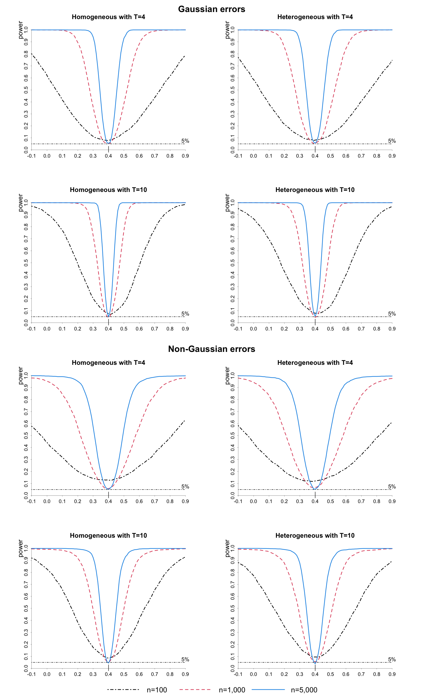
Figure 1: Empirical power functions for FDAC estimator in homogeneous and heterogeneous (a=0.5) panel AR(1) models with Gaussian and non-Gaussian errors, and GARCH effects

Figure 1 in the online supplement displays empirical power functions for the FDAC estimator in the case of homogeneous and heterogeneous panel AR(1) models with both Gaussian and non-Gaussian errors, and GARCH effects. The power functions become steeper as $n$ and $T$ increase. In general, the power of the FDAC estimator is similar under heterogeneous and homogeneous $\phi_{i}$. But with non-Gaussian errors, the power functions become noticeably flatter, and the size distortions become more pronounced for $n=100$.

Table 1: Bias, RMSE, and size of FDAC, FDLS, AH, AAH, AB, and BB estimators of $\phi$ $(\phi_{0}=0.4)$ in a homogeneous panel AR(1) model with Gaussian errors and GARCH effects

			Bias							RMSE							Size ($\times 100$)
$T$	$n$		FDAC	FDLS	AH	AAH	AB	BB		FDAC	FDLS	AH	AAH	AB	BB		FDAC	FDLS	AH	AAH	AB	BB
4	100		-0.002	0.006	0.453	0.096	-0.037	0.014		0.189	0.183	14.925	0.326	0.290	0.171		8.1	9.8	8.0	14.1	12.6	18.4
4	1,000		-0.001	0.001	0.024	0.072	-0.004	0.002		0.062	0.058	0.213	0.222	0.088	0.056		5.4	5.6	4.7	15.9	6.6	6.8
4	5,000		-0.001	-0.001	0.003	0.020	-0.002	0.000		0.029	0.026	0.088	0.121	0.039	0.025		5.5	5.3	4.3	7.1	5.0	4.4
6	100		-0.001	0.004	-0.059	0.028	-0.052	0.014		0.117	0.130	0.215	0.163	0.158	0.107		7.6	8.1	18.8	27.4	21.6	28.8
6	1,000		-0.002	0.000	-0.007	0.000	-0.006	0.002		0.038	0.041	0.067	0.035	0.047	0.032		4.2	5.6	6.5	7.4	7.0	8.2
6	5,000		-0.001	0.000	-0.001	0.001	-0.001	0.001		0.018	0.019	0.031	0.016	0.021	0.014		4.8	4.3	5.3	5.3	4.2	5.0
10	100		0.001	0.003	-0.041	0.008	-0.038	0.004		0.081	0.093	0.099	0.083	0.090	0.068		8.3	8.2	39.8	53.3	45.5	54.5
10	1,000		-0.001	0.000	-0.005	0.001	-0.005	0.001		0.026	0.030	0.030	0.020	0.026	0.019		4.8	6.0	9.5	12.3	10.7	12.4
10	5,000		0.000	0.000	-0.001	0.000	-0.001	0.000		0.012	0.014	0.014	0.009	0.012	0.009		5.5	5.5	6.0	5.9	5.5	5.8

Notes: The DGP is given by $y_{it}=\mu_{i}(1-\phi_{i})+\phi_{i}y_{i,t-1}+u_{it}$ for $i=1,2,...,n$, and $t=-50,-49,...,T$ with $\mu_{i}=\alpha_{i}/(1-\phi_{i})$, where errors, $u_{it}=h_{it}\varepsilon_{it}$, are generated to be Gaussian distributed and cross-sectionally heteroskedastic with GARCH effects: $\varepsilon_{it}\sim IIDN(0,1)$, and $h_{it}^{2}=\sigma_{i}^{2}(1-\psi_{0}-\psi_{1})+\psi_{0}h_{i,t-1}^{2}+\psi_{1}u_{i,t-1}^{2}$ with $\sigma_{i}^{2}\sim IID(0.5+0.5z_{i}^{2})$, $z_{i}\sim IIDN(0,1)$, $\psi_{0}=0.6$, and $\psi_{1}=0.2$. The initial values are given by $y_{i,-51}=0$, $\varepsilon_{i,-51}=0$, and $h_{i,-51}=0$. The AR(1) coefficients are generated to be homogeneous: $\phi_{i}=\phi$ for $i=1,2,...,n$ with $\phi_{0}=0.4$. For each experiment, $(\alpha_{i},\sigma_{i})^{\prime}$ are generated differently across replications. The FDAC estimator is calculated by (6.1), and its asymptotic variance is estimated by the Delta method. “FDLS” denotes the first-difference least square estimator proposed by Han and Phillips (2010). “AH”, “AAH”, “AB”, and “BB” denote the 2-step GMM estimators proposed by Anderson and Hsiao (1981, 1982), Chudik and Pesaran (2021), Arellano and Bond (1991), and Blundell and Bond (1998). The estimation is based on $\{y_{i1},y_{i2},...,y_{iT}\}$ for $i=1,2,...,n$. The nominal size of the tests is set to 5 per cent. The number of replications is $2,000$.

Table 2: Bias, RMSE, and size of FDAC, FDLS, AH, AAH, AB, and BB estimators in a heterogeneous panel AR(1) model with uniformly distributed autoregressive coefficients, $\phi_{i}=\mu_{\phi}+v_{i}$, $\mu_{\phi}=0.4$, and $v_{i}\sim IIDU(-0.3,0.3)$, Gaussian errors, and GARCH effects

			Bias							RMSE							Size ($\times 100$)
$T$	$n$		FDAC	FDLS	AH	AAH	AB	BB		FDAC	FDLS	AH	AAH	AB	BB		FDAC	FDLS	AH	AAH	AB	BB
4	100		-0.001	-0.012	-0.035	0.064	-0.074	0.007		0.192	0.188	9.664	0.304	0.339	0.180		8.6	10.2	9.8	14.8	14.0	19.8
4	1,000		-0.001	-0.021	-0.051	0.021	-0.030	-0.013		0.064	0.064	0.203	0.182	0.102	0.061		5.3	6.6	9.8	16.0	9.0	7.4
4	5,000		0.000	-0.022	-0.068	-0.024	-0.025	-0.017		0.029	0.035	0.108	0.062	0.049	0.032		5.2	12.2	17.8	14.5	10.5	10.5
6	100		0.000	-0.016	-0.101	0.011	-0.084	0.006		0.123	0.135	0.235	0.153	0.184	0.115		7.5	8.8	22.7	23.9	26.0	30.1
6	1,000		-0.002	-0.022	-0.054	-0.010	-0.030	-0.007		0.040	0.048	0.087	0.038	0.061	0.036		4.3	8.3	17.0	8.0	12.3	9.6
6	5,000		0.000	-0.021	-0.048	-0.010	-0.022	-0.006		0.019	0.029	0.057	0.018	0.032	0.017		5.3	19.4	36.4	8.9	17.2	7.8
10	100		0.002	-0.018	-0.063	-0.002	-0.056	0.001		0.086	0.099	0.117	0.088	0.107	0.078		8.3	7.8	45.0	52.1	49.0	58.4
10	1,000		-0.001	-0.022	-0.028	0.001	-0.019	0.003		0.028	0.038	0.044	0.023	0.035	0.022		5.6	11.7	23.0	8.7	17.0	12.3
10	5,000		0.000	-0.022	-0.024	0.003	-0.013	0.006		0.013	0.026	0.029	0.010	0.019	0.011		5.3	34.8	40.1	4.3	19.1	10.7

Notes: The DGP is given by $y_{it}=\mu_{i}(1-\phi_{i})+\phi_{i}y_{i,t-1}+u_{it}$ for $i=1,2,...,n$, and $t=-50,-49,...,T$ with $\mu_{i}=\alpha_{i}/(1-\phi_{i})$ featuring Gaussian distributed errors with GARCH effects. The heterogeneous AR(1) coefficients are generated as case (a): $\phi_{i}=\mu_{\phi}+v_{i}$ with $\mu_{\phi}=0.4$, $v_{i}\sim IIDU(-a,a)$, and $a=0.3$. The FDAC estimator is calculated based on (6.1), and its asymptotic variance is estimated by the Delta method. “FDLS” denotes the first-difference least square estimator proposed by Han and Phillips (2010). “AH”, “AAH”, “AB”, and “BB” denote the 2-step GMM estimators proposed by Anderson and Hsiao (1981, 1982), Chudik and Pesaran (2021), Arellano and Bond (1991), and Blundell and Bond (1998). The estimation is based on $\{y_{i1},y_{i2},...,y_{iT}\}$ for $i=1,2,...,n$. The nominal size of the tests is set to 5 per cent. The number of replications is $2,000$. See also the notes to Table 1.

Table 3: Bias, RMSE, and size of FDAC, FDLS, AH, AAH, AB, and BB estimators in a heterogeneous panel AR(1) model with uniformly distributed autoregressive coefficients, $\phi_{i}=\mu_{\phi}+v_{i}$, $\mu_{\phi}=0.4$, and $v_{i}\sim IIDU(-0.5,0.5)$, Gaussian errors, and GARCH effects

			Bias							RMSE							Size ($\times 100$)
$T$	$n$		FDAC	FDLS	AH	AAH	AB	BB		FDAC	FDLS	AH	AAH	AB	BB		FDAC	FDLS	AH	AAH	AB	BB
4	100		0.000	-0.048	-0.092	0.013	-0.162	0.012		0.201	0.200	3.690	0.287	0.423	0.219		8.2	10.3	14.5	18.4	19.5	26.7
4	1,000		-0.001	-0.061	-0.172	-0.053	-0.112	-0.047		0.067	0.088	0.245	0.135	0.170	0.083		5.2	17.0	28.4	23.0	23.2	15.8
4	5,000		0.000	-0.062	-0.185	-0.072	-0.104	-0.056		0.031	0.068	0.200	0.078	0.118	0.064		5.7	59.4	70.2	62.9	51.2	47.5
6	100		0.001	-0.053	-0.185	-0.017	-0.167	0.011		0.133	0.151	0.286	0.146	0.253	0.144		8.0	10.9	34.7	23.4	39.0	39.8
6	1,000		-0.002	-0.062	-0.143	-0.031	-0.112	-0.029		0.043	0.077	0.160	0.048	0.130	0.049		4.6	29.1	58.9	14.8	50.6	19.4
6	5,000		-0.001	-0.061	-0.138	-0.031	-0.102	-0.027		0.020	0.065	0.142	0.035	0.107	0.032		5.5	86.3	98.9	39.2	94.0	36.8
10	100		0.002	-0.056	-0.121	-0.028	-0.110	0.010		0.095	0.119	0.166	0.101	0.155	0.104		8.5	12.2	60.9	52.3	63.3	66.1
10	1,000		-0.001	-0.062	-0.091	-0.021	-0.079	-0.010		0.031	0.070	0.099	0.036	0.088	0.030		5.3	45.6	75.7	16.3	71.1	17.8
10	5,000		0.000	-0.062	-0.087	-0.019	-0.072	-0.003		0.014	0.064	0.089	0.023	0.074	0.014		5.4	98.4	99.8	29.4	99.0	11.6

Notes: The DGP is given by $y_{it}=\mu_{i}(1-\phi_{i})+\phi_{i}y_{i,t-1}+u_{it}$ for $i=1,2,...,n$, and $t=-50,-49,...,T$ with $\mu_{i}=\alpha_{i}/(1-\phi_{i})$ featuring Gaussian distributed errors with GARCH effects. The heterogeneous AR(1) coefficients are generated as case (a): $\phi_{i}=\mu_{\phi}+v_{i}$ and $v_{i}\sim IIDU(-a,a)$ with $\mu_{\phi}=0.4$ and $a=0.5$. For each experiment, $(\alpha_{i},\phi_{i},\sigma_{i})^{\prime}$ are generated differently across replications. The FDAC estimator is calculated by (6.1), and its asymptotic variance is estimated by the Delta method. “FDLS” denotes the first-difference least square estimator proposed by Han and Phillips (2010). “AH”, “AAH”, “AB”, and “BB” denote the 2-step GMM estimators proposed by Anderson and Hsiao (1981, 1982), Chudik and Pesaran (2021), Arellano and Bond (1991), and Blundell and Bond (1998). The estimation is based on $\{y_{i1},y_{i2},...,y_{iT}\}$ for $i=1,2,...,n$. The nominal size of the tests is set to 5 per cent. The number of replications is $2,000$. See also the notes to Table 1.

7.4 Comparison of FDAC and MSW estimators

This section compares the small-sample performance of the FDAC estimator with the MSW estimator by Mavroeidis et al. (2015). Table 4 reports bias, RMSE, and size of the FDAC and MSW estimators for $E(\phi_{i})$ for $T=4,6,10$, and $n=100,1000$, under heterogeneous $\left(\alpha_{i},\phi_{i}\right)$ with $\mu_{\phi}=0.4$, and Gaussian errors with GARCH effects. The left panel of the table reports the results for $a=0.3$, and the right panel for $a=0.5$. The performance of the FDAC estimator is in line with the ones already discussed and as noted earlier is not affected by the degree of heterogeneity for stationary outcome processes. In contrast, the performance of the MSW estimator seems to depend critically on the degree of heterogeneity. When $a=0.3$, and $T=4$ or $8$, the MSW estimator performs better than the FDAC estimator in terms of bias and RMSE, but exhibits mild size distortions when $n=100$ and $T=6$ or $10$. However, the MSW estimator breaks down if we consider the results for $a=0.5$. For example, the RMSE of the MSW estimator for $T=4$ and $n=1,000$ rises from $0.030$ when $a=0.3$ to $0.246$ when $a=0.5$. The size of the MSW estimator also rises from $10.7$ per cent to $99.7$ per cent as $a$ is increased from $0.3$ to $0.5$, for the same sample sizes.

Table 4: Bias, RMSE, and size of FDAC and MSW estimators in a heterogeneous panel AR(1) model where $\phi_{i}=\mu_{\phi}+v_{i}$ and $v_{i}\sim IIDU(-a,a)$ with $\mu_{\phi}=0.4$, $a\in\{0.3,0.5\}$, Gaussian errors, and GARCH effects

		Medium degree of heterogeneity $a=0.3$									High degree of heterogeneity $a=0.5$
		Bias			RMSE			Size ($\times 100$)			Bias			RMSE			Size ($\times 100$)
$T$	$n$	FDAC	MSW		FDAC	MSW		FDAC	MSW		FDAC	MSW		FDAC	MSW		FDAC	MSW
4	100	-0.005	0.003		0.165	0.084		6.8	6.8		-0.005	0.248		0.168	0.300		7.3	34.4
4	1,000	0.001	0.007		0.050	0.030		3.8	10.7		0.001	0.240		0.052	0.246		4.4	99.7
6	100	0.002	0.012		0.099	0.084		6.0	4.4		0.004	0.260		0.106	0.310		5.8	36.2
6	1,000	0.000	0.023		0.031	0.036		5.1	15.5		0.000	0.261		0.034	0.266		4.9	100.0
10	100	0.000	0.020		0.070	0.089		6.4	4.7		0.001	0.265		0.078	0.315		6.5	37.4
10	1,000	0.001	0.024		0.022	0.038		4.3	15.2		0.001	0.263		0.024	0.269		4.5	100.0

Notes: The DGP is given by $y_{it}=\mu_{i}(1-\phi_{i})+\phi_{i}y_{i,t-1}+u_{it}$ for $i=1,2,...,n$, and $t=-50,-49,...,T$ with $\mu_{i}=\alpha_{i}/(1-\phi_{i})$ featuring Gaussian errors with GARCH effects. The heterogeneous AR(1) coefficients are generated as case (a): $\phi_{i}=\mu_{\phi}+v_{i}$ and $v_{i}\sim IIDU(-a,a)$ with $\mu_{\phi}=0.4$ and $a\in\{0.3,0.5\}$. The FDAC estimator is calculated by (6.1), and its asymptotic variance is estimated by the Delta method. “MSW” denotes the kernel-weighting likelihood estimator proposed by Mavroeidis et al. (2015) and calculated assuming that $(\alpha_{i},\phi_{i})|y_{i1}\sim IIDN(\boldsymbol{\mu},\boldsymbol{V})$ with initial values given by $\boldsymbol{\mu}=(5,0.5)$, $\sigma_{\alpha}=2$, $\sigma_{\phi}=0.4$, $corr(\alpha_{i},\phi_{i})=0.5$ and $\sigma_{u}=0.5$. The nominal size of the tests is set to 5 per cent. Due to the extensive computations required for the implementation of the MSW estimator, the number of replications is $1,000$.

7.5 Non-stationary initialization

One of the key assumptions behind the FDAC estimator is the stationarity of $\{y_{it}\}$. This assumption requires that the initial values $\left\{y_{i0}\right\}$ are drawn from the steady state distribution of the underlying processes, which is given by

$$y_{i0}=\mu_{i}+v_{i},\text{ and }v_{i}\thicksim IID\left(0,\sigma_{i}^{2}/(1-\phi_{i}^{2})\right),$$ (7.1)

where $\mu_{i}=\alpha_{i}/(1-\phi_{i})$. As shown in Section S.3 of the online supplement, the moment conditions (4.1) and (4.2) can also be derived under the above initial distribution, but need not hold if the distribution of $y_{i0}$ departs from the steady state distribution. The same is also true for some of the HomoGMM estimators. It is, therefore, of interest to investigate the sensitivity of the FDAC and HomoGMM estimators to departures from the steady state distribution in (7.1). Here we model this departure by assuming that $\left\{y_{it}\right\}$ starts from $M$ periods before the first observation, $y_{i1}$, used in the estimation process. Assuming that all $n$ AR(1) processes are generated from $y_{i,-M}$ $\left(\left|y_{i,-M}\right|<C\text{, }\left|\phi_{i}\right|<1\right)$ we have

$$y_{i0}=\mu_{i}(1-\phi_{i}^{M})+\phi_{i}^{M}y_{i,-M}+\sum_{s=0}^{M-1}\phi_{i}^{s}u_{i,-s}.$$ (7.2)

It is clear that as $M\rightarrow\infty$, the distribution of $y_{i0}$ converges to the steady state distribution given by (7.1). This suggests that departures from the steady state distribution can be conveniently represented by using relatively small values of $M$. To investigate the effects of departures from the steady state distribution, we generate the initial values as $y_{i0}\sim IIDN\left[\mu_{i}(1-\phi_{i}^{M}),\sigma_{i}^{2}(1-\phi_{i}^{2M})/(1-\phi_{i}^{2})\right]$, which converges to the stationary distribution as $M\rightarrow\infty$. We consider both homogeneous and heterogeneous cases and set $\phi_{i}=0.4+v_{i}$, where $v_{i}\thicksim IIDU(-a,a)$, with $a\in\left\{0,0.3,0.5\right\}$. In the case of non-stationary initial values, the distribution of the FDAC estimator, as well as a number of GMM estimators, depends on the the ratio $\kappa^{2}=$ $Var(\alpha_{i})/Var(u_{it})$, which in the case of our MC design reduces to $\kappa^{2}=Var(v_{i})+Var(\eta_{i})=a^{2}/3+Var(\eta_{i})$. It is clear that $\kappa^{2}$ is dominated by $Var(\eta_{i})$ and to highlight the dependence of $FDAC$ and other estimators on $M$ and $\kappa^{2}$ we consider the following combinations $M=\{1,2,15\}$ and $Var(\eta_{i})=\{1,3,5\}$. The MC results for these combinations are summarized in the online supplement. The results for the homogeneous case ($\alpha=0),$ are given in Tables S.8 to S.10, and for the heterogeneous cases are summarized in Tables S.11 to S.13 for $a=0.3,$ and in Tables S.14–S.16 for $a=0.5$.

In the homogeneous case ($a=0$), when $M=1$, the FDAC, FDLS, and BB estimators all show sizeable bias and size distortions that do not vanish as $n$ increases. The magnitudes of bias, RMSE, and size distortions are larger for higher $\kappa^{2}$. This is particularly noticeable for the BB estimator, a result already highlighted by Chudik and Pesaran (2021). Also, as to be expected, under homogeneity, the AH, AAH, and AB estimators are robust to non-stationary initialization and have similar performance across different values of $M$ and $\kappa^{2}$.

In the case of heterogeneous panels, the FDAC estimator is adversely affected when $M=1$ or $2$, and displays bias and size distortions, particularly when there is a high degree of heterogeneity (namely $a=0.5$), and the magnitude of the bias and size distortion rises with $\kappa^{2}$. But, as to be expected, the bias and size distortion of FDAC disappear as $M$ is increased. Note that the results for $M=15$ with $Var(\eta_{i})=1$ are comparable to the results in Tables 2 and 3 where $\{y_{it}\}$ are generated starting with $y_{i,-51}=0$. For the HomoGMM estimators, the magnitude of neglected heterogeneity bias is much larger, and the size distortions are much more serious and in general, increase with $\kappa^{2}$ when $M=1$ or $2$, as compared to $M=15$ (which approximately corresponds to the stationary case).

In brief, when $M$ is sufficiently large, the performance of the FDAC is not affected by the relative size of the individual fixed effects, $\kappa^{2}$, under both slope homogeneity and heterogeneity. Nonetheless, it is clearly a challenge to simultaneously deal with heterogeneity of $\phi_{i}$ and the non-stationarity that arises when $y_{i0}$ are not drawn from the steady state distribution of $\{y_{it}\}$.

7.6 Simulation results for the categorical distribution parameters

Section 5 has already shown that assuming $\phi_{i}$ follow a categorical distribution with a finite number of categories, the parameters of the underlying categorical distribution can be identified from the moments of $\phi_{i}$ under stationarity. Here we investigate the finite sample performance of estimating the parameters in the simple case of two categories, namely $\phi_{L},\phi_{H}$ and $\pi$. Since the procedure for estimating these parameters is based on the first three moments, then we need $T\geq 6$. See equation (6.3). Precise estimation of $\phi_{L}$ and $\phi_{H}$ also require quite large samples. Accordingly, we consider the following sample sizes: $T=6,8,10,$ and $n=2000,5000,10000,50000$.

Table 5 reports the bias and RMSE of the plug-in estimators given by (5.1) and (5.5), using the FDAC estimators of the moments of $\phi_{i}$. Compared with the simulation results for $E(\phi_{i})$ and $Var(\phi_{i}$), the FDAC estimators of $\phi_{L},\phi_{H},$ and $\pi$ have much larger RMSEs. Also, the magnitude of bias and RMSE of $\phi_{L}$ and $\phi_{H}$ are much larger than those of $\pi$, particularly when $T=6$. Since the moment conditions of categorical distribution are linear in $\pi$ but nonlinear in $\phi_{L}$ and $\phi_{H}$, the nonlinearity plays a crucial role here. Given equation (5.5), the solutions of $\phi_{L}$ and $\phi_{H}$ are ratios of functions of moments. The denominator is given by the variance of $\phi_{i}$, which could be close to zero in finite samples, and thus, minor estimation errors in the denominator could have large adverse effects on the precision with which $\phi_{L}$ and $\phi_{H}$ can be estimated.

RMSEs of the FDAC estimators of $\phi_{L},\phi_{H},$ and $\pi$ decline rapidly with $n$ for a given $T$. For example, RMSE of $\phi_{H}$ declines from $0.217$ for $T=8$ and $n=2,000,$ to $0.068$ for $T=8$ and $n=10,000$. Similar results are obtained by Gao and Pesaran (2023) in the case of pure cross-sectional regressions where it is also shown that relatively large values of $n$ are required for precise estimation of the parameters of the categorical distribution.

Table 5: Bias and RMSE of FDAC estimator of categorical distribution parameters $(\phi_{L},\phi_{H},\pi)^{\prime}$ with Gaussian errors and GARCH effects

			$\phi_{i}=0.4+v_{i}$, $v_{i}\sim IIDU(-0.3,0.3)$									$\phi_{i}=0.4+v_{i}$, $v_{i}\sim IIDU(-0.5,0.5)$									Categorical distributed $\phi_{i}$
			$\phi_{L}=0.11$			$\phi_{H}=0.69$			$\pi=0.5$			$\phi_{L}=0.11$			$\phi_{H}=0.69$			$\pi=0.5$			$\phi_{L}=0.2$			$\phi_{H}=0.8$			$\pi=0.3$
$T$	$n$		Bias	RMSE		Bias	RMSE		Bias	RMSE		Bias	RMSE		Bias	RMSE		Bias	RMSE		Bias	RMSE		Bias	RMSE		Bias	RMSE
6	2,000		-0.108	0.663		0.225	2.782		0.019	0.309		0.434	15.414		0.710	17.534		0.021	0.442		-0.373	5.974		0.321	2.476		0.103	0.336
6	5,000		-0.036	0.193		0.073	0.264		0.016	0.239		0.034	9.148		1.786	58.043		0.020	0.405		-0.042	0.271		0.084	0.678		0.068	0.256
6	10,000		-0.017	0.129		0.035	0.145		0.012	0.188		-0.216	1.438		0.405	2.856		0.015	0.375		-0.018	0.183		0.031	0.119		0.043	0.191
6	50,000		-0.006	0.058		0.006	0.054		0.001	0.094		-0.047	0.163		0.061	0.211		0.003	0.277		-0.004	0.084		0.005	0.035		0.010	0.084
8	2,000		-0.041	0.216		0.089	0.784		0.020	0.252		-0.460	7.728		3.726	166.514		0.023	0.412		-0.067	0.678		0.130	1.028		0.079	0.272
8	5,000		-0.012	0.120		0.033	0.134		0.015	0.179		-0.099	1.337		0.296	4.758		0.023	0.367		-0.010	0.172		0.029	0.104		0.045	0.185
8	10,000		-0.005	0.085		0.017	0.084		0.011	0.134		-0.077	0.267		0.188	0.864		0.027	0.329		-0.007	0.121		0.012	0.061		0.022	0.130
8	50,000		-0.002	0.039		0.003	0.035		0.002	0.063		-0.018	0.100		0.030	0.115		0.011	0.215		0.000	0.055		0.002	0.021		0.006	0.054
10	2,000		-0.023	0.208		0.054	0.235		0.016	0.214		-0.280	5.066		0.211	9.146		0.021	0.396		-0.021	0.225		0.053	0.218		0.065	0.233
10	5,000		-0.010	0.098		0.019	0.098		0.009	0.150		-0.104	0.318		0.374	5.242		0.017	0.344		-0.006	0.138		0.017	0.068		0.031	0.147
10	10,000		-0.004	0.068		0.010	0.064		0.006	0.110		-0.052	0.193		0.100	0.314		0.019	0.299		-0.005	0.099		0.008	0.044		0.015	0.103
10	50,000		-0.001	0.031		0.002	0.027		0.002	0.050		-0.011	0.077		0.020	0.082		0.012	0.182		-0.001	0.045		0.002	0.017		0.003	0.044

Notes: The DGP is given by $y_{it}=\mu_{i}(1-\phi_{i})+\phi_{i}y_{i,t-1}+u_{it}$ for $i=1,2,...,n$, and $t=-50,-49,...,T$ with $\mu_{i}=\alpha_{i}/(1-\phi_{i})$ featuring Gaussian errors with GARCH effects. The heterogeneous AR(1) coefficients are generated by case (a): uniform distribution $\phi_{i}=\mu_{\phi}+v_{i}$ and $v_{i}\sim IIDU(-a,a)$ with $\mu_{\phi}=0.4$ and $a\in\{0.3,0.5\}$, and case (b): categorical distribution $\text{Pr}(\phi_{i}=\phi_{L})=\pi$ and $\text{Pr}(\phi_{i}=\phi_{H})=1-\pi$ with $\pi=0.3$, $\phi_{L}=0.2$, and $\phi_{H}=0.8$ such that $E(\phi_{i})=0.62$. The FDAC estimator is calculated by (5.1) and (5.5). The number of replications is 2,000.

8 Empirical application: heterogeneity in earnings dynamics

8.1 Literature review of estimation of earnings dynamics

Estimating earnings equations is crucial for answering some of the most important economic questions. Variance of earnings has been modeled and decomposed to measure income uncertainties in Lillard and Weiss (1979), MaCurdy (1982), Carroll and Samwick (1997), Meghir and Pistaferri (2004), Altonji et al. (2013) and to quantify earnings mobility in Lillard and Willis (1978) and Geweke and Keane (2000). The covariance structures between earnings and other households’ characteristics, for example, work hours, consumptions, and savings have been studied by Abowd and Card (1989) Hubbard et al. (1995), Guvenen (2007), and Alan et al. (2018).

Among these studies, a homogeneous AR or ARMA process is often used as a component when modeling innovations in earnings processes. Based on the Restricted Income Profiles model that assumes homogenous linear trends proposed in MaCurdy (1982), MaCurdy (1982) and Hubbard et al. (1995), obtained close to unit root estimates for the AR(1) coefficient, ranging from 0.946 to 0.998. Following this literature, a unit root assumption was imposed in Carroll and Samwick (1997) and Meghir and Pistaferri (2004). On the other hand, using the Heterogeneous Income Profiles, by assuming unit-specific linear trends, Lillard and Weiss (1979) obtained estimates of the AR(1) coefficient (assumed to be homogeneous) ranging from 0.153 to 0.860 for a sample with PhD degrees. Guvenen (2009) using PSID data obtained estimates ranging from 0.809 to 0.899.

There are also a number of studies that allow for heterogeneity in the AR(1) coefficients. Prominent examples are Browning et al. (2010), Alan et al. (2018), Browning et al. (2010), and Gu and Koenker (2017). These studies are typically based on panels with a moderate time dimension and make parametric assumptions regarding the distribution of the AR(1) coefficients; often using a Bayesian framework. The application of the FDAC estimator to earnings equation allows for heterogeneity in the AR(1) coefficients without making any strong parametric assumptions, even when $T$ is as small as $5$. Also because of first-differencing prior to estimation, the FDAC estimator is robust to unobserved individual-specific characteristics and is not subject to misspecification bias that could arise when log real wages are filtered for individual-specific characteristics before investigating the dynamics of the earnings process.

8.2 A heterogeneous panel AR(1) model of earnings dynamics with linear trends

We consider estimating the earnings equation with fixed effects, heterogeneous autoregressive coefficients, without imposing any restrictions on the joint distributions of $\alpha_{i}$, $\phi_{i}$, and $y_{i0}$. However, to accommodate growth in real earnings we extend our baseline model in (2.1) to allow for linear trends:

$$y_{it}=\alpha_{i}+g_{i}(1-\phi_{i})t+\phi_{i}y_{i,t-1}+u_{it},$$ (8.1)

where $y_{it}=log(earnings_{it}/p_{t}),$ $earnings_{it}$ is the reported earnings of individual $i$ in year $t$, $p_{t}$ is a general price, and $g_{i}$ denotes the growth rate of real earnings for individual $i$. The above equation can be written equivalently as

$$\tilde{y}_{it}(g_{i})=b_{i}+\phi_{i}\tilde{y}_{i,t-1}(g_{i})+u_{it},$$

where $\tilde{y}_{it}(g_{i})=y_{it}-g_{i}t$, and $b_{i}=\alpha_{i}-g_{i}\phi_{i}$. The steady state distribution of $y_{it}$ can now be derived using

$$y_{it}=b_{i}+g_{i}t+\sum_{s=0}^{\infty}\phi_{i}^{s}u_{i,t-s}.$$ (8.2)

When $T$ is sufficiently large individual-specific growth rates, $g_{i}$, can be estimated $\sqrt{T}$-consistently by running individual least squares regressions of $y_{it}$ on an intercept and a linear trend, and then using the residuals from these regressions to estimate the moments of $\phi_{i}$. This approach requires $n$ and $T$ to be both large. In the case of the present empirical application where $T$ is short ($5$ or $10)$, we provide estimates of the moments of $\phi_{i}$ assuming that $g_{i}=g$ for individuals within a given group, but allow $g$ to differ across groups, classified by the educational attainment levels. $\sqrt{n}$-consistent estimators of $g$ can be obtained either from the pooled regression of $y_{it}$ on fixed effects and a common linear trend, namely

$$\hat{g}_{FE}=\frac{\sum_{t=1}^{T}(\bar{y}_{\circ t}-\bar{y}_{\circ\circ})t}{\sum_{t=1}^{T}\left(t-\frac{(T+1)}{2}\right)^{2}},$$ (8.3)

with $\bar{y}_{\circ t}=n^{-1}\sum_{i=1}^{n}y_{it}$ and $\bar{y}_{\circ\circ}=T^{-1}n^{-1}\sum_{i=1}^{n}\sum_{t=1}^{T}y_{it}$, or after first-differencing of (8.2) (with $g_{i}=g)$ by

$$\hat{g}_{FD}=\frac{\sum_{t=2}^{T}\sum_{i=1}^{n}\Delta y_{it}}{n(T-1)}.$$ (8.4)

For small $T$ there is little to choose between these two estimators, and they are identical when $T=2$. Given either of the above estimators, generically denoted by $\hat{g}$, $\tilde{y}_{it}(\hat{g})=y_{it}-\hat{g}t$ can now be used to estimate the moments of $\phi_{i}$ using the FDAC or MSW procedures.

In addition to the FDAC estimates, we also present estimates based on four estimation methods assuming homogeneous slope coefficients, namely AAH, AB, and BB estimators proposed by Chudik and Pesaran (2021), Arellano and Bond (1991), and Blundell and Bond (1998), and the MSW estimator of Mavroeidis et al. (2015). Following Meghir and Pistaferri (2004), individuals in each time series sample are divided into three education categories, where “HSD” refers to high school dropouts with less than 12 years of education, “HSG” refers to high school graduates with at least 12 but less than 16 years of education, and “CLG” refers to college graduates with at least 16 years of education. To allow for possible time variations in the estimates of mean earnings persistence we provide estimates for $five$ and $ten$ yearly non-overlapping sub-periods. The five yearly samples are 1976–1980, 1981–1985, 1986–1990, and 1991–1995. The ten yearly samples are 1976–1985, 1981–1990 and 1991–1995. For each sub-period, we provide estimates for all categories combined, as well as separate estimates for the three educational sub-categories. To save space, the results for the last five and ten yearly samples are given in the paper. The estimates for the earlier sub-periods are provided in the online supplement.

Table 6 gives the estimates of mean earnings persistence, $E(\phi_{i}),$ and the common linear trend coefficient, $g$, for the sub-periods 1991–1995 ($T=5$) and 1986–1995 ($T=10$). The estimates of $g$ is on average around $2$ per cent per annum with some modest variations across the sub-samples and educational categories. The HomoGMM estimates (AAH, AB and BB) differ a great deal, both over sub-periods and across educational categories. The AAH estimates are all around 0.50 and show little variations across the two sub-period and the educational categories. The AB estimates tend to be quite low and are not statistically significant for two of the educational categories in the shorter sub-period $(T=5)$. In contrast, the BB estimates are much larger and in many instances are close to unity. For example, for the sub-period 1986-1995 $(T=10)$, the BB estimates of earnings persistence for the three educational categories HSD, HSG and CLG are 0.923 (0.003), 0.914 (0.003) and 0.992 (0.004), respectively, with standard errors in brackets.

We also find sizeable differences in the estimates of mean earnings persistence when we consider the FDAC and MSW estimators. The MSW estimates are all around 0.45 and do not vary with the level of educational attainment. In contrast, the FDAC estimates are somewhat larger (lie in the range of 0.570-0.734) and rise with the level of educational attainment. This pattern can be seen in both sub-periods. For example, for the longer sub-period (1986-1995), the mean persistence for HSD, HSG and CLG categories are estimated to be 0.580 (0.071), 0.611 (0.028) and 0.735 (0.040), respectively. Similar results are obtained for the other sub-periods. See Tables S.29 and S.30 of the online supplement. It is interesting that the higher earnings persistence of the college graduate category is a prominent feature of the FDAC estimates for all sub-periods. This result is also in line with a number of theoretical arguments advanced in the literature in terms of the higher mobility of college graduates and their relative job stability. For example, see Carroll and Samwick (1997) and Carneiro et al. (2023).

Although we have not developed a formal statistical test of the heterogeneity $\phi_{i}$, the estimates of $Var(\phi_{i})$ provide a good indication of the degree of within-group heterogeneity. Estimates of $Var(\phi_{i})$ based on MSW and FDAC procedures for the various sub-periods are given in Tables S.31–S.33 of the online supplement. The FDAC estimates are much larger than the MSW estimates. For example, for the sub-period 1991–1995 the MSW estimates of $Var(\phi_{i})$ are all around 0.011 with standard errors in the range of 0.004–009, whilst the FDAC estimates of $Var(\phi_{i})$ for the same sub-period are 0.241(0.100), 0.081(0.054) and 0.091(0.09) for the three educational categories of HSD, HSG and CLG, respectively. The degree of within-group heterogeneity also seems to vary over time. For example, for the longer sub-period (1986-1995), the FDAC estimates of $Var(\phi_{i})$ are generally larger with lower standard errors for all educational categories.

Table 6: Estimates of mean persistence ($\mu_{\phi}=E(\phi_{i})$) of log real earnings in a panel AR(1) model with a common linear trend using PSID data over the sub-periods 1991–1995 and 1986–1995

	1991–1995, $T=5$						1986–1995, $T=10$
	All		Category by education				All		Category by education
	categories		HSD	HSG	CLG		categories		HSD	HSG	CLG
Homogeneous slopes
AAH	0.526		0.490	0.547	0.447		0.546		0.569	0.535	0.522
	(0.046)		(0.072)	(0.061)	(0.072)		(0.028)		(0.024)	(0.033)	(0.038)
AB	0.278		0.105	0.320	-0.013		0.311		0.310	0.335	0.232
	(0.081)		(0.147)	(0.097)	(0.133)		(0.039)		(0.045)	(0.044)	(0.070)
BB	0.488		0.872	0.602	0.964		0.880		0.923	0.914	0.992
	(0.059)		(0.031)	(0.042)	(0.074)		(0.004)		(0.003)	(0.003)	(0.004)
Heterogeneous slopes
FDAC	0.586		0.582	0.567	0.635		0.636		0.580	0.611	0.734
	(0.042)		(0.132)	(0.056)	(0.065)		(0.023)		(0.071)	(0.028)	(0.040)
MSW	0.437		0.431	0.436	0.452		0.458		0.459	0.452	0.460
	(0.040)		(0.044)	(0.043)	(0.045)		(0.054)		(0.038)	(0.046)	(0.063)
Common linear trend	0.023		0.008	0.027	0.020		0.019		0.024	0.020	0.013
$n$	1,366		127	832	407		1,139		109	689	341

Notes: The estimates are based on $y_{it}=\alpha_{i}+g(1-\phi_{i})t+\phi_{i}y_{i,t-1}+u_{it}$, where $y_{it}=log(earnings_{it}/p_{t})$ using the PSID data over the sub-periods 1991–1995 and 1986–1995. “HSD” refers to high school dropouts with less than 12 years of education, “HSG” refers to high school graduates with at least 12 but less than 16 years of education, and “CLG” refers to college graduates with at least 16 years of education. $\hat{g}_{FD}$ is computed by (8.4). The estimation for $\mu_{\phi}$ is based on $\tilde{y}_{it}=y_{it}-\hat{g}_{FD}t$ for $t=1,2,...,T$. “AAH”, “AB”, and “BB” denote the 2-step GMM estimators proposed by Chudik and Pesaran (2021), Arellano and Bond (1991), and Blundell and Bond (1998). The FDAC estimator is calculated by (6.1), and its asymptotic variance is estimated by the Delta method. “MSW” denotes the kernel-weighted estimator in Mavroeidis et al. (2015).

9 Conclusion

This paper considers the estimation of heterogeneous panel AR(1) data models with short (and fixed) $T$, as $n\rightarrow\infty$. It allows for fixed effects and proposes estimating the moments of the AR(1) coefficients, $E(\phi_{i}^{s})$, for $s=1,2,...,S$, using the autocorelation function of first differences. We also show how estimates of $E(\phi_{i}^{s})$, can be used to identify the underlying distribution of $\phi_{i}$, assuming they follow categorical distributions. It is also shown that the standard GMM estimators proposed in the literature for short $T$ panels are inconsistent in the presence of slope heterogeneity. Analytical expressions for this bias are derived and shown to be very close to estimates obtained from stochastic simulations.

The small sample properties of the proposed estimators are investigated using Monte Carlo experiments. Under stationarity of the outcome processes, it is shown that the FDAC estimator which is based on the autocorrelations of first-differences (set out in sub-section 6.1) performs much better than the HetroGMM estimator based on autocovariances of the first differences (set out in sub-section 6.2). Focussing on the FDAC estimator, we find that the FDAC estimator performs well even under homogeneous AR(1) coefficients. The magnitudes of bias and RMSE of the FDAC estimators are comparable to the HomoGMM estimators, and the size of the tests based on the FDAC estimator is mostly around the 5 per cent nominal level. The simulation results also confirm the presence of neglected heterogeneity bias of the HomoGMM estimators under slope heterogeneity, which can result in substantial size distortions. The FDAC estimator is shown to be reliable for stationary heterogeneous panel AR(1) models. The simulation results also show that the FDAC estimator is robust to different distributions of autoregressive coefficients and error processes. However, when the initialization of the outcome process deviates from the steady state distribution, the FDAC estimator could suffer from bias and size distortions. We also find that for the estimation of the parameters of the categorical distribution large sample sizes are required.

The utility of the FDAC estimator is illustrated by applying it to the 1976–1995 PSID data using heterogeneous AR(1) panels in log real earnings with a common linear trend. We provide estimates of $E(\phi_{i})$ and $Var(\phi_{i})$ over a number of $5$ and $10$ yearly sub-periods, with 3 educational groupings. The estimates of $E(\phi_{i})$ differ systematically across the education groups, with the mean persistence of real earnings rising with the level of educational attainments (high school dropouts, high school graduates, and college graduates). The estimates of $Var(\phi_{i})$ differ across periods and levels of educational attainment, but do not display any particular patterns.

It is, however, important to acknowledge that the scope of the present paper is limited, with a number of remaining challenges: (a) allowing for individual-specific time-varying covariates, such as heterogeneous time trends, and (b) simultaneously dealing with heterogeneity and non-stationary initialization. It is not clear that such extensions will be possible without relaxing the assumption that $T$ is short and fixed, as $n\rightarrow\infty$. But these are clearly important topics for future research.

S.1 Introduction

This online supplement is organized as follows: Section S.2 derives expressions for the analytical bias of the AB and BB estimators under heterogeneity of $\phi_{i}$ when $T=4$. Section S.3 derives the autocovariances of first differences assuming the initial values are random draws from the steady state distribution of $\{y_{it}\}$. Section S.4 provides additional Monte Carlo evidence. Section S.5 describes the sample (1976–1995) of the Panel Study of Income Dynamics (PSID) data used in the empirical application, and provides estimation results for a number of sub-periods in addition to the ones reported in the main paper.

S.2 Neglected heterogeneity bias in AB and BB estimators

The AB estimator proposed by Arellano and Bond (1991) is based on the following moment conditions:

$$E(y_{is}\Delta u_{it})=0\text{, for }i=1,2,...,n,s=1,2,...,t-2\text{, and }t=3,4,...,T,$$ (S.1)

which can also be written as $E[y_{is}(\Delta y_{it}-\phi_{i}\Delta y_{i,t-1})]=0,$ with $(T-1)(T-2)/2$ moment conditions in total. When $T=4$, the AB moment conditions, neglecting the heterogeneity, are given by $E[y_{i1}(\Delta y_{i3}-\phi\Delta y_{i2})]=0$, $E[y_{i1}(\Delta y_{i4}-\phi\Delta y_{i3})]=0$, and $E[y_{i2}(\Delta y_{i4}-\phi\Delta y_{i3})]=0$. With a fixed weight matrix $\boldsymbol{W}_{AB}$, the AB estimator can be written as

$$\hat{\phi}_{AB}=\left(\boldsymbol{\bar{z}}_{na}^{\prime}\boldsymbol{W}_{AB}\boldsymbol{\bar{z}}_{na}\right)^{-1}\left(\boldsymbol{\bar{z}}_{na}^{\prime}\boldsymbol{W}_{AB}\boldsymbol{\bar{z}}_{nb}\right),$$ (S.2)

where $\boldsymbol{\bar{z}}_{na}=n^{-1}\left(\sum_{i=1}^{n}y_{i1}\Delta y_{i2},\sum_{i=1}^{n}y_{i1}\Delta y_{i3},\sum_{i=1}^{n}y_{i2}\Delta y_{i3}\right)^{\prime},$ and

$\boldsymbol{\bar{z}}_{nb}=n^{-1}\left(\sum_{i=1}^{n}y_{i1}\Delta y_{i3},\sum_{i=1}^{n}y_{i1}\Delta y_{i4},\sum_{i=1}^{n}y_{i2}\Delta y_{i4}\right)^{\prime}.$ Under Assumptions 2 and 3,

$$y_{it}=(1-\phi_{i})^{-1}\alpha_{i}+\sum_{\ell=0}^{\infty}\phi_{i}^{\ell}u_{i,t-\ell},$$ (S.3)

and assuming that $\alpha_{i}$ is distributed independently of $\{u_{it}\}$ (as assumed under AB) then using (3.2) and (S.3) we have

$$E\left(y_{i,t-h}\Delta y_{it}|\alpha_{i},\phi_{i},\sigma_{i}^{2}\right)$$

$$= E\left[\left.\left(\alpha_{i}\sum_{\ell=0}^{\infty}\phi_{i}^{\ell}+\sum_{\ell=0}^{\infty}\phi_{i}^{\ell}u_{i,t-\ell}\right)\left(u_{it}-(1-\phi_{i})\sum_{\ell=1}^{\infty}\phi_{i}^{\ell-1}u_{i,t-\ell}\right)\right|\alpha_{i},\phi_{i},\sigma_{i}^{2}\right]$$

$$= -E\left[\left.(1-\phi_{i})\left(\sum_{\ell=0}^{\infty}\phi_{i}^{h-1+2\ell}u_{i,t-h-\ell}^{2}\right)\right|\phi_{i},\sigma_{i}^{2}\right]=-\frac{\sigma_{i}^{2}(1-\phi_{i})\phi_{i}^{h-1}}{1-\phi_{i}^{2}},$$

Hence

$$E\left(y_{i,t-h}\Delta y_{it}\right)=-E\left(\frac{\sigma_{i}^{2}\phi_{i}^{h-1}}{1+\phi_{i}}\right)\text{, for }h=1,2,....$$ (S.4)

Given (S.4), we have

$$\boldsymbol{z}_{a}=\underset{n\rightarrow\infty}{plim}\boldsymbol{\bar{z}}_{na} =-\left(E\left(\frac{\sigma_{i}^{2}}{1+\phi_{i}}\right),E\left(\frac{\sigma_{i}^{2}\phi_{i}}{1+\phi_{i}}\right),E\left(\frac{\sigma_{i}^{2}}{1+\phi_{i}}\right)\right)^{\prime},$$

$$\text{and}\quad\boldsymbol{z}_{b}=\underset{n\rightarrow\infty}{plim}\boldsymbol{\bar{z}}_{nb} =-\left(E\left(\frac{\sigma_{i}^{2}\phi_{i}}{1+\phi_{i}}\right),E\left(\frac{\sigma_{i}^{2}\phi_{i}^{2}}{1+\phi_{i}}\right),E\left(\frac{\sigma_{i}^{2}\phi_{i}}{1+\phi_{i}}\right)\right)^{\prime}.$$

Thus, when $\phi_{i}=\mu_{\phi}+v_{i}$ distributed independently of $\sigma_{i}^{2}$ with $v_{i}$ $\thicksim IIDU(-a,a),$ for $a>0$,

$$\underset{n\rightarrow\infty}{plim}\left(\hat{\phi}_{AB}-E(\phi_{i})\right)=\left(\boldsymbol{z}_{a}^{\prime}\boldsymbol{W}_{AB}\boldsymbol{z}_{na}\right)^{-1}\left(\boldsymbol{z}_{a}^{\prime}\boldsymbol{W}_{AB}\boldsymbol{z}_{b}\right)-\mu_{\phi},$$ (S.5)

where $\boldsymbol{z}_{a}=-\sigma^{2}(c_{\phi},1-c_{\phi},c_{\phi})^{\prime}$ and $\boldsymbol{z}_{a}=-\sigma^{2}(1-c_{\phi},\mu_{\phi}-1+c_{\phi},1-c_{\phi})^{\prime}$ with $\sigma^{2}=E(\sigma_{i}^{2})$ and $c_{\phi}=E\left(\frac{1}{1+\phi_{i}}\right)=\frac{1}{2a}\ln\left(\frac{1+\mu_{\phi}+a}{1+\mu_{\phi}-a}\right)$.

In addition to (S.1), consider the following moment condition also used in the system GMM estimator proposed by Blundell and Bond (1998) given by

$$E[\Delta y_{i,t-1}(\alpha_{i}+u_{it})]=0\text{, for }i=1,2,...,n,\text{, and }t=3,4,...,T,$$ (S.6)

which can also be written as $E[\Delta y_{i,t-1}(y_{it}-\phi y_{i,t-1})]=0.$ For $T=4$, with a fixed weight matrix $\boldsymbol{W}_{BB}$, the BB estimator combining moment conditions in (S.1) and (S.6) is given by

$$\hat{\phi}_{BB}=\left(\boldsymbol{\bar{z}}_{nc}^{\prime}\boldsymbol{W}_{BB}\boldsymbol{\bar{z}}_{nc}\right)^{-1}\left(\boldsymbol{\bar{z}}_{nc}^{\prime}\boldsymbol{W}_{BB}\boldsymbol{\bar{z}}_{nd}\right),$$ (S.7)

where

$$\boldsymbol{\bar{z}}_{nc} =n^{-1}\left(\sum_{i=1}^{n}y_{i1}\Delta y_{i2},\,\sum_{i=1}^{n}y_{i1}\Delta y_{i3},\sum_{i=1}^{n}y_{i2}\Delta y_{i3},\sum_{i=1}^{n}y_{i2}\Delta y_{i2},\sum_{i=1}^{n}y_{i3}\Delta y_{i3}\right)^{\prime},$$

$$\text{and}\quad\boldsymbol{\bar{z}}_{nd} =n^{-1}\left(\sum_{i=1}^{n}y_{i1}\Delta y_{i3},\sum_{i=1}^{n}y_{i1}\Delta y_{i4},\sum_{i=1}^{n}y_{i2}\Delta y_{i4},\sum_{i=1}^{n}y_{i3}\Delta y_{i2},\sum_{i=1}^{n}y_{i4}\Delta y_{i3}\right)^{\prime}.$$

Using (3.2) and (S.3), similarly, we can derive the following equations

$$E\left(y_{it}\Delta y_{i,t-h}\right)=E\left(\frac{\sigma_{i}^{2}\phi_{i}^{h}}{1+\phi_{i}}\right)\text{, for }h=0,1,2,...,$$ (S.8)

and it follows that

$$\boldsymbol{z}_{c} =\underset{n\rightarrow\infty}{plim}\boldsymbol{\bar{z}}_{nc}=\left(-E\left(\frac{\sigma_{i}^{2}}{1+\phi_{i}}\right),-E\left(\frac{\sigma_{i}^{2}\phi_{i}}{1+\phi_{i}}\right),-E\left(\frac{\sigma_{i}^{2}}{1+\phi_{i}}\right),E\left(\frac{\sigma_{i}^{2}}{1+\phi_{i}}\right),E\left(\frac{\sigma_{i}^{2}}{1+\phi_{i}}\right)\right)^{\prime},$$

$$\boldsymbol{z}_{d} =\underset{n\rightarrow\infty}{plim}\boldsymbol{\bar{z}}_{nd}$$

$$=\left(-E\left(\frac{\sigma_{i}^{2}\phi_{i}}{1+\phi_{i}}\right),-E\left(\frac{\sigma_{i}^{2}\phi_{i}^{2}}{1+\phi_{i}}\right),-E\left(\frac{\sigma_{i}^{2}\phi_{i}}{1+\phi_{i}}\right),E\left(\sigma_{i}^{2}-\frac{\sigma_{i}^{2}}{1+\phi_{i}}\right),E\left(\sigma_{i}^{2}-\frac{\sigma_{i}^{2}}{1+\phi_{i}}\right)\right)^{\prime}.$$

Thus, when $\phi_{i}$ and $\sigma_{i}^{2}$ are distributed independently and $\phi_{i}=\mu_{\phi}+v_{i}$ where $v_{i}$ $\thicksim IIDU(-a,a),$ for $a>0$, we have

$$plim_{n\rightarrow\infty}\left[\hat{\phi}_{BB}-E(\phi_{i})\right]=\left(\boldsymbol{z}_{c}^{\prime}\boldsymbol{W}_{BB}\boldsymbol{z}_{c}\right)^{-1}\left(\boldsymbol{z}_{c}^{\prime}\boldsymbol{W}_{BB}\boldsymbol{z}_{d}\right),$$ (S.9)

where $\boldsymbol{z}_{c}=\sigma^{2}(-c_{\phi},-1+c_{\phi},-c_{\phi},c_{\phi},c_{\phi})^{\prime}$ and $\boldsymbol{z}_{d}=\sigma^{2}(c_{\phi}-1,1-\mu_{\phi}-c_{\phi},-1+c_{\phi},1-c_{\phi},1-c_{\phi})^{\prime}$ with $\sigma^{2}=E(\sigma_{i}^{2})$ and $c_{\phi}=E\left(\frac{1}{1+\phi_{i}}\right)=\frac{1}{2a}\ln\left(\frac{1+\mu_{\phi}+a}{1+\mu_{\phi}-a}\right)$.

To obtain the asymptotic bias of AB and BB estimators corresponding to our Monte Carlo experiment, we replace $\boldsymbol{W}_{AB}$ and $\boldsymbol{W}_{BB}$ by the simulated weight matrices with $\mu_{\phi}=0.4$, $a=0.5$, $T=4$, and $n=5,000$, with Gaussian errors with GARCH effects. In this case, the bias of AB and BB estimators are around -0.099 and -0.059, respectively, which are close to the simulated bias of these estimators reported in Table 3 in the main paper, namely -0.104 and -0.056, for $T=4$ and $n=5,000$.

S.3 Initialization of panel AR(1) processes

Under Assumption 2, $sup_{i}|\phi_{i}|<1$, and using (2.1) we have $E(y_{it})=\mu_{i}=$ $\alpha_{i}/(1-\phi_{i})$ and (2.1) can be written equivalently in the error correction form:

$$\Delta y_{it}=-(1-\phi_{i})(y_{i,t-1}-\mu_{i})+u_{it},\text{ for }t=1,2,...,T.$$

Suppose now that $y_{i0}$ are generated from the steady state distribution of $\left\{y_{it}\right\}$, then $y_{i0}\sim IID\left(\mu_{i},\frac{\sigma_{i}^{2}}{1-\phi_{i}^{2}}\right).$ All the moment conditions used in estimation of the proposed estimator can be derived from this initial distribution, if it is further assumed that $(y_{i0}-\mu_{i})$ is distributed independently of $u_{it}$ for $t=1,2,...,T$. Note that

$$\Delta y_{i1} =-(1-\phi_{i})(y_{i0}-\mu_{i})+u_{i1},$$

$$\Delta y_{i2} =-\phi_{i}(1-\phi_{i})(y_{i0}-\mu_{i})+u_{i2}-(1-\phi_{i})u_{i1},$$

and more generally

$$\Delta y_{it}=-\phi_{i}^{t-1}(1-\phi_{i})(y_{i0}-\mu_{i})+u_{it}-(1-\phi_{i})\left(\sum_{s=1}^{t-1}\phi_{i}^{s-1}u_{i,t-s}\right),$$

for $t=1,2,...,T$. Then, it follows that for $t=1,2,...,T$, $E(\Delta y_{it})=0$, and

$$Var(\Delta y_{it}|\phi_{i},\sigma_{i}^{2}) =\phi_{i}^{2(t-1)}(1-\phi_{i})^{2}Var(y_{i0}|\phi_{i},\sigma_{i}^{2})+\sigma_{i}^{2}+(1-\phi_{i})^{2}\left(\sum_{s=1}^{t-1}\phi_{i}^{2(s-1)}\sigma_{i}^{2}\right)$$

$$=\phi_{i}^{2(t-1)}\frac{(1-\phi_{i})^{2}\sigma_{i}^{2}}{1-\phi_{i}^{2}}+\sigma_{i}^{2}+(1-\phi_{i})^{2}\sigma_{i}^{2}\left(\frac{1-\phi_{i}^{2(t-1)}}{1-\phi_{i}^{2}}\right)=\frac{2\sigma_{i}^{2}}{1+\phi_{i}}.$$

Thus,

$$E\left(\Delta y_{it}^{2}\right)=Var(\Delta y_{it})=2E\left(\frac{\sigma_{i}^{2}}{1+\phi_{i}}\right),$$ (S.10)

which is the same as (4.1) in the main paper, derived assuming the AR processes have started from a distant past. Similarly,

$$\Delta y_{it}\Delta y_{i,t-1}=\phi_{i}^{t-1}(1-\phi_{i})^{2}(y_{i0}-\mu_{i})^{2}\phi_{i}^{t-2}+(1-\phi_{i})^{2}\left(\sum_{s=0}^{t-1}\phi_{i}^{s}u_{i,t-s}\right)\left(\sum_{s=0}^{t-2}\phi_{i}^{s}u_{i,t-1-s}\right),$$

and noting that $E\left[(y_{i0}-\mu_{i})^{2}|\phi_{i},\sigma_{i}^{2}\right]=\sigma_{i}^{2}/(1-\phi_{i}^{2})$ we have

$$E(\Delta y_{it}\Delta y_{i,t-1}|\phi_{i},\sigma_{i}^{2})=\frac{\phi_{i}^{2t-3}(1-\phi_{i})^{2}\sigma_{i}^{2}}{1-\phi_{i}^{2}}+(1-\phi_{i})^{2}\left(\sum_{s=1}^{t-2}\phi_{i}^{2s}\right)\sigma_{i}^{2}-(1-\phi_{i})\sigma_{i}^{2}$$

$$= \sigma_{i}^{2}\frac{\phi_{i}^{2t-3}(1-\phi_{i})^{2}}{1-\phi_{i}^{2}}+\sigma_{i}^{2}\frac{(1-\phi_{i})^{2}\phi_{i}\left(1-\phi_{i}^{2(t-2)}\right)}{1-\phi_{i}^{2}}-\sigma_{i}^{2}\frac{(1-\phi_{i})(1-\phi_{i})^{2}}{(1-\phi_{i})^{2}}$$

$$= -\sigma_{i}^{2}\left(\frac{1-\phi_{i}}{1+\phi_{i}}\right).$$

Hence,

$$E(\Delta y_{it}\Delta y_{i,t-1})=-E\left(\frac{\sigma_{i}^{2}(1-\phi_{i})}{1+\phi_{i}}\right).$$ (S.11)

Similarly, we can show that $E(\Delta y_{it}\Delta y_{i,t-h})=-E\left(\frac{\sigma_{i}^{2}(1-\phi_{i})\phi_{i}^{h-1}}{1+\phi_{i}}\right)$, for $h=1,2,...,$ which is the same as (4.2) in the main paper.

S.4 Monte Carlo evidence

S.4.1 Comparison of FDAC and HetroGMM estimators for moments

Tables S.1 and S.2 report bias, RMSE, and size of the FDAC and HetroGMM estimators of $E(\phi_{i})$ and $Var(\phi_{i})$ with Gaussian errors and GARCH effects for $n=100,200,500,1000,5000$ and $T=4,5,6,8,10$, and the empirical power functions are shown in Figures S.1–S.4.

Table S.1: Bias, RMSE, and size of FDAC and HetroGMM estimators of $E(\phi_{i})$ in a heterogeneous panel AR(1) model with Gaussian errors and GARCH effects

			(a) Uniform $E(\phi_{i})=0.4$ with $a=0.5$									(b) Categorical $E(\phi_{i})=0.62$
			Bias			RMSE			Size ($\times 100$)			Bias			RMSE			Size ($\times 100$)
				Hetro			Hetro			Hetro			Hetro			Hetro			Hetro
$T$	$n$		FDAC	GMM		FDAC	GMM		FDAC	GMM		FDAC	GMM		FDAC	GMM		FDAC	GMM
4	100		-0.010	-0.045		0.204	0.390		8.8	6.5		-0.006	-0.025		0.200	0.410		8.7	5.9
4	200		-0.004	-0.021		0.152	0.240		7.8	6.9		-0.003	-0.019		0.141	0.237		6.3	5.9
4	500		0.001	-0.007		0.098	0.146		6.3	5.3		-0.001	-0.005		0.092	0.132		6.0	6.1
4	1,000		0.001	-0.004		0.069	0.101		5.3	5.5		-0.002	-0.001		0.066	0.091		4.5	5.5
4	5,000		0.001	0.001		0.031	0.045		5.2	5.9		0.000	-0.001		0.030	0.040		4.0	5.3
5	100		-0.005	0.008		0.157	0.183		7.6	8.3		-0.006	0.007		0.149	0.167		7.6	7.8
5	200		0.001	0.012		0.116	0.132		6.8	7.5		-0.004	0.003		0.106	0.123		5.6	6.6
5	500		0.001	0.005		0.074	0.088		5.7	6.5		-0.002	0.002		0.069	0.079		4.9	5.1
5	1,000		0.001	0.002		0.052	0.062		5.3	5.9		-0.002	0.002		0.049	0.056		4.7	5.2
5	5,000		0.000	0.001		0.023	0.028		4.9	4.8		-0.001	0.000		0.022	0.025		4.8	4.6
6	100		-0.005	0.013		0.133	0.135		7.4	9.8		0.000	0.011		0.123	0.127		6.6	8.8
6	200		0.001	0.013		0.098	0.099		7.3	7.2		-0.001	0.004		0.089	0.093		5.4	7.2
6	500		0.001	0.006		0.062	0.065		6.0	7.3		-0.001	0.002		0.057	0.061		4.4	5.6
6	1,000		0.000	0.002		0.044	0.047		5.6	5.3		-0.001	0.002		0.041	0.044		5.1	5.3
6	5,000		0.000	0.000		0.019	0.021		4.4	5.3		0.000	0.000		0.018	0.020		4.9	4.8
8	100		-0.003	0.013		0.108	0.101		7.5	11.1		0.001	0.009		0.097	0.092		5.3	9.4
8	200		0.001	0.011		0.079	0.075		5.9	9.0		-0.002	0.004		0.072	0.069		5.2	7.0
8	500		0.000	0.004		0.049	0.049		4.7	6.7		-0.001	0.002		0.046	0.046		4.8	5.3
8	1,000		-0.001	0.002		0.036	0.035		5.0	5.9		0.000	0.001		0.033	0.033		3.5	4.7
8	5,000		0.000	0.000		0.016	0.016		5.1	5.1		0.000	0.000		0.015	0.015		3.9	4.1
10	100		-0.002	0.013		0.094	0.088		7.4	13.7		0.000	0.008		0.084	0.078		5.9	10.2
10	200		0.001	0.010		0.071	0.065		6.0	9.2		-0.001	0.004		0.063	0.059		5.2	7.3
10	500		0.000	0.004		0.044	0.042		4.8	6.8		-0.001	0.002		0.040	0.039		3.7	5.3
10	1,000		-0.001	0.001		0.031	0.030		4.5	5.8		-0.001	0.001		0.028	0.027		3.5	4.9
10	5,000		0.000	0.001		0.014	0.014		4.4	4.8		0.000	0.000		0.013	0.013		3.6	4.0

Notes: The DGP is given by $y_{it}=\mu_{i}(1-\phi_{i})+\phi_{i}y_{i,t-1}+u_{it},$ for $i=1,2,...,n$, and $t=-50,-49,...,T$ with $\mu_{i}=\alpha_{i}/(1-\phi_{i})$, where errors, $u_{it}=h_{it}\varepsilon_{it}$, are generated to be Gaussian distributed and cross-sectionally heteroskedastic with GARCH effects: $\varepsilon_{it}\sim IIDN(0,1)$, and $h_{it}^{2}=\sigma_{i}^{2}(1-\psi_{0}-\psi_{1})+\psi_{0}h_{i,t-1}^{2}+\psi_{1}u_{i,t-1}^{2}$ with $\sigma_{i}\sim IID(0.5+0.5z_{i}^{2})$, $z_{i}\sim IIDN(0,1)$, $\psi_{0}=0.6$, and $\psi_{1}=0.2$. The initial values are given by $y_{i,-51}=0$, $\varepsilon_{i,-51}=0$, and $h_{i,-51}=0$. The heterogeneous AR(1) coefficients are generated as case (a): uniform distribution $\phi_{i}=\mu_{\phi}+v_{i}$ with $\mu_{\phi}=E(\phi_{i})=0.4$ and $v_{i}\sim IIDU(-0.5,0.5)$ and (b): categorical distribution $\text{Pr}(\phi_{i}=\phi_{L})=\pi$ and $\text{Pr}(\phi_{i}=\phi_{H})=1-\pi$ with $\pi=0.3$, $\phi_{L}=0.2$, and $\phi_{H}=0.8$. For each experiment, $(\alpha_{i},\phi_{i},\sigma_{i})^{\prime}$ are generated differently across replications. The FDAC estimator is calculated based on (6.1), and its asymptotic variance is estimated by the Delta method. The HetroGMM estimator and its asymptotic variance are calculated by (6.7) and (6.10). The estimation is based on $\{y_{i1},y_{i2},...,y_{iT}\}$ for $i=1,2,...,n$. The nominal size of the tests is set to 5 per cent. The number of replications is $2,000$.

Table S.2: Bias, RMSE, and size of FDAC and HetroGMM estimators of $Var(\phi_{i})$ in a heterogeneous panel AR(1) model with Gaussian errors and GARCH effects

			(a) Uniform $Var(\phi_{i})=0.083$ with $a=0.5$									(b) Categorical $Var(\phi_{i})=0.076$
			Bias			RMSE			Size ($\times 100$)			Bias			RMSE			Size ($\times 100$)
				Hetro			Hetro			Hetro			Hetro			Hetro			Hetro
$T$	$n$		FDAC	GMM		FDAC	GMM		FDAC	GMM		FDAC	GMM		FDAC	GMM		FDAC	GMM
5	100		-0.021	-0.062		0.192	0.389		7.8	4.9		-0.012	-0.065		0.186	0.390		8.6	4.8
5	200		-0.015	-0.033		0.139	0.271		7.8	6.4		-0.001	-0.028		0.135	0.254		7.4	4.4
5	500		-0.008	-0.019		0.086	0.165		5.8	4.9		0.001	-0.013		0.087	0.166		6.3	5.1
5	1,000		-0.004	-0.010		0.062	0.117		4.7	4.7		0.001	-0.007		0.062	0.117		6.1	5.6
5	5,000		-0.001	-0.004		0.028	0.055		4.6	6.0		0.000	-0.002		0.027	0.049		4.2	4.2
6	100		-0.016	-0.018		0.149	0.204		8.5	7.2		-0.008	-0.010		0.143	0.205		8.2	7.7
6	200		-0.011	-0.010		0.107	0.153		7.0	7.0		-0.002	-0.002		0.103	0.145		7.0	5.9
6	500		-0.005	-0.006		0.068	0.095		5.8	5.4		0.001	0.000		0.065	0.096		5.2	6.1
6	1,000		-0.003	-0.003		0.047	0.069		5.1	6.2		0.002	0.001		0.046	0.068		5.5	5.7
6	5,000		-0.001	-0.002		0.022	0.032		5.0	5.9		0.000	0.000		0.020	0.031		4.5	4.9
8	100		-0.010	-0.011		0.109	0.118		8.4	8.8		-0.007	-0.010		0.106	0.121		7.8	8.3
8	200		-0.006	-0.009		0.079	0.089		6.7	7.8		-0.001	-0.004		0.074	0.087		6.3	6.5
8	500		-0.003	-0.004		0.051	0.059		6.9	7.0		0.000	-0.001		0.049	0.059		5.8	6.8
8	1,000		-0.001	-0.002		0.036	0.042		6.3	6.1		0.001	0.000		0.034	0.042		5.5	6.0
8	5,000		0.000	-0.001		0.016	0.019		5.7	5.1		0.000	0.000		0.015	0.019		4.3	4.7
10	100		-0.009	-0.012		0.091	0.091		8.2	9.4		-0.005	-0.012		0.089	0.093		7.8	9.6
10	200		-0.005	-0.009		0.066	0.069		6.8	9.0		-0.001	-0.006		0.062	0.068		6.2	7.3
10	500		-0.002	-0.004		0.042	0.045		6.3	7.3		-0.001	-0.003		0.040	0.046		5.7	6.3
10	1,000		-0.001	-0.003		0.030	0.032		5.0	5.9		0.000	-0.001		0.029	0.033		5.4	5.9
10	5,000		0.000	-0.001		0.013	0.015		5.9	5.2		0.000	-0.001		0.013	0.015		4.2	5.4

Notes: The DGP is given by $y_{it}=\mu_{i}(1-\phi_{i})+\phi_{i}y_{i,t-1}+u_{it}$ for $i=1,2,...,n$, and $t=-50,-49,...,T$ with $\mu_{i}=\alpha_{i}/(1-\phi_{i})$, where errors, $u_{it}=h_{it}\varepsilon_{it}$, featuring Gaussian errors with GARCH effects. The heterogeneous AR(1) coefficients are generated as case (a): uniform distribution $\phi_{i}=\mu_{\phi}+v_{i}$ with $\mu_{\phi}=E(\phi_{i})=0.4$ and $v_{i}\sim IIDU(-0.5,0.5)$, and case (b): categorical distribution $\text{Pr}(\phi_{i}=\phi_{L})=\pi$ and $\text{Pr}(\phi_{i}=\phi_{H})=1-\pi$ with $\pi=0.3$, $\phi_{L}=0.2$, and $\phi_{H}=0.8$. For each experiment, $(\alpha_{i},\phi_{i},\sigma_{i})^{\prime}$ are generated differently across replications. The FDAC estimator is calculated by plugging (6.1) and (6.2) into (6.15). The HetroGMM estimator is calculated by plugging (6.7) and (6.12) into (6.15). Their asymptotic variances are estimated by the Delta method. The estimation is based on $\{y_{i1},y_{i2},...,y_{iT}\}$ for $i=1,2,...,n$. The nominal size of the tests is set to 5 per cent. The number of replications is $2,000$. See also the notes to Table S.1.

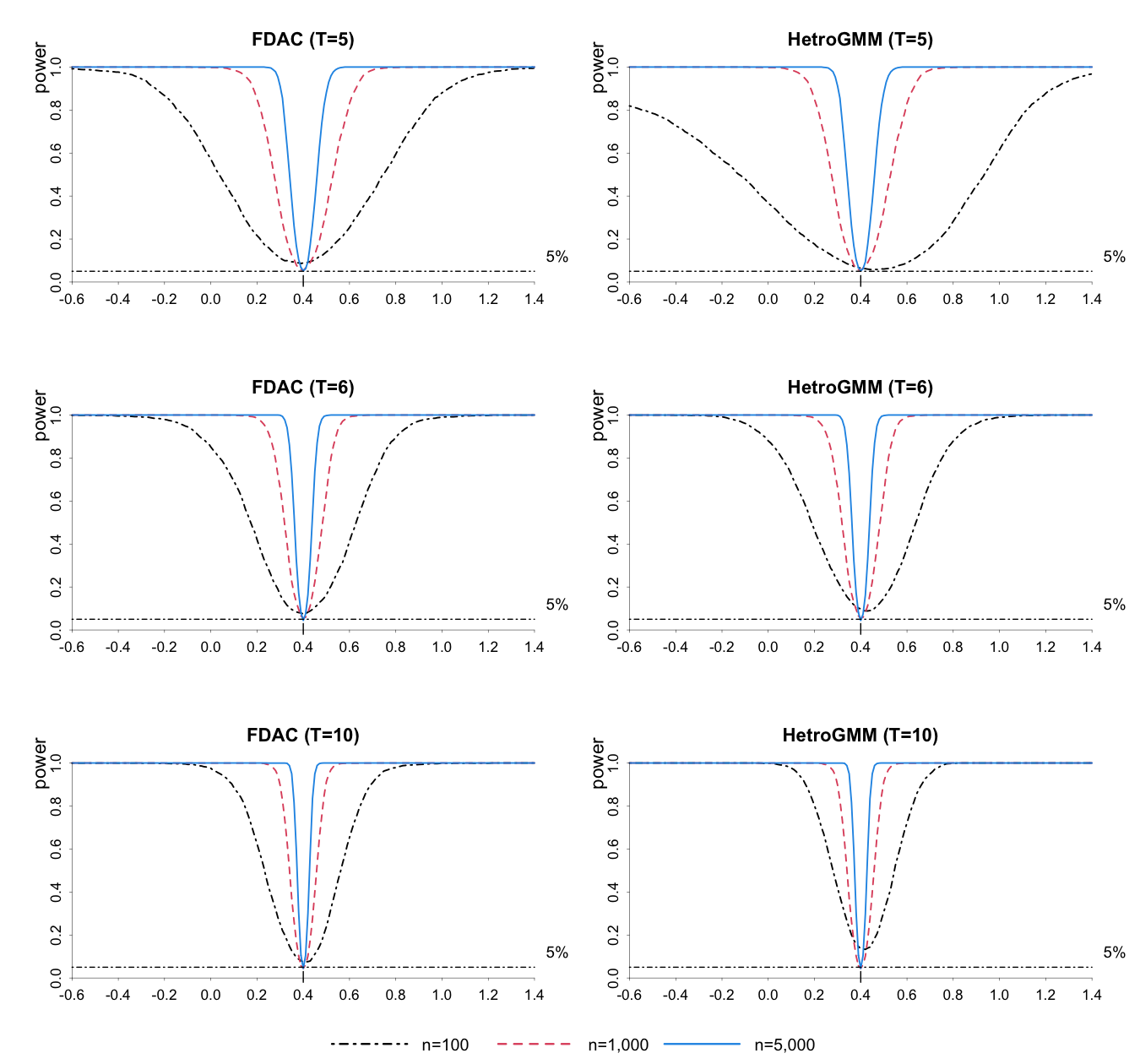
Figure S.1: Empirical power functions for FDAC and HetroGMM estimators of $E(\phi_{i})=0.4$ in a heterogeneous AR(1) panel where $\phi_{i}$ is uniformly distributed, $\phi_{i}=\mu_{\phi}+v_{i}$, $\mu_{\phi}=E(\phi_{i})=0.4$, and $v_{i}\sim IIDU(-0.5,0.5)$, with Gaussian errors and GARCH effects

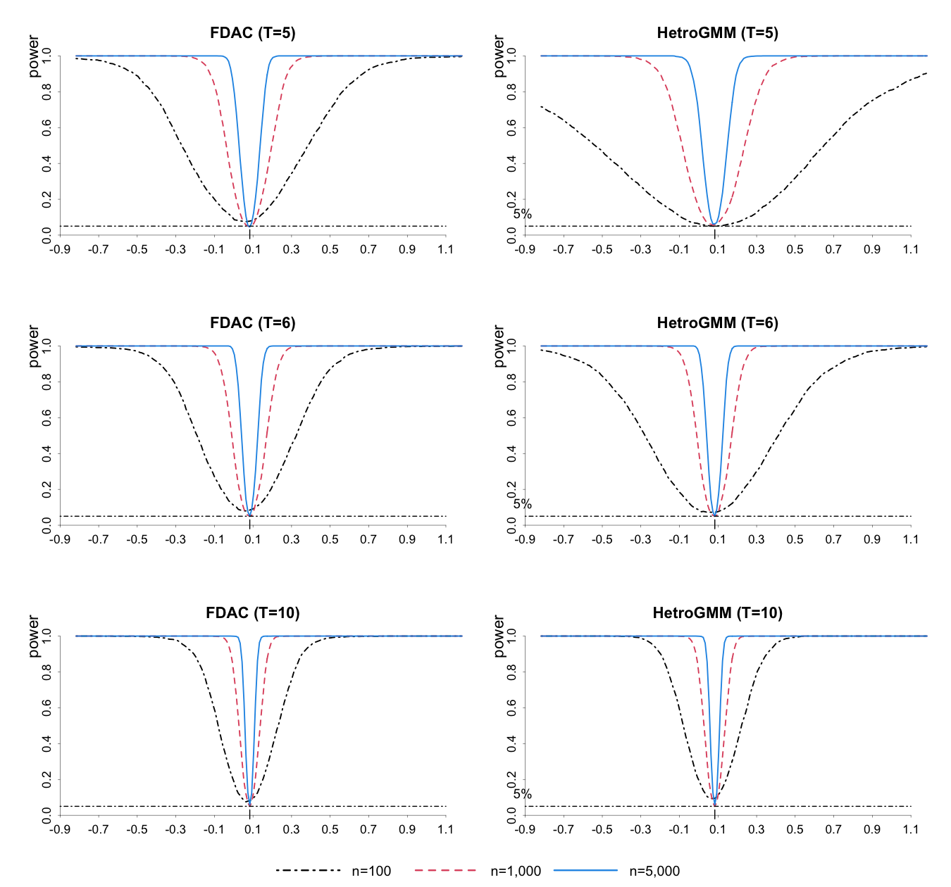
Figure S.2: Empirical power functions for FDAC and HetroGMM estimators of $Var(\phi_{i})=0.083$ in a heterogeneous AR(1) panel where $\phi_{i}$ is uniformly distributed, $\phi_{i}=\mu_{\phi}+v_{i}$, $\mu_{\phi}=E(\phi_{i})=0.4$, and $v_{i}\sim IIDU(-0.5,0.5)$, with Gaussian errors and GARCH effects

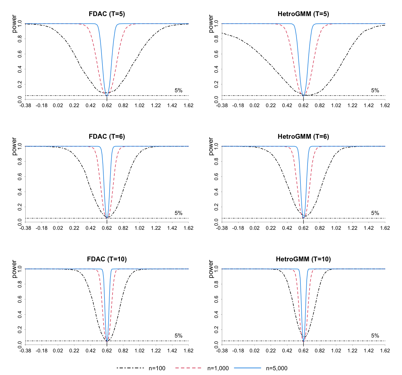
Figure S.3: Empirical power functions for FDAC and HetroGMM estimators of $E(\phi_{i})=0.62$ in a heterogeneous panel AR(1) model where $\phi_{i}$ is categorical distributed with Gaussian errors and GARCH effects

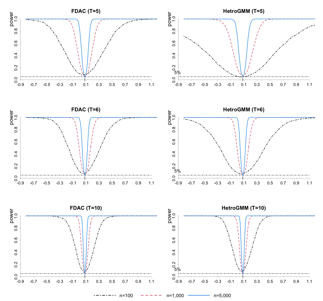
Figure S.4: Empirical power functions for FDAC and HetroGMM estimators of $Var(\phi_{i})=0.076$ in a heterogeneous panel AR(1) model where $\phi_{i}$ is categorical distributed with Gaussian errors and GARCH effects

S.4.2 Simulation results of FDAC, FDLS, AH, AAH, AB, and BB estimators with non-Gaussian errors

Tables S.3–S.5 report bias, RMSE, and size of the FDAC, FDLS, AH, AAH, AB, and BB estimators with $\phi_{i}=\mu_{\phi}+v_{i}$, $v_{i}\sim IIDU(-a,a)$, $\mu_{\phi}=0.4$, and $a\in\{0,0.3,0.5\}$, under non-Gaussian errors and with GARCH effects.

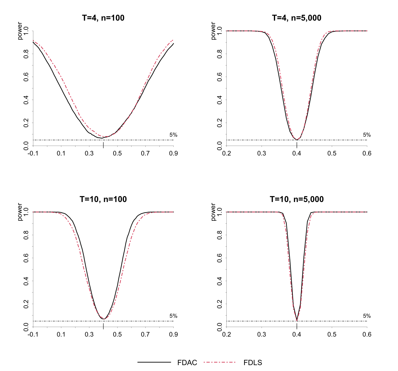
Figure S.5: Empirical power functions for FDAC and FDLS estimators of $\phi_{0}=0.4$ in a homogeneous AR(1) panel with Gaussian errors and GARCH effects

Table S.3: Bias, RMSE, and size of FDAC, FDLS, AH, AAH, AB, and BB estimators of $\phi$ $(\phi_{0}=0.4)$ in a homogeneous panel AR(1) model with non-Gaussian errors and GARCH effects

			Bias							RMSE							Size ($\times 100$)
$T$	$n$		FDAC	FDLS	AH	AAH	AB	BB		FDAC	FDLS	AH	AAH	AB	BB		FDAC	FDLS	AH	AAH	AB	BB
4	100		-0.023	-0.006	1.447	0.042	-0.085	-0.002		0.281	0.240	62.477	0.305	0.348	0.174		12.7	10.2	10.3	16.1	17.2	24.4
4	1,000		-0.002	0.000	0.068	0.055	-0.016	-0.005		0.111	0.097	1.126	0.211	0.109	0.070		5.8	6.6	7.0	14.4	8.2	10.9
4	5,000		0.002	0.000	0.014	0.029	-0.005	-0.002		0.059	0.056	0.373	0.151	0.054	0.035		5.2	5.8	5.7	10.7	7.1	6.5
6	100		-0.006	-0.002	-0.086	0.008	-0.079	0.001		0.161	0.168	0.232	0.160	0.183	0.118		8.6	10.2	26.8	35.2	32.0	41.0
6	1,000		-0.001	-0.002	-0.012	0.001	-0.015	-0.004		0.064	0.068	0.084	0.063	0.057	0.039		5.3	5.8	10.2	12.8	10.8	12.7
6	5,000		0.000	-0.001	-0.004	-0.001	-0.006	-0.002		0.032	0.035	0.042	0.027	0.029	0.020		4.4	5.1	6.5	8.0	8.0	7.6
10	100		-0.006	-0.004	-0.060	0.000	-0.057	-0.009		0.109	0.121	0.116	0.108	0.107	0.080		8.6	9.8	57.1	70.7	61.9	69.7
10	1,000		-0.001	-0.002	-0.012	-0.005	-0.014	-0.007		0.041	0.047	0.036	0.030	0.032	0.024		5.3	6.1	16.6	24.0	19.6	23.2
10	5,000		-0.001	0.000	-0.005	-0.003	-0.007	-0.004		0.021	0.024	0.019	0.015	0.016	0.012		4.6	4.7	8.8	12.2	11.8	12.2

Notes: The DGP is given by $y_{it}=\mu_{i}(1-\phi_{i})+\phi_{i}y_{i,t-1}+u_{it}$ for $i=1,2,...,n$, and $t=-50,-49,...,T$ with $\mu_{i}=\alpha_{i}/(1-\phi_{i})$, where errors, $u_{it}=h_{it}\varepsilon_{it}$, are generated to be non-Gaussian distributed and cross-sectionally heteroskedastic with GARCH effects: $\varepsilon_{it}=\left(e_{it}-2\right)/2$, where $e_{it}\sim IID\chi_{2}^{2}$ and $\chi_{2}^{2}$ is a chi-squared variate with two degrees of freedom, and $h_{it}^{2}=\sigma_{i}^{2}(1-\psi_{0}-\psi_{1})+\psi_{0}h_{i,t-1}^{2}+\psi_{1}u_{i,t-1}^{2}$ with $\sigma_{i}^{2}\sim IID(0.5+0.5z_{i}^{2})$, $z_{i}\sim IIDN(0,1)$, $\psi_{0}=0.6$, and $\psi_{1}=0.2$. The initial values are given by $y_{i,-51}=0$, $\varepsilon_{i,-51}=0$, and $h_{i,-51}=0$. The homogeneous AR(1) coefficients are generated as $\phi_{i}=\phi$ for $i=1,2,...,n$ with $\phi_{0}=0.4$. For each experiment, $(\alpha_{i},\sigma_{i})^{\prime}$ are generated differently across replications. The FDAC estimator is calculated by (6.1), and its asymptotic variance is estimated by the Delta method. “FDLS” denotes the first-difference least square estimator proposed by Han and Phillips (2010). “AH”, “AAH”, “AB”, and “BB” denote the 2-step GMM estimators proposed by Anderson and Hsiao (1981, 1982), Chudik and Pesaran (2021), Arellano and Bond (1991), and Blundell and Bond (1998). The estimation is based on $\{y_{i1},y_{i2},...,y_{iT}\}$ for $i=1,2,...,n$. The nominal size of the tests is set to 5 per cent. The number of replications is $2,000$.

Table S.4: Bias, RMSE, and size of FDAC, FDLS, AH, AAH, AB, and BB estimators in a heterogeneous panel AR(1) model where $\phi_{i}=\mu_{\phi}+v_{i}$ and $v_{i}\sim IIDU(-0.3,0.3)$ with $\mu_{\phi}=0.4$, non-Gaussian errors, and GARCH effects

			Bias							RMSE							Size ($\times 100$)
$T$	$n$		FDAC	FDLS	AH	AAH	AB	BB		FDAC	FDLS	AH	AAH	AB	BB		FDAC	FDLS	AH	AAH	AB	BB
4	100		-0.023	-0.024	-57.795	0.020	-0.127	-0.005		0.284	0.244	2590.301	0.305	0.420	0.190		12.9	11.1	12.0	18.1	19.4	26.7
4	1,000		-0.003	-0.022	-0.035	0.014	-0.042	-0.020		0.112	0.100	0.452	0.189	0.137	0.078		6.3	6.6	12.4	15.7	11.1	12.2
4	5,000		0.002	-0.022	-0.061	-0.015	-0.026	-0.017		0.060	0.060	0.295	0.112	0.065	0.041		5.4	8.8	14.5	14.5	11.2	11.3
6	100		-0.005	-0.022	-0.130	-0.006	-0.109	-0.002		0.168	0.176	0.261	0.159	0.210	0.133		9.2	10.3	33.1	34.2	37.0	44.7
6	1,000		-0.001	-0.024	-0.058	-0.011	-0.038	-0.013		0.066	0.074	0.104	0.055	0.074	0.044		5.1	8.1	20.0	12.4	17.6	14.2
6	5,000		0.000	-0.023	-0.051	-0.011	-0.026	-0.009		0.033	0.043	0.067	0.031	0.041	0.024		4.1	13.5	28.9	9.8	18.1	11.1
10	100		-0.005	-0.024	-0.083	-0.012	-0.075	-0.007		0.116	0.129	0.138	0.114	0.127	0.096		9.3	10.2	62.2	69.7	66.1	72.2
10	1,000		-0.002	-0.024	-0.034	-0.008	-0.027	-0.007		0.044	0.055	0.052	0.034	0.044	0.028		5.7	9.4	30.5	20.8	28.1	21.2
10	5,000		-0.001	-0.022	-0.026	-0.002	-0.017	0.000		0.022	0.034	0.034	0.016	0.025	0.014		4.3	20.2	37.4	9.0	25.4	10.0

Notes: The DGP is given by $y_{it}=\mu_{i}(1-\phi_{i})+\phi_{i}y_{i,t-1}+u_{it}$ for $i=1,2,...,n$, and $t=-50,-49,...,T$ with $\mu_{i}=\alpha_{i}/(1-\phi_{i})$ featuring non-Gaussian errors with GARCH effects. The heterogeneous AR(1) coefficients are generated as case (a): $\phi_{i}=\mu_{\phi}+v_{i}$ and $v_{i}\sim IIDU(-a,a)$ with $\mu_{\phi}=0.4$ and $a=0.3$. For each experiment, $(\alpha_{i},\phi_{i},\sigma_{i})^{\prime}$ are generated differently across replications. The FDAC estimator is calculated by (6.1), and its asymptotic variance is estimated by the Delta method. “FDLS” denotes the first-difference least square estimator proposed by Han and Phillips (2010). “AH”, “AAH”, “AB”, and “BB” denote the 2-step GMM estimators proposed by Anderson and Hsiao (1981, 1982), Chudik and Pesaran (2021), Arellano and Bond (1991), and Blundell and Bond (1998). The estimation is based on $\{y_{i1},y_{i2},...,y_{iT}\}$ for $i=1,2,...,n$. The nominal size of the tests is set to 5 per cent. The number of replications is $2,000$. See also the notes to Table S.3.

Table S.5: Bias, RMSE, and size of FDAC, FDLS, AH, AAH, AB, and BB estimators in a heterogeneous panel AR(1) model where $\phi_{i}=\mu_{\phi}+v_{i}$ and $v_{i}\sim IIDU(-0.5,0.5)$ with $\mu_{\phi}=0.4$, non-Gaussian errors, and GARCH effects

			Bias							RMSE							Size ($\times 100$)
$T$	$n$		FDAC	FDLS	AH	AAH	AB	BB		FDAC	FDLS	AH	AAH	AB	BB		FDAC	FDLS	AH	AAH	AB	BB
4	100		-0.022	-0.059	3.092	-0.020	-0.214	0.012		0.289	0.255	123.889	0.299	0.628	0.242		12.2	12.3	18.0	21.1	24.0	35.0
4	1,000		-0.004	-0.062	-0.160	-0.053	-0.117	-0.052		0.115	0.119	0.623	0.159	0.202	0.103		6.8	12.9	24.8	22.5	22.5	19.4
4	5,000		0.002	-0.062	-0.182	-0.073	-0.097	-0.054		0.060	0.084	0.238	0.100	0.125	0.069		5.3	31.9	48.9	40.4	35.4	31.5
6	100		-0.005	-0.059	-0.211	-0.030	-0.179	0.015		0.178	0.193	0.314	0.165	0.273	0.174		9.5	12.7	44.0	35.2	47.8	54.5
6	1,000		-0.001	-0.064	-0.147	-0.034	-0.113	-0.036		0.071	0.097	0.172	0.064	0.138	0.063		5.6	20.8	53.2	17.8	47.4	25.0
6	5,000		0.000	-0.063	-0.141	-0.035	-0.101	-0.032		0.035	0.073	0.148	0.043	0.110	0.042		3.9	55.3	90.3	34.3	79.1	36.9
10	100		-0.005	-0.061	-0.139	-0.038	-0.121	0.019		0.128	0.150	0.190	0.131	0.173	0.136		9.7	14.2	73.8	69.5	75.9	80.7
10	1,000		-0.002	-0.064	-0.097	-0.031	-0.082	-0.022		0.049	0.084	0.108	0.051	0.093	0.044		5.6	30.8	77.0	33.0	72.0	34.9
10	5,000		-0.001	-0.062	-0.089	-0.025	-0.073	-0.012		0.025	0.068	0.093	0.033	0.077	0.023		4.9	77.2	98.0	36.6	94.2	23.1

Notes: The DGP is given by $y_{it}=\mu_{i}(1-\phi_{i})+\phi_{i}y_{i,t-1}+u_{it}$ for $i=1,2,...,n$, and $t=-50,-49,...,T$ with $\mu_{i}=\alpha_{i}/(1-\phi_{i})$ featuring non-Gaussian errors with GARCH effects. The heterogeneous AR(1) coefficients are generated as case (a): $\phi_{i}=\mu_{\phi}+v_{i}$ and $v_{i}\sim IIDU(-a,a)$ with $\mu_{\phi}=0.4$ and $a=0.5$. For each experiment, $(\alpha_{i},\phi_{i},\sigma_{i})^{\prime}$ are generated differently across replications. The FDAC estimator is calculated by (6.1), and its asymptotic variance is estimated by the Delta method. “FDLS” denotes the first-difference least square estimator proposed by Han and Phillips (2010). “AH”, “AAH”, “AB”, and “BB” denote the 2-step GMM estimators proposed by Anderson and Hsiao (1981, 1982), Chudik and Pesaran (2021), Arellano and Bond (1991), and Blundell and Bond (1998). The estimation is based on $\{y_{i1},y_{i2},...,y_{iT}\}$ for $i=1,2,...,n$. The nominal size of the tests is set to 5 per cent. The number of replications is $2,000$. See also the notes to Table S.3.

S.4.3 Simulation results of FDAC and MSW estimators

Table S.6 reports bias, RMSE, and size of the FDAC and MSW estimators in homogeneous panels with $\phi_{i}=\phi$ for all $i$.

Table S.6: Bias, RMSE, and size of FDAC and MSW estimators of $\phi$ in homogeneous panels with Gaussian errors and GARCH effects

		Bias			RMSE			Size ($\times 100$)
$T$	$n$	FDAC	MSW		FDAC	MSW		FDAC	MSW
$\phi_{i}=\mu_{\phi}=0.475$ for all $i$
6	100	0.004	-0.045		0.098	0.087		7.9	9.1
6	1,000	0.000	-0.037		0.030	0.045		4.1	35.8
10	100	0.003	-0.028		0.064	0.086		6.5	7.1
10	1,000	0.000	-0.024		0.020	0.036		4.2	17.0
$\phi_{i}=\mu_{\phi}=0.620$ for all $i$
6	100	0.003	0.094		0.095	0.143		7.9	12.0
6	1,000	0.000	0.096		0.029	0.102		4.5	78.1
10	100	0.003	0.125		0.062	0.169		5.5	18.7
10	1,000	0.000	0.123		0.019	0.129		4.3	92.2

Notes: The DGP is given by $y_{it}=\mu_{i}(1-\phi_{i})+\phi_{i}y_{i,t-1}+u_{it}$ for $i=1,2,...,n$, and $t=-50,-49,...,T$ with $\mu_{i}=\alpha_{i}/(1-\phi_{i})$ featuring Gaussian errors with GARCH effects. The homogeneous AR(1) coefficients are generated as $\phi_{i}=\phi$ for all $i$ with $\phi_{0}\in\{0.475,0.62\}$. For each experiment, $(\alpha_{i},\sigma_{i})^{\prime}$ are generated differently across replications. The FDAC estimator is calculated based on (6.1), and its asymptotic variance is estimated by the Delta method. “MSW” denotes the kernel-weighting likelihood estimator proposed by Mavroeidis et al. (2015) and calculated based on an assumption that $(\alpha_{i},\phi_{i})|y_{i1}$ follows a multivariate normal distribution $N(\boldsymbol{\mu},\boldsymbol{V})$ with initial values given by $\boldsymbol{\mu}=(5,0.5)$, $\sigma_{\alpha}=2$, $\sigma_{\phi}=0.4$, $corr(\alpha_{i},\phi_{i})=0.5$ with $\sigma_{u}=0.5$. The nominal size of the tests is set to 5 per cent. The number of replications is $1,000$.

S.4.4 Simulation results with different initialization

Table S.7 reports the bias, RMSE, and size of the FDAC and MSW estimators in heterogeneous panels ($a=0.3$) for different degrees of non-stationarity of initialization $M=1,2,51$. Tables S.8–S.10 report the bias, RMSE, and sizes of the FDAC, FDLS, AH, AAH, AB, and BB estimators in homogeneous panels for $M=1,2$ and 15, and $\kappa^{2}\in\{1,3,5\}$. The simulation results for heterogeneous panels with $\phi_{i}=\mu_{\phi}+v_{i}$, $\mu_{\phi}=0.4$, and $v_{i}\sim IIDU(-a,a)$ are shown in Tables S.11–S.13 for $a=0.3$, and Tables S.14–S.16 for $a=0.5$.

Table S.7: Bias, RMSE, and size of FDAC and MSW estimators in a heterogeneous panel AR(1) model for different degrees of non-stationarity of initialization $M=1,2,51$ with $\phi_{i}=\mu_{\phi}+v_{i}$, $\mu_{\phi}=0.4$, and $v_{i}\sim IIDU(-0.3,0.3)$

				FDAC				MSW
	$T$	$n/M$		1	2	51		1	2	51
	4	100		0.072	0.026	-0.004		-0.054	-0.042	-0.002
	4	1,000		0.078	0.035	0.002		-0.045	-0.036	0.002
Bias	6	100		0.045	0.018	0.000		-0.062	-0.040	0.008
	6	1,000		0.045	0.018	0.001		-0.053	-0.029	0.021
	10	100		0.022	0.007	-0.002		-0.067	-0.036	0.019
	10	1,000		0.023	0.008	-0.001		-0.063	-0.032	0.022
	4	100		0.203	0.194	0.193		0.083	0.082	0.085
	4	1,000		0.099	0.070	0.062		0.051	0.042	0.030
RMSE	6	100		0.130	0.124	0.123		0.086	0.080	0.086
	6	1,000		0.060	0.044	0.040		0.057	0.037	0.035
	10	100		0.086	0.084	0.084		0.093	0.083	0.092
	10	1,000		0.036	0.029	0.028		0.066	0.040	0.036
	4	100		9.9	9.2	7.7		21.3	14.6	8.0
	4	1,000		26.9	7.0	6.2		73.2	44.5	10.8
Size $(\times 100)$	6	100		11.8	8.3	7.1		21.4	10.7	6.5
	6	1,000		24.4	8.9	5.2		80.0	29.3	14.5
	10	100		7.2	5.5	5.5		20.4	9.2	6.2
	10	1,000		14.5	6.6	5.8		84.8	30.7	13.6

Notes: The DGP is given by $y_{it}=\mu_{i}(1-\phi_{i})+\phi_{i}y_{i,t-1}+u_{it}$ for $i=1,2,...,n$, and $t=1,2,...,T$ with $\mu_{i}=\alpha_{i}/(1-\phi_{i})$ featuring Gaussian errors with GARCH effects. The heterogeneous AR(1) coefficients are generated as case (a): $\phi_{i}=\mu_{\phi}+v_{i}$ and $v_{i}\sim IIDU(-a,a)$ with $\mu_{\phi}=0.4$ and $a=0.3$. The initial values are generated as $y_{i1}\sim IIDN\left(\mu_{i}(1-\phi_{i}^{M}),\sigma_{i}^{2}(1-\phi_{i}^{2M})/(1-\phi_{i}^{2})\right)$ with $M=1,2$ for the non-stationary case and $M=51$ for the stationary case. The FDAC estimator is calculated based on (6.1), and its asymptotic variance is estimated by the Delta method. “MSW” denotes the kernel-weighting likelihood estimator by Mavroeidis et al. (2015). The number of replications is $1,000$. See also the notes to Table S.6.

Table S.8: Bias of FDAC, FDLS, AH, AAH, AB, and BB estimators of $\phi_{0}=0.4$ in a homogeneous panel AR(1) model for different degrees of non-stationarity of initialization $M$ and $\kappa^{2}=Var(\alpha_{i})/Var(u_{it})$

				Bias
				FDAC				FDLS				AH				AAH				AB				BB
	$T$	$n/\kappa^{2}$		1	3	5		1	3	5		1	3	5		1	3	5		1	3	5		1	3	5
	4	100		0.016	0.053	0.088		0.012	0.041	0.069		1.709	0.125	0.419		0.100	0.104	0.109		-0.050	-0.118	-0.118		0.151	0.320	0.399
	4	1,000		0.015	0.052	0.087		0.010	0.038	0.065		0.009	0.010	0.012		0.050	0.049	0.051		-0.005	-0.013	-0.013		0.165	0.334	0.401
	4	5,000		0.015	0.052	0.087		0.011	0.040	0.067		0.004	0.004	0.005		0.003	0.003	0.002		0.000	0.000	-0.002		0.169	0.335	0.401
	6	100		0.008	0.028	0.047		0.008	0.023	0.037		-0.049	-0.053	-0.057		0.023	0.024	0.024		-0.054	-0.078	-0.077		0.091	0.246	0.351
$M=1$	6	1,000		0.006	0.026	0.045		0.005	0.020	0.034		-0.004	-0.005	-0.005		0.000	0.000	0.000		-0.006	-0.008	-0.008		0.094	0.270	0.381
	6	5,000		0.008	0.027	0.046		0.006	0.020	0.035		0.000	-0.001	-0.001		0.000	0.000	0.000		-0.001	-0.001	-0.002		0.096	0.276	0.386
	10	100		0.005	0.015	0.026		0.004	0.012	0.019		-0.033	-0.034	-0.036		0.007	0.006	0.006		-0.035	-0.040	-0.040		0.034	0.112	0.200
	10	1,000		0.003	0.013	0.023		0.003	0.010	0.017		-0.004	-0.004	-0.004		0.000	0.000	0.000		-0.004	-0.005	-0.005		0.033	0.092	0.187
	10	5,000		0.004	0.014	0.024		0.003	0.010	0.018		0.000	-0.001	-0.001		0.000	0.000	0.000		0.000	-0.001	-0.001		0.034	0.094	0.192
	4	100		0.004	0.010	0.016		0.003	0.008	0.013		-0.034	1.696	1.750		0.098	0.100	0.102		-0.036	-0.079	-0.097		0.061	0.153	0.223
	4	1,000		0.003	0.009	0.015		0.001	0.006	0.010		0.008	0.008	0.009		0.052	0.051	0.049		-0.004	-0.008	-0.011		0.061	0.162	0.244
	4	5,000		0.003	0.009	0.015		0.003	0.007	0.012		0.003	0.003	0.004		0.004	0.003	0.003		0.000	0.000	0.000		0.063	0.168	0.252
	6	100		0.001	0.005	0.008		0.003	0.006	0.008		-0.049	-0.049	-0.050		0.022	0.023	0.023		-0.046	-0.066	-0.072		0.036	0.099	0.162
$M=2$	6	1,000		0.000	0.003	0.007		0.001	0.003	0.006		-0.004	-0.004	-0.004		0.000	0.000	0.000		-0.005	-0.007	-0.008		0.027	0.068	0.126
	6	5,000		0.002	0.005	0.008		0.001	0.004	0.006		0.000	0.000	0.000		0.000	0.000	0.000		0.000	-0.001	-0.001		0.027	0.067	0.125
	10	100		0.002	0.004	0.005		0.002	0.003	0.004		-0.033	-0.033	-0.033		0.006	0.006	0.007		-0.033	-0.037	-0.039		0.015	0.051	0.092
	10	1,000		0.000	0.002	0.003		0.001	0.002	0.003		-0.004	-0.004	-0.004		0.000	0.000	0.000		-0.004	-0.005	-0.005		0.009	0.019	0.032
	10	5,000		0.001	0.002	0.004		0.001	0.002	0.003		0.000	0.000	0.000		0.000	0.000	0.000		0.000	-0.001	-0.001		0.009	0.018	0.028
	4	100		0.002	0.002	0.002		0.001	0.001	0.001		0.202	0.202	0.202		0.100	0.100	0.100		-0.030	-0.053	-0.064		0.015	0.046	0.074
	4	1,000		0.001	0.001	0.001		-0.001	-0.001	-0.001		0.008	0.008	0.008		0.051	0.051	0.051		-0.003	-0.005	-0.007		0.002	0.008	0.011
	4	5,000		0.000	0.000	0.000		0.001	0.001	0.001		0.003	0.003	0.003		0.004	0.004	0.004		0.000	0.000	0.000		0.001	0.003	0.003
	6	100		0.000	0.000	0.000		0.002	0.002	0.002		-0.049	-0.049	-0.049		0.022	0.022	0.022		-0.041	-0.055	-0.061		0.012	0.038	0.066
$M=15$	6	1,000		-0.001	-0.001	-0.001		0.000	0.000	0.000		-0.004	-0.004	-0.004		0.000	0.000	0.000		-0.004	-0.006	-0.006		0.001	0.003	0.004
	6	5,000		0.000	0.000	0.000		0.000	0.000	0.000		0.000	0.000	0.000		0.000	0.000	0.000		0.000	-0.001	-0.001		0.001	0.001	0.001
	10	100		0.001	0.001	0.001		0.001	0.001	0.001		-0.033	-0.033	-0.033		0.006	0.006	0.006		-0.031	-0.035	-0.036		0.007	0.030	0.055
	10	1,000		-0.001	-0.001	-0.001		0.000	0.000	0.000		-0.004	-0.004	-0.004		0.000	0.000	0.000		-0.003	-0.004	-0.004		0.001	0.001	0.002
	10	5,000		0.000	0.000	0.000		0.000	0.000	0.000		0.000	0.000	0.000		0.000	0.000	0.000		0.000	0.000	0.000		0.000	0.000	0.000

Notes: The DGP is given by $y_{it}=\alpha_{i}+\phi_{i}y_{i,t-1}+u_{it}$ for $i=1,2,...,n$ and $t=1,2,...,T$ with Gaussian errors, where $\phi_{i}=0.4$ for all $i$, and $y_{i0}\sim IIDN\left(\mu_{i}(1-\phi_{i}^{M}),\sigma_{i}^{2}(1-\phi_{i}^{2M})/(1-\phi_{i}^{2})\right)$. $\kappa^{2}=Var(\alpha_{i})/Var(u_{it})\in\{1,3,5\}$. The number of replications is $2,000$. See also the notes to Table S.3.

Table S.9: RMSE of FDAC, FDLS, AH, AAH, AB, and BB estimators of $\phi_{0}=0.4$ in a homogeneous panel AR(1) model for different degrees of non-stationarity of initialization $M$ and $\kappa^{2}=Var(\alpha_{i})/Var(u_{it})$

				RMSE
				FDAC				FDLS				AH				AAH				AB				BB
	$T$	$n/\kappa^{2}$		1	3	5		1	3	5		1	3	5		1	3	5		1	3	5		1	3	5
	4	100		0.166	0.172	0.185		0.147	0.152	0.161		53.877	3.134	6.250		0.308	0.307	0.309		0.340	0.572	0.455		0.207	0.338	0.406
	4	1,000		0.056	0.074	0.102		0.048	0.060	0.080		0.160	0.171	0.184		0.185	0.185	0.189		0.102	0.160	0.141		0.172	0.335	0.402
	4	5,000		0.028	0.057	0.090		0.024	0.045	0.070		0.069	0.073	0.078		0.050	0.047	0.044		0.044	0.072	0.062		0.170	0.335	0.401
	6	100		0.099	0.102	0.108		0.101	0.103	0.107		0.177	0.185	0.193		0.143	0.145	0.146		0.157	0.189	0.184		0.141	0.271	0.362
$M=1$	6	1,000		0.033	0.041	0.055		0.033	0.038	0.047		0.056	0.058	0.060		0.029	0.028	0.027		0.047	0.058	0.056		0.100	0.273	0.382
	6	5,000		0.016	0.031	0.049		0.016	0.025	0.038		0.025	0.026	0.027		0.013	0.013	0.012		0.021	0.026	0.025		0.097	0.277	0.386
	10	100		0.066	0.067	0.070		0.073	0.074	0.075		0.089	0.091	0.093		0.067	0.065	0.064		0.087	0.095	0.095		0.073	0.138	0.220
	10	1,000		0.021	0.024	0.031		0.024	0.026	0.029		0.026	0.026	0.027		0.016	0.016	0.016		0.024	0.026	0.026		0.038	0.096	0.191
	10	5,000		0.010	0.017	0.026		0.011	0.014	0.020		0.011	0.011	0.011		0.007	0.007	0.007		0.010	0.011	0.011		0.035	0.095	0.193
	4	100		0.167	0.167	0.167		0.146	0.147	0.147		10.797	66.506	97.482		0.306	0.307	0.309		0.296	0.419	0.520		0.161	0.224	0.275
	4	1,000		0.054	0.055	0.056		0.047	0.047	0.048		0.158	0.159	0.161		0.189	0.186	0.184		0.087	0.126	0.146		0.080	0.173	0.250
	4	5,000		0.024	0.026	0.029		0.021	0.022	0.024		0.068	0.068	0.069		0.051	0.051	0.050		0.038	0.056	0.065		0.067	0.170	0.253
	6	100		0.099	0.099	0.099		0.100	0.101	0.101		0.175	0.176	0.177		0.142	0.142	0.143		0.144	0.173	0.180		0.105	0.156	0.209
$M=2$	6	1,000		0.032	0.032	0.033		0.033	0.033	0.033		0.055	0.056	0.056		0.029	0.029	0.029		0.044	0.052	0.055		0.041	0.080	0.137
	6	5,000		0.014	0.015	0.016		0.015	0.015	0.016		0.025	0.025	0.025		0.013	0.013	0.013		0.020	0.023	0.025		0.031	0.070	0.128
	10	100		0.066	0.066	0.066		0.073	0.073	0.073		0.088	0.088	0.089		0.066	0.066	0.066		0.084	0.091	0.093		0.062	0.085	0.121
	10	1,000		0.021	0.021	0.021		0.023	0.023	0.024		0.026	0.026	0.026		0.016	0.016	0.016		0.023	0.025	0.026		0.019	0.026	0.038
	10	5,000		0.009	0.010	0.010		0.010	0.010	0.011		0.011	0.011	0.011		0.007	0.007	0.007		0.010	0.011	0.011		0.012	0.020	0.030
	4	100		0.167	0.167	0.167		0.146	0.146	0.146		4.182	4.182	4.182		0.308	0.308	0.308		0.269	0.336	0.372		0.145	0.173	0.198
	4	1,000		0.054	0.054	0.054		0.047	0.047	0.047		0.157	0.157	0.157		0.186	0.186	0.186		0.079	0.100	0.111		0.048	0.054	0.059
	4	5,000		0.024	0.024	0.024		0.021	0.021	0.021		0.068	0.068	0.068		0.051	0.051	0.051		0.034	0.044	0.049		0.022	0.025	0.027
	6	100		0.099	0.099	0.099		0.100	0.100	0.100		0.174	0.174	0.174		0.142	0.142	0.142		0.136	0.157	0.164		0.094	0.113	0.134
$M=15$	6	1,000		0.032	0.032	0.032		0.032	0.032	0.032		0.055	0.055	0.055		0.029	0.029	0.029		0.041	0.047	0.049		0.028	0.029	0.030
	6	5,000		0.014	0.014	0.014		0.015	0.015	0.015		0.025	0.025	0.025		0.013	0.013	0.013		0.019	0.021	0.022		0.013	0.013	0.013
	10	100		0.066	0.066	0.066		0.073	0.073	0.073		0.088	0.088	0.088		0.066	0.066	0.066		0.081	0.087	0.089		0.059	0.070	0.088
	10	1,000		0.021	0.021	0.021		0.023	0.023	0.023		0.026	0.026	0.026		0.016	0.016	0.016		0.022	0.024	0.025		0.016	0.016	0.017
	10	5,000		0.009	0.009	0.009		0.010	0.010	0.010		0.011	0.011	0.011		0.007	0.007	0.007		0.010	0.010	0.011		0.007	0.007	0.007

Notes: $\kappa^{2}=Var(\alpha_{i})/Var(u_{it})$ with $\kappa^{2}\in\{1,3,5\}$. See also the notes to Table S.8.

Table S.10: Size of FDAC, FDLS, AH, AAH, AB, and BB estimators of $\phi_{0}=0.4$ in a homogeneous panel AR(1) model for different degrees of non-stationarity of initialization $M$ and $\kappa^{2}=Var(\alpha_{i})/Var(u_{it})$

				Size $(\times 100)$
				FDAC				FDLS				AH				AAH				AB				BB
	$T$	$n/\kappa^{2}$		1	3	5		1	3	5		1	3	5		1	3	5		1	3	5		1	3	5
	4	100		7.3	8.2	9.7		7.0	8.1	11.3		7.1	6.8	7.0		15.7	15.4	15.3		10.7	13.1	11.8		44.0	88.3	98.4
	4	1,000		6.7	16.2	36.3		5.6	13.8	29.2		4.8	4.9	4.9		11.5	11.9	11.8		5.8	6.3	6.0		96.4	100.0	100.0
	4	5,000		9.0	58.5	96.0		8.6	47.0	88.4		4.3	4.3	4.2		5.7	5.6	5.8		5.0	3.9	4.6		100.0	100.0	100.0
	6	100		6.6	7.1	10.4		6.3	7.2	8.7		13.8	13.6	13.6		20.8	21.0	21.0		17.7	18.6	18.8		45.9	86.0	97.6
$M=1$	6	1,000		5.6	14.2	31.7		5.1	9.5	19.0		6.2	6.0	5.6		7.1	6.8	6.6		6.0	6.3	5.8		89.7	100.0	100.0
	6	5,000		8.6	49.5	90.3		7.2	29.0	66.8		5.7	5.7	5.6		5.4	5.7	5.9		5.0	5.6	5.5		100.0	100.0	100.0
	10	100		6.3	7.1	8.7		6.9	7.2	7.7		33.1	32.6	33.1		44.9	44.7	44.5		40.2	40.6	40.3		54.4	82.2	96.4
	10	1,000		5.7	9.7	19.9		6.1	8.1	12.8		7.8	8.1	8.1		9.4	8.9	9.0		8.2	8.3	8.1		60.1	99.2	100.0
	10	5,000		6.6	33.1	74.0		5.2	17.8	40.1		5.0	4.8	4.8		5.9	5.8	5.9		5.1	4.7	4.7		99.3	100.0	100.0
	4	100		7.3	7.4	7.3		6.8	6.6	6.7		6.9	6.9	7.0		15.6	15.4	15.5		9.8	11.7	12.6		22.5	43.9	61.2
	4	1,000		5.9	6.2	6.7		5.0	5.1	5.7		5.0	4.9	4.9		12.0	11.7	11.5		6.0	5.1	5.8		32.6	86.1	98.8
	4	5,000		5.0	6.8	9.2		5.2	6.3	8.8		4.4	4.2	4.2		5.6	5.8	5.7		4.8	4.8	4.7		82.5	100.0	100.0
	6	100		6.3	6.4	6.4		6.4	6.4	6.5		13.7	13.4	13.2		20.6	20.9	20.9		17.1	17.2	18.0		28.7	47.9	65.6
$M=2$	6	1,000		5.3	5.3	5.5		5.4	5.2	5.3		6.2	6.2	6.2		7.2	7.2	7.1		6.3	5.7	6.3		22.8	62.2	89.9
	6	5,000		5.1	6.7	8.9		5.8	6.2	7.3		5.7	5.8	5.8		5.4	5.3	5.4		4.9	4.9	5.1		60.2	98.6	100.0
	10	100		5.7	5.9	6.2		6.6	6.6	6.9		32.9	33.0	32.9		44.6	44.8	44.6		39.5	40.2	40.0		47.8	62.5	76.6
	10	1,000		5.0	5.3	5.7		5.9	5.9	6.1		7.6	7.8	7.8		9.6	9.7	9.6		8.1	8.6	8.2		15.0	30.3	53.3
	10	5,000		4.8	5.1	6.8		4.6	5.1	5.3		5.0	4.9	5.0		5.8	5.9	5.7		5.1	4.6	4.8		27.0	65.4	92.3
	4	100		7.4	7.4	7.4		6.6	6.6	6.6		6.9	6.9	6.9		15.7	15.7	15.7		9.2	10.4	10.9		14.2	21.6	28.2
	4	1,000		5.4	5.4	5.4		5.0	5.0	5.0		4.7	4.7	4.7		11.7	11.7	11.7		6.2	5.8	5.4		6.0	6.6	7.6
	4	5,000		4.8	4.8	4.8		4.6	4.6	4.6		4.5	4.5	4.5		5.7	5.7	5.7		4.8	4.8	5.0		5.3	5.9	5.9
	6	100		6.4	6.4	6.4		6.4	6.4	6.4		13.7	13.7	13.7		20.5	20.5	20.5		16.9	17.1	17.2		24.1	33.8	42.1
$M=15$	6	1,000		5.2	5.2	5.2		5.7	5.7	5.7		6.0	6.0	6.0		7.1	7.1	7.1		6.3	5.9	5.9		7.6	7.8	8.8
	6	5,000		4.9	4.9	4.9		5.8	5.8	5.8		5.8	5.8	5.8		5.8	5.8	5.8		4.8	4.7	5.0		5.7	5.9	6.0
	10	100		5.8	5.8	5.8		6.8	6.8	6.8		33.2	33.2	33.2		44.5	44.5	44.5		39.7	39.6	39.8		46.7	56.6	66.8
	10	1,000		5.1	5.1	5.1		5.9	5.9	5.9		7.6	7.6	7.6		9.4	9.4	9.4		7.9	8.3	8.4		8.9	10.0	10.9
	10	5,000		4.6	4.6	4.6		4.8	4.8	4.8		5.1	5.1	5.1		5.8	5.8	5.8		5.0	4.7	4.6		5.4	5.7	5.8

Notes: $\kappa^{2}=Var(\alpha_{i})/Var(u_{it})$ with $\kappa^{2}\in\{1,3,5\}$. The nominal size of the tests is set to 5 per cent. See also the notes to Table S.8.

Table S.11: Bias of FDAC, FDLS, AH, AAH, AB, and BB estimators in a heterogeneous panel AR(1) model for different degrees of non-stationarity of initialization $M$ and $\kappa^{2}=Var(\alpha_{i})/Var(u_{it})$ with $\phi_{i}=\mu_{\phi}+v_{i}$, $\mu_{\phi}=0.4$, and $v_{i}\sim IIDU(-0.3,0.3)$

				Bias
				FDAC				FDLS				AH				AAH				AB				BB
	$T$	$n/\kappa^{2}$		1.03	3.03	5.03		1.03	3.03	5.03		1.03	3.03	5.03		1.03	3.03	5.03		1.03	3.03	5.03		1.03	3.03	5.03
	4	100		0.081	0.199	0.297		0.034	0.120	0.198		1.243	0.536	1.057		0.075	0.097	0.110		-0.211	-0.081	0.047		0.243	0.422	0.488
	4	1,000		0.078	0.196	0.295		0.029	0.114	0.191		-0.086	-0.138	-0.212		0.007	0.029	0.051		-0.159	0.070	0.170		0.271	0.437	0.491
	4	5,000		0.077	0.195	0.294		0.030	0.115	0.192		-0.091	-0.145	-0.224		-0.008	0.020	0.042		-0.152	0.093	0.181		0.274	0.437	0.491
	6	100		0.045	0.119	0.183		0.011	0.063	0.111		-0.121	-0.169	-0.209		0.020	0.044	0.066		-0.151	-0.099	-0.021		0.158	0.360	0.449
$M=1$	6	1,000		0.044	0.117	0.182		0.008	0.059	0.107		-0.071	-0.107	-0.141		0.007	0.031	0.052		-0.094	-0.016	0.070		0.177	0.414	0.487
	6	5,000		0.045	0.118	0.183		0.008	0.059	0.107		-0.068	-0.102	-0.135		0.007	0.031	0.052		-0.088	-0.007	0.079		0.182	0.422	0.491
	10	100		0.026	0.065	0.102		-0.004	0.023	0.050		-0.072	-0.094	-0.106		0.007	0.019	0.030		-0.082	-0.063	-0.034		0.058	0.199	0.316
	10	1,000		0.023	0.062	0.099		-0.006	0.021	0.047		-0.040	-0.057	-0.067		0.010	0.023	0.035		-0.047	-0.023	0.010		0.057	0.193	0.353
	10	5,000		0.024	0.063	0.100		-0.006	0.021	0.047		-0.037	-0.053	-0.063		0.011	0.025	0.037		-0.043	-0.017	0.017		0.061	0.200	0.363
	4	100		0.034	0.084	0.130		0.002	0.036	0.069		-0.180	-0.031	-0.119		0.069	0.076	0.083		-0.156	-0.189	-0.096		0.137	0.297	0.385
	4	1,000		0.032	0.081	0.128		-0.002	0.032	0.064		-0.072	-0.088	-0.107		0.003	0.009	0.019		-0.111	-0.111	0.026		0.157	0.334	0.413
	4	5,000		0.031	0.081	0.127		-0.001	0.032	0.065		-0.076	-0.093	-0.113		-0.019	-0.006	0.006		-0.105	-0.103	0.043		0.161	0.339	0.415
	6	100		0.018	0.048	0.076		-0.007	0.013	0.033		-0.105	-0.124	-0.143		0.011	0.021	0.031		-0.126	-0.133	-0.101		0.079	0.218	0.322
$M=2$	6	1,000		0.017	0.047	0.075		-0.010	0.010	0.029		-0.060	-0.073	-0.088		-0.003	0.008	0.019		-0.074	-0.069	-0.028		0.077	0.233	0.373
	6	5,000		0.018	0.048	0.076		-0.010	0.010	0.029		-0.056	-0.070	-0.083		-0.003	0.008	0.018		-0.069	-0.063	-0.020		0.079	0.240	0.384
	10	100		0.011	0.027	0.042		-0.014	-0.003	0.007		-0.062	-0.074	-0.083		0.002	0.008	0.012		-0.072	-0.072	-0.062		0.029	0.111	0.198
	10	1,000		0.009	0.024	0.040		-0.015	-0.005	0.005		-0.033	-0.042	-0.049		0.005	0.010	0.016		-0.040	-0.037	-0.025		0.027	0.065	0.152
	10	5,000		0.009	0.025	0.040		-0.016	-0.005	0.005		-0.030	-0.038	-0.045		0.006	0.012	0.017		-0.036	-0.032	-0.019		0.030	0.065	0.151
	4	100		0.001	0.001	0.001		-0.019	-0.019	-0.019		-0.046	-0.046	-0.042		0.063	0.063	0.063		-0.070	-0.070	-0.113		0.005	0.005	0.074
	4	1,000		0.001	0.001	0.001		-0.022	-0.022	-0.022		-0.062	-0.062	-0.062		-0.001	-0.001	-0.001		-0.032	-0.032	-0.054		-0.014	-0.014	-0.009
	4	5,000		0.000	0.000	0.000		-0.021	-0.021	-0.021		-0.067	-0.067	-0.067		-0.027	-0.027	-0.027		-0.027	-0.027	-0.046		-0.017	-0.017	-0.020
	6	100		-0.001	-0.001	-0.001		-0.019	-0.019	-0.019		-0.094	-0.094	-0.094		0.006	0.006	0.006		-0.077	-0.077	-0.102		0.004	0.004	0.068
$M=15$	6	1,000		-0.001	-0.001	-0.001		-0.021	-0.021	-0.021		-0.052	-0.052	-0.052		-0.010	-0.010	-0.010		-0.031	-0.031	-0.046		-0.007	-0.007	-0.007
	6	5,000		0.000	0.000	0.000		-0.021	-0.021	-0.021		-0.049	-0.049	-0.049		-0.010	-0.010	-0.010		-0.026	-0.026	-0.040		-0.007	-0.007	-0.009
	10	100		0.002	0.002	0.002		-0.020	-0.020	-0.020		-0.055	-0.055	-0.055		-0.001	-0.001	-0.001		-0.050	-0.050	-0.059		0.004	0.004	0.066
	10	1,000		0.000	0.000	0.000		-0.021	-0.021	-0.021		-0.028	-0.028	-0.028		0.001	0.001	0.001		-0.020	-0.020	-0.027		0.003	0.003	0.004
	10	5,000		0.000	0.000	0.000		-0.022	-0.022	-0.022		-0.025	-0.025	-0.025		0.002	0.002	0.002		-0.016	-0.016	-0.022		0.005	0.005	0.004

Notes: The DGP is given by $y_{it}=\alpha_{i}+\phi_{i}y_{i,t-1}+u_{it}$ for $t=1,2,...,T$ with Gaussian errors, where $\phi_{i}=0.4+v_{i}$, $v_{i}\sim IIDU(-0.3,0.3)$, and $y_{i0}\sim IIDN\left(\mu_{i}(1-\phi_{i}^{M}),\sigma_{i}^{2}(1-\phi_{i}^{2M})/(1-\phi_{i}^{2})\right)$. $\kappa^{2}=Var(\alpha_{i})/Var(u_{it})\in\{1.03,3.03,5.03\}$. The number of replications is $2,000$. See the notes to Table S.4.

Table S.12: RMSE of FDAC, FDLS, AH, AAH, AB, and BB estimators in a heterogeneous panel AR(1) model for different degrees of non-stationarity of initialization $M$ and $\kappa^{2}=Var(\alpha_{i})/Var(u_{it})$ with $\phi_{i}=\mu_{\phi}+v_{i}$, $\mu_{\phi}=0.4$, and $v_{i}\sim IIDU(-0.3,0.3)$

				RMSE
				FDAC				FDLS				AH				AAH				AB				BB
	$T$	$n/\kappa^{2}$		1.03	3.03	5.03		1.03	3.03	5.03		1.03	3.03	5.03		1.03	3.03	5.03		1.03	3.03	5.03		1.03	3.03	5.03
	4	100		0.187	0.262	0.343		0.156	0.199	0.258		52.302	11.893	57.826		0.280	0.277	0.269		0.464	0.550	0.392		0.284	0.433	0.492
	4	1,000		0.095	0.203	0.300		0.057	0.125	0.198		0.183	0.240	0.358		0.108	0.089	0.101		0.200	0.196	0.205		0.274	0.437	0.492
	4	5,000		0.081	0.196	0.295		0.037	0.117	0.193		0.115	0.167	0.246		0.027	0.031	0.048		0.161	0.124	0.187		0.275	0.437	0.491
	6	100		0.114	0.161	0.215		0.107	0.127	0.161		0.221	0.272	0.321		0.128	0.132	0.145		0.230	0.224	0.189		0.206	0.378	0.456
$M=1$	6	1,000		0.056	0.122	0.186		0.035	0.069	0.113		0.094	0.128	0.161		0.029	0.042	0.058		0.109	0.073	0.095		0.183	0.416	0.488
	6	5,000		0.048	0.119	0.183		0.018	0.061	0.108		0.073	0.107	0.140		0.015	0.034	0.054		0.092	0.034	0.085		0.183	0.422	0.491
	10	100		0.076	0.098	0.128		0.078	0.083	0.096		0.121	0.141	0.154		0.071	0.073	0.077		0.127	0.121	0.109		0.102	0.228	0.332
	10	1,000		0.032	0.067	0.102		0.026	0.033	0.054		0.050	0.066	0.076		0.021	0.030	0.040		0.056	0.040	0.035		0.062	0.199	0.355
	10	5,000		0.026	0.064	0.100		0.012	0.023	0.048		0.039	0.054	0.064		0.014	0.026	0.038		0.045	0.022	0.023		0.062	0.201	0.364
	4	100		0.173	0.190	0.215		0.151	0.158	0.171		10.484	6.444	5.674		0.286	0.280	0.275		0.389	0.550	0.514		0.216	0.333	0.403
	4	1,000		0.063	0.098	0.139		0.049	0.058	0.081		0.169	0.185	0.204		0.126	0.108	0.102		0.154	0.191	0.174		0.167	0.336	0.414
	4	5,000		0.040	0.084	0.129		0.022	0.039	0.068		0.101	0.116	0.135		0.032	0.026	0.025		0.115	0.125	0.089		0.163	0.339	0.415
	6	100		0.106	0.116	0.131		0.105	0.107	0.113		0.204	0.223	0.243		0.130	0.128	0.129		0.203	0.225	0.213		0.147	0.262	0.349
$M=2$	6	1,000		0.038	0.058	0.083		0.035	0.036	0.045		0.083	0.096	0.109		0.029	0.030	0.034		0.090	0.092	0.071		0.088	0.241	0.376
	6	5,000		0.024	0.050	0.078		0.018	0.019	0.033		0.062	0.075	0.088		0.014	0.015	0.022		0.073	0.069	0.036		0.082	0.242	0.385
	10	100		0.072	0.077	0.084		0.079	0.078	0.079		0.113	0.122	0.131		0.071	0.072	0.072		0.117	0.122	0.118		0.081	0.147	0.226
	10	1,000		0.024	0.033	0.046		0.029	0.025	0.026		0.044	0.051	0.058		0.019	0.022	0.025		0.049	0.048	0.040		0.035	0.072	0.160
	10	5,000		0.014	0.027	0.041		0.019	0.012	0.012		0.033	0.040	0.047		0.010	0.014	0.019		0.038	0.035	0.024		0.032	0.067	0.153
	4	100		0.171	0.171	0.171		0.151	0.151	0.151		4.487	4.487	4.398		0.290	0.290	0.290		0.293	0.293	0.391		0.157	0.157	0.217
	4	1,000		0.055	0.055	0.055		0.053	0.053	0.053		0.160	0.160	0.160		0.136	0.136	0.136		0.092	0.092	0.127		0.053	0.053	0.061
	4	5,000		0.025	0.025	0.025		0.030	0.030	0.030		0.093	0.093	0.093		0.038	0.038	0.038		0.047	0.047	0.069		0.029	0.029	0.033
	6	100		0.104	0.104	0.104		0.106	0.106	0.106		0.194	0.194	0.194		0.135	0.135	0.135		0.161	0.161	0.189		0.103	0.103	0.148
$M=15$	6	1,000		0.034	0.034	0.034		0.040	0.040	0.040		0.076	0.076	0.076		0.031	0.031	0.031		0.055	0.055	0.069		0.030	0.030	0.032
	6	5,000		0.015	0.015	0.015		0.026	0.026	0.026		0.055	0.055	0.055		0.017	0.017	0.017		0.033	0.033	0.047		0.015	0.015	0.016
	10	100		0.072	0.072	0.072		0.080	0.080	0.080		0.106	0.106	0.106		0.071	0.071	0.071		0.100	0.100	0.108		0.068	0.068	0.105
	10	1,000		0.023	0.023	0.023		0.033	0.033	0.033		0.040	0.040	0.040		0.019	0.019	0.019		0.033	0.033	0.038		0.019	0.019	0.020
	10	5,000		0.010	0.010	0.010		0.024	0.024	0.024		0.028	0.028	0.028		0.009	0.009	0.009		0.019	0.019	0.025		0.009	0.009	0.009

Notes: $\kappa^{2}=Var(\alpha_{i})/Var(u_{it})$ with $\kappa^{2}\in\{1.03,3.03,5.03\}$. See also the notes to Table S.11.

Table S.13: Size of FDAC, FDLS, AH, AAH, AB, and BB estimators in a heterogeneous panel AR(1) model for different degrees of non-stationarity of initialization $M$ and $\kappa^{2}=Var(\alpha_{i})/Var(u_{it})$ with $\phi_{i}=\mu_{\phi}+v_{i}$, $\mu_{\phi}=0.4$, and $v_{i}\sim IIDU(-0.3,0.3)$

				Size ($\times 100$)
				FDAC				FDLS				AH				AAH				AB				BB
	$T$	$n/\kappa^{2}$		1.03	3.03	5.03		1.03	3.03	5.03		1.03	3.03	5.03		1.03	3.03	5.03		1.03	3.03	5.03		1.03	3.03	5.03
	4	100		9.3	23.8	45.5		7.9	16.2	27.6		9.8	10.2	9.8		13.5	11.3	9.3		18.3	12.4	9.2		66.9	97.0	99.8
	4	1,000		29.3	95.1	99.9		9.8	63.0	94.3		13.8	19.0	25.0		7.0	4.4	8.8		29.8	8.9	39.5		100.0	100.0	100.0
	4	5,000		88.5	100.0	100.0		29.6	99.9	100.0		28.2	44.1	61.0		7.0	10.2	45.8		77.4	28.8	96.6		100.0	100.0	100.0
	6	100		9.4	24.5	41.9		6.5	11.5	19.8		20.0	23.0	26.4		18.0	18.4	21.8		29.0	23.0	20.6		62.7	95.2	99.6
$M=1$	6	1,000		28.3	91.2	99.9		5.8	39.6	83.0		25.2	37.9	45.7		5.8	20.8	51.8		41.0	11.3	34.2		99.1	100.0	100.0
	6	5,000		84.2	100.0	100.0		9.7	95.2	100.0		69.2	88.8	96.3		7.3	70.7	99.0		91.9	11.1	86.7		100.0	100.0	100.0
	10	100		8.8	18.4	30.3		6.3	7.6	11.8		42.8	48.0	49.7		40.6	42.2	44.4		52.6	46.9	43.0		60.3	92.2	99.1
	10	1,000		17.4	76.2	98.1		6.2	14.2	45.1		34.8	50.8	56.8		9.4	25.4	48.1		45.6	19.0	16.2		81.0	100.0	100.0
	10	5,000		64.8	100.0	100.0		7.8	45.1	97.8		80.3	96.2	98.8		20.6	78.8	98.2		91.4	28.3	33.6		100.0	100.0	100.0
	4	100		7.7	9.6	13.2		6.7	7.8	10.3		9.3	9.8	10.3		15.4	13.4	11.8		16.0	16.0	12.8		40.6	76.9	91.7
	4	1,000		9.2	31.6	64.9		5.6	10.1	25.5		12.0	14.0	16.2		10.2	6.8	5.1		23.5	17.3	8.1		88.8	100.0	100.0
	4	5,000		24.6	90.8	100.0		5.1	31.9	81.8		23.0	29.3	35.3		13.4	6.3	4.4		61.5	34.6	12.2		100.0	100.0	100.0
	6	100		6.8	9.7	13.8		6.4	6.8	8.3		18.4	20.0	21.5		18.8	18.0	17.9		27.0	25.7	22.8		39.6	74.6	90.4
$M=2$	6	1,000		8.6	30.1	60.1		6.6	6.0	13.8		20.6	26.4	31.0		6.3	6.2	9.8		33.6	25.0	11.8		69.8	99.7	100.0
	6	5,000		23.2	87.8	99.9		10.7	10.8	47.5		57.8	71.0	81.1		5.7	8.2	29.8		82.4	63.6	15.7		99.6	100.0	100.0
	10	100		6.6	9.1	12.7		6.9	6.7	7.0		40.4	43.4	46.0		41.1	40.9	41.4		50.0	48.8	46.5		52.6	76.2	92.3
	10	1,000		7.0	18.8	40.8		9.8	6.2	5.7		28.6	36.3	43.9		6.8	10.0	14.8		37.6	32.5	21.0		39.8	84.0	99.6
	10	5,000		15.4	69.2	96.9		29.5	7.2	6.4		66.8	82.2	91.8		7.6	22.7	46.4		83.2	70.1	34.2		90.9	100.0	100.0
	4	100		7.8	7.8	7.8		7.2	7.2	7.3		9.2	9.2	9.2		16.3	16.3	16.3		11.8	11.8	13.7		16.9	16.9	30.9
	4	1,000		5.6	5.6	5.6		7.4	7.4	7.4		10.8	10.8	10.8		12.8	12.8	12.8		9.3	9.3	10.7		7.9	7.9	8.3
	4	5,000		4.9	4.9	4.9		16.4	16.4	16.4		20.3	20.3	20.3		20.1	20.1	20.1		12.8	12.8	17.4		13.2	13.2	14.1
	6	100		6.3	6.3	6.3		6.0	6.0	6.0		17.7	17.7	17.8		20.3	20.3	20.2		20.8	20.8	23.2		26.4	26.4	45.3
$M=15$	6	1,000		5.0	5.0	4.9		10.7	10.7	10.7		17.7	17.7	17.7		8.2	8.2	8.2		13.5	13.5	17.2		8.3	8.3	10.1
	6	5,000		5.7	5.7	5.7		29.6	29.6	29.6		48.6	48.6	48.6		11.9	11.9	11.9		27.4	27.4	42.0		10.0	10.0	11.8
	10	100		6.3	6.3	6.3		7.0	7.0	7.0		38.9	38.9	38.9		43.5	43.5	43.4		45.5	45.5	46.5		49.4	49.4	70.5
	10	1,000		5.8	5.8	5.8		14.8	14.8	14.8		23.2	23.2	23.2		6.3	6.3	6.3		18.4	18.4	23.1		9.7	9.7	11.7
	10	5,000		5.2	5.2	5.2		51.0	51.0	51.0		54.5	54.5	54.5		3.6	3.6	3.6		30.6	30.6	46.9		9.3	9.3	9.2

Notes: $\kappa^{2}=Var(\alpha_{i})/Var(u_{it})$ with $\kappa^{2}\in\{1.03,3.03,5.03\}$. The nominal size of the tests is set to 5 per cent. See also the notes to Table S.11.

Table S.14: Bias of FDAC, FDLS, AH, AAH, AB, and BB estimators in a heterogeneous panel AR(1) model for different degrees of non-stationarity of initialization $M$ and $\kappa^{2}=Var(\alpha_{i})/Var(u_{it})$ with $\phi_{i}=\mu_{\phi}+v_{i}$, $\mu_{\phi}=0.4$, and $v_{i}\sim IIDU(-0.5,0.5)$

				Bias
				FDAC				FDLS				AH				AAH				AB				BB
	$T$	$n/\kappa^{2}$		1.083	3.083	5.083		1.083	3.083	5.083		1.083	3.083	5.083		1.083	3.083	5.083		1.083	3.083	5.083		1.083	3.083	5.083
	4	100		0.282	0.521	0.682		0.133	0.338	0.502		0.136	-0.084	-0.625		0.076	0.189	0.315		-0.201	0.284	0.338		0.405	0.552	0.595
	4	1,000		0.282	0.528	0.693		0.126	0.332	0.499		-0.391	-0.899	-6.435		0.038	0.125	0.486		-0.165	0.448	0.405		0.444	0.566	0.601
	4	5,000		0.280	0.527	0.693		0.125	0.331	0.498		-0.391	-1.150	5.939		0.034	0.119	0.490		-0.182	0.458	0.408		0.448	0.566	0.601
	6	100		0.210	0.406	0.549		0.080	0.236	0.369		-0.378	-0.275	0.013		0.091	0.229	0.334		-0.155	0.175	0.269		0.326	0.515	0.562
$M=1$	6	1,000		0.210	0.412	0.559		0.075	0.232	0.367		-0.336	-0.282	0.368		0.078	0.187	0.466		-0.094	0.333	0.360		0.391	0.570	0.588
	6	5,000		0.211	0.412	0.559		0.075	0.231	0.365		-0.332	-0.300	0.467		0.078	0.159	0.531		-0.091	0.349	0.367		0.403	0.575	0.589
	10	100		0.138	0.278	0.390		0.028	0.130	0.222		-0.232	-0.092	0.083		0.044	0.144	0.226		-0.086	0.116	0.209		0.191	0.408	0.486
	10	1,000		0.136	0.279	0.394		0.024	0.127	0.219		-0.212	-0.085	0.227		0.028	0.089	0.259		-0.069	0.202	0.293		0.171	0.477	0.524
	10	5,000		0.136	0.278	0.394		0.024	0.126	0.218		-0.207	-0.091	0.260		0.028	0.081	0.286		-0.064	0.218	0.304		0.176	0.488	0.527
	4	100		0.195	0.378	0.515		0.069	0.210	0.331		-0.283	-1.557	-5.773		0.047	0.111	0.188		-0.235	0.192	0.314		0.331	0.495	0.552
	4	1,000		0.195	0.383	0.525		0.062	0.203	0.326		-0.302	-0.567	-1.289		0.007	0.078	0.131		-0.244	0.409	0.429		0.380	0.525	0.567
	4	5,000		0.193	0.381	0.524		0.062	0.202	0.325		-0.304	-0.556	-1.108		0.003	0.075	0.126		-0.255	0.435	0.436		0.386	0.526	0.567
	6	100		0.145	0.292	0.408		0.035	0.141	0.237		-0.328	-0.384	-0.260		0.055	0.149	0.239		-0.187	0.080	0.206		0.247	0.449	0.522
$M=2$	6	1,000		0.146	0.296	0.416		0.030	0.137	0.234		-0.279	-0.369	-0.274		0.046	0.118	0.203		-0.144	0.232	0.339		0.280	0.529	0.570
	6	5,000		0.146	0.296	0.417		0.030	0.136	0.233		-0.275	-0.365	-0.294		0.046	0.116	0.168		-0.141	0.252	0.352		0.289	0.539	0.574
	10	100		0.096	0.198	0.284		0.000	0.069	0.134		-0.224	-0.191	-0.070		0.021	0.086	0.156		-0.108	0.049	0.147		0.143	0.347	0.442
	10	1,000		0.094	0.197	0.286		-0.003	0.066	0.131		-0.204	-0.188	-0.067		0.012	0.042	0.087		-0.093	0.099	0.228		0.092	0.406	0.497
	10	5,000		0.094	0.197	0.286		-0.004	0.065	0.130		-0.200	-0.184	-0.078		0.012	0.039	0.071		-0.088	0.108	0.241		0.090	0.422	0.503
	4	100		0.005	0.010	0.014		-0.055	-0.052	-0.049		-0.065	-0.014	-0.007		0.002	0.003	0.005		-0.202	-0.229	-0.221		0.030	0.102	0.158
	4	1,000		0.005	0.010	0.014		-0.059	-0.056	-0.054		-0.182	-0.185	-0.187		-0.062	-0.060	-0.058		-0.173	-0.209	-0.212		-0.018	0.026	0.077
	4	5,000		0.004	0.009	0.014		-0.059	-0.056	-0.053		-0.186	-0.189	-0.191		-0.071	-0.069	-0.067		-0.168	-0.207	-0.210		-0.028	0.007	0.055
	6	100		0.002	0.005	0.009		-0.056	-0.054	-0.052		-0.184	-0.187	-0.191		-0.021	-0.019	-0.017		-0.186	-0.198	-0.198		0.020	0.096	0.157
$M=15$	6	1,000		0.003	0.006	0.010		-0.059	-0.057	-0.055		-0.145	-0.148	-0.151		-0.030	-0.028	-0.026		-0.143	-0.154	-0.153		-0.019	-0.006	0.015
	6	5,000		0.003	0.007	0.011		-0.060	-0.057	-0.055		-0.142	-0.145	-0.148		-0.031	-0.029	-0.027		-0.139	-0.151	-0.149		-0.020	-0.015	-0.007
	10	100		0.004	0.006	0.009		-0.058	-0.056	-0.055		-0.117	-0.122	-0.126		-0.024	-0.023	-0.022		-0.120	-0.124	-0.122		0.022	0.096	0.155
	10	1,000		0.002	0.004	0.007		-0.060	-0.058	-0.057		-0.096	-0.100	-0.104		-0.021	-0.020	-0.019		-0.098	-0.102	-0.100		-0.004	0.006	0.019
	10	5,000		0.002	0.005	0.007		-0.060	-0.059	-0.057		-0.094	-0.098	-0.102		-0.020	-0.019	-0.018		-0.095	-0.098	-0.097		-0.002	0.002	0.005

Notes: The DGP is given by $y_{it}=\alpha_{i}+\phi_{i}y_{i,t-1}+u_{it}$ for $t=1,2,...,T$ with Gaussian errors, where $\phi_{i}=0.4+v_{i}$, $v_{i}\sim IIDU(-0.5,0.5)$, and $y_{i0}\sim IIDN\left(\mu_{i}(1-\phi_{i}^{M}),\sigma_{i}^{2}(1-\phi_{i}^{2M})/(1-\phi_{i}^{2})\right)$. $\kappa^{2}=Var(\alpha_{i})/Var(u_{it})\in\{1.083,3.083,5.083\}$. The number of replications is $2,000$. See notes to Table S.4.

Table S.15: RMSE of FDAC, FDLS, AH, AAH, AB, and BB estimators in a heterogeneous panel AR(1) model for different degrees of non-stationarity of initialization $M$ and $\kappa^{2}=Var(\alpha_{i})/Var(u_{it})$ with $\phi_{i}=\mu_{\phi}+v_{i}$, $\mu_{\phi}=0.4$, and $v_{i}\sim IIDU(-0.5,0.5)$

				RMSE
				FDAC				FDLS				AH				AAH				AB				BB
	$T$	$n/\kappa^{2}$		1.083	3.083	5.083		1.083	3.083	5.083		1.083	3.083	5.083		1.083	3.083	5.083		1.083	3.083	5.083		1.083	3.083	5.083
	4	100		0.337	0.555	0.707		0.222	0.396	0.550		11.466	20.310	120.231		0.233	0.324	0.455		0.686	0.547	0.457		0.429	0.557	0.598
	4	1,000		0.288	0.531	0.696		0.138	0.338	0.504		0.430	16.764	167.679		0.066	0.141	0.624		0.321	0.461	0.411		0.446	0.566	0.601
	4	5,000		0.282	0.527	0.693		0.128	0.332	0.499		0.398	1.173	187.832		0.041	0.121	0.622		0.222	0.460	0.409		0.448	0.566	0.601
	6	100		0.247	0.434	0.572		0.153	0.285	0.411		0.456	0.516	0.500		0.163	0.306	0.404		0.330	0.303	0.320		0.365	0.522	0.565
$M=1$	6	1,000		0.215	0.415	0.561		0.086	0.237	0.371		0.345	0.327	0.459		0.084	0.218	0.525		0.152	0.340	0.363		0.396	0.570	0.588
	6	5,000		0.212	0.413	0.560		0.077	0.232	0.366		0.334	0.306	0.484		0.079	0.161	0.582		0.108	0.350	0.367		0.404	0.575	0.589
	10	100		0.168	0.303	0.413		0.100	0.175	0.261		0.271	0.248	0.274		0.115	0.212	0.282		0.186	0.210	0.255		0.238	0.423	0.491
	10	1,000		0.139	0.281	0.396		0.039	0.132	0.224		0.217	0.127	0.264		0.040	0.106	0.288		0.090	0.213	0.296		0.182	0.478	0.524
	10	5,000		0.136	0.279	0.394		0.027	0.127	0.219		0.208	0.100	0.268		0.031	0.083	0.302		0.070	0.220	0.305		0.178	0.488	0.527
	4	100		0.268	0.426	0.553		0.184	0.285	0.394		5.309	36.500	313.886		0.232	0.245	0.321		0.604	0.540	0.485		0.371	0.505	0.556
	4	1,000		0.203	0.388	0.529		0.083	0.212	0.333		0.341	0.612	2.997		0.058	0.094	0.145		0.310	0.438	0.439		0.383	0.525	0.567
	4	5,000		0.195	0.382	0.525		0.067	0.204	0.327		0.312	0.564	1.130		0.024	0.079	0.128		0.267	0.439	0.438		0.387	0.526	0.567
	6	100		0.193	0.327	0.440		0.129	0.203	0.289		0.398	0.502	0.517		0.137	0.228	0.319		0.313	0.285	0.306		0.301	0.467	0.529
$M=2$	6	1,000		0.151	0.300	0.420		0.050	0.144	0.239		0.288	0.380	0.325		0.057	0.123	0.241		0.169	0.254	0.345		0.289	0.529	0.570
	6	5,000		0.147	0.297	0.417		0.035	0.138	0.234		0.277	0.367	0.301		0.048	0.117	0.171		0.147	0.257	0.353		0.291	0.539	0.574
	10	100		0.132	0.227	0.311		0.092	0.127	0.181		0.260	0.261	0.256		0.097	0.160	0.228		0.181	0.181	0.224		0.194	0.370	0.452
	10	1,000		0.098	0.200	0.289		0.029	0.074	0.136		0.208	0.196	0.127		0.030	0.053	0.111		0.104	0.121	0.236		0.104	0.410	0.498
	10	5,000		0.095	0.198	0.287		0.014	0.067	0.131		0.201	0.185	0.091		0.017	0.042	0.074		0.091	0.113	0.243		0.093	0.423	0.504
	4	100		0.177	0.178	0.178		0.166	0.166	0.165		2.194	3.210	6.704		0.264	0.263	0.262		0.402	0.451	0.488		0.200	0.248	0.284
	4	1,000		0.057	0.058	0.059		0.078	0.076	0.074		0.226	0.228	0.230		0.109	0.107	0.105		0.206	0.241	0.246		0.072	0.097	0.137
	4	5,000		0.026	0.027	0.029		0.063	0.061	0.058		0.195	0.198	0.200		0.075	0.073	0.071		0.175	0.213	0.218		0.042	0.045	0.080
	6	100		0.113	0.113	0.114		0.125	0.124	0.123		0.255	0.258	0.261		0.129	0.129	0.128		0.248	0.262	0.264		0.134	0.182	0.228
$M=15$	6	1,000		0.037	0.037	0.038		0.070	0.068	0.066		0.156	0.159	0.162		0.044	0.042	0.041		0.153	0.165	0.164		0.040	0.041	0.053
	6	5,000		0.017	0.018	0.020		0.062	0.060	0.058		0.145	0.148	0.151		0.034	0.032	0.030		0.141	0.153	0.152		0.025	0.023	0.021
	10	100		0.080	0.080	0.081		0.102	0.102	0.101		0.159	0.163	0.167		0.085	0.085	0.085		0.160	0.164	0.163		0.094	0.145	0.194
	10	1,000		0.026	0.026	0.027		0.066	0.065	0.063		0.102	0.106	0.110		0.032	0.031	0.031		0.103	0.107	0.106		0.025	0.027	0.035
	10	5,000		0.012	0.012	0.014		0.061	0.060	0.059		0.095	0.099	0.103		0.023	0.022	0.022		0.096	0.100	0.098		0.012	0.012	0.013

Notes: $\kappa^{2}=Var(\alpha_{i})/Var(u_{it})\in\{1.083,3.083,5.083\}$. See also the notes to Table S.14.

Table S.16: Size of FDAC, FDLS, AH, AAH, AB, and BB estimators in a heterogeneous panel AR(1) model for different degrees of non-stationarity of initialization $M$ and $\kappa^{2}=Var(\alpha_{i})/Var(u_{it})$ with $\phi_{i}=\mu_{\phi}+v_{i}$, $\mu_{\phi}=0.4$, and $v_{i}\sim IIDU(-0.5,0.5)$

				Size ($\times 100$)
				FDAC				FDLS				AH				AAH				AB				BB
	$T$	$n/\kappa^{2}$		1.083	3.083	5.083		1.083	3.083	5.083		1.083	3.083	5.083		1.083	3.083	5.083		1.083	3.083	5.083		1.083	3.083	5.083
	4	100		38.8	78.8	93.2		15.9	43.6	66.4		17.0	8.9	3.3		6.9	12.2	29.0		21.9	30.7	52.4		90.3	99.8	100.0
	4	1,000		99.7	100.0	100.0		61.6	100.0	100.0		60.7	59.8	4.6		5.1	67.2	95.3		37.5	99.0	100.0		100.0	100.0	100.0
	4	5,000		100.0	100.0	100.0		99.9	100.0	100.0		99.5	100.0	6.0		24.0	99.9	100.0		63.9	100.0	100.0		100.0	100.0	100.0
	6	100		40.5	78.2	92.9		11.6	35.8	60.4		50.5	43.0	46.1		26.8	63.6	84.0		42.8	56.4	76.2		85.4	99.5	99.9
$M=1$	6	1,000		99.7	100.0	100.0		45.0	99.9	100.0		98.6	69.2	76.2		75.0	100.0	100.0		41.7	99.6	100.0		100.0	100.0	100.0
	6	5,000		100.0	100.0	100.0		97.8	100.0	100.0		100.0	99.3	98.6		100.0	100.0	100.0		69.3	100.0	100.0		100.0	100.0	100.0
	10	100		33.3	69.3	87.2		8.5	21.8	39.1		76.7	61.4	67.8		48.9	69.5	83.0		60.1	68.2	83.2		83.4	99.5	99.9
	10	1,000		99.1	100.0	100.0		13.6	94.9	100.0		99.8	60.4	86.1		28.3	85.8	99.2		54.9	98.2	100.0		98.7	100.0	100.0
	10	5,000		100.0	100.0	100.0		42.2	100.0	100.0		100.0	88.8	100.0		70.1	100.0	100.0		88.6	100.0	100.0		100.0	100.0	100.0
	4	100		22.4	54.6	75.0		9.7	24.2	40.2		17.3	13.8	8.7		8.8	5.9	11.3		22.1	25.6	41.7		78.2	97.4	99.7
	4	1,000		91.8	100.0	100.0		21.0	91.1	99.9		52.6	71.6	60.4		3.6	20.0	68.7		46.2	90.4	99.6		100.0	100.0	100.0
	4	5,000		100.0	100.0	100.0		71.1	100.0	100.0		98.2	100.0	100.0		3.4	87.9	100.0		90.3	100.0	100.0		100.0	100.0	100.0
	6	100		25.9	55.6	75.0		7.8	18.3	32.5		48.1	48.1	43.3		19.8	42.0	64.4		42.4	44.7	62.5		74.4	96.8	99.7
$M=2$	6	1,000		94.3	100.0	100.0		12.4	85.4	99.6		96.6	95.9	68.0		36.1	97.0	100.0		58.9	86.9	100.0		99.8	100.0	100.0
	6	5,000		100.0	100.0	100.0		39.7	100.0	100.0		100.0	100.0	99.2		88.9	100.0	100.0		97.0	100.0	100.0		100.0	100.0	100.0
	10	100		21.4	45.8	66.0		7.3	11.7	20.8		77.9	68.8	63.1		45.2	57.5	71.2		62.5	61.1	72.2		76.4	97.8	99.9
	10	1,000		90.5	100.0	100.0		5.3	50.5	94.8		99.8	96.6	59.2		13.8	49.4	83.0		74.5	72.4	99.4		83.9	100.0	100.0
	10	5,000		100.0	100.0	100.0		5.8	99.1	100.0		100.0	100.0	80.8		21.8	90.2	99.8		99.7	99.4	100.0		99.9	100.0	100.0
	4	100		7.4	7.2	7.3		8.5	8.2	8.2		15.6	15.7	15.6		18.2	17.7	17.5		20.5	20.6	20.4		26.8	41.1	51.0
	4	1,000		5.3	5.4	5.9		21.5	20.6	18.9		34.6	35.2	35.4		27.0	25.9	25.0		40.4	43.5	42.3		15.6	24.2	39.6
	4	5,000		5.1	6.4	8.1		73.8	69.2	65.4		85.7	86.3	86.8		78.9	76.3	74.7		92.2	95.3	93.9		27.3	22.5	47.9
	6	100		6.5	6.8	6.9		9.6	9.4	9.3		32.1	32.3	32.7		19.7	19.3	18.8		40.0	40.6	39.8		36.7	53.5	67.3
$M=15$	6	1,000		5.2	5.7	6.3		37.2	34.8	32.4		72.0	73.7	75.1		16.0	14.5	13.7		76.2	79.0	77.8		14.1	14.1	20.8
	6	5,000		6.0	8.2	11.2		95.4	93.5	91.7		100.0	100.0	100.0		53.6	47.7	42.6		100.0	100.0	100.0		29.9	20.0	15.2
	10	100		6.6	6.7	6.8		13.6	13.3	12.8		57.6	58.8	59.8		44.0	43.7	43.5		64.8	66.0	65.6		61.9	77.2	87.4
	10	1,000		5.7	5.8	6.3		60.7	58.5	56.7		88.2	90.0	91.6		16.6	15.6	14.9		91.0	91.8	90.8		13.2	17.2	31.1
	10	5,000		5.9	7.6	9.6		99.9	99.7	99.6		100.0	100.0	100.0		42.5	39.2	36.6		100.0	100.0	100.0		10.0	10.2	14.0

Notes: $\kappa^{2}=Var(\alpha_{i})/Var(u_{it})\in\{1.083,3.083,5.083\}$. The nominal size of the tests is set to 5 per cent. See also the notes to Table S.14.

S.4.5 Robustness of FDAC estimator to different error processes

Tables S.17–S.24 report bias, RMSE, and size of the FDAC estimators of $E(\phi_{i})$ and $Var(\phi_{i})$, and Tables S.25–S.27 report bias and RMSE of the FDAC estimator of the parameters of the categorical distribution, namely $\phi_{L},\phi_{H},$ and $\pi$.

Table S.17: Bias, RMSE, and size of FDAC estimator of $\mu_{\phi}=E(\phi_{i})$ in a heterogeneous panel AR(1) model with Gaussian errors

	Bias						RMSE						Size ($\times 100$)
$T/n$	100	200	500	1,000	5,000		100	200	500	1,000	5,000		100	200	500	1,000	5,000
$\phi_{i}=\mu_{\phi}+v_{i}$ and $v_{i}\sim IIDU(-a,a)$ with $\mu_{\phi}=0.4$ and $a=0.3$
4	-0.004	0.001	0.001	0.001	0.000		0.170	0.119	0.074	0.054	0.024		7.7	5.7	4.2	4.8	4.0
5	0.002	0.001	0.000	0.000	0.000		0.120	0.088	0.054	0.039	0.018		6.0	5.2	4.4	4.9	4.6
6	0.000	0.000	0.000	0.000	0.000		0.102	0.074	0.046	0.033	0.015		6.6	6.2	4.8	5.2	5.4
8	0.001	0.002	0.001	0.000	0.000		0.081	0.058	0.036	0.026	0.012		6.3	5.7	5.1	5.0	5.1
10	0.001	0.001	0.001	0.001	0.000		0.068	0.050	0.031	0.022	0.010		5.0	5.2	4.0	4.7	5.3
$\phi_{i}=\mu_{\phi}+v_{i}$ and $v_{i}\sim IIDU(-a,a)$ with $\mu_{\phi}=0.4$ and $a=0.5$
4	-0.004	0.000	0.001	0.001	0.000		0.178	0.126	0.080	0.057	0.026		7.0	6.7	5.9	4.9	4.8
5	-0.006	-0.002	-0.001	0.000	0.000		0.133	0.097	0.061	0.043	0.019		6.0	6.7	5.2	5.4	4.9
6	-0.003	-0.001	-0.001	0.000	0.000		0.115	0.080	0.050	0.035	0.016		7.0	6.0	4.4	5.1	5.1
8	-0.004	0.000	-0.001	0.000	0.000		0.093	0.065	0.040	0.029	0.013		7.1	5.6	5.1	5.0	4.4
10	-0.002	0.000	-0.001	-0.001	0.000		0.080	0.056	0.035	0.025	0.011		6.7	5.4	4.3	4.6	4.4
$Pr(\phi_{i}=0.2)=0.3$ and $Pr(\phi_{i}=0.8)=0.7$ with $\mu_{\phi}=0.62$
4	-0.004	-0.002	0.001	0.001	0.001		0.171	0.123	0.077	0.053	0.024		8.4	7.1	5.8	4.6	4.7
5	0.001	0.001	0.001	0.001	0.000		0.128	0.090	0.056	0.040	0.019		7.0	5.4	4.4	5.2	4.7
6	0.002	0.002	0.001	0.001	0.001		0.107	0.075	0.047	0.033	0.015		7.3	5.2	4.0	4.2	4.2
8	0.002	0.001	0.000	0.000	0.000		0.084	0.060	0.037	0.026	0.012		5.6	4.7	4.0	3.1	3.6
10	0.000	0.000	0.001	0.000	0.000		0.072	0.051	0.032	0.022	0.010		5.0	4.0	3.5	2.6	3.5

Notes: The DGP is given by $y_{it}=\mu_{i}(1-\phi_{i})+\phi_{i}y_{i,t-1}+u_{it}$ for $i=1,2,...,n$, and $t=-50,-49,...,T$ with $\mu_{i}=\alpha_{i}/(1-\phi_{i})$ featuring Gaussian errors. For each experiment, $(\alpha_{i},\phi_{i},\sigma_{i})^{\prime}$ are generated differently across replications. The FDAC estimator is calculated by (6.1), and its asymptotic variance is estimated by the Delta method. The estimation is based on $\{y_{i1},y_{i2},...,y_{iT}\}$ for $i=1,2,...,n$. The nominal size of the tests is set to 5 per cent. The number of replications is $2,000$.

Table S.18: Bias, RMSE, and size of FDAC estimator of $Var(\phi_{i})$ in a heterogeneous panel AR(1) model with Gaussian errors

	Bias						RMSE						Size ($\times 100$)
$T/n$	100	200	500	1,000	5,000		100	200	500	1,000	5,000		100	200	500	1,000	5,000
$Var(\phi_{i})=0.03$ where $\phi_{i}=\mu_{\phi}+v_{i}$ and $v_{i}\sim IIDU(-a,a)$ with $\mu_{\phi}=0.4$ and $a=0.3$
5	-0.009	-0.005	-0.005	-0.002	-0.001		0.160	0.112	0.073	0.051	0.023		7.0	6.2	6.3	5.3	4.9
6	-0.007	-0.004	-0.003	-0.001	0.000		0.122	0.084	0.053	0.038	0.017		7.5	5.8	5.2	5.3	5.6
8	-0.006	-0.003	-0.002	-0.001	0.000		0.088	0.061	0.039	0.028	0.013		6.8	6.0	5.3	5.6	5.1
10	-0.005	-0.003	-0.002	-0.001	0.000		0.073	0.050	0.031	0.023	0.010		6.8	5.7	4.6	5.1	4.6
$Var(\phi_{i})=0.083$ where $\phi_{i}=\mu_{\phi}+v_{i}$ and $v_{i}\sim IIDU(-a,a)$ with $\mu_{\phi}=0.4$ and $a=0.5$
5	-0.019	-0.009	-0.004	-0.002	-0.001		0.165	0.116	0.074	0.053	0.023		8.3	7.0	5.3	5.1	4.1
6	-0.013	-0.006	-0.002	-0.001	-0.001		0.125	0.090	0.056	0.041	0.018		6.7	6.7	5.7	5.9	5.3
8	-0.006	-0.002	0.000	0.000	0.000		0.091	0.065	0.041	0.029	0.013		6.5	5.3	5.2	5.2	4.9
10	-0.005	-0.002	0.000	0.000	0.000		0.075	0.054	0.034	0.025	0.011		6.7	5.8	5.7	5.9	5.3
$Var(\phi_{i})=0.076$ where $Pr(\phi_{i}=0.2)=0.3$ and $Pr(\phi_{i}=0.8)=0.7$
5	-0.013	-0.006	-0.004	-0.003	-0.001		0.154	0.112	0.072	0.049	0.023		6.9	6.3	5.4	3.8	4.7
6	-0.004	-0.003	-0.001	0.000	0.000		0.118	0.085	0.054	0.037	0.017		6.7	6.0	5.1	4.5	5.3
8	-0.004	-0.002	-0.001	0.000	0.000		0.087	0.061	0.039	0.027	0.013		6.3	5.6	5.5	5.1	5.2
10	-0.003	-0.002	0.000	0.000	0.000		0.073	0.050	0.032	0.022	0.010		7.4	5.4	4.6	4.3	4.6

Notes: The FDAC estimator is computed by plugging (6.1)–(6.2) into (6.15). See the notes to Table S.17.

Table S.19: Bias, RMSE, and size of FDAC estimator of $E(\phi_{i})$ in a heterogeneous panel AR(1) model with Gaussian errors and GARCH effects

	Bias						RMSE						Size ($\times 100$)
$T/n$	100	200	500	1,000	5,000		100	200	500	1,000	5,000		100	200	500	1,000	5,000
$\phi_{i}=\mu_{\phi}+v_{i}$ and $v_{i}\sim IIDU(-a,a)$ with $\mu_{\phi}=0.4$ and $a=0.3$
4	-0.008	-0.008	-0.004	-0.003	-0.001		0.192	0.141	0.091	0.066	0.030		7.6	7.6	6.0	5.9	6.2
5	-0.002	-0.003	-0.001	-0.002	0.000		0.145	0.106	0.067	0.049	0.023		7.0	6.8	5.3	6.0	6.4
6	-0.001	-0.003	-0.001	-0.002	0.000		0.123	0.090	0.057	0.040	0.019		7.1	6.0	4.8	4.6	6.2
8	-0.002	-0.002	-0.001	-0.001	0.001		0.100	0.072	0.046	0.033	0.015		7.6	6.6	5.8	5.4	5.3
10	-0.001	-0.002	0.000	-0.001	0.001		0.085	0.062	0.040	0.028	0.013		6.8	6.2	5.6	5.1	5.3

Notes: The DGP is given by $y_{it}=\mu_{i}(1-\phi_{i})+\phi_{i}y_{i,t-1}+u_{it}$ for $i=1,2,...,n$, and $t=-50,-49,...,T$ with $\mu_{i}=\alpha_{i}/(1-\phi_{i})$ featuring Gaussian errors with GARCH effects. For each experiment, $(\alpha_{i},\phi_{i},\sigma_{i})^{\prime}$ are generated differently across replications. The FDAC estimator is calculated by (6.1), and its asymptotic variance is estimated by the Delta method. The estimation is based on $\{y_{i1},y_{i2},...,y_{iT}\}$ for $i=1,2,...,n$. The nominal size of the tests is set to 5 per cent. The number of replications is $2,000$.

Table S.20: Bias, RMSE, and size of FDAC estimator of $Var(\phi_{i})$ in a heterogeneous panel AR(1) model with Gaussian errors and GARCH effects

	Bias						RMSE						Size ($\times 100$)
$T/n$	100	200	500	1,000	5,000		100	200	500	1,000	5,000		100	200	500	1,000	5,000
$Var(\phi_{i})=0.03$ where $\phi_{i}=\mu_{\phi}+v_{i}$ and $v_{i}\sim IIDU(-a,a)$ with $\mu_{\phi}=0.4$ and $a=0.3$
5	-0.018	-0.009	-0.004	0.001	0.000		0.183	0.131	0.088	0.062	0.028		8.6	5.8	6.1	5.9	5.6
6	-0.010	-0.006	-0.003	-0.001	-0.001		0.139	0.099	0.065	0.046	0.021		6.9	6.2	5.9	5.5	5.3
8	-0.010	-0.004	-0.002	-0.001	0.000		0.103	0.073	0.047	0.033	0.015		8.1	5.8	5.8	5.2	4.9
10	-0.007	-0.002	-0.002	-0.001	0.000		0.086	0.061	0.039	0.028	0.013		7.8	6.3	6.2	4.8	5.3

Notes: The FDAC estimator is computed by plugging (6.1)–(6.2) into (6.15). See the notes to Table S.19.

Table S.21: Bias, RMSE, and size of FDAC estimator of $E(\phi_{i})$ in a heterogeneous panel AR(1) model with non-Gaussian errors

	Bias						RMSE						Size ($\times 100$)
$T/n$	100	200	500	1,000	5,000		100	200	500	1,000	5,000		100	200	500	1,000	5,000
$\phi_{i}=\mu_{\phi}+v_{i}$ and $v_{i}\sim IIDU(-a,a)$ with $\mu_{\phi}=0.4$ and $a=0.3$
4	-0.007	-0.005	-0.003	0.000	0.000		0.216	0.158	0.106	0.076	0.033		8.5	6.3	7.3	6.8	5.1
5	-0.003	-0.002	0.000	0.001	0.000		0.155	0.110	0.072	0.053	0.023		8.8	7.2	6.0	5.9	5.8
6	0.002	0.001	0.000	0.001	0.000		0.122	0.088	0.057	0.040	0.018		7.4	6.0	6.2	5.0	4.9
8	-0.001	0.000	-0.001	0.000	0.000		0.093	0.067	0.044	0.031	0.014		6.8	6.0	6.6	5.7	5.4
10	0.002	0.001	0.000	0.001	0.000		0.079	0.056	0.037	0.026	0.012		7.4	6.5	6.3	6.0	5.1
$\phi_{i}=\mu_{\phi}+v_{i}$ and $v_{i}\sim IIDU(-a,a)$ with $\mu_{\phi}=0.4$ and $a=0.5$
4	0.007	0.006	0.002	0.003	0.000		0.226	0.163	0.106	0.075	0.033		9.7	7.7	7.3	6.8	4.6
5	0.000	0.003	-0.001	-0.001	0.000		0.165	0.120	0.076	0.054	0.024		9.0	7.8	5.6	6.1	5.7
6	0.002	0.004	0.001	0.001	0.000		0.132	0.097	0.062	0.044	0.019		7.2	6.7	6.0	5.4	5.1
8	0.003	0.003	0.000	0.000	0.000		0.106	0.076	0.047	0.034	0.015		8.6	6.0	5.9	5.3	5.3
10	0.000	0.000	0.000	0.000	0.000		0.088	0.064	0.041	0.029	0.013		7.2	5.9	4.8	5.2	4.8
$Pr(\phi_{i}=0.2)=0.3$ and $Pr(\phi_{i}=0.8)=0.7$ with $\mu_{\phi}=0.62$
4	0.001	-0.004	-0.001	-0.001	-0.001		0.195	0.141	0.090	0.065	0.028		9.0	7.1	5.9	5.5	4.9
5	-0.001	-0.001	0.000	0.000	0.000		0.136	0.099	0.064	0.046	0.021		6.8	5.8	5.6	4.6	4.7
6	0.000	-0.001	0.001	0.000	0.000		0.116	0.083	0.052	0.038	0.017		6.7	5.6	5.3	5.1	5.0
8	0.000	0.000	0.001	0.001	0.000		0.093	0.065	0.041	0.030	0.013		6.8	5.9	4.5	4.1	3.8
10	0.001	0.000	0.001	0.000	0.000		0.078	0.056	0.035	0.025	0.012		5.6	5.1	3.7	3.8	3.8

Notes: The DGP is given by $y_{it}=\mu_{i}(1-\phi_{i})+\phi_{i}y_{i,t-1}+u_{it}$ for $i=1,2,...,n$, and $t=-50,-49,...,T$ with $\mu_{i}=\alpha_{i}/(1-\phi_{i})$ featuring non-Gaussian errors. For each experiment, $(\alpha_{i},\phi_{i},\sigma_{i})^{\prime}$ are generated differently across replications. The FDAC estimator is calculated by (6.1), and its asymptotic variance is estimated by the Delta method. The estimation is based on $\{y_{i1},y_{i2},...,y_{iT}\}$ for $i=1,2,...,n$. The nominal size of the tests is set to 5 per cent. The number of replications is $2,000$.

Table S.22: Bias, RMSE, and size of FDAC estimator of $Var(\phi_{i})$ in a heterogeneous panel AR(1) model with non-Gaussian errors

	Bias						RMSE						Size ($\times 100$)
$T/n$	100	200	500	1,000	5,000		100	200	500	1,000	5,000		100	200	500	1,000	5,000
$Var(\phi_{i})=0.03$ where $\phi_{i}=\mu_{\phi}+v_{i}$ and $v_{i}\sim IIDU(-a,a)$ with $\mu_{\phi}=0.4$ and $a=0.3$
5	-0.018	-0.010	-0.004	-0.002	-0.001		0.166	0.121	0.077	0.055	0.025		7.9	7.2	6.1	5.1	5.3
6	-0.014	-0.007	-0.003	-0.001	-0.001		0.124	0.091	0.057	0.040	0.018		7.2	7.3	5.3	5.0	4.7
8	-0.009	-0.004	-0.002	-0.001	0.000		0.090	0.065	0.042	0.029	0.013		7.3	6.9	6.2	5.3	5.9
10	-0.005	-0.002	-0.001	0.000	0.000		0.073	0.052	0.034	0.024	0.011		7.6	6.3	6.5	5.7	5.3
$Var(\phi_{i})=0.083$ where $\phi_{i}=\mu_{\phi}+v_{i}$ and $v_{i}\sim IIDU(-a,a)$ with $\mu_{\phi}=0.4$ and $a=0.5$
5	-0.019	-0.008	-0.004	-0.003	-0.001		0.173	0.125	0.080	0.055	0.025		6.9	6.9	6.6	5.9	5.8
6	-0.011	-0.006	-0.002	-0.001	-0.001		0.130	0.094	0.060	0.041	0.019		8.1	6.9	5.7	4.8	5.3
8	-0.009	-0.005	-0.002	-0.001	0.000		0.093	0.066	0.043	0.030	0.014		7.3	6.6	6.3	5.0	5.5
10	-0.004	-0.004	-0.002	-0.001	0.000		0.076	0.055	0.036	0.025	0.012		6.6	6.3	6.7	5.3	5.4
$Var(\phi_{i})=0.076$ where $Pr(\phi_{i}=0.2)=0.3$ and $Pr(\phi_{i}=0.8)=0.7$
5	-0.015	-0.010	-0.002	-0.001	-0.001		0.162	0.114	0.072	0.051	0.023		8.5	6.3	5.8	4.7	5.2
6	-0.016	-0.007	-0.003	-0.002	-0.001		0.124	0.087	0.055	0.038	0.018		9.6	7.0	5.9	5.0	4.9
8	-0.005	-0.003	-0.002	-0.002	-0.001		0.089	0.063	0.040	0.028	0.013		7.4	6.6	5.9	5.4	5.1
10	-0.003	-0.002	-0.002	-0.002	-0.001		0.073	0.052	0.033	0.023	0.010		7.2	6.3	5.3	5.3	4.8

Notes: The FDAC estimator is computed by plugging (6.1)–(6.2) into (6.15). See the notes to Table S.21.

Table S.23: Bias, RMSE, and size of FDAC estimator of $E(\phi_{i})$ in a heterogeneous panel AR(1) model with non-Gaussian errors and GARCH effects

	Bias						RMSE						Size ($\times 100$)
$T/n$	100	200	500	1,000	5,000		100	200	500	1,000	5,000		100	200	500	1,000	5,000
$\phi_{i}=\mu_{\phi}+v_{i}$ and $v_{i}\sim IIDU(-a,a)$ with $\mu_{\phi}=0.4$ and $a=0.3$
4	-0.009	-0.010	-0.011	-0.007	-0.001		0.279	0.214	0.148	0.112	0.057		12.3	10.0	7.5	6.8	5.6
5	-0.009	-0.007	-0.008	-0.004	-0.001		0.208	0.157	0.110	0.084	0.042		11.8	8.7	7.7	6.4	4.6
6	-0.009	-0.006	-0.005	-0.003	-0.001		0.172	0.136	0.092	0.067	0.033		10.8	8.5	7.1	5.4	4.8
8	-0.006	-0.006	-0.005	-0.003	-0.001		0.133	0.105	0.072	0.052	0.026		9.0	8.1	7.6	5.5	4.4
10	-0.005	-0.003	-0.003	-0.002	-0.001		0.116	0.089	0.059	0.043	0.022		9.1	7.7	7.2	5.2	4.2
$\phi_{i}=\mu_{\phi}+v_{i}$ and $v_{i}\sim IIDU(-a,a)$ with $\mu_{\phi}=0.4$ and $a=0.5$
4	-0.023	-0.008	-0.001	0.001	0.000		0.293	0.228	0.156	0.116	0.060		11.2	10.0	7.8	6.0	6.2
5	-0.012	-0.005	-0.001	-0.001	0.001		0.218	0.176	0.122	0.092	0.046		10.2	9.3	8.2	6.8	5.0
6	-0.011	-0.004	-0.002	0.000	0.001		0.188	0.149	0.102	0.077	0.037		10.4	9.3	7.8	7.6	4.3
8	-0.011	-0.005	-0.002	-0.001	0.000		0.148	0.118	0.080	0.060	0.029		9.4	8.2	6.9	6.7	4.7
10	-0.010	-0.004	-0.001	0.000	0.000		0.130	0.103	0.072	0.054	0.026		10.0	8.2	7.1	6.2	4.4
$Pr(\phi_{i}=0.2)=0.3$ and $Pr(\phi_{i}=0.8)=0.7$ with $\mu_{\phi}=0.62$
4	-0.016	-0.012	-0.004	-0.006	0.002		0.279	0.216	0.158	0.120	0.063		12.7	9.8	8.2	6.9	5.8
5	-0.008	-0.004	-0.003	-0.004	0.001		0.204	0.158	0.113	0.086	0.042		11.2	9.2	7.1	6.0	4.9
6	-0.006	-0.002	-0.002	-0.002	0.000		0.174	0.136	0.096	0.073	0.034		10.5	8.1	6.5	6.4	5.0
8	-0.006	-0.001	0.000	-0.001	0.000		0.136	0.103	0.075	0.057	0.027		8.6	6.9	6.3	5.9	4.0
10	-0.002	0.000	0.000	0.000	0.000		0.126	0.096	0.067	0.052	0.024		9.1	6.3	5.8	5.1	4.2

Notes: The DGP is given by $y_{it}=\mu_{i}(1-\phi_{i})+\phi_{i}y_{i,t-1}+u_{it}$ for $i=1,2,...,n$, and $t=-50,-49,...,T$ with $\mu_{i}=\alpha_{i}/(1-\phi_{i})$ featuring non-Gaussian errors with GARCH effects. For each experiment, $(\alpha_{i},\phi_{i},\sigma_{i})^{\prime}$ are generated differently across replications. The FDAC estimator is calculated by (6.1), and its asymptotic variance is estimated by the Delta method. The estimation is based on $\{y_{i1},y_{i2},...,y_{iT}\}$ for $i=1,2,...,n$. The nominal size of the tests is set to 5 per cent. The number of replications is $2,000$.

Table S.24: Bias, RMSE, and size of FDAC estimator of $Var(\phi_{i})$ in a heterogeneous panel AR(1) model with non-Gaussian errors and GARCH effects

	Bias						RMSE						Size ($\times 100$)
$T/n$	100	200	500	1,000	5,000		100	200	500	1,000	5,000		100	200	500	1,000	5,000
$Var(\phi_{i})=0.03$ where $\phi_{i}=\mu_{\phi}+v_{i}$ and $v_{i}\sim IIDU(-a,a)$ with $\mu_{\phi}=0.4$ and $a=0.3$
5	-0.022	-0.014	-0.010	-0.006	-0.004		0.237	0.181	0.124	0.094	0.046		12.2	8.7	7.4	6.5	5.0
6	-0.012	-0.010	-0.003	-0.002	-0.002		0.174	0.134	0.092	0.070	0.035		10.9	7.4	6.7	6.4	6.0
8	-0.007	-0.005	-0.003	-0.002	-0.001		0.130	0.101	0.069	0.052	0.026		10.1	8.8	7.1	5.9	5.1
10	-0.008	-0.005	-0.003	-0.002	-0.001		0.108	0.085	0.057	0.043	0.021		9.9	8.8	6.0	6.4	5.7
$Var(\phi_{i})=0.083$ where $\phi_{i}=\mu_{\phi}+v_{i}$ and $v_{i}\sim IIDU(-a,a)$ with $\mu_{\phi}=0.4$ and $a=0.5$
5	-0.029	-0.024	-0.016	-0.010	0.000		0.232	0.186	0.131	0.097	0.046		11.1	9.4	7.4	5.6	4.3
6	-0.021	-0.015	-0.010	-0.007	0.000		0.180	0.142	0.099	0.075	0.036		10.0	8.8	6.4	6.3	5.0
8	-0.011	-0.008	-0.005	-0.004	-0.001		0.136	0.105	0.071	0.055	0.026		10.2	8.2	6.6	6.4	5.8
10	-0.007	-0.006	-0.004	-0.003	-0.001		0.113	0.088	0.060	0.045	0.021		10.3	8.7	7.1	5.8	5.1
$Var(\phi_{i})=0.076$ where $Pr(\phi_{i}=0.2)=0.3$ and $Pr(\phi_{i}=0.8)=0.7$
5	-0.025	-0.014	-0.010	-0.004	-0.001		0.229	0.175	0.125	0.098	0.051		11.2	8.9	7.4	5.8	5.1
6	-0.010	-0.008	-0.006	0.000	-0.001		0.170	0.132	0.096	0.074	0.037		11.2	8.7	6.9	5.4	5.4
8	-0.007	-0.004	-0.004	0.000	0.000		0.128	0.099	0.071	0.055	0.027		8.6	8.3	6.2	5.9	5.8
10	-0.007	-0.004	-0.002	-0.001	0.000		0.110	0.084	0.060	0.045	0.022		9.7	7.0	6.3	5.9	4.6

Notes: The FDAC estimator is computed by plugging (6.1)–(6.2) into (6.15). See the notes to Table S.23.

Table S.25: Bias and RMSE of FDAC estimator of categorical distribution parameters $(\phi_{L},\phi_{H},\pi)^{\prime}$ with Gaussian errors

			$\phi_{i}=0.4+v_{i}$, $v_{i}\sim IIDU(-0.3,0.3)$									$\phi_{i}=0.4+v_{i}$, $v_{i}\sim IIDU(-0.5,0.5)$									Categorical distributed $\phi_{i}$
			$\phi_{L}=0.11$			$\phi_{H}=0.69$			$\pi=0.5$			$\phi_{L}=0.11$			$\phi_{H}=0.69$			$\pi=0.5$			$\phi_{L}=0.2$			$\phi_{H}=0.8$			$\pi=0.3$
$T$	$n$		Bias	RMSE		Bias	RMSE		Bias	RMSE		Bias	RMSE		Bias	RMSE		Bias	RMSE		Bias	RMSE		Bias	RMSE		Bias	RMSE
6	2,000		-0.250	4.478		0.181	1.233		0.012	0.291		-0.216	3.167		0.222	1.093		0.003	0.299		-0.081	0.518		0.203	1.599		0.100	0.312
6	5,000		-0.037	0.167		0.039	0.182		-0.001	0.215		-0.043	0.267		0.061	0.234		0.010	0.237		-0.026	0.218		0.043	0.149		0.055	0.220
6	10,000		-0.020	0.116		0.018	0.117		-0.001	0.167		-0.020	0.124		0.024	0.131		0.003	0.177		-0.012	0.155		0.020	0.086		0.033	0.160
6	50,000		-0.003	0.050		0.004	0.047		0.002	0.081		-0.003	0.053		0.004	0.050		0.001	0.085		-0.002	0.070		0.004	0.029		0.008	0.070
8	2,000		-0.032	0.181		0.053	0.217		0.013	0.224		-0.040	0.235		0.062	0.243		0.010	0.235		-0.027	0.252		0.055	0.202		0.064	0.236
8	5,000		-0.013	0.103		0.017	0.105		0.004	0.156		-0.014	0.112		0.020	0.112		0.005	0.166		-0.007	0.143		0.018	0.073		0.032	0.153
8	10,000		-0.007	0.072		0.006	0.068		0.001	0.114		-0.009	0.080		0.008	0.075		0.001	0.124		-0.005	0.102		0.007	0.045		0.015	0.105
8	50,000		-0.001	0.032		0.002	0.029		0.001	0.053		-0.001	0.035		0.001	0.031		0.001	0.057		-0.001	0.046		0.002	0.018		0.004	0.045
10	2,000		-0.017	0.130		0.031	0.140		0.011	0.188		-0.021	0.149		0.039	0.168		0.011	0.203		-0.014	0.186		0.031	0.112		0.049	0.196
10	5,000		-0.006	0.079		0.011	0.077		0.005	0.124		-0.008	0.090		0.014	0.088		0.006	0.140		-0.005	0.116		0.011	0.052		0.022	0.120
10	10,000		-0.004	0.056		0.005	0.052		0.002	0.091		-0.005	0.064		0.006	0.057		0.002	0.101		-0.004	0.083		0.005	0.034		0.010	0.083
10	50,000		0.000	0.026		0.001	0.023		0.001	0.042		-0.001	0.028		0.001	0.024		0.000	0.046		-0.001	0.037		0.001	0.014		0.002	0.036

Notes: The DGP is given by $y_{it}=\mu_{i}(1-\phi_{i})+\phi_{i}y_{i,t-1}+u_{it}$ for $i=1,2,...,n$, and $t=-50,-49,...,T$ with $\mu_{i}=\alpha_{i}/(1-\phi_{i})$ featuring Gaussian errors. The heterogeneous AR(1) coefficients are generated as case (a): uniform distribution $\phi_{i}=\mu_{\phi}+v_{i}$ and $v_{i}\sim IIDU(-a,a)$ with $\mu_{\phi}=0.4$ and $a\in\{0.3,0.5\}$, and case (b): categorical distribution $\text{Pr}(\phi_{i}=\phi_{L})=\pi$ and $\text{Pr}(\phi_{i}=\phi_{H})=1-\pi$ with $\pi=0.3$, $\phi_{L}=0.2$, and $\phi_{H}=0.8$ such that $E(\phi_{i})=0.62$. The FDAC estimator is calculated by (5.1) and (5.5). The number of replications is 2,000.

Table S.26: Bias and RMSE of FDAC estimator of categorical distribution parameters $(\phi_{L},\phi_{H},\pi)^{\prime}$ with non-Gaussian errors

			$\phi_{i}=0.4+v_{i}$, $v_{i}\sim IIDU(-0.3,0.3)$									$\phi_{i}=0.4+v_{i}$, $v_{i}\sim IIDU(-0.5,0.5)$									Categorical distributed $\phi_{i}$
			$\phi_{L}=0.11$			$\phi_{H}=0.69$			$\pi=0.5$			$\phi_{L}=0.11$			$\phi_{H}=0.69$			$\pi=0.5$			$\phi_{L}=0.2$			$\phi_{H}=0.8$			$\pi=0.3$
$T$	$n$		Bias	RMSE		Bias	RMSE		Bias	RMSE		Bias	RMSE		Bias	RMSE		Bias	RMSE		Bias	RMSE		Bias	RMSE		Bias	RMSE
6	2,000		-0.044	2.382		0.130	0.571		0.017	0.289		-0.581	112.257		1.301	46.586		0.012	0.440		-0.119	0.699		0.329	8.457		0.085	0.305
6	5,000		-0.030	0.164		0.044	0.180		0.008	0.214		7.445	322.661		0.497	17.235		0.013	0.396		-0.033	0.229		0.044	0.155		0.054	0.225
6	10,000		-0.017	0.114		0.020	0.112		0.003	0.164		-0.228	2.265		0.207	1.701		0.005	0.370		-0.015	0.163		0.023	0.090		0.035	0.168
6	50,000		-0.003	0.050		0.005	0.047		0.002	0.082		-0.035	0.144		0.046	0.155		0.008	0.259		-0.003	0.071		0.003	0.030		0.007	0.071
8	2,000		-0.032	0.175		0.060	0.234		0.012	0.225		-0.385	8.894		0.065	9.112		0.009	0.401		-0.030	0.226		0.052	0.208		0.056	0.230
8	5,000		-0.011	0.103		0.020	0.105		0.008	0.155		-0.129	0.462		0.326	5.081		0.016	0.350		-0.011	0.140		0.016	0.075		0.027	0.148
8	10,000		-0.006	0.073		0.009	0.069		0.003	0.115		-0.067	0.235		0.123	1.090		0.008	0.307		-0.006	0.102		0.008	0.046		0.014	0.106
8	50,000		-0.001	0.032		0.002	0.029		0.001	0.052		-0.014	0.084		0.019	0.088		0.006	0.191		-0.001	0.046		0.001	0.018		0.003	0.045
10	2,000		-0.018	0.132		0.039	0.165		0.012	0.190		-0.916	30.862		0.420	16.282		0.013	0.374		-0.017	0.182		0.034	0.143		0.043	0.193
10	5,000		-0.006	0.081		0.014	0.078		0.007	0.127		-0.077	0.260		0.127	0.652		0.014	0.321		-0.009	0.116		0.010	0.055		0.017	0.120
10	10,000		-0.004	0.058		0.006	0.053		0.002	0.093		-0.042	0.161		0.078	0.663		0.010	0.275		-0.004	0.083		0.005	0.034		0.010	0.083
10	50,000		0.000	0.026		0.002	0.023		0.002	0.042		-0.008	0.066		0.014	0.068		0.008	0.162		-0.001	0.038		0.001	0.014		0.002	0.037

Notes: The DGP is given by $y_{it}=\mu_{i}(1-\phi_{i})+\phi_{i}y_{i,t-1}+u_{it}$ for $i=1,2,...,n$, and $t=-50,-49,...,T$ with $\mu_{i}=\alpha_{i}/(1-\phi_{i})$ featuring non-Gaussian errors. The heterogeneous AR(1) coefficients are generated as case (a): uniform distribution $\phi_{i}=\mu_{\phi}+v_{i}$ and $v_{i}\sim IIDU(-a,a)$ with $\mu_{\phi}=0.4$ and $a\in\{0.3,0.5\}$, and case (b): categorical distribution $\text{Pr}(\phi_{i}=\phi_{L})=\pi$ and $\text{Pr}(\phi_{i}=\phi_{H})=1-\pi$ with $\pi=0.3$, $\phi_{L}=0.2$, and $\phi_{H}=0.8$ such that $E(\phi_{i})=0.62$. The FDAC estimator is calculated by (5.1) and (5.5). The number of replications is 2,000.

Table S.27: Bias and RMSE of FDAC estimator of categorical distribution parameters $(\phi_{L},\phi_{H},\pi)^{\prime}$ with non-Gaussian errors with GARCH effects

			$\phi_{i}=0.4+v_{i}$, $v_{i}\sim IIDU(-0.3,0.3)$									$\phi_{i}=0.4+v_{i}$, $v_{i}\sim IIDU(-0.5,0.5)$									Categorical distributed $\phi_{i}$
			$\phi_{L}=0.11$			$\phi_{H}=0.69$			$\pi=0.5$			$\phi_{L}=0.11$			$\phi_{H}=0.69$			$\pi=0.5$			$\phi_{L}=0.2$			$\phi_{H}=0.8$			$\pi=0.3$
$T$	$n$		Bias	RMSE		Bias	RMSE		Bias	RMSE		Bias	RMSE		Bias	RMSE		Bias	RMSE		Bias	RMSE		Bias	RMSE		Bias	RMSE
6	2,000		-0.097	2.825		-0.497	28.154		0.019	0.347		-0.321	7.038		-0.707	17.935		0.023	0.463		-0.834	10.246		0.774	8.182		0.109	0.375
6	5,000		-0.016	3.287		0.182	2.468		0.013	0.306		0.064	7.597		1.958	111.930		0.004	0.611		-0.209	1.508		0.295	3.222		0.093	0.321
6	10,000		-0.043	0.346		0.069	0.424		0.010	0.244		-0.369	4.600		0.987	27.901		0.012	0.404		-0.141	2.251		0.112	0.494		0.077	0.271
6	50,000		-0.015	0.249		0.025	0.207		0.006	0.148		-0.140	1.264		0.103	3.232		0.010	0.342		-0.009	0.144		0.024	0.156		0.027	0.149
8	2,000		-0.157	2.712		0.362	11.808		0.013	0.301		-0.355	7.342		0.575	26.846		-0.004	0.450		-0.527	5.822		0.572	8.689		0.085	0.321
8	5,000		-0.036	0.375		-0.040	2.775		0.013	0.234		-0.086	7.742		-0.034	8.012		0.014	0.398		-0.129	3.435		0.114	0.982		0.064	0.263
8	10,000		-0.028	0.344		0.039	0.334		0.009	0.188		-0.099	2.452		0.400	12.054		0.010	0.374		-0.035	0.339		0.066	1.116		0.042	0.196
8	50,000		-0.005	0.072		0.009	0.080		0.003	0.106		-0.060	0.358		0.268	7.459		0.007	0.286		0.001	0.095		0.009	0.057		0.017	0.103
10	2,000		-0.052	0.393		0.245	14.341		0.022	0.266		-0.423	12.188		4.518	105.464		0.017	0.428		-0.122	1.218		0.247	4.237		0.088	0.296
10	5,000		-0.011	0.295		0.039	0.492		0.015	0.203		-0.160	2.766		0.221	11.469		0.019	0.382		-0.050	0.705		0.053	0.280		0.049	0.217
10	10,000		-0.013	0.127		0.025	0.253		0.009	0.159		-0.084	2.053		0.161	3.386		0.010	0.346		-0.058	1.372		0.033	0.281		0.035	0.169
10	50,000		-0.003	0.055		0.006	0.054		0.003	0.088		-0.036	0.186		0.056	0.301		0.015	0.257		0.003	0.079		0.007	0.045		0.014	0.087

Notes: The DGP is given by $y_{it}=\mu_{i}(1-\phi_{i})+\phi_{i}y_{i,t-1}+u_{it}$ for $i=1,2,...,n$, and $t=-50,-49,...,T$ with $\mu_{i}=\alpha_{i}/(1-\phi_{i})$ featuring non-Gaussian errors with GARCH effects. The heterogeneous AR(1) coefficients are generated as case (a): uniform distribution $\phi_{i}=\mu_{\phi}+v_{i}$ and $v_{i}\sim IIDU(-a,a)$ with $\mu_{\phi}=0.4$ and $a\in\{0.3,0.5\}$, and case (b): categorical distribution $\text{Pr}(\phi_{i}=\phi_{L})=\pi$ and $\text{Pr}(\phi_{i}=\phi_{H})=1-\pi$ with $\pi=0.3$, $\phi_{L}=0.2$, and $\phi_{H}=0.8$ such that $E(\phi_{i})=0.62$. The FDAC estimator is calculated by (5.1) and (5.5). The number of replications is 2,000.

S.5 Empirical application results for other sub-periods of the PSID

Table S.28 shows the distribution of cross-sectional observation numbers by year based on the sample selection criterion in Meghir and Pistaferri (2004). For different sub-periods, Tables S.29 and S.30 report the estimates of mean persistence of log real earnings in a panel AR(1) model with a common linear trend, and Tables S.31–S.33 report the estimates of the variance of heterogeneous persistence.

Table S.28: Distribution of individual observation numbers by year

Year	Number of observations
1976	1,600
1977	1,663
1978	1,706
1979	1,773
1980	1,800
1981	1,868
1982	1,884
1983	1,933
1984	1,972
1985	2,012
1986	2,053
1987	2,083
1988	2,091
1989	2,008
1990	1,907
1991	1,831
1992	1,711
1993	1,576
1994	1,471
1995	1,384
Total	36,325

Notes: The sample selection criteria of Meghir and Pistaferri (2004) are summarized as the following. (i) Individuals are from the “core” sample, i.e., the 1968 SRC cross-section sample and the 1968 Census sample. (ii) Individuals are continuously heads of their families. (iii) Over the respective observed period, the range of individuals’ ages is 25 to 55. (iv) Individuals are males. (v) Individuals have nine years or more observations of usable (non-zero and not top-coded) money income of labor $earnings_{it}$. (vi) Individuals have no missing records of education or race over their sample periods. (vii) Observations with only self-employed status are dropped. (viii) Observations of outcome variables $y_{it}=log(earnings_{it}/p_{t})$ with outlying deviations $\Delta y_{it}>5$ or $\Delta y_{it}<-1$ are dropped.

Table S.29: Estimates of mean persistence ($\mu_{\phi}=E(\phi_{i})$) of log real earnings in a panel AR(1) model with a common linear trend using the PSID data over the sub-periods 1976–1980, 1981–1985 and 1986–1990

	1976–1980, $T=5$						1981–1985, $T=5$						1986–1990, $T=5$
	All		Category by education				All		Category by education				All		Category by education
	categories		HSD	HSG	CLG		categories		HSD	HSG	CLG		categories		HSD	HSG	CLG
Homogeneous slopes
AAH	0.527		0.545	0.489	0.560		0.481		0.426	0.465	0.598		0.499		0.725	0.426	0.491
	(0.051)		(0.079)	(0.084)	(0.070)		(0.038)		(0.083)	(0.046)	(0.072)		(0.035)		(0.093)	(0.041)	(0.065)
AB	0.326		0.346	0.076	0.623		0.219		0.286	0.178	-0.066		0.281		0.239	0.305	0.131
	(0.109)		(0.151)	(0.148)	(0.207)		(0.071)		(0.092)	(0.092)	(0.214)		(0.089)		(0.303)	(0.100)	(0.171)
BB	0.905		0.916	0.898	0.916		0.957		0.939	0.962	1.041		0.939		0.897	0.929	0.978
	(0.012)		(0.015)	(0.015)	(0.028)		(0.005)		(0.009)	(0.006)	(0.014)		(0.011)		(0.027)	(0.012)	(0.014)
Heterogeneous slopes
FDAC	0.589		0.567	0.595	0.607		0.602		0.428	0.596	0.844		0.675		0.760	0.604	0.805
	(0.037)		(0.062)	(0.056)	(0.079)		(0.039)		(0.076)	(0.053)	(0.056)		(0.032)		(0.083)	(0.042)	(0.056)
MSW	0.419		0.388	0.434	0.452		0.420		0.378	0.439	0.452		0.429		0.427	0.427	0.450
	(0.060)		(0.058)	(0.045)	(0.030)		(0.058)		(0.055)	(0.031)	(0.031)		(0.056)		(0.048)	(0.056)	(0.046)
Common linear trend	0.023		0.029	0.021	0.021		0.025		0.036	0.019	0.032		0.018		0.009	0.021	0.014
$n$	1,312		363	641	308		1,489		283	855	351		1,654		201	994	459

Notes: The estimates are based on the heterogeneous panel AR(1) model with a common linear trend, $y_{it}=\alpha_{i}+g(1-\phi_{i})t+\phi_{i}y_{i,t-1}+u_{it}$, where $y_{it}=log(earnings_{it}/p_{t})$ using the PSID data over the sub-periods 1976–1980, 1981–1985, and 1986–1990. “HSD” refers to high school dropouts with less than 12 years of education, “HSG” refers to high school graduates with at least 12 but less than 16 years of education, and “CLG” refers to college graduates with at least 16 years of education. The common trend, $g$, is estimated by $\hat{g}_{FD}=n^{-1}(T-1)^{-1}\sum_{i=1}^{n}\sum_{t=2}^{T}\Delta y_{it}$. Then the estimation for $\mu_{\phi}$ is based on $\tilde{y}_{it}=y_{it}-\hat{g}_{FD}t$ for $t=1,2,...,T$. “AAH”, “AB”, and “BB” denote different 2-step GMM estimators proposed by Chudik and Pesaran (2021), Arellano and Bond (1991), and Blundell and Bond (1998). The FDAC estimator is calculated by (6.1), and its asymptotic variance is estimated by the Delta method. “MSW” denotes the kernel-weighted estimator in Mavroeidis et al. (2015) and is calculated based on a parametric assumption that $(\alpha_{i},\phi_{i})|y_{i1}$ follows a multivariate normal distribution $N(\boldsymbol{\mu},\boldsymbol{V})$ with initial values given by $\boldsymbol{\mu}=(5,0.5)$, $\sigma_{\alpha}=2$, $\sigma_{\phi}=0.4$, $corr(\alpha_{i},\phi_{i})=0.5$ with $\sigma_{u}=0.5$.

Table S.30: Estimates of mean persistence ($\mu_{\phi}=E(\phi_{i})$) of log real earnings in a panel AR(1) model with a common linear trend using the PSID data over the sub-periods 1976–1985 and 1981–1990

	1976–1985, $T=10$						1981–1990, $T=10$
	All		Category by education				All		Category by education
	categories		HSD	HSG	CLG		categories		HSD	HSG	CLG
Homogeneous slopes
AAH	0.615		0.532	0.587	0.632		0.579		0.545	0.529	0.654
	(0.044)		(0.040)	(0.045)	(0.027)		(0.030)		(0.038)	(0.027)	(0.043)
AB	0.471		0.402	0.391	0.348		0.265		0.261	0.273	0.388
	(0.048)		(0.054)	(0.061)	(0.051)		(0.041)		(0.053)	(0.038)	(0.059)
BB	0.960		0.922	0.962	1.001		0.958		0.956	0.961	0.978
	(0.002)		(0.004)	(0.002)	(0.002)		(0.002)		(0.002)	(0.002)	(0.002)
Heterogeneous slopes
FDAC	0.643		0.554	0.637	0.766		0.628		0.614	0.600	0.734
	(0.028)		(0.052)	(0.041)	(0.054)		(0.025)		(0.057)	(0.033)	(0.042)
MSW	0.443		0.397	0.443	0.474		0.458		0.453	0.446	0.541
	(0.060)		(0.047)	(0.067)	(0.062)		(0.030)		(0.041)	(0.025)	(0.064)
Common linear trend	0.024		0.026	0.021	0.029		0.023		0.031	0.019	0.025
$n$	885		201	458	226		1,046		170	620	256

Notes: The estimates are based on the heterogeneous panel AR(1) model with a common linear trend, $y_{it}=\alpha_{i}+g(1-\phi_{i})t+\phi_{i}y_{i,t-1}+u_{it}$, where $y_{it}=log(earnings_{it}/p_{t})$ using the PSID data over the sub-periods 1976–1985 and 1981–1990. “HSD” refers to high school dropouts with less than 12 years of education, “HSG” refers to high school graduates with at least 12 but less than 16 years of education, and “CLG” refers to college graduates with at least 16 years of education. The common trend, $g$, is estimated by $\hat{g}_{FD}=n^{-1}(T-1)^{-1}\sum_{i=1}^{n}\sum_{t=2}^{T}\Delta y_{it}$. Then the estimation for $\mu_{\phi}$ is based on $\tilde{y}_{it}=y_{it}-\hat{g}_{FD}t$ for $t=1,2,...,T$. “AAH”, “AB”, and “BB” denote different 2-step GMM estimators proposed by Chudik and Pesaran (2021), Arellano and Bond (1991), and Blundell and Bond (1998). The FDAC estimator is calculated by (6.1), and its asymptotic variance is estimated by the Delta method. “MSW” denotes the kernel-weighted estimator in Mavroeidis et al. (2015) and is calculated based on a parametric assumption that $(\alpha_{i},\phi_{i})|y_{i1}$ follows a multivariate normal distribution $N(\boldsymbol{\mu},\boldsymbol{V})$ with initial values given by $\boldsymbol{\mu}=(5,0.5)$, $\sigma_{\alpha}=2$, $\sigma_{\phi}=0.4$, $corr(\alpha_{i},\phi_{i})=0.5$ with $\sigma_{u}=0.5$. .

Table S.31: Estimates of variance of heterogeneous persistence ($Var(\phi_{i})$) of log real earnings in a panel AR(1) model with a common linear trend using the PSID data over the sub-periods 1991–1995 and 1986–1995

	1991–1995, $T=5$						1986–1995, $T=10$
	All		Category by education				All		Category by education
	categories		HSD	HSG	CLG		categories		HSD	HSG	CLG
FDAC	0.100		0.204	0.081	0.091		0.129		0.122	0.120	0.141
	(0.042)		(0.100)	(0.054)	(0.090)		(0.023)		(0.060)	(0.031)	(0.036)
MSW	0.012		0.011	0.011	0.010		0.015		0.010	0.011	0.014
	(0.003)		(0.009)	(0.004)	(0.007)		(0.005)		(0.011)	(0.005)	(0.011)
$n$	1,366		127	832	407		1,139		109	689	341

Notes: The estimates are based on the heterogeneous panel AR(1) model with a common linear trend, $y_{it}=\alpha_{i}+g(1-\phi_{i})t+\phi_{i}y_{i,t-1}+u_{it}$, where $y_{it}=log(earnings_{it}/p_{t})$ using the PSID data over the sub-periods 1991–1995 and 1986–1995. “HSD” refers to high school dropouts with less than 12 years of education, “HSG” refers to high school graduates with at least 12 but less than 16 years of education, and “CLG” refers to college graduates with at least 16 years of education. The common trend, $g$, is estimated by $\hat{g}_{FD}=n^{-1}(T-1)^{-1}\sum_{i=1}^{n}\sum_{t=2}^{T}\Delta y_{it}$. Then the estimation for $Var(\phi_{i})$ is based on $\tilde{y}_{it}=y_{it}-\hat{g}_{FD}t$ for $t=1,2,...,T$. The The FDAC estimator of $Var(\phi_{i})$ is calculated by (6.15), and its asymptotic variance is estimated by the Delta method. “MSW” denotes the kernel-weighted maximum likelihood estimator in Mavroeidis et al. (2015).

Table S.32: Estimates of variance of heterogeneous persistence ($Var(\phi_{i})$) of log real earnings in a panel AR(1) model with a common linear trend using the PSID data over the sub-periods 1976–1985 and 1981–1990

	1976–1985, $T=10$						1981–1990, $T=10$
	All		Category by education				All		Category by education
	categories		HSD	HSG	CLG		categories		HSD	HSG	CLG
FDAC	0.095		0.139	0.100	0.001		0.150		0.104	0.171	0.113
	(0.028)		(0.049)	(0.043)	(0.046)		(0.022)		(0.058)	(0.026)	(0.046)
MSW	0.016		0.013	0.013	0.013		0.003		0.008	0.003	0.012
	(0.007)		(0.010)	(0.010)	(0.013)		(0.011)		(0.011)	(0.010)	(0.014)
$n$	885		201	458	226		1,046		170	620	256

Notes: The estimates are based on the heterogeneous panel AR(1) model with a common linear trend, $y_{it}=\alpha_{i}+g(1-\phi_{i})t+\phi_{i}y_{i,t-1}+u_{it}$, where $y_{it}=log(earnings_{it}/p_{t})$ using the PSID data over the sub-periods 1976–1985 and 1981–1990. “HSD” refers to high school dropouts with less than 12 years of education, “HSG” refers to high school graduates with at least 12 but less than 16 years of education, and “CLG” refers to college graduates with at least 16 years of education. The common trend, $g$, is estimated by $\hat{g}_{FD}=n^{-1}(T-1)^{-1}\sum_{i=1}^{n}\sum_{t=2}^{T}\Delta y_{it}$. Then the estimation for $Var(\phi_{i})$ is based on $\tilde{y}_{it}=y_{it}-\hat{g}_{FD}t$ for $t=1,2,...,T$. The FDAC estimator is calculated by (6.15), and its asymptotic variance is estimated by the Delta method. “MSW” denotes the estimator proposed by Mavroeidis et al. (2015). See also the notes to Table S.30.

Table S.33: Estimates of variance of heterogeneous persistence ($Var(\phi_{i})$) of log real earnings in a panel AR(1) model with a common linear trend using the PSID data over the sub-periods 1976–1980, 1981–1985, and 1986–1990

	1976–1980, $T=5$						1981–1985, $T=5$						1986–1990, $T=5$
	All		Category by education				All		Category by education				All		Category by education
	categories		HSD	HSG	CLG		categories		HSD	HSG	CLG		categories		HSD	HSG	CLG
FDAC	0.038		0.072	0.025	0.013		0.089		0.040	0.093	0.032		0.126		0.095	0.111	0.151
	(0.056)		(0.078)	(0.099)	(0.098)		(0.037)		(0.068)	(0.052)	(0.072)		(0.040)		(0.105)	(0.056)	(0.054)
MSW	0.015		0.014	0.013	0.009		0.015		0.014	0.010	0.009		0.015		0.011	0.013	0.011
	(0.004)		(0.008)	(0.005)	(0.006)		(0.004)		(0.008)	(0.002)	(0.005)		(0.004)		(0.008)	(0.004)	(0.007)
$n$	1,312		363	641	308		1,489		283	855	351		1,654		201	994	459

Notes: The estimates are based on the heterogeneous panel AR(1) model with a common linear trend, $y_{it}=\alpha_{i}+g(1-\phi_{i})t+\phi_{i}y_{i,t-1}+u_{it}$, where $y_{it}=log(earnings_{it}/p_{t})$ using the PSID data over the sub-periods 1976–1980, 1981–1985, and 1986–1990. “HSD” refers to high school dropouts with less than 12 years of education, “HSG” refers to high school graduates with at least 12 but less than 16 years of education, and “CLG” refers to college graduates with at least 16 years of education. The common trend, $g$, is estimated by $\hat{g}_{FD}=n^{-1}(T-1)^{-1}\sum_{i=1}^{n}\sum_{t=2}^{T}\Delta y_{it}$. Then the estimation for $Var(\phi_{i})$ is based on $\tilde{y}_{it}=y_{it}-\hat{g}_{FD}t$ for $t=1,2,...,T$. The FDAC estimator is calculated by (6.15), and its asymptotic variance is estimated by the Delta method. “MSW” denotes the estimator proposed by Mavroeidis et al. (2015). See also the notes to Table S.29.

References

Anderson, T. W., and Hsiao, C. (1981). Estimation of dynamic models with error components. Journal of the American Statistical Association 76, 598-606.

Anderson, T. W., and Hsiao, C. (1982). Formulation and estimation of dynamic models using panel data. Journal of Econometrics 18, 47-82.

Arellano, M. and S. Bond (1991). Some tests of specification for panel data: Monte Carlo evidence and an application to employment equations. The Review of Economic Studies 58, 277–297.

Blundell, R. and S. Bond (1998). Initial conditions and moment restrictions in dynamic panel data models. Journal of Econometrics, 87, 115–143.

Chudik, A. and M. H. Pesaran (2021). An augmented Anderson-Hsiao estimator for dynamic short-$T$ panels. Econometric Reviews 1–32.

Han, C. and P. C. Phillips (2010). GMM estimation for dynamic panels with fixed effects and strong instruments at unity. Econometric Theory 26, 119–151.

Mavroeidis, S., Y. Sasaki, and I. Welch (2015). Estimation of heterogeneous autoregressive parameters with short panel data. Journal of Econometrics 188, 219–235.

Meghir, C. and L. Pistaferri (2004). Income variance dynamics and heterogeneity. Econometrica 72, 1–32.

References

- Abowd and Card (1989) Abowd, J. M. and D. Card (1989). On the covariance structure of earnings and hours changes. Econometrica 57, 411–445.
- Alan et al. (2018) Alan, S., M. Browning, and M. Ejrnæs (2018). Income and consumption: a micro semistructural analysis with pervasive heterogeneity. Journal of Political Economy 126, 1827–1864.
- Altonji et al. (2013) Altonji, J. G., A. A. Smith Jr, and I. Vidangos (2013). Modeling earnings dynamics. Econometrica 81, 1395–1454.
- Anderson and Hsiao (1981) Anderson, T. W. and C. Hsiao (1981). Estimation of dynamic models with error components. Journal of the American Statistical Association 76, 598–606.
- Anderson and Hsiao (1982) Anderson, T. W. and C. Hsiao (1982). Formulation and estimation of dynamic models using panel data. Journal of Econometrics 18, 47–82.
- Arellano and Bond (1991) Arellano, M. and S. Bond (1991). Some tests of specification for panel data: Monte Carlo evidence and an application to employment equations. The Review of Economic Studies 58, 277–297.
- Arellano and Bonhomme (2012) Arellano, M. and S. Bonhomme (2012). Identifying distributional characteristics in random coefficients panel data models. The Review of Economic Studies 79, 987–1020.
- Baltagi et al. (2008) Baltagi, B. H., G. Bresson, and A. Pirotte (2008). To pool or not to pool? In The Econometrics of Panel Data: Fundamentals and Recent Developments in Theory and Practice, Chapter 16, pp. 517–546. Springer.
- Blundell and Bond (1998) Blundell, R. and S. Bond (1998). Initial conditions and moment restrictions in dynamic panel data models. Journal of Econometrics 87, 115–143.
- Bonhomme (2012) Bonhomme, S. (2012). Functional differencing. Econometrica 80, 1337–1385.
- Browning and Carro (2014) Browning, M. and J. M. Carro (2014). Dynamic binary outcome models with maximal heterogeneity. Journal of Econometrics 178, 805–823.
- Browning and Ejrnæs (2013) Browning, M. and M. Ejrnæs (2013). Heterogeneity in the dynamics of labor earnings. Annual Review of Econonomics 5, 219–245.
- Browning et al. (2010) Browning, M., M. Ejrnæs, and J. Alvarez (2010). Modelling income processes with lots of heterogeneity. The Review of Economic Studies 77, 1353–1381.
- Carneiro et al. (2023) Carneiro, A., P. Portugal, P. Raposo, and P. M. Rodrigues (2023). The persistence of wages. Journal of Econometrics 233, 596–611.
- Carroll and Samwick (1997) Carroll, C. D. and A. A. Samwick (1997). The nature of precautionary wealth. Journal of Monetary Economics 40, 41–71.
- Chamberlain (1992) Chamberlain, G. (1992). Efficiency bounds for semiparametric regression. Econometrica: Journal of the Econometric Society 60, 567–596.
- Chudik and Pesaran (2021) Chudik, A. and M. H. Pesaran (2021). An augmented Anderson–Hsiao estimator for dynamic short-T panels. Econometric Reviews 41, 1–32.
- Gao and Pesaran (2023) Gao, Z. and M. H. Pesaran (2023). Identification and estimation of categorical random coefficient models. Empirical Economics, a Special Issue in Honor of Peter Schmidt, 1–46.
- Geweke and Keane (2000) Geweke, J. and M. Keane (2000). An empirical analysis of earnings dynamics among men in the PSID: 1968–1989. Journal of Econometrics 96, 293–356.
- Graham and Powell (2012) Graham, B. S. and J. L. Powell (2012). Identification and estimation of average partial effects in “irregular” correlated random coefficient panel data models. Econometrica 80, 2105–2152.
- Gu and Koenker (2017) Gu, J. and R. Koenker (2017). Unobserved heterogeneity in income dynamics: an empirical Bayes perspective. Journal of Business & Economic Statistics 35, 1–16.
- Guvenen (2007) Guvenen, F. (2007). Learning your earning: Are labor income shocks really very persistent? American Economic Review 97, 687–712.
- Guvenen (2009) Guvenen, F. (2009). An empirical investigation of labor income processes. Review of Economic Dynamics 12, 58–79.
- Han and Phillips (2010) Han, C. and P. C. Phillips (2010). GMM estimation for dynamic panels with fixed effects and strong instruments at unity. Econometric Theory 26, 119–151.
- Hsiao et al. (1999) Hsiao, C., M. H. Pesaran, and A. Tahmiscioglu (1999). Bayes estimation of short-run coefficients in dynamic panel data models. In Analysis of Panel Data and Limited Dependent Variable Models. Cambridge University Press.
- Hubbard et al. (1995) Hubbard, R. G., J. Skinner, and S. P. Zeldes (1995). Precautionary saving and social insurance. Journal of Political Economy 103, 360–399.
- Lillard and Weiss (1979) Lillard, L. A. and Y. Weiss (1979). Components of variation in panel earnings data: American scientists 1960-70. Econometrica: Journal of the Econometric Society 47, 437–454.
- Lillard and Willis (1978) Lillard, L. A. and R. J. Willis (1978). Dynamic aspects of earning mobility. Econometrica 46, 985–1012.
- Liu et al. (2017) Liu, F., P. Zhang, I. Erkan, and D. S. Small (2017). Bayesian inference for random coefficient dynamic panel data models. Journal of Applied Statistics 41, 1543–1559.
- Liu (2023) Liu, L. (2023). Density forecasts in panel data models: a semiparametric Bayesian perspective. Journal of Business & Economic Statistics 41, 1–15.
- MaCurdy (1982) MaCurdy, T. E. (1982). The use of time series processes to model the error structure of earnings in a longitudinal data analysis. Journal of Econometrics 18, 83–114.
- Mavroeidis et al. (2015) Mavroeidis, S., Y. Sasaki, and I. Welch (2015). Estimation of heterogeneous autoregressive parameters with short panel data. Journal of Econometrics 188, 219–235.
- Meghir and Pistaferri (2004) Meghir, C. and L. Pistaferri (2004). Income variance dynamics and heterogeneity. Econometrica 72, 1–32.
- Nickell (1981) Nickell, S. (1981). Biases in dynamic models with fixed effects. Econometrica: Journal of the Econometric Society 49, 1417–1426.
- Okui and Yanagi (2019) Okui, R. and T. Yanagi (2019). Panel data analysis with heterogeneous dynamics. Journal of Econometrics 212, 451–475.
- Okui and Yanagi (2020) Okui, R. and T. Yanagi (2020). Kernel estimation for panel data with heterogeneous dynamics. The Econometrics Journal 23, 156–175.
- Pesaran (2015) Pesaran, M. H. (2015). Time Series and Panel Data Econometrics. Oxford University Press.
- Pesaran and Smith (1995) Pesaran, M. H. and R. Smith (1995). Estimating long-run relationships from dynamic heterogeneous panels. Journal of Econometrics 68, 79–113.
- Pesaran and Yang (2023) Pesaran, M. H. and L. Yang (2023). Trimmed mean group estimation of average treatment effects in ultra short-T panels with correlated heterogeneous coefficients. (work in progress).
- Pesaran and Zhao (1999) Pesaran, M. H. and Z. Zhao (1999). Bias reduction in estimating long-run relationships from dynamic heterogeneous panels. In Analysis of Panel Data and Limited Dependent Variable Models. Cambridge University Press.
- Robinson (1978) Robinson, P. M. (1978). Statistical inference for a random coefficient autoregressive model. Scandinavian Journal of Statistics 5, 163–168.
- Wooldridge (2005) Wooldridge, J. M. (2005). Fixed-effects and related estimators for correlated random-coefficient and treatment-effect panel data models. Review of Economics and Statistics 87, 385–390.
Online Supplement to