Large deviations of return times and related
entropy estimators on shift spaces

Abstract

We prove the large deviation principle for several entropy and cross entropy estimators based on return times and waiting times on shift spaces over finite alphabets. In the case of standard return times, we obtain a nonconvex large-deviation rate function. We consider shift-invariant probability measures satisfying some decoupling conditions which imply no form of mixing nor ergodicity. We establish precise relations between the rate functions of the different estimators, and between these rate functions and the corresponding pressures, one of which is the Rényi entropy function. The results apply in particular to irreducible Markov chains, equilibrium measures for Bowen-regular potentials, $g$-measures, invariant Gibbs states for summable interactions in statistical mechanics, and also to probability measures that may be far from Gibbsian, including some hidden Markov models and repeated quantum measurement processes.

MSC2020 37B20, 60F10 (Primary); 37A35, 37D35, 94A17 (Secondary)

Keywords return times, waiting times, entropy estimators, cross entropy estimators, large deviation theory, nonconvex rate function

1. Université Paris Cité and Sorbonne Université,		2. New York University
CNRS, Laboratoire de Probabilités,		Courant Institute of Mathematical Sciences
Statistique et Modélisation		251 Mercer Street
F-75013 Paris, France		New York, NY 10012, United States

1 Introduction

Return times play a fundamental role in the theory of dynamical systems. In the specific context of a one-sided shift space over a finite alphabet, there is a vast literature on the connection between return times and entropy. One of the landmark results in this direction is the following theorem, due to Wyner and Ziv [WZ89] and to Ornstein and Weiss [OW93]: if ${\mathbb{P}}$ is an ergodic probability measure, then for ${\mathbb{P}}$-almost every sequence $x$, the time $R_{n}(x)$ it takes for the first $n$ letters to reappear down the sequence $x$ (in the same order) grows exponentially with $n$ at a rate equal to the Kolmogorov–Sinai entropy $h({\mathbb{P}})$. In other words, return times, once properly rescaled, provide a sequence $(\tfrac{1}{n}\ln R_{n})_{n\in{\mathbb{N}}}$ of universal entropy estimators. Here, “universal” means that the definition of the random variable $R_{n}$ itself makes no reference to the measure ${\mathbb{P}}$; computing $R_{n}(x)$ requires no explicit information about the marginals of the measure ${\mathbb{P}}$ whose entropy is being estimated. Refinements of this behavior in the form of central limit theorems, laws of the iterated logarithm, large deviation principles (LDPs) and multifractal analysis have been an active area of research since the 1990s; see e.g. [Kon98, CGS99, FW01, Ols03, CU05, Joh06, CFM⁺19, AdACG22].

In the present paper, we will prove a full LDP for the sequence $(\tfrac{1}{n}\ln R_{n})_{n\in{\mathbb{N}}}$, and give an expression of the rate function and pressure in terms of those of the LDP accompanying the celebrated Shannon–McMillan–Breiman (SMB) theorem. We will also carry this analysis for a nonoverlapping notion of return times along a sequence (see the definition of $V_{n}$ below) and for waiting times (see the definition of $W_{n}$ below) involving a pair of sequences as in [WZ89, Shi93, MS95, Kon98, CDEJR22]. The latter will be related to recent results on the large deviations of $(-\tfrac{1}{n}\ln{\mathbb{Q}}_{n})_{n\in{\mathbb{N}}}$ with respect to ${\mathbb{P}}$, where ${\mathbb{Q}}_{n}$ is the $n$-th marginal of a second shift-invariant probability measure ${\mathbb{Q}}$. For each of these results, the assumptions on the measures involve the notions of decoupling of [CJPS19, CDEJR22], in turn inspired by [LPS95, Pfi02].

To the best of the authors’ knowledge, the large deviations of the sequence $(\tfrac{1}{n}\ln R_{n})_{n\in{\mathbb{N}}}$ were previously only understood locally (in a bounded interval containing the entropy $h({\mathbb{P}})$), and only for measures satisfying the Bowen–Gibbs property [CGS99, AdACG22]. The improvements we provide are three-fold. First, we obtain a global LDP and describe the possible lack of convexity of the rate function which causes the failure of the Gärtner–Ellis method to produce a global result in [AdACG22]. Second, we go past the Bowen–Gibbs property by focussing on the class of decoupled measures for which the LDP accompanying the SMB theorem and its relative analogue can be derived from results recently established in [CJPS19]. Third, we extend this analysis to the related estimators $(\frac{1}{n}\ln V_{n})_{n\in{\mathbb{N}}}$ and $(\frac{1}{n}\ln W_{n})_{n\in{\mathbb{N}}}$ to be introduced below.

Our main results also provide a sharp version of the large-deviation upper bounds on $(\tfrac{1}{n}\ln R_{n})_{n\in{\mathbb{N}}}$ that were obtained in [JB13] for mixing measures on shift spaces, and in [CRS18] for more general dynamical systems.

Organization of the paper.

In the remainder of Section 1, we discuss our setup and main results. Theorem  ‣ 1.1, which collects some large-deviation properties of $(-\tfrac{1}{n}\ln{\mathbb{Q}}_{n})_{n\in{\mathbb{N}}}$ with respect to ${\mathbb{P}}$, is viewed as a starting point. Our main results, Theorems A, B and C, deal with the large deviations of $(\tfrac{1}{n}\ln W_{n})_{n\in{\mathbb{N}}}$, $(\tfrac{1}{n}\ln V_{n})_{n\in{\mathbb{N}}}$ and $(\tfrac{1}{n}\ln R_{n})_{n\in{\mathbb{N}}}$ respectively. In Section 1.3, we outline the proof on the basis of a toy model consisting of a mixture of geometric random variables, which we connect to the widely studied problem of exponential approximations of hitting and return times.

In Section 2, we discuss a selection of applications and provide concrete formulae for the rate functions and pressures whenever possible. It seems that even in the simplest examples (Bernoulli and Markov measures), some of our results are actually new. We also compare our results to those of [CGS99, AdACG22] in Section 2.3, and explain how Theorems A and C prove a conjecture stated in [AdACG22].

In Section 3, we first establish some sharp (at the exponential scale) estimates on the waiting times $W_{n}$ (Section 3.1), which we then extend to $R_{n}$ and $V_{n}$ in Section 3.2.

Section 4 starts with some reminders about (weak) LDPs, and a brief review of the notion of Ruelle–Lanford functions. We then identify the Ruelle–Lanford functions of $(\tfrac{1}{n}\ln W_{n})_{n\in{\mathbb{N}}}$, $(\tfrac{1}{n}\ln V_{n})_{n\in{\mathbb{N}}}$ and $(\tfrac{1}{n}\ln R_{n})_{n\in{\mathbb{N}}}$ in order to obtain the corresponding weak LDPs.

In Section 5, we complete the proofs of Theorems A–C: the weak LDPs of the previous section are promoted to full LDPs, the Legendre–Fenchel duality relations between the rate functions and the associated pressures are established, and the (lack of) convexity of the rate function of $(\tfrac{1}{n}\ln R_{n})_{n\in{\mathbb{N}}}$ is characterized.

In Section 6, we gain some insight into the set where the rate functions vanish by combining our LDPs and the corresponding almost sure convergence results (law of large numbers) in the literature.

In order to make the paper accessible to readers who may not be familiar with the tools that we will require from both large-deviation theory and dynamical systems, we include several technical, yet rather standard results in the appendices. We provide in Appendix A some definitions regarding subshifts and measures of maximal entropy, which are useful for some of the examples in Section 2 as well as for characterizing the convexity of the rate function of $(\tfrac{1}{n}\ln R_{n})_{n\in{\mathbb{N}}}$. In Appendix B, we present technical results about our decoupling assumptions, and in particular some sufficient conditions for them to hold. Finally, in Appendix C, we give tools to promote weak LDPs to full ones, and we prove Theorem  ‣ 1.1.

Notational conventions.

We adopt the convention that ${\mathbb{N}}=\{1,2,3,4,\dotsc\}$. Unless otherwise stated, measures are probability measures. We use the conventions $\ln 0=-\infty$ and $0\cdot(\pm\infty)=0$ so that, in particular, $0\cdot\ln 0=0$. Given a function $f:{\mathbb{R}}\to{\mathbb{R}}\cup\{\infty\}$, we denote by $f^{*}:{\mathbb{R}}\to{\mathbb{R}}\cup\{\infty\}$ the Legendre–Fenchel transform (convex conjugate) of $f$ defined by $f^{*}(\alpha)=\sup_{s\in{\mathbb{R}}}(\alpha s-f(s))$. The ball of radius $\epsilon>0$ around the point $s$ in a metric space is denoted $B(s,\epsilon)$.

Acknowledgements.

The authors would like to thank Tristan Benoist, Jean-René Chazottes, Vaughn Climenhaga, Bastien Fernandez, Jérôme Rousseau and Charles-Édouard Pfister for stimulating discussions, relevant references and valuable advice about the manuscript. They are specifically grateful to Vojkan Jakšić for introducing them to this problem in the framework of entropy information theory lectures at McGill University in 2020, for which RR was a course assistant. RR acknowledges financial support from the Natural Sciences and Engineering Research Council of Canada and from the Fonds de recherche du Québec — Nature et technologies. Part of this work was done while RR was a post-doctoral researcher at CY Cergy Paris Université and supported by LabEx MME-DII (Investissements d’Avenir program of the French government). Part of this work was done during a stay of both authors at the Centre de recherches mathématiques and McGill University supported by the Agence Nationale de la Recherche of the French government through the grant NONSTOPS (ANR-17-CE40-0006) and by the Centre de recherches mathématiques through a CNRS-CRM “Appel à mobilité Québec–France” grant.

1.1 Setup and hypotheses

We consider the one-sided shift space $\Omega:={\cal A}^{{\mathbb{N}}}=\{x=(x_{k})_{k\in{\mathbb{N}}}:x_{k}\in{\cal A}\text{ for all }k\in{\mathbb{N}}\}$ for some finite alphabet ${\cal A}$. The shift map $T:\Omega\to\Omega$ is defined by $(Tx)_{n}:=x_{n+1}$. As usual, $\Omega$ is equipped with the product topology constructed from the discrete topology on ${\cal A}$, and ${\cal F}$ denotes the corresponding Borel $\sigma$-algebra.

We use common notations such as: $x_{k}^{n}$ for the letters $x_{k},x_{k+1},\dots,x_{n}$ of the sequence $x\in\Omega$; $[u]$ for the cylinder consisting in the sequences $x$ with $x_{1}^{n}=u$; ${\mathbb{P}}_{n}$ for the marginal of the probability measure ${\mathbb{P}}$ on ${\cal A}^{n}$, i.e. ${\mathbb{P}}_{n}(u)={\mathbb{P}}([u])$ for all $u\in{\cal A}^{n}$. We let $\Omega_{\textnormal{fin}}:=\bigcup_{n\in{\mathbb{N}}}{\cal A}^{n}$ be the set of words of finite length. The length of a word $u\in{\cal A}^{n}$ is denoted by $|u|=n$. The concatenation of $u,v\in\Omega_{\textnormal{fin}}$ is denoted by $uv$, and the concatenation of $m$ copies of $u$ is denoted by $u^{m}$. We use ${\cal F}_{n}$ for the $\sigma$-algebra generated by the cylinders sets $[u]$ with $u\in{\cal A}^{n}$, and ${\cal F}_{{\textnormal{fin}}}:=\bigcup_{n\in{\mathbb{N}}}{\cal F}_{n}\subset{\cal F}$ for the set of events involving only finitely many coordinates in $\Omega$.

We denote by ${\cal P}_{\textnormal{inv}}(\Omega)$ the set of shift-invariant Borel probability measures on $\Omega$. For ${\mathbb{P}}\in{\cal P}_{\textnormal{inv}}(\Omega)$ and $n\in{\mathbb{N}}$, the support of ${\mathbb{P}}_{n}$ is $\operatorname{supp}{\mathbb{P}}_{n}:=\{u\in{\cal A}^{n}:{\mathbb{P}}_{n}(u)>0\}$. Moreover, $\operatorname{supp}{\mathbb{P}}:=\{x\in\Omega:{\mathbb{P}}_{n}(x)>0\text{ for all }n\in{\mathbb{N}}\}$ is the support of ${\mathbb{P}}$, which is a subshift of $\Omega$. We denote by $h_{\textnormal{top}}(\operatorname{supp}{\mathbb{P}})$ the topological entropy of $\operatorname{supp}{\mathbb{P}}$, which satisfies $h_{\textnormal{top}}(\operatorname{supp}{\mathbb{P}})\leq\ln|{\cal A}|$; see Appendix A.

We now define the three sequences of interest, namely $(R_{n})_{n\in{\mathbb{N}}}$, $(V_{n})_{n\in{\mathbb{N}}}$ and $(W_{n})_{n\in{\mathbb{N}}}$. The return times $R_{n}:\Omega\to{\mathbb{N}}$ are defined as

$$R_{n}(x):=\inf\{k\in{\mathbb{N}}:T^{k}x\in[x_{1}^{n}]\}=\inf\{k\in{\mathbb{N}}:x_{k+1}^{k+n}=x_{1}^{n}\}$$

for all $x\in\Omega$ and $n\in{\mathbb{N}}$, and their nonoverlapping counterparts $V_{n}:\Omega\to{\mathbb{N}}$ are defined as

$$V_{n}(x):=\inf\{k\in{\mathbb{N}}:T^{k+n-1}x\in[x_{1}^{n}]\}=\inf\{k\in{\mathbb{N}}:x_{n+k}^{2n+k-1}=x_{1}^{n}\}$$

instead. The waiting times $W_{n}:\Omega\times\Omega\to{\mathbb{N}}$ are defined as

$$W_{n}(x,y):=\inf\{k\in{\mathbb{N}}:T^{k-1}y\in[x_{1}^{n}]\}=\inf\{k\in{\mathbb{N}}:y_{k}^{k+n-1}=x_{1}^{n}\}$$

for $(x,y)\in\Omega\times\Omega$. For fixed $x\in\Omega$, the function $W_{n}(x,\cdot\,)$ is often called hitting time of the set $[x_{1}^{n}]$ in the literature.

We next briefly recall some results about almost sure convergence of the sequences $(\frac{1}{n}\ln R_{n})_{n\in{\mathbb{N}}}$, $(\frac{1}{n}\ln V_{n})_{n\in{\mathbb{N}}}$ and $(\frac{1}{n}\ln W_{n})_{n\in{\mathbb{N}}}$, which justify their role of as (cross) entropy estimators. The LDPs we prove in the present paper complement these almost sure convergence results, without relying on them, nor implying them in general; see Section 6 for an extended discussion.

First, if ${\mathbb{P}}\in{\cal P}_{\textnormal{inv}}(\Omega)$, then

$$\lim_{n\to\infty}\frac{1}{n}\ln R_{n}(x)=\lim_{n\to\infty}\frac{1}{n}\ln V_{n}(x)=h_{\mathbb{P}}(x),$$ (1.1)

for ${\mathbb{P}}$-almost every $x\in\Omega$, where $h_{\mathbb{P}}$ is the local entropy function defined by

$$h_{\mathbb{P}}(x):=\lim_{n\to\infty}-\frac{1}{n}\ln{\mathbb{P}}_{n}(x_{1}^{n}).$$ (1.2)

By virtue of the SMB theorem, the last limit exists and satisfies $h_{\mathbb{P}}(x)=h_{\mathbb{P}}(Tx)$ for ${\mathbb{P}}$-almost every $x$, and its integral with respect to ${\mathbb{P}}$ is the Kolmogorov–Sinai entropy

$$h({\mathbb{P}}):=\lim_{n\to\infty}-\frac{1}{n}\sum_{u\in{\cal A}^{n}}{\mathbb{P}}_{n}(u)\ln{\mathbb{P}}_{n}(u).$$

When ${\mathbb{P}}$ is ergodic, we have $h_{\mathbb{P}}(x)=h({\mathbb{P}})$ for ${\mathbb{P}}$-almost every $x\in\Omega$, and in this case (1.1) can be traced back to [WZ89, OW93]. The relations (1.1) are less standard when ${\mathbb{P}}$ is merely assumed to be shift invariant; see Section 6.1 for references.

Consider now a pair $({\mathbb{P}},{\mathbb{Q}}$) of shift-invariant probability measures, possibly with ${\mathbb{P}}={\mathbb{Q}}$. As we will discuss in Section 6.1, under some assumptions more general than those of Theorem A below, it has recently been proved in [CDEJR22] that

$$\lim_{n\to\infty}\frac{1}{n}\ln W_{n}(x,y)=h_{\mathbb{Q}}(x)$$

for $({\mathbb{P}}\otimes{\mathbb{Q}})$-almost all pairs $(x,y)\in\Omega\times\Omega$, where $h_{\mathbb{Q}}$ is defined as in (1.2) and integrates with respect to ${\mathbb{P}}$ to the specific cross entropy of ${\mathbb{P}}$ relative to ${\mathbb{Q}}$, i.e.

$$h_{\textnormal{c}}({\mathbb{P}}|{\mathbb{Q}}):=\lim_{n\to\infty}-\frac{1}{n}\sum_{u\in{\cal A}^{n}}{\mathbb{P}}_{n}(u)\ln{\mathbb{Q}}_{n}(u).$$ (1.3)

If ${\mathbb{P}}$ is, in addition, assumed to be ergodic, then $h_{\mathbb{Q}}(x)=h_{\textnormal{c}}({\mathbb{P}}|{\mathbb{Q}})$ for ${\mathbb{P}}$-almost every $x\in\Omega$. We stress that the ${\mathbb{P}}$-almost sure existence of $h_{\mathbb{Q}}$ and the existence of the limit in (1.3) do not follow from mere shift invariance when ${\mathbb{P}}\neq{\mathbb{Q}}$. Note that, with $h_{\textnormal{r}}({\mathbb{P}}|{\mathbb{Q}})$ the specific relative entropy, we have $h_{\textnormal{c}}({\mathbb{P}}|{\mathbb{Q}})=h({\mathbb{P}})+h_{\textnormal{r}}({\mathbb{P}}|{\mathbb{Q}})$ whenever both sides are well defined, and that $h_{\textnormal{c}}({\mathbb{P}}|{\mathbb{P}})=h({\mathbb{P}})$ is always well defined.

The pressure $q_{R}$ associated with the sequence $(\tfrac{1}{n}\ln R_{n})_{n\in{\mathbb{N}}}$ is the function of $\alpha\in{\mathbb{R}}$ defined by

$$q_{R}(\alpha):=\lim_{n\to\infty}\frac{1}{n}\ln\int\mathrm{e}^{\alpha\ln R_{n}(x)}\mathop{\mathrm{\mathstrut d}}\nolimits\!{\mathbb{P}}(x)$$ (1.4)

when the limit exists. The function $q_{R}$ is also referred to as the “rescaled cumulant-generating function” or “$L^{\alpha}$-spectrum” in the literature. Similarly, we define

$$q_{V}(\alpha):=\lim_{n\to\infty}\frac{1}{n}\ln\int\mathrm{e}^{\alpha\ln V_{n}(x)}\mathop{\mathrm{\mathstrut d}}\nolimits\!{\mathbb{P}}(x)$$ (1.5)

and

$$q_{W}(\alpha):=\lim_{n\to\infty}\frac{1}{n}\ln\iint\mathrm{e}^{\alpha\ln W_{n}(x,y)}\mathop{\mathrm{\mathstrut d}}\nolimits\!{\mathbb{P}}(x)\mathop{\mathrm{\mathstrut d}}\nolimits\!{\mathbb{Q}}(y)$$ (1.6)

when the limits exist.

The above pressures will be expressed in terms of the pressure of the sequence $(-\frac{1}{n}\ln{\mathbb{Q}}_{n})_{n\in{\mathbb{N}}}$, which we define as

$$q_{{\mathbb{Q}}}(\alpha):=\lim_{n\to\infty}\frac{1}{n}\ln\int\mathrm{e}^{-\alpha\ln{\mathbb{Q}}_{n}(x_{1}^{n})}\mathop{\mathrm{\mathstrut d}}\nolimits\!{\mathbb{P}}(x)=\lim_{n\to\infty}\frac{1}{n}\ln\sum_{u\in\operatorname{supp}{\mathbb{P}}_{n}}{\mathbb{Q}}_{n}(u)^{-\alpha}{\mathbb{P}}_{n}(u)$$ (1.7)

when the limit exists. It will be part of our assumptions below that ${\mathbb{P}}_{n}\ll{\mathbb{Q}}_{n}$ for every $n\in{\mathbb{N}}$, i.e. that ${\mathbb{P}}_{n}$ is absolutely continuous with respect to ${\mathbb{Q}}_{n}$, so the integral and sum in (1.7) are well defined and finite for each $n$. When ${\mathbb{Q}}={\mathbb{P}}$, the summand in the rightmost expression of (1.7) is ${\mathbb{P}}_{n}(u)^{1-\alpha}$; up to some sign and normalization convention, the pressure $q_{{\mathbb{P}}}$ thus coincides with the Rényi entropy function of ${\mathbb{P}}$.

A common route to establishing the LDP, which is followed in particular in [AdACG22], is to first study the pressure in detail, and then derive the LDP using an adequate version of the Gärtner–Ellis theorem. Intrinsic to this approach are the differentiability of the pressure and the convexity of the rate function, both of which fail in our setup, as we shall see. Our approach goes in the opposite direction: first the LDP is established, and only then is some version of Varadhan’s lemma used to describe the pressure. This method allows to consider significantly more general measures, and to obtain a global LDP with a possibly nonconvex rate function. This path was already followed in [CJPS19] in order to establish, in particular, the LDP for $(-\tfrac{1}{n}\ln{\mathbb{Q}}_{n})_{n\in{\mathbb{N}}}$ with respect to ${\mathbb{P}}$ and the properties of $q_{{\mathbb{Q}}}$.

Assumptions.

In order to state the decoupling assumptions below, we require a sequence $(\tau_{n})_{n\in{\mathbb{N}}}$ in ${\mathbb{N}}\cup\{0\}$ and a sequence $(C_{n})_{n\in{\mathbb{N}}}$ in $[1,\infty)$, assumed to be fixed and to satisfy

$$\lim_{n\to\infty}\frac{\tau_{n}}{n}=\lim_{n\to\infty}\frac{\ln C_{n}}{n}=0.$$ (1.8)

We will freely write $\tau_{n}=o(n)$ and $C_{n}=\mathrm{e}^{o(n)}$ or speak of an “$o(n)$-sequence” and an “$\mathrm{e}^{o(n)}$-sequence” when referring to the conditions (1.8).

Definition 1.1 (UD, SLD, JSLD, admissible pair).

Let ${\mathbb{P}}\in{\cal P}_{\textnormal{inv}}(\Omega)$. We say that ${\mathbb{P}}$ satisfies the upper decoupling assumption (UD) if for all $n,m\in{\mathbb{N}}$, $u\in{\cal A}^{n}$, $v\in{\cal A}^{m}$ and $\xi\in\Omega^{\tau_{n}}$,

$${\mathbb{P}}_{n+\tau_{n}+m}\left(u\xi v\right)\leq{C_{n}}{\mathbb{P}}_{n}(u){\mathbb{P}}_{m}(v).$$ (1.9)

We say that ${\mathbb{P}}$ satisfies the selective lower decoupling assumption (SLD) if for all $n,m\in{\mathbb{N}}$, $u\in{\cal A}^{n}$ and $v\in{\cal A}^{m}$, there exist $0\leq\ell\leq\tau_{n}$ and $\xi\in{\cal A}^{\ell}$ such that

$${\mathbb{P}}_{n+\ell+m}\left(u\xi v\right)\geq C_{n}^{-1}{\mathbb{P}}_{n}(u){\mathbb{P}}_{m}(v).$$ (1.10)

A pair of measures $({\mathbb{P}},{\mathbb{Q}})$ with ${\mathbb{P}},{\mathbb{Q}}\in{\cal P}_{\textnormal{inv}}(\Omega)$ is said satisfy the joint selective lower decoupling assumption (JSLD) if for all $n,m\in{\mathbb{N}}$, $u\in{\cal A}^{n}$ and $v\in{\cal A}^{m}$, there exist $0\leq\ell\leq\tau_{n}$ and $\xi\in{\cal A}^{\ell}$ such that

$${\mathbb{P}}_{n+\ell+m}\left(u\xi v\right)\geq C_{n}^{-1}{\mathbb{P}}_{n}(u){\mathbb{P}}_{m}(v)\qquad\text{and}\qquad{\mathbb{Q}}_{n+\ell+m}\left(u\xi v\right)\geq C_{n}^{-1}{\mathbb{Q}}_{n}(u){\mathbb{Q}}_{m}(v).$$ (1.11)

Finally, a pair of measures $({\mathbb{P}},{\mathbb{Q}})$ with ${\mathbb{P}},{\mathbb{Q}}\in{\cal P}_{\textnormal{inv}}(\Omega)$ is said to be admissible if ${\mathbb{P}}_{n}\ll{\mathbb{Q}}_{n}$ for all $n\in{\mathbb{N}}$, if ${\mathbb{P}}$ and ${\mathbb{Q}}$ satisfy 1.1, and if the pair $({\mathbb{P}},{\mathbb{Q}})$ satisfies 1.1.

Remark 1.2.

If the pair $({\mathbb{P}},{\mathbb{Q}})$ satisfies 1.1, then obviously both ${\mathbb{P}}$ and ${\mathbb{Q}}$ satisfy 1.1, but the converse need not hold, since in (1.11) both inequalities are required to hold for the same $\xi$. If $\tau_{n}=0$ for all $n$, then 1.1 becomes equivalent to ${\mathbb{P}}$ and ${\mathbb{Q}}$ both satisfying 1.1.

Remark 1.3.

We can always increase the constants $C_{n}$ and $\tau_{n}$ (see Lemma B.1), so there is no loss of generality in taking the same sequences $(\tau_{n})_{n\in{\mathbb{N}}}$ and $(C_{n})_{n\in{\mathbb{N}}}$ for 1.1 (resp. 1.1) and 1.1, as well as for both measures ${\mathbb{P}}$ and ${\mathbb{Q}}$.

Next, the following numbers will play an important role:

$$\gamma_{+}:=\limsup_{n\to\infty}\frac{1}{n}\sup_{u\in{\cal A}^{n}}\ln{\mathbb{P}}_{n}(u)\qquad\text{and}\qquad\ \gamma_{-}:=\liminf_{n\to\infty}\frac{1}{n}\inf_{u\in\operatorname{supp}{\mathbb{P}}_{n}}\ln{\mathbb{P}}_{n}(u).$$ (1.12)

One easily shows that

$$0\leq-\gamma_{+}\leq h({\mathbb{P}})\leq h_{\textnormal{top}}(\operatorname{supp}{\mathbb{P}})\leq-\gamma_{-}\leq\infty;$$ (1.13)

see Appendix A for a proof and a definition of the topological entropy $h_{\textnormal{top}}$. For some results, $\gamma_{+}$ will be required to be well approximated by periodic sequences:

Definition 1.4 (PA).

A measure ${\mathbb{P}}\in{\cal P}_{\textnormal{inv}}(\Omega)$ satisfies the periodic approximation assumption (PA) if for every $\epsilon>0$, there exists $p\in~{\mathbb{N}}$ and $u\in{\cal A}^{p}$ such that

$$\liminf_{n\to\infty}\frac{1}{np}\ln{\mathbb{P}}_{np}\left(u^{n}\right)\geq\gamma_{+}-\epsilon.$$

Remark 1.5.

If ${\mathbb{P}}$ satisfies 1.1 with $\tau_{n}=0$, then automatically 1.4 holds; a more general sufficient condition for 1.4 to hold is given in Lemma B.6.

We discuss at the end of Section 4.2 possible ways to weaken 1.4.

Starting point.

Our analysis is built on top of the LDP for the sequence $(-\frac{1}{n}\ln{\mathbb{Q}}_{n})_{n\in{\mathbb{N}}}$ viewed as a family of random variables on $(\Omega,{\mathbb{P}})$. The following theorem summarizes the large-deviation properties of this sequence. It essentially follows from the results of [CJPS19], where the corresponding weak LDP is proved. Taking this weak LDP for granted, the proof of the full theorem only requires some minor adjustments to the arguments in [CJPS19]; for completeness we provide the details in Appendix C.2. In some important applications, the conclusions of the theorem are well known and follow from standard methods; see Sections 2.1–2.3 below. The terminology regarding LDPs, rate functions and exponential tightness is summarized in Section 4.

Theorem 0 (LDP for $-\frac{1}{n}\ln{\mathbb{Q}}_{n}$).

If $({\mathbb{P}},{\mathbb{Q}})$ is an admissible pair, then the following hold:

1. The sequence $(-\tfrac{1}{n}\ln{\mathbb{Q}}_{n})_{n\in{\mathbb{N}}}$ on $(\Omega,{\mathbb{P}})$ satisfies the LDP with a convex rate function $I_{{\mathbb{Q}}}:{\mathbb{R}}\to[0,\infty]$ satisfying $I_{{\mathbb{Q}}}(s)=\infty$ for all $s<0$.

2. The limit defining $q_{{\mathbb{Q}}}$ in (1.7) exists in $(-\infty,\infty]$ for all $\alpha\in{\mathbb{R}}$ and defines a nondecreasing, convex, lower semicontinuous function $q_{{\mathbb{Q}}}:{\mathbb{R}}\to(-\infty,\infty]$ satisfying $q_{{\mathbb{Q}}}(0)=0$. Moreover, the following Legendre–Fenchel duality relations hold:

   $$q_{{\mathbb{Q}}}=I_{{\mathbb{Q}}}^{*}\qquad\text{and}\qquad I_{{\mathbb{Q}}}=q_{{\mathbb{Q}}}^{*}.$$ (1.14)

3. Assume now that ${\mathbb{Q}}={\mathbb{P}}$. Then, in addition to the above, the following hold:

   1. The sequence $(-\frac{1}{n}\ln{\mathbb{P}}_{n})_{n\in{\mathbb{N}}}$ on $(\Omega,{\mathbb{P}})$ is exponentially tight and $I_{{\mathbb{P}}}$ is a good rate function satisfying

      $$I_{{\mathbb{P}}}(s) \in[s-h_{\textnormal{top}}(\operatorname{supp}{\mathbb{P}}),s]\qquad \text{if }s\in[-\gamma_{+},-\gamma_{-}],$$ (1.15)

      $$I_{{\mathbb{P}}}(s) =\infty$$ otherwise,

      where $[-\gamma_{+},-\gamma_{-}]$ is understood to be $[-\gamma_{+},\infty)$ if $\gamma_{-}=-\infty$.

   2. The limit superior (resp. inferior) defining $\gamma_{+}$ (resp. $\gamma_{-}$) is actually a limit.

   3. For every $\alpha\leq 1$,

      $$q_{{\mathbb{P}}}(\alpha)\leq q_{{\mathbb{P}}}(1)=h_{\textnormal{top}}(\operatorname{supp}{\mathbb{P}}).$$ (1.16)

   4. Either $\gamma_{-}>-\infty$ and $q_{{\mathbb{P}}}(\alpha)<\infty$ for all $\alpha\in{\mathbb{R}}$, or $\gamma_{-}=-\infty$ and $q_{{\mathbb{P}}}(\alpha)=\infty$ for all $\alpha>1$.

Remark 1.6.

As we shall see in Section 6, under the assumptions of Theorem  ‣ 1.1, the limit defining $h_{\textnormal{c}}({\mathbb{P}}|{\mathbb{Q}})$ exists in $[0,\infty]$, and we have $I_{{\mathbb{Q}}}(h_{\textnormal{c}}({\mathbb{P}}|{\mathbb{Q}}))=0$ when $h_{\textnormal{c}}({\mathbb{P}}|{\mathbb{Q}})<\infty$ and $\lim_{s\to\infty}I_{{\mathbb{Q}}}(s)=0$ when $h_{\textnormal{c}}({\mathbb{P}}|{\mathbb{Q}})=\infty$. In particular, $I_{{\mathbb{P}}}(h({\mathbb{P}}))=0$ when ${\mathbb{Q}}={\mathbb{P}}$. These conclusions will extend to the other rate functions to be introduced below; see again Section 6.

Remark 1.7.

In the course of the proof, we shall establish and use the relation

$$I_{{\mathbb{P}}}(s)=s-\lim_{\epsilon\to 0}\limsup_{n\to\infty}\frac{1}{n}\ln\left|\left\{u\in{\cal A}^{n}:-\frac{1}{n}\ln{\mathbb{P}}_{n}(u)\in B(s,\epsilon)\right\}\right|,$$ (1.17)

which can be seen as a classical “energy-entropy competition”. Note that the logarithm is either nonnegative or $-\infty$, which explains why we have either $I_{{\mathbb{P}}}\leq s$ or $I_{{\mathbb{P}}}=\infty$ in (1.15).

Remark 1.8.

A standard consequence of (1.14) and (1.15), which can also be derived from the definition of $q_{{\mathbb{P}}}$ directly, is that if ${\mathbb{P}}$ satisfies 1.1 and 1.1, then

$$-\gamma_{\mp}=\lim_{\alpha\to\pm\infty}\frac{q_{{\mathbb{P}}}(\alpha)}{\alpha}.$$ (1.18)

Readers who are unfamiliar with such properties of Legendre–Fenchel transforms may benefit from reading the introductions in Section 2.3 of [DZ09] and Chapter VI of [Ell06], or the in-depth exposition in [Roc70].

1.2 Main results

We shall establish the LDP and express the rate function and pressure for the sequence $(\tfrac{1}{n}\ln W_{n})_{n\in{\mathbb{N}}}$ in terms of $I_{{\mathbb{Q}}}$ and $q_{{\mathbb{Q}}}$. Similarly, the rate functions and pressures for $(\tfrac{1}{n}\ln V_{n})_{n\in{\mathbb{N}}}$ and $(\tfrac{1}{n}\ln R_{n})_{n\in{\mathbb{N}}}$ will be expressed in terms of $I_{{\mathbb{P}}}$ and $q_{{\mathbb{P}}}$.

Theorem A (LDP for $\frac{1}{n}\ln W_{n}$).

If $({\mathbb{P}},{\mathbb{Q}})$ is an admissible pair, then the following hold:

1. The sequence $(\tfrac{1}{n}\ln W_{n})_{n\in{\mathbb{N}}}$ satisfies the LDP with respect to ${\mathbb{P}}\otimes{\mathbb{Q}}$ with the convex rate function $I_{W}$ given by

   $$I_{W}(s):=\begin{cases}\infty&\text{if }s<0,\\ \inf_{r\geq s}(r-s+I_{{\mathbb{Q}}}(r))&\text{if }s\geq 0.\end{cases}$$ (1.19)

2. For all $\alpha\in{\mathbb{R}}$, the limit in (1.6) exists in $(0,\infty]$,

   $$q_{W}(\alpha)=\max\{q_{{\mathbb{Q}}}(\alpha),q_{{\mathbb{Q}}}(-1)\},$$ (1.20)

   and the Legendre–Fenchel duality relations $q_{W}=I_{W}^{*}$ and $I_{W}=q_{W}^{*}$ hold.

3. If ${\mathbb{Q}}={\mathbb{P}}$, then $I_{W}$ is a good rate function and $(\tfrac{1}{n}\ln W_{n})_{n\in{\mathbb{N}}}$ is an exponentially tight family of random variables.

Remark 1.9.

The relations (1.19) and (1.20) can be written as

$$I_{W}(s)=\begin{cases}s_{0}-s+I_{{\mathbb{Q}}}(s_{0})&\text{if }s<s_{0},\\ I_{{\mathbb{Q}}}(s)&\text{if }s\geq s_{0},\end{cases}\qquad\text{and}\qquad q_{W}(\alpha)=\begin{cases}q_{{\mathbb{Q}}}(-1)&\text{if }\alpha<-1,\\ q_{{\mathbb{Q}}}(\alpha)&\text{if }\alpha\geq-1,\end{cases}$$ (1.21)

where $s_{0}$ is any point such that $-1$ belongs to the subdifferential of $I_{{\mathbb{Q}}}$ at $s_{0}$, or equivalently, such that $s_{0}$ belongs to the subdifferential of $q_{{\mathbb{Q}}}$ at $-1$. In nontrivial cases, $q_{W}$ is not differentiable at $\alpha=-1$. The situation is depicted on the basis of an example in Figure 1.

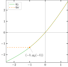
Figure 1: The rate functions and pressures of Theorems  ‣ 1.1 and A for some Bernoulli measures ${\mathbb{P}}$ and ${\mathbb{Q}}$; see Section 2.1. The rate functions are infinite wherever not drawn.

The next two theorems involve only one measure ${\mathbb{P}}$. We remark that the pair $({\mathbb{P}},{\mathbb{P}})$ is admissible if and only if ${\mathbb{P}}$ satisfies both 1.1 and 1.1. As a consequence, the conclusions of Theorem  ‣ 1.1 hold under the assumptions of Theorems B and C; in particular $I_{{\mathbb{P}}}$ and $q_{{\mathbb{P}}}$ are well defined, and the numbers $\gamma_{+}\in(-\infty,0]$ and $\gamma_{-}\in[-\infty,0]$ defined in (1.12) are actual limits.

Theorem B (LDP for $\frac{1}{n}\ln V_{n}$).

If ${\mathbb{P}}\in{\cal P}_{\textnormal{inv}}(\Omega)$ satisfies 1.1 and 1.1, then the following hold:

1. The sequence $(\tfrac{1}{n}\ln V_{n})_{n\in{\mathbb{N}}}$ is exponentially tight and satisfies the LDP with respect to ${\mathbb{P}}$ with the good, convex rate function $I_{V}$ given by

   $$I_{V}(s):=\begin{cases}\infty&\text{if }s<0,\\ \inf_{r\geq s}(r-s+I_{{\mathbb{P}}}(r))&\text{if }s\geq 0.\end{cases}$$ (1.22)

2. For all $\alpha\in{\mathbb{R}}$, the limit in (1.5) exists in $(0,\infty]$,

   $$q_{V}(\alpha)=\max\{q_{{\mathbb{P}}}(\alpha),q_{{\mathbb{P}}}(-1)\},$$ (1.23)

   and the Legendre–Fenchel duality relations $q_{V}=I_{V}^{*}$ and $I_{V}=q_{V}^{*}$ hold. Moreover,

   $$I_{V}(0)=-q_{{\mathbb{P}}}(-1)\geq-\gamma_{+}.$$ (1.24)

Remark 1.10.

The rate function $I_{V}$ corresponds to $I_{W}$ in the special case ${\mathbb{Q}}={\mathbb{P}}$. While one can, of course, choose ${\mathbb{Q}}={\mathbb{P}}$ in Theorem A (in this case it suffices that ${\mathbb{P}}$ satisfies 1.1 and 1.1), this special case is not equivalent to Theorem B. Indeed, $W_{n}$ and $V_{n}$ are still distinct in their definition and underlying probability space. It is known that the range of applicability of almost sure entropy estimation via $W_{n}$ is strictly smaller than that via $V_{n}$ (or $R_{n}$); see [OW93] and [Shi93, §4].

Theorem C (LDP for $\frac{1}{n}\ln R_{n}$).

If ${\mathbb{P}}\in{\cal P}_{\textnormal{inv}}(\Omega)$ satisfies 1.1, 1.1 and 1.4, then the following hold:

1. The sequence $(\tfrac{1}{n}\ln R_{n})_{n\in{\mathbb{N}}}$ is exponentially tight and satisfies the LDP with respect to ${\mathbb{P}}$ with the good (possibly nonconvex) rate function $I_{R}$ given by

   $$I_{R}(s):=\begin{cases}\infty&\text{if }s<0,\\ -\gamma_{+}&\text{if }s=0,\\ \inf_{r\geq s}(r-s+I_{{\mathbb{P}}}(r))&\text{if }s>0.\end{cases}$$ (1.25)

2. For all $\alpha\in{\mathbb{R}}$, the limit in (1.4) exists in $(0,\infty]$ and

   $$q_{R}(\alpha)=\max\{q_{{\mathbb{P}}}(\alpha),\gamma_{+}\}.$$ (1.26)

   Moreover, $q_{R}=I_{R}^{*}$.

3. We have the following relations: $I_{R}$ is convex $\iff$ $I_{R}=I_{V}$ $\iff$ $q_{R}=q_{V}$ $\iff$ $\gamma_{+}=q_{{\mathbb{P}}}(-1)$ $\iff$ $I_{{\mathbb{P}}}(-\gamma_{+})=0$ $\iff$ $q_{{\mathbb{P}}}(\alpha)=-\gamma_{+}\alpha$ for all $\alpha\leq 0$ $\impliedby$ $\gamma_{+}=\gamma_{-}$ $\iff$ $I_{{\mathbb{P}}}(s)=\infty$ for all $s\neq-\gamma_{+}$$\iff$ $h({\mathbb{P}})=h_{\textnormal{top}}(\operatorname{supp}{\mathbb{P}})$. Moreover, if $\tau_{n}=O(1)$ and $C_{n}=O(1)$, then all the above properties are actually equivalent.

By their definition, the rate functions $I_{R}$ and $I_{V}$ may differ only at $0$, and by (1.24) we have $I_{R}(0)=-\gamma_{+}\leq I_{V}(0)$; see Figure 2 for an illustration. Part iii gives many technical conditions equivalent to $I_{R}=I_{V}$, the most notable of which is the convexity of $I_{R}$. The situation where $I_{R}=I_{V}$ should be seen as quite degenerate; in the generic case, we have $I_{R}(0)<I_{V}(0)$, as strikingly illustrated by the examples in Sections 2.1 and 2.2. The generic inequality $I_{R}(0)<I_{V}(0)$ is due to fact that the definition of $R_{n}$ allows for some overlaps (characterized by $R_{n}<n$) which are excluded in $V_{n}$. These overlaps, which make the LDP for $(\frac{1}{n}\ln R_{n})_{n\in{\mathbb{N}}}$ highly interesting, were widely studied in other contexts; see the discussion and references in Section 1.3. With help of 1.4, we will show in Section 4.2 that ${\mathbb{P}}\{x:R_{n}(x)<n\}$ asymptotically decreases like $\mathrm{e}^{n\gamma_{+}}$, which explains the equality $I_{R}(0)=-\gamma_{+}$.

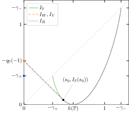
Figure 2: The rate functions and pressures of Theorems  ‣ 1.1 and A–C for some Bernoulli measure ${\mathbb{P}}$; see Section 2.1. The rate functions are infinite wherever not drawn.

Remark 1.11.

If $\gamma_{+}=0$, then $I_{{\mathbb{P}}}(0)=0$ by (1.15), and thus $q_{{\mathbb{P}}}(\alpha)=I_{{\mathbb{P}}}^{*}(\alpha)=0$ for all $\alpha\leq 0$. In this case, we easily see that $I_{V}=I_{R}=I_{{\mathbb{P}}}$ and $q_{V}=q_{R}=q_{{\mathbb{P}}}$.

Remark 1.12.

The relation (1.26) can be written as

$$q_{R}(\alpha)=\begin{cases}\gamma_{+}&\text{if }\alpha<\alpha_{*},\\ q_{{\mathbb{P}}}(\alpha)&\text{if }\alpha\geq\alpha_{*},\end{cases}$$ (1.27)

where $\alpha_{*}\leq 0$ is such that $q_{{\mathbb{P}}}(\alpha_{*})=\gamma_{+}$. If $\gamma_{+}=0$, then we can take any $\alpha_{*}\leq 0$ in view of Remark 1.11. If $\gamma_{+}<0$, then $q_{{\mathbb{P}}}(-1)\leq\gamma_{+}<0=q_{{\mathbb{P}}}(0)$ by (1.24), so the point $\alpha_{*}$ is unique and satisfies $\alpha_{*}\in[-1,0)$, with $\alpha_{*}=-1$ if and only if $I_{V}=I_{R}$.

1.3 Outline of the proof for a toy model

We present a natural toy model, consisting of a mixture of geometric distributions, which not only provides the correct rate functions for $W_{n}$ and $V_{n}$, but also illustrates the method of our proof. We then modify the toy model in order to take overlaps (corresponding to $R_{n}<n$) into account and guess the correct rate function for $R_{n}$.

Approximations of waiting times and return times by geometric random variables (or exponential random variables in the scaling limit) have been widely studied, typically under mixing assumptions; see e.g. [GS97, CGS99, HSV99, AG01, HV10] and [AdAG21] for a recent overview and more exhaustive references. As often emphasized in the literature, possible overlaps, which are tightly related to Poincaré recurrence times (see [AV08, AC15, AdAG21]), play a crucial role in such approximations. We shall further comment on Poincaré recurrence times at the end of Section 4.2.

Our decoupling assumptions do not seem to imply any of the very sharp exponential approximations that are available in the literature. In comparison, the geometric approximation that we prove in Section 3.1 are quite loose in the sense that scaling factors and error terms may grow subexponentially. Yet, it suffices to establish the LDPs of interest.

Geometric approximation.

We start with the following interpretation of $W_{n}(x,y)$: first $x$ is drawn at random according to the law ${\mathbb{P}}$ and $y$ is drawn at random according to the law ${\mathbb{Q}}$, independently of $x$. Then, for each $k\in{\mathbb{N}}$, we check whether $y_{k}^{k+n-1}=x_{1}^{n}$ or not. Once $x_{1}^{n}$ is given, shift invariance implies that ${\mathbb{Q}}\{y\in\Omega:y_{k}^{k+n-1}=x_{1}^{n}\}={\mathbb{Q}}_{n}(x_{1}^{n})$ for each $k\in{\mathbb{N}}$, and we can view $W_{n}$ as the time of the first “success” in a series of attempts (indexed by $k$). If the attempts were mutually independent, $W_{n}$ would be a geometric random variable with random parameter $p_{n}={\mathbb{Q}}_{n}(x_{1}^{n})$. Of course, these attempts are not independent: even if ${\mathbb{Q}}$ is a Bernoulli measure, the attempts $k$ and $k^{\prime}$ are only independent for $|k^{\prime}-k|\geq n$. However, it turns out, due to our decoupling assumptions, that the asymptotic behavior of $W_{n}$ at the scale that is relevant to our LDP is accurately captured by this simplified geometric model.

We now define the toy model properly. Let $\widetilde{W}_{n}$ the random variable whose law $\nu_{n}$ on ${\mathbb{N}}$ is given by

$$\nu_{n}(k):=\sum_{u\in{\cal A}^{n}}{\mathbb{P}}_{n}(u){\mathbb{Q}}_{n}(u)(1-{\mathbb{Q}}_{n}(u))^{k-1},$$ (1.28)

for every $k\in{\mathbb{N}}$. This is a simple mixture of geometric distributions, motivated by the above discussion. The next proposition describes the large deviations of $\widetilde{W}_{n}$. Since it is introduced only for illustration purposes, and since the actual proof of the proposition relies on estimates which are similar to — but simpler than — those we provide for $W_{n}$ in the main body of the paper, we limit ourselves to sketching the proof. The interested reader will easily be able to fill in the details.

Proposition 1.13.

If the pair $({\mathbb{P}},{\mathbb{Q}})$ is admissible, then the sequence $(\frac{1}{n}\ln\widetilde{W}_{n})_{n\in{\mathbb{N}}}$ satisfies the LDP with the rate function $I_{W}$ defined in (1.19).

Sketch of the proof..

For each $s\in M_{n}:=\{\frac{1}{n}\ln k:k\in{\mathbb{N}}\}$, the probability that $\frac{1}{n}\ln\widetilde{W}_{n}$ equals $s$ is given by

$$\nu_{n}(\mathrm{e}^{ns})=\sum_{u\in{\cal A}^{n}}{\mathbb{P}}_{n}(u){\mathbb{Q}}_{n}(u)(1-{\mathbb{Q}}_{n}(u))^{\mathrm{e}^{ns}-1}=\int_{(0,\infty)}\mathrm{e}^{-rn}(1-\mathrm{e}^{-rn})^{\mathrm{e}^{ns}-1}\mathop{\mathrm{\mathstrut d}}\nolimits\!\mu_{n}(r),$$ (1.29)

where we denote by $\mu_{n}$ the distribution of $-\frac{1}{n}\ln{\mathbb{Q}}_{n}$ with respect to ${\mathbb{P}}$. Now using that $\mathrm{e}^{-rn}$ is very small for $n$ large, a formal first order Taylor expansion yields

$$(1-\mathrm{e}^{-rn})^{\mathrm{e}^{ns}-1} =\exp((\mathrm{e}^{ns}-1)\ln(1-\mathrm{e}^{-rn}))\sim\exp(-(\mathrm{e}^{ns}-1)\mathrm{e}^{-rn})\sim\exp(-\mathrm{e}^{n(s-r)}).$$ (1.30)

We thus have a cut-off phenomenon: the above vanishes superexponentially when $r<s$, and is very close to $1$ when $r>s$. Formal substitution into (1.29) yields

$$\nu_{n}(\mathrm{e}^{ns})\sim\int_{(s,\infty)}\mathrm{e}^{-rn}\mathop{\mathrm{\mathstrut d}}\nolimits\!\mu_{n}(r).$$

We remark that this cut-off argument corresponds to retaining, in the sum in (1.28), only the $u\in{\cal A}^{n}$ such that ${\mathbb{Q}}_{n}(u)\lesssim\mathrm{e}^{-ns}$.

Now, for $s>0$ and $\epsilon$ small, the set $B(s,\epsilon)\cap M_{n}$ contains approximately $\mathrm{e}^{n(s+\epsilon)}-\mathrm{e}^{n(s-\epsilon)}\sim\mathrm{e}^{sn}$ points, so

$$\nu_{n}\left\{k\in{\mathbb{N}}:\frac{1}{n}\ln k\in B(s,\epsilon)\right\}\sim\mathrm{e}^{sn}\nu_{n}(\mathrm{e}^{ns})\sim\int_{(s,\infty)}\mathrm{e}^{(s-r)n}\mathop{\mathrm{\mathstrut d}}\nolimits\!\mu_{n}(r).$$ (1.31)

Formally, Theorem  ‣ 1.1 says that $\mathop{\mathrm{\mathstrut d}}\nolimits\!\mu_{n}(r)\sim\mathrm{e}^{-nI_{{\mathbb{Q}}}(r)}\mathop{\mathrm{\mathstrut d}}\nolimits\!r$, and a saddle-point approximation in (1.31) then yields

$$\frac{1}{n}\ln\nu_{n}\left\{k\in{\mathbb{N}}:\frac{1}{n}\ln k\in B(s,\epsilon)\right\}\sim\sup_{r\geq s}(s-r-I_{{\mathbb{Q}}}(r))=-I_{W}(s).$$

The same conclusion applies to the case $s=0$ without the need for any cut-off argument. This local formulation of the LDP (i.e. concerning only small balls) implies the weak LDP (see Section 4), which can in turn be promoted to a full LDP using the arguments of Section 5. ∎

The fact that we consider $W_{n}(x,y)$ for $x$ and $y$ that are mutually independent was an important ingredient of the above argument. When moving on to $V_{n}$ and $R_{n}$ (and replacing ${\mathbb{Q}}$ with ${\mathbb{P}}$), we look for occurrences of $x_{1}^{n}$, not in an independent sample $y$, but in $x$ itself, which introduces more dependence. Conditioned on the event $[u]$ for some $u\in{\cal A}^{n}$, the random variable $V_{n}$ corresponds to the first success time of a series of attempts, where the $k$-th attempt is successful if $x_{n+k}^{2n+k-1}=u$. Contrary to the case of $W_{n}$, the conditional success probability given $[u]$ of the $k$-th attempt is not simply given by ${\mathbb{P}}_{n}(u)$ since the coordinates $x_{1}^{n}$ and $x_{n+k}^{2n+k-1}$ are not independent in general. However, by our decoupling assumptions, and since the intervals $[1,n]$ and $[n+k,2k+k-1]$ do not overlap, this added dependence will not actually alter the asymptotics. The arguments of Proposition 1.13 then suggest that $V_{n}$ obeys the LDP with the rate function $I_{V}$ of (1.22).

Return time and overlaps.

The picture for $R_{n}$ is more complicated: while the dependence between $x_{k+1}^{k+n}$ and $x_{1}^{n}$ will not significantly alter our estimates for $k$ very large, this dependence will play a major role when $k<n$, due to overlap; see the examples in Section 2. We shall prove in Section 4.2 that, under the assumptions of Theorem C,

$$\lim_{n\to\infty}\frac{1}{n}\ln{\mathbb{P}}\{x:R_{n}(x)<n\}=\gamma_{+}.$$ (1.32)

This suggests the following picture: with probability close to $\mathrm{e}^{n\gamma_{+}}$ we have “very quick return” ($R_{n}<n$), and with probability close to $1-\mathrm{e}^{n\gamma_{+}}$ we start a series of trials as in the case of $V_{n}$. As before, let us pretend these trials are independent, and that their probability of success is exactly ${\mathbb{P}}_{n}(x_{1}^{n})$. Noting that the asymptotics of $\frac{1}{n}\ln R_{n}$ is not affected by adding to $R_{n}$ quantities of order $n$, we are led to introduce a toy model $\widetilde{R}_{n}$ for $R_{n}$ whose law $\rho_{n}$ on ${\mathbb{N}}$ is given by

$$\rho_{n}(k):=\mathrm{e}^{n\gamma_{+}}\delta_{k,1}+(1-\mathrm{e}^{n\gamma_{+}})\nu_{n}(k)$$ (1.33)

for every $k\in{\mathbb{N}}$, where $\nu_{n}$ is as in (1.28) with ${\mathbb{Q}}={\mathbb{P}}$. A straightforward adaptation of Proposition 1.13, taking the first term in (1.33) into account at $s=0$, and also using that $\gamma_{+}\geq\sup_{r\geq 0}(-r-I_{{\mathbb{P}}}(r))$ by Theorem  ‣ 1.1.iii.a., shows that $\widetilde{R}_{n}$ satisfies the LDP with the rate function $I_{R}$ of (1.25).

Turning the sketch into a proof.

We now briefly comment on how the above sketch will be made rigorous in the main body of the paper. In Section 3.1, we establish that for fixed $x$, the random variable $W_{n}(x,\cdot\,)$ on $(\Omega,{\mathbb{Q}})$ is indeed approximated by a geometric random variable at the exponential scale. The above cut-off argument is made rigorous in Proposition 3.5. The corresponding estimates for $R_{n}$ and $V_{n}$ are presented in Section 3.2.

The saddle-point approximation mentioned above is made rigorous by the variation of Varadhan’s lemma provided in Lemma 4.1, which then leads to the weak LDP for the sequences of interest. As with the above toy model, we need to treat the cases $s>0$ (Section 4.1) and $s=0$ (Section 4.2) separately — the latter is particularly subtle for $R_{n}$ and 1.4 will be needed to establish (1.32). With the weak LDPs at hand, the main results are proved in Section 5.

2 Examples

Decoupling assumptions are satisfied by many important classes of examples, and have allowed to simplify and unify the proofs of various large deviation principles that existed in many, sometimes rather technical, forms in the literature. The range of applicability of 1.1 and 1.1 has already been discussed in [CJPS19, BCJP21, CDEJR22, CDEJR23].

We describe in this section some classes of examples that serve as illustrations of different features of our main results. Sections 2.1–2.5 each assume some level of familiarity with the specific examples on the readers’ part, and may be skipped entirely without affecting the reader’s ability to understand the proofs of the main theorems. We now briefly summarize the role of each of these examples.

1. In the Bernoulli (IID) case (Section 2.1), formulae for the different pressures and rate functions can be quickly derived, and are easy to understand. To the best of our knowledge, the global aspect of the LDPs in Theorems A–C as well as the ability to consider distinct measures ${\mathbb{P}}$ and ${\mathbb{Q}}$ in Theorem A are new even in this most basic class of examples.

2. By going from Bernoulli measures to Markov measures (Section 2.2), we start seeing the benefit of allowing the length $\ell$ of $\xi$ in 1.1 to satisfy $0\leq\ell\leq\tau_{n}$ instead of requiring $\ell=\tau_{n}$. Markov measures also make the role of periodicity in 1.4 very clear.

3. Discussing our assumptions and results in the setup of equilibrium measures of potentials enjoying Bowen’s regularity condition (Section 2.3) allows us to compare our results to existing ones, most notably to those of [AdACG22] where the pressures $q_{W}$ and $q_{R}$ were studied.

4. We then discuss two situations in which Bowen’s regularity condition can be lifted. While carrying distinct history and intuition, they both reveal the same two aspects of our decoupling assumptions. First, they make a case that allowing a certain amount of growth for the sequence $(C_{n})_{n\in{\mathbb{N}}}$ in 1.1 and 1.1 is beneficial. Second, they show that our assumptions apply in phase-transition situations, and in particular do not imply ergodicity. These generalizations are:

   1. equilibrium measures for summable interactions in statistical mechanics (Section 2.4.1);

   2. equilibrium measures for $g$-functions, i.e. $g$-measures (Section 2.4.2).

   While our results do not seem to apply to the class of weak Gibbs measures in full generality (see Section 2.4), the measures discussed in Sections 2.4.1 and 2.4.2 are weak Gibbs.

5. Finally, the so-called class of hidden Markov models (Section 2.5) shows our assumptions apply to measures which are far from Gibbsian. Hidden Markov models also provide examples of pairs of measures $({\mathbb{P}},{\mathbb{Q}})$ where the distributions of $(\frac{1}{n}\ln W_{n})_{n\in{\mathbb{N}}}$ lack exponential tightness, showing that $I_{W}$ (see Theorem A) need not be a good rate function when ${\mathbb{Q}}\neq{\mathbb{P}}$. To the authors’ knowledge, even the conclusions of Theorem  ‣ 1.1 in this setup are new.

As abundantly discussed in [BJPP18, CJPS19, BCJP21, CDEJR22, CDEJR23], repeated quantum measurement processes give rise to a very rich class of measures satisfying our decoupling assumptions, yet displaying remarkable singularities — some being, once again, far from Gibbsian. For reasons of space, we do not repeat such a discussion in the present paper.

2.1 Bernoulli measures

Consider the simple case ${\mathbb{P}}={\mathbb{P}}_{1}^{\otimes{\mathbb{N}}}$ and ${\mathbb{Q}}={\mathbb{Q}}_{1}^{\otimes{\mathbb{N}}}$, where ${\mathbb{P}}_{1}$ and ${\mathbb{Q}}_{1}$ are measures on ${\cal A}$, with ${\mathbb{P}}_{1}\ll{\mathbb{Q}}_{1}$. 1.1, 1.1 and 1.4 obviously hold with $C_{n}=1$ and $\tau_{n}=0$ for all $n$. Note that, as a random variable on $(\Omega,{\mathbb{P}})$, the map $x\mapsto-\tfrac{1}{n}\ln{\mathbb{Q}}_{n}(x_{1}^{n})=\frac{1}{n}\sum_{i=1}^{n}(-\ln{\mathbb{Q}}_{1}(x_{i}))$ is simply the average of IID random variables supported on the finite set $\{-\ln{\mathbb{Q}}_{1}(a):a\in\operatorname{supp}{\mathbb{P}}_{1}\}\subset{\mathbb{R}}$. By independence, $q_{{\mathbb{Q}}}(\alpha)$ is easily seen to coincide with the cumulant-generating function:

$$q_{{\mathbb{Q}}}(\alpha)=\ln\int_{{\cal A}}\mathrm{e}^{-\alpha\ln{\mathbb{Q}}_{1}(a)}\mathop{\mathrm{\mathstrut d}}\nolimits\!{\mathbb{P}}_{1}(a)=\ln\sum_{a\in\operatorname{supp}{\mathbb{P}}_{1}}{\mathbb{P}}_{1}(a){\mathbb{Q}}_{1}(a)^{-\alpha}.$$ (2.1)

The LDP proved in Theorem  ‣ 1.1 then follows from standard results. We mention two methods which lead to different expressions of the rate function $I_{{\mathbb{Q}}}$.

Method 1. Since $\ln{\mathbb{Q}}_{n}(x_{1}^{n})$ is a sum of IID random variables, Cramér’s theorem [DZ09, §2.2.1] yields the stated LDP with a rate function given by the Legendre–Fenchel transform of the cumulant-generating function (2.1), i.e. with a rate function $I_{{\mathbb{Q}}}=q_{{\mathbb{Q}}}^{*}$. This can be seen as a special case of the Gärtner–Ellis theorem [DZ09, §2.3], which applies here since by (2.1) the function $q_{{\mathbb{Q}}}$ is differentiable (and actually real-analytic).

Method 2. One can instead appeal to a combination of Sanov’s theorem and the contraction principle [DZ09, §2.1.1–2.1.2] to obtain the LDP with rate function

$$I_{{\mathbb{Q}}}(s)=\inf_{\mu\in L_{s}}H_{\mathrm{r}}(\mu|{\mathbb{P}}_{1}),$$ (2.2)

where $H_{\mathrm{r}}$ denotes the relative entropy and $L_{s}$ is the set of probability measures $\mu\ll{\mathbb{P}}_{1}$ (hence also satisfying $\mu\ll{\mathbb{Q}}_{1}$) on ${\cal A}$ subject to the constraint

$$-\sum_{a\in{\cal A}}\mu(a)\ln{\mathbb{Q}}_{1}(a)=s.$$ (2.3)

When $s\notin[-\ln\max_{a\in{\cal A}}{\mathbb{Q}}_{1}(a),-\ln\min_{a\in\operatorname{supp}{\mathbb{Q}}_{1}}{\mathbb{Q}}_{1}(a)]$, the set $L_{s}$ is empty and the infimum is set to $\infty$ by convention. Note that $I_{{\mathbb{Q}}}$ vanishes at the unique point $s=-\sum_{a\in{\cal A}}{\mathbb{P}}_{1}(a)\ln{\mathbb{Q}}_{1}(a)=h_{\textnormal{c}}({\mathbb{P}}|{\mathbb{Q}})$, where the infimum in (2.2) is attained at $\mu={\mathbb{P}}_{1}$.

We now turn to Theorems B and C, and we discuss in particular the convexity of $I_{R}$. The relevant quantities are easily expressed in terms of ${\mathbb{P}}_{1}$:

$$\gamma_{+} =\ln\max_{a\in\operatorname{supp}{\mathbb{P}}_{1}}{\mathbb{P}}_{1}(a), h_{\textnormal{top}}(\operatorname{supp}{\mathbb{P}}) =\ln|\operatorname{supp}{\mathbb{P}}_{1}|,$$

$$\gamma_{-} =\ln\min_{a\in\operatorname{supp}{\mathbb{P}}_{1}}{\mathbb{P}}_{1}(a), q_{{\mathbb{P}}}(-1) =\ln\sum_{a\in\operatorname{supp}{\mathbb{P}}_{1}}{\mathbb{P}}_{1}(a)^{2}.$$

In view of these expressions, $\gamma_{-}\leq q_{{\mathbb{P}}}(-1)\leq\gamma_{+}$ with strict inequalities unless ${\mathbb{P}}_{1}$ is constant on its support. To see this, notice that $\sum_{a\in{\cal A}}{\mathbb{P}}_{1}(a)^{2}$ is the expectation of the function $a\mapsto{\mathbb{P}}_{1}(a)$ with respect to the measure ${\mathbb{P}}_{1}$ on ${\cal A}$. To discuss the convexity of $I_{R}$ we distinguish two cases.

Singular case. If ${\mathbb{P}}_{1}$ is constant on its support, then $\gamma_{-}=q_{{\mathbb{P}}}(-1)=\gamma_{+}$, so $I_{R}$ is convex by Theorem C.iii. Moreover, we readily obtain $h({\mathbb{P}})=h_{\textnormal{top}}(\operatorname{supp}{\mathbb{P}}),$ so ${\mathbb{P}}$ is indeed the measure of maximal entropy on its support, in accordance with Theorem C.iii. Next, since $-\frac{1}{n}\ln{\mathbb{P}}_{n}(x_{1}^{n})=h({\mathbb{P}})$ almost surely, the rate function $I_{{\mathbb{P}}}$ vanishes at $h({\mathbb{P}})$ and is infinite everywhere else. Dual to this, $q_{{\mathbb{P}}}(\alpha)=h({\mathbb{P}})\alpha$ for all $\alpha\in{\mathbb{R}}$. In the quite extreme case where $|\operatorname{supp}{\mathbb{P}}_{1}|=1$, i.e. if ${\mathbb{P}}$ is a Dirac measure on an orbit of period 1, we find $h({\mathbb{P}})=0$ and $q_{{\mathbb{P}}}(\alpha)=0$ for all $\alpha\in{\mathbb{R}}$.

Generic case. If ${\mathbb{P}}_{1}$ is not constant on its support, then $\gamma_{-}<q_{{\mathbb{P}}}(-1)<\gamma_{+}$, and thus the rate function $I_{R}$ is nonconvex by Theorem C.iii. In the present setup, it is easy to understand why $I_{R}(0)<I_{V}(0)$, as we now discuss. Let $\epsilon$ be small and $n$ be large. On the one hand, if $\hat{a}\in{\cal A}$ is such that $\ln{\mathbb{P}}_{1}(\hat{a})=\gamma_{+}$, we find $R_{n}(x)=1$ for all $x\in[\hat{a}^{n+1}]$, so

$${\mathbb{P}}\{x:R_{n}(x)\leq\mathrm{e}^{\epsilon n}\}\geq{\mathbb{P}}\left\{x:R_{n}(x)=1\right\}\geq{\mathbb{P}}_{n+1}(\hat{a}^{n+1})=\exp\left((n+1)\gamma_{+}\right).$$ (2.4)

On the other hand, $V_{n}(x)=k$ implies that $x\in[u]\cap T^{-n-k+1}[u]$ for some $u\in{\cal A}^{n}$, so

$${\mathbb{P}}\{x:V_{n}(x)=k\} \leq\sum_{u\in{\cal A}^{n}}{\mathbb{P}}([u]\cap T^{-n-k+1}[u])=\sum_{u\in{\cal A}^{n}}{\mathbb{P}}_{n}(u)^{2}$$

$$=\Big{(}\sum_{a\in{\cal A}}{\mathbb{P}}_{1}(a)^{2}\Big{)}^{n}=\exp\left(nq_{{\mathbb{P}}}(-1)\right),$$

where we have used (2.1) with ${\mathbb{Q}}={\mathbb{P}}$. Thus,

$${\mathbb{P}}\{x:V_{n}(x)\leq\mathrm{e}^{\epsilon n}\}\leq\sum_{k=1}^{\lfloor\mathrm{e}^{\epsilon n}\rfloor}{\mathbb{P}}\{x:V_{n}(x)=k\}\leq\exp\left(n\epsilon+nq_{{\mathbb{P}}}(-1)\right).$$ (2.5)

Therefore, for $\epsilon$ small enough, the right-hand side of (2.4) decays exponentially faster than the right-hand side of (2.5) since $q_{{\mathbb{P}}}(-1)<\gamma_{+}$ in the generic case. The estimates (2.4) and (2.5), despite the rather crude inequalities in (2.4), turn out to be sharp at the exponential scale. Indeed, we find $I_{V}(0)=-q_{{\mathbb{P}}}(-1)$ and $I_{R}(0)=-\gamma_{+}$ in Theorems B and C.

Remark 2.1.

For Bernoulli measures, in the case ${\mathbb{Q}}={\mathbb{P}}$, $W_{n}$ and $V_{n}$ have the same law.

We provide three figures corresponding to Bernoulli measures, the first two of which were displayed in Section 1.2:

• Figure 1: ${\cal A}=\{\textsf{0},\textsf{1},\textsf{2}\}$ and ${\mathbb{P}}_{1}=0.2\,\delta_{\textsf{0}}+0.3\,\delta_{\textsf{1}}+0.5\,\delta_{\textsf{2}}$ and ${\mathbb{Q}}_{1}=0.6\,\delta_{\textsf{0}}+0.3\,\delta_{\textsf{1}}+0.1\,\delta_{\textsf{2}}$.

• Figure 2: ${\cal A}=\{\textsf{0},\textsf{1}\}$ and ${\mathbb{P}}_{1}={\mathbb{Q}}_{1}=0.3\,\delta_{\textsf{0}}+0.7\,\delta_{\textsf{1}}$.

• Figure 3: ${\cal A}=\{\textsf{0},\textsf{1},\textsf{2}\}$ and ${\mathbb{P}}_{1}={\mathbb{Q}}_{1}=0.15\,\delta_{\textsf{0}}+0.15\,\delta_{\textsf{1}}+0.7\,\delta_{\textsf{2}}$. Notice that $\ln{\mathbb{P}}_{1}(\textsf{0})=\ln{\mathbb{P}}_{1}(\textsf{1})=-\gamma_{-}$. Such degeneracy implies that the second term in (1.17) takes the value $\ln 2$ for $s=-\gamma_{-}$. Indeed, when $\epsilon$ is very small, the cardinality in (1.17) is essentially $2^{n}$. As a consequence, $I_{{\mathbb{P}}}(-\gamma_{-})=-\gamma_{-}-\ln 2$. A similar phenomenon occurs at $-\gamma_{+}$ if several letters in ${\cal A}$ have maximum probability.

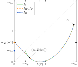
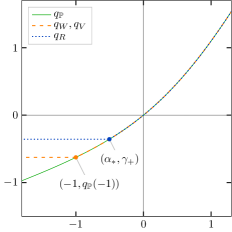
Figure 3: Rate functions and pressures for a Bernoulli measure with degenerate least probable letter. The coordinates of the point $A$ are $(-\gamma_{-},-\gamma_{-}-\ln 2)$. Rate functions are infinite wherever not drawn.

2.2 Irreducible Markov measures

Let ${\mathbb{P}}$ and ${\mathbb{Q}}$ be two irreducible, stationary Markov measures on ${\cal A}$, with transition matrices $P=[P_{i,j}]_{i,j\in{\cal A}}$ and $Q=[Q_{i,j}]_{i,j\in{\cal A}}$ respectively. Then,

$${\mathbb{P}}_{n}(x_{1}^{n})={\mathbb{P}}_{1}(x_{1})\prod_{k=1}^{n-1}P_{x_{k},x_{k+1}},\qquad{\mathbb{Q}}_{n}(x_{1}^{n})={\mathbb{Q}}_{1}(x_{1})\prod_{k=1}^{n-1}Q_{x_{k},x_{k+1}},$$ (2.6)

where ${\mathbb{P}}_{1}$ and ${\mathbb{Q}}_{1}$ are the (unique and fully supported) invariant probability vectors for the matrices $P$ and $Q$ respectively. We assume, furthermore, that $Q_{i,j}=0$ implies $P_{i,j}=0$, which ensures that ${\mathbb{P}}_{n}\ll{\mathbb{Q}}_{n}$ for all $n\in{\mathbb{N}}$. It follows from Lemma A.3 in [CJPS19] that 1.1 and 1.1 hold with $C_{n}=O(1)$ and $\tau_{n}=O(1)$, so the pair $({\mathbb{P}},{\mathbb{Q}})$ is admissible. Similar arguments also yield 1.4. It is worth noting that if $P$ is further assumed to be aperiodic, then we can take some fixed $\ell$ in (1.10), whereas if $P$ is merely irreducible, then $\ell$ must be allowed depend on $u$ and $v$. This illustrates the importance of the condition $\ell\leq\tau_{n}$ in 1.1 instead of $\ell=\tau_{n}$; see the discussion in [CJPS19, §§2.5;A.1].

Our results thus apply to the setup described here. As in the previous example, the conclusions of Theorem  ‣ 1.1 can be derived using classical methods, which yield natural expressions for $I_{{\mathbb{Q}}}$ and $q_{{\mathbb{Q}}}$, as we now show.

Method 1. In view of (2.6), the pressure is easily seen to be given by

$$q_{{\mathbb{Q}}}(\alpha)=\ln\operatorname{spr}(M(\alpha)),$$

where the spectral radius is computed for the deformation of the stochastic matrix $P$ defined by $M_{i,j}(\alpha):=P_{i,j}Q_{i,j}^{-\alpha}$. By the Perron–Frobenius theorem and analytic perturbation theory, $\alpha\mapsto q_{{\mathbb{Q}}}(\alpha)$ is real-analytic, so the LDP for $(-\frac{1}{n}\ln{\mathbb{Q}}_{n})_{n\in{\mathbb{N}}}$ with the rate function $I_{{\mathbb{Q}}}=q_{{\mathbb{Q}}}^{*}$ follows from the Gärtner–Ellis theorem [DZ09, §2.3].

Method 2. From (2.6), we see that

$$\ln{\mathbb{Q}}_{n}(x_{1}^{n})=\sum_{k=1}^{n-1}\ln Q_{x_{k},x_{k+1}}+O(1)$$

for all $x\in\operatorname{supp}{\mathbb{P}}\subseteq\operatorname{supp}{\mathbb{Q}}$, so the LDP for $(-\frac{1}{n}\ln{\mathbb{Q}}_{n})_{n\in{\mathbb{N}}}$ reduces to that of a sequence of Birkhoff sums. By Sanov’s theorem applied the pair empirical measures ${\cal E}_{n}(x):=\frac{1}{n}\sum_{k=1}^{n}\delta_{(x_{k},x_{k+1})}\in{\cal P}({\cal A}^{2})$ and the contraction principle, one derives the expression

$$I_{{\mathbb{Q}}}(s)=\inf_{\mu\in L_{s}^{(2)}}H_{\mathrm{r}}(\mu|\mu_{1}\otimes P),$$ (2.7)

where $L_{s}^{(2)}$ is the set of probability measures $\mu$ on ${\cal A}\times{\cal A}$ such that $\mu\ll\mu_{1}\otimes P$, $\mu_{1}=\mu_{2}$, and

$$\sum_{i,j\in{\cal A}}\mu(i,j)\ln Q_{i,j}=-s;$$

see [DZ09, §3.1.3] or Lemma 4.49 in [DS89]. Here, $\mu_{1}$ denotes the first marginal of $\mu$, and $\mu_{1}\otimes P$ denotes the measure on ${\cal A}\times{\cal A}$ defined by $(\mu_{1}\otimes P)(i,j)=\mu_{1}(i)P_{i,j}$. Note that $I_{{\mathbb{Q}}}$ vanishes at the single point $s=-\sum_{i,j\in{\cal A}}{\mathbb{P}}_{2}(i,j)\ln Q_{i,j}=h_{\textnormal{c}}({\mathbb{P}}|{\mathbb{Q}})$, where the infimum in (2.7) is attained at $\mu={\mathbb{P}}_{2}$.

We now discuss $I_{R}$ and its convexity, with ${\mathbb{P}}={\mathbb{Q}}$ a Markov measure as above. It is well known that

$$\gamma_{+}=\max_{p\leq|{\cal A}|}\max_{u\in{\cal A}^{p}}\frac{1}{p}\ln\prod_{k=1}^{p}P_{u_{k},u_{k+1}},$$ (2.8)

with cyclic identification $u_{p+1}=u_{1}$; see e.g. Remark 1.ii in [Szp93] or [AdACG22, §3.4]. The heuristic interpretation is the following: while in the generic IID case discussed in Section 2.1 the probability ${\mathbb{P}}\{x:R_{n}(x)\leq\mathrm{e}^{\epsilon n}\}$ was, at exponential scale, captured by the subset $\{x:x_{1}^{n+1}=\mathsf{111}\dotsb\mathsf{11}\}$ of the event $\{x:R_{n}(x)=1\}$ for $n$ large and $\epsilon$ small, now ${\mathbb{P}}\{x:R_{n}(x)\leq\mathrm{e}^{\epsilon n}\}$ is essentially accounted for by the subset $\{x:x_{1}^{n+1}=uuu\dotsb uu_{1}^{r}\}$ of the event $\{x:R_{n}(x)=p\}$, for any $p$ and $u$ that saturate (2.8), and $r=n-\lfloor\frac{n}{p}\rfloor p$. In other words, the key scenario for small return times consists of a periodic orbit repeating some optimal cycle.

By the last part of Theorem C, the function $I_{R}$ is convex if and only if ${\mathbb{P}}$ is the measure of maximal entropy on $\operatorname{supp}{\mathbb{P}}$, that is if and only if ${\mathbb{P}}$ is the Parry measure of $\operatorname{supp}{\mathbb{P}}$, which is characterized by the Perron–Frobenius data of the adjacency matrix of the chain [Par64]; see also [CGS99, §2]. In particular, if $P_{i,j}>0$ for all $i,j\in{\cal A}$, then $I_{R}$ is convex if and only if ${\mathbb{P}}=\pi^{\otimes{\mathbb{N}}}$ with $\pi$ uniform on ${\cal A}$.

Remark 2.2.

One can show that irreducible multi-step Markov measures also satisfy the assumptions in the present paper. In fact, Markov measures and multi-step Markov measures are merely special cases of the equilibrium measures discussed in Section 2.3. For example, in the notation of Section 2.3, one takes $\varphi(x)=\ln P_{x_{1},x_{2}}$ in the case of Markov measures. An explicit computation of $q_{{\mathbb{P}}}$ for a specific Markov chain is provided in [AdACG22].

2.3 Equilibrium measures for Bowen potentials

As mentioned above, our assumptions cover the setups of [CGS99] and [AdACG22], where the large-deviation results are local in the sense that there is some strict subinterval $A\subset{\mathbb{R}}$ such that the large-deviation lower bound and upper bound (see (4.1) and (4.2) below) are only shown to be valid respectively for open sets $O$ contained in $A$ and closed sets $\Gamma$ contained in $A$. The former work considers a single measure ${\mathbb{P}}$ that is the equilibrium measure for a Hölder-continuous potential on a topologically mixing Markov subshift; the latter work, for a potential of summable variations on the full shift.

In particular, Theorem A.i and Theorem C.i prove the following conjecture stated in [AdACG22, §3.3]:

We believe that there exists a non-trivial rate function describing the [global] large deviation asymptotic for both return and waiting times, but this has to be proven using another method.

Moreover, the results of [AdACG22, §3.2] are recovered as special cases of Theorem A.ii and Theorem C.ii. In order to facilitate the translation, we compare notations in Table 1. Note also that what we refer to as pressure is called “$L^{q}$-spectrum” in [AdACG22].

	Pressures			Variable	Important points
Present paper	$q_{{\mathbb{P}}}$	$q_{W}$	$q_{R}$	$\alpha$	$\alpha_{*}$	$\gamma_{+}$	$\gamma_{-}$
[AdACG22]	${\cal M}_{\varphi}$	${\cal W}_{\varphi}$	${\cal R}_{\varphi}$	$q$	$q^{*}_{\varphi}$	$\gamma_{\varphi}^{+}$	$-v_{\varphi}^{+}$

Table 1: A summary of the notational changes between our results and those of [AdACG22].

We first consider the class of Bowen-regular potentials on the full shift, and then discuss the extension to more general subshifts (including those of [CGS99]) in Remark 2.3. We recall that a potential $\varphi$, i.e. a continuous function $\varphi:\Omega\to{\mathbb{R}}$, is called Bowen regular if

$$\sup\left\{\left|\sum_{i=0}^{n-1}\varphi(T^{i}x)-\sum_{i=0}^{n-1}\varphi(T^{i}y)\right|:x\in\Omega,n\in{\mathbb{N}},y\in[x_{1}^{n}]\right\}<\infty,$$ (2.9)

and that this class strictly contains the class of potentials with summable variations, which in turn strictly contains the class of Hölder-continuous potentials; we refer the reader to [Bow74] and [Wal01, §4] for a thorough discussion. We also recall that the topological pressure of any potential $\chi$ is given by

$$p_{\textnormal{top}}(\chi):=\lim_{n\to\infty}\frac{1}{n}\ln\sum_{u\in{\cal A}^{n}}\mathrm{e}^{\sup_{x\in[u]}\sum_{i=0}^{n-1}\chi(T^{i}x)}.$$ (2.10)

Suppose that ${\mathbb{P}}$ and ${\mathbb{Q}}$ are the (necessarily unique [Bow74]) equilibrium measures for the Bowen-regular potentials $\varphi$ and $\psi$ on $\Omega$ in the sense that they belong to ${\cal P}_{\textnormal{inv}}(\Omega)$ and satisfy

$$h({\mathbb{P}})+\int\varphi\mathop{\mathrm{\mathstrut d}}\nolimits\!{\mathbb{P}}=p_{\textnormal{top}}(\varphi)\qquad\text{and}\qquad h({\mathbb{Q}})+\int\psi\mathop{\mathrm{\mathstrut d}}\nolimits\!{\mathbb{Q}}=p_{\textnormal{top}}(\psi),$$ (2.11)

respectively. The measure ${\mathbb{P}}$ then satisfies the Bowen–Gibbs property with respect to $\varphi$, i.e. there exists a constant $K\geq 1$ such that

$$K^{-1}\mathrm{e}^{\sum_{i=0}^{n-1}\varphi(T^{i}x)-np_{\textnormal{top}}(\varphi)}\leq{\mathbb{P}}([x_{1}^{n}])\leq K\mathrm{e}^{\sum_{i=0}^{n-1}\varphi(T^{i}x)-np_{\textnormal{top}}(\varphi)},$$ (2.12)

for every $x\in\Omega$ [Wal01, §4], and one then deduces that it satisfies 1.1 and 1.1 with $\tau_{n}=0$ and $C_{n}=K^{3}$. The same is true for ${\mathbb{Q}}$ with $\psi$, so 1.1 and 1.4 follow from Remarks 1.2 and 1.5 respectively, and thus the pair $({\mathbb{P}},{\mathbb{Q}})$ is admissible. We note that (2.12) is central in the analysis in [AdACG22, §2.1]. In order to simplify some formulae, we assume for the remainder of this subsection that

$$p_{\textnormal{top}}(\varphi)=p_{\textnormal{top}}(\psi)=0,$$ (2.13)

which results in no loss of generality since adding constants to $\varphi$ and $\psi$ does not alter the set of equilibrium measures.

In the setup of the present subsection, the conclusions of Theorem  ‣ 1.1 are well known and can be obtained more directly as follows.

Method 1. The bounds (2.12) imply that

$$q_{{\mathbb{Q}}}(\alpha)=p_{\textnormal{top}}(\varphi-\alpha\psi).$$ (2.14)

In particular, we remark that $q_{{\mathbb{P}}}(-1)=p_{\textnormal{top}}(2\varphi)$; this quantity plays an important role in the formula for $q_{W}$, and is equal to $-I_{W}(0)$. In this setup, $q_{{\mathbb{Q}}}$ is differentiable and, for all $\alpha\in{\mathbb{R}}$,

$$q_{{\mathbb{Q}}}^{\prime}(\alpha)=-\int\psi\mathop{\mathrm{\mathstrut d}}\nolimits\!\mu_{\alpha},$$

where $\mu_{\alpha}$ is the equilibrium measure for the Bowen-regular potential $\varphi-\alpha\psi$; see e.g. Theorems 4.3.3 and 4.3.5 in [Kel98]. The LDP of Theorem  ‣ 1.1 then follows from the Gärtner–Ellis theorem.

Method 2. The same LDP can be obtained from the easy observation that the large deviations of $(-\frac{1}{n}\ln{\mathbb{Q}}_{n})_{n\in{\mathbb{N}}}$ are the same as those of the ergodic averages of $-\psi$ with respect to ${\mathbb{P}}$, which is a well-studied problem; see e.g. [You90, Kif90, Com09, PS17]. The rate function is then given, for all $s\in{\mathbb{R}}$, by

$$I_{{\mathbb{Q}}}(s)=-\sup\left\{\int\varphi\mathop{\mathrm{\mathstrut d}}\nolimits\!\eta+h(\eta):\eta\in{\cal P}_{\textnormal{inv}},\int\psi\mathop{\mathrm{\mathstrut d}}\nolimits\!\eta=-s\right\}.$$ (2.15)

The rate function $I_{{\mathbb{Q}}}$ vanishes at a single point $s=-\int\psi\mathop{\mathrm{\mathstrut d}}\nolimits\!{\mathbb{P}}=h_{\textnormal{c}}({\mathbb{P}}|{\mathbb{Q}})$; the supremum in (2.15) is then reached at $\eta={\mathbb{P}}$.

For all $s\geq 0$, the relations (1.19) and (1.22) give

$$I_{W}(s) =-s-\sup\left\{\int(\varphi+\psi)\mathop{\mathrm{\mathstrut d}}\nolimits\!\eta+h(\eta):\eta\in{\cal P}_{\textnormal{inv}},\int\psi\mathop{\mathrm{\mathstrut d}}\nolimits\!\eta\leq-s\right\},$$

$$I_{V}(s) =-s-\sup\left\{2\int\varphi\mathop{\mathrm{\mathstrut d}}\nolimits\!\eta+h(\eta):\eta\in{\cal P}_{\textnormal{inv}},\int\varphi\mathop{\mathrm{\mathstrut d}}\nolimits\!\eta\leq-s\right\}.$$

When ${\mathbb{Q}}={\mathbb{P}}$, we obtain $I_{W}=I_{V}$ and, for all $s\in{\mathbb{R}}$,

$$I_{{\mathbb{P}}}(s)=s-\sup\left\{h(\eta):\eta\in{\cal P}_{\textnormal{inv}},\int\varphi\mathop{\mathrm{\mathstrut d}}\nolimits\!\eta=-s\right\}.$$

Next, by (1.25), $I_{R}$ differs from $I_{V}$ only at 0, with

$$I_{R}(0)=-\gamma_{+}=-\sup_{\eta\in{\cal P}_{\textnormal{inv}}}\int\varphi\mathop{\mathrm{\mathstrut d}}\nolimits\!\eta;$$

the second identity is proved [AdACG22, §4.2].

The very last assertion of Theorem C applies, and $I_{R}$ is convex if and only if ${\mathbb{P}}$ is the measure of maximal entropy on $\Omega$ (note that $\operatorname{supp}{\mathbb{P}}=\Omega$ by (2.12)), i.e. if ${\mathbb{P}}$ is the uniform measure. Equivalently, in terms of potentials, $I_{R}$ is convex if and only if $\varphi$ is cohomologous to a constant [AdACG22, §3.2].

The authors of [AdACG22] first derive the expression (1.20) for $q_{W}$ and the expression (1.23) for $q_{R}$, and this is what allows them to derive a local LDP. Indeed, the pressure $q_{W}$ is differentiable on the domain where it is equal to $q_{{\mathbb{P}}}$, which, by a version of the Gärtner–Ellis theorem, implies the local LDP for $(\frac{1}{n}\ln W_{n})_{n\in{\mathbb{N}}}$ on the interval $[q_{{\mathbb{P}}}^{\prime}(-1),-\gamma_{-}]$, i.e. where $I_{{\mathbb{P}}}$ and $I_{W}$ coincide and are finite. In the same way, $(\frac{1}{n}\ln R_{n})_{n\in{\mathbb{N}}}$ is shown to obey the local LDP on the interval $[q_{{\mathbb{P}}}^{\prime}(\alpha_{*}),-\gamma_{-}]$, i.e. where $I_{{\mathbb{P}}}$ and the convex envelope of $I_{R}$ coincide and are finite; see e.g. Figure 2. By construction, the approach of [AdACG22] cannot describe the LDP on the interval $(0,q_{{\mathbb{P}}}^{\prime}(-1))$ (resp. $(0,q_{{\mathbb{P}}}^{\prime}(\alpha_{*}))$), and in particular cannot capture the nonconvexity of $I_{R}$, since $I_{R}$ is not the Legendre–Fenchel transform of $q_{R}$ in general.

As mentioned in the introduction, our method is very different in spirit. In addition to the explicit singularities in (1.21) and (1.27), the pressures suffer from the fact that even $q_{{\mathbb{Q}}}$ may fail to be differentiable under our decoupling assumptions. As a consequence, the Gärtner–Ellis theorem cannot be used to obtain the LDP, even limited to the above-mentioned intervals. We are able to circumvent these limitations by going in the opposite direction: we first establish the LDPs directly, using the Ruelle–Lanford method, and then we obtain the properties of the pressures as corollaries.

While [CGS99] does not rely on any version of the Gärtner–Ellis theorem, the LDP there is still local, and in fact covers a nonexplicit range of values of $s$ contained in that of [AdACG22]. More precisely, the LDP is restricted to an interval of values of $s$ on which $I_{{\mathbb{P}}}(s)$ is small enough so that some exponentially decaying error terms that arise in the proof decay faster than $\mathrm{e}^{-nI_{{\mathbb{P}}}(s)}$.

Remark 2.3.

The above discussion and the results in [AdACG22] are limited to the full shift $\Omega$, while [CGS99] discusses Markov subshifts $\Omega^{\prime}$ that are topologically mixing. However, the above conclusions extend in a straightforward way to any subshift $\Omega^{\prime}\subseteq\Omega$ satisfying the $\tau_{n}$-specification property and the $(n+\tau_{n})$-periodic orbit property of Definition A.2 with $\tau_{n}=O(1)$, and in particular to any topologically transitive Markov subshift; see Remark A.4. Indeed, in this context, one can show that if ${\mathbb{P}}$ and ${\mathbb{Q}}$ are equilibrium measures for two potentials $\varphi$ and $\psi$ on $\Omega^{\prime}$ satisfying Bowen’s condition, i.e. (2.9) with $x$ and $y$ restricted to $\Omega^{\prime}$ in the supremum, then the Bowen–Gibbs property (2.12) holds for both measures and for all $x\in\Omega^{\prime}$; see [CT13, Remark 2.2] and [CT16, Sect. 6.5] (with ${\cal G}={\cal L}$ in the notation therein). This in turn implies 1.1 and 1.4 through Lemmas B.7 and B.8, once we have extended ${\mathbb{P}}$ and ${\mathbb{Q}}$ to measures on $\Omega$ by setting ${\mathbb{P}}(\Omega\setminus\Omega^{\prime})={\mathbb{Q}}(\Omega\setminus\Omega^{\prime})=0$. Thus, our results apply, and the above expressions for the rate functions and pressures remain valid. In particular, $I_{R}$ is convex if and only if ${\mathbb{P}}$ is the measure of maximal entropy on $\Omega^{\prime}$.

We emphasize that the restriction to $\tau_{n}=O(1)$ is crucial for the derivation of (2.12), on which the hypotheses (B.3) and (B.4) of Lemmas B.7 and B.8 rely in the present setup.

2.4 Beyond Bowen potentials: statistical mechanics and g-measures

The analysis in Section 2.3 relies heavily on the Bowen–Gibbs property (2.12), which is obtained as a consequence of the (quite restrictive) Bowen condition (2.9) imposed on the potentials $\varphi$ and $\psi$.

For the coming discussion, we introduce a weaker version of (2.12). We say that ${\mathbb{P}}$ is weak Gibbs for the potential $\varphi$ if there exists an $\mathrm{e}^{o(n)}$-sequence $(K_{n})_{n\in{\mathbb{N}}}$ such that for all $x\in\Omega$,

$$K^{-1}_{n}\mathrm{e}^{\sum_{i=0}^{n-1}\varphi(T^{i}x)-np_{\textnormal{top}}(\varphi)}\leq{\mathbb{P}}_{n}(x_{1}^{n})\leq K_{n}\mathrm{e}^{\sum_{i=0}^{n-1}\varphi(T^{i}x)-np_{\textnormal{top}}(\varphi)}.$$ (2.16)

The notion of weak Gibbs measure was introduced in [Yur02], and in many interesting situations, equilibrium measures for non-Bowen potentials can still be shown to be weak Gibbs, see for example [PS20].

The conclusions of Theorem  ‣ 1.1 remain valid if ${\mathbb{P}}$ and ${\mathbb{Q}}$ are assumed to be weak Gibbs for $\varphi$ and $\psi$ respectively; indeed, in view of (2.16), the LDP of Theorem  ‣ 1.1 again boils down to the LDP for the ergodic averages of $\psi$ with respect to ${\mathbb{P}}$, which is a well-studied problem; see e.g. [Com09, §5], [Var12], [PS17], and [CJPS19, §A.3], as well as [EKW94] in the specific setup of Section 2.4.1 and [CO00] in the specific setup of Section 2.4.2 below.

However, the weak Gibbs condition does not seem to imply 1.1 and 1.1, so our main results do not apply in general. More precisely, the hypotheses (B.3) and (B.4) of Lemmas B.7 and B.8 may fail to hold uniformly in $m$. To the best of the authors’ knowledge, the LDP for $(\tfrac{1}{n}\ln W_{n})_{n\in{\mathbb{N}}}$, $(\tfrac{1}{n}\ln V_{n})_{n\in{\mathbb{N}}}$ and $(\tfrac{1}{n}\ln R_{n})_{n\in{\mathbb{N}}}$ as well as the validity of (1.20), (1.23) and (1.26) are open problems for weak Gibbs measures.

We discuss in Sections 2.4.1 and 2.4.2 below two important classes of measures enjoying the weak Gibbs property, which are shown to satisfy our decoupling assumptions, using specific arguments distinct from those in Section 2.3. Although they have a large intersection, these two classes are distinct; see [FGM11, BEvELN18].

Contrary to the regularity conditions in Section 2.3, the setups of Sections 2.4.1 and 2.4.2 allow for phase transitions: the equilibrium measures may fail to be unique and ergodic. Also, the pressure $q_{{\mathbb{Q}}}$ may fail to be differentiable, so the conclusions of Theorem  ‣ 1.1 cannot be obtained using the Gärtner–Ellis theorem anymore.

2.4.1 Summable interactions in statistical mechanics

An important situation where less regular potentials arise is the statistical mechanics of one-dimensional, translation-invariant systems; see e.g. [Rue04, Ch. 3–5] or [Sim93, Ch. II–III]. Indeed, if $\Phi:=\{\Phi_{X}\}_{X\Subset{\mathbb{Z}}}$ is a translation-invariant collection of functions $\Phi_{X}:{\cal A}^{X}\to{\mathbb{R}}$ (interchangeably considered as functions on ${\cal A}^{{\mathbb{Z}}}$), called interactions, satisfying the summability condition

$$\sum_{\begin{subarray}{c}X\Subset{\mathbb{Z}}\\ 0\in X\end{subarray}}\|\Phi_{X}\|_{\infty}<\infty,$$ (2.17)

then there is a well-known correspondence between translation-invariant Gibbs states — either defined using the Dobrushin–Lanford–Ruelle equations, or using convex combinations of weak limits of finite-volume Gibbs measures — and equilibrium measure (on ${\cal A}^{{\mathbb{Z}}}$) for the “energy per site” potential

$$\varphi=\sum_{\begin{subarray}{c}X\Subset{\mathbb{Z}}\\ \min X=1\end{subarray}}\Phi_{X},$$

which we see both as a function on ${\cal A}^{\mathbb{Z}}$ and on $\Omega={\cal A}^{\mathbb{N}}$.

Let now ${\mathbb{P}}$ (resp. ${\mathbb{Q}}$) be the marginal on $\Omega$ of some translation-invariant Gibbs state on ${\cal A}^{\mathbb{Z}}$ for the absolutely summable interaction $\Phi$ (resp. $\Psi$). Equivalently, ${\mathbb{P}}$ (resp. ${\mathbb{Q}}$) is an equilibrium measure for the potential $\varphi$ (resp. $\psi$) on $\Omega$.

Since $\varphi$ and $\psi$ may fail to satisfy Bowen’s regularity condition, we cannot use the Bowen–Gibbs property (2.12). However, the Dobrushin–Lanford–Ruelle equations allow to prove that ${\mathbb{P}}$ and ${\mathbb{Q}}$ satisfy 1.1 and 1.1 with $\tau_{n}=0$, but with a possibly unbounded sequence $(C_{n})_{n\in{\mathbb{N}}}$; see Lemma 9.2 in [LPS95]. 1.1 and 1.4 then follow from Remarks 1.2 and 1.5. Our main results thus apply, and we now identify some of the quantities at play in physical terms.

The associated topological pressure $p_{\textnormal{top}}(\varphi)$ can be thought of as a free energy density: with

$$U_{n}:=\sum_{X\subseteq[1,n]}\Phi_{X}$$

the Hamiltonian (up to a factor of minus the inverse temperature) corresponding to $\Phi$ in the finite volume $[1,n]$ with free boundary conditions, we have

$$U_{n}=\sum_{i=0}^{n-1}\varphi\circ T^{i}+o(n),$$ (2.18)

so

$$F(\Phi):=\lim_{n\to\infty}\frac{1}{n}\ln\sum_{u\in{\cal A}^{n}}\mathrm{e}^{U_{n}(u)}=p_{\textnormal{top}}(\varphi).$$

Using the Dobrushin–Lanford–Ruelle equations, one can show that

$${\mathbb{P}}_{n}(u)=\mathrm{e}^{U_{n}(u)-nF(\Phi)+o(n)},$$ (2.19)

which, combined with (2.18), shows that ${\mathbb{P}}$ is weak Gibbs in the sense of (2.16). The same is true of ${\mathbb{Q}}$. To simplify the discussion, we shall assume going forward that

$$F(\Phi)=F(\Psi)=0,$$ (2.20)

which can be achieved by adding suitable constants to $\Phi_{\{i\}}$ and $\Psi_{\{i\}}$ for every $i\in{\mathbb{Z}}$.

The expressions for $q_{{\mathbb{Q}}}$ and the rate functions obtained in Section 2.3 remain valid, as replacing (2.12) with (2.16) does not affect these computations (note that (2.20) implies (2.13)). There, $\int\varphi\mathop{\mathrm{\mathstrut d}}\nolimits\!\eta$ and $\int\psi\mathop{\mathrm{\mathstrut d}}\nolimits\!\eta$ are simply understood as the specific energies of the state $\eta$.

We then obtain, either by (2.14) or by direct computation using (2.19), the relations

$$q_{{\mathbb{Q}}}(\alpha)=F(\Phi-\alpha\Psi)\qquad\text{and}\qquad q_{{\mathbb{P}}}(\alpha)=F((1-\alpha)\Phi),$$

valid for all $\alpha\in{\mathbb{R}}$. We remark that $q_{{\mathbb{P}}}(\alpha)$ is related to the free energy density at (minus the) inverse temperature $1-\alpha$. Moreover, in this setup, $\gamma_{+}$ takes the form of (minus) the asymptotic ground-state energy per unit volume:

$$\gamma_{+}=\lim_{n\to\infty}\frac{1}{n}\sup_{u\in{\cal A}^{n}}U_{n}(u).$$ (2.21)

The summability condition (2.17) allows for phase transitions, i.e. the coexistence of several equilibrium measures, and thus the measures ${\mathbb{P}}$ and ${\mathbb{Q}}$ may fail to be ergodic, while still satisfying our decoupling assumptions. As a consequence, $q_{{\mathbb{Q}}}$ is not differentiable in general.

Remark 2.4.

Again, we have limited the above discussion to the full shift $\Omega$, but the conclusions remain true on subshifts satisfying the $\tau_{n}$-specification and the $(n+\tau_{n})$-periodic orbit properties (see Definition A.2 and Remark A.4), as one can show by Lemmas B.7 and B.8 and a slight adaptation of the arguments of Lemma 9.2 in [LPS95, §9]. In fact, only (2.19) and (2.21) need to be adjusted in an obvious manner: $u$ must be taken in $\operatorname{supp}{\mathbb{P}}_{n}$ instead of ${\cal A}^{n}$.

2.4.2 $g$-measures

A continuous function $g:\Omega\to(0,1)$ is called a $g$-function on $\Omega$ if

$$\sum_{y\in T^{-1}\{x\}}g(y)=1$$

for all $x\in\Omega$. In this case, the potential $\varphi=\ln g$ has vanishing topological pressure ($p_{\textnormal{top}}(\varphi)=0$), and any equilibrium measure (recall (2.11)) for the potential $\varphi$ is a called a g-measure on $\Omega$; see e.g. [Wal75, PPW78, Wal05]. Let ${\mathbb{P}}$ be such an equilibrium measure. It is then well known that $\operatorname{supp}{\mathbb{P}}=\Omega$ and that

$$g_{n}(x):=\frac{{\mathbb{P}}_{n}(x_{1}^{n})}{{\mathbb{P}}_{n-1}(x_{2}^{n})}$$ (2.22)

defines a sequence of continuous functions that converges uniformly to $g$ on $\Omega$; see e.g. [PPW78, §4]. As shown in Lemma B.10, this uniform convergence has two important consequences. First, it implies that ${\mathbb{P}}$ satisfies the weak Gibbs condition. Second, it implies that there is an $\mathrm{e}^{o(n)}$-sequence $(D_{n})_{n\in{\mathbb{N}}}$ such that

$$D_{n}^{-1}{\mathbb{P}}_{n}(x_{1}^{n}){\mathbb{P}}_{m}(x_{n+1}^{n+m})\leq{\mathbb{P}}_{n+m}(x_{1}^{n+m})\leq D_{n}{\mathbb{P}}_{n}(x_{1}^{n}){\mathbb{P}}_{m}(x_{n+1}^{n+m})$$

for all $x\in\Omega$, and all $n,m\in{\mathbb{N}}$, which implies 1.1 and 1.1 with $\tau_{n}=0$, but with a possibly unbounded sequence $(C_{n})_{n\in{\mathbb{N}}}$. By Remark 1.5, 1.4 holds as well. If ${\mathbb{Q}}$ is a second $g$-measure on $\Omega$ (for a possibly different $g$-function $g^{\prime}$), then 1.1 holds as well by Remark 1.2. Our results thus apply, and once again, the expressions obtained in Section 2.3 remain valid thanks to (2.12), with $\varphi=\ln g$ and $\psi=\ln g^{\prime}$.

Remark 2.5.

The above discussion can easily be generalized to Markov subshifts $\Omega^{\prime}\subseteq\Omega$. However, developing a theory of $g$-measures on more general subshifts seems to be more delicate, and goes beyond the scope of the present paper. Still, without any reference to the general theory of $g$-measures, one obtains by combining Lemmas B.10, B.7 and B.8 that our decoupling assumptions hold if $\Omega^{\prime}$ satisfies the $\tau_{n}$-specification property and the $(n+\tau_{n})$-periodic orbit property of Definition A.2, and if one assumes that the sequence $(g_{n})_{n\in{\mathbb{N}}}$ defined by (2.22) converges uniformly to some continuous function $g:\Omega^{\prime}\to(0,1)$; see Lemma B.10 for a precise statement.

We conclude this subsection by noting two interesting references. First, Hulse constructed in [Hul06] an example of a $g$-measure that is not ergodic, showing once again that 1.1, 1.1 and 1.4 do not imply ergodicity. Second, in the framework of $g$-measures, the large deviations of empirical entropies (which are also entropy estimators) were studied in [CG05].

2.5 Hidden Markov models and lack of exponential tightness

A hidden Markov measure ${\mathbb{P}}$ on $\Omega$ with finite hidden alphabet $\mathcal{A}^{\textnormal{H}}$ is obtained from a shift-invariant Markov measure $\mathbb{P}^{\textnormal{H}}$ on $\Omega^{\textnormal{H}}:=(\mathcal{A}^{\textnormal{H}})^{{\mathbb{N}}}$ and a surjective map $f:\mathcal{A}^{\textnormal{H}}\to{\cal A}$ by prescribing the marginals ${\mathbb{P}}_{n}:=\mathbb{P}^{\textnormal{H}}_{n}\circ(f^{\otimes n})^{-1}$ for all $n\in{\mathbb{N}}$. The name “hidden Markov model” refers to the pair $(\mathbb{P}^{\textnormal{H}},{\mathbb{P}})$. There exist several different characterizations of hidden Markov measures; one which is particularly useful from the point of view of decoupling properties is the representation in terms of products of matrices discussed in Proposition 2.25 in [BCJP21]. The reader is also encouraged to consult Example 2.25 in [CJPS19]. Using that $|\mathcal{A}^{\textnormal{H}}|<\infty$, it is straightforward to show that, if $\mathbb{P}^{\textnormal{H}}$ and $\mathbb{Q}^{\textnormal{H}}$ are irreducible, stationary Markov measures on $\Omega^{\textnormal{H}}$ that satisfy $\mathbb{P}^{\textnormal{H}}_{n}\ll\mathbb{Q}^{\textnormal{H}}_{n}$ for all $n\in{\mathbb{N}}$, then ${\mathbb{P}}$ and ${\mathbb{Q}}$ defined using the same function $f$ satisfy 1.1, 1.1 and 1.4, and Theorems  ‣ 1.1 and A–C apply.

Obviously, this is a generalization of the setup of Section 2.2, but in a completely different spirit from that of Section 2.3: hidden Markov measures can be far from Gibbsian; see e.g. Theorem 2.10 in [BCJP21]. The assumption $|\mathcal{A}^{\textnormal{H}}|<\infty$ ensures the existence of a constant $c\geq 0$ such that

$$\inf_{x\in\operatorname{supp}{\mathbb{P}}}{\mathbb{P}}_{n}(x_{1}^{n})\geq\mathrm{e}^{-cn}\qquad\text{and}\qquad\inf_{x\in\operatorname{supp}{\mathbb{Q}}}{\mathbb{Q}}_{n}(x_{1}^{n})\geq\mathrm{e}^{-cn},$$ (2.23)

so $0\leq-\frac{1}{n}\ln{\mathbb{Q}}_{1}(x_{1}^{n})\leq c$ for ${\mathbb{P}}$-almost every $x\in\Omega$. These bounds imply exponential tightness and thus guarantee goodness of the rate function $I_{{\mathbb{Q}}}$. In fact, $I_{{\mathbb{Q}}}$ is infinite on $(c,\infty)$, and the same is then automatically true of $I_{W}$, $I_{V}$ and $I_{R}$. By the same token, the bounds (2.23) imply that $q_{{\mathbb{Q}}}\leq c\alpha$ for all $\alpha\geq 0$, so $q_{{\mathbb{Q}}}$, $q_{W}$, $q_{R}$ and $q_{V}$ are finite everywhere. The bounds (2.23) and these consequences are a common feature of all the examples in Sections 2.1–2.4.

Dropping the assumption that $\mathcal{A}^{\textnormal{H}}$ is finite, the class of hidden Markov measures allows for examples where (2.23) fails, but one then needs to verify on a case-by-case basis whether 1.1, 1.1 and 1.4 are satisfied in order for our results to apply. Using $\mathcal{A}^{\textnormal{H}}=\{0\}\cup{\mathbb{N}}$ as in [CJPS19, §A.2], one easily constructs fully supported, admissible pairs $({\mathbb{P}},{\mathbb{Q}})$ on ${\cal A}=\{\mathsf{a},\mathsf{b}\}$, satisfying also 1.4, but violating either or both inequalities in (2.23). We limit ourselves to providing two sets of parameters following the notation in [CJPS19, §A.2]: Examples 2.6 and 2.7 are illustrated in Figures 4 and 5, respectively.

Example 2.6.

Define ${\mathbb{P}}$ using $\gamma(n)=n\ln 2$, and ${\mathbb{Q}}$ using $\hat{\gamma}(n)=2n+0.15n^{2}$. Then, the measure ${\mathbb{P}}$ is uniform and ${\mathbb{Q}}(\mathsf{b}^{n})\sim\mathrm{e}^{-\hat{\gamma}(n)}$. Note that the quadratic term in the definition of $\hat{\gamma}(n)$ makes the second bound in (2.23) fail. Here,

$$q_{{\mathbb{Q}}}(\alpha) \geq\liminf_{n\to\infty}\frac{1}{n}\ln({\mathbb{P}}_{n}(\mathsf{b}^{n}){\mathbb{Q}}_{n}(\mathsf{b}^{n})^{-\alpha})$$

$$=-\ln 2+\alpha\liminf_{n\to\infty}\frac{\hat{\gamma}(n)}{n},$$

so $q_{{\mathbb{Q}}}(\alpha)=\infty$ for all $\alpha>0$. One can show that $q_{{\mathbb{Q}}}^{\prime}(0^{-})<\infty$ and that $I_{{\mathbb{Q}}}(s)=I_{W}(s)=0$ for all $s\geq q_{{\mathbb{Q}}}^{\prime}(0^{-})$. Thus, the sequence $(-\tfrac{1}{n}\ln{\mathbb{Q}}_{n})_{n\in{\mathbb{N}}}$ is not exponentially tight with respect to ${\mathbb{P}}$, and the rate functions $I_{{\mathbb{Q}}}$ and $I_{W}$ are not good; see Figure 4.

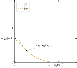
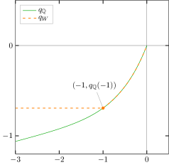
Figure 4: Illustration of Example 2.6. In the right picture, $q_{{\mathbb{Q}}}(\alpha)=q_{W}(\alpha)=\infty$ for all $\alpha>0$.

Example 2.7.

Define ${\mathbb{P}}={\mathbb{Q}}$ using $\gamma(0)=\hat{\gamma}(0)=0$, $\gamma(n)=\hat{\gamma}(n)=0.6\,\mathrm{e}^{n}$ for $n\in{\mathbb{N}}$. Then, we have ${\mathbb{P}}(\mathsf{b}^{n})={\mathbb{Q}}(\mathsf{b}^{n})\sim\mathrm{e}^{-\gamma(n)}$ and both bounds in (2.23) fail. Here, $q_{{\mathbb{P}}}$ is infinite for all $\alpha>1$, and $q_{{\mathbb{P}}}^{\prime}(1^{-})=\infty$. Each sequence of interest is exponentially tight and has a rate function that is good, but remains finite on an unbounded interval; in other words $\gamma_{-}=-\infty$.

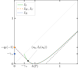
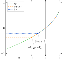
Figure 5: Illustration of Example 2.7. In the left picture, the dashed black asymptote is given by the equation $y=x-q_{{\mathbb{P}}}(1)$, and in the right picture, $q_{{\mathbb{P}}}(\alpha)=q_{W}(\alpha)=q_{V}(\alpha)=q_{R}(\alpha)=\infty$ for all $\alpha>1$.

Remark 2.8.

The possible lack of exponential tightness is specific to the case where ${\mathbb{P}}\neq{\mathbb{Q}}$; when ${\mathbb{P}}={\mathbb{Q}}$, our assumptions imply that all the random variables discussed in the paper are exponentially tight and that the corresponding rate functions are good. At the root of this fact is the exponential tightness of $(-\frac{1}{n}\ln{\mathbb{P}}_{n})_{n\in{\mathbb{N}}}$ with respect to ${\mathbb{P}}$ (Theorem  ‣ 1.1.iii). This exponential tightness will be derived as a consequence of (1.16), but it can also be seen directly: for any $M\geq 0$,

$${\mathbb{P}}\left\{x:-\frac{1}{n}\ln{\mathbb{P}}_{n}(x_{1}^{n})\geq M\right\}={\mathbb{P}}\{x:{\mathbb{P}}_{n}(x_{1}^{n})\leq\mathrm{e}^{-nM}\}\leq|{\cal A}|^{n}\mathrm{e}^{-Mn}.$$ (2.24)

We will come back to this point in Remark 5.3.

Remark 2.9.

This class of examples also allows for cases where the pressure $q_{{\mathbb{Q}}}$ is not differentiable — and hence where the Gärtner–Ellis route cannot provide the conclusions of Theorem  ‣ 1.1. Indeed, using the parameters $\gamma(n)=\hat{\gamma}(n)=\frac{n}{10}+4\ln(1+\frac{n}{4})$ yields a situation where $q_{{\mathbb{Q}}}$ is not differentiable at $\alpha_{0}\approx-0.1769$ and the rate functions are affine on an interval corresponding to the subdifferential of $q_{{\mathbb{Q}}}$ at $\alpha_{0}$.

3 Key estimates

This section is devoted to technical estimates on the distribution of $W_{n}$, $R_{n}$ and $V_{n}$ at large but finite $n\in{\mathbb{N}}$. We start with estimates for $W_{n}$ and then use those for our analysis of $R_{n}$ and $V_{n}$. In order to do so, we first need a convenient reformulation of our decoupling assumptions.

We show in Lemma B.2 that, at the cost of replacing $C_{n}$ with $C_{n}|{\cal A}|^{\tau_{n}}$ (which also satisfies (1.8)), 1.1 implies that for every $n\in{\mathbb{N}}$, $A\in{\cal F}_{n}$ and $B\in{\cal F}$,

$${\mathbb{P}}\left(A\cap T^{-n-\tau_{n}}B\right)\leq C_{n}{\mathbb{P}}(A){\mathbb{P}}(B).$$ (3.1)

In the same way, we show in Lemma B.3 that at the cost of replacing $C_{n}$ with $(\tau_{n}+1)C_{n}$, 1.1 implies that for every $n\in{\mathbb{N}}$, $A\in{\cal F}_{n}$ and $B\in{\cal F}$,

$$\max_{0\leq\ell\leq\tau_{n}}{\mathbb{P}}\left(A\cap T^{-n-\ell}B\right)\geq C_{n}^{-1}{\mathbb{P}}(A){\mathbb{P}}(B).$$ (3.2)

We shall freely use the form (3.1) of 1.1 and (3.2) of 1.1 throughout the paper.

3.1 Waiting times

Because $W_{n}:\Omega\times\Omega\to{\mathbb{N}}$ is $({\cal F}_{n}\otimes{\cal F})$-measurable, we will sometimes identify it to a function ${\cal A}^{n}\times\Omega\to{\mathbb{N}}$ denoted by the same symbol.

Lemma 3.1.

Assume ${\mathbb{Q}}$ satisfies 1.1. Then, for all $m,n\in{\mathbb{N}}$ and $u\in{\cal A}^{n}$,

$${\mathbb{Q}}\{y:W_{n}(u,y)=m\}\leq{\mathbb{Q}}_{n}(u)(1-C_{n}^{-1}{\mathbb{Q}}_{n}(u))^{\left\lfloor\frac{m-1}{n+\tau_{n}}\right\rfloor}$$ (3.3)

and

$${\mathbb{Q}}\{y:W_{n}(u,y)\geq m\}\leq(1-C_{n}^{-1}{\mathbb{Q}}_{n}(u))^{\left\lfloor\frac{m-1}{n+\tau_{n}}\right\rfloor}.$$ (3.4)

Proof.

Let us fix $n,m$ and $u$ as in the statement, and let $k:=\lfloor\tfrac{m-1}{n+\tau_{n}}\rfloor$. First, if $k=0$, then (3.4) is trivial and (3.3) holds since $\{y:W_{n}(u,y)=m\}\subseteq T^{1-m}[u]$ and ${\mathbb{Q}}$ is shift invariant.

Consider now the case $k\in{\mathbb{N}}$. In view of 1.1 (recall (3.2)) and shift invariance, we may inductively pick $k$ integers $0\leq\ell_{1},\ell_{2},\dots,\ell_{k}\leq\tau_{n}$ such that the nested intersections inductively defined by

$$A_{0}:=[u]\qquad\text{and}\qquad A_{j}:=[u]^{\mathsf{c}}\cap T^{-n-\ell_{j}}A_{j{-1}}$$

for $j=1,\dotsc,k$ satisfy ${\mathbb{Q}}\left([u]\cap T^{-n-\ell_{j}}A_{j-1}\right)\geq C_{n}^{-1}{\mathbb{Q}}_{n}(u){\mathbb{Q}}(A_{j-1})$, and thus also

$${\mathbb{Q}}(A_{j})={\mathbb{Q}}(A_{j-1})-{\mathbb{Q}}([u]\cap T^{-n-\ell_{j}}A_{j-1})\leq{\mathbb{Q}}(A_{j-1})(1-C_{n}^{-1}{\mathbb{Q}}_{n}(u)).$$ (3.5)

Iterating (3.5) starting from $A_{0}$ yields

$${\mathbb{Q}}(A_{k})\leq{\mathbb{Q}}_{n}(u)(1-C_{n}^{-1}{\mathbb{Q}}_{n}(u))^{k}.$$ (3.6)

Let $M:=\{m-jn-\sum_{i=1}^{j}\ell_{i}\}_{j=1}^{k}$. By construction, $kn+\sum_{i=1}^{k}\ell_{j}\leq k({n+\tau_{n}})<m$, so $M\subseteq[1,m-n]\subseteq[1,m-1]$. As a consequence,

$$\{y:W_{n}(u,y)=m\} =T^{1-m}[u]\cap\bigcap_{m^{\prime}=1}^{m-1}T^{1-m^{\prime}}[u]^{\mathsf{c}}$$

$$\subseteq T^{1-m}[u]\cap\bigcap_{m^{\prime}\in M}T^{1-m^{\prime}}[u]^{\mathsf{c}}$$

$$=T^{1-m+nk+\sum_{j=1}^{k}\ell_{j}}A_{k}.$$

Thus, by shift invariance and (3.6), we readily obtain (3.3). The proof of (3.4) is exactly the same with $A_{0}$ replaced by $\Omega$. ∎

Remark 3.2.

The bounds (3.5) and (3.6) are inspired by [Kon98, §2], and were already adapted to selective decoupling conditions in [CDEJR22]. It might be surprising that the upper bound (3.3) relies on the lower decoupling assumption 1.1. In fact, even if $\tau_{n}=0$ for all $n$, using 1.1 would yield ${\mathbb{Q}}(A_{k})\leq C_{n}^{k}{\mathbb{Q}}_{n}(u)(1-{\mathbb{Q}}_{n}(u))^{k}$ instead of (3.6); the extra factor of $C_{n}^{k}$ is too crude since we will be interested in the case where $k\gg n$. The opposite will happen in Lemma 3.4, where a lower bound will be proved using 1.1; see (3.13).

If ${\mathbb{Q}}_{n}(u)=0$, then ${\mathbb{Q}}\{y:W_{n}(u,y)=m\}\leq{\mathbb{Q}}(T^{1-m}[u])={\mathbb{Q}}_{n}(u)=0$ for all $m\in{\mathbb{N}}$, and thus $W_{n}(u,\cdot\,)$ is almost surely infinite. Conversely, if ${\mathbb{Q}}$ satisfies 1.1, the bound (3.4) ensures that $W_{n}(u,\cdot\,)$ is almost surely finite whenever ${\mathbb{Q}}_{n}(u)>0$. This last observation is at the heart of the next lemma.

Lemma 3.3.

Let $n\in{\mathbb{N}}$, let ${\mathbb{Q}}$ satisfy 1.1, and assume that ${\mathbb{P}}_{n}\ll{\mathbb{Q}}_{n}$. Then, the random variable $W_{n}$ is $({\mathbb{P}}\otimes{\mathbb{Q}})$-almost surely finite.

Proof.

This is a consequence of the decomposition

$$W_{n}(x,y)=\sum_{u\in{\cal A}^{n}}1_{[u]}(x)W_{n}(u,y),$$

the bound (3.4), and the absolute continuity assumption. ∎

We now turn to lower bounds on the distribution of $W_{n}(u,\cdot\,)$. The following lemma will be useful when $(1-C_{n}{\mathbb{Q}}_{n}(u))^{\left\lceil\frac{m-1}{n+\tau_{n}}\right\rceil}$ is close to $1$.

Lemma 3.4.

Assume ${\mathbb{Q}}$ satisfies 1.1. Then, for all $n,m\in{\mathbb{N}}$, and all $u\in{\cal A}^{n}$ such that $C_{n}{\mathbb{Q}}_{n}(u)\leq 1$,

$${\mathbb{Q}}\{y:W_{n}(u,y)=m\}\geq\frac{1}{n+\tau_{n}}{\mathbb{Q}}_{n}(u)\left(1-({n+\tau_{n}})\left(1-(1-C_{n}{\mathbb{Q}}_{n}(u))^{\left\lceil\frac{m-1}{n+\tau_{n}}\right\rceil}\right)\right).$$ (3.7)

Proof.

Let us fix $n,m$ and $u$ as in the statement. We first prove that it suffices to establish the bound

$$\begin{split}&{\mathbb{Q}}\{y:k({n+\tau_{n}})<W_{n}(u,y)\leq(k+1)({n+\tau_{n}})\}\\ &\qquad\qquad\geq{\mathbb{Q}}_{n}(u)\left(1-({n+\tau_{n}})\left(1-(1-C_{n}{\mathbb{Q}}_{n}(u))^{k}\right)\right)\end{split}$$ (3.8)

for all $k\in{\mathbb{N}}\cup\{0\}$. Since

$$\{y:W_{n}(u,y)=t+1\}\subseteq T^{-1}\{y:W_{n}(u,y)=t\}$$ (3.9)

for all $t\in{\mathbb{N}}$, the probability ${\mathbb{Q}}\{y:W_{n}(u,y)=t\}$ is nonincreasing in $t$. As a consequence, the left-hand side of (3.8) is bounded above by $({n+\tau_{n}}){\mathbb{Q}}\{y:W_{n}(u,y)=k({n+\tau_{n}})+1\}$, so (3.8) implies that

$${\mathbb{Q}}\{y:W_{n}(u,y)=1+k({n+\tau_{n}})\}\geq\frac{1}{n+\tau_{n}}{\mathbb{Q}}_{n}(u)\left(1-({n+\tau_{n}})\left(1-(1-C_{n}{\mathbb{Q}}_{n}(u))^{k}\right)\right).$$

By nonincreasingness, the same lower bound applies to ${\mathbb{Q}}\{y:W_{n}(u,y)=m\}$ for all $k$ such that $1+k({n+\tau_{n}})\geq m$, and thus (3.8) indeed implies (3.7).

We now establish (3.8). For every $y\in T^{1-(k+1)({n+\tau_{n}})}[u]=:A$ we have $W_{n}(u,y)\leq(k+1)({n+\tau_{n}})$, and for every $y\in\bigcap_{r=1}^{k({n+\tau_{n}})}T^{1-r}[u]^{\mathsf{c}}$ we have $W_{n}(u,y)>k({n+\tau_{n}})$. As a consequence,

$${\mathbb{Q}}\{y:k({n+\tau_{n}})<W_{n}(u,y)\leq(k+1)({n+\tau_{n}})\}\geq{\mathbb{Q}}\left(A\cap\bigcap_{r=1}^{k({n+\tau_{n}})}T^{1-r}[u]^{\mathsf{c}}\right).$$ (3.10)

We now write $\bigcap_{r=1}^{k({n+\tau_{n}})}T^{1-r}[u]^{\mathsf{c}}=\bigcap_{j=1}^{n+\tau_{n}}B_{j}$, where for $1\leq j\leq{n+\tau_{n}}$,

$$B_{j}:=\bigcap_{d=0}^{k-1}T^{1-d({n+\tau_{n}})-j}[u]^{\mathsf{c}}.$$

Notice that for each $j$, the events whose intersection defines $B_{j}$ are separated by “gaps” of size $\tau_{n}$, which will allow to use 1.1 below. By a union bound, (3.10) implies that

$${\mathbb{Q}}\{y:k({n+\tau_{n}})<W_{n}(u,y)\leq(k+1)({n+\tau_{n}})\} \geq{\mathbb{Q}}\left(A\cap\bigcap_{j=1}^{n+\tau_{n}}B_{j}\right)$$

$$={\mathbb{Q}}(A)-{\mathbb{Q}}\left(\bigcup_{j=1}^{n+\tau_{n}}(A\cap B_{j}^{\mathsf{c}})\right)$$

$$\geq{\mathbb{Q}}(A)-\sum_{j=1}^{n+\tau_{n}}{\mathbb{Q}}(A\cap B_{j}^{\mathsf{c}})$$

$$={\mathbb{Q}}(A)-\sum_{j=1}^{n+\tau_{n}}({\mathbb{Q}}(A)-{\mathbb{Q}}(A\cap B_{j})).$$

By shift invariance, ${\mathbb{Q}}(A)={\mathbb{Q}}_{n}(u)$, and thus the proof of (3.8) will be complete once we have shown that

$${\mathbb{Q}}(A\cap B_{j})\geq{\mathbb{Q}}_{n}(u)(1-C_{n}{\mathbb{Q}}_{n}(u))^{k}.$$ (3.11)

Fix $1\leq j\leq{n+\tau_{n}}$. We have

$$A\cap B_{j}=T^{1-j}\left(T^{j-(k+1)({n+\tau_{n}})}[u]\cap B_{1}\right)=T^{1-j}F_{k},$$ (3.12)

with $F_{0},\dots,F_{k}$ inductively defined by

$$F_{0}:=T^{j-n-\tau_{n}}[u]\qquad\text{and}\qquad F_{i}:=[u]^{\mathsf{c}}\cap T^{-n-\tau_{n}}F_{i-1}$$

for $i=1,\dotsc,k$. By 1.1 (recall (3.1)),

$${\mathbb{Q}}(F_{i})={\mathbb{Q}}(F_{i-1})-{\mathbb{Q}}([u]\cap T^{-n-\tau_{n}}F_{i-1})\geq{\mathbb{Q}}(F_{i-1})(1-C_{n}{\mathbb{Q}}_{n}(u)).$$

Iterating this bound starting with $F_{0}$ yields

$${\mathbb{Q}}(F_{k})\geq{\mathbb{Q}}_{n}(u)(1-C_{n}{\mathbb{Q}}_{n}(u))^{k}.$$ (3.13)

Combining this with (3.12) and using shift invariance establishes (3.11), as claimed. ∎

The next proposition makes precise the “cut-off” phenomenon sketched in (1.30) and uses the notation

$$U_{n}(s):=\left\{u\in{\cal A}^{n}:{\mathbb{Q}}_{n}(u)\leq{\mathrm{e}^{-ns}}\right\}$$ (3.14)

for $s>0$.

Proposition 3.5.

Suppose that ${\mathbb{Q}}$ satisfies 1.1 and 1.1, and let ${\mathbb{P}}\in{\cal P}_{\textnormal{inv}}(\Omega)$ satisfy ${\mathbb{P}}_{n}\ll{\mathbb{Q}}_{n}$ for all $n\in{\mathbb{N}}$. Then, for all $s>0$ and all $0<\delta\leq\epsilon<\tfrac{s}{2}$, we have, for all large enough $n$,

$$\begin{split}&{\mathbb{P}}\otimes{\mathbb{Q}}\{(x,y):\tfrac{1}{n}\ln W_{n}(x,y)\in B(s,\epsilon)\}\leq\mathrm{e}^{n(s+\epsilon)}\sum_{u\in U_{n}(s-\epsilon-\delta)}{\mathbb{Q}}_{n}(u){\mathbb{P}}_{n}(u)+\exp(-\mathrm{e}^{\frac{n\delta}{2}})\end{split}$$ (3.15)

and

$${\mathbb{P}}\otimes{\mathbb{Q}}\{(x,y):\tfrac{1}{n}\ln W_{n}(x,y)\in B(s,\epsilon)\}\geq\mathrm{e}^{n(s-\delta)}\sum_{u\in U_{n}(s+\delta)}{\mathbb{Q}}_{n}(u){\mathbb{P}}_{n}(u).$$ (3.16)

Proof.

The key idea in this proof is to show that, when $\frac{1}{n}\ln m\in B(s,\epsilon)$, the $\lfloor\tfrac{m-1}{n+\tau_{n}}\rfloor$-th power of $(1-C_{n}^{-1}{\mathbb{Q}}_{n}(u))$ in (3.3) vanishes superexponentially for all $u\notin U_{n}(s-\epsilon-\delta)$ as $n\to\infty$, and that the $\lceil\tfrac{m-1}{n+\tau_{n}}\rceil$-th power of $(1-C_{n}{\mathbb{Q}}_{n}(u))$ in (3.7) is very close to $1$ for all $u\in U_{n}(s+\delta)$ as $n\to\infty$. We fix $s$, $\epsilon$ and $\delta$ as in the statement and first note that

$${\mathbb{P}}\otimes{\mathbb{Q}}\{(x,y):\tfrac{1}{n}\ln W_{n}(x,y)\in B(s,\epsilon)\}=\sum_{u\in{\cal A}^{n}}{\mathbb{P}}_{n}(u){\mathbb{Q}}\{y:\tfrac{1}{n}\ln W_{n}(u,y)\in B(s,\epsilon)\}.$$ (3.17)

Proof of (3.15). Notice that $|\{m\in{\mathbb{N}}:\tfrac{1}{n}\ln m\in B(s,\epsilon)\}|\leq\mathrm{e}^{n(s+\epsilon)}$. Thus, using (3.17), the nonincreasingness of $t\mapsto{\mathbb{Q}}\{y:W_{n}(u,y)=t\}$ (recall (3.9)), and then Lemma 3.1, we find

$$\begin{split}{\mathbb{P}}\otimes{\mathbb{Q}}\{(x,y):\tfrac{1}{n}\ln W_{n}(x,y)\in B(s,\epsilon)\}&\leq\mathrm{e}^{n(s+\epsilon)}\sum_{u\in{\cal A}^{n}}{\mathbb{P}}_{n}(u){\mathbb{Q}}\{y:W_{n}(u,y)=m_{n}\}\\ &\leq\mathrm{e}^{n(s+\epsilon)}\sum_{u\in{\cal A}^{n}}{\mathbb{P}}_{n}(u){\mathbb{Q}}_{n}(u)(1-C_{n}^{-1}{\mathbb{Q}}_{n}(u))^{k_{n}},\end{split}$$ (3.18)

where $m_{n}:=\lceil\mathrm{e}^{n(s-\epsilon)}\rceil$ and $k_{n}:=\big{\lfloor}\frac{m_{n}-1}{n+\tau_{n}}\big{\rfloor}$. We now split the above sum into a sum over $U_{n}(s-\epsilon-\delta)$ and a sum over $U_{n}^{\mathsf{c}}(s-\epsilon-\delta)$. Clearly,

$$\sum_{u\in U_{n}(s-\epsilon-\delta)}{\mathbb{P}}_{n}(u){\mathbb{Q}}_{n}(u)(1-C_{n}^{-1}{\mathbb{Q}}_{n}(u))^{k_{n}}\leq\sum_{u\in U_{n}(s-\epsilon-\delta)}{\mathbb{P}}_{n}(u){\mathbb{Q}}_{n}(u),$$ (3.19)

while on the other hand,

$$\sum_{u\in U_{n}^{\mathsf{c}}(s-\epsilon-\delta)}{\mathbb{P}}_{n}(u){\mathbb{Q}}_{n}(u)(1-C_{n}^{-1}{\mathbb{Q}}_{n}(u))^{k_{n}}\leq(1-C_{n}^{-1}\mathrm{e}^{-n(s-\epsilon-\delta)})^{k_{n}}.$$ (3.20)

But using the inequality $(1-x)^{k_{n}}\leq\mathrm{e}^{-xk_{n}}$, we find

$$\mathrm{e}^{n(s+\epsilon)}(1-C_{n}^{-1}\mathrm{e}^{-n(s-\epsilon-\delta)})^{k_{n}} \leq\exp\left(n(s+\epsilon)-C_{n}^{-1}\mathrm{e}^{-n(s-\epsilon-\delta)}k_{n}\right)$$

$$\leq\exp(-\mathrm{e}^{\frac{n\delta}{2}})$$

for $n$ large enough, thanks to the fact that $k_{n}\geq\mathrm{e}^{n(s-\epsilon)-o(n)}$ and $C_{n}=\mathrm{e}^{o(n)}$ as $n\to\infty$. Therefore, using the estimates (3.19) and (3.20) in (3.18) indeed yields (3.15).

Proof of (3.16). This time, note that $|\{m\in{\mathbb{N}}:\tfrac{1}{n}\ln m\in(s-\epsilon,s]\}|\geq\tfrac{1}{2}\mathrm{e}^{ns}$ for $n$ large enough, and set $m_{n}:=\lfloor\mathrm{e}^{ns}\rfloor$ and $k_{n}:=\big{\lceil}\frac{m_{n}-1}{n+\tau_{n}}\big{\rceil}$. Then, by (3.17) and the nonincreasingness of $t\mapsto{\mathbb{Q}}\{y:W_{n}(u,y)=t\}$, we obtain

$${\mathbb{P}}\otimes{\mathbb{Q}}\{(x,y):\tfrac{1}{n}\ln W_{n}(x,y)\in B(s,\epsilon)\} \geq{\mathbb{P}}\otimes{\mathbb{Q}}\{(x,y):\tfrac{1}{n}\ln W_{n}(x,y)\in(s-\epsilon,s]\}$$

$$\geq\frac{\mathrm{e}^{ns}}{2}\sum_{u\in{\cal A}^{n}}{\mathbb{P}}_{n}(u){\mathbb{Q}}\{y:W_{n}(u,y)=m_{n}\}$$

$$\geq\frac{\mathrm{e}^{ns}}{2}\sum_{u\in U_{n}(s+\delta)}{\mathbb{P}}_{n}(u){\mathbb{Q}}\{y:W_{n}(u,y)=m_{n}\}.$$

Then, for $n$ large enough so that $C_{n}\mathrm{e}^{-n(s+\delta)}\leq 1$, we can apply Lemma 3.4 to every $u\in U_{n}(s+\delta)$, and we obtain that

$$\begin{split}&{\mathbb{P}}\otimes{\mathbb{Q}}\{(x,y):\tfrac{1}{n}\ln W_{n}(x,y)\in B(s,\epsilon)\}\\[5.69054pt] &\qquad\geq\frac{\mathrm{e}^{ns}}{2}\sum_{u\in U_{n}(s+\delta)}{\mathbb{P}}_{n}(u){\mathbb{Q}}_{n}(u)\left(({n+\tau_{n}})^{-1}-\left(1-(1-C_{n}{\mathbb{Q}}_{n}(u))^{k_{n}}\right)\right)\\ &\qquad\geq\frac{\mathrm{e}^{ns}}{2}\sum_{u\in U_{n}(s+\delta)}{\mathbb{P}}_{n}(u){\mathbb{Q}}_{n}(u)\left(({n+\tau_{n}})^{-1}-\left(1-(1-C_{n}\mathrm{e}^{-n(s+\delta)})^{k_{n}}\right)\right).\end{split}$$ (3.21)

Notice that by Bernoulli’s inequality, $(1-x)^{k_{n}}\geq 1-xk_{n}$ for all $x\leq 1$. As a consequence, for all $n$ large enough,

$$(1-C_{n}\mathrm{e}^{-n(s+\delta)})^{k_{n}}\geq 1-C_{n}\mathrm{e}^{-n(s+\delta)}k_{n}\geq 1-\mathrm{e}^{-\frac{n\delta}{2}},$$

where we have used that $k_{n}\leq\mathrm{e}^{ns+o(n)}$ and $C_{n}=\mathrm{e}^{o(n)}$. Substitution into (3.21) yields

$${\mathbb{P}}\otimes{\mathbb{Q}}\{(x,y):\tfrac{1}{n}\ln W_{n}(x,y)\in B(s,\epsilon)\} \geq\frac{\mathrm{e}^{ns}}{2}\sum_{u\in U_{n}(s+\delta)}{\mathbb{P}}_{n}(u){\mathbb{Q}}_{n}(u)\left(({n+\tau_{n}})^{-1}-\mathrm{e}^{-\frac{n\delta}{2}}\right),$$

from which the lower bound (3.16) readily follows when $n$ is large enough. ∎

3.2 From waiting times to return times

Lemma 3.6.

Assume ${\mathbb{P}}$ satisfies 1.1. Then, for all $s>0$ and all $0<\epsilon<s$, we have, for all large enough $n$,

$${\mathbb{P}}\{x:\tfrac{1}{n}\ln R_{n}(x)\in B(s,\epsilon)\}\leq C_{n}\sum_{u\in{\cal A}^{n}}{\mathbb{P}}_{n}(u){\mathbb{P}}\{x:\tfrac{1}{n}\ln W_{n}(u,x)\in B(s,2\epsilon)\}$$

and

$${\mathbb{P}}\{x:\tfrac{1}{n}\ln V_{n}(x)\in B(s,\epsilon)\}\leq C_{n}\sum_{u\in{\cal A}^{n}}{\mathbb{P}}_{n}(u){\mathbb{P}}\{x:\tfrac{1}{n}\ln W_{n}(u,x)\in B(s,2\epsilon)\}.$$

Proof.

Fix $s>\epsilon>0$, fix $n\in{\mathbb{N}}$ large enough so that

$$\mathrm{e}^{n(s-\epsilon)}>{n+\tau_{n}}-1\qquad\text{and}\qquad\mathrm{e}^{n(s-2\epsilon)}\leq\mathrm{e}^{n(s-\epsilon)}+1-n-\tau_{n},$$ (3.22)

and fix $u\in{\cal A}^{n}$. Then, for all $x\in[u]$ such that $\frac{1}{n}\ln R_{n}(x)\in B(s,\epsilon)$, we have $R_{n}(x)=W_{n}(u,Tx)\in(\mathrm{e}^{n(s-\epsilon)},\mathrm{e}^{n(s+\epsilon)})$. The first condition in (3.22) implies that $W_{n}(u,T^{n+\tau_{n}}x)=W_{n}(u,Tx)+1-n-\tau_{n}$ for all such $x$, so that, also using the second condition in (3.22),

$$W_{n}(u,T^{n+\tau_{n}}x)\in(\mathrm{e}^{n(s-\epsilon)}+1-n-\tau_{n},\mathrm{e}^{n(s+\epsilon)}+1-n-\tau_{n})\subset(\mathrm{e}^{n(s-2\epsilon)},\mathrm{e}^{n(s+2\epsilon)}).$$

As a consequence, by 1.1,

$${\mathbb{P}}([u]\cap\{x:\tfrac{1}{n}\ln{R}_{n}(x)\in B(s,\epsilon)\}) \leq{\mathbb{P}}([u]\cap\{x:\tfrac{1}{n}\ln W_{n}(u,T^{n+\tau_{n}}x)\in B(s,2\epsilon)\})$$

$$\leq C_{n}{\mathbb{P}}_{n}(u){\mathbb{P}}\{x:\tfrac{1}{n}\ln W_{n}(u,x)\in B(s,2\epsilon)\}.$$

Taking the sum over $u\in{\cal A}^{n}$ proves the desired bound for $R_{n}$. The proof of the bound for $V_{n}$ is almost identical: for all $x\in[u]$ such that $\frac{1}{n}\ln V_{n}(x)\in B(s,\epsilon)$, we have this time $W_{n}(u,T^{n}x)\in(\mathrm{e}^{n(s-\epsilon)},\mathrm{e}^{n(s+\epsilon)})$, so that $W_{n}(u,T^{n+\tau_{n}}x)\in(\mathrm{e}^{n(s-\epsilon)}-\tau_{n},\mathrm{e}^{n(s+\epsilon)}-\tau_{n})\subset(\mathrm{e}^{n(s-2\epsilon)},\mathrm{e}^{n(s+2\epsilon)})$. The remainder of the argument is unchanged. ∎

Lemma 3.7.

Assume ${\mathbb{P}}$ satisfies 1.1. Then, for all $s>0$ and all $0<\epsilon<s$, we have, for all large enough $n$,

$${\mathbb{P}}\{x:\tfrac{1}{n}\ln R_{n}(x)\in B(s,\epsilon)\}\geq\frac{C_{n}^{-1}}{n+\tau_{n}}\sum_{u\in{\cal A}^{n}}{\mathbb{P}}_{n}(u){\mathbb{P}}\{x:\tfrac{1}{n}\ln W_{n}(u,x)\in B(s,\tfrac{1}{2}\epsilon)\}$$

and

$${\mathbb{P}}\{x:\tfrac{1}{n}\ln V_{n}(x)\in B(s,\epsilon)\}\geq\frac{C_{n}^{-1}}{1+\tau_{n}}\sum_{u\in{\cal A}^{n}}{\mathbb{P}}_{n}(u){\mathbb{P}}\{x:\tfrac{1}{n}\ln W_{n}(u,x)\in B(s,\tfrac{1}{2}\epsilon)\}.$$

Proof.

We first prove the statement concerning $R_{n}$. Fix $s>\epsilon>0$, fix $n$ large enough so that

$$\mathrm{e}^{n(s+\frac{1}{2}\epsilon)}+{n+\tau_{n}}-1<\mathrm{e}^{n(s+\epsilon)},$$ (3.23)

and fix $u\in{\cal A}^{n}$. By 1.1, there exists $0\leq\ell\leq\tau_{n}$ such that the set

$$A_{u}:=[u]\cap T^{-n-\ell}\{x:\tfrac{1}{n}\ln W_{n}(u,x)\in B(s,\tfrac{1}{2}\epsilon)\}$$

satisfies

$${\mathbb{P}}(A_{u})\geq C_{n}^{-1}{\mathbb{P}}_{n}(u){\mathbb{P}}\{x:\tfrac{1}{n}\ln W_{n}(u,x)\in B(s,\tfrac{1}{2}\epsilon)\}.$$ (3.24)

We now claim that

$$A_{u}\subseteq\bigcup_{j=1}^{n+\tau_{n}}T^{1-j}\{x:\tfrac{1}{n}\ln R_{n}(x)\in B(s,\epsilon)\}.$$ (3.25)

To prove (3.25), take an arbitrary $x\in A_{u}$, and let $m:=W_{n}(u,T^{n+\ell}x)$, which, by the definition of $A_{u}$, satisfies $\frac{1}{n}\ln m\in B(s,\tfrac{1}{2}\epsilon)$. Then, the set $I:=\{i\in{\mathbb{N}}:x_{i}^{i+n-1}=u\}$ contains $1$ and $n+\ell+m$, but excludes $\{n+\ell+1,n+\ell+2,\dotsc,n+\ell+m-1\}$. Hence, with $j:=\max\{i\in I:i\leq n+\ell\}$ we find $R_{n}(T^{j-1}x)=n+\ell+m-j\in[m,m+n+\tau_{n}-1]$, so by (3.23) we obtain (3.25).

By taking the union over $u\in{\cal A}^{n}$ in the left-hand side of (3.25), and using shift invariance to bound the probability of the right-hand side, we obtain

$$\sum_{u\in{\cal A}^{n}}{\mathbb{P}}(A_{u})={\mathbb{P}}\left(\bigcup_{u\in{\cal A}^{n}}A_{u}\right)\leq(n+\tau_{n}){\mathbb{P}}\{x:\tfrac{1}{n}\ln R_{n}(x)\in B(s,\epsilon)\}.$$ (3.26)

In view of (3.24), we have completed the proof of the statement about $R_{n}$.

To adapt the proof for $V_{n}$, it suffices to replace the definition of $j$ with $j:=\max\{i\in I:i\leq 1+\ell\}$; then $V_{n}(T^{j-1}x)=1+\ell+m-j\in[m,m+\tau_{n}]$ and the same arguments apply, with the factor $(n+\tau_{n})$ replaced by $(1+\tau_{n})$ in (3.26). ∎

Lemma 3.8.

Assume ${\mathbb{P}}$ satisfies 1.1. Then, for every $n\in{\mathbb{N}}$, the random variables $R_{n}$ and $V_{n}$ are ${\mathbb{P}}$-almost surely finite.

Proof.

In view of (3.4), the random variable $W_{n}(u,\cdot\,)$ is ${\mathbb{P}}$-almost surely finite for every fixed $u\in{\cal A}^{n}$ with ${\mathbb{P}}_{n}(u)>0$. By shift invariance, so is $W_{n}(u,\cdot\,)\circ T^{k}$ for each $k$. In view of the expressions

$$R_{n}(x) =\sum_{u\in{\cal A}^{n}}1_{[u]}(x)W_{n}(u,Tx),$$

$$V_{n}(x) =\sum_{u\in{\cal A}^{n}}1_{[u]}(x)W_{n}(u,T^{n}x),$$

the conclusion is immediate. ∎

Remark 3.9.

An alternative way of showing that $R_{n}$ and $V_{n}$ are almost surely finite is to use the Poincaré recurrence theorem, see e.g. Theorem 1.4 in [Wal82].

4 The weak LDP and Ruelle–Lanford functions

We now briefly recall some terminology from the theory of large deviations, limiting ourselves to sequences of real-valued random variables. See for example [DS89, Ell06, DZ09] for proper introductions to the field. Let $(Z_{n})_{n\in{\mathbb{N}}}$ be a sequence of (almost surely finite) real-valued random variables on a probability space $(\Omega_{*},{\mathbb{P}}_{*})$. The cases of interest will be

• $\Omega_{*}=\Omega\times\Omega$, ${\mathbb{P}}_{*}={\mathbb{P}}\otimes{\mathbb{Q}}$ and $Z_{n}=\frac{1}{n}\ln W_{n}$ for Theorem A;

• $\Omega_{*}=\Omega$, ${\mathbb{P}}_{*}={\mathbb{P}}$, with $Z_{n}=-\frac{1}{n}\ln{\mathbb{Q}}_{n}$, $Z_{n}=\frac{1}{n}\ln V_{n}$ and $Z_{n}=\frac{1}{n}\ln R_{n}$ for, respectively, Theorems  ‣ 1.1, B and C.

The sequence $(Z_{n})_{n\in{\mathbb{N}}}$ is said to satisfy the large deviation principle (LDP) if there exists a lower semicontinuous function $I:{\mathbb{R}}\to[0,\infty]$ such that

$$-\inf_{s\in O}I(s)\leq\liminf_{n\to\infty}\frac{1}{n}\ln{\mathbb{P}}_{*}\{x:Z_{n}(x)\in O\}$$ (4.1)

for every open set $O\subseteq{\mathbb{R}}$ and

$$\limsup_{n\to\infty}\frac{1}{n}\ln{\mathbb{P}}_{*}\{x:Z_{n}(x)\in\Gamma\}\leq-\inf_{{s}\in\Gamma}I({s})$$ (4.2)

for every closed set $\Gamma\subseteq{\mathbb{R}}$. The bounds (4.1) and (4.2) are respectively called the large-deviation lower bound and the large-deviation upper bound, and the function $I$ is called the rate function. Following standard terminology, we say that $I$ is a good rate function if it properly diverges as $s\to\pm\infty$. We also recall that the large-deviation upper bound applied to the set ${\mathbb{R}}$ implies that $\inf_{s\in{\mathbb{R}}}I(s)=0$. Ubiquitous in the theory of large deviations is the question of whether the rate function is convex and can be expressed as the Legendre–Fenchel transform of the corresponding pressure. A detailed analysis of these considerations for the random variables of interest is postponed to Section 5.

Our analysis will require additional vocabulary which is discussed e.g. in [DZ09, §1.2]. The sequence $(Z_{n})_{n\in{\mathbb{N}}}$ is said to satisfy the weak large deviation principle if (4.1) holds for all open sets $O\subseteq{\mathbb{R}}$, and (4.2) holds for all compact sets $\Gamma\Subset{\mathbb{R}}$. We shall sometimes refer to the standard LDP as the full LDP when we need to emphasize the contrast to the weak LDP used as a stepping stone towards the full LDP. The following notion will play a role in doing so: the sequence $(Z_{n})_{n\in{\mathbb{N}}}$ is said to be exponentially tight if, for every $\beta\in{\mathbb{R}}$, there exists $M>0$ such that ${\mathbb{P}}_{*}\{x:Z_{n}(x)\notin[-M,M]\}\leq\mathrm{e}^{-\beta n}$ for all $n$ large enough. To be more precise, we will appeal to the two following facts for real-valued sequences. First, if the weak LDP holds and the sequence is exponentially tight, then the full LDP holds with a good rate function. Second, if the full LDP holds with a good rate function, then the sequence is exponentially tight. While all our LDPs are full, and while exponential tightness does play a role in our analysis, we emphasize that the sequence $(\tfrac{1}{n}\ln W_{n})_{n\in{\mathbb{N}}}$ need not be exponentially tight, as illustrated in Section 2.5.

As mentioned, we will first prove the weak LDP. We will do so using Ruelle–Lanford (RL) functions. We introduce the lower RL function $\underline{I}:{\mathbb{R}}\to[0,\infty]$ defined by

$$\underline{I}(s):=-\lim_{\epsilon\to 0}\liminf_{n\to\infty}\frac{1}{n}\ln{\mathbb{P}}_{*}\{x:Z_{n}(x)\in B(s,\epsilon)\},$$

and the upper RL function $\overline{I}$ : ${\mathbb{R}}\to[0,\infty]$ defined by

$$\overline{I}(s):=-\lim_{\epsilon\to 0}\limsup_{n\to\infty}\frac{1}{n}\ln{\mathbb{P}}_{*}\{x:Z_{n}(x)\in B(s,\epsilon)\}.$$

It follows from their definition that $\overline{I}$ and $\underline{I}$ are lower semicontinuous, and that $\overline{I}\leq\underline{I}$. Moreover, the weak LDP holds if and only if we have the equality

$$\underline{I}(s)=\overline{I}(s)$$ (4.3)

for every $s\in{\mathbb{R}}$; see e.g. [DZ09, §4.1.2] or [CJPS19, §3.2]. The common value in (4.3) must then coincide with $I(s)$.

The core of this section is devoted to proving the weak LDP for the sequences of interest via the validity of (4.3). To be more precise, for each sequence, both RL functions are shown to be equal to the proposed rate function, as detailed in Table 2. We consider separately the case $s>0$ in Section 4.1 and the case $s=0$ in Section 4.2, noting that the case $s<0$ is trivial by mere nonnegativity of the random variables under study. We denote by $\underline{I}_{W}$, $\underline{I}_{V}$ and $\underline{I}_{R}$ (resp. $\overline{I}_{W}$, $\overline{I}_{V}$ and $\overline{I}_{R}$) the lower (resp. upper) RL functions associated with our sequences.

Rand. var.	Space	Assumptions	Proposed rate	(4.3) for $s>0$	(4.3) for $s=0$
$\tfrac{1}{n}\ln W_{n}$	$(\Omega\times\Omega,{\mathbb{P}}\otimes{\mathbb{Q}})$	admissibility	$I_{W}$ (1.19)	Prop. 4.2	Prop. 4.4
$\tfrac{1}{n}\ln V_{n}$	$(\Omega,{\mathbb{P}})$	1.1, 1.1	$I_{V}$ (1.22)	Prop. 4.3	Prop. 4.5
$\tfrac{1}{n}\ln R_{n}$	$(\Omega,{\mathbb{P}})$	1.1, 1.1, 1.4	$I_{R}$ (1.25)	Prop. 4.3	Prop. 4.7

Table 2: Assumptions, proposed rate function and references to where the key equality (4.3) is established for the three weak LDPs to be proved.

4.1 At positive values

Our first goal is to prove equality of the upper and lower Ruelle–Lanford functions at positive values of $s$. We start with the RL functions $\underline{I}_{W}$ and $\overline{I}_{W}$ of the sequence $(\tfrac{1}{n}\ln W_{n})_{n\in{\mathbb{N}}}$. Most of the work to show that $\underline{I}_{W}(s)=\overline{I}_{W}(s)$ when $s>0$ was done in Section 3.1: in view of Proposition 3.5, it only remains to estimate the quantity

$$J_{n}(s):=\sum_{u\in U_{n}(s)}\mathrm{e}^{\ln{\mathbb{Q}}_{n}(u)}{\mathbb{P}}_{n}(u)=\int_{[s,\infty)}\mathrm{e}^{-rn}\mathop{\mathrm{\mathstrut d}}\nolimits\!\mu_{n}(r),$$ (4.4)

where $\mu_{n}$ is the distribution of $-\frac{1}{n}\ln{\mathbb{Q}}_{n}$ with respect to ${\mathbb{P}}$, and where $U_{n}(s)$ was defined in (3.14). The integral in (4.4) allows to express the limiting behavior of $J_{n}$ in terms of the rate function $I_{{\mathbb{Q}}}$ of Theorem  ‣ 1.1, as shown by the following straightforward variation of Varadhan’s lemma.

Lemma 4.1.

Assume $({\mathbb{P}},{\mathbb{Q}})$ is admissible. Then, for all $s>0$,

$$\sup_{r>s}(-r-I_{{\mathbb{Q}}}(r))\leq\liminf_{n\to\infty}\frac{1}{n}\ln J_{n}(s)\leq\limsup_{n\to\infty}\frac{1}{n}\ln J_{n}(s)\leq\sup_{r\geq s}(-r-I_{{\mathbb{Q}}}(r)).$$

Proof.

Let us fix $s>0$. For the lower bound, note that for every choice of $r>s$ and $0<\epsilon<r-s$,

$$\liminf_{n\to\infty}\frac{1}{n}\ln J_{n}(s) \geq\liminf_{n\to\infty}\frac{1}{n}\ln\int_{B(r,\epsilon)}\mathrm{e}^{-r^{\prime}n}\mathop{\mathrm{\mathstrut d}}\nolimits\!\mu_{n}(r^{\prime})$$

$$\geq-r-\epsilon+\liminf_{n\to\infty}\frac{1}{n}\ln\mu_{n}(B(r,\epsilon))$$

$$\geq-r-\epsilon-I_{{\mathbb{Q}}}(r),$$

where we have used the large-deviation lower bound of Theorem  ‣ 1.1. For the upper bound, let $\beta:=\inf_{r\geq s}(r+I_{{\mathbb{Q}}}(r))\in[s,\infty)$. Then,

$$J_{n}(s) =\int_{[s,\beta]}\mathrm{e}^{-rn}\mathop{\mathrm{\mathstrut d}}\nolimits\!\mu_{n}(r)+\int_{(\beta,\infty)}\mathrm{e}^{-rn}\mathop{\mathrm{\mathstrut d}}\nolimits\!\mu_{n}(r)\leq\int_{[s,\beta]}\mathrm{e}^{-rn}\mathop{\mathrm{\mathstrut d}}\nolimits\!\mu_{n}(r)+\mathrm{e}^{-\beta n}.$$

As a consequence, it suffices to show that

$$\limsup_{n\to\infty}\frac{1}{n}\int_{[s,\beta]}\mathrm{e}^{-rn}\mathop{\mathrm{\mathstrut d}}\nolimits\!\mu_{n}(r)\leq-\beta,$$ (4.5)

which, since $[s,\beta]$ is compact, follows from a standard covering argument, see e.g. Lemma 4.3.6 in [DZ09] or the proof of Proposition C.1.iv below. ∎

Proposition 4.2.

Assume the pair $({\mathbb{P}},{\mathbb{Q}})$ is admissible. Then, for all $s>0$, the RL functions for $(\frac{1}{n}\ln W_{n})_{n\in{\mathbb{N}}}$ with respect to ${\mathbb{P}}\otimes{\mathbb{Q}}$ satisfy

$$\underline{I}_{W}(s)=\overline{I}_{W}(s)=-s+\inf_{r\geq s}(r+I_{{\mathbb{Q}}}(r)).$$ (4.6)

Proof.

Let $s>0$. By Proposition 3.5 and Lemma 4.1, we find that for all $0<\delta\leq\epsilon<\tfrac{1}{2}s$,

$$\limsup_{n\to\infty}\frac{1}{n}\ln{\mathbb{P}}\otimes{\mathbb{Q}}\{(x,y):\tfrac{1}{n}\ln W_{n}(x,y)\in B(s,\epsilon)\}\leq s+\epsilon-\inf_{r\geq s-\epsilon-\delta}(r+I_{{\mathbb{Q}}}(r))$$ (4.7)

and

$$\liminf_{n\to\infty}\frac{1}{n}\ln{\mathbb{P}}\otimes{\mathbb{Q}}\{(x,y):\tfrac{1}{n}\ln W_{n}(x,y)\in B(s,\epsilon)\}\geq s-\delta-\inf_{r>s+\delta}(r+I_{{\mathbb{Q}}}(r)).$$ (4.8)

By taking the limit as $\delta\to 0$ first and then $\epsilon\to 0$ in (4.7), and since $I_{{\mathbb{Q}}}$ is lower semicontinuous, we obtain that $-\overline{I}_{W}(s)\leq s-\inf_{r\geq s}(r+I_{{\mathbb{Q}}}(r))$. Taking the same limits in (4.8) yields $-\underline{I}_{W}(s)\geq s-\inf_{r>s}(r+I_{{\mathbb{Q}}}(r))$. We then have

$$-s+\inf_{r\geq s}(r+I_{{\mathbb{Q}}}(r))\leq\overline{I}_{W}(s)\leq\underline{I}_{W}(s)\leq-s+\inf_{r>s}(r+I_{{\mathbb{Q}}}(r)).$$ (4.9)

For all $s^{\prime}\in(0,s)$, the last inequality in (4.9) applied to $s^{\prime}$ yields

$$\underline{I}_{W}(s^{\prime})\leq-s^{\prime}+\inf_{r>s^{\prime}}(r+I_{{\mathbb{Q}}}(r))\leq-s^{\prime}+\inf_{r\geq s}(r+I_{{\mathbb{Q}}}(r)).$$

Since $\underline{I}_{W}$ is lower semicontinuous (as a RL function), this in turn implies that

$$\underline{I}_{W}(s)\leq\liminf_{s^{\prime}\uparrow s}\underline{I}_{W}(s^{\prime})\leq-s+\inf_{r\geq s}(r+I_{{\mathbb{Q}}}(r)),$$

so the first three quantities in (4.9) are actually equal, as desired. ∎

Proposition 4.3.

Assume ${\mathbb{P}}$ satisfies 1.1 and 1.1. Then, for all $s>0$, the RL functions for $(\frac{1}{n}\ln R_{n})_{n\in{\mathbb{N}}}$ and $(\frac{1}{n}\ln V_{n})_{n\in{\mathbb{N}}}$ with respect to ${\mathbb{P}}$ satisfy

$$\underline{I}_{R}(s)=\overline{I}_{R}(s)=-s+\inf_{r\geq s}(r+I_{{\mathbb{P}}}(r))$$

and

$$\underline{I}_{V}(s)=\overline{I}_{V}(s)=-s+\inf_{r\geq s}(r+I_{{\mathbb{P}}}(r)).$$

Proof.

Let $s>0$. First, we remark that Proposition 4.2 applies to the admissible pair $({\mathbb{P}},{\mathbb{P}})$, so that $\overline{I}_{W}(s)=\underline{I}_{W}(s)=-s+\inf_{r\geq s}(r+I_{{\mathbb{P}}}(r))$. Then, Lemma 3.6 implies that $\overline{I}_{R}(s)\geq\overline{I}_{W}(s)$ and $\overline{I}_{V}(s)\geq\overline{I}_{W}(s)$; recall also (3.17). In the same way, Lemma 3.7 implies that $\underline{I}_{R}(s)\leq\underline{I}_{W}(s)$ and $\underline{I}_{V}(s)\leq\underline{I}_{W}(s)$. Since also $\overline{I}_{R}\leq\underline{I}_{R}$ and $\overline{I}_{V}\leq\underline{I}_{V}$, the proof is complete. ∎

4.2 At the origin

In this subsection, we prove that, for each of the sequences $(\frac{1}{n}\ln W_{n})_{n\in{\mathbb{N}}}$, $(\frac{1}{n}\ln V_{n})_{n\in{\mathbb{N}}}$ and $(\frac{1}{n}\ln R_{n})_{n\in{\mathbb{N}}}$, the upper and lower RL functions match at $s=0$. We recall that the limit

$$q_{{\mathbb{Q}}}(-1)=\lim_{n\to\infty}\frac{1}{n}\ln\sum_{u\in{\cal A}^{n}}{\mathbb{P}}_{n}(u){\mathbb{Q}}_{n}(u)$$ (4.10)

exists for any admissible pair $({\mathbb{P}},{\mathbb{Q}})$ by Theorem  ‣ 1.1.ii.

Proposition 4.4.

If the pair $({\mathbb{P}},{\mathbb{Q}})$ is admissible, then

$$\underline{I}_{W}(0)=\overline{I}_{W}(0)=-q_{{\mathbb{Q}}}(-1)=\inf_{r\geq 0}(r+I_{{\mathbb{Q}}}(r)).$$ (4.11)

Proof.

For all $\epsilon>0$ and $n\in{\mathbb{N}}$,

$${\mathbb{P}}\otimes{\mathbb{Q}}\{(x,y):\tfrac{1}{n}\ln W_{n}(x,y)\in B(0,\epsilon)\}\geq{\mathbb{P}}\otimes{\mathbb{Q}}\{(x,y):W_{n}(x,y)=1\}=\sum_{u\in{\cal A}^{n}}{\mathbb{P}}_{n}(u){\mathbb{Q}}_{n}(u).$$

In view of (4.10) and the definition of $\underline{I}_{W}$, we have $\underline{I}_{W}(0)\leq-q_{{\mathbb{Q}}}(-1)$. To obtain the opposite inequality for $\overline{I}_{W}(0)$, observe that

$${\mathbb{P}}\otimes{\mathbb{Q}}\{(x,y):W_{n}(x,y)=k\}\leq{\mathbb{P}}\otimes{\mathbb{Q}}\{(x,y):x_{1}^{n}=y_{1+k}^{n+k}\}=\sum_{u\in{\cal A}^{n}}{\mathbb{P}}_{n}(u){\mathbb{Q}}_{n}(u)$$

for every $u\in{\cal A}^{n}$, $n\in{\mathbb{N}}$ and $k\in{\mathbb{N}}$. Therefore, a union bound gives, for every $\epsilon>0$,

$${\mathbb{P}}\otimes{\mathbb{Q}}\{(x,y):W_{n}(x,y)\leq\mathrm{e}^{\epsilon n}\}\leq\mathrm{e}^{\epsilon n}\sum_{u\in{\cal A}^{n}}{\mathbb{P}}_{n}(u){\mathbb{Q}}_{n}(u).$$

By (4.10) and the definition of $\overline{I}_{W}$, we conclude that $\overline{I}_{W}(0)\geq-q_{{\mathbb{Q}}}(-1)$. Since also $\underline{I}_{W}(0)\geq\overline{I}_{W}(0)$ we have thus established the first two equalities in (4.11).

To complete the proof, it remains to observe that, since $I_{{\mathbb{Q}}}(r)=\infty$ for all $r<0$, and since $q_{{\mathbb{Q}}}=I_{{\mathbb{Q}}}^{*}$ by Theorem  ‣ 1.1.ii,

$$\inf_{r\geq 0}(r+I_{{\mathbb{Q}}}(r))=\inf_{r\in{\mathbb{R}}}(r+I_{{\mathbb{Q}}}(r))=-\sup_{r\in{\mathbb{R}}}(-r-I_{{\mathbb{Q}}}(r))=-q_{{\mathbb{Q}}}(-1),$$ (4.12)

which establishes the last identity in (4.11). ∎

Proposition 4.5.

If ${\mathbb{P}}$ satisfies 1.1 and 1.1, then

$$\underline{I}_{V}(0)=\overline{I}_{V}(0)=-q_{{\mathbb{P}}}(-1)=\inf_{r\geq 0}(r+I_{{\mathbb{P}}}(r)).$$ (4.13)

Proof.

The stated assumptions allow to apply Theorem  ‣ 1.1 to the pair $({\mathbb{P}},{\mathbb{P}})$, and in particular its consequences (4.10) and (4.12) with ${\mathbb{Q}}={\mathbb{P}}$. Since the third equality in (4.13) is a special case of (4.12), and since $\overline{I}_{V}(0)\leq\underline{I}_{V}(0)$ by definition, it suffices to establish the inequalities $\underline{I}_{V}(0)\leq-q_{{\mathbb{P}}}(-1)$ and $\overline{I}_{V}(0)\geq-q_{{\mathbb{P}}}(-1)$ in order to complete the proof. To this end, we let $\epsilon>0$ be arbitrary and restrict our attention to $n$ large enough so that $\min\{n,\mathrm{e}^{\epsilon n}\}>\tau_{n}+1$.

For each $u\in{\cal A}^{n}$, 1.1 implies that there is $0\leq\ell\leq\tau_{n}$ such that ${\mathbb{P}}([u]\cap T^{-n-\ell}[u])\geq C_{n}^{-1}{\mathbb{P}}_{n}(u)^{2}$. Since $[u]\cap\{x:V_{n}(x)\leq\tau_{n}+1\}\supseteq[u]\cap T^{-n-\ell}[u]$, this in turn implies that

$${\mathbb{P}}\{x:V_{n}(x)<\mathrm{e}^{\epsilon n}\}\geq{\mathbb{P}}\{x:V_{n}(x)\leq\tau_{n}+1\}\geq C_{n}^{-1}\sum_{u\in{\cal A}^{n}}{\mathbb{P}}_{n}(u)^{2}.$$

Combining this with (4.10) for ${\mathbb{Q}}={\mathbb{P}}$ establishes the inequality $\underline{I}_{V}(0)\leq-q_{{\mathbb{P}}}(-1)$.

On the other hand, for each $k\in{\mathbb{N}}$,

$$\{x:V_{n}(x)=k\}\subseteq\bigcup_{u\in{\cal A}^{n}}[u]\cap T^{1-n-k}[u]\subseteq\bigcup_{v\in{\cal A}^{n-\tau_{n}}}[v]\cap T^{1-n-k}[v].$$

Assuming without loss of generality that the sequence $(\tau_{n})_{n\in{\mathbb{N}}}$ is nondecreasing (so in particular $\tau_{n-\tau_{n}}\leq\tau_{n}$), we obtain from 1.1 that

$${\mathbb{P}}\{x:V_{n}(x)=k\}\leq C_{n-\tau_{n}}\sum_{v\in{\cal A}^{n-\tau_{n}}}{\mathbb{P}}_{n-\tau_{n}}(v)^{2}.$$

Considering the union over $k=1,2,\dotsc,\lceil\mathrm{e}^{\epsilon n}\rceil-1$, we further obtain

$$\begin{split}\limsup_{n\to\infty}\frac{1}{n}\ln{\mathbb{P}}\{x:V_{n}(x)<\mathrm{e}^{\epsilon n}\}&\leq\limsup_{n\to\infty}\frac{1}{n}\ln\left(\mathrm{e}^{\epsilon n}C_{n-\tau_{n}}\sum_{v\in{\cal A}^{n-\tau_{n}}}{\mathbb{P}}_{n-\tau_{n}}(v)^{2}\right)\\ &=\epsilon+\limsup_{n\to\infty}\frac{1}{n}\ln\sum_{u\in{\cal A}^{n}}{\mathbb{P}}_{n}(u)^{2},\end{split}$$ (4.14)

where we have used that $\lim_{n\to\infty}\frac{n-\tau_{n}}{n}=1$. Combining this with (4.10) for ${\mathbb{Q}}={\mathbb{P}}$ establishes the inequality $\overline{I}_{V}(0)\geq-q_{{\mathbb{P}}}(-1)$, so the proof is complete. ∎

Let us now turn to $\underline{I}_{R}(0)$ and $\overline{I}_{R}(0)$, whose comparison is significantly more involved. We start with a technical lemma.

Lemma 4.6.

If ${\mathbb{P}}$ satisfies 1.1 and 1.1, then

$$\gamma_{+}=\lim_{n\to\infty}\frac{1}{n}\sup_{u\in{\cal A}^{n}}\ln{\mathbb{P}}_{n}(u)\geq q_{{\mathbb{P}}}(-1).$$ (4.15)

Proof.

From Theorem  ‣ 1.1.iii.b, we know that the limit superior in the definition (1.12) of $\gamma_{+}$ is actually a limit, which is the first equality in (4.15). We now prove the inequality, noting that, by Theorem  ‣ 1.1.ii, the limit defining $q_{{\mathbb{P}}}(-1)$ exists. For each $n\in{\mathbb{N}}$, we find $\sup_{v\in{\cal A}^{n}}{\mathbb{P}}(v)=\sum_{u\in{\cal A}^{n}}{\mathbb{P}}_{n}(u)\sup_{v\in{\cal A}^{n}}{\mathbb{P}}_{n}(v)\geq\sum_{u\in{\cal A}^{n}}{\mathbb{P}}_{n}(u)^{2}$, and the claim follows from (4.10) with ${\mathbb{Q}}={\mathbb{P}}$. ∎

The following proposition shows that $\underline{I}_{R}(0)=\overline{I}_{R}(0)=-\gamma_{+}$ under the assumptions of Theorem C. We give several additional inequalities in order to underline the role of 1.4. The proposition also shows that, while $\overline{I}_{R}(0)$ and $\underline{I}_{R}(0)$ are defined in terms of $\{x:R_{n}(x)<\mathrm{e}^{\epsilon n}\}$, the subset $\{x:R_{n}(x)<n\}$ accounts for the full behavior of the probability at the exponential scale.

Proposition 4.7.

The following hold:

1. If ${\mathbb{P}}$ satisfies 1.1, then

   $$\limsup_{n\to\infty}\frac{1}{n}\ln{\mathbb{P}}\{x:R_{n}(x)<n\}\leq-\overline{I}_{R}(0)\leq\gamma_{+}.$$ (4.16)

2. If ${\mathbb{P}}$ satisfies 1.4, then

   $$-\underline{I}_{R}(0)\geq\liminf_{n\to\infty}\frac{1}{n}\ln{\mathbb{P}}\{x:R_{n}(x)<n\}\geq\gamma_{+}.$$ (4.17)

3. If ${\mathbb{P}}$ satisfies 1.1 and 1.4, then

   $$-\underline{I}_{R}(0)=-\overline{I}_{R}(0)=\lim_{n\to\infty}\frac{1}{n}\ln{\mathbb{P}}\{x:R_{n}(x)<n\}=\gamma_{+}.$$

Proof.

Given $u\in{\cal A}^{n}$, we denote by $\operatorname{per}(u)$ the period of $u$, i.e. the smallest $p\in{\mathbb{N}}$ such that $u_{i}=u_{i+p}$ for all $1\leq i\leq n-p$. Since the condition is vacuously true for $p=n$, we have the bound $\operatorname{per}(u)\leq n$. The key observation is that, for every $1\leq k<n$ and $x\in\Omega$,

$$R_{n}(x)=k\qquad\iff\qquad\operatorname{per}(x_{1}^{k+n})=k.$$ (4.18)

1. Since $\{x:R_{n}(x)<n\}\subseteq\{x:R_{n}(x)<\mathrm{e}^{\epsilon n}\}$ for all large enough $n$, the first inequality in (4.16) readily follows from the definition of $\overline{I}_{R}$. We now prove the second inequality. Let $n$ be large enough so that $n>\max\{1,\tau_{n}\}$ and let $1\leq k<n$. The map $\{u\in{\cal A}^{n}:\operatorname{per}(u)=k\}\to{\cal A}^{k}$ given by $u\mapsto u_{n-k+1}^{n}$ is injective. By (4.18), we thus have

   $${\mathbb{P}}\{x:R_{n}(x)=k\}=\sum_{u\in{\cal A}^{n}:\operatorname{per}(u)=k}{\mathbb{P}}_{n+k}(uu_{n-k+1}^{n})\leq\sum_{v\in{\cal A}^{k}}\sup_{u\in{\cal A}^{n}}{\mathbb{P}}_{n+k}(uv).$$

   As in the proof of Proposition 4.5, we assume without loss of generality that $(\tau_{n})_{n\in{\mathbb{N}}}$ is nondecreasing. Then, 1.1 yields

   $${\mathbb{P}}_{n+k}(uv)\leq{\mathbb{P}}([u_{1}^{n-\tau_{n}}]\cap T^{-n}[v])\leq C_{n-\tau_{n}}{\mathbb{P}}_{n-\tau_{n}}(u_{1}^{n-\tau_{n}}){\mathbb{P}}_{k}(v),$$

   and so

   $${\mathbb{P}}\{x:R_{n}(x)=k\} \leq C_{n-\tau_{n}}\sum_{v\in{\cal A}^{k}}\sup_{u\in{\cal A}^{n}}{\mathbb{P}}_{n-\tau_{n}}(u_{1}^{n-\tau_{n}}){\mathbb{P}}_{k}(v)$$

   $$=C_{n-\tau_{n}}\sup_{u\in{\cal A}^{n}}{\mathbb{P}}_{n-\tau_{n}}(u_{1}^{n-\tau_{n}})$$

   $$=C_{n-\tau_{n}}\sup_{u\in{\cal A}^{n-\tau_{n}}}{\mathbb{P}}_{n-\tau_{n}}(u).$$

   Taking a union over $1\leq k<n$ gives ${\mathbb{P}}\{x:R_{n}(x)<n\}\leq(n-1)C_{n-\tau_{n}}\sup_{u\in{\cal A}^{n-\tau_{n}}}{\mathbb{P}}_{n-\tau_{n}}(u)$. Comparing with the definition (1.12) of $\gamma_{+}$, and using that $\lim_{n\to\infty}\frac{n-\tau_{n}}{n}=1$, we deduce that

   $$\limsup_{n\to\infty}\frac{1}{n}\ln{\mathbb{P}}\{x:R_{n}(x)<n\}\leq\gamma_{+}.$$ (4.19)

   Now, observe that

   $${\mathbb{P}}\{x:R_{n}(x)\in[n,\mathrm{e}^{n\epsilon})\}\leq{\mathbb{P}}\{x:V_{n}(x)\in[1,\mathrm{e}^{n\epsilon}+1-n)\}\leq{\mathbb{P}}\{x:V_{n}(x)<\mathrm{e}^{\epsilon n}\}.$$

   By (4.14), which only relies on 1.1, this implies

   $$\lim_{\epsilon\to 0}\limsup_{n\to\infty}\frac{1}{n}\ln{\mathbb{P}}\{x:R_{n}(x)\in[n,\mathrm{e}^{n\epsilon})\}\leq\gamma_{+}.$$ (4.20)

   By definition of $\overline{I}_{R}$, the inequalities (4.19) and (4.20) imply $-\overline{I}_{R}(0)\leq\gamma_{+}$, as desired.

2. As above, the first inequality in (4.17) is immediate by the definition of $\underline{I}_{R}$. We now establish the second one. Let $p\in{\mathbb{N}}$ and $u\in{\cal A}^{p}$ be arbitrary. By (4.18), for $n>p$ and $r_{n}=\lceil\frac{n}{p}\rceil+1$, we have $[u^{r_{n}}]\subseteq\{x:R_{n}(x)\leq p\}$. Therefore,

   $$\begin{split}\liminf_{n\to\infty}\frac{1}{n}\ln{\mathbb{P}}\{x:R_{n}(x)<n\}&\geq\liminf_{n\to\infty}\frac{1}{n}\ln{\mathbb{P}}\{x:R_{n}(x)\leq p\}\\ &\geq\liminf_{n\to\infty}\frac{1}{n}\ln{\mathbb{P}}([u^{r_{n}}])\\ &=\liminf_{r\to\infty}\frac{1}{pr}\ln{\mathbb{P}}([u^{r}]).\end{split}$$ (4.21)

   Since the expression in the last line of (4.21) can be made arbitrarily close to $\gamma_{+}$ by 1.4, the proof of Part ii is complete.

3. The conclusion is just the combination of Parts i and ii. ∎

Proposition 4.7 is the only place where 1.4 is ever used in our proofs. We do not know if 1.4 can be lifted, nor are we aware of any example of a measure satisfying 1.1 and 1.1 but not 1.4. We take the remainder of this subsection to briefly discuss what remains true if 1.4 is dropped or weakened. In this discussion, we always assume that ${\mathbb{P}}$ satisfies 1.1 and 1.1

First, if 1.4 is dropped, we remark that Propositions 4.7.i and 4.3 still ensure that $\overline{I}_{R}(s)\geq I_{R}(s)$ for all $s\in{\mathbb{R}}$, with $I_{R}$ defined in (1.25). Thus, the weak large-deviation upper bound for $(\frac{1}{n}\ln R_{n})_{n\in{\mathbb{N}}}$ holds. By retracing the proofs, one easily concludes that also the full large-deviation upper bound holds with the rate function $I_{R}$, and that $\overline{q}_{R}=\overline{I}_{R}^{*}\leq I_{R}^{*}$, where $\overline{q}_{R}$ is defined as in (1.4) with a limit superior.

In Proposition 4.7, 1.4 is only used to obtain the large-deviation lower bound at $s=0$. More specifically, all we actually derive from 1.4 is that

$$\liminf_{n\to\infty}\frac{1}{n}\ln{\mathbb{P}}\{x:R_{n}(x)<n\}\geq\gamma_{+}.$$ (4.22)

So instead of 1.4, one could have taken (4.22) as an assumption, or any other condition implying it.

In fact, one could even obtain a full LDP for $(\frac{1}{n}\ln R_{n})_{n\in{\mathbb{N}}}$ without (4.22). Indeed, if one can show by some means that the limit $D:=\lim_{n\to\infty}\frac{1}{n}\ln{\mathbb{P}}\{x:R_{n}(x)<n\}$ exists, then necessarily $D\leq\gamma_{+}$ by Proposition 4.7.i, and the proofs can easily be adapted to obtain the full LDP, by merely replacing $-\gamma_{+}$ with $\min\{-D,I_{V}(0)\}$ in the definition (1.25) of $I_{R}$. We do not know under what conditions the limit defining $D$ exists, and we have been unable to produce any counter example.

We now return to means of establishing (4.22). Under 1.4, the proof of Proposition 4.7.ii actually shows that the probability of $\{x:R_{n}(x)<n\}$ is asymptotically captured by periodic orbits of period much smaller than $n$. 1.4 can be slightly relaxed so as to take into account words $u$ that can be repeated many times, but not necessarily infinitely many times as 1.4 requires:

Definition 4.8 (WPA).

A measure ${\mathbb{P}}\in{\cal P}_{\textnormal{inv}}(\Omega)$ satisfies the assumption of weak periodic approximation (WPA) if for every $\epsilon>0$ there exists $M\in{\mathbb{N}}$ such that for all $m\geq M$ there is a word $u\in\Omega_{\textnormal{fin}}$ with $|u|\leq\epsilon m$, and such that

$$\frac{1}{m}\ln{\mathbb{P}}_{|u|\left\lfloor\frac{m}{|u|}\right\rfloor}\left(u^{\left\lfloor\frac{m}{|u|}\right\rfloor}\right)\geq\gamma_{+}-\epsilon.$$

Then, an easy modification of the proof of Proposition 4.7 shows that (4.22) still holds assuming 4.8 instead of 1.4, and thus so do the conclusions of Theorem C.

In order to conclude the discussion, we briefly comment on results from the literature about Poincaré recurrence times (see [AV08, AC15, AdAG21] and references therein) which can be used to establish (4.22). The Poincaré recurrence times are defined by $T_{n}(x)=\inf\{k\in{\mathbb{N}}:{\mathbb{P}}([x_{1}^{n}]\cap T^{-k}[x_{1}^{n}])>0\}$. The asymptotic behavior of $T_{n}$ is overall very different from that of $R_{n}$; in particular $T_{n}\leq n+\tau_{n}$ almost surely by 1.1. However, the following two relations hold ${\mathbb{P}}$-almost surely: first, $T_{n}\leq R_{n}$, and second, $T_{n}<n$ implies that $R_{n-T_{n}}\leq T_{n}$. It follows that if one can show that $\lim_{\epsilon\to 0}\liminf_{n\to\infty}\ln\tfrac{1}{n}{\mathbb{P}}\{T_{n}<\epsilon n\}\geq\gamma_{+}$, then also $\lim_{\epsilon\to 0}\liminf_{n\to\infty}\ln\tfrac{1}{n}{\mathbb{P}}\{x:R_{n}(x)<\epsilon n\}\geq\gamma_{+}$, and in particular (4.22) holds. Such a result is proved in [AV08] under an assumption called “Hypothesis 1”, which is very similar to 4.8. The same bound is obtained in [AC15] under an assumption called “Assumption 1” which, in spirit, also plays role similar to that of 4.8.

5 Proof of the main results

At this stage, we have proved that if the pair $({\mathbb{Q}},{\mathbb{P}})$ is admissible, then $\overline{I}_{W}=\underline{I}_{W}=I_{W}$, with $I_{W}$ defined by (1.19); see Propositions 4.2 and 4.4, and notice that all three functions are infinite on the negative real axis. This implies that the sequence $(\tfrac{1}{n}\ln W_{n})_{n\in{\mathbb{N}}}$ satisfies the weak LDP with respect to ${\mathbb{P}}\otimes{\mathbb{Q}}$, with the rate function $I_{W}$; see the beginning of Section 4. In the same way, by Propositions 4.3 and 4.5, we have proved that, if ${\mathbb{P}}$ satisfies 1.1 and 1.1, then the sequence $(\tfrac{1}{n}\ln V_{n})_{n\in{\mathbb{N}}}$ satisfies the weak LDP with respect to ${\mathbb{P}}$, with the rate function $I_{V}$ given in (1.22). Finally, combining Propositions 4.3 and 4.7, we have shown that for ${\mathbb{P}}$ satisfying 1.1, 1.1 and 1.4, the sequence $(\tfrac{1}{n}\ln R_{n})_{n\in{\mathbb{N}}}$ satisfies the weak LDP with respect to ${\mathbb{P}}$, with the rate function $I_{R}$ given in (1.25). See Table 2 for a summary.

Since upper and lower Ruelle–Lanford functions are always lower semicontinuous, we conclude that $I_{W}$, $I_{V}$ and $I_{R}$ are lower semicontinuous. Alternatively, lower semicontinuity can be checked explicitly using the expressions (1.19), (1.22) and (1.25), together with the fact that $I_{{\mathbb{Q}}}$ is lower semicontinuous in Theorem  ‣ 1.1.

In this section, we promote the weak LDPs to full ones and establish the claimed relations about the rate functions and accompanying pressures. This will conclude the proofs of Theorems A, B and C. The proofs of these theorems, and actually also that of Theorem  ‣ 1.1, have many (rather standard) arguments in common, which we have extracted as Proposition C.1.

Lemma 5.1.

Under the assumptions of Theorem A, the rate function $I_{W}$ is convex. In particular, if ${\mathbb{P}}$ satisfies 1.1 and 1.1, then $I_{V}$ is convex.

Proof.

We claim that for every $\lambda\in[0,1]$ and $s_{1},s_{2}\in{\mathbb{R}}$,

$$\lambda I_{W}(s_{1})+(1-\lambda)I_{W}(s_{2})\geq I_{W}(s)$$

where $s:=\lambda s_{1}+(1-\lambda)s_{2}$. The stated inequality is obvious if $s_{1}<0$ or $s_{2}<0$. For $s_{1},s_{2}\geq 0$,

$$\lambda I_{W}(s_{1})+(1-\lambda)I_{W}(s_{2}) =-s+\inf_{r_{1}\geq s_{1},r_{2}\geq s_{2}}(\lambda r_{1}+(1-\lambda)r_{2}+\lambda I_{{\mathbb{Q}}}(r_{1})+(1-\lambda)I_{{\mathbb{Q}}}(r_{2}))$$

$$\geq-s+\inf_{r_{1}\geq s_{1},r_{2}\geq s_{2}}(\lambda r_{1}+(1-\lambda)r_{2}+I_{{\mathbb{Q}}}(\lambda r_{1}+(1-\lambda)r_{2}))$$

$$=-s+\inf_{r\geq s}(r+I_{{\mathbb{Q}}}(r))=I_{W}(s),$$

where the inequality in the second line relies on the convexity of $I_{{\mathbb{Q}}}$, by Theorem  ‣ 1.1.i. The second part of the lemma follows from the identity $I_{V}=I_{W}$ when ${\mathbb{P}}={\mathbb{Q}}$; recall Remark 1.10. ∎

Lemma 5.2.

Suppose that ${\mathbb{Q}}$ satisfies 1.1. Then, for every $\alpha>0$, there exists an $\mathrm{e}^{o(n)}$-sequence $(\kappa_{\alpha,n})_{n\in{\mathbb{N}}}$ such that

$$\int W_{n}(u,y)^{\alpha}\mathop{\mathrm{\mathstrut d}}\nolimits\!{\mathbb{Q}}(y)\leq\kappa_{\alpha,n}{\mathbb{Q}}_{n}(u)^{-\alpha}$$

for each $u\in\operatorname{supp}{\mathbb{Q}}_{n}$.

Proof.

Fix $n\in{\mathbb{N}}$, $u\in\operatorname{supp}{\mathbb{Q}}_{n}$, and let $q:=1-C_{n}^{-1}{\mathbb{Q}}_{n}(u)$. Without loss of generality, we assume that $C_{n}\geq C_{1}>1$, so that $0<1-C_{1}^{-1}\leq q<1$. For all $t\geq 0$, the bound (3.4) of Lemma 3.1 yields

$${\mathbb{Q}}\{y:W_{n}(u,y)>t\}={\mathbb{Q}}\{y:W_{n}(u,y)\geq\lfloor t\rfloor+1\} \leq q^{\left\lfloor\frac{\lfloor t\rfloor}{n+\tau_{n}}\right\rfloor}\leq q^{\frac{t}{n+\tau_{n}}-2}\leq(1-C_{1}^{-1})^{-2}q^{\frac{t}{n+\tau_{n}}}.$$

Then, by a standard consequence of Fubini’s theorem (see e.g. Theorem 8.16 in [Rud87]),

$$\int W_{n}(u,y)^{\alpha}\mathop{\mathrm{\mathstrut d}}\nolimits\!{\mathbb{Q}}(y) =\alpha\int_{0}^{\infty}t^{\alpha-1}{\mathbb{Q}}\{y:W_{n}(u,y)>t\}\mathop{\mathrm{\mathstrut d}}\nolimits\!t$$

$$\leq\frac{\alpha}{(1-C_{1}^{-1})^{2}}\int_{0}^{\infty}t^{\alpha-1}q^{\frac{t}{n+\tau_{n}}}\mathop{\mathrm{\mathstrut d}}\nolimits\!t$$

$$=\frac{\alpha}{(1-C_{1}^{-1})^{2}}\Gamma(\alpha)\left(\frac{1}{n+\tau_{n}}\right)^{-\alpha}\left(-\ln q\right)^{-\alpha}.$$

Further using that $-\ln(q)=-\ln(1-C_{n}^{-1}{\mathbb{Q}}_{n}(u))\geq C_{n}^{-1}{\mathbb{Q}}_{n}(u)$ completes the proof. ∎

We are now in a position to prove the main results. With Proposition C.1 from Appendix C and the weak LDPs at hand, the proofs of Theorems A–C only consist in providing a few remaining estimates specific to each case.

5.1 Proof of Theorem A

Since $(\frac{1}{n}\ln W_{n})_{n\in{\mathbb{N}}}$ satisfies the weak LDP, the assumptions of Proposition C.1 are satisfied with $Z_{n}:=\frac{1}{n}\ln W_{n}$ on $(\Omega_{*},{\mathbb{P}}_{*}):=(\Omega\times\Omega,{\mathbb{P}}\otimes{\mathbb{Q}})$, with the convex (recall Lemma 5.1) rate function $I:=I_{W}$. We now show that the conclusions of Theorem A follow from Proposition C.1.

We first prove that $q_{W}$ exists and that $q_{W}=I_{W}^{*}$. For this we define $\underline{q}_{W}$ and $\overline{q}_{W}$ as the limit inferior and limit superior corresponding to the definition (1.6) of $q_{W}$. The bound $\underline{q}_{W}\geq I_{W}^{*}$ is provided by Proposition C.1.iii, and by Proposition C.1.v we have $q_{W}(\alpha)=I_{W}^{*}(\alpha)$ for all $\alpha<0$. Since $I_{W}\leq I_{{\mathbb{Q}}}$ by definition, we have $I_{W}^{*}(0)\geq I_{{\mathbb{Q}}}^{*}(0)=q_{{\mathbb{Q}}}(0)=0=q_{W}(0)$, where we have used Theorem  ‣ 1.1.ii. Finally, for $\alpha>0$, Lemma 5.2 gives

$$\begin{split}\iint W_{n}(x,y)^{\alpha}\mathop{\mathrm{\mathstrut d}}\nolimits\!{\mathbb{P}}(x)\mathop{\mathrm{\mathstrut d}}\nolimits\!{\mathbb{Q}}(y)&=\sum_{u\in\operatorname{supp}{\mathbb{P}}_{n}}{\mathbb{P}}_{n}(u)\int W_{n}(u,y)^{\alpha}\mathop{\mathrm{\mathstrut d}}\nolimits\!{\mathbb{Q}}(y)\\ &\leq\kappa_{n,\alpha}\sum_{u\in\operatorname{supp}{\mathbb{P}}_{n}}{\mathbb{P}}_{n}(u){\mathbb{Q}}_{n}(u)^{-\alpha}.\end{split}$$ (5.1)

Note that we have used the absolute continuity granted by admissibility of the pair $({\mathbb{P}},{\mathbb{Q}})$. We conclude that

$$\overline{q}_{W}(\alpha)\leq q_{{\mathbb{Q}}}(\alpha)=I_{{\mathbb{Q}}}^{*}(\alpha)\leq I_{W}^{*}(\alpha),$$

where from left to right, we have used (5.1), Theorem  ‣ 1.1.ii, and the fact that $I_{W}\leq I_{{\mathbb{Q}}}$ by definition. We have thus proved that $q_{W}=I_{W}^{*}$. By Proposition C.1.vii, the weak LDP then extends to a full one. This completes the proof of Theorem A.i.

For Part ii, we have already established that $q_{W}=I_{W}^{*}$ (in particular $q_{W}$ exists as a limit), and since $I_{W}$ is convex and lower semicontinuous, this implies that also $I_{W}=q_{W}^{*}$. To establish (1.20), note that

$$q_{W}(\alpha)=I_{W}^{*}(\alpha)=\sup_{s\geq 0}(\alpha s-\inf_{r\geq s}(r-s+I_{{\mathbb{Q}}}(r)))=\sup_{r\geq s\geq 0}((\alpha+1)s-r-I_{{\mathbb{Q}}}(r)).$$

Since the quantity to optimize is linear in $s$, it suffices to consider the extremal points $s\in\{0,r\}$, which yields, using again Theorem  ‣ 1.1.ii,

$$q_{W}(\alpha) =\sup_{r\geq 0}(\max\{0,(\alpha+1)r\}-r-I_{{\mathbb{Q}}}(r))$$

$$=\max\left\{\sup_{r\geq 0}(-r-I_{{\mathbb{Q}}}(r)),\sup_{r\geq 0}(\alpha r-I_{{\mathbb{Q}}}(r))\right\}$$

$$=\max\{q_{{\mathbb{Q}}}(\alpha),q_{{\mathbb{Q}}}(-1)\},$$

so the proof of Theorem A.ii is complete.

In order to prove Theorem A.iii, we simply note that when ${\mathbb{Q}}={\mathbb{P}}$, then by (1.20) and (1.16), we have $q_{W}(1)=q_{{\mathbb{P}}}(1)=h_{\textnormal{top}}(\operatorname{supp}{\mathbb{P}})<\infty$, so Proposition C.1.vi applies. ∎

5.2 Proof of Theorem B

The proof is almost the same as that of Theorem A, applying this time Proposition C.1 to $Z_{n}:=\frac{1}{n}\ln V_{n}$ on $(\Omega_{*},{\mathbb{P}}_{*}):=(\Omega,{\mathbb{P}})$, with the convex rate function $I:=I_{V}$. We will only require a slightly more involved argument to derive the inequality $\overline{q}_{V}(\alpha)\leq I_{V}^{*}(\alpha)$ when $\alpha>0$, where $\overline{q}_{V}$ is defined by taking the limit superior in the definition (1.5) of $q_{V}$. For $\alpha>0$, recalling that $W_{n}(u,x)\leq W_{n}(u,T^{k}x)+k$, we obtain

$$\int V_{n}^{\alpha}\mathop{\mathrm{\mathstrut d}}\nolimits\!{\mathbb{P}} =\sum_{u\in{\cal A}^{n}}\int 1_{[u]}(x)W_{n}(u,T^{n}x)^{\alpha}\mathop{\mathrm{\mathstrut d}}\nolimits\!{\mathbb{P}}(x)\leq\sum_{u\in{\cal A}^{n}}\int 1_{[u]}(x)(W_{n}(u,T^{n+\tau_{n}}x)+\tau_{n})^{\alpha}\mathop{\mathrm{\mathstrut d}}\nolimits\!{\mathbb{P}}(x).$$

Then, by 1.1,

$$\int 1_{[u]}(x)(W_{n}(u,T^{n+\tau_{n}}x)+\tau_{n})^{\alpha}\mathop{\mathrm{\mathstrut d}}\nolimits\!{\mathbb{P}}(x) =\sum_{j=1}^{\infty}{\mathbb{P}}([u]\cap T^{-n-\tau_{n}}\{x:W_{n}(u,x)=j\})(j+\tau_{n})^{\alpha}$$

$$\leq C_{n}\sum_{j=1}^{\infty}{\mathbb{P}}_{n}(u){\mathbb{P}}\{x:W_{n}(u,x)=j\}(j+\tau_{n})^{\alpha}$$

$$=C_{n}{\mathbb{P}}_{n}(u)\int(W_{n}(u,x)+\tau_{n})^{\alpha}\mathop{\mathrm{\mathstrut d}}\nolimits\!{\mathbb{P}}(x),$$

so

$$\int V_{n}^{\alpha}\mathop{\mathrm{\mathstrut d}}\nolimits\!{\mathbb{P}} \leq C_{n}\sum_{u\in{\cal A}^{n}}{\mathbb{P}}_{n}(u)\int(W_{n}(u,x)+\tau_{n})^{\alpha}\mathop{\mathrm{\mathstrut d}}\nolimits\!{\mathbb{P}}(x)$$

$$\leq C_{n}\sum_{u\in{\cal A}^{n}}{\mathbb{P}}_{n}(u)\int(W_{n}(u,x)(1+\tau_{n}))^{\alpha}\mathop{\mathrm{\mathstrut d}}\nolimits\!{\mathbb{P}}(x)$$

$$\leq C_{n}(1+\tau_{n})^{\alpha}\kappa_{\alpha,n}\sum_{u\in{\cal A}^{n}}{\mathbb{P}}_{n}(u)^{1-\alpha},$$

where the last inequality was obtained using Lemma 5.2 with ${\mathbb{Q}}={\mathbb{P}}$. By this and Theorem  ‣ 1.1.ii, and since $I_{V}\leq I_{{\mathbb{P}}}$ by definition, we conclude that $\overline{q}_{V}(\alpha)\leq q_{{\mathbb{P}}}(\alpha)=I_{{\mathbb{P}}}^{*}(\alpha)\leq I_{V}^{*}(\alpha)$, as claimed.

The same arguments as in the proof of Theorem A then provide the full LDP together with the Legendre–Fenchel duality relations and (1.23), which is merely a special case of (1.20).

Next, the exponential tightness and goodness assertions in Theorem B.i follow, as in of Theorem A.iii, from Proposition C.1.vi and the bound $q_{V}(1)=q_{{\mathbb{P}}}(1)=h_{\textnormal{top}}(\operatorname{supp}{\mathbb{P}})<\infty$.

Finally, (1.24) is proved as follows: by Lemma 4.6 we have $q_{{\mathbb{P}}}(-1)\leq\gamma_{+}$ and by (1.23) and Legendre–Fenchel duality we have $I_{V}(0)=\sup_{\alpha\in{\mathbb{R}}}(-q_{V}(\alpha))=-q_{{\mathbb{P}}}(-1)$; this can also be obtained using (4.13). ∎

5.3 Proof of Theorem C

Once more, we plan to apply Proposition C.1, this time with $Z_{n}:=\frac{1}{n}\ln R_{n}$ on $(\Omega_{*},{\mathbb{P}}_{*}):=(\Omega,{\mathbb{P}})$ and the rate function $I:=I_{R}$, keeping in mind that the latter is not convex in general.

The proof that $q_{R}=I_{R}^{*}$ follows the same argument as in Theorems A and B, and once again, only the proof of the inequality $\overline{q}_{R}(\alpha)\leq I_{R}^{*}(\alpha)$ when $\alpha>0$ needs to be adapted, where $\overline{q}_{R}$ is again defined by taking the limit superior in the definition (1.4) of $q_{R}$. We have, for $\alpha>0$,

$$\int R_{n}^{\alpha}\mathop{\mathrm{\mathstrut d}}\nolimits\!{\mathbb{P}} =\sum_{u\in{\cal A}^{n}}\int 1_{[u]}(x)W_{n}(u,Tx)^{\alpha}\mathop{\mathrm{\mathstrut d}}\nolimits\!{\mathbb{P}}(x)$$

$$\leq\sum_{u\in{\cal A}^{n}}\int 1_{[u]}(x)(W_{n}(u,T^{n+\tau_{n}}x)+n+\tau_{n}-1)^{\alpha}\mathop{\mathrm{\mathstrut d}}\nolimits\!{\mathbb{P}}(x)$$

$$\leq C_{n}(n+\tau_{n})^{\alpha}\kappa_{\alpha,n}\sum_{u\in{\cal A}^{n}}{\mathbb{P}}_{n}(u)^{1-\alpha},$$

where the steps giving the last inequality are exactly as in the proof of Theorem B with $\tau_{n}$ replaced by $\tau_{n}+n-1$. As previously, we conclude that $\overline{q}_{R}(\alpha)\leq q_{{\mathbb{P}}}(\alpha)=I_{{\mathbb{P}}}^{*}(\alpha)\leq I_{R}^{*}(\alpha)$, since $I_{R}\leq I_{{\mathbb{P}}}$. We thus have $q_{R}=I_{R}^{*}$.

Unlike in the previous theorems, the rate function is not convex in general and we cannot invert the Legendre–Fenchel transform. For the same reason, we cannot apply Proposition C.1.vii to obtain the full LDP. Nevertheless, since $q_{R}(1)=q_{{\mathbb{P}}}(1)=h_{\textnormal{top}}(\operatorname{supp}{\mathbb{P}})<\infty$, the full LDP, exponential tightness and goodness of $I_{R}$ follow at once from Proposition C.1.vi. This completes the proof of Part i.

We now turn to the proof of Part ii. We have already seen that $q_{R}=I_{R}^{*}$, so it remains to prove (1.26), which we do by singling out the pathological case where $\gamma_{-}=0$.

Case 1: $\gamma_{-}=0$. In this case, $\gamma_{+}=0$ as well by (1.13), so Theorem  ‣ 1.1.iii yields that $I_{{\mathbb{P}}}(0)=0$ and $I_{{\mathbb{P}}}(s)=\infty$ for $s\neq 0$. It follows from its definition that $I_{R}=I_{{\mathbb{P}}}$, and taking the Legendre–Fenchel transform gives $q_{R}=q_{{\mathbb{P}}}=0$. In particular, both sides of (1.26) vanish identically.

Case 2: $\gamma_{-}<0$. Since $I_{R}(s)=I_{V}(s)$ for all $s>0$ by definition, and since $\lim_{s\downarrow 0}I_{V}(s)=I_{V}(0)$ when $\gamma_{-}<0$, we find

$$q_{R}(\alpha)=\sup_{s\in{\mathbb{R}}}(\alpha s-I_{R}(s))=\max\left\{-I_{R}(0),\sup_{s>0}(\alpha s-I_{V}(s))\right\}=\max\{-I_{R}(0),I_{V}^{*}(\alpha)\}.$$

Further using that $-I_{R}(0)=\gamma_{+}$ by definition and that $I_{V}^{*}(\alpha)=q_{V}(\alpha)=\max\{q_{{\mathbb{P}}}(\alpha),q_{{\mathbb{P}}}(-1)\}$ by (1.23), we conclude that $q_{R}(\alpha)=\max\{\gamma_{+},q_{{\mathbb{P}}}(\alpha),q_{{\mathbb{P}}}(-1)\}$. In view of (1.24), the quantity $q_{{\mathbb{P}}}(-1)$ can be omitted from the maximum, and (1.26) follows.

Part iii of Theorem C, about (non)convexity of $I_{R}$, is proved in Section 5.4. ∎

Remark 5.3.

In order to follow a common route for the proof of our three main theorems, our arguments to promote the weak LDP to a full one did not rely on exponential tightness, since the latter does not hold in general in the setup Theorem A.i–ii. We have instead made extensive use of the properties of the pressures. We now briefly argue that in the context of Theorems A.iii, B and C, exponential tightness could have been proved more directly, and the full LDP could have thus been obtained without any reference to pressures.

In the setup of Theorem A.iii, that is in the case of $(\frac{1}{n}\ln W_{n})_{n\in{\mathbb{N}}}$ with ${\mathbb{Q}}={\mathbb{P}}$, the idea is that multiplying (3.4) in the case $m\sim\mathrm{e}^{nM}$ by ${\mathbb{P}}_{n}(u)$ and summing over $u\in{\cal A}^{n}$ yields terms that fall in either of two categories: those with ${\mathbb{P}}_{n}(u)\gg\mathrm{e}^{-nM}$ decay superexponentially, while those with ${\mathbb{P}}_{n}(u)\lesssim\mathrm{e}^{-nM}$ are controlled in view of the exponential tightness estimate (2.24). The argument relies on 1.1 only, and the details are easily written by following the proof of the estimate (3.15). Further assuming 1.1, exponential tightness can be extended to $(\frac{1}{n}\ln R_{n})_{n\in{\mathbb{N}}}$ and $(\frac{1}{n}\ln V_{n})_{n\in{\mathbb{N}}}$ by introducing a minor variation of Lemma 3.6 where balls are replaced by intervals of the form $(s,\infty)$ and $(s-\epsilon,\infty)$.

5.4 Nonconvexity in Theorem C

In this subsection, we prove the numerous relations stated in Theorem C.iii. The topological entropy $h_{\textnormal{top}}(\operatorname{supp}{\mathbb{P}})$ as well as the notion of measure of maximal entropy (MME) on $\operatorname{supp}{\mathbb{P}}$ are recalled in Appendix A.

Proposition 5.4.

Let ${\mathbb{P}}$ satisfy the assumptions of Theorem C, and consider the following properties:

1. $I_{R}$ is convex;

2. $I_{R}=I_{V}$;

3. $q_{R}=q_{V}$;

4. $\gamma_{+}=q_{{\mathbb{P}}}(-1)$;

5. $I_{{\mathbb{P}}}(-\gamma_{+})=0$;

6. $q_{{\mathbb{P}}}(\alpha)=-\gamma_{+}\alpha$ for all $\alpha\leq 0$;

7. $\gamma_{+}=\gamma_{-}$;

8. $I_{{\mathbb{P}}}(s)=\infty$ for all $s\neq-\gamma_{+}$;

9. $h({\mathbb{P}})=h_{\textnormal{top}}(\operatorname{supp}{\mathbb{P}})$, i.e. ${\mathbb{P}}$ is a MME on $\operatorname{supp}{\mathbb{P}}$.

Then, Properties a–f are equivalent, Properties g–i are equivalent, and Properties g–i imply Properties a–f. If, in addition, $\tau_{n}=O(1)$ and $C_{n}=O(1)$, then Properties a–i are equivalent.

Proof.

Let us summarize the information we have gathered on the rate functions. First, $I_{V}(s)$ and $I_{R}(s)$ coincide for $s\neq 0$ by comparison of (1.22) and (1.25). By the same two equations, and since we have already established that $-\gamma_{+}\leq-q_{{\mathbb{P}}}(-1)$ in Lemma 4.6 and that $-q_{{\mathbb{P}}}(-1)=I_{V}(0)$ in Theorem B.ii, we obtain

$$0\leq I_{R}(0)=-\gamma_{+}\leq-q_{{\mathbb{P}}}(-1)=I_{V}(0)\leq I_{{\mathbb{P}}}(0).$$ (5.2)

We now prove that a–f are equivalent.

a$\Rightarrow$b

If $\gamma_{+}=0$, Theorem  ‣ 1.1.iii.a implies that $I_{{\mathbb{P}}}(0)=0$, so by (5.2) we obtain $I_{V}(0)=I_{R}(0)$ and thus $I_{V}=I_{R}$.

Assume now $\gamma_{+}<0$. By Theorem  ‣ 1.1.iii.a and the formulae (1.22) and (1.25), the functions $I_{V}$ and $I_{R}$ are finite on $[0,-\gamma_{+}]$, and equal on $(0,-\gamma_{+}]$. Now, if a holds, then both $I_{V}$ and $I_{R}$ are convex, and since they are also lower semicontinuous, their restriction to $[0,\gamma_{+}]$ is continuous, so $I_{R}(0)=I_{V}(0)$, and thus $I_{R}=I_{V}$.

a$\Leftarrow$b

The function $I_{V}$ is convex by Lemma 5.1.

b$\Rightarrow$c

By Theorems B.ii and C.ii, assuming b yields $q_{V}=I_{V}^{*}=I_{R}^{*}=q_{R}$.

c$\Rightarrow$d

As mentioned in Remarks 1.9 and 1.12, for all $\alpha\leq-1$ we have $q_{V}(\alpha)=q_{{\mathbb{P}}}(-1)$ and $q_{R}(\alpha)=\gamma_{+}$, so by c we find $q_{{\mathbb{P}}}(-1)=\gamma_{+}$.

d$\Rightarrow$b

Combining d and (5.2) gives again $I_{V}(0)=I_{R}(0)$.

b$\Rightarrow$e

Assuming b, the identity $I_{R}(0)=I_{V}(0)$ reads $-\gamma_{+}=\inf_{s\geq 0}(s+I_{{\mathbb{P}}}(s))$ according to (1.22) and (1.25), so that for all $\epsilon>0$, there exists $s_{\epsilon}\geq 0$ such that $I_{{\mathbb{P}}}(s_{\epsilon})<-\gamma_{+}-s_{\epsilon}+\epsilon$. Since also $s_{\epsilon}\geq-\gamma_{+}$ by Theorem  ‣ 1.1.iii.a, we have

$$0\leq I_{{\mathbb{P}}}(s_{\epsilon})<-\gamma_{+}-s_{\epsilon}+\epsilon\leq\epsilon.$$

It follows that $s_{\epsilon}\to-\gamma_{+}$ and $I_{{\mathbb{P}}}(s_{\epsilon})\to 0$ as $\epsilon\to 0$. By nonnegativity and lower semicontinuity of $I_{{\mathbb{P}}}$, this allows to conclude that $I_{{\mathbb{P}}}(-\gamma_{+})=0$.

e$\Rightarrow$f

By Theorem  ‣ 1.1.iii.a and e, we have $I_{{\mathbb{P}}}(-\gamma_{+})=0$ and $I_{{\mathbb{P}}}(s)=\infty$ for $s<-\gamma_{+}$. Since $I_{{\mathbb{P}}}$ is nonnegative, for all $\alpha\leq 0$, the duality relations (1.14) imply that $q_{{\mathbb{P}}}(\alpha)=\sup_{s\geq-\gamma_{+}}(\alpha s-I_{{\mathbb{P}}}(s))=-\alpha\gamma_{+}$, where the supremum is reached at $s=-\gamma_{+}$.

f$\Rightarrow$d

The latter is a special case of the former with $\alpha=-1$.

We now prove the equivalence of g–i.

g$\Leftrightarrow$h

This is a consequence of Theorem  ‣ 1.1.iii.a.

g$\Leftrightarrow$i

This is a consequence of Proposition A.5.i.

To show that g–i imply a–f we remark that if h holds, then we have e because $\inf_{s\in{\mathbb{R}}}I_{{\mathbb{P}}}(s)=0$. Finally, to obtain the last statement, we prove in Proposition 5.5 below that if $\tau_{n}=O(1)$ and $C_{n}=O(1)$, then d implies h. ∎

Proposition 5.5.

Suppose that ${\mathbb{P}}$ satisfies 1.1 and 1.1 with $\tau_{n}=O(1)$ and $C_{n}=O(1)$. If $q_{{\mathbb{P}}}(-1)=\gamma_{+}$, then $I_{{\mathbb{P}}}(s)=\infty$ for all $s\neq-\gamma_{+}$.

Proof.

Seeking a contradiction, suppose that there is $s>-\gamma_{+}$ such that $I_{{\mathbb{P}}}(s)<\infty$ (recall that $I_{{\mathbb{P}}}(s)=\infty$ for all $s<-\gamma_{+}$ by Theorem  ‣ 1.1.iii.a). The idea of the proof is that, if such $s$ exists, then there are words whose probability decreases like $\mathrm{e}^{-sn}\ll\mathrm{e}^{\gamma_{+}n}$, and that these words appear often enough to make $q_{{\mathbb{P}}}(-1)$ strictly smaller than $\gamma_{+}$, which contradicts the assumption.

Let $\tau:=\sup_{n\in{\mathbb{N}}}\tau_{n}<\infty$, $C:=\sup_{n\in{\mathbb{N}}}C_{n}<\infty$, and $\epsilon:=s+\gamma_{+}>0$. For $\ell,m\in{\mathbb{N}}$ and $w\in{\cal A}^{m}$, the computations below will involve

$$R_{1} :=\frac{\ln(1-C{\mathbb{P}}_{m}(w))}{2(m+\tau)}+\frac{\ln 2}{\ell}+\frac{\ln C}{2\ell}-\frac{\ln(1-C{\mathbb{P}}_{m}(w))}{\ell}$$

and

$$R_{2} :=\frac{m}{2\ell}\left(-\gamma_{+}+\frac{\ln{\mathbb{P}}_{m}(w)}{m}-\frac{2\tau\gamma_{+}}{m}+\frac{3\ln C}{m}\right).$$

Let us show that $m$, $\ell$, and $w$ can be chosen so that $R_{1}$ and $R_{2}$ are negative, which will later lead to the contradiction we are seeking. Since $I_{{\mathbb{P}}}(s)<\infty$, the LDP implies that for all $m$ large enough we can choose a word $w\in{\cal A}^{m}$ such that ${\mathbb{P}}_{m}(w)\leq\mathrm{e}^{-m(s-\frac{1}{2}\epsilon)}$, and thus $\gamma_{+}-\frac{\ln{\mathbb{P}}_{m}(w)}{m}\geq\frac{\epsilon}{2}$. We fix $m$ large enough and $w\in{\cal A}^{m}$ so that not only the above holds, but also $-\frac{2\tau\gamma_{+}}{m}+\frac{3\ln C}{m}\leq\frac{\epsilon}{4}$ and $\mathrm{e}^{-m(s-\frac{1}{2}\epsilon)}<C^{-1}$ (so in particular $1-C{\mathbb{P}}_{m}(w)>0$). Thus, we have

$$R_{2}\leq-\frac{m\epsilon}{8\ell}<0,$$

and, since the first term in $R_{1}$ is negative, taking $\ell$ large enough yields

$$R_{1}\leq\frac{\ln(1-C{\mathbb{P}}_{m}(w))}{4(m+\tau)}<0.$$

We remark that the above condition on $\ell$ implies in particular that $\ell>2(m+\tau)$, which will be useful to have in mind below.

For the remainder of the proof, $m$, $w$ and $\ell$ are fixed as above, so that $R_{1}$ and $R_{2}$ are negative. Let $k\in{\mathbb{N}}$ and consider the intervals $L_{j}:=[1+j\ell,(j+1)\ell-\tau]$ for $j=0,1,\dots,2k-1$. These $2k$ intervals are separated by gaps of length $\tau$. Let $A_{k}$ be the set of points $x\in\Omega$ for which at least $k$ out of the $2k$ intervals contain no occurrence of $w$ (an interval $[i_{1},i_{2}]$ contains no occurrence of $w$ if there is no $i_{1}\leq i\leq i_{2}-m+1$ such that $x_{i}^{i+m-1}=w$). Clearly,

$$\begin{split}\sum_{u\in{\cal A}^{2k\ell}}{\mathbb{P}}^{2}_{2k\ell}(u)&=\int_{A_{k}}{\mathbb{P}}_{2k\ell}([x_{1}^{2k\ell}])\mathop{\mathrm{\mathstrut d}}\nolimits\!{\mathbb{P}}(x)+\int_{A_{k}^{\mathsf{c}}}{\mathbb{P}}_{2k\ell}([x_{1}^{2k\ell}])\mathop{\mathrm{\mathstrut d}}\nolimits\!{\mathbb{P}}(x)\\ &\leq{\mathbb{P}}(A_{k})\sup_{x\in\Omega}{\mathbb{P}}_{2k\ell}(x_{1}^{2k\ell})+\sup_{x\in A_{k}^{\mathsf{c}}}{\mathbb{P}}_{2k\ell}(x_{1}^{2k\ell}).\end{split}$$ (5.3)

We will show below that

$$\limsup_{k\to\infty}\frac{1}{2k\ell}\ln({\mathbb{P}}(A_{k})\sup_{x\in\Omega}{\mathbb{P}}_{2k\ell}(x_{1}^{2k\ell})) \leq\gamma_{+}+R_{1},$$ (5.4)

$$\limsup_{k\to\infty}\frac{1}{2k\ell}\ln\sup_{x\in{\cal A}_{k}^{\mathsf{c}}}{\mathbb{P}}_{2k\ell}(x_{1}^{2k\ell}) \leq\gamma_{+}+R_{2}.$$ (5.5)

Combining this with (5.3) yields, since the limit defining $q_{{\mathbb{P}}}(-1)$ exists,

$$q_{{\mathbb{P}}}(-1) =\lim_{n\to\infty}\frac{1}{n}\ln\sum_{u\in{\cal A}^{n}}{\mathbb{P}}^{2}_{n}(u)=\limsup_{k\to\infty}\frac{1}{2k\ell}\sum_{u\in{\cal A}^{2k\ell}}{\mathbb{P}}^{2}_{2k\ell}(u)\leq\max\left\{\gamma_{+}+R_{2},\gamma_{+}+R_{1}\right\}<\gamma_{+},$$

which contradicts the assumption, and thus proves the claim.

Proof of (5.4). By Remark B.5, since $\tau_{n}=O(1)$, we can assume without loss of generality that the sequence $(C_{n})_{n\in{\mathbb{N}}}$ required for (3.1) and (3.2) to hold, is also bounded by $C$.

The event “there is no occurrence of $w$ in the interval $L_{j}$” can be written as $T^{-j\ell}U$, where $U:=\{x:W_{m}(w,x)>\ell+1-m-\tau\}\in{\cal F}_{\ell-\tau}$. By the definition of $A_{k}$,

$$A_{k}\subseteq\bigcup_{\begin{subarray}{c}M\subseteq\{0,1,\dots,2k-1\}\\ |M|=k\end{subarray}}\bigcap_{j\in M}T^{-j\ell}U.$$ (5.6)

Using the bound (3.4) of Lemma 3.1, we obtain

$${\mathbb{P}}(U) \leq(1-C{\mathbb{P}}_{m}(w))^{\lfloor\frac{\ell+1-m-\tau}{m+\tau}\rfloor}\leq(1-C{\mathbb{P}}_{m}(w))^{\frac{\ell}{m+\tau}-2}.$$

Since $U\in{\cal F}_{\ell-\tau}$, we can apply 1.1 recursively $k-1$ times to the intersection in (5.6). This and a simple union bound (noting that the union in (5.6) contains $\binom{2k}{k}$ terms) yields

$${\mathbb{P}}(A_{k})\leq\binom{2k}{k}C^{k-1}(1-C{\mathbb{P}}_{m}(w))^{\frac{k\ell}{m+\tau}-2k}.$$

Since $\lim_{n\to\infty}\frac{1}{2k}\ln\binom{2k}{k}=\ln 2$, we have proved that $\limsup_{k\to\infty}\frac{1}{2k\ell}\ln{\mathbb{P}}(A_{k})\leq R_{1}$. Combining this with the definition of $\gamma_{+}$ completes the proof of (5.4).

Proof of (5.5). First, let $a_{n}:=\sup_{u\in{\cal A}^{n}}\ln{\mathbb{P}}_{n}(u)$. Clearly, the sequence $(a_{n})_{n\in{\mathbb{N}}}$ is nonincreasing, and by 1.1, for all $n,m\in{\mathbb{N}}$, there is $0\leq\ell\leq\tau$ such that $a_{n+m}\geq a_{n+m+\ell}\geq a_{n}+a_{m}-\ln C$. By applying Fekete’s lemma to the sequence $(\ln C-a_{n})_{n\in{\mathbb{N}}}$, we obtain $\gamma_{+}=\sup_{n\in{\mathbb{N}}}\frac{a_{n}-\ln C}{n}$, so for every $x\in\Omega$ and $n\in{\mathbb{N}}$,

$$\ln{\mathbb{P}}_{n}(x_{1}^{n})\leq n\gamma_{+}+\ln C.$$ (5.7)

Let $x\in A_{k}^{\mathsf{c}}$. By construction, we can choose $k$ occurrences of $w$ in $x_{1}^{2k\ell}$, which are pairwise separated by gaps of length at least $\tau$ (possible additional occurrences of $w$ in $x_{1}^{2k\ell}$ do not play any role in the argument). In other words, we can write $x_{1}^{2k\ell}=u_{0}wu_{1}wu_{2}\dots u_{k-1}wu_{k}$ where $|u_{0}|\geq 0$ and $|u_{i}|\geq\tau$ for all $1\leq i\leq k$. We then apply 1.1 before and after each occurrence of $w$ of $x_{1}^{2k\ell}$. More precisely, in order to apply 1.1, we discard a prefix of length $\tau$ in each $u_{i}$ with $1\leq i\leq k$, and we discard a suffix of length $\tau$ in each $u_{i}$ with $0\leq i\leq k-1$; the $u_{i}$ whose length is insufficient for this to be done are discarded entirely. By using (5.7) to bound the probability of what remains of the $u_{i}$ at the end of this process, we easily obtain the estimate

$${\mathbb{P}}_{2k\ell}(x_{1}^{2k\ell}) \leq{\mathbb{P}}_{m}(w)^{k}C^{3k+1}\mathrm{e}^{\gamma_{+}(2k\ell-km-2k\tau)},$$

where the $C^{3k+1}$ comes from the fact that we have used 1.1 at most $2k$ times and (5.7) at most $k+1$ times, and where $2k\ell-km-2k\tau$ is the minimum cumulative length of the words to which we have applied (5.7). By the definition of $R_{2}$, this establishes (5.5), and thus the proof is complete. ∎

6 Relation to almost sure convergence results

In this section we discuss the complementarity of our LDPs and existing almost sure convergence results in the literature.

6.1 A brief review of results on almost sure convergence

Throughout this subsection, we consider two measures ${\mathbb{P}},{\mathbb{Q}}\in{\cal P}_{\textnormal{inv}}$, and we only assume that ${\mathbb{Q}}$ satisfies 1.1 and 1.1. Under these conditions, the limits

$$h_{\mathbb{P}}(x):=\lim_{n\to\infty}-\frac{1}{n}\ln{\mathbb{P}}_{n}(x_{1}^{n})$$ (6.1)

and

$$h_{\mathbb{Q}}(x):=\lim_{n\to\infty}-\frac{1}{n}\ln{\mathbb{Q}}_{n}(x_{1}^{n})$$ (6.2)

exist for ${\mathbb{P}}$-almost all $x$. Moreover,

$$\int h_{\mathbb{P}}(x)\mathop{\mathrm{\mathstrut d}}\nolimits\!{\mathbb{P}}(x)=\lim_{n\to\infty}-\frac{1}{n}\sum_{u\in{\cal A}^{n}}{\mathbb{P}}_{n}(u)\ln{\mathbb{P}}_{n}(u)=:h({\mathbb{P}})$$ (6.3)

and

$$\int h_{\mathbb{Q}}(x)\mathop{\mathrm{\mathstrut d}}\nolimits\!{\mathbb{P}}(x)=\lim_{n\to\infty}-\frac{1}{n}\sum_{u\in{\cal A}^{n}}{\mathbb{P}}_{n}(u)\ln{\mathbb{Q}}_{n}(u)=:h_{\textnormal{c}}({\mathbb{P}}|{\mathbb{Q}}).$$ (6.4)

The relations (6.1) and (6.3) are the contents of the well-known SMB theorem. While often stated assuming ergodicity, the general form of the SMB theorem, which only requires shift invariance, is obtained as a special case of the Brin–Katok formula [BK83]; see also Theorem 9.3.1 of [VO16] for a direct proof.

On the other hand, (6.2) and (6.4) are much less general, and the literature on them is comparatively sparse. Even the limit defining $h_{\textnormal{c}}({\mathbb{P}}|{\mathbb{Q}})$ in (6.4) fails to exist in some cases; see e.g. [vEFS93, §A.5.2]. In our setup, the almost sure existence of the limit (6.2) and the validity of (6.4) are guaranteed by the assumption 1.1 imposed on ${\mathbb{Q}}$. Indeed, as discussed in [CDEJR22, §5], the assumption implies that the functions $(f_{n})_{n\in{\mathbb{N}}}$ defined by $f_{n}(x)=\ln{\mathbb{Q}}_{n}(x_{1}^{n})$ satisfy the gapped almost subadditivity condition of the adaptation of Kingman’s theorem given in [Raq22, §2].

Still assuming only that ${\mathbb{Q}}$ satisfies 1.1 and 1.1 (and that ${\mathbb{P}}$ is merely shift invariant), the random variables studied in our main theorems are known to satisfy the following almost sure identities, which, as mentioned in the introduction, justify their role as entropy estimators: for ${\mathbb{P}}$-almost every $x$, we have

$$\lim_{n\to\infty}\frac{1}{n}\ln R_{n}(x)=h_{{\mathbb{P}}}(x)$$ (6.5)

and

$$\lim_{n\to\infty}\frac{1}{n}\ln V_{n}(x)=h_{{\mathbb{P}}}(x),$$ (6.6)

and, for $({\mathbb{P}}\otimes{\mathbb{Q}})$-almost every $(x,y)$, we have

$$\lim_{n\to\infty}\frac{1}{n}\ln W_{n}(x,y)=h_{{\mathbb{Q}}}(x).$$ (6.7)

The convergences expressed in (6.5) and (6.6) were first proved under the assumption that ${\mathbb{P}}$ is ergodic, in which case $h_{{\mathbb{P}}}(x)=h({\mathbb{P}})$ for ${\mathbb{P}}$-almost every $x$; see [WZ89, OW93, Kon98]. However, combining Remark 1 of [Kon98, §2] with a generalization of Kac’s lemma, as found e.g. in [VO16, §1.2.2], shows that shift invariance suffices for (6.5). Since $R_{n}(x)\leq V_{n}(x)+n-1$ and $V_{n}(x)=R_{n}(T^{m_{n}(x)-1}x)-(n-m_{n}(x))$ with $m_{n}(x):=\max\{1\leq i\leq n:x_{i}^{i+n-1}=x_{1}^{n}\}$, it is straightforward to show that the bounds used in [Kon98, §2] to prove (6.5) via the Borel–Cantelli lemma also imply (6.6). The convergence expressed in (6.7) was first proved for Markov measures, and then under various strong mixing assumptions; see [WZ89, Shi93, MS95, Kon98]. However, it is known that (6.7) may fail for some mixing measures, even when ${\mathbb{P}}={\mathbb{Q}}$; see [Shi93]. In the present setup, the 1.1 assumption satisfied by ${\mathbb{Q}}$ and (6.2) have been shown to imply (6.7) in [CDEJR22, §2].

6.2 Zeroes of the rate functions

In this subsection, we discuss how the LDPs of Theorems  ‣ 1.1 and A–C complement the above almost sure results. We assume throughout that the pair $({\mathbb{P}},{\mathbb{Q}})$ is admissible, but not necessarily that ${\mathbb{P}}$ satisfies 1.4. The central role is held by the set

$$J:=\{s:I_{{\mathbb{Q}}}(s)=0\}\subseteq[0,\infty),$$ (6.8)

which, by convexity of $I_{{\mathbb{Q}}}$ (see Theorem  ‣ 1.1.i), is an interval and coincides with the subdifferential of $q_{{\mathbb{Q}}}$ at 0. Since $I_{{\mathbb{Q}}}$ is lower semicontinuous, and since $\inf_{s\in{\mathbb{R}}}I_{{\mathbb{Q}}}(s)=0$, only the three following cases are possible: $J=[a,b]$ for some $0\leq a\leq b<\infty$, $J=[a,\infty)$ for some $a\geq 0$, and $J=\emptyset$, which happens when $I_{{\mathbb{Q}}}(s)>0$ for all $s\in{\mathbb{R}}$ and $\lim_{s\to\infty}I_{{\mathbb{Q}}}(s)=0$. When ${\mathbb{Q}}={\mathbb{P}}$, we necessarily have $J=[a,b]$ since $I_{{\mathbb{P}}}$ is a good rate function (recall Theorem  ‣ 1.1.iii).

Lemma 6.1.

Let $({\mathbb{P}},{\mathbb{Q}})$ be admissible. Then, the rate function $I_{W}$ of (1.19) vanishes precisely on $J$. Moreover, if ${\mathbb{Q}}={\mathbb{P}}$, the same is true of the rate functions $I_{V}$ of (1.22) and $I_{R}$ of (1.25).

Proof.

The statement for $I_{W}$ is an immediate consequence of (1.19). Appealing to Remark 1.10, the statement for $I_{V}$ is immediate. In order to extend the result to $I_{R}$, it remains to note that $I_{R}(0)=0$ if and only if $\gamma_{+}=0$, which, by (1.15), happens if and only if $I_{{\mathbb{P}}}(0)=0$, i.e. if and only if $0\in J$. ∎

We briefly comment on the simple case where $J$ is a singleton, which occurs in particular in Examples 2.1–2.3, and which corresponds to the property of exponential rates for entropy in the terminology of [Shi96, Chap. III], [JB13] and [CRS18]. In this case, we obtain from Lemma 6.1 that the rate functions of Theorems  ‣ 1.1 and A–C all vanish at a single point, say $a$. In this situation, a standard argument shows that, almost surely, all limits in (6.2) and (6.5)–(6.7) exist and are equal to $a$; see e.g. [Ell06, §II.6] and the argument in the proof of Proposition 6.2.i below. In this simple case, our LDPs thus imply the almost sure convergence results reviewed in Section 6.1.

When $J$ is an interval of positive length, our LDPs do not imply these almost sure convergence results anymore. Still, all displayed equations in Section 6.1 remain valid under our assumptions (see the references given there), and we show in the following two propositions that the limiting values are constrained by $J$.

Proposition 6.2.

Let $({\mathbb{P}},{\mathbb{Q}})$ be an admissible pair. Then, the following hold:

1. If $J$ is nonempty, then $h_{\mathbb{Q}}(x)\in J$ for ${\mathbb{P}}$-almost all $x$ and $h_{\textnormal{c}}({\mathbb{P}}|{\mathbb{Q}})\in J$.

2. If $J$ is empty, then $h_{\mathbb{Q}}(x)=\infty$ for ${\mathbb{P}}$-almost all $x$ and $h_{\textnormal{c}}({\mathbb{P}}|{\mathbb{Q}})=\infty$.

3. If $J$ is a singleton, then $J=\{h_{\textnormal{c}}({\mathbb{P}}|{\mathbb{Q}})\}$, $h_{\mathbb{Q}}(x)=h_{\textnormal{c}}({\mathbb{P}}|{\mathbb{Q}})$ for ${\mathbb{P}}$-almost all $x$, and the convergence in (6.2) (resp.(6.7)) occurs in $L^{p}({\mathbb{P}})$ (resp. $L^{p}({\mathbb{P}}\otimes{\mathbb{Q}})$) for all $p\geq 1$.

Proof.

We proceed with the proof, taking (6.4), (6.7) as well as the almost sure existence of the limit in (6.2) for granted.

1. Suppose that the interval $J$ is nonempty. Then, by convexity, $\inf_{s:\operatorname{dist}(s,J)\geq\delta}I_{{\mathbb{Q}}}(s)>0$ for every $\delta>0$. Therefore, by the large-deviation upper bound, ${\mathbb{P}}\{x:\operatorname{dist}(-\frac{1}{n}\ln{\mathbb{Q}}_{n}(x_{1}^{n}),J)\geq\delta\}$ decreases exponentially fast and a standard application of the Borel–Cantelli lemma, followed by taking the limit $\delta\to 0$, implies that $\inf J\leq h_{\mathbb{P}}(x)\leq\sup J$ for ${\mathbb{P}}$-almost every $x$. By (6.4), we obtain $h_{\textnormal{c}}({\mathbb{P}}|{\mathbb{Q}})\in J$.

2. If $J=\emptyset$, a similar argument applies to ${\mathbb{P}}\{x:-\frac{1}{n}\ln{\mathbb{Q}}_{n}(x_{1}^{n})\leq K\}$ with $K$ arbitrarily large, forcing $h_{\mathbb{Q}}(x)$ to properly diverge to $\infty$ for ${\mathbb{P}}$-almost every $x$. By (6.4), we conclude that also $h_{\textnormal{c}}({\mathbb{P}}|{\mathbb{Q}})=\infty$.

3. If $J$ is a singleton, by Part i we conclude that $J=\{h_{\textnormal{c}}({\mathbb{P}}|{\mathbb{Q}})\}$ and that $h_{\mathbb{Q}}(x)=h_{\textnormal{c}}({\mathbb{P}}|{\mathbb{Q}})$ for ${\mathbb{P}}$-almost all $x$. Seeking a contradiction, assume that $q_{{\mathbb{Q}}}(\alpha)=\infty$ for all $\alpha>0$. Then $I_{{\mathbb{Q}}}(s)=q_{{\mathbb{Q}}}^{*}(s)=\sup_{\alpha\leq 0}(\alpha s-q_{{\mathbb{Q}}}(\alpha))$ for all $s\in{\mathbb{R}}$, so $I_{{\mathbb{Q}}}$ is nonincreasing, which contradicts the assumption that $J$ is a singleton. Thus, there exists $\alpha>0$ such that $q_{{\mathbb{Q}}}(\alpha)<\infty$.

   Fix any such $\alpha$, and note that the function $\phi:s\mapsto\exp(\alpha s^{1/p})$ grows superlinearly and that

   $$\limsup_{n\to\infty}\int\phi\left(|\tfrac{1}{n}\ln{\mathbb{Q}}_{n}|^{p}\right)\mathop{\mathrm{\mathstrut d}}\nolimits\!{\mathbb{P}}\leq\exp\left(q_{{\mathbb{Q}}}(\alpha)\right)$$ (6.9)

   by Jensen’s inequality applied to $\sqrt[n]{\,\cdot\,}$. Hence, de la Vallée Poussin’s criterion guarantees the sufficient uniform integrability requirement for the convergence in (6.2) to hold in $L^{p}({\mathbb{P}})$. The exact same argument applies to (6.7): we just need to replace (6.9) with

   $$\limsup_{n\to\infty}\int\phi\left((\tfrac{1}{n}\ln W_{n})^{p}\right)\mathop{\mathrm{\mathstrut d}}\nolimits({\mathbb{P}}\otimes{\mathbb{Q}})\leq\exp\left(q_{W}(\alpha)\right)$$

   and to recall that, by (1.20) and since $\alpha>0$, we have $q_{W}(\alpha)=q_{{\mathbb{Q}}}(\alpha)<\infty$. ∎

In the next proposition, we consider the special case where ${\mathbb{Q}}={\mathbb{P}}$, which allows to include the limits (6.5) and (6.6) into the discussion. Notice also that even when discussing (6.5), the measure ${\mathbb{P}}$ is not assumed to satisfy 1.4.

Proposition 6.3.

Assume ${\mathbb{P}}$ satisfies 1.1 and 1.1, and let $J$ be defined by (6.8) with ${\mathbb{Q}}={\mathbb{P}}$. Then, the following hold:

1. $J\subseteq[-\gamma_{+},-\gamma_{-}]$.

2. $h_{\mathbb{P}}(x)\in J$ for ${\mathbb{P}}$-almost every $x$, and $h({\mathbb{P}})\in J$.

3. If $J$ is a singleton, then $J=\{h({\mathbb{P}})\}$ and $h_{\mathbb{P}}(x)=h({\mathbb{P}})$ for ${\mathbb{P}}$-almost every $x$. Moreover, for all $p\geq 1$, the convergence in (6.1), (6.5) and (6.6) holds in $L^{p}({\mathbb{P}})$, and that of (6.7) holds in $L^{p}({\mathbb{P}}\otimes{\mathbb{P}})$.

Proof.

Part i is immediate by (1.15) and Part ii is a special case of Proposition 6.2.i. All statements in Part iii except the one about (6.5) are either special cases of Proposition 6.2.iii or proved in exactly the same way (possibly using the simplification offered by (1.16)).

The statement about (6.5) requires additional considerations to lift 1.4. As discussed at the end of Section 4.2, the large-deviation upper bound of Theorem C still holds without assuming 1.4, and we have $\overline{q}_{R}\leq I_{R}^{*}$, with $\overline{q}_{R}$ defined by taking the limit superior in (1.4). Then, (6.9) is simply replaced by

$$\limsup_{n\to\infty}\int\phi\left((\tfrac{1}{n}\ln R_{n})^{p}\right)\mathop{\mathrm{\mathstrut d}}\nolimits\!{\mathbb{P}}\leq\exp\left(\overline{q}_{R}(\alpha)\right).$$

Since $\overline{q}_{R}(\alpha)\leq I_{R}^{*}(\alpha)=q_{{\mathbb{P}}}(\alpha)$ for all $\alpha\geq 0$ by (1.26), the same argument applies once more. ∎

Remark 6.4.

The ${\mathbb{P}}$-essential image of $h_{\mathbb{P}}(x)$ can be a strict subset of $J$.

Appendix A Supports and subshifts

We recall that a nonempty set $\Omega^{\prime}\subseteq\Omega$ is called a subshift of $\Omega$ if it is closed (with respect to the product topology) and if it satisfies $T(\Omega^{\prime})\subseteq\Omega^{\prime}$. The language of $\Omega^{\prime}$ is defined as ${\cal L}:=\{x_{n}^{m}:1\leq n\leq m,x\in\Omega^{\prime}\}$. A nonempty set $\Omega^{\prime}\subseteq\Omega$ is a subshift if and only if there exists a collection ${\cal W}\subset\Omega_{\textnormal{fin}}$ of forbidden words such that $\Omega^{\prime}$ consists of those $x\in\Omega$ such that none of the words $x_{n}^{m}$, $1\leq n\leq m$, belongs to $\cal W$. For a given subshift $\Omega^{\prime}$, the set $\cal W$ is not uniquely determined; if it can be chosen as a subset of ${\cal A}^{2}$, we say that $\Omega^{\prime}$ is a Markov subshift.

We now fix ${\mathbb{P}}\in{\cal P}_{\textnormal{inv}}(\Omega)$ and consider $\Omega^{\prime}:=\operatorname{supp}{\mathbb{P}}=\{x\in\Omega:{\mathbb{P}}_{n}(x)>0\text{ for all }n\in{\mathbb{N}}\}$. It is clear that $\Omega^{\prime}$ is a subshift whose language is given by ${\cal L}=\{u\in\Omega_{\textnormal{fin}}:{\mathbb{P}}([u])>0\}$, and that actually $T(\Omega^{\prime})=\Omega^{\prime}$.

The topological entropy of $\Omega^{\prime}$ is defined by

$$h_{\textnormal{top}}(\Omega^{\prime}):=\lim_{n\to\infty}\frac{1}{n}\ln|\{x_{1}^{n}:x\in\Omega^{\prime}\}|=\lim_{n\to\infty}\frac{1}{n}\ln|\operatorname{supp}{\mathbb{P}}_{n}|\leq\ln|{\cal A}|,$$ (A.1)

where we recall that $\operatorname{supp}{\mathbb{P}}_{n}:=\{u\in{\cal A}^{n}:{\mathbb{P}}_{n}(u)>0\}$. The limits in (A.1) exist by a standard subadditivity argument (which does not require any decoupling assumption).

Lemma A.1.

Let ${\mathbb{P}}\in{\cal P}_{\textnormal{inv}}(\Omega)$. Then the bounds (1.13) hold.

Proof.

Obviously, $0\leq-\gamma_{+}$. Let now $H({\mathbb{P}}_{n}):=-\sum_{u\in{\cal A}^{n}}{\mathbb{P}}_{n}(u)\ln{\mathbb{P}}_{n}(u)$. By the definition of $\gamma_{+}$ we find $\ln{\mathbb{P}}_{n}(u)\leq n\gamma_{+}+o(n)$ for every $u\in{\cal A}^{n}$ and so $-n\gamma_{+}\leq H({\mathbb{P}}_{n})+o(n)$. On the other hand, $H({\mathbb{P}}_{n})\leq\ln|\operatorname{supp}{\mathbb{P}}_{n}|$ (see e.g. Corollary 4.2.1 in [Wal82]). Finally, clearly $\min_{u\in\operatorname{supp}{\mathbb{P}}_{n}}{\mathbb{P}}_{n}(u)\leq 1/|\operatorname{supp}{\mathbb{P}}_{n}|$, so $\ln|\operatorname{supp}{\mathbb{P}}_{n}|\leq-\min_{u\in\operatorname{supp}{\mathbb{P}}_{n}}\ln{\mathbb{P}}_{n}(u)$. Dividing the above inequalities by $n$ and taking $n\to\infty$ completes the proof of (1.13). Remark that the inequality $h({\mathbb{P}})\leq h_{\textnormal{top}}(\operatorname{supp}{\mathbb{P}})$ also follows from the much more general result (A.2) below. ∎

A.1 Specification properties

Definition A.2.

Let $\Omega^{\prime}$ be a subshift, let ${\cal L}$ be its language, and let $\tau_{n}$ be an $o(n)$-sequence. We define the following properties:

• the subshift $\Omega^{\prime}$ satisfies the $\tau_{n}$-specification property if for every $n\in{\mathbb{N}},u\in{\cal L}\cap{\cal A}^{n}$, and every $v\in{\cal L}$, there exists $0\leq\ell\leq\tau_{n}$ and $\xi\in{\cal A}^{\ell}$ such that $u\xi v\in{\cal L}$;

• the subshift $\Omega^{\prime}$ satisfies the $(n+\tau_{n})$-periodic orbit property if for each $n\in{\mathbb{N}}$ and each $u\in{\cal L}\cap{\cal A}^{n}$, the cylinder $[u]$ contains at least one periodic point of period no larger than $n+\tau_{n}$, i.e. if there exists a word $\xi$ with $0\leq|\xi|\leq\tau_{n}$ such that $x:=u\xi u\xi u\xi\dots\in\Omega^{\prime}$.

Remark A.3.

Obviously, if ${\mathbb{P}}$ satisfies 1.1, then $\operatorname{supp}{\mathbb{P}}$ satisfies the $\tau_{n}$-specification property (with the sequence $(\tau_{n})_{n\in{\mathbb{N}}}$ of 1.1).

Remark A.4.

The $\tau_{n}$-specification and $(n+\tau_{n})$-periodic orbit properties are satisfied with $\tau_{n}=O(1)$ as soon as $\Omega^{\prime}$ is a topologically transitive Markov subshift, and also if $\Omega^{\prime}$ satisfies Bowen’s specification property. We refer the reader to [Bow74, KŁO16, CT21] for more information.

A.2 Measures of maximal entropy

Let $\Omega^{\prime}$ be a subshift. We denote by ${\cal P}_{\textnormal{inv}}(\Omega^{\prime})$ the set of shift-invariant probability measures on $\Omega^{\prime}$, and we identify the elements of ${\cal P}_{\textnormal{inv}}(\Omega^{\prime})$ with those of $\{\mu\in{\cal P}_{\textnormal{inv}}(\Omega):\mu(\Omega^{\prime})=1\}$ in the obvious way.

By the variational principle (see e.g. Theorem 8.6 in [Wal82]) applied to the dynamical system $(\Omega^{\prime},T)$, we have

$$h_{\textnormal{top}}(\Omega^{\prime})=\max_{\mu\in{\cal P}_{\textnormal{inv}}(\Omega^{\prime})}h(\mu),$$ (A.2)

where the right-hand side is indeed a maximum, since the map $h$ is upper semicontinuous (see e.g. Theorem 8.2 in [Wal82]). In particular $h(\mu)\leq h_{\textnormal{top}}(\Omega^{\prime})$ for all $\mu\in{\cal P}_{\textnormal{inv}}(\Omega^{\prime})$, and $\mu$ is called a measure of maximal entropy (MME) on $\Omega^{\prime}$ if $h(\mu)=h_{\textnormal{top}}(\Omega^{\prime})$.

Given a continuous potential $\chi:\Omega^{\prime}\to{\mathbb{R}}$, we denote by $p_{\textnormal{top}}(\chi)$ the topological pressure of $\chi$ with respect to the dynamical system $(\Omega^{\prime},T)$, that is,

$$p_{\textnormal{top}}(\chi):=\lim_{n\to\infty}\frac{1}{n}\ln\sum_{u\in{\cal A}^{n}\cap{\cal L}}\mathrm{e}^{\sup_{x\in[u]\cap\Omega^{\prime}}\sum_{i=0}^{n-1}\chi(T^{i}x)},$$

which reduces to (2.10) when $\Omega^{\prime}=\Omega$. With this in mind, noting that $h_{\textnormal{top}}(\Omega^{\prime})$ is nothing but $p_{\textnormal{top}}(\chi_{0})$ for the potential $\chi_{0}:\Omega^{\prime}\to{\mathbb{R}}$ that vanishes identically, we conclude that $\mu\in{\cal P}_{\textnormal{inv}}(\Omega^{\prime})$ is a MME on $\Omega^{\prime}$ if and only if $p_{\textnormal{top}}(\chi_{0})=h(\mu)$, that is, if and only if $\mu$ is an equilibrium measure for $\chi_{0}$.

Proposition A.5.

Let ${\mathbb{P}}\in{\cal P}_{\textnormal{inv}}(\Omega)$, and let $\Omega^{\prime}:=\operatorname{supp}{\mathbb{P}}$.

1. Assume ${\mathbb{P}}$ satisfies 1.1. Then, the measure ${\mathbb{P}}$ is a MME on $\Omega^{\prime}$ if and only if $\gamma_{-}=\gamma_{+}$.

2. Assume ${\mathbb{P}}$ satisfies 1.1 with $\tau_{n}=O(1)$. Then, the dynamical system $(\Omega^{\prime},T)$ is intrinsically ergodic, i.e. there is exactly one MME on $\Omega^{\prime}$.

Proof.

Recall that $\gamma_{\pm}$ are defined in (1.12).

1. Assume ${\mathbb{P}}$ is a MME on $\Omega^{\prime}$. As discussed above, ${\mathbb{P}}$ is then an equilibrium measure for the identically vanishing potential $\chi_{0}$ defined on $\Omega^{\prime}$. By 1.1, $\Omega^{\prime}$ enjoys the $\tau_{n}$-specification property (Remark A.3) and thus we can apply Theorem 2.1 in [PS20], which guarantees that ${\mathbb{P}}$ is weak Gibbs with respect to $\chi_{0}$, i.e. that for all $x\in\Omega^{\prime}$,

   $${\mathbb{P}}_{n}(x_{1}^{n})=\mathrm{e}^{\sum_{i=0}^{n-1}\chi_{0}(T^{i}x)-np_{\textnormal{top}}(\chi_{0})+o(n)}=\mathrm{e}^{-nh_{\textnormal{top}}(\Omega^{\prime})+o(n)}.$$

   From this we obtain $\gamma_{+}=\gamma_{-}=h_{\textnormal{top}}(\Omega^{\prime})$. Conversely, if $\gamma_{-}=\gamma_{+}$, then (1.13) implies that $h({\mathbb{P}})=h_{\textnormal{top}}(\Omega^{\prime})$, so ${\mathbb{P}}$ is a MME.

2. Under the stated assumption, $\Omega^{\prime}$ satisfies the $\tau$-specification property (Remark A.3) and the conclusion follows from e.g. Theorem 3.2 in [CT21]. ∎

Appendix B Technical results about decoupling assumptions

B.1 Alternative definitions

The following lemma is used in Remark 1.3.

Lemma B.1.

If any of the assumptions 1.1, 1.1 or 1.1 holds with some sequences $(C_{n})_{n\in{\mathbb{N}}}$ and $(\tau_{n})_{n\in{\mathbb{N}}}$, then it holds with any choice of sequences $(C^{\prime}_{n})_{n\in{\mathbb{N}}}$ and $(\tau^{\prime}_{n})_{n\in{\mathbb{N}}}$ satisfying $C_{n}^{\prime}\geq C_{n}$ and $\tau_{n}^{\prime}\geq\tau_{n}$ for all $n\in{\mathbb{N}}$.

Proof.

The only nontrivial part of the statement is that we may replace $\tau_{n}$ with $\tau_{n}^{\prime}$ in 1.1, which we now prove. Let $n,m\in{\mathbb{N}}$, $u\in{\cal A}^{n}$, $v\in{\cal A}^{m}$ and $\xi\in\Omega^{\tau^{\prime}_{n}}$. 1.1 then implies, with $\xi^{\prime}=\xi_{\tau_{n}+1}^{\tau_{n}^{\prime}}$ (possibly the empty word if $\tau_{n}^{\prime}=\tau_{n}$) that ${\mathbb{P}}_{n+\tau_{n}^{\prime}+m}(u\xi v)\leq C_{n}{\mathbb{P}}_{n}(u){\mathbb{P}}_{m+\tau_{n}^{\prime}-\tau_{n}}(\xi^{\prime}v)\leq C_{n}{\mathbb{P}}_{n}(u){\mathbb{P}}_{m}(v)$. ∎

The next two lemmas justify (3.1) and (3.2) respectively.

Lemma B.2.

If ${\mathbb{P}}\in{\cal P}_{\textnormal{inv}}(\Omega)$ satisfies 1.1, then

$${\mathbb{P}}\left(A\cap T^{-n-\tau_{n}}B\right)\leq\widetilde{C}_{n}{\mathbb{P}}(A){\mathbb{P}}(B)$$

for every $n\in{\mathbb{N}}$, $A\in{\cal F}_{n}$ and $B\in{\cal F}$, with $\widetilde{C}_{n}:=C_{n}|{\cal A}|^{\tau_{n}}=\mathrm{e}^{o(n)}$.

Proof.

First, since the semi-algebra of cylinder sets generates ${\cal F}$, and since $B\mapsto{\mathbb{P}}(A\cap T^{-n-\tau_{n}}B)$ defines a finite measure, it suffices to consider the case where $B\in{\cal F}_{m}$ for some $m\in{\mathbb{N}}$ (see e.g. Lemma 1.9.4 in [Bog07]). But then, by 1.1,

$${\mathbb{P}}\left(A\cap T^{-n-\tau_{n}}B\right) =\sum_{\begin{subarray}{c}u\in{\cal A}^{n}:[u]\subseteq A\\ v\in{\cal A}^{m}:[v]\subseteq B\\ \xi\in{\cal A}^{\tau_{n}}\end{subarray}}{\mathbb{P}}_{n+\tau_{n}+m}(u\xi v)$$

$$\leq C_{n}\sum_{\begin{subarray}{c}u\in{\cal A}^{n}:[u]\subseteq A\\ v\in{\cal A}^{m}:[v]\subseteq B\\ \xi\in{\cal A}^{\tau_{n}}\end{subarray}}{\mathbb{P}}_{n}(u){\mathbb{P}}_{m}(v)$$

$$=C_{n}\sum_{\xi\in{\cal A}^{\tau_{n}}}{\mathbb{P}}(A){\mathbb{P}}(B),$$

from which the result follows, since the sum over $\xi$ contains $|{\cal A}|^{\tau_{n}}$ terms. ∎

Lemma B.3.

If ${\mathbb{P}}\in{\cal P}_{\textnormal{inv}}(\Omega)$ satisfies 1.1, then

$$\max_{0\leq\ell\leq\tau_{n}}{\mathbb{P}}\left(A\cap T^{-n-\ell}B\right)\geq\widehat{C}_{n}^{-1}{\mathbb{P}}(A){\mathbb{P}}(B)$$

for every $n\in{\mathbb{N}}$, $A\in{\cal F}_{n}$ and $B\in{\cal F}$, with $\widehat{C}_{n}:=(\tau_{n}+1)C_{n}=\mathrm{e}^{o(n)}$.

Proof.

Consider the finite measure $\mu$ defined by $\mu(B)=\sum_{\ell=0}^{\tau_{n}}{\mathbb{P}}(A\cap T^{-n-\ell}B)$. If $B\in{\cal F}_{m}$ for some $m\in{\mathbb{N}}$, we obtain by 1.1,

$$\mu(B) =\sum_{\begin{subarray}{c}u\in{\cal A}^{n}:[u]\subseteq A\\ v\in{\cal A}^{m}:[v]\subseteq B\\ \xi\in\bigcup_{\ell=0}^{n}{\cal A}^{\ell}\end{subarray}}{\mathbb{P}}_{n+|\xi|+m}(u\xi v)$$

$$\geq C_{n}^{-1}\sum_{\begin{subarray}{c}u\in{\cal A}^{n}:[u]\subseteq A\\ v\in{\cal A}^{m}:[v]\subseteq B\end{subarray}}{\mathbb{P}}_{n}(u){\mathbb{P}}_{m}(v)$$

$$=C_{n}^{-1}{\mathbb{P}}(A){\mathbb{P}}(B).$$

As in Lemma B.2, this extends to any $B\in{\cal F}$. Since $\mu(B)\leq(\tau_{n}+1)\max_{0\leq\ell\leq\tau_{n}}{\mathbb{P}}\left(A\cap T^{-n-\ell}B\right)$ by definition, the proof is complete. ∎

Remark B.4.

It is obvious that the condition stated in Lemma B.2 is actually equivalent to 1.1, by considering $A=[u]$ and $B=[v]$. In the same way, the condition stated in Lemma B.2 is equivalent to 1.1, although going back to the original statement of 1.1 costs an additional (harmless) factor of $|{\cal A}|^{\tau_{n}}$, since the inequality ${\mathbb{P}}\left([u]\cap T^{-n-\ell}[v]\right)\geq\widehat{C}_{n}^{-1}{\mathbb{P}}([u]){\mathbb{P}}([v])$ only implies that there exists some $\xi\in{\cal A}^{\ell}$ such that ${\mathbb{P}}\left([u]\cap T^{-n}[\xi]\cap T^{-n-\ell}[v]\right)\geq\widehat{C}_{n}^{-1}|{\cal A}|^{-\ell}{\mathbb{P}}([u]){\mathbb{P}}([v])$.

Remark B.5.

In general, boundedness of the sequence $(C_{n})_{n\in{\mathbb{N}}}$ does not imply boundedness of the sequences $(\widetilde{C}_{n})_{n\in{\mathbb{N}}}$ and $(\widehat{C}_{n})_{n\in{\mathbb{N}}}$. However, this implication holds when $\tau_{n}=O(1)$.

B.2 Sufficient conditions

We start with a sufficient condition for 1.4 to hold. In a nutshell, the sufficient condition is that for every $p\in{\mathbb{N}}$, $v\in{\cal A}^{p}$, there is some $\xi\in\Omega_{\textnormal{fin}}$ such that the probability of $(v\xi)^{n-1}v$ satisfies a lower bound in terms of ${\mathbb{P}}_{p}(v)^{n}$. We stress that 1.1 does not imply such a lower bound in general. Indeed, applying 1.1 a total of $n-1$ times recursively yields a word $v\xi^{(n-1)}v\cdots v\xi^{(2)}v\xi^{(1)}v$ whose probability is bounded below by $C_{p}^{n-1}{\mathbb{P}}_{p}(v)^{n}$, but there is no reason for the $\xi^{(i)}$ to be equal in general, unless of course $\tau_{n}=0$ for all $n$, in which case 1.1 does imply the assumptions of Lemma B.6 and thus 1.4.

Lemma B.6.

Let ${\mathbb{P}}\in{\cal P}_{\textnormal{inv}}(\Omega)$ and assume that there exists a family $(c_{p,n})_{p\in{\mathbb{N}},n\in{\mathbb{N}}}$ satisfying

$$\lim_{p\to\infty}\frac{1}{p}\limsup_{n\to\infty}\frac{\ln c_{p,n}}{n}=0,$$ (B.1)

and such that for every $p\in{\mathbb{N}}$ and $v\in{\cal A}^{p}$, there exists $\xi\in\Omega_{\textnormal{fin}}$ such that

$${\mathbb{P}}_{np+(n-1)|\xi|}\left((v\xi)^{n-1}v\right)\geq c_{p,n}({\mathbb{P}}_{p}(v))^{n}$$ (B.2)

for all $n\in{\mathbb{N}}$. Then, the measure ${\mathbb{P}}$ satisfies 1.4.

Proof.

Let $\epsilon>0$ and $P\in{\mathbb{N}}$ be arbitrary. By definition of $\gamma_{+}$, there exists $p\geq P$ and $v\in{\cal A}^{p}$ such that ${\mathbb{P}}_{p}(v)>\mathrm{e}^{p(\gamma_{+}-\frac{1}{2}\epsilon)}$. With $\xi\in\Omega_{\textnormal{fin}}$ as in (B.2), we have

$$\liminf_{n\to\infty}\frac{1}{n(p+|\xi|)}\ln{\mathbb{P}}_{n(p+|\xi|)}((v\xi)^{n}) \geq\liminf_{n\to\infty}\frac{1}{np}\ln{\mathbb{P}}_{n(p+|\xi|)}((v\xi)^{n})$$

$$\geq\liminf_{n\to\infty}\frac{1}{np}\ln{\mathbb{P}}_{(n+1)p+n|\xi|}((v\xi)^{n}v)$$

$$\geq\liminf_{n\to\infty}\frac{1}{np}((n+1)\ln{\mathbb{P}}_{p}(v)+\ln c_{p,n+1})$$

$$>\gamma_{+}-\frac{\epsilon}{2}+\frac{1}{p}\liminf_{n\to\infty}\frac{\ln c_{p,n}}{n}.$$

By (B.1), we can choose $P$ — and thus $p$ — large enough so that the right-hand side is bounded below by $\gamma_{+}-\epsilon$, so the choice $u=v\xi$ satisfies the requirement in the definition of 1.4. ∎

We now give a sufficient condition for 1.1 which is used in the setup of Sections 2.3 and 2.4.

Lemma B.7.

Assume that there exists an $\mathrm{e}^{o(n)}$-sequence $(C_{n})_{n\in{\mathbb{N}}}$ such that

$${\mathbb{P}}_{n+m}(x_{1}^{n+m})\leq C_{n}{\mathbb{P}}_{n}(x_{1}^{n}){\mathbb{P}}_{m}(x_{n+1}^{n+m})$$ (B.3)

for all $x\in\operatorname{supp}{\mathbb{P}}$ and all $n,m\in{\mathbb{N}}$. Then, the measure ${\mathbb{P}}$ satisfies 1.1 with $\tau_{n}=0$.

Proof.

Let $u,v$ be as in the definition of 1.1. First, if ${\mathbb{P}}_{n+m}(uv)>0$, there exists $x\in[uv]\cap\operatorname{supp}{\mathbb{P}}$, and in this case (B.3) implies that ${\mathbb{P}}_{n+m}(uv)\leq C_{n}{\mathbb{P}}_{n}(u){\mathbb{P}}_{m}(v)$, as required. The same inequality trivially holds if ${\mathbb{P}}_{n+m}(uv)=0$. ∎

The next lemma gives sufficient conditions for 1.1, 1.1 and 1.4 to hold in terms of the properties introduced in Definition A.2. This is again particularly useful in the setup of Sections 2.3 and 2.4.

Lemma B.8.

Assume that there exists an $\mathrm{e}^{o(n)}$-sequence $(C_{n})_{n\in{\mathbb{N}}}$ such that

$${\mathbb{P}}_{n+m}(x_{1}^{n+m})\geq C_{n}^{-1}{\mathbb{P}}_{n}(x_{1}^{n}){\mathbb{P}}_{m}(x_{n+1}^{n+m})$$ (B.4)

for all $x\in\operatorname{supp}{\mathbb{P}}$ and all $n,m\in{\mathbb{N}}$. Then, the following hold:

1. If $\operatorname{supp}{\mathbb{P}}$ satisfies the $\tau_{n}$-specification property, then ${\mathbb{P}}$ satisfies 1.1.

2. If $\operatorname{supp}{\mathbb{P}}$ satisfies the $(n+\tau_{n})$-periodic orbit property, then ${\mathbb{P}}$ satisfies 1.4.

3. If $\operatorname{supp}{\mathbb{P}}$ satisfies the $\tau_{n}$-specification property, if ${\mathbb{Q}}\in{\cal P}_{\textnormal{inv}}$ is another measure satisfying (B.4), and if $\operatorname{supp}{\mathbb{P}}=\operatorname{supp}{\mathbb{Q}}$, then the pair $({\mathbb{P}},{\mathbb{Q}})$ satisfies 1.1.

Proof.

First note the following consequence of repeated applications of (B.4): for all $u,v\in{\cal L}$ such that $uv\in{\cal L}$, we have

$${\mathbb{P}}([uv])\geq\delta^{|u|}{\mathbb{P}}([v]),$$ (B.5)

with $\delta=C_{1}^{-1}\inf_{a\in\operatorname{supp}{\mathbb{P}}_{1}(a)}{\mathbb{P}}_{1}(a)\in(0,1]$.

1. Let $u,v$ be as in the definition of 1.1. We assume that $u,v\in{\cal L}$, for otherwise there is nothing to prove. By the specification property, there exists $\xi$ with $|\xi|\leq\tau_{n}$ such that $u\xi v\in{\cal L}$. Then, applying (B.4) to any $x\in[u\xi v]$ implies that ${\mathbb{P}}_{n+|\xi|+m}(u\xi v)\geq C_{n}^{-1}{\mathbb{P}}_{n}(u){\mathbb{P}}_{|\xi|+m}(\xi v)\geq C_{n}^{-1}\delta^{\tau_{n}}{\mathbb{P}}_{n}(u){\mathbb{P}}_{m}(v)$, where we have used (B.5). We have thus proved 1.1 with $C_{n}^{\prime}:=C_{n}\delta^{-\tau_{n}}=\mathrm{e}^{o(n)}$.

2. Let $p\in{\mathbb{N}}$ and $v\in{\cal A}^{p}$. By the $(n+\tau_{n})$-periodic orbit property, there exists $\xi$ with $|\xi|\leq\tau_{p}$ such that $(v\xi)^{n-1}v\in{\cal L}$ for all $n\in{\mathbb{N}}$. By iterating the argument in the proof of Part i, we obtain (B.2) with $c_{n,p}:=(C_{p}^{\prime})^{1-n}$, so Lemma B.6 establishes 1.4.

3. Under the stated assumptions, ${\mathbb{P}}_{n}$ and ${\mathbb{Q}}_{n}$ are equivalent, and since the choice of $\xi$ in the proof of Part i only depends on the properties of the support, the same $\xi$ can be chosen to prove 1.1 for both ${\mathbb{P}}$ and ${\mathbb{Q}}$, so 1.1 holds. ∎

Remark B.9.

In the same way that we derived (B.5), we conclude that if (B.4) holds, then ${\mathbb{P}}([u])\geq\delta^{|u|}$ for all $u\in{\cal L}$, so the map $x\mapsto-\frac{1}{n}\ln{\mathbb{P}}_{n}(x_{1}^{n})$ is bounded on $\operatorname{supp}{\mathbb{P}}$. Thus, in this situation, the limit defining $q_{{\mathbb{P}}}$ is finite whenever it exists. In the same way, if ${\mathbb{Q}},{\mathbb{P}}\in{\cal P}_{\textnormal{inv}}(\Omega)$ have common support and if ${\mathbb{Q}}$ satisfies (B.4), then $q_{{\mathbb{Q}}}$ is finite whenever the limit exists.

B.3 Decoupling properties of g-measures

The following lemma is used in Section 2.4.2 in order to show that $g$-measures satisfy our decoupling assumptions.

Lemma B.10.

Let $\Omega^{\prime}$ be a subshift of $\Omega$. Suppose that ${\mathbb{P}}\in{\cal P}_{\textnormal{inv}}(\Omega)$ is such that $\operatorname{supp}{\mathbb{P}}=\Omega^{\prime}$ and that the sequence of functions on $\Omega^{\prime}$ defined by

$$g_{n}(x):=\frac{{\mathbb{P}}_{n}(x_{1}^{n})}{{\mathbb{P}}_{n-1}(x_{2}^{n})}$$

converges uniformly to some continuous function $g:\Omega^{\prime}\to(0,1)$. Then, there exists an $\mathrm{e}^{o(n)}$-sequence $(K_{n})_{n\in{\mathbb{N}}}$ such that

$$K_{n}^{-1}{\prod_{i=0}^{n-1}g(T^{i}x)}\leq{\mathbb{P}}_{n}(x_{1}^{n})\leq K_{n}{\prod_{i=0}^{n-1}g(T^{i}x)}$$ (B.6)

and

$$K_{n}^{-2}{\mathbb{P}}_{n}(x_{1}^{n}){\mathbb{P}}_{m}(x_{n+1}^{n+m})\leq{\mathbb{P}}_{n+m}(x_{1}^{n+m})\leq K_{n}^{2}{\mathbb{P}}_{n}(x_{1}^{n}){\mathbb{P}}_{m}(x_{n+1}^{n+m})$$ (B.7)

for all $x\in\Omega^{\prime}$. In particular, (B.3) and (B.4) hold for all $x\in\Omega^{\prime}$ with $C_{n}=K_{n}^{2}$, and ${\mathbb{P}}$ is weak Gibbs on $\Omega^{\prime}$ for the potential $\varphi=\ln g$, i.e. (2.16) holds for all $x\in\Omega^{\prime}$.

Proof.

Throughout the proof, we use the convention that ${\mathbb{P}}_{0}(x_{1}^{0})=1$. Let $\Delta_{n}(x):=\ln g_{n}(x)-\ln g(x)$ for $n\in{\mathbb{N}}$ and $x\in\Omega^{\prime}$. By compactness, positivity and uniform convergence, we find that $\Delta_{n}^{*}:=\sup_{n^{\prime}\geq n}\sup_{x\in\Omega^{\prime}}|\Delta_{n^{\prime}}(x)|$ defines a bounded sequence that converges to $0$ as $n\to\infty$. As a consequence, $\tfrac{1}{n}\sum_{k=1}^{n}\Delta_{n}^{*}\to 0$, and $K_{n}:=\exp\sum_{k=1}^{n}\Delta_{k}^{*}$ defines an $\mathrm{e}^{o(n)}$-sequence.

For all $x\in\Omega^{\prime}$, a telescoping argument yields

$${\mathbb{P}}_{n}(x_{1}^{n})=\prod_{k=1}^{n}g_{n-k+1}(T^{k-1}x)=\mathrm{e}^{\sum_{k=1}^{n}\Delta_{k}(T^{n-k}x)}\prod_{k=1}^{n}g(T^{k-1}x),$$ (B.8)

which establishes (B.6). In order to prove (B.7), we remark that by another telescoping argument,

$${\mathbb{P}}_{n+m}(x_{1}^{n+m}) ={\mathbb{P}}_{m}(x_{n+1}^{n+m})\prod_{k=1}^{n}g_{n+m-k+1}(T^{k-1}x)$$

$$={\mathbb{P}}_{m}(x_{n+1}^{n+m})\mathrm{e}^{\sum_{k=1}^{n}\Delta_{k+m}(T^{n-k}x)}\prod_{k=1}^{n}g(T^{k-1}x).$$

Combining the above with (B.8) and noting that $\Delta_{k+m}^{*}\leq\Delta_{k}^{*}$, we obtain (B.7). ∎

B.4 Relation to mixing

We recall that a measure ${\mathbb{P}}\in{\cal P}_{\textnormal{inv}}$ is said to be $\psi$-mixing if its $\psi$-mixing coefficients $(\psi_{{\mathbb{P}}}(\tau))_{\tau\in{\mathbb{N}}\cup\{0\}}$, defined by

$$\psi_{{\mathbb{P}}}(\tau):=\sup_{n,m\in{\mathbb{N}}}\max\left\{\left|\frac{{\mathbb{P}}([u]\cap T^{-n-\tau}[v])}{{\mathbb{P}}_{n}(u){\mathbb{P}}_{m}(v)}-1\right|:u\in\operatorname{supp}{\mathbb{P}}_{n},v\in\operatorname{supp}{\mathbb{P}}_{m}\right\},$$

satisfy $\lim_{\tau\to\infty}\psi_{{\mathbb{P}}}(\tau)=0$.

Lemma B.11.

If ${\mathbb{P}}$ is $\psi$-mixing, then ${\mathbb{P}}$ satisfies 1.1 and 1.1 with $\tau_{n}=O(1)$ and $C_{n}=O(1)$.

Proof.

By assumption, there exists $\tau\in{\mathbb{N}}\cup\{0\}$ such that $\psi_{{\mathbb{P}}}(\tau)<1$. But then 1.1 holds with $\tau_{n}^{+}:=\tau$ and $C_{n}^{+}:=1+\psi_{{\mathbb{P}}}(\tau)$, and 1.1 holds with $\tau_{n}^{-}:=\tau$ and $C_{n}^{-}:=\frac{|{\cal A}|^{\tau}}{1-\psi_{{\mathbb{P}}}(\tau)}$. Both 1.1 and 1.1 thus hold with $C_{n}:=\max\{C_{n}^{-},C_{n}^{+}\}$ and $\tau_{n}:=\tau$. ∎

Remark B.12.

We do not claim that $\psi$-mixing alone implies 1.4 in general. It does, however, when $\psi_{{\mathbb{P}}}(0)<1$. In this case, Lemma B.11 shows that 1.1 holds with $\tau_{n}=0$ for all $n$, which implies 1.4; recall Remark 1.5. In the same way, if ${\mathbb{P}}$ and ${\mathbb{Q}}$ are two $\psi$-mixing measures with common support, we do not claim that 1.1 holds in general, except once again if $\psi_{{\mathbb{P}}}(0),\psi_{{\mathbb{Q}}}(0)<1$; recall Remark 1.2.

Appendix C From weak LDPs to full LDPs

C.1 General results for nonnegative random variables

We gather in the following proposition a collection of results allowing to establish Legendre–Fenchel duality and promote the weak LDP to a full one in the case of nonnegative random variables. They rely on standard techniques, and we provide the details not only for completeness, but also because our setup is slightly unusual: we do not assume the full LDP nor goodness of the rate function, but we rely on the one-dimensional and convex nature of the problem, in the same spirit as the proof of Proposition 5.2 of [CJPS19]. We use again the notation of the beginning of Section 4.

Proposition C.1.

Let $(Z_{n})_{n\in{\mathbb{N}}}$ be a sequence of $[0,\infty)$-valued random variables defined on a probability space $(\Omega_{*},{\mathbb{P}}_{*})$. Assume $(Z_{n})_{n\in{\mathbb{N}}}$ satisfies the weak LDP with a rate function $I$, and set

$$\underline{q}(\alpha):=\liminf_{n\to\infty}\frac{1}{n}\ln\int\mathrm{e}^{\alpha nZ_{n}}\mathop{\mathrm{\mathstrut d}}\nolimits\!{\mathbb{P}}_{*}\qquad\text{and}\qquad\overline{q}(\alpha):=\limsup_{n\to\infty}\frac{1}{n}\ln\int\mathrm{e}^{\alpha nZ_{n}}\mathop{\mathrm{\mathstrut d}}\nolimits\!{\mathbb{P}}_{*}$$ (C.1)

for $\alpha\in{\mathbb{R}}$. If $\overline{q}(\alpha)=\underline{q}(\alpha)$, let $q(\alpha)$ be their common value. Then, the following hold:

1. $\underline{q}$, $\overline{q}$ are nondecreasing and satisfy $\underline{q}(0)=\overline{q}(0)=0$.

2. $I(s)=\infty$ for all $s<0$.

3. $\underline{q}\geq I^{*}$.

4. $\overline{q}(\alpha)\leq I^{*}(\alpha)$ for every $\alpha$ satisfying the tail condition

   $$\lim_{K\to\infty}\limsup_{n\to\infty}\frac{1}{n}\ln\int\mathrm{e}^{\alpha nZ_{n}}1_{Z_{n}>K}\mathop{\mathrm{\mathstrut d}}\nolimits\!{\mathbb{P}}_{*}=-\infty.$$ (C.2)

5. For every $\alpha<0$, $q(\alpha)$ exists and $q(\alpha)=I^{*}(\alpha)$.

6. If $\overline{q}(\alpha)<\infty$ for some $\alpha>0$, then the full LDP holds, $I$ is a good rate function and the family $(Z_{n})_{n\in{\mathbb{N}}}$ is exponentially tight.

7. Assume $I$ is convex. If $q(\alpha)$ exists (in $[-\infty,\infty]$) and $q(\alpha)=I^{*}(\alpha)$ for every $\alpha\in{\mathbb{R}}$, then $I=q^{*}$ and the full LDP holds.

Remark C.2.

Part v does not extend to $\alpha=0$ automatically, because the weak LDP alone does not guarantee that $I^{*}(0)=0$. Indeed, we could in principle have, for example, $I(s)=1+\infty\cdot 1_{s<0}$ and $q(\alpha)=-1_{\alpha<0}+\infty\cdot 1_{\alpha>0}$.

Remark C.3.

The convexity assumption in Part vii is required not only to derive $I=q^{*}$, but also in order to prove the full LDP. In the situation where Part vii applies but Part vi does not, that is when $I$ is convex but $q(\alpha)=\infty$ for all $\alpha>0$, we shall obtain in the proof that, due to convexity, $\lim_{s\to\infty}I(s)=0$, which makes the large-deviation upper bound for unbounded sets somewhat trivial. In particular, in this situation $I$ is not a good rate function and $(Z_{n})_{n\in{\mathbb{N}}}$ is not an exponentially tight family; recall Figure 4.

Proof.

In this proof, we denote by $\mu_{n}$ the distribution of $Z_{n}$ under ${\mathbb{P}}_{*}$, that is $\mu_{n}={\mathbb{P}}_{*}\circ Z_{n}^{-1}$, which obviously satisfies $\mu_{n}([0,\infty))=1$. Parts i and ii are immediate consequences of the definitions (C.1) and the fact that $Z_{n}\geq 0$.

1. This is the standard lower bound of Varadhan’s lemma; see e.g. Lemma 4.3.4 in [DZ09]. We include the proof for completeness. For any $s$, $\alpha\in{\mathbb{R}}$ and $\epsilon>0$, we have by the weak LDP

   $$\underline{q}(\alpha) \geq\liminf_{n\to\infty}\frac{1}{n}\ln\int_{B(s,\epsilon)}\mathrm{e}^{\alpha ns^{\prime}}\mathop{\mathrm{\mathstrut d}}\nolimits\!\mu_{n}(s^{\prime})$$

   $$\geq(\alpha s-|\alpha|\epsilon)+\liminf_{n\to\infty}\frac{1}{n}\ln\mu_{n}(B(s,\epsilon))$$

   $$\geq\alpha s-|\alpha|\epsilon-I(s).$$

   Letting $\epsilon\to 0$, we obtain $\underline{q}(\alpha)\geq\alpha s-I(s)$. Since $\alpha$ and $s$ are arbitrary, we indeed have $\underline{q}\geq I^{*}$.

2. We give here the classical covering argument used in the proof of the upper bound of Varadhan’s lemma; see e.g. Lemma 4.3.6 in [DZ09] for the same result under slightly different assumptions. Let $\alpha$ verify (C.2) and fix $\epsilon>0$ and $K>0$. For every $s\in[0,K]$, there exists an open neighborhood $G_{s}\ni s$ such that

   $$\inf_{s^{\prime}\in\overline{G}_{s}}I(s^{\prime})\geq(I(s)-\epsilon)\wedge\epsilon^{-1}\qquad\text{and}\qquad\sup_{s^{\prime}\in G_{s}}\alpha s^{\prime}\leq\alpha s+\epsilon.$$

   These neighborhoods cover the compact set $[0,K]$ and we can extract a finite subcover $\{G_{s_{1}},G_{s_{2}},\dots,G_{s_{r}}\}$. Now, by the weak LDP,

   $$\limsup_{n\to\infty}\frac{1}{n}\ln\int_{G_{s_{i}}}\mathrm{e}^{\alpha ns^{\prime}}\mathop{\mathrm{\mathstrut d}}\nolimits\!\mu_{n}(s^{\prime}) \leq\limsup_{n\to\infty}\frac{1}{n}\ln\left(\mathrm{e}^{\alpha ns_{i}+\epsilon n}\mu_{n}(G_{s_{i}})\right)$$

   $$\leq\alpha s_{i}+\epsilon-(I(s_{i})-\epsilon)\wedge\epsilon^{-1}$$

   $$=\max\left\{\alpha s_{i}-I(s_{i})+2\epsilon,\alpha s_{i}+\epsilon-\epsilon^{-1}\right\}$$

   $$\leq\max\left\{I^{*}(\alpha)+2\epsilon,|\alpha|K+\epsilon-\epsilon^{-1}\right\}$$

   for each $i=1,2,\dotsc,r$, and it follows that

   $$\overline{q}(\alpha) \leq\limsup_{n\to\infty}\frac{1}{n}\ln\left(\int_{(K,\infty)}\mathrm{e}^{\alpha ns}\mathop{\mathrm{\mathstrut d}}\nolimits\!\mu_{n}(s)+\sum_{i=1}^{r}\int_{G_{s_{i}}}\mathrm{e}^{\alpha ns}\mathop{\mathrm{\mathstrut d}}\nolimits\!\mu_{n}(s)\right)$$

   $$\leq\max\{R_{K},I^{*}(\alpha)+2\epsilon,|\alpha|K+\epsilon-\epsilon^{-1}\},$$

   where $R_{K}=\limsup_{n\to\infty}\int_{(K,\infty)}\mathrm{e}^{\alpha ns}\mathop{\mathrm{\mathstrut d}}\nolimits\!\mu_{n}(s)$. Sending $\epsilon\to 0$ shows that

   $$\overline{q}(\alpha)\leq\max\{R_{K},I^{*}(\alpha)\}.$$

   Finally, sending $K\rightarrow\infty$ and using (C.2) yields $\overline{q}(\alpha)\leq I^{*}(\alpha)$, which completes the proof.

3. When $\alpha<0$,

   $$\limsup_{n\to\infty}\frac{1}{n}\ln\int_{(K,\infty)}\mathrm{e}^{\alpha ns}\mathop{\mathrm{\mathstrut d}}\nolimits\!\mu_{n}(s)\leq\alpha K+\limsup_{n\to\infty}\frac{1}{n}\ln\int_{(K,\infty)}\mathop{\mathrm{\mathstrut d}}\nolimits\!\mu_{n}(s)\leq\alpha K,$$

   so Part iv ensures that $\overline{q}(\alpha)\leq I^{*}(q)$. Since also $\underline{q}(\alpha)\geq I^{*}(q)$ by Part iii, we conclude that $q(\alpha)=I^{*}(\alpha)$.

4. If $\overline{q}(\alpha)<\infty$ for some $\alpha>0$, then a standard application of Chebyshev’s exponential inequality yields

   $$\limsup_{n\to\infty}\frac{1}{n}\ln\mu_{n}((K,\infty))\leq\overline{q}(\alpha)-\alpha K,$$

   which establishes exponential tightness, and thus the full LDP and the goodness of the rate function (in fact $I(s)\geq\alpha s-\overline{q}(\alpha)$), see e.g. Lemma 1.2.18 in [DZ09].

5. Since $I$ is convex and lower semicontinuous, we obtain $I=I^{**}=q^{*}$. In view of Part vi, we need only prove the full LDP in the case where $q(\alpha)=\infty$ for all $\alpha>0$. In this situation, $I(s)=q^{*}(s)=\sup_{\alpha\leq 0}(\alpha s-q(\alpha))$ for all $s\in{\mathbb{R}}$, so clearly the function $I$ is nonincreasing. Thus, since $\inf_{s\geq 0}I(s)=-I^{*}(0)=-q(0)=0$, we must have $\lim_{s\to\infty}I(s)=0$.

   In order to extend the weak LDP to a full one, consider a closed set $\Gamma\subseteq{\mathbb{R}}$. Since $\mu_{n}((-\infty,0))=0$ and $I(s)=\infty$ when $s<0$, it suffices to prove the large-deviation upper bound for $\Gamma^{\prime}:=\Gamma\cap[0,\infty)$. If $\Gamma^{\prime}$ is compact, the weak LDP provides the desired upper bound. If $\Gamma^{\prime}$ is not compact, then it is unbounded, and since $\lim_{s\to\infty}I(s)=0$ we conclude that $\inf_{s\in\Gamma}I(s)=0$, making the large-deviation upper bound trivial. ∎

C.2 Proof of Theorem  ‣ 1.1

The proof relies on the weak LDP established in [CJPS19], which we shall promote, using Proposition C.1, to a full LDP with suitable Legendre–Fenchel duality relations.

Before we proceed, it should be noted that the arguments below can be simplified in the special case where ${\mathbb{Q}}={\mathbb{P}}$. Indeed, in this case, exponential tightness is immediate (see Remark 2.8), and one can apply Theorem 2.8 of [CJPS19] to the pair $({\mathbb{P}},\widehat{{\mathbb{P}}})$, with $\widehat{\mathbb{P}}$ the uniform measure. Indeed, in this case, $\frac{1}{n}\sigma_{n}(x)=\frac{1}{n}\ln{\mathbb{P}}_{n}(x_{1}^{n})-\ln|{\cal A}|$; see Remark 2.11 in [CJPS19].

Returning to the general case, we note that the combination of 1.1 and 1.1 implies, in view of Lemma A.1 of [CJPS19], that the pair $({\mathbb{P}},{\mathbb{Q}})$ satisfies assumption SSD of [CJPS19]. By an immediate adaptation of Proposition 3.1.2 of [CJPS19], we conclude that the random variables $x\mapsto-\ln{\mathbb{Q}}_{n}(x_{1}^{n})$ are $\psi$-compatible in the sense of Definition 3.10 of [CJPS19] (the map $\psi_{n,t}$ is constructed in Proposition 3.1.1 therein). Thus, Proposition 3.11 of [CJPS19] implies that the sequence $(Z_{n})_{n\in{\mathbb{N}}}$ defined by $Z_{n}(x):=-\frac{1}{n}\ln{\mathbb{Q}}_{n}(x_{1}^{n})$ satisfies the weak LDP with a convex rate function $I_{{\mathbb{Q}}}$. More specifically, Proposition 3.11.2 of [CJPS19] ensures that there exists a sequence $(\gamma_{n})_{n\in{\mathbb{N}}}$ with $\gamma_{n}\to 0$ such that for all $\epsilon>0$, all $n\in{\mathbb{N}}$ and all $s\in{\mathbb{R}}$,

$$\frac{1}{n}\ln\mu_{n}(B(s,\epsilon))\leq\gamma_{n}-\inf_{y\in B(s,\epsilon+(1+|s|)\gamma_{n})}I_{{\mathbb{Q}}}(y),$$ (C.3)

where $\mu_{n}$ is the distribution of $Z_{n}$ with respect to ${\mathbb{P}}$. Moreover, Lemma 3.12 in [CJPS19] implies that the limit defining $q_{{\mathbb{Q}}}$ exists for all $\alpha\in{\mathbb{R}}$ and defines a lower semicontinuous, convex function $q_{{\mathbb{Q}}}:{\mathbb{R}}\to(-\infty,\infty]$. We are thus in a position to exploit Proposition C.1, with $\Omega_{*}:=\Omega$, $Z_{n}$ as above, and $I:=I_{{\mathbb{Q}}}$.

Proof of Parts i–ii. In view of the above discussion and of Proposition C.1.i–ii, it only remains to promote the weak LDP to a full one and to establish the Legendre–Fenchel duality relations (1.14). These two conclusions will follow from Proposition C.1.vii, once we have established the identity $q_{{\mathbb{Q}}}=I_{{\mathbb{Q}}}^{*}$.

Since Parts iii and v of Proposition C.1 ensure that $q_{{\mathbb{Q}}}(\alpha)\geq I_{{\mathbb{Q}}}^{*}(\alpha)$ for all $\alpha\in{\mathbb{R}}$ and that $q_{{\mathbb{Q}}}(\alpha)=I_{{\mathbb{Q}}}^{*}(\alpha)$ for all $\alpha<0$, it remains to prove that $q_{{\mathbb{Q}}}(\alpha)\leq I_{{\mathbb{Q}}}^{*}(\alpha)$ for all $\alpha\geq 0$. Values of $\alpha\geq 0$ will be split into two regions, separated by the limit

$$\alpha_{+}:=\lim_{s\to\infty}\frac{I_{{\mathbb{Q}}}(s)}{s},$$

which exists in $[0,\infty]$ by convexity of $I_{{\mathbb{Q}}}$.

Case 1: $0\leq\alpha<\alpha_{+}$. Let $\delta=\frac{1}{2}\min\{1,\alpha_{+}-\alpha\}$. Then, there exists $c>0$ such that

$$I_{{\mathbb{Q}}}(s)\geq\alpha s+\delta s-c$$

for all $s\geq 0$. Using this and (C.3), we deduce that

$$\frac{1}{n}\ln\mu_{n}\bigl{(}B(k,1)\bigr{)} \leq\gamma_{n}-\inf_{y\in B(k,1+(1+k)\gamma_{n})}I_{{\mathbb{Q}}}(y)\leq-\alpha k-\delta k+c^{\prime}+c^{\prime\prime}k\gamma_{n}$$

for all $k\geq 0$, where $\gamma_{n}\to 0$ as $n\to\infty$, while the constants $c^{\prime}$ and $c^{\prime\prime}$ are independent of $n$ and $k$. It follows that

$$\mu_{n}\bigl{(}B(k,1)\bigr{)}\leq\exp\left(n\left(-\alpha k-\frac{\delta k}{2}+c^{\prime}\right)\right)$$

for all $n$ large enough so that $c^{\prime\prime}\gamma_{n}\leq\frac{\delta}{2}$. We thus obtain, for all $K>0$,

$$\int_{(K,\infty)}\mathrm{e}^{\alpha ns}\mathop{\mathrm{\mathstrut d}}\nolimits\!\mu_{n}(s) \leq\sum_{j=1}^{\infty}\mathrm{e}^{\alpha n(K+j+1)}\mu_{n}(B(K+j,1))\leq\sum_{j=1}^{\infty}\mathrm{e}^{-n(K+j)\frac{\delta}{2}+n(c^{\prime}+\alpha)}.$$

By summing the geometric series, we conclude that

$$\limsup_{n\to\infty}\frac{1}{n}\ln\int_{(K,\infty)}\mathrm{e}^{\alpha ns}\mathop{\mathrm{\mathstrut d}}\nolimits\!\mu_{n}(s)\leq-(K+1)\frac{\delta}{2}+c^{\prime}+\alpha.$$

Therefore, the condition (C.2) is satisfied and Proposition C.1.iv yields the bound $q_{{\mathbb{Q}}}(\alpha)\leq I_{{\mathbb{Q}}}^{*}(\alpha)$.

Case 2: $\alpha\geq\alpha_{+}$. Of course, this is only to be considered if $\alpha_{+}<\infty$. Since $I_{{\mathbb{Q}}}(s)=\infty$ for all $s<0$, we have $I_{{\mathbb{Q}}}^{*}(\alpha)=\sup_{s\geq 0}(\alpha s-I_{{\mathbb{Q}}}(s))$ for all $\alpha\in{\mathbb{R}}$, so the function $I_{{\mathbb{Q}}}^{*}$ is nondecreasing. Thus, both $q_{{\mathbb{Q}}}$ and $I_{{\mathbb{Q}}}^{*}$ are nondecreasing, lower semicontinuous functions, which implies that they are left continuous. It follows that the inequality $q_{{\mathbb{Q}}}(\alpha)\leq I_{{\mathbb{Q}}}^{*}(\alpha)$, which we have now established for all $\alpha\in(-\infty,\alpha_{+})$, extends to $\alpha=\alpha_{+}$.

Finally, if $\alpha>\alpha_{+}$, then obviously $I_{{\mathbb{Q}}}^{*}(\alpha)\geq\lim_{s\to\infty}(\alpha s-I_{{\mathbb{Q}}}(s))=\infty$ by the definition of $\alpha_{+}$, so the inequality $q_{{\mathbb{Q}}}(\alpha)\leq I_{{\mathbb{Q}}}^{*}(\alpha)$ is trivial.

Combining the two cases, we have proved that $q_{{\mathbb{Q}}}\leq I_{{\mathbb{Q}}}^{*}$, and thus the proof of Theorem  ‣ 1.1.i–ii is complete.

Proof of Part iii. In this part ${\mathbb{Q}}={\mathbb{P}}$. The four claims are proved in an order which differs from that of the statement.

• By the rightmost expression in (1.7),

  $$q_{{\mathbb{P}}}(1)=\lim_{n\to\infty}\frac{1}{n}\ln|\operatorname{supp}{\mathbb{P}}_{n}(u)|=h_{\textnormal{top}}(\operatorname{supp}{\mathbb{P}}),$$ (C.4)

  so (1.16) is a consequence of monotonicity in $\alpha$.

• We need to prove that

  $$\gamma_{+}=\lim_{n\to\infty}\frac{1}{n}\sup_{u\in{\cal A}^{n}}\ln{\mathbb{P}}_{n}(u)\qquad\text{and}\qquad\ \gamma_{-}=\lim_{n\to\infty}\frac{1}{n}\inf_{u\in\operatorname{supp}{\mathbb{P}}_{n}}\ln{\mathbb{P}}_{n}(u).$$ (C.5)

  By 1.1, the sequence $(a_{n})_{n\in{\mathbb{N}}}$ defined by $a_{n}:=\sup_{u\in{\cal A}^{n}}\ln{\mathbb{P}}_{n}(u)$ satisfies $a_{n+m+\tau_{n}}\leq a_{n}+a_{m}+\ln C_{n}$ for all $n,m\in{\mathbb{N}}$, and a variant of Fekete’s subadditive lemma applies [Raq22, §2]. This proves the statement about $\gamma_{+}$.

  To prove the statement about $\gamma_{-}$, set this time $a_{n}:=\inf_{u\in\operatorname{supp}{\mathbb{P}}_{n}}\ln{\mathbb{P}}_{n}(u)$ and let $n,m\in{\mathbb{N}}$ be arbitrary. Pick $u\in{\cal A}^{n}$ such that $\ln{\mathbb{P}}_{n}(u)=a_{n}$ and $v\in{\cal A}^{m}$ such that $\ln{\mathbb{P}}_{m}(v)=a_{m}$. Since ${\mathbb{P}}_{m}(v)>0$, there exists $b\in{\cal A}^{\tau_{n}}$ such that ${\mathbb{P}}_{\tau_{n}+m}(bv)>0$, and by 1.1, there exist $0\leq\ell\leq\tau_{n}$ and $\xi\in{\cal A}^{\ell}$ such that ${\mathbb{P}}_{n+\ell+\tau_{n}+m}(u\xi bv)>0$. But then, in view of 1.1,

  $$0<{\mathbb{P}}_{n+\ell+\tau_{n}+m}(u\xi bv)\leq C_{n}{\mathbb{P}}_{n}(u){\mathbb{P}}_{m+\ell}(b^{\tau_{n}}_{\tau_{n}-\ell+1}v)\leq C_{n}{\mathbb{P}}_{n}(u){\mathbb{P}}_{m}(v),$$

  with the convention that $\xi_{\tau_{n}+1}^{\tau_{n}}$ is the empty word. Therefore, $u\xi bv\in\operatorname{supp}{\mathbb{P}}_{n+\ell+\tau_{n}+m}$ and thus

  $$a_{n+\ell+m+\tau_{n}}\leq\ln{\mathbb{P}}_{n+\ell+\tau_{n}+m}(u\xi bv)\leq a_{n}+a_{m}+\ln C_{n}.$$

  Since the sequence $(a_{n})_{n\in{\mathbb{N}}}$ is nonincreasing, we conclude that $a_{n+m+2\tau_{n}}\leq a_{n}+a_{m}+\ln C_{n}$, so the same variant of Fekete’s subadditive lemma yields the claim.

• In view of (1.16), Proposition C.1.vi applies, so $(Z_{n})_{n\in{\mathbb{N}}}$ is exponentially tight and $I_{{\mathbb{P}}}$ is a good rate function.

  We now prove (1.15). First, by (C.4) and since $q_{{\mathbb{P}}}(1)=I_{{\mathbb{P}}}^{*}(1)=\sup_{s\in{\mathbb{R}}}(s-I_{{\mathbb{P}}}(s))$, we conclude that $I_{{\mathbb{P}}}(s)\geq s-h_{\textnormal{top}}(\operatorname{supp}{\mathbb{P}})$ for all $s\in{\mathbb{R}}$.

  By the Ruelle–Lanford representation of $I_{{\mathbb{P}}}$, and since

  $$\mu_{n}(B(s,\epsilon))\leq\mathrm{e}^{-n(s-\epsilon)}\left|\left\{u\in{\cal A}^{n}:-\frac{1}{n}\ln{\mathbb{P}}_{n}(u)\in B(s,\epsilon)\right\}\right|$$

  with a similar lower bound (with $\mathrm{e}^{-n(s+\epsilon)}$), we obtain

  $$I_{{\mathbb{P}}}(s)=s-\lim_{\epsilon\to 0}\limsup_{n\to\infty}\frac{1}{n}\ln\left|\left\{u\in{\cal A}^{n}:-\frac{1}{n}\ln{\mathbb{P}}_{n}(u)\in B(s,\epsilon)\right\}\right|.$$ (C.6)

  The limit superior can be replaced by a limit inferior. Then, since the logarithm is either nonnegative or equal to $-\infty$, we conclude that $I_{{\mathbb{P}}}(s)$ is either bounded above by $s$ or infinite.

  If $s<-\gamma_{+}$ or $s>-\gamma_{-}$, then the definition of $\gamma_{\pm}$ implies that for $\epsilon>0$ small enough and $n$ large enough there is no $u\in{\cal A}^{n}$ such that $-\frac{1}{n}\ln{\mathbb{P}}_{n}(u)\in B(s,\epsilon)$, so $I_{{\mathbb{P}}}(s)=\infty$.

  Next, by (C.5), we have for all $\epsilon>0$ that the set on the right-hand side of (C.6) with $s=-\gamma_{+}$ is nonempty for all $n$ large enough, so $I_{{\mathbb{P}}}(-\gamma_{+})\leq-\gamma_{+}$. When $\gamma_{-}>-\infty$, a symmetric argument shows that $I_{{\mathbb{P}}}(-\gamma_{-})\leq-\gamma_{-}$, so by convexity, we indeed obtain $I_{{\mathbb{P}}}(s)\leq s$ for all $s\in[-\gamma_{+},-\gamma_{-}]$.

  Now, if $\gamma_{-}=-\infty$, then by (C.5) we can pick, for each $n\in{\mathbb{N}}$, some $u^{(n)}\in{\cal A}^{n}$ so that $s_{n}:=-\frac{1}{n}\ln{\mathbb{P}}_{n}(u^{(n)})\to\infty$ as $n\to\infty$. By (C.3) with $\epsilon=1$, we obtain

  $$\inf_{s^{\prime}\in B(s_{n},1+(1+s_{n})\gamma_{n})}I_{{\mathbb{P}}}(s^{\prime})\leq-\frac{1}{{n}}\ln\mu_{n}(B(s_{n},1))+\gamma_{n}\leq s_{n}+\gamma_{n}.$$

  As a consequence, for each $n$, there is some $s_{n}^{\prime}\in B(s_{n},1+(1+s_{n})\gamma_{n})$ such that $I_{{\mathbb{P}}}(s_{n}^{\prime})\leq s_{n}+\gamma_{n}+1<\infty$, and thus $I_{{\mathbb{P}}}(s_{n}^{\prime})\leq s_{n}^{\prime}$ by (C.6). Noting that $s_{n}^{\prime}\to\infty$, and recalling that $I_{{\mathbb{P}}}(-\gamma_{+})\leq-\gamma_{+}$, convexity allows to conclude that $I_{{\mathbb{P}}}(s)\leq s$ for all $s\geq-\gamma_{+}$. The proof of (1.15) is complete.

• If $\gamma_{-}>-\infty$, then (1.15) yields $q_{{\mathbb{P}}}(\alpha)=\sup_{s\in[-\gamma_{+},\gamma_{-}]}(\alpha s-I_{{\mathbb{P}}}(s))<\infty$ for all $\alpha\in{\mathbb{R}}$. If on the contrary $\gamma_{-}=-\infty$, then (1.15) implies that $I_{{\mathbb{P}}}(s)\leq s$ for all $s\in[-\gamma_{+},\infty)$, so that, for $\alpha>1$, we obtain $q_{{\mathbb{P}}}(\alpha)\geq\lim_{s\to\infty}(\alpha s-I_{{\mathbb{P}}}(s))=\infty$. ∎

References

- [AC15] Miguel Abadi and Liliam Cardeño, Rényi entropies and large deviations for the first match function, IEEE Trans. Inf. Theor. 61 (2015), no. 4, 1629–1639.
- [AdACG22] Miguel Abadi, Vitor G de Amorin, Jean-René Chazottes, and Sandro Gallo, Return-time -spectrum for equilibrium states with potentials of summable variation, Ergodic Theor. Dyn. Syst. (Online first) (2022), 1–27.
- [AdAG21] Miguel Abadi, Vitor G de Amorim, and Sandro Gallo, Potential well in Poincaré recurrence, Entropy 23 (2021), no. 3, article 379, 1–26.
- [AG01] Miguel Abadi and Antonio Galves, Inequalities for the occurrence times of rare events in mixing processes. The state of the art, Inhomogeneous Random Systems, Cergy-Pontoise (Ellen Saada, Thierry Gobron, and François Dunlop, eds.), Markov Process. Relat. Fields, vol. 7, Polymat, Moscow, 2001, pp. 97–112.
- [AV08] Miguel Abadi and Sandro Vaienti, Large deviations for short recurrence, Discrete Contin. Dyn. Syst. Ser. A 21 (2008), no. 3, 729–747.
- [BCJP21] Tristan Benoist, Noé Cuneo, Vojkan Jakšić, and Claude-Alain Pillet, On entropy production of repeated quantum measurements II. Examples, J. Stat. Phys. 182 (2021), no. 3, 1–71.
- [BEvELN18] Rodrigo Bissacot, Eric O Endo, Aernout CD van Enter, and Arnaud Le Ny, Entropic repulsion and lack of the g-measure property for Dyson models, Commun. Math. Phys. 363 (2018), 767–788.
- [BJPP18] Tristan Benoist, Vojkan Jakšić, Yan Pautrat, and Claude-Alain Pillet, On entropy production of repeated quantum measurements I. General theory, Commun. Math. Phys. 357 (2018), no. 1, 77–123.
- [BK83] Michael Brin and Anatole Katok, On local entropy, Geometric Dynamics, Rio de Janeiro, Brasil 1981 (Jacob Palis Jr, ed.), Lect. Notes Math., vol. 1007, Springer-Verlag, Berlin, 1983, pp. 30–38.
- [Bog07] Vladimir I Bogachev, Measure theory, vol. 1, Springer-Verlag, Berlin, 2007.
- [Bow74] Rufus Bowen, Some systems with unique equilibrium states, Math. Syst. Theor. 8 (1974), no. 3, 193–202.
- [Bra05] Richard C Bradley, Basic properties of strong mixing conditions. A survey and some open questions, Probab. Surv. 2 (2005), 107–144.
- [CDEJR22] Giampaolo Cristadoro, Mirko Degli Esposti, Vojkan Jakšić, and Renaud Raquépas, On a waiting-time result of Kontoyiannis: mixing or decoupling?, arXiv preprint (2022), 2209.09717 [math.PR].
- [CDEJR23] , Recurrence times, waiting times and universal entropy production estimators, Lett. Math. Phys. 113 (2023), no. 1, article 19.
- [CFM+19] Théophile Caby, Davide Faranda, Giorgio Mantica, Sandro Vaienti, and Pascal Yiou, Generalized dimensions, large deviations and the distribution of rare events, Phys. D: Nonlinear Phenom. 400 (2019), 132143.
- [CG05] Jean-René Chazottes and Davide Gabrielli, Large deviations for empirical entropies of -measures, Nonlinearity 18 (2005), no. 6, 2545–2563.
- [CGS99] Pierre Collet, Antonio Galves, and Bernard Schmitt, Repetition times for Gibbsian sources, Nonlinearity 12 (1999), no. 4, 1225.
- [CJPS19] Noé Cuneo, Vojkan Jakšić, Claude-Alain Pillet, and Armen Shirikyan, Large deviations and fluctuation theorem for selectively decoupled measures on shift spaces, Rev. Math. Phys. 31 (2019), no. 10, 1950036.
- [CO00] Jean-René Chazottes and Eric Olivier, Relative entropy, dimensions and large deviations for g-measures, J. Phys. A 33 (2000), no. 4, 675.
- [Com09] Henri Comman, Strengthened large deviations for rational maps and full-shifts, with unified proof, Nonlinearity 22 (2009), no. 6, 1413–1429.
- [CRS18] Adriana Coutinho, Jérôme Rousseau, and Benoît Saussol, Large deviation for return times, Nonlinearity 31 (2018), no. 11, 5162.
- [CT13] Vaughn Climenhaga and Daniel J. Thompson, Equilibrium states beyond specification and the Bowen property, J. London Math. Soc. 87 (2013), no. 2, 401–427.
- [CT16] , Unique equilibrium states for flows and homeomorphisms with non-uniform structure, Adv. Math. 303 (2016), 745–799.
- [CT21] , Beyond Bowen’s specification property, Thermodynamic formalism, CIRM, Fall 2019 (Mark Pollicot and Sandro Vaienti, eds.), Lect. Notes Math., vol. 2290, Springer-Verlag, Berlin, 2021, pp. 3–82.
- [CU05] Jean-René Chazottes and Edgardo Ugalde, Entropy estimation and fluctuations of hitting and recurrence times for Gibbsian sources, Discrete Contin. Dyn. Syst. Ser. B 5 (2005), no. 3, 565–586.
- [CU11] , On the preservation of Gibbsianness under symbol amalgamation, Entropy of Hidden Markov Processes and Connections to Dynamical Systems (Brian Marcus, Karl Petersen, and Tsachy Weissman, eds.), London Math. Soc. Lect. Notes, Cambridge University Press, Cambridge, 2011, pp. 72–97.
- [DS89] Jean-Dominique Deuschel and Daniel W Stroock, Large deviations, Academic Press, Boston, 1989.
- [DZ09] Amir Dembo and Ofer Zeitouni, Large deviations techniques and applications, second ed., Stochastic Modelling and Applied Probability, vol. 38, Springer-Verlag, Berlin, 2009.
- [EKW94] Alex Eizenberg, Yuri Kifer, and Benjamin Weiss, Large deviations for -actions, Commun. Math. Phys. 164 (1994), no. 3, 433–454.
- [Ell06] Richard S Ellis, Entropy, large deviations, and statistical mechanics, Classics in mathematics, Springer-Verlag, Berlin, 2006.
- [FGM11] Roberto Fernández, Sandro Gallo, and Grégory Maillard, Regular g-measures are not always Gibbsian, Electron. Commun. Probab. 16 (2011), 732–740.
- [FW01] De-Jun Feng and Jun Wu, The Hausdorff dimension of recurrent sets in symbolic spaces, Nonlinearity 14 (2001), no. 1, 81–86.
- [GS97] Antonio Galves and Bernard Schmitt, Inequalities for hitting times in mixing dynamical systems, Rand. Comput. Dyn. 5 (1997), no. 4, 337–348.
- [HSV99] Masaki Hirata, Benoît Saussol, and Sandro Vaienti, Statistics of return times: A general framework and new applications, Commun. Math. Phys. 206 (1999), no. 1, 33–55.
- [Hul06] Paul Hulse, An example of non-unique g-measures, Ergodic Theor. Dyn. Syst. 26 (2006), no. 2, 439–445.
- [HV10] Nicolai Haydn and Sandro Vaienti, The Rényi entropy function and the large deviation of short return times, Ergodic Theor. Dyn. Syst. 30 (2010), no. 1, 159–179.
- [JB13] Siddharth Jain and Rakesh K Bansal, On large deviation property of recurrence times, IEEE Int. Symp. Inf. Theory (2013), 2880–2884.
- [Joh06] Oliver Johnson, A central limit theorem for non-overlapping return times, J. Appl. Probab. 43 (2006), no. 1, 32–47.
- [Kel98] Gerhard Keller, Equilibrium states in ergodic theory, London Mathematical Society Student Texts, vol. 42, Cambridge University Press, Cambridge, 1998.
- [Kif90] Yuri Kifer, Large deviations in dynamical systems and stochastic processes, Trans. Amer. Math. Soc. 321 (1990), no. 2, 505–524.
- [KŁO16] Dominik Kwietniak, Martha Łącka, and Piotr Oprocha, A panorama of specification-like properties and their consequences, Dynamics and numbers (Sergiǐ Kolyad, Martin Möller, Pieter Moree, and Thomas Ward, eds.), Contemp. Math., vol. 669, Amer. Math. Soc., Providence, 2016, pp. 155–186.
- [Kon98] Ioannis Kontoyiannis, Asymptotic recurrence and waiting times for stationary processes, J. Theor. Probab. 11 (1998), no. 3, 795–811.
- [LMV98] József Lörinczi, Christian Maes, and Koen Vande Velde, Transformations of Gibbs measures, Probab. Theory Relat. Fields 112 (1998), 121–147.
- [LPS94] John T Lewis, Charles-Édouard Pfister, and Wayne G Sullivan, Large deviations and the thermodynamic formalism: a new proof of the equivalence of ensembles, On Three Levels. Micro-, Meso-, and Macro-Approaches in Physics (Mark Fannes, Christian Maes, and André Verbeure, eds.), NATO ASI Series, vol. 324, Springer, Boston, 1994, pp. 183–192.
- [LPS95] , Entropy, concentration of probability and conditional limit theorems, Markov Proc. Relat. Fields 1 (1995), no. 3, 319–386.
- [MS95] Katalin Marton and Paul C Shields, Almost-sure waiting time results for weak and very weak Bernoulli processes, Ergodic Theor. Dyn. Syst. 15 (1995), no. 5, 951–960.
- [Ols03] Lars Olsen, First return times: multifractal spectra and divergence points, Discrete Contin. Dyn. Syst. 10 (2003), no. 3, 635–656.
- [OW93] Donald S Ornstein and Benjamin Weiss, Entropy and data compression schemes, IEEE Int. Symp. Inf. Theory 39 (1993), no. 1, 78–83.
- [Par64] William Parry, Intrinsic Markov chains, Trans. Amer. Math. Soc. 112 (1964), no. 1, 55–66.
- [Pfi02] Charles-Édouard Pfister, Thermodynamical aspects of classical lattice systems, In and Out of Equilibrium: Probability with a Physics Flavor (Vladas Sidoravicius, ed.), Prog. Probab., vol. 51, Birkhäuser, Boston, 2002, pp. 393–472.
- [PPW78] Marion R Palmer, William Parry, and Peter Walters, Large sets of endomorphisms and of g-measures, The Structure of Attractors in Dynamical Systems (Nelson G Markley, John C Martin, and William Perrizo, eds.), Lect. Notes Math., vol. 559, Springer-Verlag, Berlin, 1978, pp. 191–210.
- [PS17] Charles-Édouard Pfister and Wayne G Sullivan, Weak Gibbs measures and large deviations, Nonlinearity 31 (2017), no. 1, 49–53.
- [PS20] , Asymptotic decoupling and weak Gibbs measures for finite alphabet shift spaces, Nonlinearity 33 (2020), no. 9, 4799–4817.
- [Raq22] Renaud Raquépas, A gapped generalization of Kingman’s subadditive ergodic theorem, arXiv preprint (2022), arXiv:2211.13134 [math.DS].
- [Roc70] R Tyrrell Rockafellar, Convex analysis, Princeton University Press, Princeton, 1970.
- [Rud87] Walter Rudin, Real and complex analysis, third ed., McGraw Hill, New York, 1987.
- [Rue04] David Ruelle, Thermodynamic formalism, Cambridge University Press, Cambridge, 2004.
- [Shi93] Paul C Shields, Waiting times: positive and negative results on the Wyner–Ziv problem, J. Theor. Probab. 6 (1993), no. 3, 499–519.
- [Shi96] Paul C. Shields, The ergodic theory of discrete sample paths, Graduate Studies in Mathematics, vol. 13, American Mathematical Society, Providence, RI, 1996.
- [Sim93] Barry Simon, The statistical mechanics of lattice gases, vol. 1, Princeton University Press, Princeton, 1993.
- [Szp93] Wojciech Szpankowski, A generalized suffix tree and its (un) expected asymptotic behaviors, SIAM J. Comput. 22 (1993), no. 6, 1176–1198.
- [Var12] Paulo Varandas, Non-uniform specification and large deviations for weak Gibbs measures, J. Stat. Phys. 146 (2012), no. 2, 330–358.
- [vEFS93] Aernout CD van Enter, Roberto Fernández, and Alan D Sokal, Regularity properties and pathologies of position-space renormalization-group transformations: Scope and limitations of Gibbsian theory, J. Stat. Phys. 72 (1993), 879–1167.
- [Ver11] Evgeny Verbitskiy, Thermodynamics of hidden Markov processes, Entropy of Hidden Markov Processes and Connections to Dynamical Systems (Brian Marcus, Karl Petersen, and Tsachy Weissman, eds.), London Math. Soc. Lect. Notes, Cambridge University Press, Cambridge, 2011, pp. 258–272.
- [VO16] Marcelo Viana and Krerley Oliveira, Foundations of ergodic theory, Cambridge studies in Advanced Mathematics, vol. 151, Cambridge University Press, Cambridge, 2016.
- [Wal75] Peter Walters, Ruelle’s operator theorem and -measures, Trans. Amer. Math. Soc. 214 (1975), 375–387.
- [Wal82] , An introduction to ergodic theory, Springer-Verlag, New York, 1982.
- [Wal01] , Convergence of the Ruelle operator for a function satisfying Bowen’s condition, Trans. Amer. Math. Soc. 353 (2001), no. 1, 327–347.
- [Wal05] , Regularity conditions and Bernoulli properties of equibrium states and g-measures, J. London Math. Soc. 71 (2005), no. 2, 379–396.
- [WZ89] Aaron D Wyner and Jacob Ziv, Some asymptotic properties of the entropy of a stationary ergodic data source with applications to data compression, IEEE Int. Symp. Inf. Theory 35 (1989), no. 6, 1250–1258.
- [You90] Lai-Sang Young, Some large deviation results for dynamical systems, Trans. Amer. Math. Soc. 318 (1990), no. 2, 525–543.
- [Yur02] Michiko Yuri, Weak Gibbs measures and the local product structure, Ergodic Theor. Dyn. Syst. 22 (2002), 1933–1955.