Extensive Evaluation of Transformer-based Architectures for Adverse Drug Events Extraction

Abstract

Adverse Drug Event (ADE) extraction is one of the core tasks in digital pharmacovigilance, especially when applied to informal texts. This task has been addressed by the Natural Language Processing community using large pre-trained language models, such as BERT. Despite the great number of Transformer-based architectures used in the literature, it is unclear which of them has better performances and why. Therefore, in this paper we perform an extensive evaluation and analysis of 19 Transformer-based models for ADE extraction on informal texts. We compare the performance of all the considered models on two datasets with increasing levels of informality (forums posts and tweets). We also combine the purely Transformer-based models with two commonly-used additional processing layers (CRF and LSTM), and analyze their effect on the models performance. Furthermore, we use a well-established feature importance technique (SHAP) to correlate the performance of the models with a set of features that describe them: model category (AutoEncoding, AutoRegressive, Text-to-Text), pre-training domain, training from scratch, and model size in number of parameters. At the end of our analyses, we identify a list of take-home messages that can be derived from the experimental data.

[uniud] organization=AILAB Udine, Department of Mathematics, Computer Science and Physics, University of Udine, addressline=via delle Scienze 206, city=Udine, postcode=33100, state=Friuli-Venezia Giulia, country=Italy

[unina] organization=Department of Biology, University of Naples Federico II, addressline=Corso Umberto I 40, city=80138, state=Campania, country=Italy

[polyu] organization=Department of Chinese and Bilingual Studies (CBS), The Hong Kong Polytechnic University,city=Hung Hom, country=Hong Kong

[bayer] organization=Bayer,state=New Jersey, country=USA

1 Introduction

In 2021, 50 new drugs were approved by the Food and Drug Administration (FDA) [1], while 92 were recommended for marketing authorization by the European Medicines Agency (EMA) [2]. The efficacy and safety of the newly-released medicines is verified through medical trials, which also have the purpose of identifying possible Adverse Drug Events (ADEs). However, new collateral effects and adverse reactions might emerge once the medicinal is administered to a larger population of patients of different ages and medical conditions. To further safeguard the patients, Pharmacovigilance (PV) activities monitor all drugs after they entered the market, detecting and analyzing all ADEs reports.

Traditionally, the process of collecting ADEs relies on formal reporting methods (e.g., AERS, the Adverse Event Reporting System of the FDA), based on the communication between patients, healthcare providers, pharmaceutical companies, and local PV authorities. ADEs can also be extracted (either manually of automatically) from formal medical documents, such as Electronic Health Records (EHR) (see [3] for a recent overview). However, studies show that such traditional reporting systems suffer from problems such as under-reporting: for example only 10% of serious ADEs get registered in AERS [4].

Recently, however, more and more social media users discuss their health status on forums and microblogging platforms, such as Facebook and Twitter. These posts include details regarding the users’ physical and mental health, opinions on medications, and feedback on medical procedures. This health-centric chatter generated on social media has the potential to become a new information channel, which works in parallel with the traditional reporting systems, to enhance the capabilities of digital PV systems [5, 6]. In fact, social media data could be used to collect the quasi-real-time feedback of the population during the roll-out of new drugs (e.g. COVID-19 vaccines during 2021) to promptly detect unexpected side-effects [7].

However, social media posts introduce several challenges due to the nature and structure of the texts, which differs a lot from formal EHRs. In fact, posts, tweets, and messages in medical forums are usually highly informal, containing layman terms, typos, linguistic phenomena that could affect the meaning of the message. The same texts might also include specialized medical terms, drug names (both brand and generic ones), and mentions of medical conditions and procedures.

Given the complexity of the problem and the increasing need for automatic solutions, the topic of digital PV and ADE detection from social media texts has gained interest in the NLP community. A thematic workshop (Social Media Mining for Health – SMM4H) has been organized since 2016 [8, 9, 10, 11, 12, 13, 14], to propose innovative solutions for ADE-related tasks on social media texts. In this context, one of the core challenges is the ADE extraction task. It consists in tagging all spans of text representing an entity of interest inside a document, which in this case are Adverse Drug Events. For example, in the sentence “Fluoxetine and Quet combo zombified me… ah, the meds merrygoround bipolar.” we expect the system to extract the ADE zombified.

This task is very complex for automatic systems due to the informal nature of the language and the presence of the aforementioned linguistic phenomena (e.g., humor, irony, speculations, negations), which can compromise the performance of current ADE extraction models [15, 16].

The proposed solutions were initially based on traditional machine learning, but then shifted to deep neural networks such as large language models. The latest proposed solutions employ a massive use of Transformer-based architectures [17], especially the ones based on pre-trained models like BERT [18], and BERT variants trained on medical texts, such as BioBERT [19], EnDR-BERT [20], and BioRoBERTa [21]. To further increase the final performance of the system, the models are frequently ensembled and often combined with additional processing modules such as BiLSTM [22] and Conditional Random Field [23] (CRF) [24].

To the best of our knowledge, despite the great number of Transformer-based architectures used for ADE extraction in the literature, it is unclear which of these has the greatest benefits when used for this task. This raises the following questions:

• Which Transformer-based architectures (AutoEncoding, AutoRegressive, Text-to-Text) and variants work best for ADE extraction on informal texts?

• What characteristics are shared by the best Transformer variants?

• How do the different characteristics of the models (e.g., base architecture, the domain of the pre-training data) correlate with their performance?

• What is the role played by the additional processing modules (e.g., BiLSTM and CRF) in the Transformers-based architectures?

To fill this gap, in this paper, we extensively compare 19 pre-trained Transformers-based models, ranging from the most traditional to the most recent ones, and from general-purpose ones to the ones specialized in the medical domain. To be more thorough in our analysis, we decide to test the models on two different datasets, which represent different writing styles that can be encountered in online user-generated texts. The most informal writing style is represented by tweets, which are short, and contain slang numerous and non-standard orthography. We then chose forum posts as an example of longer social media texts, as they contain more complex sentences and detailed descriptions. Using these two data sources with different textual styles allows us to better analyze the impact of the architectures of the models. We also test the effect of additional processing modules (BiLSTM and CRF) in the architectures. Finally, we employ a well-known feature importance technique (Shapley values [25]) to analyze the effect of the different model characteristics.

Our contribution can be summarized as follows:

• introduction of a unified framework to compare their predictions on the ADE extraction task, given the difference in output of AutoEncoding and AutoRegressive/ Text-to-Text models;

• evaluation of the performance of the 19 pre-trained Transformer-based models on two well-known and stylistically different datasets;

• analysis of the effect of commonly used additional processing modules for sequence labeling tasks (BiLSTM and CRF) and how they interact with the base models.

To guarantee the reproducibility of our experiments, we make publicly available the source code used to perform the experiments and analysis presented in this paper.

The paper is organized as follows. First, in the Related Work section, we present an overview of the methods commonly used for ADE extraction. Next, in the Experimental Setting section, we describe the two datasets and the three model architectures used to address the task. The paper continues with a description of the 19 Transformer variants that we are going to compare, the metrics used to evaluate them and a summary of the training details. In the Results section, we present the evaluation of the models on the two datasets and an analysis to correlate the characteristics and performance of the models. We conclude the paper with a final discussion of the results.

2 Related Work

In the literature, ADE extraction is usually framed as a Named Entity Recognition (NER) task, where the entity of interest is the ADE [26]. For this reason the first solutions developed for this task were sequence labelling models based on traditional feature engineering and simple word embeddings, such as Word2Vec and GloVe [27, 28]. For example, Sarker et al. [27] developed a probabilistic modelling method, which takes as input hand-crafted features extracted from the text, such as POS-tag, the presence of negations, the use of words belonging to specific vocabularies etc.

With the continuous progress of machine learning techniques and the introduction of the SMM4H shared task, methods based on neural networks became the most common choice for tackling the task.

With the advent of Transformers [17], and the consequent development of large pre-trained language models (e.g., BERT [18], GPT-2 [29], T5 [30], BART [31], etc.), the ADE extraction community incorporated such models in new solutions, making them the building blocks of most of the top-performing systems. For example DeepADEMiner [32] is a full deep learning pipeline to perform ADE extraction and normalization (i.e., mapping to medical ontologies) on tweets. It is comprised of a binary classifier based on RoBERTa, an ADE extractor based on DistilBERT and an ADE normalizer based on BERT.

We can easily visualize how the proposed models became more Transformer-oriented looking at the architectures proposed to solve the SMM4H ADE extraction task, which was first introduced in 2019. Each year the top-2 models have always been Transformer-based (see Table 1), however the overall presence of Transformer-based models in the shared task has changed greatly.

Ref.	Model	Additional Resources	Notes
[33]	BioBERT + CRF	External dictionaries CADEC	Ensemble of 10 models to improve robustness
[34]	Character-level CNN + Word-level BiLSTM + Multi-head self-attention + CRF	Word2Vec emb. ELMo emb. POS tagging Sentiment lexicon SIDER lexicon	Use of several additional features and embeddings
[35]	EnDR-BERT	External dictionaries CADEC	–
[36]	BERT	–	Training only on tweets with at least one ADE mention, padding/truncation to 50 tokens
[37]	BioBERT	Data augmentation	Multi-task learning (binary classification + extraction + normalization), the first 11 layers of BioBERT are frozen, three to five binary classifiers are ensembled to improve robustness
[38]	BiLSTM+CRF +RoBERTa emb.	FastText emb. Byte-Pair emb. POS tagging	Ensemble of 3 models to improve robustness
[39]	W2NER (BERT +LSTM+CNN)	–	Character and location features
[40]	DeepADEMiner (RoBERTa)	Flair emb.	–

Table 1: Details on the top-2 models in the SMM4H workshops (years 2019-2022).

In 2019, 50% of the proposed models (5 out of 10) were based on traditional deep learning models. For example, the second-best architecture [34] was based on Convolutional Neural Networks (CNNs), BiLSTMs, CRF and Multi-head self-attention, employing features such as part-of-speech tagging, ELMo embeddings [41], and Word2Vec embeddings [42]. Sarabadani [43] also used LSTMs and CNNs, combined with ELMo embeddings and three specialized lexicon sets, while Lopez et al. [44] used a CRF with GloVe embeddings [45]. The other half of the proposed models were all based on the recently-introduced BERT and its variants, including the best architecture for 2019 [33], which employed an ensemble of BioBERTs with a CRF module.

In the 2020 SMM4H edition, 66% of the proposed models (4 out of 6) were based on Transformers, and the three best architectures were based on BERT [36] or multilingual AutoEncoding models such as EnDR-BERT [35] (pre-trained on an English collection of consumer comments on drug administration) and RoBERTa [46].

Finally, in 2021 and 2022, 100% of the teams who provided system descriptions used Transformer-based models. The top architectures in SMM4H 2022 combined them with additional features, such as character and location features [39], or Flair embeddings [40]. The third-best architecture used an ensemble of 5 BERT-large models to increase the system’s robustness [47], while the fourth team [48] was the first to report using GPT-2, a Text-to-Text model, during these shared tasks.

In the last years, Text-to-Text approaches based on Transformers have been proposed [49] to solve the ADE extraction task with promising results on several datasets, including generalizability across text genre and some zero-shot cross-language transfer capabilities.

Since Transformer-based models showed great results in medical-domain NLP, Wang et al. [50] compiled an extensive survey of their use in the biomedical domain, including an overview of tasks and architectures. However, this work does not include a practical performance evaluation of the models and, in particular, it does not cover the topic of ADE extraction on social media.

Instead, in this paper, we perform an extensive comparison of Transformers-based architectures for ADE extraction on social media texts. To perform a more complete analysis, we take into consideration the three main categories of Transformer-based models: AutoEncoding, AutoRegressive and Text-to-Text models.

3 Material and methods

With the aim of performing a systematic analysis of Transformer-based architectures in the context of ADE extraction, in this section we report the details of the experimental setting put in place. We introduce the 19 Transformer variants used for the task of ADE extraction and the two benchmark datasets with different grades of informality and different textual styles. We also illustrate how the two additional processing modules (LSTM and CRF) are incorporated in the experiments. Finally, we describe the methodology used to perform the feature importance analysis using Shapley values, to correlate the models features and their performance.

3.1 Datasets

Due to the strong interest of the research community on the task of ADE extraction, over the years several corpora containing informal texts have been released [51, 27, 52, 12, 53]. Among all these datasets, we selected the two most widely used ones: CADEC [52] and SMM4H [12]. They are the largest and most updated datasets for ADE extraction on social media texts, fully annotated for the presence of ADEs and widely used by the community. These datasets also present two different textual typologies, which allows us to perform a comparative analysis of different kinds of social media data.

Indeed, CADEC is composed of long and structured messages from medical forum reports, while SMM4H contains highly informal texts coming from Twitter.

To verify the difference in textual style, we extract some statistics from the texts of the two datasets and report them in Table 2: the count of syllables, lexicon (how many different word types are being used), sentences, characters, and the number of difficult words per samples. ”Difficult words” refers to the number of polysyllabic words with Syllable Count $>2$ that are not included in the list of words of common usage in English. We calculate the same metrics for the full texts of the samples, and the ADEs. Table 2 shows that the CADEC dataset contains significantly longer texts and more complex words (14 versus 4 Difficult Words per sample). The ADE mentions in CADEC are also longer (4.06 syllables versus 1.32 syllable on SMM4H), and there are more ADE mentions per sample (5.40 versus 1.62).

Metric		CADEC		SMM4H
Full text	Syllable Count	116 $\pm$	2.7	25 $\pm$	8.6
	Lexicon Count	83 $\pm$	1.9	17 $\pm$	6.1
	Sentence Count	5 $\pm$	0.1	2 $\pm$	0.9
	Character Count	461 $\pm$	10.5	86 $\pm$	28.6
	Difficult Words	14 $\pm$	0.3	4 $\pm$	2.1
	Number of ADEs	5.40 $\pm$	4.5	1.62 $\pm$	0.7
ADE	Syllable Count	4.06 $\pm$	2.7	1.32 $\pm$	1.8
	Lexicon Count	2.62 $\pm$	1.9	0.89 $\pm$	1.3
	Character Count	14.07 $\pm$	8.5	4.78 $\pm$	6.1
	Difficult Words	0.89 $\pm$	0.8	0.29 $\pm$	2.1

Table 2: Average textual metrics for the two datasets, computed with the textstat[54] Python library. The readability metrics are calculated on the full text of the documents (first 5 rows) and on the ADEs only.

CADEC

The dataset contains 1250 posts from the health-related forum “AskaPatient”, where the users report their ADEs. A total of 1107 posts contain at least one ADE (positive samples), while the remaining 143 do not contain any ADE mention (negative samples). The language used in this forum posts is generally informal, frequently deviating from standard English. For the training and evaluation we use the splits made publicly available by [55].

SMM4H

The dataset is composed of English-language tweets containing a drug name and possibly an ADE. We use the annotated data of the ADE Extraction Task of the SMM4H 2020 shared task, which contains 1862 tweets, 1080 of which are positive for the presence of ADEs while the remaining 782 are negative. Similarly to previous works [56, 57], we only use the annotated samples provided by the shared task (training and validation set) and not the blind test set for our analyses. The evaluation on the blind test set is available through the CodaLab platform, however CodaLab allows for a limited number of test runs. Since our work entails a large number of experiments with multiple base models, combinations with extra modules, and multiple seeds, this would create a large amount of traffic on the platform, long queues to get the results, and could reach the run limit. Furthermore, using the blind test set would not allow us to compute additional metrics or perform in-depth error analyses on the models predictions. Therefore, we only use the annotated train and validation sets. The available samples are partitioned into new train, validation, and test sets. Each set contains the same proportion of texts with and without ADEs.

Data Preprocessing

In both datasets, the presence of an ADE is annotated at the character level with a list of $(start,end)$ annotations indicating that the ADE entity begins at the character $start$ and spans until the character $end$ (excluded). Following the previous literature, we converted the annotations using the Begin-Inside-Outside (BIO) annotation scheme for the tokens (words that compose a text), where B marks the beginning of an entity, I the following tokens belonging to the entity and O marks the fact that the token does not belong to an ADE.

Some specialized preprocessing steps were necessary due to the different tagging procedures used in the two datasets. The annotation scheme of CADEC allows for the presence of discontinuous and/or overlapping entities, meaning that the ADE might be composed by non-consecutive pieces of text (e.g., “I felt an intense, even if expected, nausea” $\rightarrow$ “intense nausea”) or the same piece of text could belong to two different ADEs (e.g., “I felt intense pain in the hip and right foot” $\rightarrow$ “pain in the hip”, “pain in the right foot”). The customary solution is to disambiguate the annotations, merging overlapping ADEs and separating discontinuous mentions, which constitute about $10\%$ of mentions in CADEC [55]. Both datasets were preprocessed to disambiguate overlapping and discontinuous annotations.

3.2 Model Architectures

The analyzed models belong to three macro-categories, AutoEncoding, AutoRegressive and Text-to-Text, which need different architectural choices to address the task.

AutoEncoding models are the most commonly used model for the task of ADE extraction, while AutoRegressive and Text-to-Text models, which produce textual outputs, have only recently been tested on ADE extraction [49].

3.2.1 AutoEncoding models

The first category of models we consider are the AutoEncoding models. With the term AutoEncoding model we mean an architecture that is composed of a stack of Transformer encoders. This stack produces as output a series of embeddings. At the top of this architecture, other layers can be added to solve a particular task. In this case, we add a Linear Layer to project the sequence of embeddings to a probability distribution over the output labels (BIO labels). Finally, the actual output is calculated for each input word (token). More precisely, given a sentence $s=t_{1},\dots,t_{n}$, where $n$ is the sentence length and $t_{i}$ is the $i$-th token, we perform token classification to extract ADEs in the following way:

$$h =M(s) h\in\mathbb{R}^{n\times 768}$$

$$a =Wh+b W\in\mathbb{R}^{768\times 3}$$

$$y_{i} =\frac{e^{a_{i}}}{\sum_{i}^{n}e^{a_{i}}}$$

$$\ell_{i} =\arg\max(y_{i})$$

Where $\ell_{i}$ is the predicted label for the $i$-th token $t_{i}$ and $M$ is the AutoEncoding model.

This base architecture and the training procedure are shown in Figure 1.

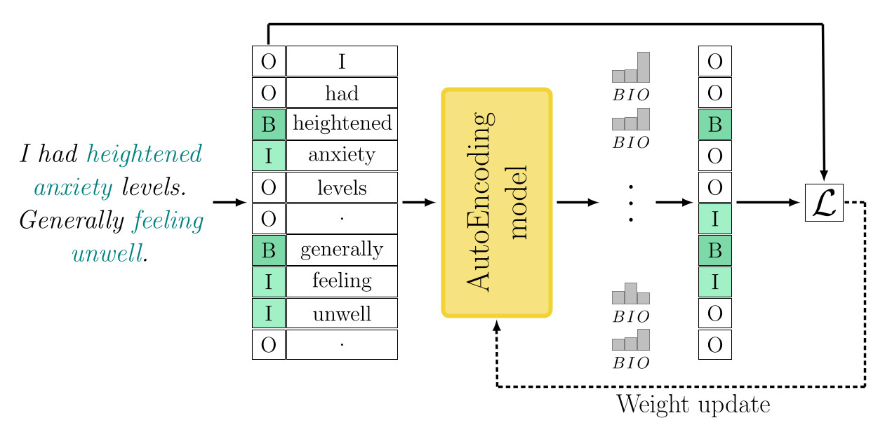
Figure 1: The ADE extraction pipeline for AutoEncoding models.

Following the literature on this task, we experiment and combine the AutoEncoding models with two additional processing layers: Conditional Random Fields (CRF) [23] and bidirectional LSTMs (BiLSTM) [22].

The AutoEncoding + CRF architecture combines the Transformer model with a CRF classifier. The BIO probability distribution generated by the Transformer model becomes the input of a CRF module, which produces another sequence of subword-level BIO labels. This step aims at denoising the sub-word output labels produced by the previous component.

The AutoEncoding + LSTM architecture combines the Transformer model with a BiLSTM. The embeddings generated by the Transformer model become the input of a one-layer BiLSTM that produces new embeddings of the same size. These new representations are then passed to a Linear Layer + Softmax, turning them into a probability distribution over the BIO labels.

3.2.2 AutoRegressive and Text-to-Text models

AutoRegressive and Text-to-Text models work similarly. Both kinds of models take a text as input and return a text as output. However, AutoRegressive models are composed of a stack of Transformers decoders, while Text-to-Text models use the entire decoder-decoder architecture of the original Transformer [17].

We train the models to produce as output the list of the ADEs present in the input text, separated by semicolons. This architecture and the training steps are shown in Figure 2.

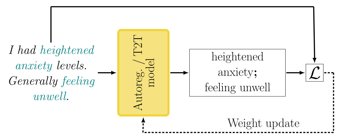
Figure 2: The ADE extraction pipeline for AutoRegressive and Text-to-Text models.

To evaluate the performance of the model, it is necessary to map its output back to the original text, however there is no guarantee that the strings produced by the model are exact substrings of the original text. Therefore, a simple postprocessing procedure is used to map the list of output ADEs to the input text. Let us consider the example in Figure 3. Each item in the semicolon-separated output can contain more than one word. If the item is a perfect sub-string of the input text, we consider it as single prediction. This is the case for “stomach ache”, which becomes span 1 after postprocessing. If the item is not a perfect sub-string if the input, we split it into shorter substrings that belong to the text and consider them as separate prediction. For example, the item “strong headache” gives origin to two predictions: spans 2 and 3. If part of the item cannot be found in the original text, such as “dizzy” in our examples, that part is completely discarded and does not generate a prediction.

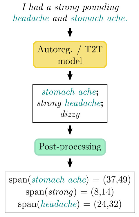
Figure 3: Example of the post-processing procedure used to map the string output of the AutoRegressive and Text-to-Text models to a list of ADE entities contained in the input text.

3.3 Transformer Variants

In this section, we briefly present the 19 Transformer-based model variants chosen for this survey, illustrating their main features. We start with all the models trained on general-domain texts only and then move to the variants that use in-domain knowledge, either medical or coming from social media data.

Notice that three of the in-domain variants were pre-trained from scratch (SciBERT, PubMedBERT, and BERTweet), meaning that they have a unique vocabulary tailored to their pre-training corpus and include specific embeddings for in-domain words.

Table 3 is a summary of the information about the version of all Transformer-based models used. The upper part of the Table lists general-domain variants (Section 3.3.1), while the lower part lists variants with in-domain knowledge (Section 3.3.2). The first column reports the model’s category (AutoEncoding, AutoRegressive or Text-to-Text). The column “From Scratch” marks which models were trained from scratch, as opposed to the ones which were initialized with another model’s weights (e.g., RoBERTa was trained from scratch while BioRoBERTa was initialized with RoBERTa’s weights and therefore shares part of its knowledge). The three columns under the name “Pre-training Domain” record the kind of documents which the models were pre-trained on: General domain knowledge (e.g., Wikipedia or BookCorpus), Medical domain (e.g., PubMed full-texts or health records), and Social domain (e.g., tweets or forum posts). For example, RoBERTa was pre-trained on General-domain documents only, while BioRoBERTa has both General-domain knowledge (derived from RoBERTa’s pre-training) and Medical-domain knowledge (derived from its own additional pre-training). Finally, the Table reports the model’s size in millions of parameters.

		From	Pre-training Domain			Model
Model Name	Category	Scratch	General	Medical	Social	Size
BERT	AutoEncoding	$\times$	$\times$			109M
DistilBERT	AutoEncoding		$\times$			66M
SpanBERT	AutoEncoding	$\times$	$\times$			108M
RoBERTa	AutoEncoding	$\times$	$\times$			124M
ELECTRA	AutoEncoding	$\times$	$\times$			109M
XLNet	AutoRegressive	$\times$	$\times$			118M
GPT-2	AutoRegressive	$\times$	$\times$			124M
T5	Text-to-Text	$\times$	$\times$			223M
PEGASUS	Text-to-Text	$\times$	$\times$			570M
BART	Text-to-Text	$\times$	$\times$			139M
BERTweet	AutoEncoding	$\times$			$\times$	354M
BioBERT	AutoEncoding		$\times$	$\times$		109M
BioClinicalBERT	AutoEncoding		$\times$	$\times$		108M
SciBERT	AutoEncoding	$\times$		$\times$		109M
PubMedBERT	AutoEncoding	$\times$		$\times$		108M
EnDR-BERT	AutoEncoding			$\times$	$\times$	177M
BioELECTRA	AutoEncoding	$\times$		$\times$		109M
BioRoBERTa	AutoEncoding		$\times$	$\times$		124M
SciFive	Text-to-Text		$\times$	$\times$		223M

Table 3: Information about the version of all the Transformer-based models used and their pre-training.

3.3.1 General-domain Variants

BERT [18], AutoEncoding. Standard model, pre-trained on general-domain texts (Wikipedia and BookCorpus) with two objectives: Masked Language Modeling (MLM) and Next Sentence Prediction (NPS). In MLM, a token in the input sentence is replaced with the MASK token and the goal of the model is to identify the original one. In NSP the model classifies the second input sentence as related or not to the first one. As mentioned in the related work, BERT achieved state-of-the-art results in several NLP tasks and worked as the foundation of many other pre-trained models.

DistilBERT [60], AutoEncoding. It is a distilled version of the original BERT model. A student network, with half the number of layers of BERT, is initialized with the weights of its BERT teacher, taking one layer out of two. The student model is then trained to replicate the output distribution of the teacher using three losses: Masked Language Modeling (MLM), distillation loss (CE), and cosine embedding loss (COS).

SpanBERT [61], AutoEncoding. A version of BERT that introduces an additional loss called Span Boundary Objective (SBO), alongside the traditional MLM loss used for BERT.
Let us consider a sentence $S=[w_{1},w_{2},\dots,w_{k}]$ and its sub-string $S_{m:n}=[w_{m},\dots,w_{n}]$. $w_{m-1}$ and $w_{n+1}$ are the boundaries of $S_{m:n}$ (the words immediately preceding and following it). We mask $S$ by replacing all the words in $S_{m:n}$ with the [MASK] token. SpanBERT reads the masked version of $S$ and returns an embedding for each word. The MLM loss measures if it is possible to reconstruct each original word $w_{i}\in S_{m:n}$ from the corresponding embedding. The SBO loss measures if it is possible to reconstruct each $w_{i}\in S_{m:n}$ using the embeddings of the boundary words $w_{m-1}$ and $w_{n+1}$. This kind of pre-training procedure makes its embeddings more appropriate for NER-like tasks.

RoBERTa [62], AutoEncoding. Starting from the assumption that BERT was under-trained, RoBERTa was developed changing some aspects of BERT’s pre-training phase. It dynamically changes the masking pattern: instead of using a static masking strategy, each training sample was duplicated 10 times, masking each sequence in 10 different ways. Additionally, RoBERTa is trained without the NSP objective, for more steps, with more data, bigger batches, and on longer text sequences. This model achieved state-of-the-art performances surpassing BERT on many general-domain NLP tasks.

ELECTRA [63], AutoEncoding. It is a pre-trained model where the MLM objective is replaced with the Replaced Token Detection task, in which the model learns to distinguish real input tokens from synthetically generated replacements. The network is trained as a discriminator that predicts for every token whether is original or a replacement. The role of the generator is usually covered by a small MLM model. In this way, the model gains knowledge from all input tokens instead of just the small masked-out subset. This approach keeps the performances close to the ones of BERT, while lowering the computational costs of training the model.

XLNet [64], AutoRegressive. It is a pre-trained model that tries to leverage the best of both AutoRegressive and AutoEncoding language modeling. Instead of using a fixed forward or backward factorization order, it maximizes the expected log-likelihood of a sequence with respect to all possible permutations. This objective is called Permutation Language Modeling. A difference with BERT is that this model does not rely on data corruption (e.g. token masking).

GPT-2 [29], AutoRegressive. It is a stack of transformer-decoders pre-trained with the simple objective of Next Word Prediction. As mentioned in the related work, it achieved state-of-the-art results on several text completion benchmarks.

T5 [30], Text-to-Text. It is an encoder-decoder model pre-trained on a multi-task mixture of unsupervised and supervised tasks. The are some small differences between T5 and the classical Transformer encoder-decoder. An example is the use of a normalization layer after each layer in both the encoder and decoder. The Span-based language masking objective is used during the pre-training phase, masking some randomly selected words in the input sentence and generating those words separated by the masking token $<$M$>$. The model has been trained using the C4 corpus [65].

PEGASUS [31], Text-to-Text. It is an encoder-decoder model pre-trained using a self-supervised objective (gap-sentence-objective) and created originally to improve the fine-tuning performance on abstractive summarization. In our case, the model is used in a text-generation setting and not specifically for a summarization task.

BART [66], Text-to-Text. It is a model pre-trained using two strategies: corrupting text by shuffling the original order of sentences and masking spans of text by replacing them with a mask token. It matches the performance of RoBERTa on several NLP benchmarks that require text comprehension, and is effective in text-generation tasks.

3.3.2 Domain-specific Variants

BERTweet [67], AutoEncoding. The model is trained from scratch using the same pre-training procedure of RoBERTa and a dataset containing 873M tweets. Some of them belong to the general Twitter Stream grabbed by the Archive Team, while others are related to the COVID-19 pandemic. We use the large version that allows us to input up to 512 tokens, analyzing the longer CADEC texts.

BioBERT [19], AutoEncoding. The model was pre-trained on PubMed abstracts starting from a BERT checkpoint. The authors of BioBERT provide different versions of the model, pre-trained on different corpora. We selected the version which seemed to have the greatest advantage on this task, according to the results by [19]. We chose BioBERT v1.1 (+PubMed), which outperformed other BioBERT v1.0 versions (including the ones trained on full texts) in NER tasks involving Diseases and Drugs. Preliminary experiments against BioBERT v.1.0 (+PubMed+PMC) confirmed this behavior on the datasets used in this work [56].

BioClinicalBERT [68], AutoEncoding. It was pre-trained on clinical texts from the MIMIC-III database [69], starting from a BioBERT checkpoint.

SciBERT [70], AutoEncoding. It was pre-trained from scratch on papers retrieved from Semantic Scholar [71] (82% of them belonging to the medical domain).

PubMedBERT [72], AutoEncoding. It was pre-trained from scratch on PubMed abstracts and full-text articles from PubMed Central. The vocabulary of PubMedBERT contains more in-domain medical words than any other model under consideration (as reported in their paper).

EnDR-BERT [20], AutoEncoding. The model was pre-trained on an English corpus of health-related comments [20] starting from a BERT base multilingual cased checkpoint.

BioRoBERTa [21], AutoEncoding. It was pre-trained from a RoBERTa-base checkpoint on biomedical full-text papers from S2ORC [73].

BioELECTRA [74], AutoEncoding. It was pre-trained from scratch on clinical texts from PubMed abstracts using the same architecture as ELECTRA.

SciFive [75], Text-to-Text. It is a domain-specific T5 model pre-trained on a large biomedical corpus of PubMed Abstracts and PMC articles, starting from a T5 checkpoint.

3.4 Metrics

Since the problem is framed as either multi-class token classification (BIO labels) or text generation, which eventually outputs a set of predicted entities, we use the standard evaluation metrics used by the ADE extraction community, which are entity-level relaxed F1 score, Precision and Recall. The following describes in detail how the metrics are calculated.

Given a set of gold (ground-truth) entities and a set of predicted entities, we can calculate the following values (see Figure 4): Correct ($Cor$), the number of entities which perfectly correspond to the gold ones; Missing ($Mis$) all gold entity not present in the predictions; Spurious ($Spu$) number of excess predicted entities; Partial/Incorrect ($Par$/$Inc$) the number of predicted entities which partially overlap a gold entity. In practice, one of the last two values is set to 0: $Par=0$ if we want to consider partially overlapping entities as incorrect, while $Inc=0$ if consider them as correct.

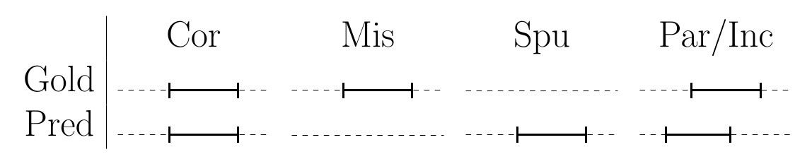
Figure 4: Visual representation of the intermediate metrics used to calculate Precision, Recall, and F1 score. The schema compares the presence of real annotations (Gold) and the predictions of the model (Pred).

Starting from these values, we define the main evaluation metrics used for this task, which are the Strict and Relaxed versions of the F1, Precision, and Recall scores [76], calculated at the entity level [77].

The Relaxed versions of the metrics, which allow for partial overlaps, are defined as follows:

$$Recall =\frac{Cor+(Par\times 0.5)}{Cor+Par+Inc+Mis}$$

$$Precision =\frac{Cor+(Par\times 0.5)}{Cor+Par+Inc+Spu}$$

$$F1 =\frac{2\times Precision\times Recall}{Precision+Recall}$$

The Strict Recall, Precision, and F1 score are calculated using the same formulas above, setting $Par=0$.

Relaxed and Strict metrics are highly correlated and follow the same trends. In this work, when commenting results we will always refer to the Relaxed metrics to keep the discussion concise and avoid repetitions. The Strict metrics are reported in B.

3.5 Feature Importance Analysis

Our objective is to analyze how some high-level features of the models correlate with their final performance (F1 score). For this reason, we characterize each model with the following six features:

1. Model Category: AutoEncoding (0), AutoRegressive (1), Text-to-Text (2);

2. Pre-training domain - General data: Yes, No;

3. Pre-training domain - Medical data: Yes, No;

4. Pre-training domain - Social data: Yes, No;

5. Pre-training from scratch: Yes, No;

6. Model Size (number of parameters): less than 100M (0), 100M–130M (1), over 130M (2).

The values of these features of all the models can be derived from Table 3. We encode Model Category using label encoding, as opposed to one-hot encoding. We prefer label encoding to one-hot encoding because it helps to better highlight and analyze the effect of the three values of this feature. Using one-hot encoding would split its contribution among three separate features and make it harder to see their interaction with the chosen technique. We verified that the ordering chosen to encode the features does not impact the results by permuting the values used to encode the Model Category and comparing all the results.

To explain the performance of the models starting from this set of high-level features, we employ Shapley values [25], a widely-used model interpretability technique. This technique assigns a positive or negative contribution to each value of all the input features, representing the impact that they have on the model’s output.

To calculate the Shapley values, we need to create a model that takes as input the six high-level features previously listed and outputs the F1 score of the Transformer variant. We choose a Random Forest model, as it is well-suited to work on low-dimensional data and it is also often used to perform these kinds of analyses. To generate a high number of input data to fit the Random Forest model, we use the results of all 30 runs of the previous experiments to calculate the performance of each Transformer-based variant. Therefore, we obtain 570 (30 $\times$ 19) samples containing the six high-level features and the F1 score of the models.

Figure 5 summarizes the process used to generate the Shapley values.

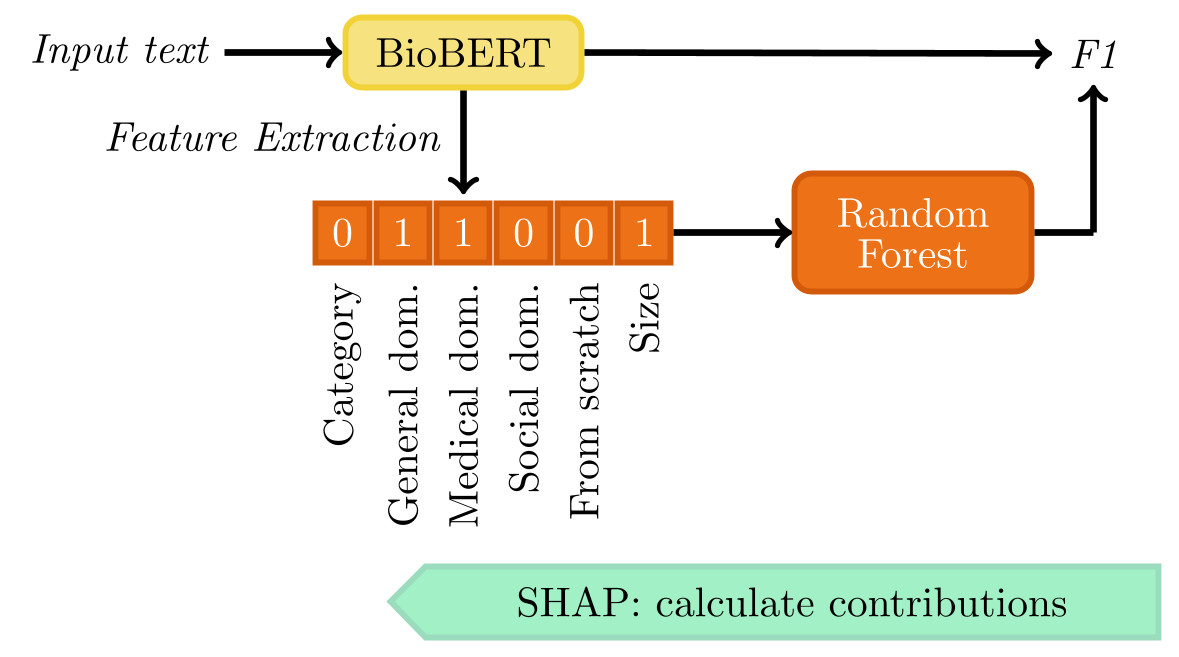
Figure 5: Process used to generate the Shapley values for the Transformer-based models.

After fitting the Random Forest, we can use the same set of data to calculate the attributions for each input feature and their values.

3.6 Training details

For all models, we performed hyperparameter tuning via grid-search. The models were evaluated on the training set and the best hyperparameters were chosen based on the highest relaxed F1 score.

We tested the following parameters:

• learning rate: $[5e{-5},5e{-6},1e{-3},1e{-4},1e{-5}]$

• dropout rate: from $0.15$ to $0.30$, increments of $0.05$

• batch size: $[8,16,32]$ for SMM4H, $[4,8]$ for CADEC

• training epochs: $1$ to $15$

The best hyperparameters selected for all the models are reported in A.

The input sequence length was fixed to $512$ for the CADEC dataset and $64$ for the SMM4H dataset.

AutoEncoding and Text-to-Text models were allowed to generate sequences with a maximum length of $40$ tokens for CADEC and $20$ tokens for SMM4H, based on the expected output sequence length in the training set.

During the final evaluation, all the models were tested on the test set, after being trained with the best hyperparameters on the concatenation of the training set and the validation set. The evaluation was repeated thirty times with different random seeds. We report the average of the results over the thirty runs.

Both training and testing have been performed using an Nvidia GeForce 3090. The average training time for a single epoch is 40 seconds on SMM4H and 90 seconds on CADEC for the base models. The training time increases slightly for the architectures using the additional LSTM layer and doubles for the architectures using the CRF layer.

4 Results and Discussion

First, we start by analyzing the performance of the base Transformer-based architectures without additional processing modules. We discuss the results of all the models on the two datasets, taking into account the Shapley values to discover patterns in the performances of the models. Secondly, we discuss the effects of using the additional CRF and LSTM modules, and how they have different effects on the two datasets.

4.1 Base Models Performance

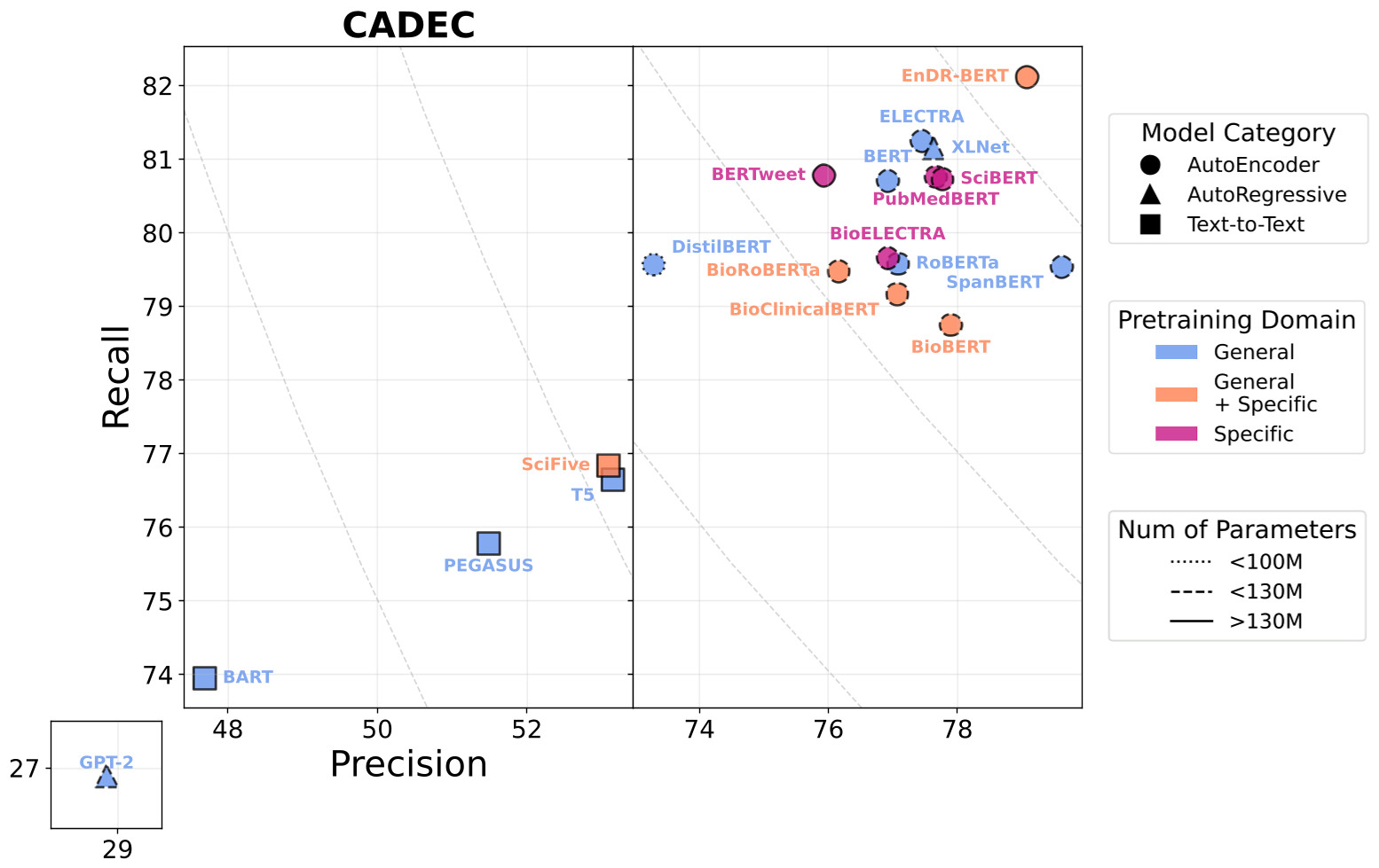
Figure 6: Precision and Recall of all the base models (with no additional modules) on the CADEC dataset.

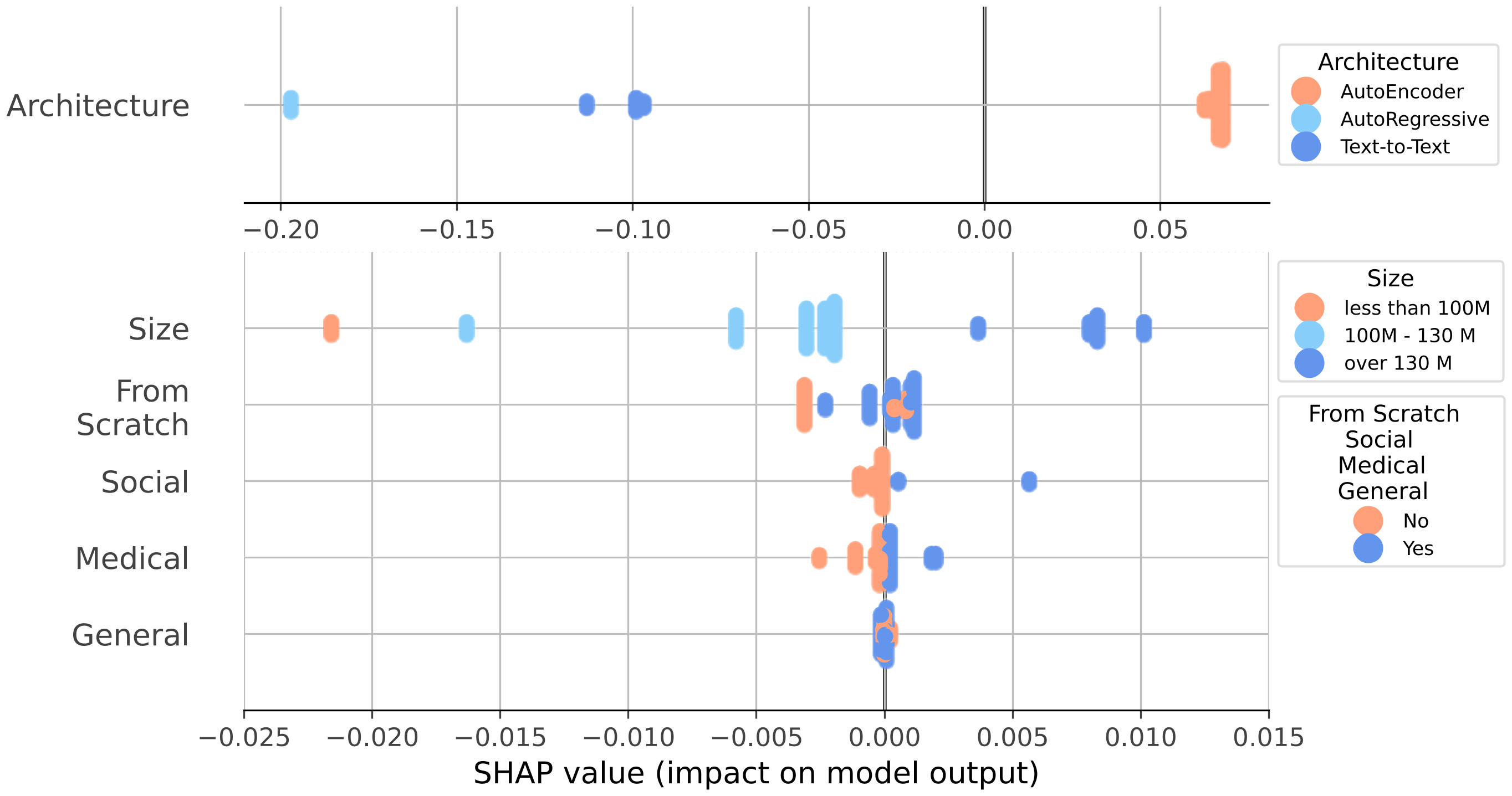
Figure 7: Shapley values calculated on the CADEC dataset.

We start by analyzing the performance of all the base models (without additional LSTM/CRF modules) on the CADEC dataset. We report the Precision and Recall of the models in Figure 6, while Figure 7 contains the results of the feature importance analysis performed with the Shapley values.

In Figure 6, different shapes represent different models categories: $\mathbin{\scalerel*{\bigcirc}{t}}$ for AutoEncoding models, $\triangle$ for AutoRegressive models, and $\square$ for Text-to-Text models. The colors show the domain of the training data of the model: general in blue    , specialized (medical or social) in violet    , mixed general and specialized in coral    . The linestyle of the markers shows the size of the model: dotted if the model has less than 100M parameters, dashed if the model has between 100M and 130M parameters, and solid if it is larger than 130M parameters. The dashed gray lines on the plot are iso-F1 curves, showing points of equal F1-score.

As regards Figure 7, each row represents one of the features used by the Random Forest to predict the F1 score of the models. Each point in a row is a sample, and its color represents the input value of its feature. For example, considering the feature Architecture, coral points are AutoEncoding models, light-blue points are AutoRegressive models, and blue points are Text-to-Text models. The x-coordinate represents SHAP values, which are positive if the feature contributes to a higher F1 score, and negative if it decreases it. The features are arranged in order of importance, from top to bottom, based on the magnitude of the SHAP values (i.e., their impact on the F1 score).

Looking at Figure 6, we can clearly distinguish three clusters of models: the AutoEncoding models $\mathbin{\scalerel*{\bigcirc}{t}}$ in the top right (together with XLNet), which reach the highest performance; the Text-to-Text models $\square$, which have a considerably lower Precision; GPT-2 (one of the AutoRegressive models $\triangle$), which has the worst performance overall and is clearly separated from the other Transformer variants. This is confirmed by the Shapley values (Figure 7), which show that Architecture is the most impactful feature, and its three values (coral, light-blue and blue) have different impacts (negative or positive) on the expected F1 score. All the models based on text generation (except XLNet) have a low Recall (lower than 77%), and even lower Precision (lower than 53%), which clearly separates them from the AutoEncoding models. The low Recall is probably caused by the high number of ADEs that need to be generated for the CADEC dataset, as the Text-to-Text models seem to struggle to generate long sequences of ADEs.

If we focus on the cluster of AutoEncoding models, we can see that the best-performing model overall is EnDR-BERT, which is also the largest AutoEncoding model (solid outline). Conversely, the worst model of the cluster is DistilBERT, which is the smallest model (dotted outline). Smaller models generally lead to a lower F1 score, which is also attested by the Shapley values (Size is the second most impactful feature on the performance of the models).

The third most impactful feature on Figure 7 is From scratch: models which are not pre-trained from scratch have generally a lower performance compared with the ones pre-trained from scratch. These models correspond to the five mixed-domain ones     and DistilBERT. We can see that this is mostly true for the three AutoEncoding models BioRoBERTa, BioClinicalBERT, and BioBERT. EnDR-BERT and SciFive counter the relative drop in performance thanks to their large size.

Another interesting observation from the Shapley values, is that pre-training on Social or Medical data has a positive impact on the model’s performance (blue points have positive SHAP values). These models correspond to the in-domain models     in Figure 6, where they are shown to achieve the same performance as models trained on general-domain data    . The positive contribution seems to be too small to have an effect on this plot, where it is overshadowed by the effects of the other model characteristics.

Overall, the model that achieves the highest Precision on CADEC is SpanBERT (general-domain    ), while the one with the highest Recall and F1 score is EnDR-BERT. Since the texts and ADE mentions present in CADEC are particularly long (see Character Count in Table 2), SpanBERT probably has an advantage over other models thanks to its span-based pre-training.

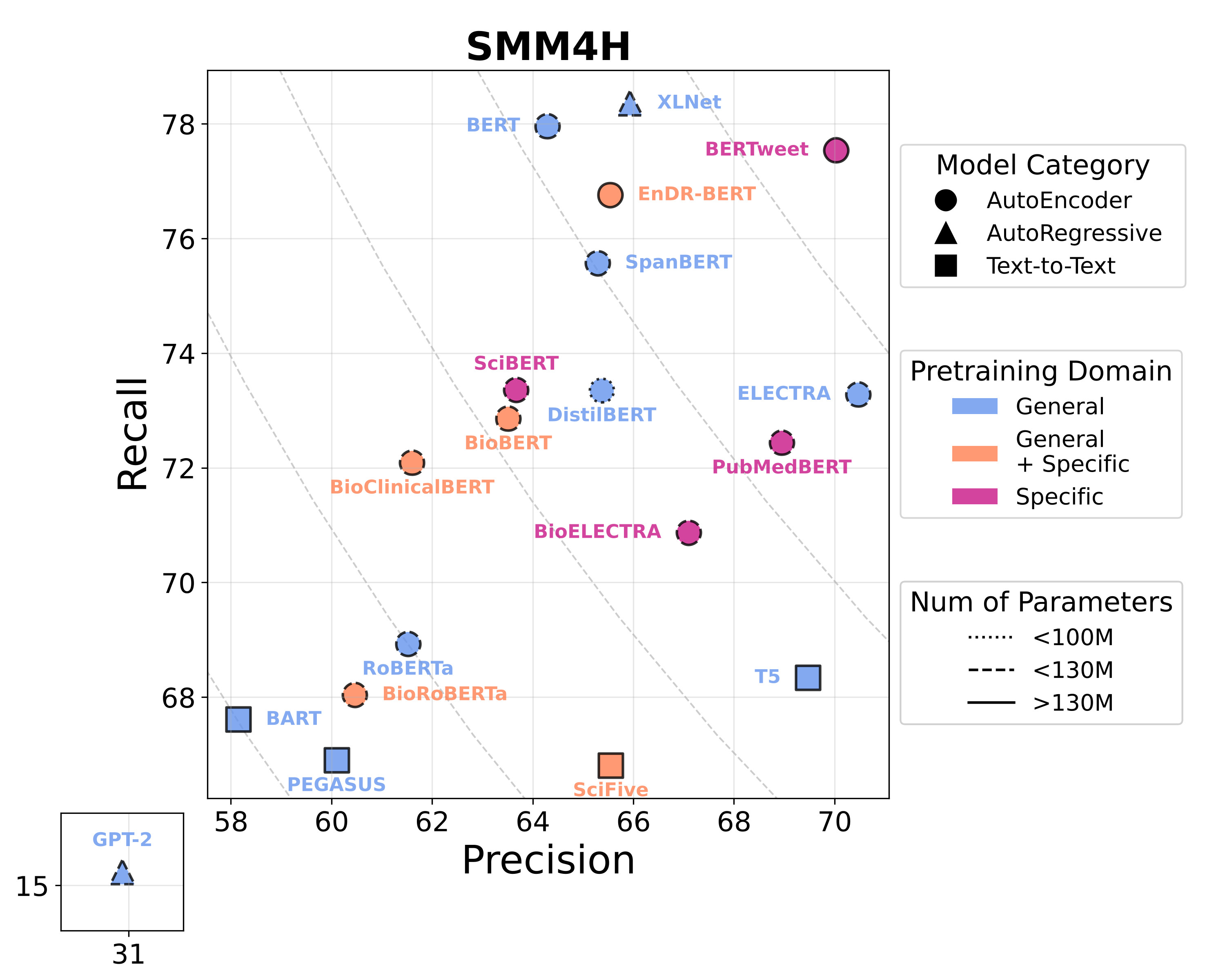
Figure 8: Precision and Recall of all the base models (with no additional modules) on the SMM4H dataset.

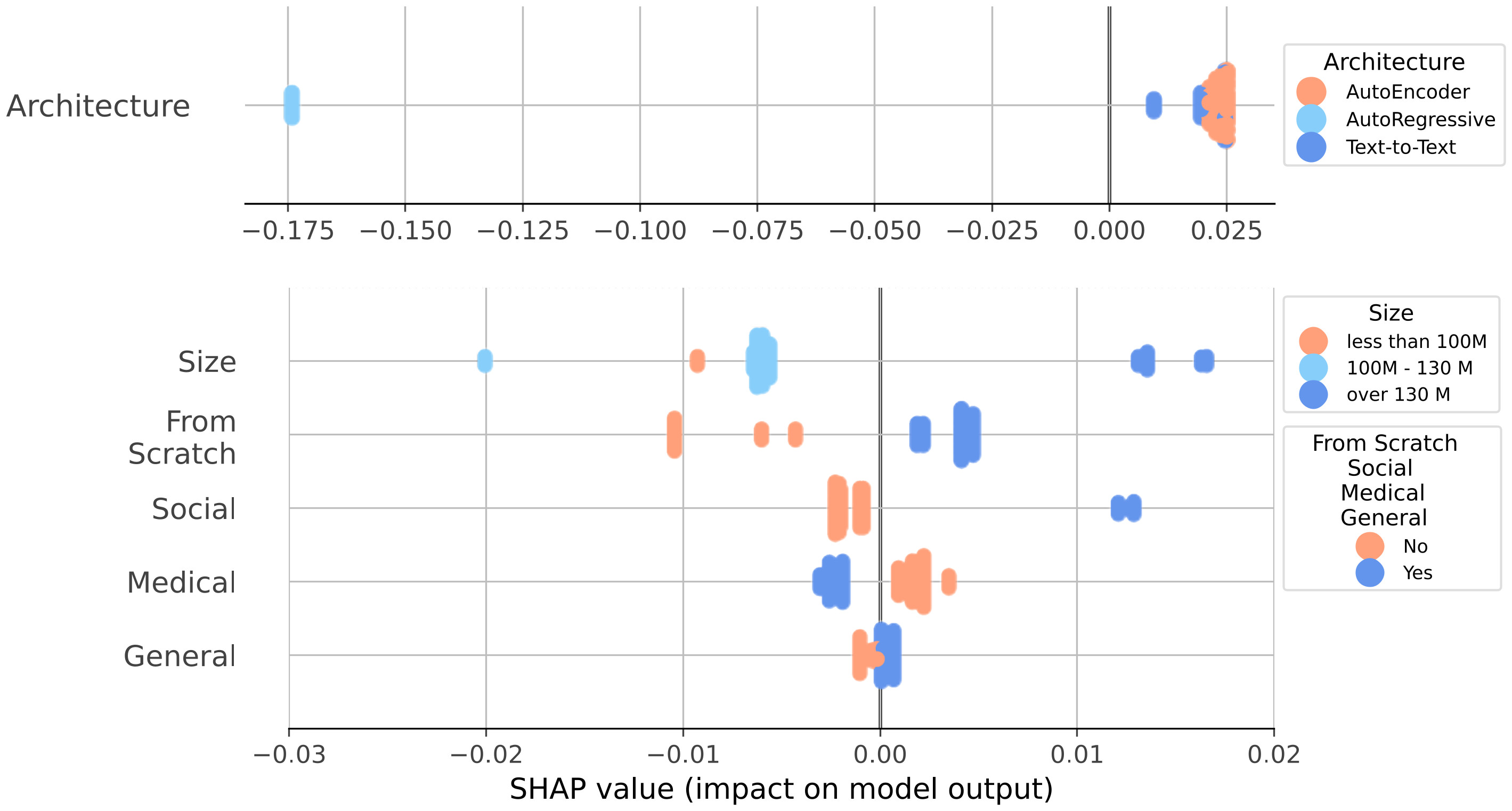
Figure 9: Shapley values calculated on the SMM4H dataset.

Figure 8 and 9 report the same information as the previous ones, but for the SMM4H dataset. The order of the most impactful features according to the Shapley values is the same for the two datasets.

Differently from CADEC, there are two noticeable clusters in Figure 8: GPT-2 and all the other Transformer-based variants. Similarly to CADEC, the Text-to-Text models $\square$ have a lower Recall than most of the AutoEncoding models $\mathbin{\scalerel*{\bigcirc}{t}}$. However, on the SMM4H dataset their Recall is closer to the other AutoEncoding models (RoBERTa and BioRoBERTa), and their Precision is also on-par with most of the other ones. For these reasons, they do not create a separate performance cluster as happened in CADEC. This is further confirmed by the Shapley values in Figure 9: the feature Architecture presents only two clusters (AutoRegressive vs others), and both AutoEncoding (coral) and Text-to-Text (blue) samples contribute to an increase in F1 score.

The model Size is still the second most impactful SHAP feature, but its effect on the Precision-Recall plot is more difficult to observe.

In sharp contrast with CADEC, the use of Medical domain pre-training leads to a lower performance, while General domain data slightly increases it. Social data pre-training also has a sharp positive impact. This indicates that medical in-domain knowledge leads to no advantage when dealing with highly informal texts, such as tweets. Indeed, most of the models that reach the best performance in terms of Precision, Recall, or F1-score are trained on general-domain data only (e.g., XLNet, BERT, and ELECTRA). The only cases in which in-domain knowledge brings an advantage are BERTweet and EnDR-BERT, which are trained on social media texts (tweets and forum posts), highlighting that, in this case, social media pre-training is more valuable than medical knowledge.

Finally, the effect of training a model From Scratch is more noticeable on SMM4H, where it leads to a small increase in performance. Models that are not trained from scratch correspond to the mixed-domain models     in Figure 8, and this decreases their F1 score according to the Shapley values. This loss in performance is probably connected to the fact that most mixed-domain models include medical knowledge, which is not beneficial on the SMM4H dataset.

To summarize, for both datasets: text-generation models (AutoRegressive and Text-to-Text) lead to the lowest performance; larger models tend to have higher performance; using models trained from scratch (regardless of their domain) is beneficial; knowledge of social media language is highly beneficial.

The main difference between the two datasets is that models pre-trained on medical data have lower performance on SMM4H, due to the large gap in textual style.

4.2 Error Analysis

Given the large number of analyzed models, it is challenging to perform an in-depth error analysis and compare the kind of errors produced by the various base models. However, we performed a qualitative analysis of the output of the models as follows. We fixed one of the thirty random seeds and gathered all the predictions of the 19 base models. We divided the predictions into the following sets: Correct, Partial, Missing and Spurious (see Section 3.4 for the definitions). We then compared these sets of predictions for all the models, creating rankings (ordering the predictions according to how many models classified it as Correct/Missing/Spurious) and grouping the predictions by topic (e.g., sleep disorders or weight change). The following trends emerged:

• Spurious predictions on CADEC and SMM4H. For both of the datasets, 80% of the Spurious predictions are unique (predicted only once and by less than three models out of 19). The spurious entities which are wrongly extracted/generated by all the models are short one-word entities, which are diseases (or symptoms of a disease, such as “headaches”), but denote real ADE mentions in other samples.

• AutoRegressive and Text-to-Text models on CADEC. A large amount of the gold entities belongs to the Missing set for all the models and are never predicted (neither as Correct nor as Partial). The entities which are consistently Missing for all the text-generation models are composed of multiple words (e.g., “affected my balance”, “blood pressure elevated”, “altered my heart function”) and they are often very technical (e.g., “peripheral neuropathy”, “gastrointestinal cramping”, “rheumatoid arthrtitis”).
  On the other hand, the entities which are predicted correctly by all the text-generation models (Correct and Partial) are short, one-word entities which are present in multiple samples (e.g., “constipation”, “diarrhea”, “fatigue”, “insomnia”).

• AutoEncoding models on CADEC. The proportion of Missing entities for the AutoEncoding models is significantly smaller, as confirmed by their higher Recall. The entities which are missed by all the models are extremely short ones (e.g., “sick”, “pain”, “gas”), which are difficult to contextualize, and extremely long ones (e.g., “will never get back the full use of my arms or legs”). In general, all models struggle to identify ADE with long character counts.

• All models on SMM4H. The overall number of Missing entities is low. The ones which are shared among all the models are extremely short, and some of them are hashtags (e.g., “#nosleepp”, “#wideawake”). The Missing entities which are common for all the models trained on medical domain only are short, colloquial terms such as “puking”, “out of it” and “passing out”.

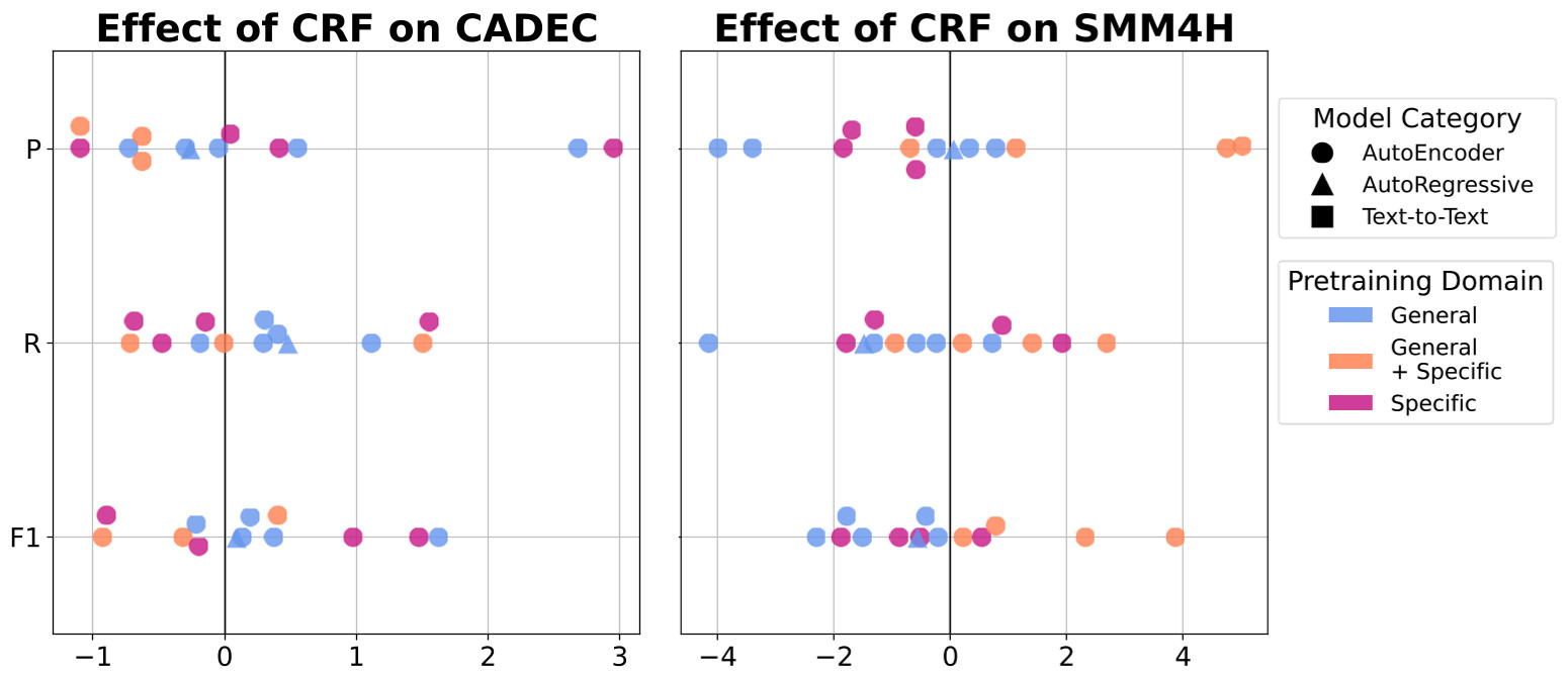
Figure 10: Effect of the CRF module on Precision and Recall.

4.3 Effect of the CRF

Figure 10 shows the effect that using the additional CRF module has on the AutoEncoding model and XLNet. The plots report the difference between the metric achieved by the model with the CRF module and the one without. Positive values indicate an advantage in using the additional module, while negative values mean it decreases the base performance of the model.

Looking at the results on the CADEC dataset, we observe that the CRF module generally has a positive impact on the Recall of the models and a mixed impact on the Precision. It leads to a gain of up to 3 points in Precision and up to 1.5 points in Recall, leading to an overall increase in F1-score too. There seems to be no pattern that relates the pre-training domain with the effect of the CRF module.

On the SMM4H dataset, the CRF module seems to have different effects based on the pre-training domain of the models. It leads to a decrease in Precision for models with specific or general-domain knowledge (       ), with a subsequent loss in F1-score. On the contrary, mixed-domain models (   ) experience a gain in Precision (up to 4 points) and in Recall, with an overall increase in F1-score.

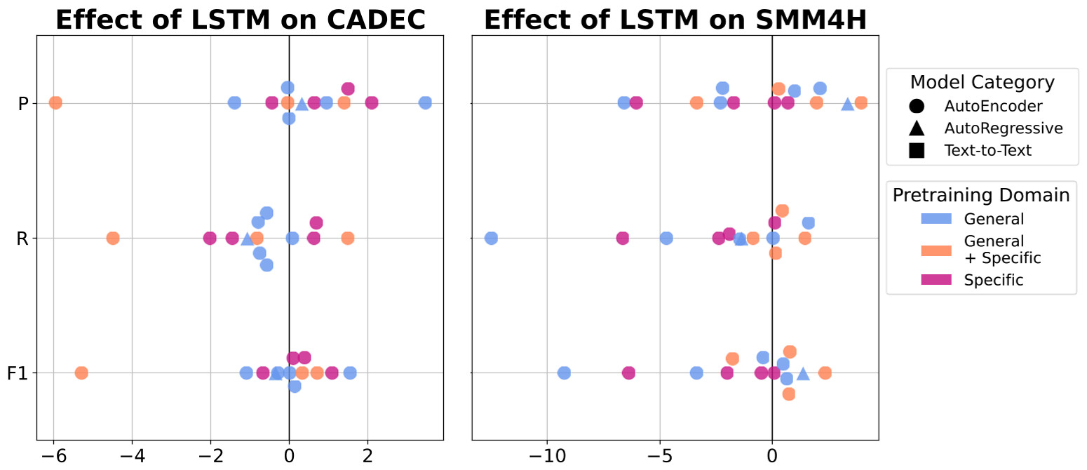
Figure 11: Effect of the LSTM module on Precision and Recall.

4.4 Effect of the LSTM

In Figure 11 we report the results for the LSTM module using the same format of Figure 10.

On the CADEC dataset, the LSTM generally increases the Precision of the models (up to 2.5 points) and has a small (mostly negative) impact on the Recall, which is more frequent for general-domain (   ) models. The overall effect is generally an increase in F1-score.

The effect of the LSTM on the SMM4H dataset seems to show no regularities: the Precision increases or decreases with no definite pattern, almost all the models experience a drop in Recall (up to 12.5 points). The overall effect on the F1-score is negative.

The LSTM seems to have a similar effect on both datasets, therefore it could be reasonable to use it in cases where we are interested in increasing the Precision of the base model.

4.5 Take-home Messages

To summarize the results of all the previous experiments, we observed that:

• AutoEncoding models are the best choice of model to deal with this task, while models based on text generation (AutoRegressive and Text-to-Text) do not have good performances on long texts or texts that contain a high number of ADEs;

• when all other features are the same, bigger models have the highest performance on both formal and informal texts;

• pre-training on social media texts leads to a consistent increase in performance on both datasets, while medical pre-training is only effective when working with social media texts that have a more formal language (in this case the forum posts from CADEC);

• the use of additional modules needs to be evaluated on a case-by-case basis. On the whole, the CRF module has a positive impact on the Recall of the models when used in formal texts, and positive effects on Precision for mixed-domain models in informal texts. On the other hand, the LSTM tends to increase the Precision of the models in formal texts but has negative effects on most of the metrics in informal texts.

5 Conclusions

In this paper, we performed a systematic analysis of 19 transformer-based models for ADE extraction on informal texts. We compared their performance on two datasets with different textual styles, and correlated it with the following model features: category (AutoEncoding, AutoRegressive, Text-to-Text), pre-training domain, training from scratch, and model size in number of parameters. We used feature importance techniques to correlate each of these characteristics to the performance of the models. Furthermore, we analyzed the impact of commonly-used additional processing layers (CRF and LSTM) on the performance of the models. To conclude our analyses, we presented a list of take-home messages that can be derived from the experimental data.

Since the code we used for these analyses is publicly available, it will be possible to adapt it and use it for other tasks. In particular, future researchers will be able to use it to test different kinds of models comparing their features and performances on other tasks and domains.

In the future, we plan to expand our analyses to other tasks in the medical domain. This will help building a more solid understanding of which model characteristics are more effective for each task, especially in the new field of digital pharmacovigilance on social media texts.

Appendix A Further details on the models

Table 4 reports the unique identifiers of all the models in the HuggingFace library for reproducibility.

Name	Model name in the Transformers library
BERT	bert-base-uncased
DistilBERT	distilbert-base-uncased
SpanBERT	SpanBERT/spanbert-base-cased
RoBERTa	roberta-base
ELECTRA	google/electra-base-discriminator
XLNet	xlnet-base-cased
GPT-2	gpt2
T5	t5-base
PEGASUS	google/pegasus-xsum
BART	facebook/bart-base
BERTweet	vinai/bertweet-large
BioBERT	monologg/biobert_v1.1_pubmed
BioClinicalBERT	emilyalsentzer/Bio_ClinicalBERT
SciBERT	allenai/scibert_scivocab_cased
PubMedBERT	microsoft/BiomedNLP-PubMedBERT-base-uncased-abstract-fulltext
EnDR-BERT	cimm-kzn/endr-bert
BioELECTRA	kamalkraj/bioelectra-base-discriminator-pubmed
BioRoBERTa	allenai/biomed_roberta_base
SciFive	razent/SciFive-base-Pubmed

Table 4: Unique identifiers of the models in the Huggingface Transformer library.

Table 5 contains the best hyperparameters used for all architectures on SMM4H and CADEC, respectively.

	CADEC				SMM4H20
Model Name	lr	dropout	epoch	batch_size	lr	dropout	epoch	batch_size
BERT	1e-4	0.25	6	4	5e-5	0.25	10	16
BERTweet	5e-5	0.3	8	4	5e-5	0.15	7	16
BioBERT	1e-4	0.2	7	8	5e-5	0.2	5	16
BioClinicalBERT	5e-5	0.2	8	4	5e-5	0.15	3	8
BioELECTRA	5e-5	0.2	9	8	1e-4	0.2	4	8
BioRoBERTa	1e-4	0.25	15	8	5e-5	0.15	7	16
DistilBERT	5e-5	0.3	7	8	1e-4	0.3	4	8
ELECTRA	5e-5	0.15	8	8	5e-5	0.15	7	32
EnDR-BERT	5e-5	0.3	14	4	5e-5	0.15	5	32
PubMedBERT	5e-5	0.3	10	4	5e-5	0.2	10	16
RoBERTa	5e-5	0.15	10	8	5e-5	0.15	7	8
SciBERT	5e-5	0.3	13	4	5e-5	0.3	13	8
SpanBERT	5e-5	0.15	10	4	5e-5	0.15	8	8
XLNet	5e-5	0.15	7	4	5e-5	0.2	15	32
T5	2-e4	0.15	9	4	5e-5	0.15	10	8
GPT-2	1-e3	0.15	6	8	5e-5	0.15	4	32
BART	5-e5	0.15	10	32	6e-5	0.15	10	16
PEGASUS	2-e4	0.15	5	4	5e-5	0.15	8	8
SciFive	6-e5	0.15	12	4	1e-4	0.15	11	8
BERT +CRF	1e-4	0.3	9	4	1e-4	0.3	7	16
BERTweet +CRF	5e-5	0.25	11	4	5e-5	0.15	6	32
BioBERT +CRF	5e-5	0.25	7	8	1e-4	0.2	6	8
BioClinicalBERT +CRF	5e-5	0.25	7	4	1e-4	0.2	5	16
BioELECTRA +CRF	5e-5	0.3	15	4	1e-4	0.15	5	16
BioRoBERTa +CRF	5e-5	0.25	9	4	5e-5	0.15	8	16
DistilBERT +CRF	1e-4	0.3	8	8	1e-4	0.25	5	8
ELECTRA +CRF	5e-5	0.25	10	4	1e-4	0.25	7	16
EnDR-BERT +CRF	1e-4	0.25	8	8	5e-5	0.15	4	16
PubMedBERT +CRF	1e-4	0.3	14	8	5e-5	0.2	8	8
RoBERTa +CRF	5e-5	0.15	8	4	5e-5	0.2	10	8
SciBERT +CRF	5e-5	0.2	6	4	1e-4	0.2	6	32
SpanBERT +CRF	5e-5	0.15	9	8	5e-5	0.15	7	8
XLNet +CRF	5e-5	0.25	12	4	5e-5	0.15	7	16
BERT +LSTM	5e-5	0.2	7	4	5e-5	0.25	7	8
BERTweet +LSTM	5e-5	0.15	8	4	5e-5	0.15	15	32
BioBERT +LSTM	5e-5	0.2	8	4	5e-5	0.25	7	8
BioClinicalBERT +LSTM	1e-4	0.3	9	4	5e-5	0.25	9	16
BioELECTRA +LSTM	5e-5	0.25	12	4	5e-5	0.2	8	8
BioRoBERTa +LSTM	5e-5	0.15	9	4	5e-5	0.25	14	8
DistilBERT +LSTM	1e-4	0.2	6	4	1e-4	0.2	6	16
ELECTRA +LSTM	5e-5	0.2	6	4	5e-5	0.2	11	32
EnDR-BERT +LSTM	1e-4	0.3	9	8	5e-5	0.15	5	8
PubMedBERT +LSTM	1e-4	0.15	8	8	5e-5	0.15	8	16
RoBERTa +LSTM	5e-5	0.15	10	4	5e-5	0.2	14	16
SciBERT +LSTM	5e-5	0.3	12	4	5e-5	0.25	14	32
SpanBERT +LSTM	5e-5	0.15	8	8	5e-5	0.2	10	8
XLNet +LSTM	5e-5	0.15	9	4	5e-5	0.15	12	32

Table 5: Best hyperparameters for all models.

Appendix B Detailed metrics of all the models

The following tables report the Strict and Relaxed evaluation metrics for all the models used in the paper. Tables 6–8 report the results on SMM4H. Tables 9–11 report the results on CADEC.

	Relaxed			Strict
	F1	P	R	F1	P	R
BERT	70.43 $\pm$ 0.22	64.29 $\pm$ 1.53	77.96 $\pm$ 1.79	61.99 $\pm$ 0.90	56.65 $\pm$ 1.44	68.52 $\pm$ 2.11
DistilBERT	69.09 $\pm$ 1.36	65.37 $\pm$ 2.62	73.35 $\pm$ 1.27	60.70 $\pm$ 1.41	57.43 $\pm$ 2.39	64.44 $\pm$ 1.48
SpanBERT	70.04 $\pm$ 1.01	65.29 $\pm$ 1.76	75.57 $\pm$ 0.10	62.59 $\pm$ 1.39	57.84 $\pm$ 2.83	68.33 $\pm$ 0.85
RoBERTa	64.97 $\pm$ 1.08	61.52 $\pm$ 1.95	68.93 $\pm$ 2.14	56.12 $\pm$ 1.23	53.25 $\pm$ 1.99	59.41 $\pm$ 1.86
ELECTRA	71.81 $\pm$ 1.51	70.47 $\pm$ 1.89	73.28 $\pm$ 2.60	63.46 $\pm$ 1.91	62.45 $\pm$ 1.73	64.58 $\pm$ 3.09
XLNet	71.55 $\pm$ 0.52	65.93 $\pm$ 1.79	78.36 $\pm$ 2.37	62.89 $\pm$ 0.88	57.80 $\pm$ 1.23	69.07 $\pm$ 2.71
GPT-2	20.15 $\pm$ 2.74	30.83 $\pm$ 2.58	15.19 $\pm$ 2.85	11.73 $\pm$ 4.74	17.16 $\pm$ 5.87	08.97 $\pm$ 3.82
T5	68.90 $\pm$ 1.08	69.47 $\pm$ 1.60	68.34 $\pm$ 0.77	61.90 $\pm$ 1.08	62.42 $\pm$ 1.58	61.40 $\pm$ 0.72
PEGASUS	63.31 $\pm$ 0.84	60.10 $\pm$ 1.38	66.90 $\pm$ 0.76	55.90 $\pm$ 1.05	53.07 $\pm$ 1.47	59.07 $\pm$ 0.89
BART	62.44 $\pm$ 1.81	58.15 $\pm$ 3.87	67.61 $\pm$ 1.42	54.35 $\pm$ 1.85	50.62 $\pm$ 3.61	58.85 $\pm$ 1.11
BERTweet	73.57 $\pm$ 0.72	70.03 $\pm$ 1.07	77.54 $\pm$ 2.17	64.44 $\pm$ 1.56	61.34 $\pm$ 1.38	67.93 $\pm$ 2.69
BioBERT	67.83 $\pm$ 0.72	63.51 $\pm$ 1.56	72.86 $\pm$ 2.03	59.62 $\pm$ 1.56	55.81 $\pm$ 1.47	64.06 $\pm$ 2.81
BioClinicalBERT	66.42 $\pm$ 1.19	61.60 $\pm$ 1.73	72.09 $\pm$ 1.16	57.52 $\pm$ 1.20	53.40 $\pm$ 1.62	62.36 $\pm$ 1.26
SciBERT	68.14 $\pm$ 0.72	63.67 $\pm$ 1.96	73.36 $\pm$ 1.40	59.77 $\pm$ 0.94	55.91 $\pm$ 1.87	64.28 $\pm$ 1.34
PubMedBERT	70.63 $\pm$ 0.91	68.95 $\pm$ 1.13	72.44 $\pm$ 1.82	63.00 $\pm$ 1.18	61.90 $\pm$ 2.00	64.23 $\pm$ 2.15
EnDR-BERT	70.64 $\pm$ 1.21	65.54 $\pm$ 2.88	76.76 $\pm$ 1.38	62.36 $\pm$ 1.33	57.39 $\pm$ 2.26	68.37 $\pm$ 1.32
BioRoBERTa	64.01 $\pm$ 0.83	60.46 $\pm$ 0.71	68.04 $\pm$ 1.90	54.68 $\pm$ 1.20	50.85 $\pm$ 1.55	59.24 $\pm$ 2.60
BioELECTRA	68.93 $\pm$ 1.40	67.10 $\pm$ 1.54	70.87 $\pm$ 1.75	61.62 $\pm$ 1.78	59.99 $\pm$ 1.84	63.36 $\pm$ 2.04
SciFive	66.16 $\pm$ 1.09	65.55 $\pm$ 2.01	66.81 $\pm$ 1.02	59.75 $\pm$ 1.14	59.20 $\pm$ 2.05	60.34 $\pm$ 0.74

Table 6: Metrics of all the base models on SMM4H.

	Relaxed			Strict
	F1	P	R	F1	P	R
BERT	70.19 $\pm$ 0.42	64.03 $\pm$ 1.07	77.69 $\pm$ 1.10	62.14 $\pm$ 0.62	56.69 $\pm$ 0.90	68.79 $\pm$ 1.34
DistilBERT	68.64 $\pm$ 0.52	65.67 $\pm$ 1.82	72.01 $\pm$ 1.99	59.19 $\pm$ 1.09	57.14 $\pm$ 1.41	61.42 $\pm$ 1.29
SpanBERT	68.50 $\pm$ 2.99	66.04 $\pm$ 3.68	71.39 $\pm$ 4.50	60.25 $\pm$ 3.71	58.10 $\pm$ 4.21	62.79 $\pm$ 4.73
RoBERTa	62.64 $\pm$ 3.46	58.09 $\pm$ 5.54	68.32 $\pm$ 0.99	53.38 $\pm$ 4.78	49.46 $\pm$ 6.12	58.21 $\pm$ 2.76
ELECTRA	70.00 $\pm$ 1.61	66.45 $\pm$ 1.43	73.97 $\pm$ 1.82	61.32 $\pm$ 2.68	56.25 $\pm$ 3.82	67.49 $\pm$ 0.97
XLNet	70.97 $\pm$ 1.16	65.97 $\pm$ 1.85	76.86 $\pm$ 1.60	61.17 $\pm$ 1.55	56.81 $\pm$ 2.03	66.31 $\pm$ 1.80
BERTweet	74.08 $\pm$ 0.96	69.41 $\pm$ 1.45	79.43 $\pm$ 0.64	65.24 $\pm$ 1.19	61.13 $\pm$ 1.31	69.96 $\pm$ 1.40
BioBERT	70.12 $\pm$ 1.81	68.50 $\pm$ 1.29	71.88 $\pm$ 3.10	63.25 $\pm$ 2.94	61.77 $\pm$ 2.13	64.86 $\pm$ 4.10
BioClinicalBERT	70.26 $\pm$ 1.24	66.32 $\pm$ 1.67	74.75 $\pm$ 2.02	62.25 $\pm$ 2.33	58.35 $\pm$ 2.70	66.78 $\pm$ 2.77
SciBERT	67.23 $\pm$ 0.92	63.04 $\pm$ 1.08	72.03 $\pm$ 1.02	58.62 $\pm$ 1.04	54.96 $\pm$ 1.16	62.81 $\pm$ 1.09
PubMedBERT	70.08 $\pm$ 1.14	67.23 $\pm$ 2.14	73.30 $\pm$ 2.51	62.65 $\pm$ 1.36	60.20 $\pm$ 2.19	65.42 $\pm$ 2.38
EnDR-BERT	71.39 $\pm$ 1.09	66.64 $\pm$ 1.93	76.94 $\pm$ 1.67	63.44 $\pm$ 1.18	58.88 $\pm$ 2.35	68.88 $\pm$ 1.62
BioRoBERTa	64.20 $\pm$ 1.09	59.74 $\pm$ 0.64	69.42 $\pm$ 2.32	54.94 $\pm$ 0.86	50.90 $\pm$ 0.58	59.73 $\pm$ 2.16
BioELECTRA	67.02 $\pm$ 1.91	65.23 $\pm$ 2.13	69.05 $\pm$ 3.49	59.02 $\pm$ 1.90	58.20 $\pm$ 2.76	59.93 $\pm$ 1.96

Table 7: Metrics of the AutoEncoding models with CRF module on SMM4H.

	Relaxed			Strict
	F1	P	R	F1	P	R
BERT	71.03 $\pm$ 1.12	65.24 $\pm$ 1.12	77.95 $\pm$ 1.56	62.94 $\pm$ 1.39	57.89 $\pm$ 1.29	69.00 $\pm$ 2.44
DistilBERT	69.53 $\pm$ 0.81	67.45 $\pm$ 2.42	71.86 $\pm$ 1.30	60.38 $\pm$ 1.30	58.58 $\pm$ 2.65	62.39 $\pm$ 0.90
SpanBERT	60.75 $\pm$ 0.07	58.66 $\pm$ 1.26	63.04 $\pm$ 1.31	50.06 $\pm$ 0.68	47.18 $\pm$ 0.82	53.33 $\pm$ 0.49
RoBERTa	61.56 $\pm$ 3.87	59.17 $\pm$ 4.12	64.18 $\pm$ 3.72	50.23 $\pm$ 6.63	48.30 $\pm$ 6.64	52.35 $\pm$ 6.67
ELECTRA	71.36 $\pm$ 1.49	68.22 $\pm$ 2.20	74.85 $\pm$ 1.38	62.64 $\pm$ 1.51	59.89 $\pm$ 2.22	65.69 $\pm$ 1.10
XLNet	72.90 $\pm$ 1.28	69.26 $\pm$ 1.50	76.97 $\pm$ 1.46	64.35 $\pm$ 1.90	61.14 $\pm$ 2.08	67.94 $\pm$ 1.90
BERTweet	73.04 $\pm$ 1.06	70.68 $\pm$ 1.29	75.59 $\pm$ 1.65	63.99 $\pm$ 1.09	62.44 $\pm$ 0.63	65.67 $\pm$ 2.11
BioBERT	68.53 $\pm$ 0.91	65.44 $\pm$ 0.68	71.96 $\pm$ 2.00	60.83 $\pm$ 1.41	58.08 $\pm$ 0.57	63.88 $\pm$ 2.52
BioClinicalBERT	67.16 $\pm$ 1.21	61.84 $\pm$ 1.12	73.50 $\pm$ 1.71	57.54 $\pm$ 1.45	52.98 $\pm$ 1.27	62.97 $\pm$ 1.92
SciBERT	66.09 $\pm$ 2.07	61.91 $\pm$ 1.89	70.94 $\pm$ 3.03	57.75 $\pm$ 2.64	53.59 $\pm$ 2.95	62.64 $\pm$ 2.37
PubMedBERT	64.21 $\pm$ 4.46	62.86 $\pm$ 4.58	65.75 $\pm$ 5.39	52.86 $\pm$ 7.46	52.67 $\pm$ 8.09	53.09 $\pm$ 6.89
EnDR-BERT	72.95 $\pm$ 1.47	69.45 $\pm$ 1.34	76.87 $\pm$ 2.37	65.24 $\pm$ 2.34	62.09 $\pm$ 1.66	68.77 $\pm$ 3.38
BioRoBERTa	62.20 $\pm$ 2.10	57.06 $\pm$ 3.04	68.44 $\pm$ 1.87	51.91 $\pm$ 2.92	47.70 $\pm$ 3.34	57.03 $\pm$ 3.04
BioELECTRA	68.97 $\pm$ 1.49	67.15 $\pm$ 2.03	70.94 $\pm$ 1.58	60.56 $\pm$ 1.96	58.91 $\pm$ 2.53	62.34 $\pm$ 1.77

Table 8: Metrics of the AutoEncoding models with LSTM module on SMM4H.

	Relaxed			Strict
	F1	P	R	F1	P	R
BERT	78.76 $\pm$ 0.35	76.92 $\pm$ 0.73	80.71 $\pm$ 0.93	66.67 $\pm$ 0.40	65.11 $\pm$ 0.58	68.32 $\pm$ 0.91
DistilBERT	76.30 $\pm$ 0.34	73.29 $\pm$ 0.25	79.57 $\pm$ 0.53	62.90 $\pm$ 0.71	60.31 $\pm$ 0.74	65.73 $\pm$ 0.81
SpanBERT	79.58 $\pm$ 0.20	79.62 $\pm$ 0.82	79.54 $\pm$ 0.44	68.12 $\pm$ 0.30	68.14 $\pm$ 0.71	68.10 $\pm$ 0.58
RoBERTa	78.31 $\pm$ 0.32	77.08 $\pm$ 0.59	79.58 $\pm$ 0.60	65.83 $\pm$ 0.45	64.79 $\pm$ 0.50	66.90 $\pm$ 0.71
ELECTRA	79.30 $\pm$ 0.27	77.45 $\pm$ 0.80	81.25 $\pm$ 0.47	67.34 $\pm$ 0.70	65.87 $\pm$ 0.58	68.89 $\pm$ 1.27
XLNet	79.35 $\pm$ 0.64	77.63 $\pm$ 1.04	81.15 $\pm$ 0.30	67.48 $\pm$ 0.74	66.05 $\pm$ 1.07	68.97 $\pm$ 0.49
GPT-2	27.55 $\pm$ 5.93	28.69 $\pm$ 5.24	26.8 $\pm$ 7.03	12.98 $\pm$ 3.91	13.47 $\pm$ 3.53	12.67 $\pm$ 4.38
T5	62.77 $\pm$ 0.62	53.15 $\pm$ 0.82	76.65 $\pm$ 0.59	52.98 $\pm$ 0.88	44.86 $\pm$ 0.92	64.7 $\pm$ 0.98
PEGASUS	61.31 $\pm$ 0.65	51.49 $\pm$ 1.14	75.78 $\pm$ 0.72	50.51 $\pm$ 0.76	42.42 $\pm$ 0.97	62.43 $\pm$ 1.11
BART	57.98 $\pm$ 0.64	47.69 $\pm$ 0.85	73.95 $\pm$ 0.56	47.40 $\pm$ 0.78	38.99 $\pm$ 0.84	60.45 $\pm$ 0.87
BERTweet	78.28 $\pm$ 0.47	75.93 $\pm$ 0.36	80.78 $\pm$ 0.78	65.51 $\pm$ 1.01	63.43 $\pm$ 0.92	67.73 $\pm$ 1.12
BioBERT	78.32 $\pm$ 0.43	77.90 $\pm$ 0.84	78.75 $\pm$ 0.39	65.97 $\pm$ 0.75	65.62 $\pm$ 1.03	66.33 $\pm$ 0.64
BioClinicalBERT	78.09 $\pm$ 0.28	77.07 $\pm$ 0.91	79.17 $\pm$ 1.14	66.23 $\pm$ 0.58	65.09 $\pm$ 0.98	67.44 $\pm$ 0.95
SciBERT	79.22 $\pm$ 0.42	77.77 $\pm$ 0.69	80.73 $\pm$ 0.37	67.63 $\pm$ 0.63	66.44 $\pm$ 0.78	68.88 $\pm$ 0.60
PubMedBERT	79.18 $\pm$ 0.55	77.67 $\pm$ 0.84	80.76 $\pm$ 0.41	67.16 $\pm$ 0.80	65.85 $\pm$ 1.07	68.51 $\pm$ 0.63
EnDR-BERT	80.57 $\pm$ 0.45	79.08 $\pm$ 0.94	82.12 $\pm$ 0.40	69.12 $\pm$ 0.66	67.62 $\pm$ 1.20	70.69 $\pm$ 0.28
BioRoBERTa	77.77 $\pm$ 0.23	76.16 $\pm$ 0.81	79.48 $\pm$ 1.23	65.53 $\pm$ 0.37	63.83 $\pm$ 0.63	67.34 $\pm$ 0.88
BioELECTRA	78.25 $\pm$ 0.53	76.92 $\pm$ 0.97	79.66 $\pm$ 0.96	66.20 $\pm$ 0.82	65.01 $\pm$ 1.06	67.45 $\pm$ 1.09
SciFive	62.80 $\pm$ 0.19	53.09 $\pm$ 0.25	76.84 $\pm$ 0.36	52.74 $\pm$ 0.53	44.59 $\pm$ 0.46	64.53 $\pm$ 0.72

Table 9: Metrics of all the base models on CADEC.

	Relaxed			Strict
	F1	P	R	F1	P	R
BERT	78.89 $\pm$ 0.55	76.87 $\pm$ 0.54	81.01 $\pm$ 0.88	66.86 $\pm$ 0.86	65.12 $\pm$ 0.69	68.70 $\pm$ 1.18
DistilBERT	77.92 $\pm$ 0.25	75.97 $\pm$ 0.28	79.97 $\pm$ 0.68	65.40 $\pm$ 0.53	63.75 $\pm$ 0.29	67.15 $\pm$ 0.90
SpanBERT	79.36 $\pm$ 0.20	78.89 $\pm$ 0.43	79.83 $\pm$ 0.30	67.72 $\pm$ 0.40	67.15 $\pm$ 0.66	68.30 $\pm$ 0.25
RoBERTa	78.50 $\pm$ 0.52	77.63 $\pm$ 0.94	79.39 $\pm$ 0.44	66.08 $\pm$ 1.03	65.58 $\pm$ 1.11	66.60 $\pm$ 1.26
ELECTRA	79.67 $\pm$ 0.62	77.15 $\pm$ 0.85	82.36 $\pm$ 0.66	67.82 $\pm$ 0.75	65.48 $\pm$ 1.03	70.35 $\pm$ 0.73
XLNet	79.44 $\pm$ 0.27	77.37 $\pm$ 0.32	81.63 $\pm$ 0.73	67.98 $\pm$ 0.33	66.07 $\pm$ 0.43	70.02 $\pm$ 0.65
BERTweet	79.75 $\pm$ 0.25	78.88 $\pm$ 0.50	80.63 $\pm$ 0.13	68.45 $\pm$ 0.37	67.61 $\pm$ 0.72	69.31 $\pm$ 0.25
BioBERT	77.55 $\pm$ 0.27	76.32 $\pm$ 0.43	78.83 $\pm$ 0.35	64.54 $\pm$ 0.53	63.63 $\pm$ 0.64	65.49 $\pm$ 0.53
BioClinicalBERT	78.49 $\pm$ 0.24	76.44 $\pm$ 0.92	80.67 $\pm$ 0.54	66.78 $\pm$ 0.34	65.07 $\pm$ 0.89	68.60 $\pm$ 0.32
SciBERT	78.32 $\pm$ 0.42	76.67 $\pm$ 0.91	80.04 $\pm$ 0.25	65.99 $\pm$ 0.74	64.61 $\pm$ 1.12	67.44 $\pm$ 0.42
PubMedBERT	78.98 $\pm$ 0.36	77.71 $\pm$ 0.52	80.28 $\pm$ 0.48	67.29 $\pm$ 0.26	66.14 $\pm$ 0.91	68.49 $\pm$ 0.48
EnDR-BERT	79.64 $\pm$ 0.64	77.98 $\pm$ 1.20	81.40 $\pm$ 0.32	67.82 $\pm$ 1.21	66.40 $\pm$ 1.64	69.31 $\pm$ 0.82
BioRoBERTa	77.45 $\pm$ 0.33	75.53 $\pm$ 0.32	79.47 $\pm$ 0.74	64.53 $\pm$ 0.75	62.71 $\pm$ 0.37	66.46 $\pm$ 1.19
BioELECTRA	79.22 $\pm$ 0.35	77.33 $\pm$ 0.35	81.21 $\pm$ 0.82	67.82 $\pm$ 0.65	66.10 $\pm$ 0.51	69.64 $\pm$ 1.01

Table 10: Metrics of the AutoEncoding models with CRF module on CADEC.

	Relaxed			Strict
	F1	P	R	F1	P	R
BERT	78.89 $\pm$ 0.30	77.86 $\pm$ 0.74	79.95 $\pm$ 0.66	66.95 $\pm$ 0.48	65.78 $\pm$ 0.51	68.16 $\pm$ 0.75
DistilBERT	77.84 $\pm$ 0.40	76.75 $\pm$ 1.03	78.99 $\pm$ 1.22	65.73 $\pm$ 0.42	64.84 $\pm$ 0.71	66.67 $\pm$ 1.19
SpanBERT	78.48 $\pm$ 0.53	78.22 $\pm$ 0.66	78.74 $\pm$ 1.06	66.25 $\pm$ 1.09	66.04 $\pm$ 1.20	66.48 $\pm$ 1.28
RoBERTa	78.01 $\pm$ 0.46	77.06 $\pm$ 0.93	79.00 $\pm$ 0.65	65.56 $\pm$ 0.50	64.61 $\pm$ 0.59	66.54 $\pm$ 0.75
ELECTRA	79.30 $\pm$ 0.47	77.40 $\pm$ 1.22	81.32 $\pm$ 0.41	66.96 $\pm$ 0.65	65.35 $\pm$ 1.26	68.66 $\pm$ 0.30
XLNet	79.00 $\pm$ 0.35	77.95 $\pm$ 0.78	80.08 $\pm$ 0.47	66.95 $\pm$ 0.53	66.17 $\pm$ 0.83	67.75 $\pm$ 0.27
BERTweet	78.66 $\pm$ 1.85	78.02 $\pm$ 2.67	79.32 $\pm$ 1.23	66.72 $\pm$ 2.87	66.19 $\pm$ 3.49	67.27 $\pm$ 2.31
BioBERT	78.63 $\pm$ 0.27	78.34 $\pm$ 0.51	78.92 $\pm$ 0.41	66.62 $\pm$ 0.34	66.40 $\pm$ 0.34	66.85 $\pm$ 0.59
BioClinicalBERT	78.79 $\pm$ 0.37	77.02 $\pm$ 0.65	80.65 $\pm$ 0.37	67.49 $\pm$ 0.58	65.97 $\pm$ 0.81	69.08 $\pm$ 0.46
SciBERT	79.31 $\pm$ 0.32	77.32 $\pm$ 0.23	81.41 $\pm$ 0.51	67.80 $\pm$ 0.69	66.00 $\pm$ 0.94	69.72 $\pm$ 0.88
PubMedBERT	78.50 $\pm$ 0.71	78.30 $\pm$ 1.66	78.73 $\pm$ 0.87	66.73 $\pm$ 1.16	66.72 $\pm$ 1.98	66.76 $\pm$ 0.86
EnDR-BERT	75.27 $\pm$ 4.90	73.12 $\pm$ 3.82	77.62 $\pm$ 6.27	62.21 $\pm$ 6.61	60.39 $\pm$ 5.64	64.19 $\pm$ 7.75
BioRoBERTa	78.09 $\pm$ 0.30	77.55 $\pm$ 0.86	78.65 $\pm$ 0.93	65.54 $\pm$ 0.63	64.83 $\pm$ 0.38	66.27 $\pm$ 1.20
BioELECTRA	79.33 $\pm$ 0.31	78.41 $\pm$ 0.45	80.28 $\pm$ 0.58	67.89 $\pm$ 0.65	67.10 $\pm$ 0.60	68.70 $\pm$ 0.86

Table 11: Metrics of the AutoEncoding models with LSTM module on CADEC.

References

- [1] B. G. de la Torre, F. Albericio, The Pharmaceutical Industry in 2021. An Analysis of FDA Drug Approvals from the Perspective of Molecules, Molecules 27 (3) (2022).
- [2] European Medicines Agency, Human Medicines Highlights 2021, accessed: 2022-10-07 (2022).
- [3] C. Feng, D. Le, A. B. McCoy, Using Electronic Health Records to Identify Adverse Drug Events in Ambulatory Care: A Systematic Review, Applied Clinical Informatics 10 (01) (2019) 123–128.
- [4] M. Wadman, News Feature: Strong Medicine, Nature Medicine 11 (5) (2005) 465–467.
- [5] A. Sarker, R. Ginn, A. Nikfarjam, K. O’Connor, K. Smith, S. Jayaraman, T. Upadhaya, G. Gonzalez, Utilizing Social Media Data for Pharmacovigilance: A Review, Journal of Biomedical Informatics 54 (2015) 202–212.
- [6] S. Karimi, C. Wang, A. Metke-Jimenez, R. Gaire, C. Paris, Text and Data Mining Techniques in Adverse Drug Reaction Detection, ACM Computing Surveys (CSUR) 47 (4) (2015) 1–39.
- [7] B. Portelli, S. Scaboro, R. Tonino, E. Chersoni, E. Santus, G. Serra, Monitoring User Opinions and Side Effects on COVID-19 Vaccines in the Twittersphere: Infodemiology Study of Tweets, Journal of Medical Internet Research 24 (5) (Mar. 2022).
- [8] M. Paul, A. Sarker, J. Brownstein, A. Nikfarjam, M. Scotch, K. Smith, G. Gonzalez, Social Media Mining for Public Health Monitoring and Surveillance, in: Biocomputing, 2016, pp. 468–479.
- [9] A. Sarker, G. Gonzalez-Hernandez, Overview of the Social Media Mining for Health (SMM4H) Shared Tasks at AMIA 2017, Training 1 (10,822) (2017) 1239.
- [10] D. Weissenbacher, A. Sarker, M. Paul, G. Gonzalez, Overview of the Social Media Mining for Health (SMM4H) Shared Tasks at EMNLP 2018, in: Proceedings of the EMNLP Workshop on Social Media Mining for Health Applications, 2018.
- [11] D. Weissenbacher, A. Sarker, A. Magge, A. Daughton, K. O’Connor, M. Paul, G. Gonzalez, Overview of the Fourth Social Media Mining for Health (SMM4H) Shared Tasks at ACL 2019, in: Proceedings of the ACL Social Media Mining for Health Applications (# SMM4H) Workshop & Shared Task, 2019.
- [12] A. Klein, I. Alimova, I. Flores, A. Magge, Z. Miftahutdinov, A.-L. Minard, K. O’Connor, A. Sarker, E. Tutubalina, D. Weissenbacher, G. Gonzalez-Hernandez, Overview of the Fifth Social Media Mining for Health Applications (#SMM4H) Shared Tasks at COLING 2020, in: Proceedings of the Fifth Social Media Mining for Health Applications Workshop & Shared Task, 2020.
- [13] A. Magge, A. Klein, A. Miranda-Escalada, M. Ali Al-Garadi, I. Alimova, Z. Miftahutdinov, E. Farre, S. Lima López, I. Flores, K. O’Connor, D. Weissenbacher, E. Tutubalina, A. Sarker, J. Banda, M. Krallinger, G. Gonzalez-Hernandez, Overview of the Sixth Social Media Mining for Health Applications (#SMM4H) Shared Tasks at NAACL 2021, in: Proceedings of the Sixth Social Media Mining for Health (#SMM4H) Workshop and Shared Task, 2021.
- [14] D. Weissenbacher, A. Z. Klein, L. Gascó, D. Estrada-Zavala, M. Krallinger, Y. Guo, Y. Ge, A. Sarker, A. L. Schmidt, R. Rodriguez-Esteban, M. Leddin, A. Magge, J. M. Banda, V. Davydova, E. Tutubalina, G. Gonzalez-Hernandez, Overview of the Seventh Social Media Mining for Health Applications #SMM4H Shared Tasks at COLING 2022, in: Proceedings of the COLING Social Media Mining for Health Applications (#SMM4H) Workshop & Shared Task, 2022.
- [15] S. Scaboro, B. Portelli, E. Chersoni, E. Santus, G. Serra, NADE: A Benchmark for Robust Adverse Drug Events Extraction in Face of Negations, in: Proceedings of the EMNLP Workshop on Noisy User-generated Text, 2021.
- [16] S. Scaboro, B. Portelli, E. Chersoni, E. Santus, G. Serra, Increasing Adverse Drug Events Extraction Robustness on Social Media: Case study on Negation and Speculation, Experimental Biology and Medicine (2022).
- [17] A. Vaswani, N. Shazeer, N. Parmar, J. Uszkoreit, L. Jones, A. N. Gomez, Ł. Kaiser, I. Polosukhin, Attention Is All You Need, in: Advances in Neural Information Processing Systems, 2017.
- [18] J. Devlin, M.-W. Chang, K. Lee, K. Toutanova, BERT: Pre-training of Deep Bidirectional Transformers for Language Understanding, in: Proceedings of the Annual Conference of the North American Chapter of the Association for Computational Linguistics, 2019.
- [19] J. Lee, W. Yoon, S. Kim, D. Kim, S. Kim, C. H. So, J. Kang, BioBERT: A Pre-trained Biomedical Language Representation Model for Biomedical Text Mining, Bioinformatics 36 (4) (2020) 1234–1240.
- [20] E. Tutubalina, Z. S. Miftahutdinov, R. Nugmanov, T. Madzhidov, S. Nikolenko, I. Alimova, A. Tropsha, Using Semantic Analysis of Texts for the Identification of Drugs with Similar Therapeutic Effects, Russian Chemical Bulletin 66 (11) (2017) 2180–2189.
- [21] S. Gururangan, A. Marasović, S. Swayamdipta, K. Lo, I. Beltagy, D. Downey, N. A. Smith, Don’t Stop Pretraining: Adapt Language Models to Domains and Tasks, in: Proceedings of the Annual Meeting of the Association for Computational Linguistics, 2020.
- [22] A. Graves, J. Schmidhuber, Framewise Phoneme Classification with Bidirectional LSTM and Other Neural Network Architectures, Neural Networks 18 (5-6) (2005) 602–610.
- [23] J. Lafferty, A. Mccallum, F. Pereira, Conditional Random Fields: Probabilistic Models for Segmenting and Labeling Sequence Data, in: Proceedings of the International Conference on Machine Learning, 2001.
- [24] S. Papay, R. Klinger, S. Padó, Dissecting Span Identification Tasks with Performance Prediction, in: Proceedings of EMNLP, 2020.
- [25] S. M. Lundberg, S.-I. Lee, A unified approach to interpreting model predictions, in: I. Guyon, U. V. Luxburg, S. Bengio, H. Wallach, R. Fergus, S. Vishwanathan, R. Garnett (Eds.), Advances in Neural Information Processing Systems, Curran Associates, Inc., 2017, pp. 4765–4774.
- [26] G. Stanovsky, D. Gruhl, P. Mendes, Recognizing Mentions of Adverse Drug Reaction in Social Media Using Knowledge-Infused Recurrent Models, in: Proceedings of the European Chapter of the Association for Computational Linguistics, 2017.
- [27] A. Sarker, G. Gonzalez, Portable Automatic Text Classification for Adverse Drug Reaction Detection via Multi-corpus Training, Journal of Biomedical Informatics 53 (2015) 196–207.
- [28] A. Nikfarjam, A. Sarker, K. O’Connor, R. E. Ginn, G. Gonzalez-Hernandez, Pharmacovigilance from Social Media: Mining Adverse Drug Reaction Mentions Using Sequence Labeling with Word Embedding Cluster Features, Journal of the American Medical Informatics Association 22 (2015) 671 – 681.
- [29] A. Radford, J. Wu, R. Child, D. Luan, D. Amodei, I. Sutskever, Language Models are Unsupervised Multitask Learners, in: OpenAI Blog, 2019.
- [30] C. Raffel, N. Shazeer, A. Roberts, K. Lee, S. Narang, M. Matena, Y. Zhou, W. Li, P. J. Liu, Exploring the Limits of Transfer Learning with a Unified Text-to-Text Transformer, Journal of Machine Learning Research 21 (1) (2020).
- [31] J. Zhang, Y. Zhao, M. Saleh, P. J. Liu, PEGASUS: Pre-Training with Extracted Gap-Sentences for Abstractive Summarization, in: Proceedings of the International Conference on Machine Learning, JMLR.org, 2020.
- [32] A. Magge, E. Tutubalina, Z. Miftahutdinov, I. Alimova, A. Dirkson, S. Verberne, D. Weissenbacher, G. Gonzalez-Hernandez, Deepademiner: a deep learning pharmacovigilance pipeline for extraction and normalization of adverse drug event mentions on twitter, Journal of the American Medical Informatics Association 28 (10) (2021) 2184–2192.
- [33] Z. Miftahutdinov, I. Alimova, E. Tutubalina, KFU NLP Team at SMM4H 2019 Tasks: Want to Extract Adverse Drugs Reactions from Tweets? BERT to The Rescue, in: Proceedings of the ACL Social Media Mining for Health Applications (#SMM4H) Workshop & Shared Task, 2019.
- [34] S. Ge, T. Qi, C. Wu, Y. Huang, Detecting and Extracting of Adverse Drug Reaction Mentioning Tweets with Multi-Head Self Attention, in: Proceedings of the ACL Social Media Mining for Health Applications (#SMM4H) Workshop & Shared Task, 2019.
- [35] Z. Miftahutdinov, A. Sakhovskiy, E. Tutubalina, KFU NLP Team at SMM4H 2020 Tasks: Cross-lingual Transfer Learning with Pretrained Language Models for Drug Reactions, in: Proceedings of the COLING Social Media Mining for Health Applications Workshop & Shared Task, 2020.
- [36] L. Gattepaille, How Far Can We Go with Just Out-of-the-box BERT Models?, in: Proceedings of the COLING Social Media Mining for Health Applications Workshop & Shared Task, 2020.
- [37] G.-A. Dima, D.-C. Cercel, M. Dascalu, Transformer-based Multi-Task Learning for Adverse Effect Mention Analysis in Tweets, in: Proceedings of the NAACL Social Media Mining for Health (#SMM4H) Workshop and Shared Task, 2021.
- [38] U. Yaseen, S. Langer, Neural Text Classification and Stacked Heterogeneous Embeddings for Named Entity Recognition in SMM4H 2021, in: Proceedings of the NAACL Social Media Mining for Health (#SMM4H) Workshop and Shared Task, 2021.
- [39] X. Liu, H. Zhou, C. Su, PingAnTech at SMM4H Task1: Multiple pre-trained Model Approaches for Adverse Drug Reactions, in: Proceedings of The COLING Workshop on Social Media Mining for Health Applications, Workshop & Shared Task, 2022.
- [40] I. Guellil, J. Wu, H. Wu, T. Sun, B. Alex, Edinburgh_UCL_Health@SMM4H’22: From Glove to Flair for Handling Imbalanced Healthcare Corpora Related to Adverse Drug Events, Change in Medication and Self-reporting Vaccination, in: Proceedings of The COLING Workshop on Social Media Mining for Health Applications, Workshop & Shared Task, 2022.
-
[41]
M. E. Peters, M. Neumann, M. Iyyer, M. Gardner, C. Clark, K. Lee,
L. Zettlemoyer, Deep contextualized
word representations, in: Proceedings of the 2018 Conference of the North
American Chapter of the Association for Computational Linguistics: Human
Language Technologies, Volume 1 (Long Papers), Association for Computational
Linguistics, New Orleans, Louisiana, 2018, pp. 2227–2237.
doi:10.18653/v1/N18-1202.
URL https://aclanthology.org/N18-1202 - [42] T. Mikolov, K. Chen, G. Corrado, J. Dean, Efficient estimation of word representations in vector space, arXiv preprint arXiv:1301.3781 (2013).
-
[43]
S. Sarabadani, Detection of adverse
drug reaction mentions in tweets using ELMo, in: Proceedings of the Fourth
Social Media Mining for Health Applications (#SMM4H) Workshop & Shared
Task, Association for Computational Linguistics, Florence, Italy, 2019, pp.
120–122.
doi:10.18653/v1/W19-3221.
URL https://aclanthology.org/W19-3221 -
[44]
P. López Úbeda, M. C. Díaz Galiano, M. Martin, L. A. Urena Lopez,
Using machine learning and deep
learning methods to find mentions of adverse drug reactions in social media,
in: Proceedings of the Fourth Social Media Mining for Health Applications
(#SMM4H) Workshop & Shared Task, Association for Computational
Linguistics, Florence, Italy, 2019, pp. 102–106.
doi:10.18653/v1/W19-3216.
URL https://aclanthology.org/W19-3216 -
[45]
J. Pennington, R. Socher, C. D. Manning,
Glove: Global vectors for
word representation, in: Empirical Methods in Natural Language Processing
(EMNLP), 2014, pp. 1532–1543.
URL http://www.aclweb.org/anthology/D14-1162 - [46] K. S. Kalyan, S. Sangeetha, Want to Identify, Extract and Normalize Adverse Drug Reactions in Tweets? Use RoBERTa, in: Proceedings of the COLING Social Media Mining for Health Applications Workshop & Shared Task, 2020.
- [47] A. L. Candidato, A. Gupta, X. Liu, S. Shah, AIR-JPMC@SMM4H’22: Classifying Self-Reported Intimate Partner Violence in Tweets with Multiple BERT-based Models, in: Proceedings of The COLING Workshop on Social Media Mining for Health Applications, Workshop & Shared Task, 2022.
- [48] G. Uludoğan, Z. Yirmibeşoğlu, BOUN-TABI@SMM4H’22: Text-to-Text Adverse Drug Event Extraction with Data Balancing and Prompting, in: Proceedings of The COLING Workshop on Social Media Mining for Health Applications, Workshop & Shared Task, 2022.
- [49] S. Raval, H. Sedghamiz, E. Santus, T. Alhanai, M. Ghassemi, E. Chersoni, Exploring a Unified Sequence-To-Sequence Transformer for Medical Product Safety Monitoring in Social Media, in: Findings of EMNLP, 2021.
- [50] B. Wang, Q. Xie, J. Pei, P. Tiwari, Z. Li, J. fu, Pre-trained Language Models in Biomedical Domain: A Systematic Survey, arXiv:2110.05006 (2021).
- [51] N. Alvaro, Y. Miyao, N. Collier, TwiMed: Twitter and PubMed Comparable Corpus of Drugs, Diseases, Symptoms, and Their Relations, JMIR Public Health and Surveillance 3 (2017).
- [52] S. Karimi, A. Metke-Jimenez, M. Kemp, C. Wang, Cadec: A Corpus of Adverse Drug Event Annotations, Journal of Biomedical Informatics 55 (2015) 73–81.
- [53] J. Dietrich, L. Gattepaille, B. Grum, L. Jiri, M. Lerch, D. Sartori, A. Wisniewski, Adverse Events in Twitter-Development of a Benchmark Reference Dataset: Results from IMI WEB-RADR, Drug Safety 43 (2020) 1–12.
- [54] Textstat, https://github.com/textstat/textstat, accessed: 2022-11-08 (2022).
- [55] X. Dai, S. Karimi, B. Hachey, C. Paris, An Effective Transition-based Model for Discontinuous NER, in: Proceedings of the 58th Annual Meeting of the Association for Computational Linguistics, 2020.
- [56] B. Portelli, E. Lenzi, E. Chersoni, G. Serra, E. Santus, BERT Prescriptions to Avoid Unwanted Headaches: A Comparison of Transformer Architectures for Adverse Drug Event Detection, in: Proceedings of European Chapter of the Association for Computational Linguistics, 2021.
-
[57]
A. Sakhovskiy, E. Tutubalina,
Multimodal
model with text and drug embeddings for adverse drug reaction
classification, Journal of Biomedical Informatics 135 (2022) 104182.
doi:10.1016/j.jbi.2022.104182.
URL https://www.sciencedirect.com/science/article/pii/S1532046422001927 - [58] X. Dai, Recognizing Complex Entity Mentions: A Review and Future Directions, in: Proceedings of ACL, Student Research Workshop, 2018.
- [59] Z. Kraljevic, A. Shek, D. Bean, R. Bendayan, J. Teo, R. Dobson, MedGPT: Medical Concept Prediction from Clinical Narratives, arxiv.2107.03134 (2021).
- [60] V. Sanh, L. Debut, J. Chaumond, T. Wolf, DistilBERT, a Distilled Version of BERT: Smaller, Faster, Cheaper and Lighter, arXiv:1910.01108 (2019).
- [61] M. Joshi, D. Chen, Y. Liu, D. S. Weld, L. Zettlemoyer, O. Levy, SpanBERT: Improving Pre-training by Representing and Predicting Spans, Transactions of the Association for Computational Linguistics 8 (2019) 64–77.
- [62] Y. Liu, M. Ott, N. Goyal, J. Du, M. Joshi, D. Chen, O. Levy, M. Lewis, L. Zettlemoyer, V. Stoyanov, RoBERTa: A Robustly Optimized BERT Pretraining Approach, arXiv:1907.11692.
- [63] K. Clark, M.-T. Luong, Q. V. Le, C. D. Manning, ELECTRA: Pre-training Text Encoders as Discriminators Rather Than Generators, in: International Conference on Learning Representations, 2020.
- [64] Z. Yang, Z. Dai, Y. Yang, J. Carbonell, R. Salakhutdinov, Q. V. Le, XLNet: Generalized Autoregressive Pretraining for Language Understanding, in: The International Conference on Neural Information Processing Systems, 2019.
- [65] J. Dodge, M. Sap, A. Marasović, W. Agnew, G. Ilharco, D. Groeneveld, M. Mitchell, M. Gardner, Documenting Large Webtext Corpora: A Case Study on the Colossal Clean Crawled Corpus, in: Proceedings of EMNLP, 2021.
- [66] M. Lewis, Y. Liu, N. Goyal, M. Ghazvininejad, A. Mohamed, O. Levy, V. Stoyanov, L. Zettlemoyer, BART: Denoising Sequence-to-Sequence Pre-training for Natural Language Generation, Translation, and Comprehension, in: Proceedings of the ACL, 2020.
- [67] D. Q. Nguyen, T. Vu, A. Tuan Nguyen, BERTweet: A Pre-trained Language Model for English Tweets, in: Proceedings of EMNLP: System Demonstrations, 2020.
- [68] E. Alsentzer, J. R. Murphy, W. Boag, W.-H. Weng, D. Jin, T. Naumann, M. McDermott, Publicly Available Clinical BERT Embeddings, in: Proceedings of the NAACL Workshop on Clinical Natural Language Processing, 2019.
- [69] A. E. Johnson, T. J. Pollard, L. Shen, L.-w. H. Lehman, M. Feng, M. Ghassemi, B. Moody, P. Szolovits, L. Anthony Celi, R. G. Mark, MIMIC-III, a Freely Accessible Critical Care Database, Scientific Data 3 (1) (2016) 160035.
- [70] I. Beltagy, K. Lo, A. Cohan, SciBERT: A Pretrained Language Model for Scientific Text, in: Proceedings of EMNLP-IJCNLP, 2019.
- [71] W. Ammar, D. Groeneveld, C. Bhagavatula, I. Beltagy, M. Crawford, D. Downey, J. Dunkelberger, A. Elgohary, S. Feldman, V. Ha, R. Kinney, S. Kohlmeier, K. Lo, T. Murray, H.-H. Ooi, M. Peters, J. Power, S. Skjonsberg, L. Wang, C. Wilhelm, Z. Yuan, M. van Zuylen, O. Etzioni, Construction of the Literature Graph in Semantic Scholar, in: Proceedings of NAACL, 2018.
- [72] Y. Gu, R. Tinn, H. Cheng, M. Lucas, N. Usuyama, X. Liu, T. Naumann, J. Gao, H. Poon, Domain-Specific Language Model Pretraining for Biomedical Natural Language Processing, ACM Transactions on Computing for Healthcare 3 (1) (2021).
- [73] K. Lo, L. L. Wang, M. Neumann, R. Kinney, D. Weld, S2ORC: The Semantic Scholar Open Research Corpus, in: Proceedings of ACL, 2020.
- [74] K. R. Kanakarajan, B. Kundumani, M. Sankarasubbu, BioELECTRA:Pretrained Biomedical text Encoder using Discriminators, in: BIONLP, 2021.
- [75] L. N. Phan, J. T. Anibal, H. Tran, S. Chanana, E. Bahadroglu, A. Peltekian, G. Altan-Bonnet, SciFive: A Text-to-text Transformer Model for Biomedical Literature, arXiv:2106.03598 (2021).
- [76] I. Segura-Bedmar, P. Martínez, M. Herrero-Zazo, SemEval-2013 Task 9 : Extraction of Drug-Drug Interactions from Biomedical Texts, in: Proceedings of SemEval, 2013.
- [77] N. Chinchor, B. Sundheim, MUC-5 Evaluation Metrics, in: Fifth Message Understanding Conference (MUC-5):, 1993.