CoCo: A Coupled Contrastive Framework for
Unsupervised Domain Adaptive Graph Classification

Abstract

Although graph neural networks (GNNs) have achieved impressive achievements in graph classification, they often need abundant task-specific labels, which could be extensively costly to acquire. A credible solution is to explore additional labeled graphs to enhance unsupervised learning on the target domain. However, how to apply GNNs to domain adaptation remains unsolved owing to the insufficient exploration of graph topology and the significant domain discrepancy. In this paper, we propose Coupled Contrastive Graph Representation Learning (CoCo), which extracts the topological information from coupled learning branches and reduces the domain discrepancy with coupled contrastive learning. CoCo contains a graph convolutional network branch and a hierarchical graph kernel network branch, which explore graph topology in implicit and explicit manners. Besides, we incorporate coupled branches into a holistic multi-view contrastive learning framework, which not only incorporates graph representations learned from complementary views for enhanced understanding, but also encourages the similarity between cross-domain example pairs with the same semantics for domain alignment. Extensive experiments on popular datasets show that our CoCo outperforms these competing baselines in different settings generally.

1 Introduction

Recently, graph-structured data has flourished in a number of fields including chemistry and bioinformatics. Among various graph-based machine learning tasks, graph classification seeks to predict the properties of whole graphs (Wang et al., 2021; Kong et al., 2022), and a variety of machine learning algorithms have been put forward for the problem (Yoo et al., 2022; Feng et al., 2022; Zhang et al., 2021; Yang et al., 2022). These methods mostly fall under the category of graph neural networks (GNNs). Following the paradigm of message passing (Kipf & Welling, 2017), GNNs learn representations in the graph by stacking multiple neural network layers, each of which transfers semantic information from topological neighbors to centroid nodes. A readout function eventually combines all of the node representations into a graph-level representation. In this way, GNNs are capable of integrating graph structural information into graph representations implicitly, thus facilitating downstream graph classification.

In spite of their certain progress, modern GNN algorithms are typically trained under supervision, necessitating a large quantity of labeled data (Kipf & Welling, 2017; Xu et al., 2019; Bodnar et al., 2021; Baek et al., 2021). However, label annotation in the graph domain is either prohibitively expensive or even impossible to acquire (Xu et al., 2021; Suresh et al., 2021). For instance, ascertaining the pharmacological effect of drug molecule graphs involve costly experiments on living animals. Due to the scarcity of labeled annotations, the bulk of current algorithms performs poorly in practice. To solve this issue, we observe that there are often a substantial number of graph samples from a different but relevant domain and their labels are easily available. In this spirit, this work studies the problem of unsupervised domain adaptive graph classification, a practical task to predict graph properties with both labeled source graphs and unlabeled target graphs.

However, designing an effective domain adaptive graph classification framework is non-trivial due to the following major challenges. (1) How to sufficiently extract topological information under the scarcity of labeled data? Recent GNN algorithms (Xu et al., 2019) are trained in an end-to-end manner following the paradigm of message passing, which merely extracts structural information in an implicit manner. Learning implicit topological knowledge is not sufficient under the shortage of supervised signals in target domains. Although a range of graph kernels (Borgwardt & Kriegel, 2005; Shervashidze et al., 2011) have been put forward to explicitly extract structural signals, they are usually derived in an unsupervised manner, failing to extract related information with supervised information. (2) How to effectively reduce the domain discrepancy in the graph space? Different from the node classification problem, in this scenario, we face a variety of graphs in a complicated space instead of a single graph. The potential domain discrepancy exacerbates the hardness of effective representation learning for graph samples. As a consequence, although a range of domain adaption methods has been proposed in computer vision (He et al., 2022; Huang et al., 2022; Nguyen et al., 2022; Xiao & Zhang, 2021), they cannot be directly employed to learn domain-invariant and discriminative graph-level representations for our problem.

To tackle these challenges, we propose a holistic method named Coupled Contrastive Graph Representation Learning (CoCo) for unsupervised domain adaptive graph classification. To holistically extract topological information, CoCo incorporates coupled branches, which learn structural knowledge using end-to-end training from both implicit and explicit manners, respectively. On the one hand, a GCN branch leverages the message-passing paradigm to implicitly extract graph topological knowledge. On the other hand, a hierarchical GKN branch leverages a graph kernel (Shervashidze et al., 2009) to compare samples with learnable filters to explicitly incorporate topological information into graph representations. To achieve effective domain adaptation, we integrate topological information from two branches into a unified multi-level contrastive learning framework, which contains cross-branch contrastive learning and cross-domain contrastive learning. To couple the structural information from two complementary views, cross-branch contrastive learning seeks to promote the agreement of two branches for each graph sample, therefore producing high-quality graph representations with comprehensive semantics. To reduce the domain discrepancy, we first calculate the pseudo-labels of target data in a non-parametric manner and then introduce cross-domain contrastive learning, which minimizes the distances between cross-domain sample pairs with the same semantics compared to those with different semantics. More importantly, we theoretically demonstrate that our cross-domain contrastive learning can be formalized as a problem of maximizing the log-likelihood solved by Expectation Maximization (EM). Extensive experimented conducted on various widely recognized benchmark datasets for graph classification reveal that the proposed CoCo beats a range of competing baselines by a considerable margin.

The main contributions can be summarized as follows:

• We introduce a new approach for unsupervised domain adaptive graph classification, named CoCo, which contains a graph convolutional network branch and a hierarchical graph kernel network branch to mine topological information from different perspectives.

• On the one hand, cross-branch contrastive learning encourages the agreement of coupled modules to generate comprehensive graph representations. On the other hand, cross-domain contrastive learning reduces the distances between cross-domain pairs with the same semantics for effective domain alignment.

• Comprehensive experiments on various widely-used graph classification benchmark datasets demonstrate the effectiveness of the proposed CoCo.

2 Related Work

2.1 Graph Classification

Graph classification has been a long-standing problem with various applications in social analysis (Fan et al., 2019; Song et al., 2016; Liao et al., 2021; Wu et al., 2020b; Ju et al., 2023a, 2022) and molecular property prediction (Hassani, 2022; Yin et al., 2022b). Early efforts to this problem almost turn to graph kernels including Weisfeiler-Lehman kernel (Shervashidze et al., 2011) and random walk kernel (Kang et al., 2012), which can identity graph substructures through graph decomposition. However, these methods cannot be well applied to large-scale graphs due to high computational costs. To tackle this, a variety of graph neural networks have been put forward in recent years (Kipf & Welling, 2017; Xu et al., 2019; Bodnar et al., 2021; Baek et al., 2021; Ju et al., 2023b). Typically, these algorithms obey the message passing paradigm to iteratively update node representations, followed by a graph pooling function that generates graph-level representations for downstream classification. Hence, these methods usually explore topological information merely in an implicit way. However, recent research has demonstrated that this paradigm is inadequate for detecting structural motifs in graphs such as rings (Long et al., 2021; Chen et al., 2020a; Cosmo et al., 2021). To tackle this issue, besides implicitly exploring graph topological knowledge using the graph convolutional network branch, CoCo utilizes a hierarchical graph kernel network to explicitly explore graph topology, which enhances the classification performance in a domain adaptive framework.

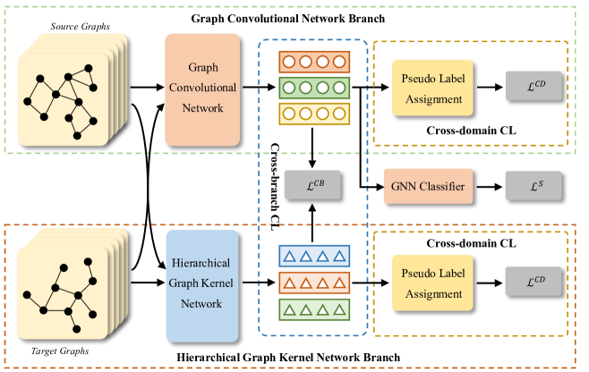
Figure 1: An overview of the proposed CoCo. Our CoCo feeds source graphs and target graphs into two branches (i.e., GCN branch and HGKN branch). Cross-branch contrastive learning compares graph representations from two branches to achieve while cross-branch contrastive learning compares graph representations from two domains with the guidance of pseudo-labels.

2.2 Unsupervised Domain Adaptation

The purpose of unsupervised domain adaptation (UDA) is to transfer a model from a label-rich source domain to a label-scarce target domain (He et al., 2022; Huang et al., 2022; Nguyen et al., 2022; Wang et al., 2022). This problem is substantially investigated in the field of computer vision with applications in image classification (Mirza et al., 2022), image retrieval (Zheng et al., 2021) and semantic segmentation (Kundu et al., 2022). In general, domain alignment is the key to successful domain adaptation. The early attempts usually explicitly reduce domain discrepancy using statistical metrics including maximum mean discrepancy (Long et al., 2015) and Wasserstein distance (Shen et al., 2018). Recently, adversarial learning-based approaches are the predominant paradigm for UDA (Long et al., 2018). These methods usually employ a gradient reversal layer (Ganin et al., 2016) to render deep features resistant to domain shifts. In addition, discrimination learning under label scarcity is an important challenge for UDA (Xiao & Zhang, 2021; Liang et al., 2020) and pseudo-labeling techniques are popular strategies (Lee et al., 2013; Assran et al., 2021) to tackle this problem in the target domain. Despite the significant advance of UDA in computer vision, it is still underexplored in the graph domain. In this work, we study the emerging and practical problem of unsupervised domain adaptive graph classification, which employs labeled source graphs to improve the classification performance on unlabeled target graphs. Different from existing domain adaptation methods (Yin et al., 2022a; Mirza et al., 2022; Wei et al., 2021a), our CoCo explores semantics information from different views and conduct coupled contrastive learning for effective domain adaptation.

3 Methodology

The overview of the proposed CoCo framework for unsupervised domain adaptive graph classification is illustrated in Figure 1. The core of our CoCo is to provide two complementary views to explore graph topology using coupled branches. From an implicit view, we utilize a graph convolutional network branch to infer topological information (see Section 3.2), while a hierarchical graph kernel network branch is adopted to compare graph samples with learnable filters (see Section 3.3), which explicitly summarizes topological information. Moreover, we incorporate the two branches into a holistic multi-view contrastive learning framework (see Section 3.4). On the one hand, we perform cross-branch contrastive learning to encourage the agreement of two branches for representations containing comprehensive structural information. On the other hand, cross-domain contrastive learning aims to minimize the distances between cross-domain sample pairs with the same semantics compared to those with different semantics.

3.1 Problem Formulation

Given a graph $G=(\mathcal{V},\mathcal{E})$, in which $\mathcal{V}$ is the set of nodes and $\mathcal{E}\subseteq\mathcal{V}\times\mathcal{V}$ denotes the set of edges. There is also a node feature matrix $\bm{X}\in\mathbb{R}^{|\mathcal{V}|\times d}$, where each row $\bm{x}_{v}\in\mathbb{R}^{d}$ denotes the feature of node $v\in\mathcal{V}$, $|\mathcal{V}|$ is the number of nodes, and $d$ denotes the dimension of node features. In our problem, we have access to a labeled source domain $\mathcal{D}^{s}=\{(G_{i}^{s},y_{i}^{s})\}_{i=1}^{n_{s}}$ with $n_{s}$ samples and an unlabeled target domain $\mathcal{D}^{t}=\{G_{j}^{t}\}_{j=1}^{n_{t}}$ with $n_{t}$ samples. $\mathcal{D}^{s}$ and $\mathcal{D}^{t}$ share the label space, i.e., $\mathcal{Y}=\{1,2,\cdots,C\}$ with different distributions in the data space. We expect to train the graph classification model using both $\mathcal{D}^{s}$ and $\mathcal{D}^{t}$, and attain high accuracy on the test dataset on the target domain.

3.2 Graph Convolutional Network Branch

In this branch, we utilize a graph convolutional network to implicitly extract topological information. Graph convolutional networks (GCNs) typically follow the message-passing scheme to embed the structural and attribute information into node representations, which have shown their superior capability in graph classification (Gilmer et al., 2017; Kipf & Welling, 2017; Xu et al., 2019). In detail, for each node, we start by aggregating the embedding vectors of all its neighbors at the previous layer. Then the node representation is updated iteratively by fusing the representation from the last layer with the aggregated neighbor embedding. In formulation, the representation of node $v\in G$ at the $l$-th layer $\bm{h}_{v}^{(l)}$ is calculated as follows:

$$\bm{h}_{v}^{(l)}=\operatorname{COM}^{(l)}_{\theta}\left(\bm{h}_{v}^{(l-1)},\operatorname{AGG}^{(l)}_{\theta}\left(\left\{\bm{h}_{u}^{(l-1)}\right\}_{u\in\mathcal{N}(v)}\right)\right),$$

where $N(v)$ denotes the neighbors of $v$. $\operatorname{AGG}^{(l)}_{\theta}$ and $\operatorname{COM}^{(k)}_{\theta}$ denote the aggregation and combination operations parameterized by $\theta$ at the $l$-th layer, respectively. Ultimately, we adopt an extra $\operatorname{READOUT}$ function to summarize the node representations at the last layer into a graph-level representation. In formulation,

$$g_{\theta}\left(G\right)=\operatorname{READOUT}\left(\left\{\bm{h}_{v}^{(L)}\right\}_{v\in V}\right),$$ (1)

where $g_{\theta}\left(G\right)$ denotes the graph-level representation and the network parameters are denoted by $\theta$.

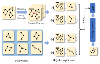
Figure 2: An illustration of the hierarchical graph kernel network branch. HGKN compares each $r$-hop subgraph with filter graphs to generate node features, followed by an attention-based pooling operation to coarsen the graph.

3.3 Hierarchical Graph Kernel Network Branch

However, GCNs are insufficient in collecting sophisticated high-order structural information such as rings (Long et al., 2021; Cosmo et al., 2021). Consequently, it is anticipated to explore graph topology in an explicit manner as a compliment. To accomplish this, we introduce a hierarchical graph kernel network (HGKN) based on a graph kernel (e.g., WL kernel, random walk kernel). Generally, at each hierarchical layer, it compares each $r$-hop subgraph with learnable filter graphs via the graph kernel to update node representations, followed by an attention-based pooling operation to coarsen the graph. After multiple hierarchical layers, a graph-level representation can be obtained in an end-to-end manner.

To be specific, for each graph, we first extract the local information of each node using its $r$-hop subgraph, which comprises all nodes reached by the central node within $r$ edges, along with all the edges between these selected nodes. To explore topological information from these subgraphs, we generate $M$ undirected learnable graphs with varying sizes serving as filters, i.e., $\{\tilde{G}_{1}^{(k)},\cdots,\tilde{G}_{M}^{(k)}\}$ at the $k$-th layer. Each of the filter graphs $\tilde{G}_{m}^{(k)}$ is with a trainable adjacency matrix and each node is with an attribute. We expect these learnable filters to extract high-order structural information for better graph classification. However, most of the graph kernels usually accompany with discrete node attributes (Cosmo et al., 2021; Schulz & Welke, 2019). To tackle this, we introduce a quantization operation $Q(\cdot)$, which discretizes node attributes using clustering during network forwarding. Through $Q(\cdot)$, the continuous attributes are replaced by the discrete cluster assignments. Then, we compare the discrete input graph and the filter graphs using the graph kernel.

$$e_{v}^{(k)}(m)=\Phi(Q(S_{v}^{(k-1)}),\tilde{G}_{m}^{(k)}),$$ (2)

where $S_{v}^{(k-1)}$ denotes the subgraph with center $v$ at the previous layer and $\Phi(\cdot,\cdot)$ denotes the given graph kernel. Then, we can update the node representation $\bm{e}_{v}^{(k)}\in\mathbb{R}^{M}$ by concatenating all the output of filters as follows:

$$\bm{e}_{v}^{(k)}=[e_{v}^{(k)}(1),\cdots,e_{M}^{(v)}(M)].$$ (3)

Finally, we utilize a multi-layer perceptron (MLP) $\psi^{k}(\cdot)$ to project the concatenated kernel values into node representations at the $k$-th layer, i.e., $\bm{x}_{v}^{(k)}=\psi^{k}(\bm{e}_{v}^{(k)})$.

To address the issue that the quantization operation cannot be compatible with stochastic gradient descent, we merely calculate the gradient with respect to the filters in each layer of the graph kernel network during backpropagation. This strategy has been extensively used when optimizing the deep hashing networks, exhibiting satisfactory performance empirically (Tan et al., 2020; Qiu et al., 2021). In addition, we utilize a discrete algorithm to update filter graphs using the edit operation which includes adding (removing) edges and modifying node attributes. To be specific, for each $\tilde{G}_{m}^{k}$, we conduct a random edit operation candidate $\tilde{G^{\prime}}_{m}^{k}$ and determine whether to accept it based on the gradient of the loss with respect to the filters. In formulation,

$$\frac{\partial\mathcal{L}}{\partial\tilde{G}_{m}^{k}}=\sum_{v\in G}\frac{\partial\mathcal{L}}{\partial e_{v}^{(k)}(m)}\frac{\partial e_{v}^{(k)}(m)}{\partial\tilde{G}_{m}^{k}}.$$ (4)

However, we cannot acquire ${\partial e_{v}^{(k)}(m)}/{\partial\tilde{G}_{m}^{k}}$. Instead, we utilize the difference between kernel values of candidate $\tilde{G^{\prime}}_{m}^{k}$ and original filter $\tilde{G}_{m}^{k}$, i.e., $\Phi(Q(S_{v}^{(k-1)}),\tilde{G^{\prime}}_{m}^{(k)})-\Phi(Q(S_{v}^{(k-1)}),\tilde{G}_{m}^{(k)})$ to replace it. After estimating ${\partial\mathcal{L}}/{\partial\tilde{G}_{m}^{k}}$, we will accept the candidate if the gradient is above zero and vice versa.

As in convolutional neural network (CNN) architectures (Passalis & Tefas, 2018), after computing the graph kernel, we additionally introduce a pooling operation (Lee et al., 2019) using the attention mechanism to provide a hierarchical view while reducing the computational cost. To be specific, we utilize an MLP to produce score vector $Z\in\mathbb{R}^{|V^{(k)}|\times 1}$ for each graph, where $V^{(k)}$ represents the set of nodes at the $k$-th layer. On the basis of scores, the top $\lceil\rho|V^{(k)}|\rceil$ nodes are kept with an index set $idx$ where $\rho\in(0,1)$ is the pooling ratio. In the end, we calculate the pooled graph $G_{pool}^{(k)}$ with the attribute matrix $\bm{X}_{pool}^{(k)}$ and adjacent matrix $A_{pool}^{(k)}$. The learnt node representations are first concatenated into a matrix $\bm{X}^{(k)}$. Let $\odot$ denote the broadcasted Hadamard product, and we have:

$$X^{(k)}_{pool}=X^{(k)}_{idx,:}\odot Z_{idx},A^{(k)}_{pool}=A^{(k)}_{idx,idx},$$ (5)

where $X^{(k)}_{idx,:}$, $A^{(k)}_{idx,idx}$ denote the node-indexed feature matrix and the row, column-indexed adjacency matrix.

After multiple hierarchical graph kernel layers followed by graph pooling operations, we feed all the node feature $\bm{e}_{v}^{(K)}$ into a fully-connected layer followed by a sum-pooling to produce a graph-level representation denoted as $f_{\phi}(\mathcal{G})$.

3.4 Multi-view Contrastive Learning Framework

To fully exploit graph topology information derived from two branches, we formalize a multi-view contrastive learning framework, which contains both cross-branch and cross-domain contrastive learning for effective domain adaptation.

Cross-branch Contrastive Learning. Considering that the model learns graph semantics from complementary views, we contrast the graph representations from two branches to exchange their knowledge mutually, which enhances discrimination learning on target data under label scarcity.

Specifically, for each a graph $G_{i}$ in a source batch $\mathcal{B}^{s}$ and a target batch $\mathcal{B}^{t}$, we produce the embeddings from coupled branches, i.e., $\bm{z}_{i}=g_{\theta}(G_{i})$ and $\tilde{\bm{z}}_{i}=f_{\phi}(G_{i})$. Then, we introduce the InfoNCE loss to enhance the consistency cross coupled branches. In formulation,

$$\mathcal{L}^{CB}\!=\!\frac{1}{|\mathcal{B}^{s}|+|\mathcal{B}^{t}|}\sum_{G_{i}\in\mathcal{B}^{s}\cup\mathcal{B}^{t}}\!\!-\!\log\frac{exp(\bm{z}_{i}\ast\tilde{\bm{z}}_{i}/\tau)}{\sum_{G_{i^{\prime}}\in\mathcal{B}^{t}}exp({\bm{z}_{i}\ast\tilde{\bm{z}}_{i^{\prime}}/\tau})},$$ (6)

where $\tau$ represents a temperature parameter set to $0.5$ as in previous works (He et al., 2020). Through providing challenging views by mining topological information in complementary manners, our proposed CoCo is a special kind of graph contrastive learning (You et al., 2020, 2021; Yin et al., 2022b), hence producing discriminative graph-level representation with sufficient topological information.

Cross-domain Contrastive Learning. However, with a serious domain shift in the graph space, the graph representations could remain biased and unreliable for downstream classification. Intuitively, the representations of source (target) samples should be close to target (source) samples with the same semantics. To achieve this, we need to generate pseudo-labels of target data as a preliminary. In light of the fact that learning a classifier is suboptimal and biased owing to the paucity of labels, we generate pseudo-labels in a non-parametrical manner by comparing the similarities between target graphs and source graphs. On this basis, we conduct cross-domain contrastive learning which minimizes the distances between cross-domain example pairs with the same semantics compared to those with different semantics.

Taking the GCN branch as an example, we utilize a non-parametrical classifier to generate the pseudo-label for each $G_{j}^{t}$. In formulation, we have:

$$\hat{p}_{j}^{t}=\sum_{(G_{i}^{s},y_{i}^{s})\in\mathcal{B}^{s}}\left(\frac{\zeta\left(\bm{z}_{j},g_{\theta}(G_{i}^{s})\right)}{\sum_{(G_{i}^{s},y_{i}^{s})\in\mathcal{B}^{s}}\zeta\left(\bm{z}_{j},g_{\theta}(G_{i}^{s})\right)}\right)\bm{y}_{i}^{s},$$ (7)

where $\bm{y}_{i}^{s}$ denotes the one-hot label embedding and $\zeta\left(\bm{z}_{j},g_{\theta}(G_{i}^{s})\right)=exp(\bm{z}_{j}\ast g_{\theta}(G_{i}^{s})/\tau)$ denotes the similarities between two vectors. In Eq. 7, we involve a batch of labeled source data in the classifier for efficiency. The pseudo-labels can be easily derived from $\hat{p}_{j}^{t}$, i.e., $\hat{y}^{t}_{j}=\arg max(\hat{p}_{j}^{t})$.

Then, we pull close the representations with the same semantics across domains to minimize domain discrepancy. To achieve this, we treat the source samples with identical labels as positives for each target sample. In formulation, we set $\Pi(j)=\{i|y_{i}^{s}=\hat{y}^{t}_{j},G_{i}^{s}\in\mathcal{B}^{s}\}$ to represent the index of all positives in the mini-batch and the cross-domain contrastive learning objective is written as:

$$\mathcal{L}^{CD}=\sum_{G_{j}^{t}\in\mathcal{B}^{t}}\frac{-1}{|\Pi(j)|}\sum_{i\in\Pi(j)}\log\frac{\exp\left(\bm{z}_{j}^{t}\ast\bm{z}_{i}^{s}/\tau\right)}{\sum_{G_{i^{\prime}}^{s}\in\mathcal{B}^{s}}\exp\left(\bm{z}_{j}^{t}\ast\bm{z}_{i^{\prime}}^{s}/\tau\right)}.$$ (8)

Our cross-domain contrastive learning objective has two benefits. On the one hand, given that the numerator of each term penalizes the distances between source samples and target samples with the same semantics, our loss contributes to generating domain-invariant graph representations. On the other hand, due to the promising results achieved by contrastive learning (You et al., 2020; Li et al., 2020; Khosla et al., 2020; Huang et al., 2021), comparing positive pairs with negative pairs can aid in developing discriminative graph representations for effective graph classification under label scarcity. We also construct the contrastive learning objective in the other branch and sum them to get the final loss. In addition, we demonstrate that our cross-domain contrastive learning can be interpreted as maximizing the log-likelihood on target data using an Expectation Maximization (EM) algorithm. Compared with previous contrastive learning work (He et al., 2020; Chen et al., 2020b), our model utilizes a coupled framework which includes cross-module contrastive learning and cross-domain contrastive learning, which follow the paradigm of the EM algorithm while contrastive learning on images usually utilizes the InfoNCE loss to maximize the consistency.

Proposition 3.1.

The cross-domain contrastive framework follows the EM algorithm.

The proof of Proposition 3.1 can be found in Appendix A.

Algorithm 1 Learning Algorithm of CoCo

Input: Source data $\mathcal{D}^{s}$; Target data $\mathcal{D}^{t}$.

Output: GCN parameters $\theta$, HGKN parameters ${\phi}$, Classifier parameters $\eta$.

1:  Initialize model parameters.

2:  while not convergence do

3:     Sample mini-batches $\mathcal{B}^{s}$ and $\mathcal{B}^{t}$ from source and target data, respectively;

4:     Forward propagation $\mathcal{B}^{s}$ and $\mathcal{B}^{t}$ through two branches;

5:     Calculate the loss function in Eq. 10;

6:     Update model parameters through back propagation;

7:  end while

3.5 Summarization

To produce label distributions of test data, we utilize enhanced graph representations from the first branch to predict the label via a fully-connected layer. The reason for selecting the first branch is that the single GCN is more efficient than a single HGKN during evaluation. In CoCo, we adopt the standard cross entropy $H(\cdot,\cdot)$ to formulate the supervised objective as follows:

$$\mathcal{L}^{S}=\frac{1}{|\mathcal{B}^{s}|}\sum_{G_{i}^{s}\in\mathcal{B}^{s}}H(\hat{y}_{i}^{s},y_{i}^{s}),$$ (9)

where $\hat{y}_{i}^{s}$ denotes the output of the classifier. In a nutshell, we combine two contrastive learning objectives with a supervised objective. The overall loss objective is:

$$\mathcal{L}=\mathcal{L}^{CB}+\mathcal{L}^{CD}+\mathcal{L}^{S}.$$ (10)

The algorithmic overview of CoCo is depicted in Algorithm 1. The computing complexity of the proposed CoCo primarily relies on two networks. For a given graph $G$, $||A||_{0}$ denotes the number of nonzeros in the adjacency matrix. $d$ is the feature dimension. $L$ and $K$ denote the layer number of GCN and HGKN, respectively. $|V|$ is the number of nodes. $M$ denotes the number of filter graphs. The graph convolutional network takes $\mathcal{O}(L||A||_{0}d+L|V|d^{2})$ computational time while the graph kernel module takes $\mathcal{O}(K|V|M)$ for each graph. As a result, the complexity of our CoCo is proportional to both $|V|$ and $||A||_{0}$.

4 Experiments

Table 1: The classification results (in %) on Mutagenicity (source$\rightarrow$target).

Methods	M0$\rightarrow$M1	M1$\rightarrow$M0	M0$\rightarrow$M2	M2$\rightarrow$M0	M0$\rightarrow$M3	M3$\rightarrow$M0	M1$\rightarrow$M2	M2$\rightarrow$M1	M1$\rightarrow$M3	M3$\rightarrow$M1	M2$\rightarrow$M3	M3$\rightarrow$M2	Avg.
GCN	71.1	70.4	62.7	69.0	57.7	59.6	68.8	74.2	53.6	63.3	65.8	74.5	65.9
WL subtree	74.9	74.8	67.3	69.9	57.8	57.9	73.7	80.2	60.0	57.9	70.2	73.1	68.1
CDAN	73.8	74.1	68.9	71.4	57.9	59.6	70.0	74.1	60.4	67.1	59.2	63.6	66.7
ToAlign	74.0	72.7	69.1	65.2	54.7	73.1	71.7	77.2	58.7	73.1	61.5	62.2	67.8
MetaAlign	66.7	51.4	57.0	51.4	46.4	51.4	57.0	66.7	46.4	66.7	46.4	57.0	55.4
GIN	72.3	68.5	64.1	72.1	56.6	61.1	67.4	74.4	55.9	67.3	62.8	73.0	66.3
CIN	66.8	69.4	66.8	60.5	53.5	54.2	57.8	69.8	55.3	74.0	58.9	59.5	62.2
GMT	73.6	75.8	65.6	73.0	56.7	54.4	72.8	77.8	62.0	50.6	64.0	63.3	65.8
DUA	70.2	56.5	64.0	63.7	53.6	68.5	57.7	76.0	65.1	59.8	57.9	67.7	63.4
CoCo	77.7	76.6	73.3	74.5	66.6	74.3	77.3	80.8	67.4	74.1	68.9	77.5	74.1

Table 2: The classification results (in %) on Tox21 (source$\rightarrow$target).

Methods	T0$\rightarrow$T1	T1$\rightarrow$T0	T0$\rightarrow$T2	T2$\rightarrow$T0	T0$\rightarrow$T3	T3$\rightarrow$T0	T1$\rightarrow$T2	T2$\rightarrow$T1	T1$\rightarrow$T3	T3$\rightarrow$T1	T2$\rightarrow$T3	T3$\rightarrow$T2	Avg.
GCN	64.2	50.3	67.9	50.4	52.2	53.8	68.7	61.9	59.2	51.4	54.9	76.3	59.3
WL subtree	65.3	51.1	69.6	52.8	53.1	54.4	71.8	65.4	60.3	61.9	57.4	76.3	61.6
CDAN	69.9	55.2	78.3	56.0	59.5	56.6	78.3	68.5	61.7	68.1	61.0	78.3	66.0
ToAlign	68.2	58.5	78.4	58.8	58.5	53.8	78.8	67.1	64.4	68.8	57.9	78.4	66.0
MetaAlign	65.7	57.5	78.0	58.5	63.9	52.2	78.8	67.1	62.3	67.5	56.8	78.4	65.6
GIN	67.8	51.0	77.5	54.3	56.8	54.5	78.3	63.7	56.8	53.3	56.8	77.1	62.3
CIN	67.8	50.3	78.3	54.5	56.8	54.5	78.3	67.8	59.0	67.8	56.8	78.3	64.2
GMT	67.8	50.0	78.4	50.1	56.8	50.7	78.3	67.8	56.8	67.8	56.4	78.1	63.3
DUA	60.6	51.3	70.7	52.5	53.6	49.3	71.1	67.2	53.6	59.0	58.6	74.3	60.2
CoCo	69.9	59.8	78.8	59.0	62.3	59.0	78.4	66.8	65.0	68.8	61.2	78.4	67.3

Table 3: The classification results (in %) on PROTEINS, COX2, and BZR (source$\rightarrow$target).

Methods	P$\rightarrow$D	D$\rightarrow$P	C$\rightarrow$CM	CM$\rightarrow$C	B$\rightarrow$BM	BM$\rightarrow$B	Avg.
GCN	58.7	59.6	51.1	78.2	51.3	71.2	61.7
WL subtree	72.9	41.1	48.8	78.2	51.3	78.8	61.9
CDAN	59.7	64.5	59.4	78.2	57.2	78.8	66.3
ToAlign	62.6	64.7	51.2	78.2	58.4	78.7	65.7
MetaAlign	60.3	64.7	51.0	77.5	53.6	78.5	64.3
GIN	61.3	56.8	51.2	78.2	48.7	78.8	62.5
CIN	62.1	59.7	57.4	61.5	54.2	72.6	61.3
GMT	62.7	59.6	51.2	72.2	52.8	71.3	61.6
DUA	61.3	56.9	51.3	69.5	56.4	70.2	60.9
CoCo	74.6	67.0	61.1	79.0	62.7	78.8	70.5

Table 4: The results of ablation studies on Mutagenicity (source$\rightarrow$target).

Methods	M0$\rightarrow$M1	M1$\rightarrow$M0	M0$\rightarrow$M2	M2$\rightarrow$M0	M0$\rightarrow$M3	M3$\rightarrow$M0	M1$\rightarrow$M2	M2$\rightarrow$M1	M1$\rightarrow$M3	M3$\rightarrow$M1	M2$\rightarrow$M3	M3$\rightarrow$M2	Avg.
CoCo/CB	78.0	72.2	63.8	71.4	62.1	69.1	76.0	77.3	64.1	74.8	65.4	76.3	70.9
CoCo/CD	74.0	72.7	65.8	65.9	58.6	69.4	71.5	78.3	66.6	74.9	66.2	75.6	70.0
CoCo-GIN	74.9	73.6	63.6	70.7	58.3	70.0	76.6	78.5	66.5	75.1	66.7	77.5	71.0
CoCo-HGKN	74.9	73.0	64.5	70.5	63.0	70.6	76.3	78.0	66.1	74.7	66.4	77.3	71.3
CoCo	77.7	76.6	73.3	74.5	66.6	74.3	77.3	80.8	67.4	74.1	68.9	77.5	74.1
CoCo-NP	77.2	76.0	74.1	74.2	65.5	74.6	77.7	81.0	67.1	74.7	69.2	76.1	74.0

4.1 Experimental Settings

Datasets. We perform experiments on various real-world benchmark datasets (i.e., Mutagenicity, Tox21, PROTEINS, DD, BZR and COX2) from TUDataset (Morris et al., 2020) in the setting of unsupervised domain adaptation. For convenience, P, D, C, CM, B, and BM are short for PROTEINS, DD, COX2, COX2_MD, BZR, and BZR_MD, respectively. Their details are introduced as follows:

• Mutagenicity (Kazius et al., 2005): Mutagenicity is a popular dataset that consists of 4337 molecular structures and their corresponding Ames test data. To distinguish the distribution of datasets, we divide it into four sub-datasets (i.e., M0, M1, M2 and M3) based on the edge density.

• Tox21: The purpose of the Tox21 dataset is to assess the predictive ability of models in detecting compound interferences. We separate the dataset into four sub-datasets according to their interactions with ‘aromatase’ and ‘HSE’.

• PROTEINS: PROTEINS (Dobson & Doig, 2003) and DD (Shervashidze et al., 2011) are investigated here and each label indicates if a protein is a non-enzyme or not. The presentation of each protein is in the form of a graph, where the amino acids serve as nodes and edges exist when the distance between two nodes is less than 6 Angstroms.

• COX2: We investigate datasets COX2 and COX2_MD (Sutherland et al., 2003) which consists of 467 and 303 cyclooxygenase-2 inhibitors. Every sample characterizes a chemical compound, with edges determined by distance and vertex features representing atom types.

• BZR: We explore the BZR and BZR_MD (Sutherland et al., 2003) datasets, which contains ligands for the benzodiazepine receptor.

Baselines. To increase persuasiveness, we compare the proposed CoCo with a large number of state-of-the-art methods, including one graph kernel approach (WL subtree (Shervashidze et al., 2011)), four graph neural network methods (GCN (Kipf & Welling, 2017), GIN (Xu et al., 2019), CIN (Bodnar et al., 2021) and GMT (Baek et al., 2021)), and four recent domain adaptation methods (CDAN (Long et al., 2018), ToAlign (Wei et al., 2021b), MetaAlign (Wei et al., 2021a) and DUA (Mirza et al., 2022)). Their detailed introduction is elaborated in Appendix B.

Implementation Details. We employ a two-layer GIN (Xu et al., 2019) in the GCN branch and a two-layer network along with the WL kernel (Shervashidze et al., 2011) in the HGKN branch. We use the Adam as the default optimizer and set the learning rate to $10^{-4}$. The embedding dimension of hidden layers and batch size are both set to 64. The pooling ratio $\rho$ and the number of filter graphs $M$ are set to $0.4$ and $15$, respectively. For the sake of fairness, we employ the same GCN as the graph encoder. In the graph classification baselines in all domain adaption baselines. We utilize all the labeled source samples to train the model and evaluate unlabeled samples when it comes to graph classification methods as in (Wu et al., 2020a). We initialize the parameters of all the compared methods as in their corresponding papers and fine-tune them to achieve the best performance.

4.2 Performance Comparison

Table 1, 2 and 3 show the performance of graph classification in various settings of unsupervised domain adaptation. From the results, we observe that: 1) The domain adaptation methods generally perform better than graph kernel and GNN methods in Table 2 and 3, indicating that current graph classification models are short of the capacity of transfer learning. Thus, it is essential to design an effective domain adaptive framework for graph classification. 2) Although the domain adaptation methods obtain competitive results on simple transfer tasks in Table 3, it is difficult for them to make great progress on hard transfer tasks in comparison with GIN (Table 1). We attribute the reason to the immense difficulty of acquiring graph representations. Therefore, it is unwise to directly apply current domain adaptation approaches to GCNs. 3) Our CoCo outperforms all the baselines in most cases. In particular, the average improvement of CoCo ranges is 8.81% on Mutagenicity. We attribute the performance gain to two key points: (i) Contrastive learning across coupled branches (i.e., GCN and HGKN) improves the representation ability of graphs under label scarcity. (ii) Cross-domain contrastive learning contributes to effective domain alignment from an EM perspective.

4.3 Effect of Different GNNs and Graph Kernels

To investigate the flexibility of CoCo, we replace the GIN in our implementation with different GNN methods (i.e., GCN (Kipf & Welling, 2017), GAT (Veličković et al., 2018) and Graphsage (Hamilton et al., 2017)) and the WL kernel with different graph kernels (i.e., Graph Sampling (Leskovec & Faloutsos, 2006), Random Walk (Kalofolias et al., 2021) and Propagation (Neumann et al., 2016)). Figure 3 shows the performance of different GNNs and graph kernels on two representative datasets, and we have similar observations on other datasets. From the results, we have the following observation, by comparing with other GCN architectures and graph kernels, GIN and WL kernels achieve the best performance in most of the cases and the reason can be attributed to the powerful representation capability of GIN and WL kernel. This also justifies the motivation why we select WL kernel to improve the performance in our task of domain adaptation.

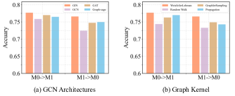
Figure 3: The performance with different GCN architectures and graph kernels on Mutagenicity.

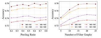
Figure 4: Sensitivity analysis on Mutagenicity. We select four transfer learning tasks here.

4.4 Ablation Study

To evaluate the impact of each component in our CoCo, we introduce several model variants as follows: 1) CoCo/CB: It removes the cross-branch contrastive learning module; 2) CoCo/CD: It removes the cross-domain contrastive learning module; 3) CoCo-GIN: It uses two distinct GINs to generate coupled graph representations; 4) CoCo-HGKN: It uses two distinct HGKN to generate coupled graph representations. 5) CoCo-NP: It utilizes the non-parametric classifier instead of the MLP classifier for target domain prediction.

We compare the performance on Mutagenicity and the results are shown in Table 4. From Table 4, we have the following observations: 1) CoCo/CB exhibits inferior performance compared with the CoCo in most settings, validating that comparing complementary information extracted by GCN and HGKN is capable of improving graph representation learning. 2) CoCo/CD obtain the worst performance among four model variants, we attribute the reason to that the cross-domain contrastive learning module aligns the source and target graph representations effectively, which tackles serious domain discrepancy in the graph space. This challenge is the most crucial in our task. 3) CoCo-GIN and CoCo-HGKN achieves approximate results but performs worse than CoCo, which demonstrates that merely ensemble learning in the implicit (explicit) manner cannot largely enhance graph representation learning under label scarcity. 4) The average performance of CoCo and CoCo-NP is quite similar. The reason is that after sufficient training, the performance of the non-parametric classifier and the MLP classifier is similar. However, the non-parametric classifier demands a substantial amount of labeled source domain data, resulting in significantly lower efficiency compared to the MLP classifier. Consequently, we recommend employing the MLP classifier for target domain prediction.

4.5 Sensitivity Analysis

In this part, we investigate the sensitivity of the proposed CoCo to the hyper-parameters (i.e., pooling ratio $\rho$ and number of filter graphs $M$) that affect the performance of CoCo. $\rho$ determines the number of kept nodes of pooled graphs, and $M$ denotes the number of filters. Figure 4 plots the results on Mutagenicity. We first vary $\rho$ in the set from 0.2 to 0.8 with other parameters fixed. The performance generally shows an increasing trend at the beginning and stabilizes as the ratio of $\rho$ increases. We attribute the reason to the small $\rho$ keeping fewer nodes which may miss some important information. On the contrary, the larger $\rho$ retains more node information, but the complexity of the model is greatly increased. Considering the trade-off between model performance and complexity, we set $\rho$ to 0.4 as default. In addition, We vary $M$ in {5, 10, 15, 20, 25} while fixing other parameters. It can be found that with the increasing of $M$, the CoCo achieves better performance when the value is small. The potential reason is that increasing the number of filter graphs would help to extract high-order structure information. Nevertheless, when $M$ is too large (i.e., $M>15$), the improvement in performance is not obvious. Thus, to balance the performance with the computational complexity, we set $M$ to 15.

5 Conclusion

This paper addresses the practical problem of unsupervised graph classification and introduces an effective method named CoCo is proposed. At a high level, CoCo is featured by two branches, i.e., a graph convolutional network branch and a hierarchical graph kernel network branch, which explores graph topological information in implicit and explicit manners, respectively. Then, we integrate the two branches into a multi-view contrastive learning framework where cross-branch contrastive learning aims to generate discriminative graph representation with full semantics whereas cross-domain contrastive learning strives to minimize domain discrepancy. Extensive experiments on diverse datasets validate the efficacy of proposed CoCo compared with various competing methods. In future works, we will extend our proposed CoCo to address more complicated tasks, including domain generalization, multi-source domain adaptation and source-free domain adaptation.

Appendix A An Expectation-Maximization Perspective

Maximum Likelihood (ML) has been widely utilized in various unsupervised machine learning problems (Sharma et al., 2016; Li et al., 2020; Gresele et al., 2020). In our settings, it aims to find the optimal weights of the graph encoder $\theta^{*}$ to maximize the log-likelihood of target graphs within a mini-batch. In formulation, the log-likelihood function is written as:

$$\ell_{likelihood}(\theta)=\sum_{G_{j}^{t}\in\mathcal{B}^{t}}\log p(G_{j}^{t};\theta).$$ (11)

To make use of abundant labeled source graphs, the unlabeled sample $G_{j}^{t}\in\mathcal{B}^{t}$ are compared with source graphs in a mini-batch, denoted as $\{G_{i}^{s}\}_{i=1}^{B^{s}}$ for clearness, and we have:

$$\theta^{*}=\mathop{\arg\max}\limits_{\theta}\sum_{G_{j}^{t}\in\mathcal{B}^{t}}\log\sum_{i=1}^{B^{s}}p(G_{j}^{t},G_{i}^{s};\theta).$$ (12)

However, directly optimizing the function would be difficult. To tackle this, we introduce a surrogate function $Q(G_{i}^{s})$ $(\sum_{i=1}^{B^{s}}Q(G_{i}^{s})=1)$ to estimate the lower-bound of Eq. 12. By applying Jensen’s inequality, we have:

$$\sum_{G_{j}^{t}\in\mathcal{B}^{t}}\log\sum_{i=1}^{B^{s}}p(G_{j}^{t},G_{i}^{s};\theta) =\sum_{G_{j}^{t}\in\mathcal{B}^{t}}\log\sum_{i=1}^{B^{s}}Q(G_{i}^{s})\frac{p(G_{j}^{t},G_{i}^{s};\theta)}{Q(G_{i}^{s})}$$ (13)

$$\geq\sum_{G_{j}^{t}\in\mathcal{B}^{t}}\sum_{i=1}^{B^{s}}Q(G_{i}^{s})\log\frac{p(G_{j}^{t},G_{i}^{s};\theta)}{Q(G_{i}^{s})}.$$

The equality holds when $Q(G_{i}^{s})/p(G_{i}^{s},G_{j}^{t};\theta)$ is a constant, which results in the following formulation:

$$\frac{Q(G_{i}^{s})}{p(G_{i}^{s},G_{j}^{t};\theta)}=\frac{\sum_{i=1}^{B^{s}}Q(G_{i}^{s})}{\sum_{i=1}^{B^{s}}p(G_{i}^{s},G_{j}^{t};\theta)}=\frac{1}{p(G_{j}^{t};\theta)}.$$ (14)

Hence, we have $Q(G_{i}^{s})=p(G_{i}^{s};G_{j}^{t},\theta)$.

It is worth noting that $-\sum_{G_{j}^{t}\in\mathcal{B}^{t}}\sum_{i=1}^{B^{s}}Q(G_{i}^{s})\log Q(G_{i}^{s})$ does not influence the optimization of $\theta$. Therefore, we rewrite the objective function as follows:

$$\ell=\sum_{G_{j}^{t}\in\mathcal{B}^{t}}\sum_{i=1}^{B^{s}}p(G_{i}^{s};G_{j}^{t},\theta)\log p(G_{j}^{t},G_{i}^{s};\theta),$$ (15)

Then, we utilize an EM algorithm to maximize Eq. 15.

E step. This step aims to infer the posterior probability $p(G_{i}^{s};G_{j}^{t},\theta)$. To begin with, we calculate the pseudo-label of the target data $G_{j}^{t}$ using $g_{{\theta}}$ where ${\theta}$ denotes the current model parameters. Treating all source samples with the same label equally, we have $p(G_{i}^{s};G_{j}^{t},\theta)=\frac{1}{|\Pi(j)|}\mathbbm{1}(G_{j}^{t},G_{i}^{s})$ where $\mathbbm{1}(G_{j}^{t},G_{i}^{s})=1$ if they has the same label and $|\Pi(j)|=\sum_{i=1}^{B^{s}}\mathbbm{1}(G_{j}^{t},G_{i}^{s})$ denotes the number of source samples with the same label.

M step. This step aims to maximize the lower-bound of Eq. 15 based on E-step. In particular, we have:

$$\ell =\sum_{G_{j}^{t}\in\mathcal{B}^{t}}\sum_{i=1}^{B^{s}}p(G_{i}^{s};G_{j}^{t},\theta)\log p(G_{j}^{t},G_{i}^{s};\theta)$$ (16)

$$=\sum_{G_{j}^{t}\in\mathcal{B}^{t}}\sum_{i=1}^{B^{s}}\frac{1}{|\Pi(j)|}\mathbbm{1}(G_{j}^{t},G_{i}^{s})\log p(G_{j}^{t},G_{i}^{s};\theta).$$

When presuming the prior obeys a uniform distribution and employing an isotropic Gaussian to characterize the distribution of each sample in the embedding space, we have:

$$p(G_{j}^{t},G_{i}^{s};\theta )=p(G_{j}^{t};G_{i}^{s},\theta)p(G_{i}^{s};\theta)=\frac{1}{{B^{s}}}\cdot p(G_{j}^{t};G_{i}^{s},\theta),$$ (17)

$$p(G_{j}^{t};G_{i}^{s},\theta) =\exp(\frac{-(\bm{z}_{j}^{t}-\bm{z}_{i}^{s})^{2}}{2\sigma_{i}^{2}})/\sum_{i^{\prime}=1}^{B^{s}}\exp(\frac{-(\bm{z}_{j}^{t}-\bm{z}^{s}_{i^{\prime}})^{2}}{2\sigma_{i^{\prime}}^{2}}),$$

where $\bm{z}_{j}^{t}=g_{\phi}(G_{j}^{t})$ and $\bm{z}_{i}^{s}=g_{\phi}(G_{i}^{s})$. $\sigma_{i}^{2}$ denotes the variance of the Gaussian distribution around $\bm{z}_{i}^{s}$, which is assumed the same for all source samples. Hence, we set $\tau=\sigma_{i}^{2}$. Assuming $l_{2}$-normalized $\bm{z}_{j}^{t}$ and $\bm{z}_{i}^{s}$, we obtain $(\bm{z}_{j}^{t}-\bm{z}_{i}^{s})^{2}=2-2\bm{z}_{j}^{t}\ast\bm{z}_{i}^{s}$. By incorporating the Eq 16 and Eq. 17 into Eq. 12, we have:

$$\small\theta=\mathop{\arg\max}\limits_{\theta}\sum_{G_{j}^{t}\in\mathcal{B}^{t}}\frac{1}{|\Pi(j)|}\sum_{i=1}^{B^{s}}\mathbbm{1}(G_{j}^{t},G_{i}^{s})\log\frac{\exp(\bm{z}_{j}^{t}\ast{\bm{z}_{i}^{s}}/\tau)}{\sum_{i^{\prime}=1}^{B^{s}}\exp(\bm{z}_{j}^{t}\ast{\bm{z}^{s}_{i^{\prime}}}/\tau)}$$ (18)

which is equivalent to our cross-domain contrastive learning objective in Eq. 8.

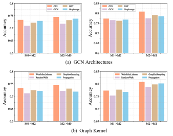
Figure 5: The performance with different GCN architectures and graph kernels on Mutagenicity.

Appendix B Introduction of Baselines

• WL subtree (Shervashidze et al., 2011): WL subtree is a kernel method, which measures the similarity between graphs with the defined kernel function.

• GCN (Kipf & Welling, 2017): The main idea of GCN is to combine neighborhood information to update each central node, so as to obtain a representation vector in an iterative fashion.

• GIN (Xu et al., 2019): GIN is a well-known message passing neural networks with improved expressive capability.

• CIN (Bodnar et al., 2021): CIN extends the theoretical results on Simplicial Complexes to regular Cell Complexes, which achieves a better performance.

• GMT (Baek et al., 2021): GMT is a multi-head attention-based model, which captures interactions between nodes according to their structural dependencies.

• CDAN (Long et al., 2018): CDAN utilizes a adversarial adaptation framework conditioned on discriminative information extracted from the predictions of the classifier.

• ToAlign (Wei et al., 2021b): ToAlign aims to align the domain by performing feature decomposition and the prior knowledge including classification task itself.

• MetaAlign (Wei et al., 2021a): MetaAlign separates the domain alignment and the classification objectives as two individual tasks, i.e., meta-train and meta-test, and uses a meta-optimization method to optimize these two tasks.

• DUA (Mirza et al., 2022): DUA proposes an effective normalization technique for domain adaptation.

Appendix C Additional Experiments

We conduct more experiments to evaluate the effect of different GCN architectures and Graph kernels. Figure 5 shows the performance of different GCN architectures and graph kernels on Mutagenicity. From Figure 5, we have the similarity observations as described in Section 4.3, validating the effectiveness of GIN and WL kernel once again.

References

- Assran et al. (2021) Assran, M., Caron, M., Misra, I., Bojanowski, P., Joulin, A., Ballas, N., and Rabbat, M. Semi-supervised learning of visual features by non-parametrically predicting view assignments with support samples. In ICCV, pp. 8443–8452, 2021.
- Baek et al. (2021) Baek, J., Kang, M., and Hwang, S. J. Accurate learning of graph representations with graph multiset pooling. In ICLR, 2021.
- Bodnar et al. (2021) Bodnar, C., Frasca, F., Otter, N., Wang, Y. G., Liò, P., Montufar, G. F., and Bronstein, M. Weisfeiler and lehman go cellular: Cw networks. In NeurIPS, pp. 2625–2640, 2021.
- Borgwardt & Kriegel (2005) Borgwardt, K. M. and Kriegel, H.-P. Shortest-path kernels on graphs. In ICDM, 2005.
- Chen et al. (2020a) Chen, D., Jacob, L., and Mairal, J. Convolutional kernel networks for graph-structured data. In ICML, pp. 1576–1586, 2020a.
- Chen et al. (2020b) Chen, T., Kornblith, S., Norouzi, M., and Hinton, G. A simple framework for contrastive learning of visual representations. In ICML, 2020b.
- Cosmo et al. (2021) Cosmo, L., Minello, G., Bronstein, M., Rodolà, E., Rossi, L., and Torsello, A. Graph kernel neural networks. arXiv preprint arXiv:2112.07436, 2021.
- Dobson & Doig (2003) Dobson, P. D. and Doig, A. J. Distinguishing enzyme structures from non-enzymes without alignments. Journal of molecular biology, 330(4):771–783, 2003.
- Fan et al. (2019) Fan, W., Ma, Y., Li, Q., He, Y., Zhao, E., Tang, J., and Yin, D. Graph neural networks for social recommendation. In WWW, pp. 417–426, 2019.
- Feng et al. (2022) Feng, A., You, C., Wang, S., and Tassiulas, L. Kergnns: Interpretable graph neural networks with graph kernels. In AAAI, 2022.
- Ganin et al. (2016) Ganin, Y., Ustinova, E., Ajakan, H., Germain, P., Larochelle, H., Laviolette, F., Marchand, M., and Lempitsky, V. Domain-adversarial training of neural networks. Journal of Machine Learning Research, 17(1):2096–2030, 2016.
- Gilmer et al. (2017) Gilmer, J., Schoenholz, S. S., Riley, P. F., Vinyals, O., and Dahl, G. E. Neural message passing for quantum chemistry. In ICML, 2017.
- Gresele et al. (2020) Gresele, L., Fissore, G., Javaloy, A., Schölkopf, B., and Hyvarinen, A. Relative gradient optimization of the jacobian term in unsupervised deep learning. 2020.
- Hamilton et al. (2017) Hamilton, W. L., Ying, R., and Leskovec, J. Inductive representation learning on large graphs. In NeurIPS, 2017.
- Hassani (2022) Hassani, K. Cross-domain few-shot graph classification. In AAAI, 2022.
- He et al. (2020) He, K., Fan, H., Wu, Y., Xie, S., and Girshick, R. Momentum contrast for unsupervised visual representation learning. In CVPR, 2020.
- He et al. (2022) He, T., Shen, L., Guo, Y., Ding, G., and Guo, Z. Secret: Self-consistent pseudo label refinement for unsupervised domain adaptive person re-identification. In AAAI, 2022.
- Huang et al. (2021) Huang, J., Guan, D., Xiao, A., and Lu, S. Model adaptation: Historical contrastive learning for unsupervised domain adaptation without source data. In NeurIPS, pp. 3635–3649, 2021.
- Huang et al. (2022) Huang, J., Guan, D., Xiao, A., Lu, S., and Shao, L. Category contrast for unsupervised domain adaptation in visual tasks. In CVPR, 2022.
- Ju et al. (2022) Ju, W., Gu, Y., Chen, B., Sun, G., Qin, Y., Liu, X., Luo, X., and Zhang, M. Glcc: A general framework for graph-level clustering. arXiv preprint arXiv:2210.11879, 2022.
- Ju et al. (2023a) Ju, W., Fang, Z., Gu, Y., Liu, Z., Long, Q., Qiao, Z., Qin, Y., Shen, J., Sun, F., Xiao, Z., et al. A comprehensive survey on deep graph representation learning. arXiv preprint arXiv:2304.05055, 2023a.
- Ju et al. (2023b) Ju, W., Luo, X., Qu, M., Wang, Y., Chen, C., Deng, M., Hua, X.-S., and Zhang, M. Tgnn: A joint semi-supervised framework for graph-level classification. arXiv preprint arXiv:2304.11688, 2023b.
- Kalofolias et al. (2021) Kalofolias, J., Welke, P., and Vreeken, J. Susan: The structural similarity random walk kernel. In SDM, 2021.
- Kang et al. (2012) Kang, U., Tong, H., and Sun, J. Fast random walk graph kernel. In SDM, 2012.
- Kazius et al. (2005) Kazius, J., McGuire, R., and Bursi, R. Derivation and validation of toxicophores for mutagenicity prediction. Journal of medicinal chemistry, 48(1):312–320, 2005.
- Khosla et al. (2020) Khosla, P., Teterwak, P., Wang, C., Sarna, A., Tian, Y., Isola, P., Maschinot, A., Liu, C., and Krishnan, D. Supervised contrastive learning. In NeurIPS, pp. 18661–18673, 2020.
- Kipf & Welling (2017) Kipf, T. N. and Welling, M. Semi-supervised classification with graph convolutional networks. In ICLR, 2017.
- Kong et al. (2022) Kong, K., Li, G., Ding, M., Wu, Z., Zhu, C., Ghanem, B., Taylor, G., and Goldstein, T. Robust optimization as data augmentation for large-scale graphs. In CVPR, 2022.
- Kundu et al. (2022) Kundu, J. N., Kulkarni, A. R., Bhambri, S., Jampani, V., and Radhakrishnan, V. B. Amplitude spectrum transformation for open compound domain adaptive semantic segmentation. In AAAI, 2022.
- Lee et al. (2013) Lee, D.-H. et al. Pseudo-label: The simple and efficient semi-supervised learning method for deep neural networks. In ICMLW, 2013.
- Lee et al. (2019) Lee, J., Lee, I., and Kang, J. Self-attention graph pooling. In ICML, 2019.
- Leskovec & Faloutsos (2006) Leskovec, J. and Faloutsos, C. Sampling from large graphs. In KDD, 2006.
- Li et al. (2020) Li, J., Zhou, P., Xiong, C., and Hoi, S. C. Prototypical contrastive learning of unsupervised representations. arXiv preprint arXiv:2005.04966, 2020.
- Liang et al. (2020) Liang, J., Hu, D., and Feng, J. Do we really need to access the source data? source hypothesis transfer for unsupervised domain adaptation. In ICML, 2020.
- Liao et al. (2021) Liao, S., Liang, S., Meng, Z., and Zhang, Q. Learning dynamic embeddings for temporal knowledge graphs. In WSDM, 2021.
- Long et al. (2015) Long, M., Cao, Y., Wang, J., and Jordan, M. Learning transferable features with deep adaptation networks. In ICML, 2015.
- Long et al. (2018) Long, M., Cao, Z., Wang, J., and Jordan, M. I. Conditional adversarial domain adaptation. In NeurIPS, 2018.
- Long et al. (2021) Long, Q., Jin, Y., Wu, Y., and Song, G. Theoretically improving graph neural networks via anonymous walk graph kernels. In WWW, 2021.
- Mirza et al. (2022) Mirza, M. J., Micorek, J., Possegger, H., and Bischof, H. The norm must go on: Dynamic unsupervised domain adaptation by normalization. In CVPR, 2022.
- Morris et al. (2020) Morris, C., Kriege, N. M., Bause, F., Kersting, K., Mutzel, P., and Neumann, M. Tudataset: A collection of benchmark datasets for learning with graphs. In ICMLW, 2020.
- Neumann et al. (2016) Neumann, M., Garnett, R., Bauckhage, C., and Kersting, K. Propagation kernels: efficient graph kernels from propagated information. Machine Learning, 102(2):209–245, 2016.
- Nguyen et al. (2022) Nguyen, A. T., Tran, T., Gal, Y., Torr, P. H., and Baydin, A. G. Kl guided domain adaptation. In ICLR, 2022.
- Passalis & Tefas (2018) Passalis, N. and Tefas, A. Training lightweight deep convolutional neural networks using bag-of-features pooling. IEEE Transactions on Neural Networks and Learning Systems, 30(6):1705–1715, 2018.
- Qiu et al. (2021) Qiu, Z., Su, Q., Ou, Z., Yu, J., and Chen, C. Unsupervised hashing with contrastive information bottleneck. In IJCAI, 2021.
- Schulz & Welke (2019) Schulz, T. and Welke, P. On the necessity of graph kernel baselines. In ECML-PKDD, GEM workshop, 2019.
- Sharma et al. (2016) Sharma, A., Boroevich, K. A., Shigemizu, D., Kamatani, Y., Kubo, M., and Tsunoda, T. Hierarchical maximum likelihood clustering approach. IEEE Transactions on Biomedical Engineering, 64(1):112–122, 2016.
- Shen et al. (2018) Shen, J., Qu, Y., Zhang, W., and Yu, Y. Wasserstein distance guided representation learning for domain adaptation. In AAAI, 2018.
- Shervashidze et al. (2009) Shervashidze, N., Vishwanathan, S., Petri, T., Mehlhorn, K., and Borgwardt, K. Efficient graphlet kernels for large graph comparison. In AISTATS, 2009.
- Shervashidze et al. (2011) Shervashidze, N., Schweitzer, P., Van Leeuwen, E. J., Mehlhorn, K., and Borgwardt, K. M. Weisfeiler-lehman graph kernels. Journal of Machine Learning Research, 12(9):2539–2561, 2011.
- Song et al. (2016) Song, G., Li, Y., Chen, X., He, X., and Tang, J. Influential node tracking on dynamic social network: An interchange greedy approach. IEEE Transactions on Knowledge and Data Engineering, 29(2):359–372, 2016.
- Suresh et al. (2021) Suresh, S., Li, P., Hao, C., and Neville, J. Adversarial graph augmentation to improve graph contrastive learning. In NeurIPS, 2021.
- Sutherland et al. (2003) Sutherland, J. J., O’brien, L. A., and Weaver, D. F. Spline-fitting with a genetic algorithm: A method for developing classification structure- activity relationships. Journal of Chemical Information and Computer Sciences, 2003.
- Tan et al. (2020) Tan, Q., Liu, N., Zhao, X., Yang, H., Zhou, J., and Hu, X. Learning to hash with graph neural networks for recommender systems. In WWW, 2020.
- Veličković et al. (2018) Veličković, P., Cucurull, G., Casanova, A., Romero, A., Liò, P., and Bengio, Y. Graph Attention Networks. ICLR, 2018.
- Wang et al. (2022) Wang, R., Wu, Z., Weng, Z., Chen, J., Qi, G.-J., and Jiang, Y.-G. Cross-domain contrastive learning for unsupervised domain adaptation. IEEE Transactions on Multimedia, 2022.
- Wang et al. (2021) Wang, Y., Wang, W., Liang, Y., Cai, Y., and Hooi, B. Mixup for node and graph classification. In WWW, pp. 3663–3674, 2021.
- Wei et al. (2021a) Wei, G., Lan, C., Zeng, W., and Chen, Z. Metaalign: Coordinating domain alignment and classification for unsupervised domain adaptation. In CVPR, 2021a.
- Wei et al. (2021b) Wei, G., Lan, C., Zeng, W., Zhang, Z., and Chen, Z. Toalign: Task-oriented alignment for unsupervised domain adaptation. In NeurIPS, 2021b.
- Wu et al. (2020a) Wu, M., Pan, S., Zhou, C., Chang, X., and Zhu, X. Unsupervised domain adaptive graph convolutional networks. In WWW, 2020a.
- Wu et al. (2020b) Wu, Z., Pan, S., Chen, F., Long, G., Zhang, C., and Philip, S. Y. A comprehensive survey on graph neural networks. IEEE Transactions on Neural Networks and Learning Systems, 32(1):4–24, 2020b.
- Xiao & Zhang (2021) Xiao, N. and Zhang, L. Dynamic weighted learning for unsupervised domain adaptation. In CVPR, 2021.
- Xu et al. (2021) Xu, D., Cheng, W., Luo, D., Chen, H., and Zhang, X. Infogcl: Information-aware graph contrastive learning. In NeurIPS, 2021.
- Xu et al. (2019) Xu, K., Hu, W., Leskovec, J., and Jegelka, S. How powerful are graph neural networks? In ICLR, 2019.
- Yang et al. (2022) Yang, H., Chen, H., Pan, S., Li, L., Yu, P. S., and Xu, G. Dual space graph contrastive learning. In WWW, pp. 1238–1247, 2022.
- Yin et al. (2022a) Yin, N., Shen, L., Li, B., Wang, M., Luo, X., Chen, C., Luo, Z., and Hua, X.-S. Deal: An unsupervised domain adaptive framework for graph-level classification. In ACMMM, pp. 3470–3479, 2022a.
- Yin et al. (2022b) Yin, Y., Wang, Q., Huang, S., Xiong, H., and Zhang, X. Autogcl: Automated graph contrastive learning via learnable view generators. In AAAI, 2022b.
- Yoo et al. (2022) Yoo, J., Shim, S., and Kang, U. Model-agnostic augmentation for accurate graph classification. In WWW, 2022.
- You et al. (2020) You, Y., Chen, T., Sui, Y., Chen, T., Wang, Z., and Shen, Y. Graph contrastive learning with augmentations. 2020.
- You et al. (2021) You, Y., Chen, T., Shen, Y., and Wang, Z. Graph contrastive learning automated. In ICML, 2021.
- Zhang et al. (2021) Zhang, T., Wang, Y., Cui, Z., Zhou, C., Cui, B., Huang, H., and Yang, J. Deep wasserstein graph discriminant learning for graph classification. In AAAI, 2021.
- Zheng et al. (2021) Zheng, K., Liu, W., He, L., Mei, T., Luo, J., and Zha, Z.-J. Group-aware label transfer for domain adaptive person re-identification. In CVPR, 2021.