Conservative Prediction via
Data-Driven Confidence Minimization

Abstract

Errors of machine learning models are costly, especially in safety-critical domains such as healthcare, where such mistakes can prevent the deployment of machine learning altogether. In these settings, conservative models – models which can defer to human judgment when they are likely to make an error – may offer a solution. However, detecting unusual or difficult examples is notably challenging, as it is impossible to anticipate all potential inputs at test time. To address this issue, prior work [22] has proposed to minimize the model’s confidence on an auxiliary pseudo-OOD dataset. We theoretically analyze the effect of confidence minimization and show that the choice of auxiliary dataset is critical. Specifically, if the auxiliary dataset includes samples from the OOD region of interest, confidence minimization provably separates ID and OOD inputs by predictive confidence. Taking inspiration from this result, we present Data-Driven Confidence Minimization (DCM), which minimizes confidence on an uncertainty dataset containing examples that the model is likely to misclassify at test time. Our experiments show that DCM consistently outperforms state-of-the-art OOD detection methods on 8 ID-OOD dataset pairs, reducing FPR (at TPR 95%) by $6.3\%$ and $58.1\%$ on CIFAR-10 and CIFAR-100, and outperforms existing selective classification approaches on 4 datasets in conditions of distribution shift.

1 Introduction

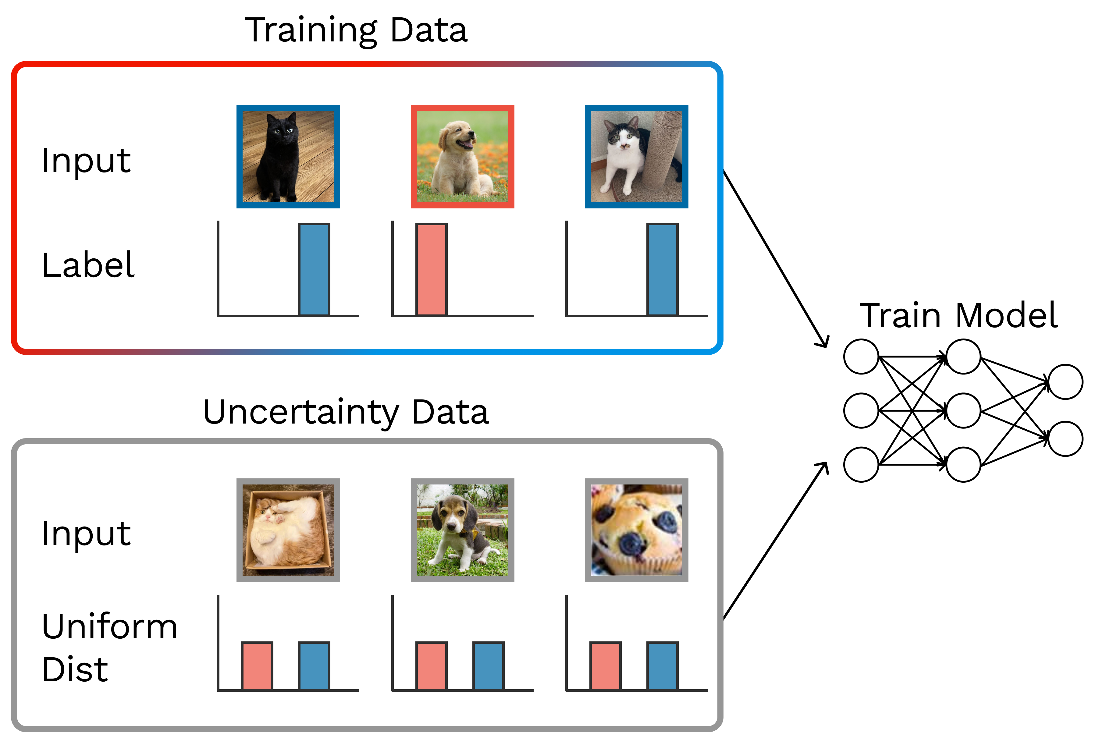
Figure 1: Visual overview of data-driven confidence minimization (DCM), our method for training a model to make conservative predictions. We minimize cross-entropy loss on labeled training data and confidence on uncertainty data.

While deep networks have demonstrated remarkable performance on many tasks, they often fail unexpectedly on inputs with high confidence [46, 57]. These errors can lead to poor performance or even catastrophic failure. In safety-critical domains such as healthcare, such errors may prevent the deployment of machine learning altogether. Conservative models—models that can refrain from making predictions when they are likely to make an error—may offer a solution. For example, a tumor detection model that is trained on histopathological images from one hospital may perform poorly when deployed in other hospitals due to differences in data collection methods or patient population [27]. In these scenarios, it may be preferable to defer to a human expert.

Despite considerable research in out-of-distribution (OOD) detection [21, 36, 34, 37] and selective classification [38, 25, 24], the problem of learning a conservative model remains challenging. Indeed, Tajwar et al. [48] observes that the performance of prior OOD detection methods is inconsistent across evaluation settings. As the test distribution can vary in a myriad of ways, it is impractical to anticipate the exact examples that will arise at test time. Any detection mechanism will itself inevitably face unfamiliar inputs, making this problem difficult without additional assumptions. In this context, a promising approach to producing a conservative model is Outlier Exposure [22], which minimizes confidence on a large, auxiliary dataset of “pseudo-OOD” examples during training. Outlier Exposure fine-tunes a pretrained model with a combined objective of the standard cross-entropy loss on in-distribution examples and an additional term that minimizes predictive confidence on the pseudo-OOD examples. Unlabeled auxiliary data is often readily available, making it an effective way of exposing the model to the types of OOD inputs it may encounter at test time.

We refer to the broader framework of minimizing confidence on an auxiliary uncertainty dataset as Data-Driven Confidence Minimization (DCM). DCM minimizes confidence on all examples in the uncertainty dataset while minimizing the standard ID training objective. Within the DCM framework, we find that the choice of uncertainty dataset is crucial: using an uncertainty dataset that more closely represents unfamiliar inputs the model may face at test time results in a better conservative model. Specifically, our theoretical analysis shows that minimizing confidence provably induces separation in confidence for in-distribution (ID) vs out-of-distribution (OOD) examples, but only for OOD examples represented in the uncertainty dataset. We introduce two new particularly effective forms of uncertainty dataset for the OOD detection and selective classification problem settings. For OOD detection, we use an uncertainty dataset consisting of unlabeled examples from the test distribution, which contains both ID and OOD inputs. This results in a model that is under-confident on only OOD inputs, because the effect of minimizing confidence on ID examples in the uncertainty dataset is “cancelled out” by the regular ID training objective. For selective classification, the uncertainty dataset consists of misclassified validation examples from the source distribution. We illustrate our approach in Figure 1.

We empirically verify our approach through experiments on several standard benchmarks for OOD detection and selective classification. Among other methods, we provide a comparison with Outlier Exposure [22], which falls within the DCM framework and uses a very large uncertainty dataset that is over $10,000$ times larger than ours. DCM consistently outperforms Outlier Exposure on a benchmark of $8$ ID-OOD distribution pairs, reducing FPR (at TPR 95%) by 6.3% and 58.1% on CIFAR-10 and CIFAR-100, respectively. DCM is also able to effectively identify OOD inputs in challenging near-OOD settings, achieving $1.89\%$ and $2.94\%$ higher AUROC compared to ERD [50], a state-of-the-art method which also uses an unlabeled exposure set. In selective classification, DCM consistently outperforms $6$ representative approaches in conditions of distribution shift, including Deep Gamblers [38] and Self-Adaptive Training [24]. DCM also outperforms an ensemble of $5$ models on $3$ out of $4$ datasets, despite the difference in computational cost. These results suggest that DCM is a promising framework for conservative prediction in safety-critical scenarios.

2 Problem Setup

We consider two problem settings that test a model’s ability to determine if its prediction is trustworthy: out-of-distribution (OOD) detection and selective classification. In both settings, we denote the input and label spaces as $\mathcal{X}$ and $\mathcal{Y}$, respectively, and assume that the training dataset $D_{\textrm{tr}}$ is drawn from the ID distribution $\mathcal{P}_{\textrm{ID}}$. In out-of-distribution detection, the model may encounter inputs that do not belong to any class in its label space $\mathcal{Y}$, such as inputs from an entirely new class. In selective classification, all inputs have a ground-truth label within $\mathcal{Y}$, but the model may make errors due to overfitting or insufficient coverage in the training dataset $D_{\textrm{tr}}$. We first describe these two problem settings. In Section 3, we present two variants of DCM for OOD detection and selective classification.

2.1 Out-of-Distribution Detection

In this problem setting, the model may encounter datapoints from a different distribution $\mathcal{P}_{\textrm{OOD}}$ at test time, and the goal is to detect such OOD inputs. The test dataset is sampled from a mixture of the ID and OOD distributions $\alpha_{\text{test}}\mathcal{P}_{\textrm{ID}}+(1-\alpha_{\text{test}})\mathcal{P}_{\textrm{OOD}}$, where the mixture coefficient $\alpha_{\text{test}}$ is not known in advance. Because of the differences in $\mathcal{P}_{\textrm{ID}}$ and $\mathcal{P}_{\textrm{OOD}}$, a model trained solely to minimize loss on $D_{\textrm{tr}}$ may be inaccurate or overconfident when tested on novel inputs from $\mathcal{P}_{\textrm{OOD}}$. To address this challenge, we incorporate an additional unlabeled test set $D_{\textrm{u}}$ that is also drawn from a mixture of $\mathcal{P}_{\textrm{ID}}$ and $\mathcal{P}_{\textrm{OOD}}$; the mixture ratio $\alpha_{\text{u}}$ is unknown to the model and can differ from $\alpha_{\text{test}}$. This unlabeled dataset partially informs the model about the directions of variation that it may face in the OOD distribution.

Given a test input $x$, the model makes a label prediction and also an estimate of confidence that should be higher for inputs that are more likely to be ID. Using the test set, we evaluate the model on two aspects: (1) whether the model’s confidence can successfully determine whether an input is OOD; and for ID inputs specifically, (2) whether the model’s prediction agrees with the ground-truth label. These capabilities are measured by metrics such as FPR@TPR, AUROC, and AUPR; we further describe these metrics, along with the specific ID-OOD dataset pairs used for empirical evaluation, in Section 6.

2.2 Selective Classification

In the selective classification setting, we aim to identify test inputs that the model should abstain from making predictions on. This problem is applicable to situations where the consequences of an incorrect classification attempt are severe, so abstaining from prediction is strongly preferred over making a potentially incorrect prediction. After training on training data $D_{\textrm{tr}}\sim\mathcal{P}_{\textrm{ID}}$, the model is tested on a test dataset sampled from a mixture of the ID and OOD distributions $\alpha\mathcal{P}_{\textrm{ID}}+(1-\alpha)\mathcal{P}_{\textrm{OOD}}$; we test the ID and OOD cases ($\alpha=1$ and $\alpha=0$) in addition to the general case ($\alpha=0.5$) in our experiments. Unlike the previous OOD detection setting, we consider more closely related OOD distributions where even the inputs from $\mathcal{P}_{\textrm{OOD}}$ have a ground-truth label within the label space $\mathcal{Y}$. While an ideal model would perfectly predict the labels of even the OOD inputs, models often make errors on new inputs—both ID and OOD—due to overfitting. As in prior work, we assume access to a labeled validation dataset $D_{\textrm{val}}$ sampled from $\mathcal{P}_{\textrm{ID}}$, which the model can use to calibrate its predictive confidence. We note that this validation set can be constructed by randomly partitioning an original training dataset into training and validation splits.

We evaluate a given model with the assumption that it can abstain from making a prediction on some test inputs. Such “rejected” inputs are typically ones that the model is most uncertain about. In this problem setting, we want a balance between two capabilities in the model: (1) the model should make accurate predictions of ground-truth labels for the inputs that it does make predictions on (i.e., accuracy), while (2) rejecting as few inputs as possible (i.e., coverage). We measure these capabilities through existing metrics such as ECE, AUC, Acc@Cov, Cov@Acc. We defer a detailed description of these metrics, along with the specific ID and OOD datasets used for empirical evaluation, in Section 6.

3 Data-Driven Confidence Minimization

We aim to produce a model that achieves high accuracy on the training data $D_{\textrm{tr}}$ while having a predictive confidence that reflects the extent to which its prediction can be trusted. The crux of the method is to introduce a regularizer that minimizes confidence on a dataset that is disjoint from the training dataset. We refer to this dataset as the “uncertainty dataset,” since it is intended to contain examples that the model should be uncertain about.

In DCM, we first pre-train a model $f:\mathcal{X}\rightarrow\mathbb{P}(\mathcal{Y})$ on the labeled training set using the standard cross-entropy loss, as in prior works [21, 22, 37]:

$$\mathcal{L}_{\text{xent}}(f,D_{\textrm{tr}})=\operatorname*{\mathbb{E}}_{(x,y)\sim D_{\textrm{tr}}}\left[-\log f(y;x)\right].$$ (1)

A model trained solely to minimize training loss can suffer from overconfidence and produce high-confidence predictions for inputs that are not represented in the training dataset $D_{\textrm{tr}}$. We therefore fine-tune this model while regularizing to minimize the predictive confidence on such inputs. More specifically, we continue to minimize cross-entropy loss on a fine-tuning dataset which includes the original training data ($D_{\textrm{tr}}\subseteq D_{\textrm{ft}}$). Our additional regularizer minimizes confidence on an “uncertainty dataset” $D_{\textrm{unc}}$; we define the corresponding regularization loss as

$$\mathcal{L}_{\text{conf}}(f,D_{\textrm{unc}})=\operatorname*{\mathbb{E}}_{x^{\prime}\sim D_{\textrm{unc}}}\left[-\log f(y_{u};x^{\prime})\right].$$ (2)

Here, $y_{u}$ is a uniform target that assigns equal probability to all labels. The confidence loss $\mathcal{L}_{\textrm{conf}}$ is equivalent to the KL divergence between the predicted probabilities and the uniform distribution $U$. Our final objective is a weighted sum of the fine-tuning and confidence losses:

$$\mathcal{L}_{\text{xent}}(f,D_{\textrm{ft}})+\lambda\mathcal{L}_{\text{conf}}(f,D_{\textrm{unc}}),$$ (3)

where $\lambda$ is a hyperparameter that controls the relative weight of the confidence loss term. We find that $\lambda=0.5$ works well in practice and use this value in all experiments unless otherwise specified. Further details (e.g. size of $D_{\text{ft}}$ and $D_{\text{unc}}$, length of fine-tuning) are described in Appendix C. The two algorithm variants for OOD detection and selective classification differ only in how they select $D_{\textrm{ft}}$ and $D_{\textrm{unc}}$, as we will see in Sections 3.1 and 3.2.

3.1 DCM for Out-of-Distribution Detection

Our goal in out-of-distribution detection is to produce a model that achieves high accuracy on the ID distribution $\mathcal{P}_{\textrm{ID}}$ while having low confidence on OOD inputs from the OOD distribution $\mathcal{P}_{\textrm{OOD}}$. Recall that our problem setting assumes access to an unlabeled dataset $D_{\textrm{u}}$, which includes both ID and OOD inputs: we use this unlabeled set as the uncertainty dataset for reducing confidence ($D_{\textrm{unc}}=D_{\textrm{u}}$). Intuitively, minimizing confidence loss on $D_{\textrm{u}}$ discourages the model from making overly confident predictions on the support of the uncertainty dataset.

We minimize confidence on all inputs in $D_{\textrm{u}}$ because it is not known a priori which inputs are ID versus OOD. While we do not necessarily want to minimize confidence on ID inputs, this confidence minimization is expected to have different effects on ID and OOD inputs because of its interaction with the original cross-entropy loss. On ID inputs, the effect of minimizing confidence is “averaged out” by the cross-entropy loss because maximizing the log likelihood of the true label entails increasing the predictive confidence for that input. However, on OOD inputs, the confidence loss is the sole loss term, which forces the model to have low confidence on OOD inputs. This allows DCM to differentiate between the ID and OOD data distributions based on predictive confidence.

In summary, in the OOD detection setting, the fine-tuning dataset is the training dataset ($D_{\textrm{ft}}=D_{\textrm{tr}}$), and the uncertainty dataset is the unlabeled dataset ($D_{\textrm{unc}}=D_{\textrm{u}}$). We outline our approach in Algorithm 1.

  Input: Training data $D_{\textrm{tr}}$, Unlabeled data $D_{\textrm{u}}$, Hyperparamter $\lambda$

  Initialize weights $\theta\leftarrow\theta_{0}$

  while Not converged do

    Sample mini-batch $B_{\textrm{tr}}\sim D_{\textrm{tr}}$

    Update $\theta$ using $\nabla_{\theta}\mathcal{L}_{\textrm{xent}}(f,B_{\textrm{tr}})$

  end while

  while Not converged do

    Sample mini-batches $B_{\textrm{tr}}\sim D_{\textrm{tr}},B_{\textrm{u}}\sim D_{\textrm{u}}$

    Update $\theta$ using $\nabla_{\theta}\mathcal{L}_{\textrm{xent}}(f,B_{\textrm{tr}})+\lambda\mathcal{L}_{\textrm{conf}}(f,B_{\textrm{u}})$

  end while

Algorithm 1 DCM for OOD Detection

  Input: Training data $D_{\textrm{tr}}$, Validation data $D_{\textrm{val}}$, Hyperparameter $\lambda$

  Initialize weights $\theta\leftarrow\theta_{0}$

  while Not converged do

    Sample mini-batch $B_{\textrm{tr}}\sim D_{\textrm{tr}}$

    Update $\theta$ using $\nabla_{\theta}\mathcal{L}_{\textrm{xent}}(B_{\textrm{tr}},f)$

  end while

  Get correct set $D_{\textrm{val}}^{\circ}\leftarrow\{(x,y)\in D_{\textrm{val}}\mid f_{\theta}(x)=y\}$

  Get error set $D_{\textrm{val}}^{\times}\leftarrow\{(x,y)\in D_{\textrm{val}}\mid f_{\theta}(x)\neq y\}$

  while Not converged do

    Sample mini-batches $B_{\textrm{tr}}\sim D_{\textrm{tr}}\cup D_{\textrm{val}}^{\circ},B_{\textrm{val}}^{\times}\sim D_{\textrm{val}}^{\times}$

    Update $\theta$ using $\nabla_{\theta}\mathcal{L}_{\textrm{xent}}(B_{\textrm{tr}},f)+\lambda\mathcal{L}_{\textrm{conf}}(B_{\textrm{val}}^{\times},f)$

  end while

Algorithm 2 DCM for Selective Classification

3.2 DCM for Selective Classification

As described in Section 2, in the selective classification setting, we aim to produce a model that achieves high accuracy while having low confidence on inputs it is likely to misclassify. After training a model $f$ on the training data, we expect its errors on the held-out validation set to reflect the failure modes of the original model. Recall that we assume a held-out validation set $D_{\textrm{val}}\sim\mathcal{P}_{\textrm{ID}}$. To better calibrate its predictive confidence, we compare our pre-trained model’s predictions for inputs in $D_{\textrm{val}}$ to their ground-truth labels, and obtain the set of correct and misclassified validation examples $D_{\textrm{val}}^{\circ},D_{\textrm{val}}^{\times}$. The misclassified example set $D_{\textrm{val}}^{\times}$ shows where the model’s decision boundary conflicts with the true labeling function.

We set the fine-tuning dataset to be the union of the training dataset and the correct validation examples ($D_{\textrm{ft}}=D_{\textrm{tr}}\cup D_{\textrm{val}}^{\circ}$), and use the misclassified validation examples as the uncertainty dataset ($D_{\textrm{unc}}=D_{\textrm{val}}^{\times}$). By minimizing confidence on only the misclassified examples, we expect the model to have lower confidence on all examples which share commonalities with samples which initially produced errors. We outline our approach in Algorithm 2.

4 Analysis

We now theoretically analyze the effect of the DCM objective on ID and OOD inputs. We first show that for all test examples, the prediction confidence of DCM is a lower bound on the true confidence (Proposition 4.1). Using this property, we then demonstrate that DCM can provably detect OOD examples by thresholding the predicted confidence (Proposition 4.2). Detailed statements and proofs can be found in Appendix A.

We denote the true label distribution of input $x$ as $p_{D}(x)$; this distribution need not be a point mass on a single label. We further denote the maximum softmax probability of any distribution $p$ as $\textrm{MSP}(p)\triangleq\max_{i}p_{i}$, and denote by $f_{\lambda}(x)$ the predictive distribution of the model that minimizes the expectation of our objective 3 with respect to the data distribution $y\sim p_{D}(x)$ for input $x$. Intuitively, the confidence minimization term in our objective function 3 forces the model to output low-confidence predictions on all datapoints, resulting in a more conservative model compared to one without this term. We formalize this intuition in the following proposition which relates the maximum softmax probabilities of $f_{\lambda}$ and $p_{D}$.

Proposition 4.1 (Lower bound on true confidence).

For any input $x$ in $D_{u}$ or the support of $\mathcal{P}_{\textrm{ID}}$, the optimal predictive distribution $f_{\lambda}$ satisfies $\textrm{MSP}(f_{\lambda})\leq\textrm{MSP}(p_{D})$, with equality if and only if $\lambda=0$.

We note that this proposition only assumes a sufficiently expressive model class (which large neural networks often are).

Beyond serving as a lower bound on the true confidence, the optimum distribution $p_{\lambda}$ shows how the model behaves differently for ID and OOD data, despite the unlabeled dataset $D_{\textrm{u}}$ containing both. We denote the subset of ID examples in $D_{\textrm{u}}$ as $D^{test}_{in}$, the OOD subset as $D^{test}_{out}$, and the $\delta$-neighborhoods of these two sets as $D^{\delta}_{in},D^{\delta}_{out}$. For ID inputs, the optimal predictive distribution $p_{\lambda}$ is determined by the weighted sum of the cross-entropy loss and the confidence loss, resulting in a mixture between the true label distribution $p$ and the uniform distribution $\mathcal{U}$, with mixture weight $\lambda$. On the other hand, for OOD inputs, the confidence loss is the only loss term, thus the optimal predictive distribution $p_{\lambda}$ is the uniform distribution $\mathcal{U}$. This distinct behavior allows for the detection of OOD inputs by thresholding the confidence of the model’s predictions, as formalized in the following proposition.

Proposition 4.2 (Low loss implies separation).

Assume $D^{\delta}_{in}$ and $D^{\delta}_{out}$ are disjoint, and that each input $x$ has only one ground-truth label, i.e., no label noise. Denote the lowest achievable loss for the objective with $\lambda>0$ as $\mathcal{L}_{0}$. Under a mild smoothness assumption on the learned function $f_{\theta}$, there exists $\epsilon,\delta>0$ such that $\mathcal{L}(\theta)-\mathcal{L}_{0}<\epsilon$ implies the following relationship between the max probabilities:

$$\inf_{x\in D^{\delta}_{in}}\textrm{MSP}(f_{\theta}^{i}(x))>\sup_{x\in D^{\delta}_{out}}\textrm{MSP}(f_{\theta}^{i}(x)).$$ (4)

The detailed smoothness assumption, along with all proofs, can be found in Appendix A. This proposition implies that by minimizing the DCM objective 3, we can provably separate out ID and OOD data with an appropriate threshold on the maximum softmax probability. We note that DCM optimizes a lower bound on confidence, rather than trying to be perfectly calibrated: this easier requirement is arguably better suited for problem settings in which the model abstains from making predictions such as OOD detection and selective classification. In Section 6, we will empirically evaluate DCM.

		ID Dataset
		CIFAR-10		CIFAR-100
Method	Architecture	AUROC ($\uparrow$)	FPR@95 ($\downarrow$)	AUROC ($\uparrow$)	FPR@95 ($\downarrow$)
MSP	WRN-40-2	90.7	30.9	70.3	72.1
Energy Score		91.5	33.2	76.0	66.7
MaxLogit		93.5	25.5	77.7	63.5
ODIN		91.0	30.9	83.3	55.2
Mahalanobis		93.6	27.3	89.1	43.0
Outlier Exposure		98.5	6.6	81.1	59.4
Energy Fine-Tuning		99.1	3.4	81.5	59.6
DCM-Softmax (ours)		99.6	1.0	99.2	2.6
DCM-MaxLogit (ours)		99.8	0.7	99.4	1.7
DCM-Energy (ours)		99.7	0.3	99.5	1.3
Binary Classifier	ResNet-18	98.9	1.3	97.9	7.6
ERD		99.5∗	1.0∗	99.1∗	2.6∗
DCM-Softmax (ours)		99.5	1.9	99.1	4.6
DCM-MaxLogit (ours)		99.5	1.5	99.2	3.5
DCM-Energy (ours)		99.5	1.4	99.3	2.3

^∗ ERD requires $3\times$ the compute compared to other methods.

Table 1: OOD detection performance of models trained on CIFAR-10 or CIFAR-100 and evaluated on 4 OOD datasets. Metrics are averaged over OOD datasets; detailed dataset-specific results are in Table 4. The three variants of DCM exhibit competitive performance on all datasets.

Setting	Method	FPR@95 ($\downarrow$)	FPR@99 ($\downarrow$)	AUROC ($\uparrow$)	AUPR ($\uparrow$)
ID = CIFAR-10 [0:5] OOD = CIFAR-10 [5:10]	Binary Classifier	92.8 (1.1)	97.8 (0.3)	55.0 (1.9)	19.7 (1.0)
	ERD	72.5 (1.7)	92.1 (0.8)	79.3 (0.3)	47.9 (1.6)
	DCM-Softmax (ours)	66.0 (2.6)	89.2 (1.0)	81.2 (0.3)	45.7 (0.6)
	DCM-MaxLogit (ours)	67.6 (5.6)	89.2 (2.2)	81.3 (0.6)	46.1 (1.4)
	DCM-Energy (ours)	67.3 (2.7)	89.1 (0.9)	81.4 (0.6)	46.3 (0.7)
ID = CIFAR-100 [0:50] OOD = CIFAR-100 [50:100]	Binary Classifier	89.0 (5.2)	92.5 (5.9)	51.4 (1.3)	17.7 (0.8)
	ERD	75.4 (0.9)	88.8 (0.5)	71.3 (0.3)	30.2 (0.5)
	DCM-Softmax (ours)	67.3 (0.5)	86.3 (0.6)	74.3 (0.2)	32.1 (0.8)
	DCM-MaxLogit (ours)	66.7 (1.5)	87.6 (2.5)	74.3 (0.5)	32.2 (1.7)
	DCM-Energy (ours)	66.7 (0.5)	87.6 (1.1)	73.9 (0.2)	32.1 (0.6)

Table 2: Near-OOD detection of ResNet-18 models on the CIFAR-10 and CIFAR-100 datasets. Numbers in parentheses represent the standard error over 5 seeds. DCM achieves comparable performance with only $1/3$ the compute of ERD.

5 Related Work

Out-of-distribution detection. Many existing methods for OOD detection use a criterion based on the activations or predictions of a model trained on ID data [2, 21, 35, 34, 53, 47]. However, the performance of these methods are often inconsistent across different ID-OOD dataset pairs, suggesting that the OOD detection problem is ill-defined  [48]. Indeed, a separate line of work incorporates auxiliary data into the OOD detection setting; this dataset may consist of natural [22, 37, 39, 49, 5, 26] or synthetic [33, 11] data. Similar to our method, Hendrycks et al. [22] minimize confidence on an auxiliary dataset, but do so on a single auxiliary dataset of known outliers, regardless of the ID and OOD distributions, that is over $10,000$ times the size of those used by DCM. Our method leverages an uncertainty dataset which contains a mix of ID and OOD data from the test distribution, as in Ţifrea et al. [49]. However, their method requires an ensemble of models to measure disagreement, while DCM uses a single model. We additionally present theoretical results showing the benefit of minimizing confidence on an uncertainty dataset that includes inputs from the OOD distribution. Our experiments confirm our theory, showing that this transductive setting results in substantial performance gains, even when the unlabeled set is a mixture of ID and OOD data.

Selective classification. Prior works have studied selective classification for many model classes including SVM, boosting, and nearest neighbors [19, 14, 7]. Because deep neural networks generalize well but are often overconfident [17, 41], mitigating such overconfidence using selective classification while preserving its generalization properties is an important capability [16, 6, 12, 25, 13]. Existing methods for learning conservative neural networks rely on additional assumptions such as pseudo-labeling [4], multiple distinct validation sets [15], or adversarial OOD examples [45]. While minimizing the confidence of a set that includes OOD inputs has been shown to result in a more conservative model in the offline reinforcement learning setting [30], this approach has not been validated in a supervised learning setting. DCM only requires a small validation set, and our experiments in Section 6 demonstrate that its performance is competitive with state-of-the-art methods for selective classification, especially in the more challenging setting of being tested on unseen OOD inputs.

6 Experiments

We evaluate the effectiveness of DCM for OOD detection and selective classification using several image classification datasets. Our aim is to empirically answer the following questions: (1) How does the data-driven confidence minimization loss affect the predictive confidence of the final model, and what role does the distribution of the uncertainty data play? (2) Does confidence minimization on the uncertainty dataset result in better calibration? (3) How does DCM compare to state-of-the-art methods for OOD detection and selective classification? We provide the full experimental setup and additional results in the appendix.

Metrics. Recall that the OOD detection problem involves two classification tasks: (1) a binary classification task to predict whether each example is ID or OOD, and (2) the main classification task of predicting labels of images. Similarly, the selective classification problem involves a binary classification task to predict whether the model will misclassify a given example, in addition to the main classification task with labels. To ensure a comprehensive evaluation, we consider multiple metrics, each measuring different aspects of the performance in the two steps. We group the metrics below according to their relevance to the OOD detection and selective classification settings as D and SC. Specifically, we consider the following metrics, which we define in detail in Appendix B:

1. FPR@TPR (D): probability that an ID input is misclassified as OOD, given true positive rate TPR.

2. AUROC (D): area under the receiver operator curve of the binary ID/OOD classification task.

3. AUPR (D): area under the precision-recall curve of the binary ID/OOD classification task.

4. ECE (SC): expected difference between confidence and accuracy, i.e. $\operatorname*{\mathbb{E}}[|p(\hat{y}=y\mid\hat{p}=p)-p|]$.

5. AUC (SC): area under the curve of selective classification accuracy vs coverage.

6. Acc@Cov (SC): average accuracy on the $\text{Cov}\%$ datapoints with highest confidence.

7. Cov@Acc (SC): largest fraction of data for which selective accuracy is above Acc.

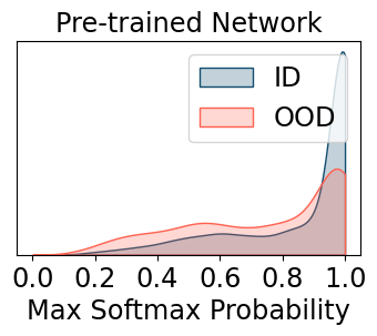
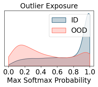
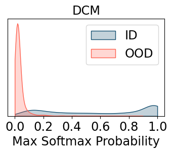
Figure 2: Distribution of maximum softmax probability for ID pre-training (left), fine-tuning with OE (middle), and fine-tuning with DCM (right). ID and OOD datasets are CIFAR-100 and TinyImageNet, respectively. DCM results in (1) better separation of predictive confidence for ID and OOD inputs, and (2) low predictive confidence on OOD inputs, suggesting that it learns a conservative model.

6.1 OOD Detection

We evaluate DCM on both the standard OOD detection setting and the more challenging near-OOD detection setting. We evaluate three variants of DCM, each using the training objective described in Section 3, but with three different measures of confidence: MSP [21], MaxLogit [23], and Energy score [37]. We denote these three variants as DCM-Softmax, DCM-MaxLogit, DCM-Energy, and describe these variants in detail in Appendix C. All experiments in this section use $\lambda=0.5$ and the default hyperparameters from Hendrycks et al. [22]. Further experimental details are in Appendix D.

Datasets. We use CIFAR-10 and CIFAR-100 as our ID datasets and TinyImageNet, LSUN, iSUN and SVHN as our OOD datasets, resulting in a total of $8$ ID-OOD pairs. We split the ID data into 40,000 examples for training and 10,000 examples for validation. Our uncertainty and test sets are disjoint datasets with 5,000 and 1,000 examples, respectively. On the near-OOD detection tasks, the ID and OOD datasets consist of disjoint classes in the same dataset (i.e., ID is the first 5 classes in CIFAR-10 and OOD is the last 5 classes.) The number of examples per class is the same as in the standard OOD detection setting.

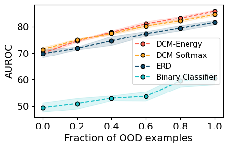
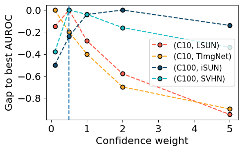
Figure 3: Robustness of DCM to hyperparameters. Left: Performance of DCM on a near-OOD detection task (CIFAR-100 [0:50] vs CIFAR-100 [50:100]) with various OOD proportions in the uncertainty dataset. Our methods, DCM-Energy and DCM-Softmax, outperform existing methods across all OOD proportions. Middle: Relative AUROC of DCM with various confidence weights $\lambda$; note the negligible differences in AUROC. Right: Selective classification performance of DCM with uncertainty datasets of various sizes on CIFAR-10 $\rightarrow$ CIFAR-10-C. These plots suggest that DCM is robust to a range of confidence weights and sizes and compositions in the uncertainty dataset.

Comparisons. In the standard OOD detection setting, we evaluate DCM against $7$ representative OOD detection methods: MSP [21], MaxLogit [23], ODIN [36], Mahalanobis [34], Energy Score [37], Outlier Exposure [22], and Energy Fine-Tuning [37]. In the more challenging near-OOD detection setting, standard methods such as Mahalanobis perform poorly  [43], so we compare DCM with Binary Classifier and ERD  [50], which attain state-of-the-art performance. Similar to DCM, these methods leverage an unlabeled dataset containing ID and OOD inputs.

DCM outperforms prior methods. For the standard OOD detection setting, we report aggregated results in Table 1 and full results in Appendix D. In this setting, DCM outperforms all 7 prior methods on all 8 ID-OOD dataset pairs, as shown in Table 1. On the more challenging near-OOD detection task, Table 2 shows that DCM outperforms Binary Classification, and performs similarly to ERD which requires $3\times$ compute. Figure 2 suggests that (1) DCM produces a conservative model that is underconfident only on OOD inputs and (2) DCM results in a better separation in predictive confidence for ID and OOD inputs than the pretrained model and Outlier Exposure.

Importance of having OOD examples in the uncertainty dataset. We analyze how the proportion of OOD data in the uncertainty dataset affects the performance of OOD detectors trained with DCM. We expect uncertainty datasets with a larger fraction of OOD examples to result in better separation, with the highest performance achieved when the uncertainty dataset consists only of OOD data. In the near-OOD detection task shown in  Figure 3, we observe improved performance with larger proportions of OOD examples in the uncertainty dataset for all methods, as expected. We note that DCM achieves the highest performance across all proportions. This indicates that the benefits from the data-driven regularization is robust to differences in uncertainty dataset composition.

DCM is robust to confidence minimization weight $\lambda$. We fix $\lambda=0.5$ for all ID-OOD dataset pairs, following the practice of Hendrycks et al. [22], DeVries & Taylor [10], Hendrycks & Gimpel [21]. While some works [33, 35] tune hyperparameters for each OOD distribution, we do not in order to test the model’s ability to detect OOD inputs from unseen distributions. We plot OOD detection performance for 4 representative ID-OOD dataset pairs with different $\lambda$ in Figure 3. While $\lambda=0.5$ is not always optimal, we find that differences in performance due to changes in $\lambda$ are negligible, suggesting that $\lambda=0.5$ is a suitable default value.

DCM still performs competitively when the uncertainty dataset is the test set itself. We report the performance of DCM using the test set as the uncertainty dataset in Table 6 and Table 7. When examples similar to those encountered at test time are not available, we find that this transductive variant of DCM still performs competitively to prior methods, despite a slight drop in performance compared to the standard DCM due to the lack of additional data.

6.2 Selective Classification

		CIFAR-10		Waterbirds		Camelyon17		FMoW
Setting	Method	Acc@90 ($\uparrow$)	AUC ($\uparrow$)	Acc@90 ($\uparrow$)	AUC ($\uparrow$)	Acc@90 ($\uparrow$)	AUC ($\uparrow$)	Acc@90 ($\uparrow$)	AUC ($\uparrow$)
ID	Ensemble ($\times 5$)	98.4 (0.1)*	99.3 (0.1)*	98.9 (0.0)*	98.7 (0.0)*	96.8 (5.9)*	99.1 (2.7)*	68.4 (0.1)*	85.5 (0.0)*
	MSP	98.4 (0.1)	99.3 (0.1)	99.1 (0.0)	98.7 (0.0)	92.0 (5.9)	96.9 (2.2)	62.6 (0.1)	81.3 (0.4)
	MaxLogit	97.9 (0.1)	98.9 (0.1)	97.2 (0.0)	98.6 (0.0)	92.2 (5.8)	97.0 (2.2)	62.7 (0.2)	80.1 (0.2)
	Binary Classifier	98.4 (0.1)	99.3 (0.1)	99.1 (0.0)	98.7 (0.0)	92.3 (5.9)	97.0 (4.5)	64.3 (0.1)	82.3 (0.3)
	Fine-Tuning	99.1 (0.2)	99.6 (0.1)	99.4 (0.0)	98.7 (0.0)	99.7 (0.0)	99.8 (0.0)	64.0 (1.2)	82.8 (0.9)
	Deep Gamblers	97.4 (0.1)	99.0 (0.0)	98.8 (0.1)	98.5 (0.0)	99.6 (0.1)	99.8 (0.0)	62.4 (0.9)	75.8 (0.2)
	Self-Adaptive Training ​​​​	97.6 (0.1)	99.2 (0.0)	99.1 (0.1)	98.6 (0.0)	99.7 (0.0)	99.8 (0.0)	63.0 (0.5)	81.1 (0.3)
	DCM (ours)	98.0 (0.2)	99.2 (0.0)	99.2 (0.0)	98.7 (0.0)	98.6 (0.2)	99.5 (0.1)	64.2 (1.2)	82.9 (1.1)
ID + OOD	Ensemble ($\times 5$)	80.6 (0.1)*	92.6 (0.1)*	–	–	78.1 (4.8)*	85.8 (3.7)*	61.2 (0.0)*	81.7 (0.0)*
	MSP	80.3 (0.1)	92.6 (0.1)	–	–	74.1 (5.1)	72.2 (4.8)	57.9 (0.1)	77.1 (0.5)
	MaxLogit	80.4 (0.0)	91.7 (0.0)	–	–	74.2 (5.1)	85.8 (3.7)	57.8 (0.1)	75.8 (0.1)
	Binary Classifier	80.3 (0.1)	92.5 (0.1)	–	–	74.4 (5.0)	86.2 (3.3)	59.3 (0.0)	78.0 (0.4)
	Fine-Tuning	81.3 (0.1)	93.4 (0.1)	–	–	79.8 (3.5)	77.6 (3.3)	58.6 (1.2)	78.6 (0.8)
	Deep Gamblers	81.0 (0.0)	93.0 (0.1)	–	–	77.2 (6.5)	88.1 (4.1)	57.5 (0.3)	71.6 (0.2)
	Self-Adaptive Training ​​​​	81.1 (0.0)	93.3 (0.0)	–	–	74.8 (1.1)	86.3 (0.4)	57.8 (0.4)	76.7 (0.2)
	DCM (ours)	82.0 (0.1)	93.6 (0.1)	–	–	85.5 (1.0)	93.5 (0.6)	58.8 (1.3)	78.9 (1.1)
OOD	Ensemble ($\times 5$)	59.8 (0.1)*	72.9 (0.1)*	88.4 (0.0)*	94.4 (0.0)*	74.0 (5.2)*	81.4 (4.4)*	58.6 (0.1)*	79.5 (0.0)*
	MSP	59.6 (0.2)	70.1 (0.1)	88.2 (0.0)	94.4 (0.0)	70.4 (4.8)	82.2 (3.9)	55.2 (0.2)	74.5 (0.6)
	MaxLogit	59.4 (0.1)	71.7 (0.1)	87.9 (0.0)	94.2 (0.0)	70.4 (4.8)	82.1 (3.9)	55.2 (0.0)	73.3 (0.2)
	Binary Classifier	59.5 (0.2)	72.8 (0.2)	87.5 (0.3)	94.0 (0.2)	70.5 (4.4)	82.4 (3.9)	56.8 (0.1)	75.6 (0.5)
	Fine-Tuning	61.9 (0.2)	75.4 (0.1)	89.0 (0.5)	94.7 (0.2)	75.4 (4.2)	84.2 (3.8)	56.0 (0.9)	76.2 (0.8)
	Deep Gamblers	61.4 (0.1)	74.3 (0.2)	88.6 (0.2)	94.8 (0.1)	72.1 (7.9)	84.8 (5.2)	54.9 (0.2)	69.2 (0.3)
	Self-Adaptive Training ​​​​	61.4 (0.1)	75.3 (0.1)	88.9 (0.1)	95.1 (0.0)	71.9 (0.8)	80.3 (0.6)	55.1 (0.4)	74.1 (0.2)
	DCM (ours)	64.1 (0.2)	77.5 (0.2)	89.5 (0.3)	95.0 (0.1)	82.5 (1.2)	91.6 (1.1)	56.2 (1.4)	76.4 (1.1)

^∗ Ensemble requires $5\times$ the compute compared to other methods.

Table 3: Selective classification performance on four datasets. Numbers in parentheses represent the standard error over $3$ seeds, and we bold all methods that have overlapping error with the best-performing method. DCM consistently achieves the best performance in settings with distribution shift (ID+OOD, OOD).

We assess the capability of models fine-tuned with DCM to abstain from making incorrect predictions. We evaluate on several toy and real-world image classification datasets that exhibit distribution shift.

Datasets. We evaluate selective classification performance on CIFAR-10 [28] and CIFAR-10-C [20], Waterbirds [44, 52], Camelyon17 [27], and FMoW [27]. These datasets were chosen to evaluate selective classification performance in the presence of diverse distribution shifts: corrupted inputs in CIFAR-10-C, spurious correlations in Waterbirds, and new domains in Camelyon17 and FMoW.

The specific ID/OOD settings for each dataset are as follows. For CIFAR-10, the ID dataset is CIFAR-10 and the OOD dataset is CIFAR-10-C. The ID+OOD dataset is a 50-50 mix of the two datasets. For Waterbirds, the ID dataset is the training split and the OOD dataset is a group-balanced validation set; we do not consider an ID+OOD dataset here. For Camelyon17, the ID dataset consists of images from the first $3$ hospitals, which are represented in the training data. The OOD dataset consists of images from the last $2$ hospitals, which do not appear in the training set. The ID+OOD dataset is a mix of all five hospitals. For FMoW, the ID dataset consists of images collected from the years $2002-2013$, which are represented in the training data. The OOD setting tests on images collected between $2016-2018$, and the ID + OOD setting tests on images from $2002-2013$ and $2016-2018$.

Comparisons. As points of comparison, we consider $6$ representative prior methods which have been shown to perform well on selective classification benchmarks: MSP [21], MaxLogit [23], Binary Classifier [25], Fine-Tuning on the labeled ID validation set, Deep Gamblers [38], and Self-Adaptive Training [24]. We also evaluate Ensemble [31], an ensemble of $5$ MSP models as a rough upper bound on performance given more compute. All methods use the same labeled ID validation set for hyperparameter tuning and/or calibration.

DCM outperforms other methods when OOD data is present. We present representative metrics in Table 3 and complete tables with all metrics in Tables 8, 9 and 10. DCM consistently outperforms all baselines in settings of distribution shift (OOD and ID+OOD). DCM even outperforms Ensemble on three of the four datasets, despite requiring $1/5$ of the compute. Fine-Tuning outperforms DCM when the training and validation datasets are from the same distribution (ID). In settings where the test distribution differs from the training and validation distributions, DCM outperforms Fine-Tuning on most metrics. These experiments indicate that the model learned by DCM is more meaningfully conservative in conditions of distribution shift, compared to state-of-the-art methods for uncertainty quantification and selective classification.

7 Conclusion

In this work, we propose Data-Driven Confidence Minimization (DCM), which trains models to make conservative predictions by minimizing confidence on an uncertainty dataset. Our empirical results demonstrate that DCM can lead to more robust classifiers, particularly in conditions of distribution shift. In our experiments, DCM consistently outperformed state-of-the-art methods for OOD detection and selective classification. We believe that the theoretical guarantees and strong empirical performance of DCM represents a promising step towards building more robust and reliable machine learning systems in safety-critical scenarios.

Limitations. The requirement of an uncertainty dataset that covers regions that the model may misclassify can preclude some applications. Furthermore, the theoretical guarantees for DCM only apply to inputs that are represented by the uncertainty dataset. Future work can develop better methods for gathering or constructing uncertainty datasets to make the framework more widely applicable and increase performance.

Appendix A Theoretical Analysis

In this section we provide a simple theoretical setup for our algorithm. First, we show our algorithm achieves perfect OOD detection performance when the ID examples in the test set also appears in this training set. Next, we show that under the assumptions of function smoothness and closeness of ID train and test examples in the input space, this also holds for unseen ID and OOD examples.

A.1 Problem Setting

Let $\mathcal{X}$ be the input space and $\mathcal{Y}$ the label space. Let $\mathcal{P}_{\textrm{ID}}$ be a distribution over $\mathcal{X}\times\{1,\ldots,C\}\subseteq\mathcal{X}\times\mathcal{Y}$ i.e., there are $C$ classes, and let $D_{\textrm{tr}}$ be a training dataset consisting of $n$ datapoints sampled from $\mathcal{P}_{\textrm{ID}}$. We train a classifier $f_{\theta}:\mathcal{X}\rightarrow[0,1]^{C}$ on the training data. We also consider a different distribution $\mathcal{P}_{\textrm{OOD}}$ over $\mathcal{X}\times\mathcal{Y}$ that is different from $\mathcal{P}_{\textrm{ID}}$ (the OOD distribution). Let $D_{\textrm{u}}$ be an unlabeled test set where half the examples are sampled from $\mathcal{P}_{\textrm{ID}}$, the other half are sampled from $\mathcal{P}_{\textrm{OOD}}$. Our objective is to minimize the following loss function:

$$\mathcal{L}(\theta)=\operatorname*{\mathbb{E}}_{(x,y)\in D_{\textrm{tr}}}\left[\mathcal{L}_{\textrm{xent}}(f_{\theta}(x),y)\right]+\lambda\operatorname*{\mathbb{E}}_{x^{\prime}\in D_{\textrm{u}}}\left[\mathcal{L}_{\textrm{con}}(f_{\theta}(x^{\prime}))\right],$$ (5)

where $\lambda>0$, $\mathcal{L}_{\textrm{xent}}$ is the standard cross-entropy loss, and $\mathcal{L}_{\textrm{con}}$ is a confidence loss which is calculated as the cross-entropy with respect to the uniform distribution over the $C$ classes. We focus on the maximum softmax probability $\textrm{MSP}(p)\triangleq\max_{i}p_{i}$ as a measure of confidence in a given categorical distribution $p$.

A.2 Simplified Setting: ID Examples Shared Between Train and Unlabeled Sets

We start with the following lemma which characterizes the interaction of our loss function 3 with a single datapoint.

Proposition A.1 (Lower bound on true confidence).

Let $p$ be the true label distribution of input $x$. The minimum of the objective function 3 is achieved when the predicted distribution is $p_{\lambda}\triangleq\frac{p+\lambda\frac{\mathbf{1}}{C}}{1+\lambda}$. For all $x$ within $D_{u}$ and the support of $\mathcal{P}_{\textrm{ID}}$, the optimal distribution $p_{\lambda}$ satisfies $\textrm{MSP}(p_{\lambda})\leq\textrm{MSP}(p)$, with equality iff $\lambda=0$.

Proof.

Denote the predicted logits for input $x$ as $z\in\mathbb{R}^{C}$, and softmax probabilities as $s=e^{z}/\sum_{i}e^{z_{i}}\in[0,1]^{C}$. The derivative of the logits with respect to the two loss terms have the closed-form expressions $\frac{\partial}{\partial z}\mathcal{L}_{\textrm{xent}}=s-p$, $\frac{\partial}{\partial z}\mathcal{L}_{\textrm{con}}=s-\frac{1}{C}\mathbf{1}$. Setting the derivative of the overall objective to zero, we have

$$\frac{\partial}{\partial z}\left(\mathcal{L}_{\textrm{xent}}+\lambda\mathcal{L}_{\textrm{con}}\right)=s-p+\lambda\left(s-\frac{\mathbf{1}}{C}\right)=0\implies s=\frac{p+\lambda\frac{\mathbf{1}}{C}}{1+\lambda}=p_{\lambda}.$$ (6)

To check the lower bound property, note that $p_{\lambda}$ is a combination of $p$ and the uniform distribution $U$, where $U$ is the uniform distribution over the $C$ classes and has the lowest possible MSP among all categorical distributions over $C$ classes. ∎

The resulting predictive distribution $p_{\lambda}$ can alternatively be seen as Laplace smoothing with pseudocount $\lambda$ applied to the true label distribution $p$. This new distribution can be seen as “conservative” in that it (1) has lower MSP than that of $p$, and (2) has an entropy greater than that of $p$.

Lemma A.2 (Pinsker’s inequality).

If $P$ and $Q$ are two probability distributions, then

$$\delta_{\textrm{TV}}(P,Q)\leq\sqrt{\frac{1}{2}D_{KL}(P\parallel Q)},$$ (7)

where $\delta_{\textrm{TV}}(P,Q)$ is the total variation distance between $P$ and $Q$.

Proof.

Refer to [42, 3] for a detailed proof. ∎

Lemma A.3 (Low loss implies separation, transductive case).

Assume that all ID examples in $D_{\textrm{u}}$ are also in $D_{\textrm{tr}}$, and that $\mathcal{D}_{in}\cap\mathcal{D}_{out}=\varnothing$. Let $D^{test}_{in}=\{x\in D^{test}:x\sim\mathcal{D}_{in}\}(=D^{train})$ and $D^{test}_{out}=\{x\in D^{test}:x\sim\mathcal{D}_{out}\}=D^{test}\char 92\relax D^{train}$. Let $\mathcal{L}_{0}$ be the lowest achievable loss for the objective 3 with $\lambda>0$. Then there exists $\epsilon>0$ such that $\mathcal{L}(\theta)-\mathcal{L}_{0}<\epsilon$ implies the following relationship between the max probabilities holds:

$$\min_{x\in D^{test}_{in}}\textrm{MSP}(f_{\theta}^{i}(x))>\max_{x\in D^{test}_{out}}\textrm{MSP}(f_{\theta}^{i}(x))$$ (8)

Proof.

Since the training set is a subset of the unlabeled set, we can rearrange the objective 3 as

$$\mathcal{L}(\theta)=\operatorname*{\mathbb{E}}_{(x,y)\in D^{test}_{in}}\left[\mathcal{L}_{\textrm{xent}}(f_{\theta}(x),y)+\lambda\mathcal{L}_{\textrm{con}}(f_{\theta}(x))\right]+\operatorname*{\mathbb{E}}_{x\in D^{test}_{out}}\left[\lambda\mathcal{L}_{\textrm{con}}(f_{\theta}(x^{\prime}))\right].$$ (9)

Note that the first term is the cross-entropy between $f_{\theta}(x)$ and $p_{\lambda}\triangleq\frac{p+\lambda\frac{\mathbf{1}}{C}}{1+\lambda}$, and the second term is the cross-entropy between $f_{\theta}(x)$ and the uniform distribution $U$. We now rearrange to see that

$$\mathcal{L}(\theta)-\mathcal{L}_{0}=\operatorname*{\mathbb{E}}_{(x,y)\in D^{test}_{in}}\left[D_{KL}(p_{\lambda}\parallel f_{\theta}(x))\right]+\operatorname*{\mathbb{E}}_{x\in D^{test}_{out}}\left[D_{KL}(U\parallel f_{\theta}(x))\right],$$ (10)

where the lowest achievable loss $\mathcal{L}_{0}$ is obtained by setting $f_{\theta}(x)=p_{\lambda}$ for ID inputs and $f_{\theta}(x)=U$ for OOD inputs. Because $\mathcal{L}-\mathcal{L}_{0}<\epsilon$, we know that $D_{KL}(p_{\lambda}\parallel f_{\theta}(x))<N\epsilon$ for all ID inputs and $D_{KL}(U\parallel f_{\theta}(x))<N\epsilon$ for all OOD inputs.

By Lemma A.2, we have for ID input $x$

$$\delta_{\textrm{TV}}(p_{\lambda},f_{\theta}(x))\leq\sqrt{\frac{1}{2}D_{KL}(p_{\lambda}\parallel f_{\theta}(x))}=\sqrt{\frac{N\epsilon}{2}}.$$ (11)

By the triangle inequality and because MSP is $1$-Lipschitz with respect to output probabilities, we have for all ID inputs

$$\textrm{MSP}(f_{\theta}(x))\geq\textrm{MSP}(p_{\lambda})-\sqrt{\frac{N\epsilon}{2}}=\frac{1}{1+\lambda}+\frac{\lambda}{1+\lambda}\frac{1}{M}-\sqrt{\frac{N\epsilon}{2}}.$$ (12)

Similarly, by Lemma A.2, we have for OOD input $x$

$$\delta_{\textrm{TV}}(U,f_{\theta}(x))\leq\sqrt{\frac{1}{2}D_{KL}(U\parallel f_{\theta}(x))}=\sqrt{\frac{N\epsilon}{2}}.$$ (13)

By the triangle inequality and because MSP is $1$-Lipschitz with respect to output probabilities, we have for all OOD inputs

$$\textrm{MSP}(f_{\theta}(x))\leq\textrm{MSP}(U)+\sqrt{\frac{N\epsilon}{2}}=\frac{1}{M}+\sqrt{\frac{N\epsilon}{2}}.$$ (14)

Letting $\epsilon<\frac{1}{2N}\left(\frac{M-1}{(1+\lambda)M}\right)^{2}$, we have

$$\min_{x\in D^{test}_{in}}\textrm{MSP}(f_{\theta}^{i}(x))\geq\frac{1}{1+\lambda}+\frac{\lambda}{1+\lambda}\frac{1}{M}-\sqrt{\frac{N\epsilon}{2}}>\frac{1}{M}+\sqrt{\frac{N\epsilon}{2}}\geq\max_{x\in D^{test}_{out}}\textrm{MSP}(f_{\theta}^{i}(x)).$$ (15)

∎

Lemma A.3 shows that in the transductive setting, minimizing our objective $L(\theta)$ 3 below some threshold provably leads to a separation between ID and OOD examples in terms of the maximum predicted probability for each example.

A.3 More general setting

We prove a more general version of the claim in Lemma A.3 which applies to datapoints outside of the given dataset $D^{test}$. Our theorem below depends only on a mild smoothness assumption on the learned function.

Proposition A.4 (Low loss implies separation).

Assume that all ID examples in $D_{\textrm{u}}$ are also in $D_{\textrm{tr}}$, and that $\mathcal{D}_{in}\cap\mathcal{D}_{out}=\varnothing$. Let $D^{test}_{in}=\{x\in D^{test}:x\sim\mathcal{D}_{in}\}(=D^{train})$ and $D^{test}_{out}=\{x\in D^{test}:x\sim\mathcal{D}_{out}\}=D^{test}\char 92\relax D^{train}$. Assume that the classifier $f_{\theta}:\mathcal{X}\rightarrow[0,1]^{C}$ is $K$-Lipschitz continuous for all $\theta$, i.e., for all $x,x^{\prime}\in\mathcal{X}$, $||f_{\theta}(x)-f_{\theta}(x^{\prime})||_{\infty}\leq Kd(x,x^{\prime})$ for some constant $K>0$. Let $\mathcal{L}_{0}$ be the lowest achievable loss for the objective 3 with $\lambda>0$. For $\delta>0$, denote the union of $\delta$-balls around the ID and OOD datapoints as

$$D^{\delta}_{in}\triangleq\{x|\exists x^{\prime}\in D^{test}_{in}\;s.t.\;d(x,x^{\prime})<\delta\},\quad D^{\delta}_{out}\triangleq\{x|\exists x^{\prime}\in D^{test}_{out}\;s.t.\;d(x,x^{\prime})<\delta\}.$$ (16)

Then there exists $\epsilon,\delta>0$ such that $\mathcal{L}(\theta)-\mathcal{L}_{0}<\epsilon$ implies the following relationship between the max probabilities holds:

$$\inf_{x\in D^{\delta}_{in}}\textrm{MSP}(f_{\theta}^{i}(x))>\sup_{x\in D^{\delta}_{out}}\textrm{MSP}(f_{\theta}^{i}(x))$$ (17)

Proof.

By Lemma A.3, we have for some $\epsilon$, $\min_{x\in D^{test}_{in}}\textrm{MSP}(f_{\theta}^{i}(x))>\max_{x\in D^{test}_{out}}\textrm{MSP}(f_{\theta}^{i}(x))$. Fix $\epsilon$ and denote the difference of these two terms as

$$\min_{x\in D^{test}_{in}}\textrm{MSP}(f_{\theta}^{i}(x))-\max_{x\in D^{test}_{out}}\textrm{MSP}(f_{\theta}^{i}(x))=\Delta.$$ (18)

For any $x^{\delta}_{\textrm{in}}\in D^{\delta}_{in}$ and $x^{\delta}_{\textrm{out}}\in D^{\delta}_{out}$, let $x_{\textrm{in}}\in D^{test}_{in},x_{\textrm{out}}\in D^{test}_{out}$ satisfy $d(x^{\delta}_{\textrm{in}},x_{\textrm{in}})<\delta$ and $d(x^{\delta}_{\textrm{out}},x_{\textrm{out}})<\delta$. By the $K$-Lipschitz property, we have

$$\textrm{MSP}(f_{\theta}^{i}(x^{\delta}_{\textrm{in}}))\geq\textrm{MSP}(f_{\theta}^{i}(x_{\textrm{in}}))-K\delta,\quad\textrm{MSP}(f_{\theta}^{i}(x^{\delta}_{\textrm{out}}))\leq\textrm{MSP}(f_{\theta}^{i}(x_{\textrm{out}}))+K\delta.$$ (19)

Setting $\delta<\frac{\Delta}{2K}$, we have

$$\textrm{MSP}(f_{\theta}^{i}(x^{\delta}_{\textrm{in}}))\geq\textrm{MSP}(f_{\theta}^{i}(x_{\textrm{in}}))-K\delta>\textrm{MSP}(f_{\theta}^{i}(x_{\textrm{out}}))+K\delta\geq\textrm{MSP}(f_{\theta}^{i}(x^{\delta}_{\textrm{out}})).$$ (20)

Since the choice of $x^{\delta}_{\textrm{in}}$ and $x^{\delta}_{\textrm{out}}$ was arbitrary, the equation above holds for all datapoints inside each $\delta$-ball. Therefore, we have

$$\inf_{x\in D^{\delta}_{in}}\textrm{MSP}(f_{\theta}^{i}(x))>\sup_{x\in D^{\delta}_{out}}\textrm{MSP}(f_{\theta}^{i}(x)).$$ (21)

∎

Appendix B Metrics

B.1 OOD Detection

Before describing the metrics we use for OOD detection, we would brief define precision, recall, true positive rate and false positive rate on a binary classification setting. Let TP and FP denote the number of examples correctly and incorrectly classified as positive respectively, and similarly define TN and FN.

Precision: Precision is defined as the fraction of correctly classified positive examples, among all examples that are classified as positive.

$$\text{Precision}=\frac{\text{TP}}{\text{TP}+\text{FP}}$$

Recall: Recall is defined as the fraction of correctly classified positive examples among all positive examples.

$$\text{Recall}=\frac{\text{TP}}{\text{TP}+\text{FN}}$$

Recall is also referred to as true positive rate (TPR). Similarly, false positive rate (FPR) is defined as:

$$\text{FPR}=\frac{\text{FP}}{\text{FP}+\text{TN}}$$

Now we can define the metrics we use to compare the performance of various OOD detection methods:

1. AUROC: The receiver operating characteristic (ROC) curve is obtained by plotting the true positive rate vs the false positive rate at different thresholds. AUROC is the area under the ROC curve. AUROC is always between 0 and 1; the AUROC of a random and a perfect classifier is 0.5 and 1.0 respectively. The higher the AUROC, the better.

2. AUPR: The precision-recall (PR) curve is obtained by plotting the precision and recall of a classifier at different threshold settings. AUPR is the area under this PR curve. Similar to AUROC, higher AUPR implies a better classifier. See that AUPR would be different based on whether we label the ID examples as positive or vice-versa. In this context, AUPR-In and AUPR-Out refers to AUPR calculated using the convention of denoting ID and OOD examples as positive respectively. If not mentioned otherwise, AUPR in this paper refers to AUPR-Out.

3. FPR@TPR: This metric represents the false positive rate of the classifier, when the decision threshold is chosen such that true positive rate is TPR$\%$. Typically, we report FPR@95 in our paper, following prior work such as Hendrycks et al. [23].

B.2 Selective Classification

1. ECE: The expected calibration error (ECE) measures the calibration of the classifier. It is calculated as the expected difference between confidence and accuracy, i.e. $\operatorname*{\mathbb{E}}[|p(\hat{y}=y\mid\hat{p}=p)-p|]$.

2. Acc@Cov: This metric measures the average accuracy of a fixed fraction of most confident datapoints. Specifically, we calculate the average accuracy on the $\text{Cov}\%$ datapoints with highest confidence.

3. Cov@Acc: This metric measures size of the largest subset that achieves a given average accuracy. Specifically, we calculate the largest fraction of data for which selective accuracy is above Acc.

4. AUC: The area under the curve of selective classification accuracy vs coverage.

Appendix C Variants of DCM for OOD Detection

For OOD detection, we experiment with three different scoring methods on top of DCM. Concretely, we denote the input space as $\mathcal{X}$ and assume that our ID distribution has $C$ classes. Further, let $f:\mathcal{X}\rightarrow\mathbb{R}^{C}$ represent our model, and $S:\mathcal{X}\rightarrow\mathbb{R}$ represent a score function. Then OOD detection becomes a binary classification problem, where we use the convention that OOD examples are positive and ID examples are negative. During test time, we would choose a threshold $\gamma$ and for $x\in\mathcal{X}$, we say $x$ is OOD if $S(x)\geq\gamma$, and $x$ is classified as ID otherwise. We experiment with three commonly used choices for the score function, $S$.

1. Maximum softmax score (MSP) [21]: For class $i\in\{1,\ldots,C\}$, the softmax score, $S_{\text{soft}}^{i}(x)$ is defined as:

   $$S_{\text{soft}}^{i}(x)=\frac{\exp{(f^{i}(x))}}{\sum_{j=1}^{C}\exp{(f^{j}(x))}}$$

   The MSP score is defined as:

   $$S_{\text{MSP}}(x)=-\max_{i\in\{1,\ldots,C\}}S_{\text{soft}}^{i}(x)$$

   Here the negative signs comes due to our convention of labeling OOD examples as positive.

2. MaxLogit [23]: Instead of using the softmax probabilities, we use the maximum of the model’s un-normalized outputs (logits) as the score. Formally,

   $$S_{\text{maxlogit}}(x)=-\max_{i\in{1,\ldots,C}}f^{i}(x)$$

3. Energy [37]: The energy score is defined as follows:

   $$S_{\text{energy}}(x)=-\log{\left(\sum_{i=1}^{C}e^{f^{i}(x)}\right)}$$

We see in our experiments that all three scores, when combined with DCM framework, performs similarly, with Energy score giving slightly better performance.

Appendix D Detailed OOD Detection Results in the Regular Setting

D.1 Comparisons

We compare our algorithm’s performance against several popular OOD detection methods:

• MSP [21]: A simple baseline for OOD detection, where we take a network trained on ID samples and threshold on the network’s maximum softmax probability prediction on a test example to separate ID and OOD examples.

• Max Logit [23]: Similar to MSP, but instead of using normalized softmax probabilities, this uses the maximum of the output logits to perform OOD detection.

• ODIN [36]: This method uses temperature scaling and adding small noise perturbations to the inputs to increase the separation of softmax probability between ID and OOD examples.

• Mahalanobis [34]: This method takes a pretrained softmax classifier and uses the mahalanobis distance in the embedding space to separate ID examples from OOD examples.

• Energy Score [37]: Instead of the softmax probability, this method uses energy scores to separate ID and OOD examples.

• Outlier Exposure [22]: Since traditional neural networks can produce high probabilities on anomalous examples, this method leverages examples from a pseudo-OOD distribution, i.e., a distribution different from the in-distribution but maybe not the same OOD distribution one would see during test-time, and fine-tunes a pre-trained network to minimize confidence on this pseudo-OOD examples.

• Energy Based Fine-Tuning [37]: Similar to Outlier Exposure, but minimizes energy-based confidence score instead of softmax-based confidence score on the psuedo-OOD examples.

D.2 ID Datasets

We use the following ID datasets from common benchmarks:

• CIFAR-10 [28]: CIFAR-10 contains 50,000 train and 10,000 test images, separated into 10 disjoint classes. The images have 3 channels and are of size 32 x 32. The classes are similar but disjoint from CIFAR-100.

• CIFAR-100 [29]: Similar to CIFAR-10 and contains 50,000 train and 10,000 test images. However, the images are now separated into 100 fine-grained and 20 coarse (super) classes. Each super-class contains 5 fine-grained classes.

D.3 OOD Datasets

In addition to CIFAR-10 and CIFAR-100, we follow prior work [48, 21, 37] and use the following benchmark OOD detection dataset:

• SVHN [40]: SVHN contains images of the 10 digits in English which represent the 10 classes in the dataset. The dataset contains 73,257 train and 26,032 test images. The original dataset also contains extra training images that we do not use for our experiments. Each image in the dataset has 3 channels and has shape 32 x 32.

• TinyImageNet (resized) [32, 9, 36]: TinyImageNet contains 10,000 test images divided into 200 classes and is a subset of the larger ImageNet [9] dataset. The original dataset contains images of shape 64 x 64 and Liang et al. [36] further creates a dataset by randomly cropping and resizing the images to shape 32 x 32. We use the resized dataset here for our experiments.

• LSUN (resized) [55, 36]: The Large-scale Scene UNderstanding dataset (LSUN) contains 10,000 test images divided into 10 classes. Similar to the TinyImageNet dataset above, Liang et al. [36] creates a dataset by randomly cropping and resizing the images to shape 32 x 32. We use the resized dataset here for our experiments.

• iSUN [54, 36]: iSUN contains 6,000 training, 926 validation and 2,000 test images. We use the same dataset used by Liang et al. [36].

Instructions on how to download the TinyImageNet, LSUN and iSUN datasets can be found here: https://github.com/ShiyuLiang/odin-pytorch

D.4 Architecture and training details

• Architecture: For all experiments in this section, we use a WideResNet-40-2 [56] network.

• Hyper-parameters: Outlier exposure and energy based fine-tuning uses 80 Million Tiny Images [51] as the pseudo-OOD dataset. This dataset has been withdrawn because it contains derogatory terms as categories. Thus, for fair comparison, we use the pre-trained weights provided by these papers’ authors for our experiments. For MSP, ODIN, Mahalanobis and energy score, we train our networks for 110 epochs with an initial learning rate of 0.1, weight decay of $5\times 10^{-4}$, dropout 0.3 and batch size 128. ODIN and Mahalanobis require a small OOD validation set to tune hyper-parameters. Instead, we tune the hyper-parameters over the entire test set and report the best numbers, since we only want an upper bound on the performance of these methods. For ODIN, we try $T\in\{1,10,100,1000\}$ and $\epsilon\in\{0.0,0.0005,0.001,0.0014,0.002,0.0024,0.005,0.01,0.05,0.1,0.2\}$ as our hyper-parameter search grid, and for Mahalanobis, we use the same hyper-parameter grid for $\epsilon$. For our method, we pre-train our network for 100 epochs with the same setup, and fine-tune the network with our modified loss objective for 10 epochs using the same setting, except we use a initial learning rate of 0.001, batch size 32 for ID train set and 64 for the uncertainty dataset. During fine-tuning, we use 27,000 images per epoch, 9,000 of which are labeled ID train examples and the rest are from the uncertainty dataset. Finally, we use $\lambda=0.5$ for all experiments, as in  [22], without any additional hyper-parameter tuning.

• Dataset train/val split: For all methods except outlier exposure and energy based fine-tuning, we use 40,000 out of the 50,000 train examples for training and 10,000 train examples for validation. Note that outlier exposure and energy based fine-tuning uses weights pre-trained with all 50,000 training examples, which puts our method in disadvantage.

• Uncertainty and test dataset construction: For our method, we use two disjoint sets of 6,000 images as the uncertainty dataset and test set. Each set contains 5,000 ID examples and 1,000 OOD examples.

• Augmentations: For all methods, we use the same standard random flip and random crop augmentations during training/fine-tuning.

ID Dataset / Network	Method	SVHN		TinyImageNet		LSUN		iSUN
		AUROC ($\uparrow$)	FPR@95 ($\downarrow$)	AUROC ($\uparrow$)	FPR@95 ($\downarrow$)	AUROC ($\uparrow$)	FPR@95 ($\downarrow$)	AUROC ($\uparrow$)	FPR@95 ($\downarrow$)
CIFAR-10 WRN-40-2	MSP	87.2 (5.6)	43.4 (23.3)	90.3 (1.4)	32.8 (6.0)	93.3 (0.9)	21.3 (2.6)	92.0 (1.3)	25.9 (4.1)
	MaxLogit	88.5 (2.4)	42.1 (9.4)	93.2 (1.2)	27.3 (4.9)	96.6 (0.8)	14.1 (2.7)	95.5 (0.8)	18.4 (2.7)
	ODIN	78.8 (10.0)	53.0 (13.9)	92.8 (2.4)	34.4 (10.9)	96.8 (1.0)	15.2 (5.5)	95.6 (1.6)	21.1 (7.7)
	Mahalanobis	97.1 (0.1)	16.5 (4.5)	91.6 (2.7)	35.9 (6.4)	93.0 (1.9)	28.2 (5.5)	92.6 (1.9)	28.7 (4.8)
	Energy score	82.8 (10.5)	59.7 (22.7)	92.0 (2.8)	34.0 (10.9)	96.2 (1.2)	16.0 (5.0)	94.9 (1.9)	23.2 (8.6)
	Outlier exposure	98.5	4.8	97.4	13.0	99.1	3.7	99.1	5.0
	Energy fine-tuning	99.3	2.1	98.2	7.0	99.3	1.9	99.4	2.6
	DCM-Softmax (ours)	99.7 (0.1)	0.4 (0.3)	99.3 (0.3)	2.6 (1.6)	99.8 (0.1)	0.5 (0.4)	99.7 (0.1)	0.6 (0.2)
	DCM-MaxLogit (ours)	99.8 (0.1)	0.3 (0.1)	99.5 (0.2)	1.9 (0.6)	99.9 (0.1)	0.2 (0.1)	99.8 (0.1)	0.5 (0.2)
	DCM-Energy (ours)	99.8 (0.1)	0.1 (0.1)	99.4 (0.2)	1.0 (0.8)	99.9 (0.1)	0.1 (0.1)	99.8 (0.1)	0.1 (0.1)
CIFAR-10 ResNet-18	Binary Classifier	98.9 (0.2)	1.3 (1.0)	98.7 (0.6)	1.8 (3.8)	99.0 (0.3)	0.3 (0.6)	98.8 (0.8)	1.6 (2.5)
	ERD	99.3 (0.2)	1.7 (1.2)	99.3 (0.1)	1.7 (0.6)	99.7 (0.1)	0.2 (0.2)	99.7 (0.2)	0.5 (0.4)
	DCM-Softmax (ours)	99.5 (0.2)	1.0 (0.6)	99.3 (0.1)	4.1 (1.3)	99.7 (0.1)	0.9 (0.3)	99.5 (0.1)	1.7 (0.4)
	DCM-MaxLogit (ours)	99.5 (0.1)	0.9 (0.3)	99.3 (0.1)	2.7 (0.8)	99.8 (0.1)	0.8 (0.4)	99.4 (0.1)	1.5 (0.6)
	DCM-Energy (ours)	99.5 (0.2)	0.6 (0.5)	99.3 (0.1)	3.2 (1.0)	99.8 (0.1)	0.4 (0.1)	99.5 (0.1)	1.2 (0.3)
CIFAR-100 WRN-40-2	MSP	77.7 (1.4)	58.0 (4.9)	68.0 (3.2)	77.0 (5.7)	68.5 (1.5)	75.6 (3.7)	67.1 (2.4)	77.6 (3.7)
	MaxLogit	84.3 (2.8)	43.2 (7.4)	74.7 (5.5)	72.7 (11.3)	75.9 (4.8)	67.3 (10.4)	75.4 (4.5)	70.9 (10.0)
	ODIN	85.7 (6.5)	42.7 (8.4)	81.9 (3.7)	61.2 (11.9)	83.3 (3.9)	57.0 (11.5)	82.3 (3.0)	59.8 (9.1)
	Mahalanobis	91.5 (2.1)	36.4 (4.3)	88.3 (4.0)	45.7 (9.2)	89.2 (3.7)	41.0 (7.7)	87.3 (2.8)	48.7 (5.7)
	Energy Score	81.7 (2.4)	51.3 (5.8)	73.1 (4.3)	73.5 (10.5)	75.2 (4.9)	70.0 (8.7)	73.8 (3.8)	72.0 (8.2)
	Outlier Exposure	88.2	40.4	75.7	71.6	81.4	59.1	79.2	66.4
	Energy Fine-Tuning	96.8	12.6	70.9	85.2	80.9	65.6	77.4	75.1
	DCM-Softmax (ours)	99.6 (0.1)	0.6 (0.7)	98.7 (0.3)	5.9 (2.9)	99.5 (0.2)	1.1 (1.0)	99.1 (0.2)	2.7 (1.9)
	DCM-MaxLogit (ours)	99.6 (0.2)	0.8 (1.0)	99.0 (0.2)	3.6 (2.9)	99.8 (0.1)	0.1 (0.1)	99.2 (0.3)	2.2 (2.6)
	DCM-Energy (ours)	99.7 (0.1)	0.3 (0.3)	99.0 (0.3)	3.5 (2.5)	99.7 (0.1)	0.5 (0.6)	99.4 (0.2)	0.9 (0.6)
CIFAR-100 ResNet-18	Binary Classifier	95.1 (6.8)	25.8 (40.8)	99.0 (0.7)	0.7 (0.6)	99.2 (0.4)	0.0 (0.1)	98.3 (0.5)	4.0 (5.3)
	ERD	99.0 (0.1)	2.3 (0.9)	98.8 (0.3)	5.4 (1.9)	99.5 (0.1)	0.8 (0.4)	99.2 (0.1)	1.7 (0.9)
	DCM-Softmax (ours)	99.3 (0.1)	2.5 (1.4)	98.7 (0.3)	7.8 (2.5)	99.4 (0.2)	1.6 (1.5)	98.8 (0.4)	6.3 (3.3)
	DCM-MaxLogit (ours)	99.2 (0.1)	3.7 (0.6)	98.8 (0.2)	6.4 (1.8)	99.6 (0.1)	0.7 (0.3)	99.2 (0.2)	3.1 (1.7)
	DCM-Energy (ours)	99.5 (0.1)	1.0 (0.6)	99.0 (0.3)	4.9 (2.3)	99.6 (0.2)	0.8 (0.7)	99.2 (0.3)	2.4 (0.9)

Table 4: OOD detection performance of models trained on CIFAR-10 or CIFAR-100 and evaluated on four different OOD datasets. We average metrics across 5 random seeds and show standard error in parentheses. Pre-trained weights provided by the respective authors are used to reproduce outlier exposure and energy fine-tuning results, and hence those results do not have associated standard errors. This is done due to these methods using 80-million tiny images as their auxiliary dataset, which has since been withdrawn and hence these methods’ performance cannot be reproduced for other random seeds.

Setting	Method	FPR95	FPR99	AUROC	AUPR-In	AUPR-Out
		$\downarrow$	$\downarrow$	$\uparrow$	$\uparrow$	$\uparrow$
ID = CIFAR-100 OOD = CIFAR-10	MSP	64.4 (1.4)	80.5 (0.7)	74.6 (0.7)	93.9 (0.2)	32.8 (1.7)
	ODIN	67.6 (2.8)	85.8 (2.2)	75.8 (0.8)	93.9 (0.3)	34.7 (1.3)
	Mahalanobis	86.7 (1.6)	96.3 (0.8)	62.9 (1.1)	89.2 (0.6)	21.8 (0.6)
	Energy Score	67.2 (3.2)	86.6 (1.6)	75.7 (0.9)	93.8 (0.3)	34.4 (1.0)
	Outlier Exposure	63.5	77.9	75.2	94.0	32.7
	Energy Fine-Tuning	57.8	74.6	77.3	94.7	34.3
	DCM-Softmax (ours)	58.0 (1.7)	79.3 (2.4)	80.8 (1.2)	95.3 (0.3)	44.3 (2.1)
	DCM-Energy (ours)	60.3 (2.8)	80.4 (1.6)	81.0 (1.5)	95.3 (0.4)	47.6 (2.5)
ID = CIFAR-10 OOD = CIFAR-100	MSP	45.7 (2.5)	81.0 (5.6)	86.8 (0.3)	96.8 (0.1)	53.4 (1.0)
	ODIN	59.6 (2.6)	89.0 (1.4)	86.1 (0.4)	96.2 (0.2)	58.9 (0.6)
	Mahalanobis	65.7 (1.9)	85.2 (2.5)	80.3 (0.6)	94.9 (0.2)	46.0 (0.7)
	Energy Score	59.6 (2.6)	89.0 (1.4)	86.2 (0.4)	96.2 (0.2)	59.2 (0.5)
	Outlier Exposure	28.3	57.9	93.1	98.5	76.5
	Energy Fine-Tuning	29.0	63.4	94.0	98.6	81.6
	DCM-Softmax (ours)	57.5 (6.1)	90.0 (2.8)	87.6 (0.7)	96.5 (0.4)	63.1 (0.7)
	DCM-Energy (ours)	60.4 (5.3)	90.5 (2.6)	87.0 (0.9)	96.3 (0.4)	64.3 (1.2)

Table 5: OOD detection performance with a WideResNet-40-2 model on CIFAR-10 to CIFAR-100 and CIFAR-100 to CIFAR-10. Bold numbers represent superior results. Numbers in parenthesis represent the standard deviation over 5 seeds. $\downarrow$: lower is better, $\uparrow$: higher is better.

Appendix E Semi-supervised novelty detection setting

For the sake of fair comparison, we also compare our algorithm’s performance to binary classifier and ERD [50]. These methods leverage an uncertainty dataset that contains both ID and OOD examples drawn from the distribution that we will see during test-time.

• ERD: Generates an ensemble by fine-tuning an ID pre-trained network on a combined ID + uncertainty dataset (which is a mixture of ID and OOD examples and given one label for all examples). Uses an ID validation set to early stop, and then uses the disagreement score between the networks on the ensemble to separate ID and OOD examples.

• Binary Classifier: The approach learns to discriminate between labeled ID set and uncertainty ID-OOD mixture set, with regularizations to prevent the entire uncertainty dataset to be classified as OOD.

We use the same datasets as Appendix D.

E.1 Architecture and training details

• Architecture: For all experiments in this section, we use a ResNet-18 [18] network, same as Tifrea et al. [50].

• Hyper-parameters: For ERD and binary classifier, we use the hyper-parameters and learning rate schedule used by  Tifrea et al. [50]. For ERD, we standardize the experiments by using ensemble size $=3$ for all experiments. The ensemble models are initialized with weights pre-trained solely on the ID training set for 100 epochs, and then each is further trained for 10 epochs. For binary classifier, we train all the networks from scratch for 100 epochs with a learning rate schedule described by  Tifrea et al. [50]. For our method, we use the same hyper-parameters as Appendix D.

We use the same dataset splits, augmentations, uncertainty and test datasets as Appendix D.

Appendix F Near-OOD Detection Setting

F.1 Architecture and training details

• Datasets: Similar to Tifrea et al. [50], we try two settings: (1) ID = first 5 classes of CIFAR-10, OOD = last 5 classes of CIFAR-100, (2) ID = first 50 classes of CIFAR-100, OOD = last 50 classes of CIFAR-100.

• Dataset splits: We use 20,000 train and 5,000 validation label-balanced images during training.

• Uncertainty and test split construction: We use two disjoint datasets of size 3,000 as uncertainty and test datasets. Each dataset contains 2,500 ID and 500 OOD examples.

We use the same architecture, hyper-parameters and augmentations, as Appendix E.

Appendix G Transductive OOD Detection Setting

In scenarios where examples similar to those encountered at test time are not available, we can use a modified version of DCM in which we use an uncertainty dataset consisting of the test set itself. We expect this transductive variant to perform slightly worse since we end up directly minimizing confidence on ID test examples, in addition to the general absence of information from additional unlabeled data. We assess the performance of DCM in this transductive setting. In Table 6 and Table 7, we compare the performance of DCM in this transductive setting to the regular setting. While we observe a slight drop compared to the default DCM, we still show competitive performance in the transductive setting compared to prior approaches, as shown in Table 4.

Method	Setting	SVHN		TinyImageNet		LSUN		iSUN
		AUROC	FPR@95	AUROC	FPR@95	AUROC	FPR@95	AUROC	FPR@95
DCM-Softmax	Regular	99.5 (0.2)	1.0 (0.6)	99.3 (0.1)	4.1 (1.3)	99.7 (0.1)	0.9 (0.3)	99.5 (0.1)	1.7 (0.4)
	Transductive	99.8 (0.1)	0.4 (0.4)	98.8 (0.3)	6.5 (2.0)	99.2 (0.3)	4.2 (1.5)	99.2 (0.1)	4.9 (1.3)
DCM-MaxLogit	Regular	99.5 (0.1)	0.9 (0.3)	99.3 (0.1)	2.7 (0.8)	99.8 (0.1)	0.8 (0.4)	99.4 (0.1)	1.5 (0.6)
	Transductive	99.9 (0.1)	0.3 (0.3)	98.8 (0.2)	5.9 (1.9)	99.3 (0.2)	3.6 (1.3)	99.2 (0.1)	4.6 (1.3)
DCM-Energy	Regular	99.5 (0.2)	0.6 (0.5)	99.3 (0.1)	3.2 (1.0)	99.8 (0.1)	0.4 (0.1)	99.5 (0.1)	1.2 (0.3)
	Transductive	99.9 (0.1)	0.2 (0.2)	98.9 (0.2)	5.2 (1.8)	99.4 (0.2)	2.5 (0.8)	99.3 (0.1)	3.5 (0.5)

Table 6: Comparison between the regular and transductive setting peformance of our method for ResNet-18 models trained on CIFAR-10.

Method	Setting	SVHN		TinyImageNet		LSUN		iSUN
		AUROC ($\uparrow$)	FPR@95 ($\downarrow$)	AUROC ($\uparrow$)	FPR@95 ($\downarrow$)	AUROC ($\uparrow$)	FPR@95 ($\downarrow$)	AUROC ($\uparrow$)	FPR@95 ($\downarrow$)
DCM-Softmax	Regular	99.3 (0.1)	2.5 (1.4)	98.7 (0.3)	7.8 (2.5)	99.4 (0.2)	1.6 (1.5)	98.8 (0.4)	6.3 (3.3)
	Transductive	99.3 (0.4)	2.8 (2.5)	97.6 (0.4)	16.3 (4.6)	98.3 (0.9)	9.3 (7.3)	97.9 (1.2)	12.0 (8.2)
DCM-MaxLogit	Regular	99.2 (0.1)	3.7 (0.6)	98.8 (0.2)	6.4 (1.8)	99.6 (0.1)	0.7 (0.3)	99.2 (0.2)	3.1 (1.7)
	Transductive	99.5 (0.4)	1.6 (1.8)	97.7 (0.3)	14.8 (4.4)	98.5 (0.8)	7.7 (5.9)	98.2 (0.9)	10.2 (6.3)
DCM-Energy	Regular	99.5 (0.1)	1.0 (0.6)	99.0 (0.3)	4.9 (2.3)	99.6 (0.2)	0.8 (0.7)	99.2 (0.3)	2.4 (0.9)
	Transductive	99.5 (0.3)	1.4 (1.6)	97.8 (0.3)	11.9 (5.1)	98.7 (0.5)	5.3 (3.5)	98.7 (0.4)	6.1 (3.5)

Table 7: Comparison between the regular and transductive setting peformance of our method for ResNet-18 models trained on CIFAR-100.

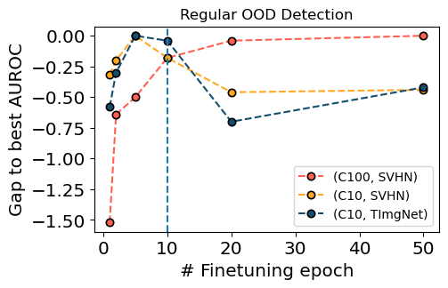
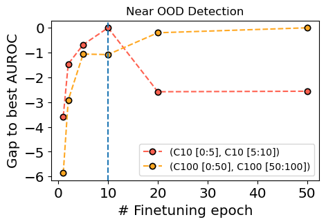
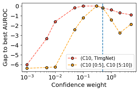
Figure 4: Further ablations on robustness of DCM to hyperparameters. Left: Relative AUROC of DCM on 3 regular OOD detection setting, where we vary the number of epochs in the second fine-tuning stage. Our default choice of 10 does not generally achieve the best performance. Middle: Similar to the plot on the left, but we experiment in the challenging near-OOD detection setting. Right: Relative AUROC of DCM where we vary the confidence weight $\lambda$.

Appendix H OOD Detection Ablations

H.1 Effect of confidence weight, $\lambda$

Figure 4 shows more results of the effect of $\lambda$ on our algorithm for OOD detection. We achieve the best performance when $\lambda=0.1\text{ or }0.3$ for (CIFAR-10, TinyImageNet) and (CIFAR-10 [0:5], CIFAR-10 [5:10]) respectively, as opposed to 0.5, our default choice.

H.2 Effect of number of epochs in the second fine-tuning stage

Since the second fine-tuning stage is the crucial step for our algorithm, we try different number of epochs for this stage and see its effect. Figure 4 shows the results. We see that the performance variation due to varying the number of epochs is negligible, implying DCM is robust to the choice of this hyper-parameters. We also see that in the 4/5 cases we have tried out, our default choice of 10 for the number of fine-tuning epochs do not achieve the best performance, justifying our experiment design.

H.3 More ablations on fraction of OOD examples in the uncertainty set

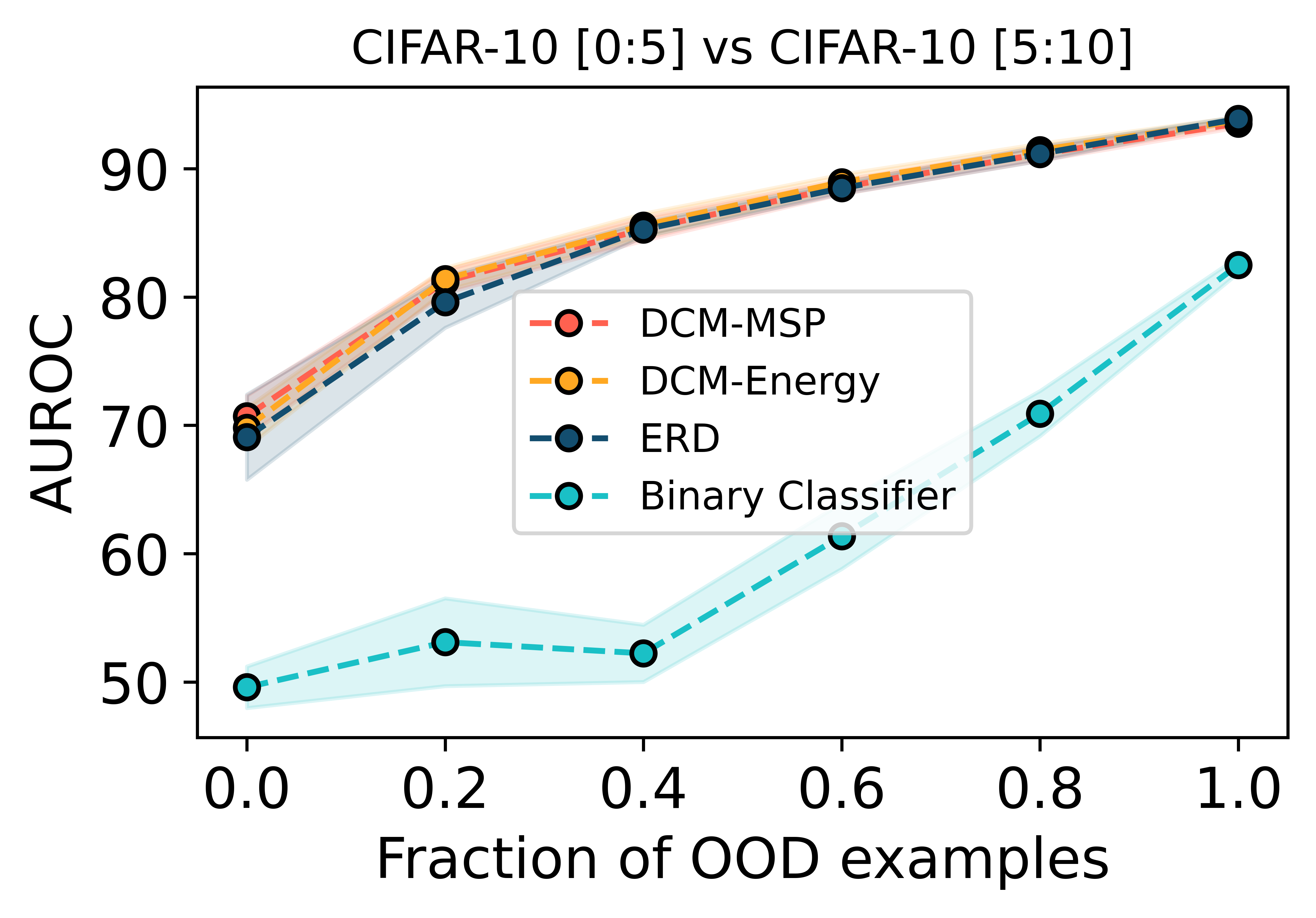
Figure 5: Performance of DCM on CIFAR-10 [0:5] vs CIFAR-10 [5:10] near-OOD detection task with various OOD proportions in the uncertainty dataset. The test dataset is fixed with 2500 ID and 500 OOD examples and is disjoint from the uncertainty dataset.

Similar to Figure 3, we vary the fraction of OOD examples in the uncertainty dataset and measure the performance of DCM for another near-OOD detection task, CIFAR-10 [0:5] vs CIFAR-10 [5:10]. Figure 5 shows our results. DCM outperform binary classifier for all OOD fractions, and performs similarly to ERD while using 1/3 the compute.

Appendix I Selective Classification Ablations

I.1 Effect of Weight of the Confidence Loss, $\lambda$

We investigate the sensitivity of DCM to the weight of the confidence loss, $\lambda$. In Figure 6, we plot the performance of DCM with various values of $\lambda$ on tasks constructed from the CIFAR-10 and CIFAR-10-C datasets. DCM performs best when $\lambda$ is large enough such that confidence is minimized on misclassified examples yet the impact on ID accuracy is negligible.

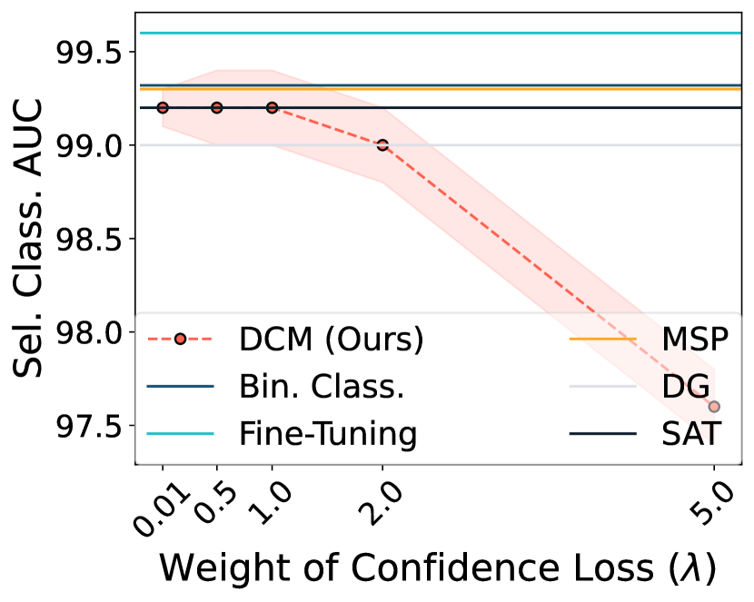
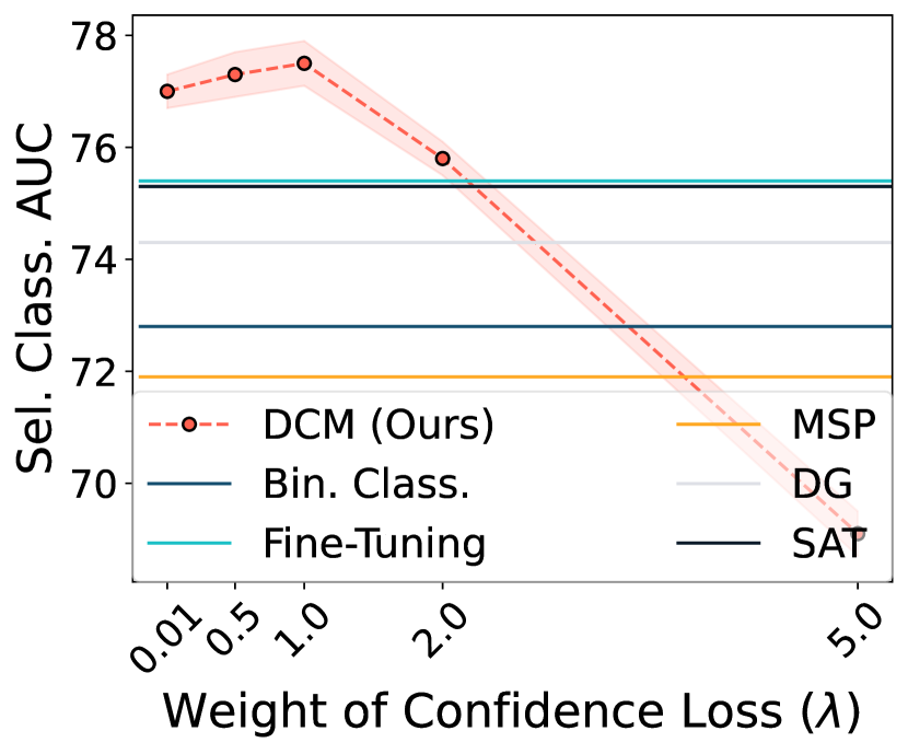
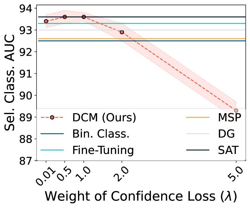
Figure 6: Selective classification performance of DCM when we vary the weight of the confidence loss term, $\lambda$. Left: CIFAR-10 $\rightarrow$ CIFAR-10, Middle: CIFAR-10 $\rightarrow$ CIFAR-10-C, Right: CIFAR-10 $\rightarrow$ CIFAR-10 + CIFAR-10-C. DCM consistently outperforms baselines under settings of distribution shift across a range of $\lambda$ values.

I.2 Effect of Validation Set Size

We investigate the sensitivity of DCM to the size of the validation set. In Figure 7, we plot the performance of DCM, Binary Classifier, Fine-Tuning, MSP, Deep Gamblers, and Self-Adaptive Training on the CIFAR-10 $\rightarrow$ CIFAR-10-C tasks with various validation set sizes. We find that DCM for selective classification is robust to a range of validation set sizes.

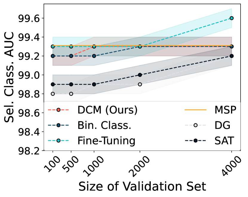
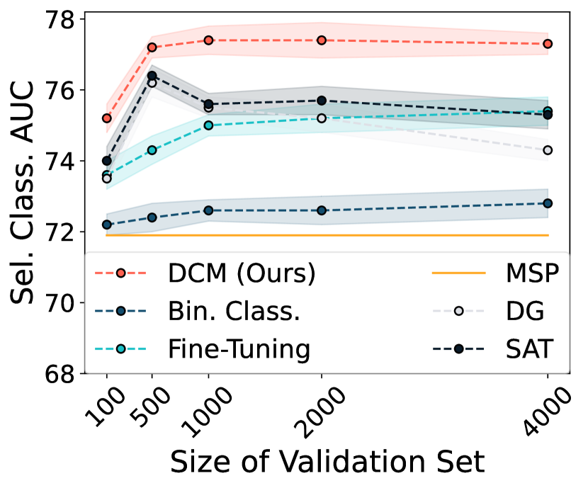
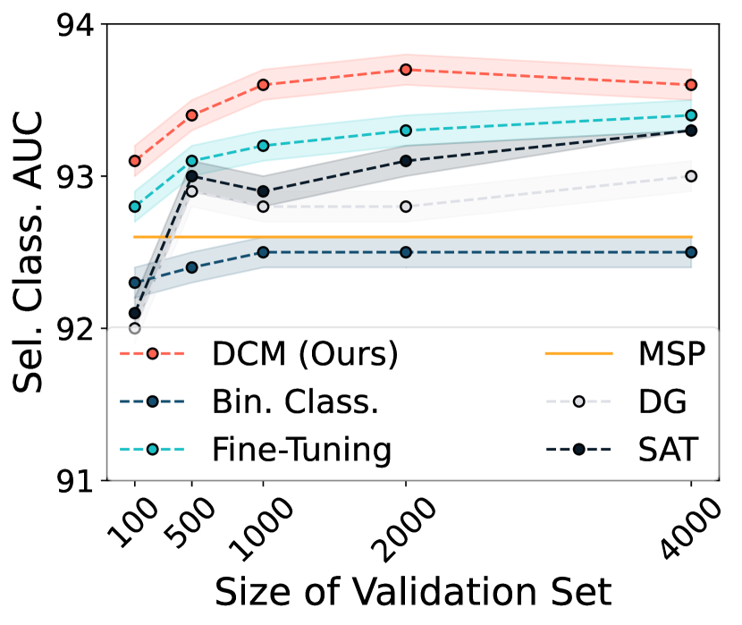
Figure 7: Selective classification performance of DCM when we vary the size of the validation set. Left: CIFAR-10 $\rightarrow$ CIFAR-10, Middle: CIFAR-10 $\rightarrow$ CIFAR-10-C, Right: CIFAR-10 $\rightarrow$ CIFAR-10 + CIFAR-10-C. DCM consistently outperforms baselines in distribution-shift settings with different validation set sizes.

Appendix J Selective Classification Experiment Details

J.1 Baselines

• MSP [21]: Also referred to as Softmax Response (SR), MSP directly uses the maximum softmax probability assigned by the model as an estimate of confidence. MSP has been shown to distinguish in-distribution test examples that the model gets correct from the ones that it gets incorrect.

• MaxLogit [23]: Directly uses the maximum logit outputted by the model as an estimate of confidence.

• Ensemble [31]: Uses an ensemble of 5 models, each trained with ERM on the ID train distribution with different random seeds. Following  Lakshminarayanan et al. [31], we use the entropy of the average softmax predictions of the models in the ensemble as the disagreement metric.

• Binary Classifier [25]: Trains a classifier on the labeled training and validation sets to predict inputs for which the base model will be correct versus incorrect. The classifier takes as input the softmax probabilities outputted by the base model. For the Binary Classifier, we found the MLP with softmax probabilities to work best compared to a random forest classifier and MLP with last-layer features.

• Fine-tuning: First trains a model on the training set, then fine-tunes the model on the validation set.

• Deep Gamblers [38]: Trains a classifier using a loss function derived from the doubling rate in a hypothetical horse race. Deep Gamblers introduces an extra $(c+1)$-th class that represents abstention. Minimizing this loss corresponds to maximizing the return, where the model makes a bet or prediction when confident, and abstains when uncertain.

• Self-Adaptive Training [24]: Trains a classifier using model predictions to dynamically calibrate the training process. SAT introduces an extra $(c+1)$-th class that represents abstention and uses training targets that are exponential moving averages of model predictions and ground-truth targets.

J.2 Datasets

• CIFAR-10 [28] $\rightarrow$ CIFAR-10-C [20]: The task is to classify images into 10 classes, where the target distribution contains severely corrupted images. We run experiments over 15 corruptions (brightness, contrast, defocus blur, elastic transform, fog, frost, gaussian noise, glass blur, impulse noise, jpeg compression, motion blur, pixelate, shot noise, snow, zoom blur) and use the data loading code from Croce et al. [8].

• Waterbirds [52, 44]: The Waterbirds dataset consists of images of landbirds and waterbirds on land or water backgrounds from the Places dataset [58]. The train set consists of 4,795 images, of which 3,498 are of waterbirds on water backgrounds, and 1,057 are of landbirds on land backgrounds. There are 184 images of waterbirds on land and 56 images of landbirds on water, which are the minority groups.

• Camelyon17 [27, 1]: The Camelyon17 dataset is a medical image classification task from the WILDS benchmark [27]. The dataset consists of $450,000$ whole-slide images of breast cancer metastases in lymph node from $5$ hospitals. The input is a $96\times 96$ image, and the label $y$ indicates whether there is a tumor in the image. The train set consists of lymph-node scans from 3 of the 5 hospitals, while the OOD validation set and OOD test datasets consists of lymph-node scans from the 4th and 5th hospitals, respectively.

• FMoW [27]: The FMoW dataset is a satellite image classification task from the WILDS benchmark [27]. The dataset consists of satellite images in various geographic locations from $2002-2018$. The input is a $224\times 224$ RGB satellite image, and the label $y$ is one of 62 building or land use categories. The train, validation, and test splits are based on the year that the images were taken: the train, ID validation, and ID test sets consist of images from $2002-2013$, the OOD validation set consists of images from $2013-2016$, and the OOD test set consists of images from $2016-2018$.

J.3 CIFAR-10 $\rightarrow$ CIFAR-10-C training details

• Architecture: We use a WideResNet-28-10 trained on the source CIFAR-10 distribution and attains 94.78% clean accuracy [8]. The base models for Deep Gamblers and Self-Adaptive Training use the same architecture with an additional 11th class in the final linear layer.

• Hyper-parameters: DCM, Fine-tuning, Binary Classifier, Deep Gamblers, and Self-Adaptive Training fine-tune the base models for 10 epochs. We perform hyperparameter tuning on a separate, held-out ID validation set. We tune all baselines over the learning rates $\{$1e-3, 1e-4, 1e-5$\}$, and use an initial learning rate of 1e-3 for all baselines except DCM, which uses an initial learning rate of 1e-4. For DCM, we use a confidence weight of $\lambda=0.5$ for all corruptions, as in  Hendrycks et al. [22]. For Deep Gamblers, we use a reward of $3.2$ and tune over rewards in the range $[2.0,4.2]$ with a step size of $0.2$, as in  Liu et al. [38]. We use SGD with a cosine learning rate schedule, weight decay of $5\times 10^{-4}$, and batch sizes of 128 and 256 for the fine-tuning set and uncertainty datasets, respectively.

• Validation and test set construction: We use the CIFAR-10 test set, and split it into a validation set of 5000 images, a test set of 4000 images, and set aside 1000 images for hyperparameter tuning. Similarly, for CIFAR-10-C, we use a validation set of 5000 images, and a test set of 4000 images.

  Each of our settings merges the train/val/test splits from the corresponding datasets. For example, Val = CIFAR-10, Test = CIFAR-10 + CIFAR-10-C uses a validation set of 5000 CIFAR-10 images for fine-tuning and a test set of 4000 CIFAR-10 and 4000 CIFAR-10-C images. Note that our combined CIFAR-10 + CIFAR-10-C test sets have a 1:1 clean-to-corrupted ratio.

• Augmentations: For DCM and fine-tuning, we use the same standard random horizontal flip and random crop ($32\times 32$).

J.4 Waterbirds training details

• Architecture: For our base model, we train a pretrained ResNet50 from torchvision on a subset of the Waterbirds train set (details of the split are described below). We follow the training details for the ERM baseline used by Sagawa et al. [44], and use SGD with a momentum term of 0.9, batch normalization, and no dropout. We use a fixed learning rate of 0.001, a $\ell_{2}$ penalty of $\lambda=0.0001$ and train for 300 epochs.

• Hyper-parameters: DCM, Fine-tuning, Binary Classifier, Deep Gamblers, and Self-Adaptive Training fine-tune the base models for 20 epochs. We perform hyperparameter tuning on a separate, held-out ID validation set. We tune all baselines over the learning rates $\{$1e-3, 1e-4, 1e-5$\}$, and use an initial learning rate of 1e-3 for all baselines except DCM, which uses an initial learning rate of 1e-4. For DCM, we use a confidence weight of $\lambda=0.5$. For Deep Gamblers, we use a reward of $1.4$ and tune over rewards in the range $[1.0,2.0]$ with a step size of $0.2$. We use SGD with a cosine learning rate schedule, weight decay of $5\times 10^{-4}$, and batch sizes of 64 and 128 for the fine-tuning set and uncertainty datasets, respectively.

• Validation and test set construction: We split the Waterbirds train set from Sagawa et al. [44] into two sets, one which we use to pretrain a base ERM model, and the other which we use as our ID validation set. We maintain group ratios, and the ID train and validation sets each contain 2,397 images, consisting of 1749 waterbirds on water, 528 landbirds on land, 92 waterbirds on land, and 28 landbirds on water. Our test set is the same test set from Sagawa et al. [44].

• Augmentations: DCM and Fine-Tuning use the train augmentations as in Sagawa et al. [44]: a random resized crop ($224\times 224$) and random horizontal flip.

J.5 Camelyon17 training details

• Architecture: We use a DenseNet121 pre-trained on the Camelyon17 train set from [27] as our base model. These models are trained for 5 epochs with a learning rate of $0.001$, $\ell_{2}$ regularization strength of $0.01$, batch size of 32, and SGD with momentum set to 0.9.

• Hyper-parameters: DCM, Fine-tuning, Binary Classifier, Deep Gamblers, and Self-Adaptive Training fine-tune the base models for 1 epoch. We perform hyperparameter tuning on a separate, held-out ID validation set. We tune all baselines over the learning rates $\{$1e-3, 1e-4, 1e-5$\}$, and use an initial learning rate of 1e-4 for all baselines. For DCM, we use a confidence weight of $\lambda=0.5$. For Deep Gamblers, we use a reward of $1.4$ and tune over rewards in the range $[1.0,2.0]$ with a step size of $0.2$. We use an AdamW optimizer with a cosine learning rate schedule, weight decay of $5\times 10^{-4}$, and batch size of 32 for the fine-tuning set and uncertainty datasets.

• Validation and test set construction: We use the train / ID val / OOD val / OOD test splits from the WILDS benchmark to construct our validation and test sets. For our ID validation set and ID test set, we split the Camelyon17 ID validation set into two equally-sized subsets and maintain group ratios. The Camelyon17 ID validation consists of samples from the same 3 hospitals as the train set. We use the OOD test set as our target distribution, which contains samples from the 5th hospital.

• Augmentations: DCM and Fine-tuning use random horizontal flips.

J.6 FMoW training details

• Architecture: We use FMoW ERM models from the WILDS benchmark [27] as our base model. These models use DenseNet121 pretrained on ImageNet with no $\ell_{2}$ regularization, Adam optimizer with an initial learning rate of 1e-4 that decays by $0.96$ per epoch, and train for 50 epochs with early stopping and batch size of 64.

• Hyper-parameters: DCM, Fine-tuning, Binary Classifier, Deep Gamblers, and Self-Adaptive Training fine-tune the base models for 5 epochs. We perform hyperparameter tuning on a separate, held-out ID validation set. We tune all baselines over the learning rates $\{$1e-3, 1e-4, 1e-5, 1e-6$\}$, and use an initial learning rate of 1e-3 for SAT, 1e-4 for Fine-tuning, Deep Gamblers, and Binary Classifier, and 1e-5 for DCM. For DCM, we use a confidence weight of $\lambda=0.1$ and tune over the weights $\{0.01,0.05,0.1,0.5,1.0,1.5\}$ on a held-out ID validation set. For Deep Gamblers, we use a reward of $35$ and tune over rewards in the range $[5.0,65.0]$ with a step size of $5.0$. We use an AdamW optimizer with a cosine learning rate schedule, weight decay of $5\times 10^{-4}$, and batch sizes of 16 and 32 for the uncertainty dataset and fine-tuning sets, respectively.

• Validation and test set construction: We use the train, ID validation, OOD validation, and OOD test splits from the WILDS benchmark as our validation and test sets. Specifically, we use the ID validation set, ID test set, and OOD test sets. For example, the task Val = FMoW ID, Test = FMoW ID + FMoW OOD uses the WILDS ID val set for validation, and the WILDS ID and OOD test sets for testing.

• Augmentations: DCM and Fine-tuning use random horizontal flips.

Appendix K Compute

All model training and experiments were conducted on a single NVIDIA RTX Titan or A40 GPU.

Method	ECE ($\downarrow$)	AUC ($\uparrow$)	Acc@90 ($\uparrow$)	Acc@95 ($\uparrow$)	Acc@99 ($\uparrow$)	Cov@90 ($\uparrow$)	Cov@95 ($\uparrow$)	Cov@99 ($\uparrow$)
Val = CIFAR-10, Test = CIFAR-10
MSP	0.5 (0.1)	99.3 (0.1)	98.4 (0.1)	97.2 (0.1)	95.7 (0.1)	100 (0.0)	100 (0.0)	87.0 (0.1)
MaxLogit	0.6 (0.1)	98.9 (0.1)	97.9 (0.1)	96.8 (0.1)	95.6 (0.1)	100 (0.0)	100 (0.0)	80.4 (0.1)
Ensemble	0.6 (0.1)	99.3 (0.1)	98.4 (0.1)	97.1 (0.1)	95.7 (0.1)	100 (0.0)	100 (0.0)	86.2 (0.1)
Binary Classifier	1.4 (0.1)	99.3 (0.1)	98.4 (0.1)	97.2 (0.2)	95.7 (0.2)	100 (0.0)	100 (0.0)	87.0 (2.3)
Fine-Tuning	0.3 (0.2)	99.6 (0.1)	99.1 (0.2)	98.7 (0.1)	97.5 (0.2)	100 (0.0)	100 (0.0)	91.6 (0.9)
DG	0.8 (0.1)	99.0 (0.0)	97.4 (0.1)	96.4 (0.0)	94.9 (0.1)	100 (0.0)	98.7 (0.1)	76.2 (1.7)
SAT	0.7 (0.1)	99.2 (0.0)	97.6 (0.1)	96.3 (0.0)	94.9 (0.1)	100 (0.0)	98.8 (0.1)	81.6 (1.1)
DCM (ours)	1.0 (0.2)	99.2 (0.2)	98.0 (0.2)	96.5 (0.2)	94.8 (0.2)	100 (0.0)	98.6 (0.4)	83.9 (1.0)
Val = CIFAR-10, Test = CIFAR-10 + CIFAR-10-C
MSP	9.3 (0.1)	92.6 (0.1)	80.4 (0.1)	78.3 (0.1)	76.4 (0.1)	72.4 (0.2)	60.6 (0.2)	27.4 (0.7)
MaxLogit	9.4 (0.0)	91.7 (0.0)	80.4 (0.0)	78.2 (0.0)	76.3 (0.0)	70.5 (0.1)	54.0 (0.3)	10.1 (0.3)
Ensemble	9.3 (0.1)	92.6 (0.1)	80.6 (0.1)	78.4 (0.1)	76.4 (0.1)	72.1 (0.3)	60.1 (0.3)	27.5 (0.8)
Binary Classifier	7.9 (0.1)	92.5 (0.1)	80.3 (0.1)	78.1 (0.1)	76.2 (0.1)	72.0 (0.2)	59.9 (0.3)	30.5 (1.7)
Fine-Tuning	8.2 (0.1)	93.4 (0.1)	81.3 (0.1)	78.9 (0.1)	77.0 (0.1)	74.2 (0.2)	63.4 (0.3)	42.4 (0.9)
DG	8.2 (0.0)	93.0 (0.1)	81.0 (0.0)	78.8 (0.0)	76.9 (0.0)	73.2 (0.2)	60.7 (0.5)	33.4 (1.2)
SAT	7.8 (0.0)	93.3 (0.0)	81.1 (0.0)	78.7 (0.1)	76.8 (0.0)	74.1 (0.0)	62.7 (0.1)	42.7 (0.3)
DCM (ours)	8.0 (0.1)	93.6 (0.1)	82.0 (0.1)	79.7 (0.1)	77.7 (0.1)	75.2 (0.1)	63.8 (0.3)	43.6 (0.9)
Val = CIFAR-10, Test = CIFAR-10-C
MSP	13.8 (0.1)	70.1 (0.1)	57.4 (0.2)	56.0 (0.2)	54.8 (0.1)	30.2 (0.3)	20.9 (0.5)	7.6 (0.3)
MaxLogit	14.6 (0.0)	71.7 (0.1)	59.4 (0.1)	58.0 (0.0)	56.8 (0.0)	23.2 (0.7)	11.3 (0.3)	3.5 (0.5)
Ensemble	14.5 (0.1)	72.9 (0.1)	59.8 (0.1)	58.2 (0.1)	57.0 (0.1)	27.6 (0.3)	16.6 (0.5)	5.0 (0.4)
Binary Classifier	13.6 (0.1)	72.8 (0.2)	59.5 (0.2)	58.0 (0.2)	56.7 (0.6)	28.5 (0.6)	16.4 (0.8)	8.2 (0.8)
Fine-Tuning	12.7 (0.1)	75.4 (0.1)	61.7 (0.2)	60.2 (0.3)	58.8 (0.3)	33.6 (0.8)	22.5 (0.8)	8.6 (0.5)
DG	12.7 (0.0)	74.3 (0.2)	61.4 (0.1)	59.9 (0.0)	58.7 (0.0)	28.4 (0.5)	17.2 (0.2)	7.2 (0.3)
SAT	12.5 (0.0)	75.3 (0.1)	61.4 (0.1)	59.8 (0.1)	58.4 (0.1)	32.5 (0.5)	22.0 (0.8)	8.6 (0.2)
DCM (ours)	12.3 (0.1)	77.5 (0.2)	64.1 (0.2)	62.4 (0.2)	61.0 (0.2)	37.6 (0.6)	25.2 (1.0)	8.9 (0.2)

Table 8: Selective classification performance on various distribution shift tasks constructed from the CIFAR-10 and CIFAR-10-C datasets. Bold numbers represent superior results, and parentheses show the standard error over 3 random seeds. DCM consistently outperforms MSP, MaxLogit, Deep Gamblers (DG), and Self-Adaptive Training (SAT), and outperforms all 7 prior methods when the validation and test sets are from different distributions.

Method	ECE ($\downarrow$)	AUC ($\uparrow$)	Acc@90 ($\uparrow$)	Acc@95 ($\uparrow$)	Acc@99 ($\uparrow$)	Cov@90 ($\uparrow$)	Cov@95 ($\uparrow$)	Cov@99 ($\uparrow$)
Val = Waterbirds-Train, Test = Waterbirds-Train
MSP	3.4 (0.0)	98.7 (0.0)	99.1 (0.0)	98.2 (0.0)	97.1 (0.0)	100 (0.0)	100 (0.0)	90.1 (0.0)
MaxLogit	3.2 (0.0)	98.6 (0.0)	99.3 (0.0)	98.2 (0.0)	97.2 (0.0)	100 (0.0)	100 (0.0)	91.0 (0.0)
Ensemble	3.1 (0.0)	98.7 (0.0)	98.9 (0.0)	98.2 (0.0)	97.2 (0.0)	100 (0.0)	100 (0.0)	88.8 (0.0)
Binary Classifier	3.4 (0.0)	98.7 (0.0)	99.1 (0.0)	98.2 (0.0)	97.1 (0.0)	100 (0.0)	100 (0.0)	90.1 (0.0)
Fine-Tuning	1.1 (0.0)	98.7 (0.0)	99.4 (0.0)	98.6 (0.0)	97.3 (0.0)	100 (0.0)	100 (0.0)	91.8 (0.0)
DG	1.3 (0.3)	98.5 (0.0)	98.8 (0.1)	98.0 (0.1)	97.3 (0.0)	100 (0.0)	100 (0.0)	86.9 (0.5)
SAT	0.7 (0.4)	98.6 (0.0)	99.1 (0.1)	98.3 (0.1)	97.4 (0.1)	100 (0.0)	100 (0.0)	91.3 (0.9)
DCM (ours)	1.8 (0.6)	98.7 (0.0)	99.2 (0.0)	98.3 (0.1)	97.2 (0.0)	100 (0.0)	100 (0.0)	91.9 (0.1)
Val = Waterbirds-Train, Test = Waterbirds-Test
MSP	15.1 (0.0)	94.4 (0.0)	88.2 (0.0)	86.8 (0.0)	85.3 (0.0)	83.9 (0.0)	60.9 (0.0)	27.5 (0.0)
MaxLogit	18.1 (0.0)	94.2 (0.0)	87.9 (0.0)	86.3 (0.0)	84.7 (0.0)	82.2 (0.0)	60.9 (0.0)	23.8 (0.0)
Ensemble	14.9 (0.0)	94.4 (0.0)	88.4 (0.0)	87.0 (0.0)	85.4 (0.0)	85.0 (0.0)	62.0 (0.0)	25.6 (0.0)
Binary Classifier	16.4 (0.3)	94.0 (0.2)	87.5 (0.3)	86.1 (0.2)	84.8 (0.2)	81.2 (1.8)	59.8 (2.0)	24.2 (1.1)
Fine-Tuning	15.3 (0.4)	94.7 (0.2)	89.0 (0.5)	87.2 (0.5)	86.2 (0.5)	86.8 (1.4)	64.0 (2.7)	27.9 (2.7)
DG	17.3 (0.4)	94.8 (0.1)	88.6 (0.2)	87.0 (0.2)	85.8 (0.2)	85.4 (0.6)	67.3 (1.1)	29.4 (0.4)
SAT	17.5 (0.2)	95.1 (0.0)	88.9 (0.1)	87.0 (0.1)	85.6 (0.1)	87.2 (0.4)	70.0 (0.3)	34.4 (0.4)
DCM (ours)	13.9 (0.7)	95.0 (0.1)	89.5 (0.3)	88.0 (0.4)	86.6 (0.4)	88.2 (0.8)	66.5 (0.3)	29.8 (1.1)

Table 9: Selective classification on the Waterbirds spurious correlation dataset. Bold numbers represent superior results, and parentheses show the standard error over 3 random seeds. DCM consistently outperforms all 7 prior methods when the validation and test sets are from different distributions, suggesting that DCM is effective in spurious correlation settings.

Method	ECE ($\downarrow$)	AUC ($\uparrow$)	Acc@90 ($\uparrow$)	Acc@95 ($\uparrow$)	Acc@99 ($\uparrow$)	Cov@90 ($\uparrow$)	Cov@95 ($\uparrow$)	Cov@99 ($\uparrow$)
Val = Camelyon17 ID Val-1, Test = Camelyon17 ID Val-2
MSP	16.3 (10.4)	96.9 (2.2)	92.0 (5.9)	90.8 (6.4)	89.5 (6.6)	87.2 (10.5)	78.6 (17.5)	60.5 (25.5)
MaxLogit	16.4 (10.2)	97.0 (2.2)	92.2 (5.8)	91.0 (6.4)	89.8 (6.5)	87.8 (10.0)	79.1 (17.1)	60.1 (27.0)
Ensemble	15.7 (11.2)	99.1 (2.7)	96.8 (5.9)	95.9 (6.7)	95.1 (6.8)	100.0 (10.5)	99.4 (18.1)	73.2 (27.7)
Binary Classifier	16.3 (9.2)	97.0 (4.5)	92.3 (5.9)	91.4 (6.0)	90.3 (6.7)	88.1 (10.2)	79.3 (16.8)	61.0 (24.2)
Fine-Tuning	2.8 (0.2)	99.8 (0.0)	99.7 (0.0)	99.4 (0.1)	98.6 (0.2)	100.0 (0.0)	100.0 (0.0)	97.3 (0.7)
DG	3.4 (2.1)	99.8 (0.0)	99.6 (0.1)	99.2 (0.3)	98.2 (0.4)	100.0 (0.0)	100.0 (0.0)	96.1 (1.7)
SAT	1.6 (0.0)	99.8 (0.0)	99.7 (0.0)	99.4 (0.0)	98.5 (0.0)	100.0 (0.0)	100.0 (0.0)	96.7 (0.3)
DCM (ours)	9.9 (0.3)	99.5 (0.1)	98.6 (0.2)	98.0 (0.0)	96.6 (0.2)	100.0 (0.0)	100.0 (0.0)	82.4 (5.3)
Val = Camelyon17 ID Val-1, Test = Camelyon17 ID Val-2 + Camelyon17 OOD Test
MSP	25.9 (6.4)	85.8 (3.7)	74.1 (5.1)	73.1 (4.9)	72.2 (4.8)	40.6 (7.8)	29.4 (8.1)	7.4 (3.3)
MaxLogit	25.9 (6.4)	85.8 (3.7)	74.2 (5.1)	73.1 (5.0)	72.2 (4.8)	40.7 (7.9)	29.4 (8.2)	7.7 (3.6)
Ensemble	19.6 (6.7)	86.5 (4.1)	78.1 (4.8)	76.8 (5.2)	75.8 (4.2)	25.8 (8.1)	18.7 (8.4)	11.5 (3.5)
Binary Classifier	26.3 (6.0)	86.2 (3.3)	74.4 (5.0)	73.4 (4.9)	72.7 (4.4)	41.0 (8.1)	29.8 (8.2)	7.5 (3.5)
Fine-Tuning	20.5 (1.9)	88.9 (2.2)	79.8 (3.5)	78.6 (3.4)	77.6 (3.3)	44.2 (5.8)	33.1 (2.8)	9.7 (6.3)
DG	27.5 (7.3)	88.1 (4.1)	77.2 (6.5)	75.8 (6.3)	74.8 (6.0)	51.3 (14.3)	36.4 (9.3)	6.2 (3.8)
SAT	24.3 (2.1)	86.3 (0.4)	74.8 (1.1)	73.8 (1.1)	73.0 (1.2)	35.2 (1.3)	28.3 (1.6)	15.2 (1.4)
DCM (ours)	8.9 (1.5)	93.5 (0.6)	85.5 (1.0)	83.8 (1.0)	82.5 (0.9)	74.1 (4.3)	50.3 (6.5)	16.4 (0.6)
Val = Camelyon17 ID Val-1, Test = Camelyon17 OOD Test
MSP	28.2 (5.4)	82.2 (3.9)	70.4 (4.8)	69.5 (4.6)	68.8 (4.4)	31.5 (6.8)	21.8 (7.8)	2.4 (0.4)
MaxLogit	28.2 (5.4)	82.1 (3.9)	70.4 (4.8)	69.5 (4.6)	68.8 (4.4)	31.4 (6.9)	21.9 (7.8)	2.4 (0.4)
Ensemble	21.1 (5.6)	81.4 (4.4)	74.0 (5.2)	72.8 (4.3)	72.0 (4.7)	13.4 (7.3)	9.8 (8.1)	4.6 (0.3)
Binary Classifier	28.0 (5.3)	82.4 (3.9)	70.5 (4.4)	70.1 (4.2)	69.5 (6.5)	32.1 (5.6)	22.1 (7.3)	2.5 (0.4)
Fine-Tuning	23.6 (2.0)	84.2 (3.8)	75.4 (4.2)	74.3 (4.1)	73.5 (4.0)	31.4 (6.0)	21.6 (6.5)	3.8 (3.1)
DG	31.6 (8.5)	84.8 (5.2)	72.1 (7.9)	70.9 (7.7)	70.1 (7.3)	43.3 (11.2)	31.9 (8.0)	5.8 (4.0)
SAT	21.7 (2.3)	80.3 (0.6)	71.9 (0.8)	71.3 (1.0)	70.8 (1.0)	20.3 (3.6)	5.9 (4.0 )	0.0 (0.0)
DCM (ours)	11.5 (2.1)	91.6 (1.1)	82.5 (1.2)	80.9 (1.1)	79.7 (1.1)	62.5 (8.2)	40.3 (7.5)	9.7 (2.9)
Val = FMoW ID Val, Test = FMoW ID Test
MSP	1.8 (0.4)	81.3 (0.4)	62.6 (0.1)	60.9 (0.1)	58.7 (0.1)	36.7 (1.3)	18.4 (5.8)	3.7 (1.8)
MaxLogit	1.8 (0.4)	80.1 (0.2)	62.7 (0.2)	60.6 (0.1)	58.8 (0.1)	29.7 (0.8)	10.7 (2.2)	0.8 (0.4)
Ensemble	0.8 (0.0)	85.5 (0.0)	68.4 (0.1)	66.1 (0.1)	64.2 (0.1)	44.8 (0.3)	31.5 (0.1)	10.6 (0.8)
Binary Classifier	1.9 (0.4)	82.3 (0.3)	64.3 (0.1)	62.0 (0.2)	60.2 (0.1)	37.6 (0.5)	20.9 (4.3)	3.7 (2.7)
Fine-Tuning	1.2 (0.5)	82.8 (0.9)	64.0 (1.2)	61.7 (1.3)	59.9 (1.2)	39.5 (2.4)	27.0 (2.8)	5.9 (1.2)
DG	1.8 (0.1)	75.8 (0.2)	62.4 (0.9)	60.9 (0.5)	59.9 (0.4)	12.9 (0.6)	2.6 (1.8)	0.1 (0.0)
SAT	1.1 (0.0)	81.1 (0.3)	63.0 (0.5)	60.8 (0.5)	59.1 (0.5)	33.5 (0.5)	18.8 (1.0)	4.3 (0.9)
DCM (ours)	1.1 (0.5)	82.9 (1.1)	64.2 (1.2)	61.7 (1.3)	59.9 (1.1)	39.4 (2.5)	26.7 (3.5)	6.3 (2.0)
Val = FMoW ID Val, Test = FMoW ID Test + FMoW OOD Test
MSP	2.3 (0.4)	77.1 (0.5)	57.9 (0.1)	55.9 (0.2)	54.2 (0.0)	25.4 (2.3)	11.0 (4.6)	1.2 (0.6)
MaxLogit	2.3 (0.5)	75.8 (0.1)	57.8 (0.1)	55.7 (0.1)	54.2 (0.0)	19.4 (0.3)	4.3 (0.9)	0.3 (0.2)
Ensemble	1.3 (0.0)	81.7 (0.0)	63.2 (0.0)	61.2 (0.0)	59.4 (0.0)	35.6 (0.2)	24.3 (0.1)	5.6 (0.2)
Binary Classifier	2.5 (0.4)	78.0 (0.4)	59.3 (0.0)	57.3 (0.0)	55.6 (0.0)	27.5 (1.5)	9.3 (6.2)	1.2 (0.9)
Fine-Tuning	1.7 (0.3)	78.6 (0.8)	58.6 (1.2)	56.5 (1.1)	54.8 (1.1)	30.8 (2.1)	19.1 (1.7)	3.0 (0.3)
DG	2.2 (0.0)	71.6 (0.2)	57.5 (0.3)	56.1 (0.2)	55.1 (0.2)	5.0 (0.2)	0.2 (0.1)	0.0 (0.0)
SAT	1.4 (0.0)	76.7 (0.2)	57.8 (0.4)	55.8 (0.4)	54.3 (0.4)	24.8 (0.3)	11.2 (0.8)	0.5 (0.2)
DCM (ours)	1.5 (0.3)	78.9 (1.1)	58.8 (1.3)	56.7 (1.3)	55.0 (1.3)	30.7 (2.0)	20.1 (2.2)	3.8 (1.1)
Val = FMoW ID Val, Test = FMoW OOD Test
MSP	2.6 (0.5)	74.5 (0.6)	55.2 (0.2)	53.4 (0.3)	52.0 (0.1)	20.6 (3.2)	8.4 (3.5)	1.3 (0.4)
MaxLogit	2.6 (0.5)	73.3 (0.2)	55.2 (0.0)	53.3 (0.1)	51.9 (0.1)	13.7 (0.4)	3.2 (0.8)	0.3 (0.1)
Ensemble	1.6 (0.0)	79.5 (0.0)	60.7 (0.1)	58.6 (0.1)	57.0 (0.1)	31.1 (0.1)	20.8 (0.4)	3.3 (0.6)
Binary Classifier	2.8 (0.5)	75.6 (0.5)	56.8 (0.1)	54.9 (0.0)	53.3 (0.0)	21.1 (3.8)	7.6 (4.8)	1.0 (0.4)
Fine-Tuning	2.0 (0.3)	76.2 (0.8)	56.0 (0.9)	53.9 (0.9)	52.4 (1.0)	26.8 (1.4)	14.8 (1.3)	1.7 (0.1)
DG	2.5 (0.0)	69.2 (0.3)	54.9 (0.2)	53.7 (0.1)	52.6 (0.0)	2.7 (0.8)	0.1 (0.1)	0.0 (0.0)
SAT	1.6 (0.0)	74.1 (0.2)	55.1 (0.4)	53.2 (0.3)	51.8 (0.3)	20.1 (0.4)	7.1 (1.1)	0.3 (0.1)
DCM (ours)	1.8 (0.3)	76.4 (1.1)	56.2 (1.4)	54.1 (1.3)	52.4 (1.2)	26.8 (1.6)	16.3 (1.7)	2.4 (0.5)

Table 10: Selective classification on the Camelyon17 and FMoW domain shift datasets. Bold numbers represent best performance, and parentheses show the standard error over 3 random seeds. On Camelyon17, DCM consistently outperforms all 7 prior methods when the validation and test sets are from different distributions. On FMoW, DCM has the second-highest AUC after Ensemble, while using only $1/5$ of the compute.

References

- Bandi et al. [2018] Bandi, P., Geessink, O., Manson, Q., Van Dijk, M., Balkenhol, M., Hermsen, M., Bejnordi, B. E., Lee, B., Paeng, K., Zhong, A., et al. From detection of individual metastases to classification of lymph node status at the patient level: the camelyon17 challenge. IEEE transactions on medical imaging, 38(2):550–560, 2018.
- Bendale & Boult [2016] Bendale, A. and Boult, T. E. Towards open set deep networks. In Proceedings of the IEEE conference on computer vision and pattern recognition, pp. 1563–1572, 2016.
- Canonne [2022] Canonne, C. L. A short note on an inequality between kl and tv, 2022.
- Chan et al. [2020] Chan, A., Alaa, A., Qian, Z., and Van Der Schaar, M. Unlabelled data improves Bayesian uncertainty calibration under covariate shift. In III, H. D. and Singh, A. (eds.), Proceedings of the 37th International Conference on Machine Learning, volume 119 of Proceedings of Machine Learning Research, pp. 1392–1402. PMLR, 13–18 Jul 2020.
- Chen et al. [2021] Chen, J., Li, Y., Wu, X., Liang, Y., and Jha, S. Atom: Robustifying out-of-distribution detection using outlier mining. In Machine Learning and Knowledge Discovery in Databases. Research Track: European Conference, ECML PKDD 2021, Bilbao, Spain, September 13–17, 2021, Proceedings, Part III 21, pp. 430–445. Springer, 2021.
- Corbière et al. [2019] Corbière, C., Thome, N., Bar-Hen, A., Cord, M., and Pérez, P. Addressing failure prediction by learning model confidence. Advances in Neural Information Processing Systems, 32, 2019.
- Cortes et al. [2016] Cortes, C., DeSalvo, G., and Mohri, M. Boosting with abstention. Advances in Neural Information Processing Systems, 29, 2016.
- Croce et al. [2020] Croce, F., Andriushchenko, M., Sehwag, V., Debenedetti, E., Flammarion, N., Chiang, M., Mittal, P., and Hein, M. Robustbench: a standardized adversarial robustness benchmark. arXiv preprint arXiv:2010.09670, 2020.
- Deng et al. [2009] Deng, J., Socher, R., Fei-Fei, L., Dong, W., Li, K., and Li, L.-J. Imagenet: A large-scale hierarchical image database. In 2009 IEEE Conference on Computer Vision and Pattern Recognition (CVPR), volume 00, pp. 248–255, 06 2009. doi: 10.1109/CVPR.2009.5206848.
- DeVries & Taylor [2018] DeVries, T. and Taylor, G. W. Learning confidence for out-of-distribution detection in neural networks. arXiv preprint arXiv:1802.04865, 2018.
- Du et al. [2022] Du, X., Wang, Z., Cai, M., and Li, Y. Vos: Learning what you don’t know by virtual outlier synthesis. arXiv preprint arXiv:2202.01197, 2022.
- Feng et al. [2019] Feng, J., Sondhi, A., Perry, J., and Simon, N. Selective prediction-set models with coverage guarantees. arXiv preprint arXiv:1906.05473, 2019.
- Fisch et al. [2022] Fisch, A., Jaakkola, T., and Barzilay, R. Calibrated selective classification. arXiv preprint arXiv:2208.12084, 2022.
- Fumera & Roli [2002] Fumera, G. and Roli, F. Support vector machines with embedded reject option. In Pattern Recognition with Support Vector Machines: First International Workshop, SVM 2002 Niagara Falls, Canada, August 10, 2002 Proceedings, pp. 68–82. Springer, 2002.
- Gangrade et al. [2021] Gangrade, A., Kag, A., and Saligrama, V. Selective classification via one-sided prediction. In International Conference on Artificial Intelligence and Statistics, pp. 2179–2187. PMLR, 2021.
- Geifman & El-Yaniv [2017] Geifman, Y. and El-Yaniv, R. Selective classification for deep neural networks. Advances in neural information processing systems, 30, 2017.
- Guo et al. [2017] Guo, C., Pleiss, G., Sun, Y., and Weinberger, K. Q. On calibration of modern neural networks. In International conference on machine learning, pp. 1321–1330. PMLR, 2017.
- He et al. [2015] He, K., Zhang, X., Ren, S., and Sun, J. Deep residual learning for image recognition, 2015.
- Hellman [1970] Hellman, M. E. The nearest neighbor classification rule with a reject option. IEEE Transactions on Systems Science and Cybernetics, 6(3):179–185, 1970. doi: 10.1109/TSSC.1970.300339.
- Hendrycks & Dietterich [2019] Hendrycks, D. and Dietterich, T. Benchmarking neural network robustness to common corruptions and perturbations. arXiv preprint arXiv:1903.12261, 2019.
- Hendrycks & Gimpel [2016] Hendrycks, D. and Gimpel, K. A baseline for detecting misclassified and out-of-distribution examples in neural networks. arXiv preprint arXiv:1610.02136, 2016.
- Hendrycks et al. [2018] Hendrycks, D., Mazeika, M., and Dietterich, T. Deep anomaly detection with outlier exposure. arXiv preprint arXiv:1812.04606, 2018.
- Hendrycks et al. [2022] Hendrycks, D., Basart, S., Mazeika, M., Zou, A., Kwon, J., Mostajabi, M., Steinhardt, J., and Song, D. Scaling out-of-distribution detection for real-world settings. In Chaudhuri, K., Jegelka, S., Song, L., Szepesvari, C., Niu, G., and Sabato, S. (eds.), Proceedings of the 39th International Conference on Machine Learning, volume 162 of Proceedings of Machine Learning Research, pp. 8759–8773. PMLR, 17–23 Jul 2022.
- Huang et al. [2020] Huang, L., Zhang, C., and Zhang, H. Self-adaptive training: beyond empirical risk minimization. Advances in neural information processing systems, 33:19365–19376, 2020.
- Kamath et al. [2020] Kamath, A., Jia, R., and Liang, P. Selective question answering under domain shift. arXiv preprint arXiv:2006.09462, 2020.
- Katz-Samuels et al. [2022] Katz-Samuels, J., Nakhleh, J. B., Nowak, R., and Li, Y. Training OOD detectors in their natural habitats. In Chaudhuri, K., Jegelka, S., Song, L., Szepesvari, C., Niu, G., and Sabato, S. (eds.), Proceedings of the 39th International Conference on Machine Learning, volume 162 of Proceedings of Machine Learning Research, pp. 10848–10865. PMLR, 17–23 Jul 2022.
- Koh et al. [2021] Koh, P. W., Sagawa, S., Marklund, H., Xie, S. M., Zhang, M., Balsubramani, A., Hu, W., Yasunaga, M., Phillips, R. L., Gao, I., et al. Wilds: A benchmark of in-the-wild distribution shifts. In International Conference on Machine Learning, pp. 5637–5664. PMLR, 2021.
- Krizhevsky et al. [a] Krizhevsky, A., Nair, V., and Hinton, G. Cifar-10 (canadian institute for advanced research). a.
- Krizhevsky et al. [b] Krizhevsky, A., Nair, V., and Hinton, G. Cifar-100 (canadian institute for advanced research). b.
- Kumar et al. [2020] Kumar, A., Zhou, A., Tucker, G., and Levine, S. Conservative q-learning for offline reinforcement learning. Advances in Neural Information Processing Systems, 33:1179–1191, 2020.
- Lakshminarayanan et al. [2017] Lakshminarayanan, B., Pritzel, A., and Blundell, C. Simple and scalable predictive uncertainty estimation using deep ensembles. Advances in neural information processing systems, 30, 2017.
- Le & Yang [2015] Le, Y. and Yang, X. S. Tiny imagenet visual recognition challenge. 2015.
- Lee et al. [2017] Lee, K., Lee, H., Lee, K., and Shin, J. Training confidence-calibrated classifiers for detecting out-of-distribution samples. arXiv preprint arXiv:1711.09325, 2017.
- Lee et al. [2018] Lee, K., Lee, K., Lee, H., and Shin, J. A simple unified framework for detecting out-of-distribution samples and adversarial attacks, 2018.
- Liang et al. [2017a] Liang, S., Li, Y., and Srikant, R. Enhancing the reliability of out-of-distribution image detection in neural networks. arXiv preprint arXiv:1706.02690, 2017a.
- Liang et al. [2017b] Liang, S., Li, Y., and Srikant, R. Principled detection of out-of-distribution examples in neural networks. CoRR, abs/1706.02690, 2017b.
- Liu et al. [2020] Liu, W., Wang, X., Owens, J., and Li, Y. Energy-based out-of-distribution detection. Advances in Neural Information Processing Systems, 33:21464–21475, 2020.
- Liu et al. [2019] Liu, Z., Wang, Z., Liang, P. P., Salakhutdinov, R. R., Morency, L.-P., and Ueda, M. Deep gamblers: Learning to abstain with portfolio theory. Advances in Neural Information Processing Systems, 32, 2019.
- Mohseni et al. [2020] Mohseni, S., Pitale, M., Yadawa, J., and Wang, Z. Self-supervised learning for generalizable out-of-distribution detection. In Proceedings of the AAAI Conference on Artificial Intelligence, volume 34, pp. 5216–5223, 2020.
- Netzer et al. [2011] Netzer, Y., Wang, T., Coates, A., Bissacco, A., Wu, B., and Ng, A. Y. Reading digits in natural images with unsupervised feature learning. In NIPS Workshop on Deep Learning and Unsupervised Feature Learning 2011, 2011.
- Nixon et al. [2019] Nixon, J., Dusenberry, M. W., Zhang, L., Jerfel, G., and Tran, D. Measuring calibration in deep learning. In CVPR workshops, volume 2, 2019.
- Pinsker [1964] Pinsker, M. S. Information and information stability of random variables and processes. Holden-Day, 1964.
- Ren et al. [2021] Ren, J., Fort, S., Liu, J. Z., Roy, A. G., Padhy, S., and Lakshminarayanan, B. A simple fix to mahalanobis distance for improving near-ood detection. CoRR, abs/2106.09022, 2021.
- Sagawa et al. [2019] Sagawa, S., Koh, P. W., Hashimoto, T. B., and Liang, P. Distributionally robust neural networks for group shifts: On the importance of regularization for worst-case generalization. arXiv preprint arXiv:1911.08731, 2019.
- Setlur et al. [2022] Setlur, A., Eysenbach, B., Smith, V., and Levine, S. Adversarial unlearning: Reducing confidence along adversarial directions. arXiv preprint arXiv:2206.01367, 2022.
- Simonyan & Zisserman [2014] Simonyan, K. and Zisserman, A. Very deep convolutional networks for large-scale image recognition. arXiv preprint arXiv:1409.1556, 2014.
- Sun et al. [2022] Sun, Y., Ming, Y., Zhu, X., and Li, Y. Out-of-distribution detection with deep nearest neighbors. In International Conference on Machine Learning, pp. 20827–20840. PMLR, 2022.
- Tajwar et al. [2021] Tajwar, F., Kumar, A., Xie, S. M., and Liang, P. No true state-of-the-art? ood detection methods are inconsistent across datasets. arXiv preprint arXiv:2109.05554, 2021.
- Ţifrea et al. [2020] Ţifrea, A., Stavarache, E., and Yang, F. Novelty detection using ensembles with regularized disagreement. arXiv preprint arXiv:2012.05825, 2020.
- Tifrea et al. [2022] Tifrea, A., Stavarache, E., and Yang, F. Semi-supervised novelty detection using ensembles with regularized disagreement. In Uncertainty in Artificial Intelligence, pp. 1939–1948. PMLR, 2022.
- Torralba et al. [2008] Torralba, A., Fergus, R., and Freeman, W. T. 80 million tiny images: A large data set for nonparametric object and scene recognition. IEEE Transactions on Pattern Analysis and Machine Intelligence, 30(11):1958–1970, 2008. doi: 10.1109/TPAMI.2008.128.
- Wah et al. [2011] Wah, C., Branson, S., Welinder, P., Perona, P., and Belongie, S. The caltech-ucsd birds-200-2011 dataset. 2011.
- Wei et al. [2022] Wei, H., Xie, R., Cheng, H., Feng, L., An, B., and Li, Y. Mitigating neural network overconfidence with logit normalization. In International Conference on Machine Learning, pp. 23631–23644. PMLR, 2022.
- Xu et al. [2015] Xu, P., Ehinger, K. A., Zhang, Y., Finkelstein, A., Kulkarni, S. R., and Xiao, J. Turkergaze: Crowdsourcing saliency with webcam based eye tracking, 2015.
- Yu et al. [2015] Yu, F., Zhang, Y., Song, S., Seff, A., and Xiao, J. Lsun: Construction of a large-scale image dataset using deep learning with humans in the loop. arXiv preprint arXiv:1506.03365, 2015.
- Zagoruyko & Komodakis [2016] Zagoruyko, S. and Komodakis, N. Wide residual networks, 2016.
- Zhang et al. [2017] Zhang, C., Bengio, S., Hardt, M., Recht, B., and Vinyals, O. Understanding deep learning requires rethinking generalization. 5th International Conference on Learning Representations (ICLR), 2017.
- Zhou et al. [2017] Zhou, B., Lapedriza, A., Khosla, A., Oliva, A., and Torralba, A. Places: A 10 million image database for scene recognition. IEEE transactions on pattern analysis and machine intelligence, 40(6):1452–1464, 2017.