Traveling kink oscillations of coronal loops launched by a solar flare

Abstract

Context. Kink oscillations, which are often associated with magnetohydrodynamic waves, are usually identified as transverse displacement oscillations of loop-like structures. However, the traveling kink oscillation evolving to a standing wave has rarely been reported.

Aims. We investigate the traveling kink oscillation triggered by a solar flare on 2022 September 29. The traveling kink wave is then evolved to a standing kink oscillation of the coronal loop.

Methods. The observational data mainly come from the Solar Upper Transition Region Imager (SUTRI), Atmospheric Imaging Assembly (AIA), and Spectrometer/Telescope for Imaging X-rays (STIX). In order to accurately identify the diffuse coronal loops, we applied a multi-Gaussian normalization (MGN) image processing technique to the extreme ultraviolet (EUV) image sequences at SUTRI 465 Å, AIA 171 Å, and 193 Å. A sine function within the decaying term and linear trend is used to extract the oscillation periods and amplitudes. With the aid of a differential emission measure analysis, the coronal seismology is applied to diagnose key parameters of the oscillating loop. At last, the wavelet transform is used to seek for multiple harmonics of the kink wave.

Results. The transverse oscillations with an apparent decay in amplitude and nearly perpendicular to the oscillating loop are observed in the passbands of SUTRI 465 Å, AIA 171 Å, and 193 Å. The decaying oscillation is launched by a solar flare erupted close to one footpoint of coronal loops and then it propagates along several loops. Next, the traveling kink wave is evolved to a standing kink oscillation. The standing kink oscillation along one coronal loop has a similar period of $\sim$6.3 minutes at multiple wavelengths, and the decaying time is estimated at $\sim$9.6$-$10.6 minutes. Finally, two dominant periods of 5.1 minutes and 2.0 minutes are detected in another oscillating loop, suggesting the coexistence of the fundamental and third harmonics.

Conclusions. First, we report the evolution of a traveling kink pulse to a standing kink wave along coronal loops that has been induced by a solar flare. We also detected a third-harmonic kink wave in an oscillating loop.

1 Introduction

The solar corona, which lies in the upper atmosphere of the Sun, is filled with various hot and magnetic structures, such as coronal loops. These loop systems often reveal transverse oscillations, and they are commonly connected to magnetohydrodynamic (MHD) waves in the solar corona (see Nakariakov & Kolotkov, 2020, for a recent review). The kink-mode oscillation, which is always perpendicular to the oscillating loop and non-axisymmetric, is one of the most studied MHD waves in the solar corona (Nakariakov et al., 2021; Li et al., 2023a). It was first identified as the transverse displacement oscillation of coronal loops in extreme ultraviolet (EUV) image sequences. Those observed kink-mode oscillations were characterized by large-scale amplitudes ($\gg$1 Mm) and quickly decaying within a few wave periods, termed as ”decaying oscillations” (Nakariakov et al., 1999; Aschwanden et al., 2002; Goddard et al., 2016; Li et al., 2017). Later on, the kink-mode oscillation without significant decaying was observed as the transverse displacement in EUV images (Wang et al., 2012) or the Doppler shift oscillation in coronal spectral lines (Tian et al., 2012). Such decayless oscillations often show small-scale amplitudes ($<$1 Mm) and can last for several wave periods or even many more (Anfinogentov et al., 2015; Karampelas & Van Doorsselaere, 2021; Mandal et al., 2022). Over the various observations, kink-mode oscillations could be seen in nearly all the loop-like structures, such as coronal loops, hot flare loops, prominence threads, and even coronal bright points, since these structures are all magnetic in nature; for instance, they all could be regarded as thin magnetic flux tubes (e.g., Nakariakov et al., 1999; Goossens et al., 2013; Goddard et al., 2016; Li et al., 2018a, 2022a, 2023b; Nakariakov et al., 2022; Zhang et al., 2022). More interestingly, kink oscillations of a plasma slab could be seen in microwave emissions (Li et al., 2020), which could be used to explain the quasi-periodic pulsation at the wavelength of microwave that is observed in the solar or stellar flare (e.g., Kaltman & Kupriyanova, 2023).

The kink-mode oscillation, in particular for the decaying oscillation, is presumed to be excited by an impulsive solar eruption, that is, a solar flare, a coronal jet, a flux rope, and so on (e.g., Zimovets & Nakariakov, 2015; Shen et al., 2017, 2018; Reeves et al., 2020; Zhang, 2020). The observed oscillation periods range from several minutes to a few tens of minutes in duration, while the decaying time is roughly equal to several oscillation periods (Goddard et al., 2016; Nechaeva et al., 2019; Ning et al., 2022). Conversely, decayless kink oscillations have been demonstrated to be omnipresent in the solar corona, but they appear to have no obvious connection to any solar eruptive events (e.g., Tian et al., 2012; Anfinogentov et al., 2015; Nakariakov et al., 2016; Guo et al., 2022). Their displacement amplitudes are smaller than the minor radius of oscillating loops, and their oscillation periods could range from a few tens seconds to several hundreds seconds (Pascoe et al., 2016; Li et al., 2018b; Mandal et al., 2021; Shi et al., 2022; Zhong et al., 2022). For those standing kink oscillations, their periods are strongly dependent on the loop lengths, namely, a linear-growing relationship (Anfinogentov et al., 2015; Guo et al., 2020; Li & Long, 2023). On the other hand, multiple harmonics of standing kink oscillations were also observed in the solar corona, in particular for the detection of the fundamental and second harmonics (e.g., Verwichte et al., 2004; McEwan et al., 2008; Pascoe et al., 2016; Duckenfield et al., 2018). In the quiet-Sun loop, Duckenfield et al. (2018) detected double periods of $\sim$10.3 minutes and $\sim$7.4 minutes in the decayless oscillation and they regarded them as the fundamental and second harmonics of the standing kink wave. In another coronal loop, two periods at $\sim$8 minutes and $\sim$2.6 minutes were simultaneously seen in the decaying oscillation, which were explained as the fundamental and third harmonics of the standing kink wave (e.g., Duckenfield et al., 2019). The detected period ratio of multiple harmonics was always departure from unity, implying the existence of density stratification along the oscillating loop (Andries et al., 2005; Guo et al., 2015).

Kink oscillations have been well studied (see Nakariakov et al., 2021, for a recent review). However, the traveling kink wave evolved to a standing kink oscillation is rarely observed. In this paper, we explore an initial kink pulse launched by a solar flare and propagating along several loops. The traveling kink wave is then evolved to a standing kink oscillation within the fundamental and third harmonics.

2 Observations

In this study, we mainly analyzed the EUV images taken by the Solar Upper Transition Region Imager (SUTRI; Bai et al., 2023) and the Atmospheric Imaging Assembly (AIA; Lemen et al., 2012) for the Solar Dynamics Observatory (SDO). We also used X-ray fluxes recorded by the Geostationary Operational Environmental Satellite (GOES) and the Spectrometer/Telescope for Imaging X-rays (STIX; Krucker et al., 2020) on board the Solar Orbiter (SolO).

Figure 1 presents the overview of targeted coronal loops and the associated flare on 2022 September 29. Panel (a) shows GOES fluxes at 1$-$8 Å (black) and 0.5$-$4 Å (blue), which indicates a C5.7 class flare, it started at 11:50 UT and peaked at 12:01 UT. Interestingly, the GOES fluxes, particularly the SXR flux at 0.5$-$4 Å seems to have two main peaks (two vertical blue lines), suggesting two episodes of energy releases. On the other hand, the SXR light curve at 4$-$10 keV recorded by STIX suggests an M4 class after considering the inserted attenuator flare, as shown by the red line in Figure 1 (a). This is because that STIX looked at the Sun from a different perspective than the Earth, for instance, the angle between the Sun-SolO and Sun-Earth is about 178.6^∘. Thus, the solar flare considered here is indeed a major flare.

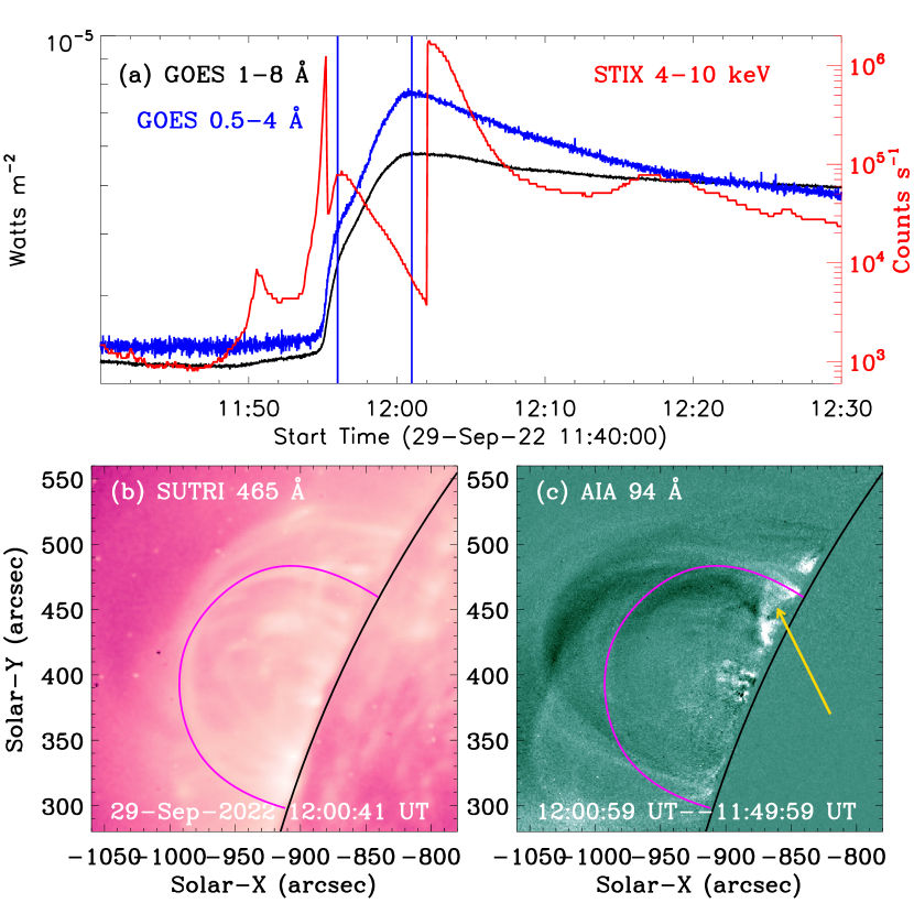
Figure 1: Overview of the solar flare and coronal loop on 2022 September 29. (a): Light curves integrated over the entire Sun at GOES 1$-$8 Å (black) and 0.5$-$4 Å (blue), and STIX 4$-$10 keV (red). The blue vertical lines mark two peaks of the solar flare in the GOES 0.5$-$4 Å flux. (b) & (c): Snapshots with a FOV of $\sim$330″$\times$330″in passbands of SUTRI 465 Å and AIA 94 Å. The magenta curve outlines a full loop profile, the gold arrow indicates the flare site, and the black line marks the solar limb. The whole evolution is shown in a movie of anim.mp4.

The coronal loops were simultaneously observed by SUTRI and SDO/AIA at wavelengths of EUV. SUTRI provides full-disk solar images at Ne VII 465 Å with a formation temperature of about 0.5 MK (Tian, 2017), the pixel scale is $\sim$1.23″, and the time cadence is roughly 30 s. Figure 1 (b) shows the EUV image taken by SUTRI at 12:00:41 UT, which shows several diffuse loops at the solar north-east limb, and the magenta line outlines one entire loop profile. Here, SUTRI successively observed the Sun from about 11:52 UT to 12:48 UT. SDO/AIA provides full-disk solar images at seven EUV wavelengths with a time cadence of 12 s and each pixel has a scale of 0.6″. Figure 1 (c) shows the base difference map (12:00:59 UT$-$11:49:59 UT) at AIA 94 Å, which shows bright emissions at one footpoint of the coronal loop, as indicated by the gold arrow. The bright emissions can be regarded as the major flare, which occurred at solar north-east limb, namely, N26E86. However, it is hard to see any signatures of coronal loops in the passband of AIA 94 Å, largely because it contains high-temperature plasma of $\sim$6.3 MK.

3 Data reductions and results

3.1 Overview of coronal loops

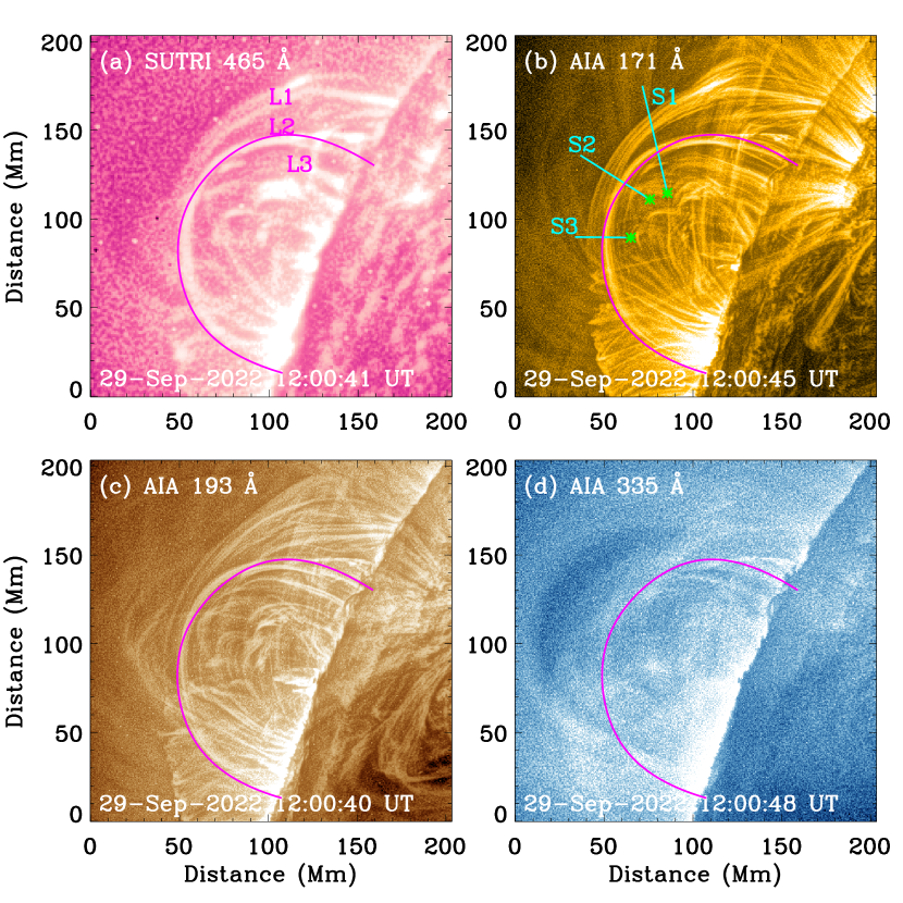
Figure 2: Multi-wavelength images with a same FOV seen in Figure 1 (b). They are observed by SUTRI at 465 Å (a), SDO/AIA at 171 Å (b), 193 Å (c), and 335 Å (d), and have been processed by the MGN technique. The magenta curve outlines the targeted loop. The straight cyan lines indicate the locations of three artificial slits (S1, S2, and S3), which are used to generate time-distance maps, and the green asterisks (‘$\ast$’) mark their starting points.

In Figure 1 (b), the coronal loops seen in the SUTRI map appear to be very fuzzy, mainly due to the diffuse nature of EUV emissions. In order to clearly identify these loop-like structures, an image-processing technique such as a multi-Gaussian normalization (MGN; Morgan & Druckmüller, 2014) was applied to the EUV image data observed by SUTRI and SDO/AIA. Thus, the coronal loops are evidently highlighted, as shown in Figure 2. A series of coronal loops can be simultaneously seen in passbands of SUTRI 465 Å, AIA 171 Å, and 193 Å. Herein, three coronal loops indicated by L1, L2, and L3 are chosen to investigate the transverse oscillation, since one of their footpoints is rooted in the flare region. The studied coronal loops seem to consist of several blended loops at AIA 171 Å and 193 Å, but those blended structures can not be distinguished at SUTRI 465 Å. Therefore, we regard these coronal loops as loop systems and do not consider their details such as fine-scale structures. On the other hand, only one coronal loop reveals a complete loop profile, that is, the loop apex and double footpoints can be clearly seen in EUV maps, which is regarded as the targeted loop (L2), as outlined by the magenta curve. While the other two loops (i.e., L1 and L3) just show one footpoint and the loop apex. Similarly to what has observed at AIA 94 Å, those coronal loops can not be well seen at AIA 335 Å, as shown in panel (d). Our observations suggest that the loop systems only contain plasma at low temperatures, that is, $<$2 MK.

The movie anim.mp4 shows the whole evolution of coronal loops and the associated flare from $\sim$11:52 UT to $\sim$12:18 UT. From this, we can find that at about 11:56 UT, a solar flare erupts close to the northern footpoint of the loop systems (see Fig. 1) and then it subsequently induces a transverse oscillation in the targeted loop system. Interestingly, the transverse oscillation appears to propagate along several loops, namely, from L3 through L2 to L1, and then it evolves to a standing kink oscillation. The transverse oscillation continues to exist until around 12:10 UT, when the coronal loops gradually disappear. In order to take a closer look the appearance of the transverse oscillation, we generated time-distance (TD) maps along three artificial straight slits (S1, S2, and S3), which are nearly perpendicular to the loop axis. This is indicated by three cyan lines in Figure 2 and the green stars (‘$\ast$’) mark their starting points.

3.2 Time-distance maps

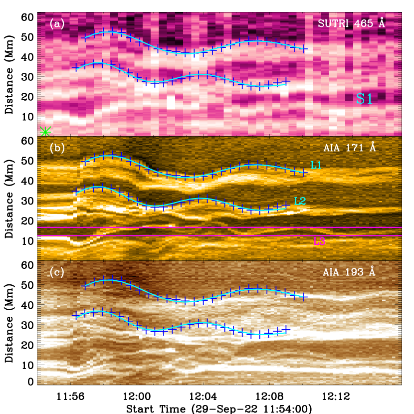
Figure 3: TD maps along slit S1 from 11:54 UT to 12:16 UT, which are made from image sequences at SUTRI 465 Å (a), AIA 171 Å (b), and 193 Å (c). These blue pluses (‘$+$’) highlight the skeletons of oscillating structures, whereas the cyan curves represent their best fitting results. The green asterisk (‘$\ast$’) marks the starting point of the TD map. Two magenta lines label another oscillating loop seen at AIA 171 Å.

Figure 3 presents TD maps for slit S1 that crosses the coronal loops in passbands of SUTRI 465 Å, AIA 171 Å and 193 Å, and the green symbol of ‘$\ast$’ indicates the zero-point of $y$-axis. In order to avoid any confusions, the slit S1 is selected at the northern locations where there are less overlaps with neighboring loops, and it is close to the solar flare. In these multi-wavelength TD maps, one can immediately notice that several transverse oscillations within at least two peaks. We first analyze the TD map at SUTRI 465 Å, because it shows two apparent transverse oscillations in loops L1 and L2 from about 11:56 UT to 12:10 UT. The oscillating locations of coronal loops are often determined by a Gaussian fitting method (e.g., Wang et al., 2012; Zhong et al., 2022). However, it is impossible to use this method if several overlapping loops simultaneously appear in the TD map (cf. Anfinogentov et al., 2015; Goddard et al., 2016). Therefore, we manually identified the edge of the oscillating loop (cf. Gao et al., 2022) along the transverse direction as the oscillatory locations, as marked by the blue pluses (‘+’) in panel (a). The two transverse oscillations appear to decay weakly, so a combination of a sine function, a decaying term and a linear trend is used to fit the loop oscillation (e.g., Nakariakov et al., 1999; Goddard et al., 2016; Su et al., 2018a), as shown by Equation 1:

$$y(t)=A\cdot\sin(\frac{2\pi}{P}\leavevmode\nobreak\ t+\psi)\cdot e^{-\frac{t}{\tau}}+k\cdot t+C,$$ (1)

Here, $A$ represents the initial displacement amplitude, $P$ and $\tau$ stand for the oscillation period and decaying time, $\psi$ and $C$ are initial phase and location of the transverse oscillation, and $k$ is a constant that refers to the drifting velocity of the oscillating loop system in the plane-of-sky. The fitting results are indicated by the cyan curve in Figure 3 (a), which match well with those identified skeletons of the oscillating loop system. Next, we could determine the velocity amplitude ($v_{m}$) by using the derivative of the displacement amplitude (cf. Gao et al., 2022; Li et al., 2022a), such as $v_{m}=2\pi\cdot\frac{A}{P}$. Some key parameters measured in the transverse oscillation are listed in Table 1.

Figure 3 (b and c) presents TD maps in passbands of AIA 171 Å and 193 Å, respectively. Besides the two transverse oscillations seen in the passband of SUTRI 465 Å, we can also see some other transverse oscillations, one such case is outlined by two magenta lines, that is, L3. However, the displacement profile is very different from a sine function, which could be considered as the signature of multiple harmonics and set it aside analysis later. Herein, we first focus our attention on the apparent transverse oscillations (L1 and L2), and these selected oscillating locations in panel a are directly overplotted in TD maps at AIA 171 Å and 193 Å, as shown by blue pluses in panels b and c. They appear to match well with the profile of transverse oscillations, suggesting a multi-thermal nature of the oscillating loop system. The best fitting results indicated by the cyan curves confirm that the transverse oscillation is basically a manifestation of decaying kink oscillation.

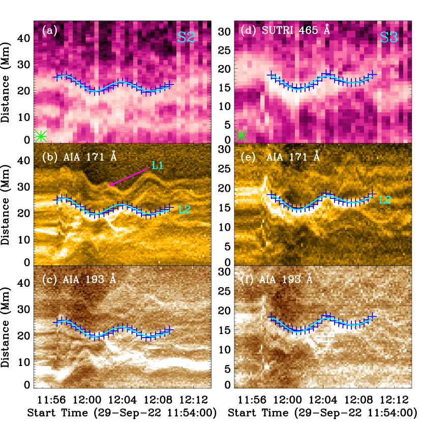
Figure 4: Similar to Figure 3, but they are generated from slits S2 (a$-$c) and S3 (d$-$f). The magenta arrow mark the transverse oscillation with multiple harmonics.

Figure 4 shows TD maps along two straight slits that cross the loop apex (S2) and the southern loop leg (S3), and they are almost perpendicular to the loop axis. Similarly to slit S1, an apparent transverse oscillation of loop L2 is simultaneously observed in passbands of SUTRI 465 Å, AIA 171 Å, and 193 Å. The oscillating locations are manually selected from the TD map at SUTRI 465 Å, and they could also appear in TD maps at AIA 171 Å and 193 Å, as indicated by blue pluses. The observations suggest that the transverse oscillation can be observed in multi-thermal loop system and no apparent phase difference appears at these three passbands. Table 1 also lists some key parameters for the transverse oscillation. Almost the same oscillation period implies that the transverse oscillation seen in three straight slits comes from the same oscillating loop system. We also notice that the transverse oscillation of loop L1 can only be seen at AIA 171 Å at the loop apex (S2), and it almost disappears at the southern loop leg (S3). Moreover, the displacement profile is also different from the sine function, implying a multi-harmonics wave, which is similar to the transverse oscillation of loop L3. The transverse oscillation of loop L3 can not be seen in slits S2 and S3, mainly because that the coronal loop L3 disappears. Thus, only the loop L2 that has an entire profile is detailed analyzed, as shown in table 1.

Table 1: Key parameters measured in the oscillating loop L2 at three positions.

	S1	S2	S3
$L$ (Mm)	221.3	221.3	221.3
$P$ (minutes)	6.32	6.38	6.32
$\tau$ (minutes)	9.6	10.5	10.6
$A$ (Mm)	12.5	7.9	6.1
$v_{\rm m}$ (km s-1)	207	130	101
$c_{\rm k}$ (km s-1)	1167	1156	1167
$n_{\rm i}$ (cm-3)	1.93$\times$109	1.66$\times$109	1.61$\times$109
$n_{\rm e}/n_{\rm i}$	0.30	0.35	0.36
$v_{\rm A}$ (km s-1)	941	950	962
$B$ (G)	21.3	20.0	19.9

In Figure 5, we show the best fitting results from the transverse oscillations that are generated from three straight slits in coronal loops of L1 and L2. The linear trend has been removed, so that they can be directly compared in the same window. Along the same slit S1, a visible time difference is seen when the transverse oscillation goes through loop L2 (black) and L1 (cyan), implying that the transverse oscillation is propagating along these two coronal loops. We can also find that the oscillation period in loop L1 is obviously longer than that in loop L2, because that the loop L1 is much longer than L2, as seen in Figure 2. In the same loop L2, the transverse oscillation at three different positions reaches the maximum (red solid line) and minimum (red dashed line) at almost the same time, suggesting that the loop system oscillates nearly in-phase along the loop length. The displacement amplitude of the transverse oscillation at the northern loop leg (S1) is obviously larger than that at the loop apex (S2) and at the southern loop leg (S3), because the solar flare that triggers the transverse oscillation erupted near the northern footpoints of the loop system, as shown in Figure 1. Our observations also suggest that the transverse oscillation of loop L2 is indeed the fundamental mode.

Figure 5: Best-fitting functions after removing the linear trend for the artificial slits S1 (black), S2 (magenta), and S3 (cyan) in coronal loops L1 and L2.

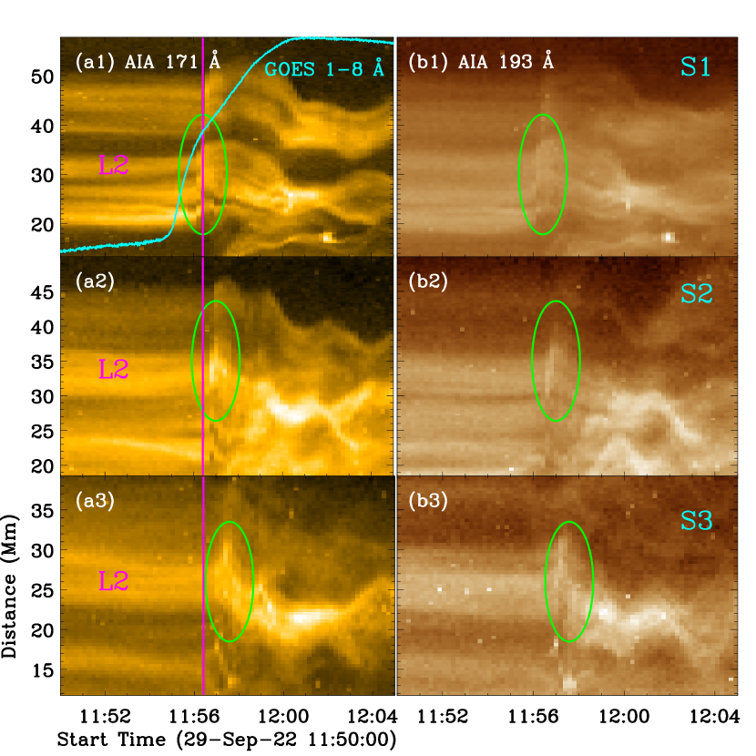
Figure 6: TD maps along slits S1$-$S3 from 11:50 UT to 12:05 UT, generated from data series at wavelengths of AIA 171 Å (a1$-$a3) and 193 Å (b1$-$b3). The magenta line marks a fixed time, and the green ellipse outlines the initial short pulse in different slits. The overplotted cyan line represents the GOES 1$-$8 Å flux.

Figure 5 demonstrates that the transverse oscillations in different loops are out of phase. However, it does not illustrate that the initial pulse triggered by the solar flare is a traveling wave, which is well seen in the movie anim.mp4. In order to provide the adequate demonstration, Figure 6 presents the TD plots taken from different slits, which are generated from AIA 171 Å and 193 Å image series during 11:50$-$12:05 UT. The overlaid cyan line is the GOES SXR light curve at 1$-$8 Å. We note that these TD images have been zoomed and have a common time axis. The coronal loop L2 is visible in these TD images at both AIA 171 Å and 193 Å, and it does not show any signature of transverse oscillations before the solar flare, for instance, from 11:50 UT to 11:55 UT. Then, a short transverse pulse appears in the coronal loop, which is accompanied by the flare eruption, as indicated by the green ellipse and cyan line. Next, the short pulse, which could be regarded as an initial transverse pulse, is evolved to a standing transverse oscillation of the coronal loop, as shown in Figure 3. Interestingly, the initial short pulse in the loop L2 appears later and later from slits S1 to S3, suggesting that there is a noticeable time delay between the appearance of the initial transverse pulse in different slits, as indicated by the green ellipse and magenta line in panels (a1)$-$(a3). The similar short transverse pulse with a time delay between different slits can also be seen at AIA 193 Å, as shown in panels (b1)$-$(b3). All those observations demonstrate that the initial short pulse is traveling along the coronal loop. That is to say, the initial pulse launched by the flare is a traveling wave.

3.3 DEM results

We further perform the differential emission measure (DEM) analysis for oscillating loop systems and the associated flare, as shown in Figure 7. In this study, an improved sparse-inversion code (Cheung et al., 2015) developed by Su et al. (2018b) was applied to determine the DEM($T$) distribution at every pixel, which is calculated from the SDO/AIA image data at six EUV passbands, that is, AIA 94 Å, 131 Å, 171 Å, 193 Å, 211 Å, and 335 Å. Their uncertainties are estimated from 100 Monte Carlo (MC) simulations for each pixel, that is, 3$\delta$ ($\delta$ refers to the standard deviation of 100 MC simulations). Panels (a) and (b) show narrow-band EM images that are integrated in temperature ranges of 0.5$-$1.8 MK and 8$-$20 MK, respectively. We immediately notice that coronal loops can be clearly seen at the lower temperature range between 0.5$-$1.8 MK (panel a), while the solar flare near the northern footpoint of the loop system is prominently visible at the higher temperature range of 8$-$20 MK, as marked by the gold arrow in panel (b). We also notice that only loop L2 has the whole loop-like profile in the EM map, which is consistent with SUTRI and SDO/AIA observations.

Figure 7 (c) shows the DEM profiles with error bars such as 3$\delta$ as a function of temperature. Here, we choose three positions (p1, p2, and p3) inside the oscillating loop (L2) and one position (p4) that is away from the oscillating loop (or background corona), as indicated by the blue boxes in panel (a). For clarity, only the error bars at the northern loop region (black line) and at the background position (magenta line) are shown in panel (c). The DEM profiles inside the oscillating loop (p1, p2, and p3) exhibit three apparent peaks at about 0.5 MK, 1.4 MK, and 2.5 MK, while the DEM profile at background corona (p4) only has two prominent peaks at around 0.4 MK and 2.5 MK. Moreover, the high-temperature peak at about 2.5 MK are roughly equal at those four positions, suggesting that it does indeed emit from the coronal emission of the diffuse background. On the other hand, the low-temperature peak at roughly 0.4 MK from the coronal background is significantly away from the peak at $\sim$0.5 MK. Based on these facts, we can conclude that the oscillating loop system of interest covers a temperature range from about 0.5 MK to 1.8 MK, as indicated by the yellow shadow. This agrees with our imaging observations, for instance, the oscillating loop system is clearly seen in passbands of SUTRI 465 Å ($\sim$0.5 MK), AIA 171 Å ($\sim$0.63 MK), and 193 Å ($\sim$1.58 MK).

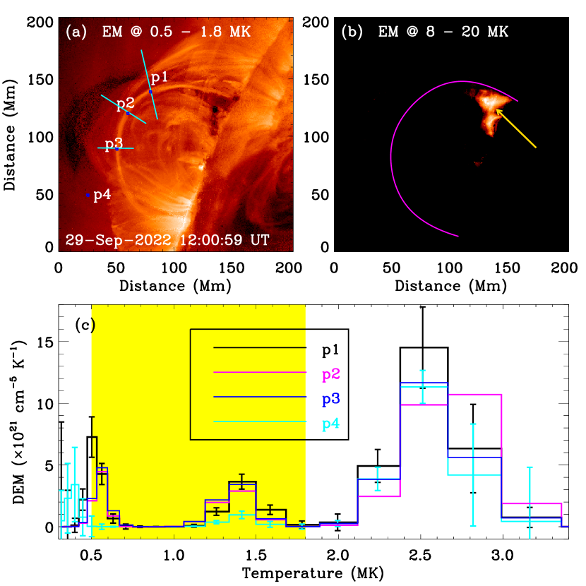
Figure 7: DEM analysis of the oscillating loop. (a) & (b): narrow-band EM images integrated in temperature ranges of 0.5$-$1.8 MK and 8$-$20 MK. (c): DEM profiles at three locations (P1, P2, and P3) inside the oscillating loop and at one location (P4) away from the oscillating loop. The yellow region outlines the EM and number density integration range for the oscillating loop. The error bars denote to the uncertainties ($3\delta$) of the DEM solution.

3.4 Coronal seismology

Generally, the transverse oscillation of an entire coronal loop is regarded as kink-mode wave because that the global sausage-mode wave requires for the very thick loop with quite denser plasmas (Nakariakov et al., 2003; Tian et al., 2016). Herein, we performed an MHD coronal seismology with Equations (2)$-$(4), based on the fundamental kink-mode oscillation of the coronal loop L2 (cf. Van Doorsselaere et al., 2014; Yuan & Van Doorsselaere, 2016; Long et al., 2017; Yang et al., 2020; Nakariakov et al., 2021).

$$c_{\rm k} = \frac{2L}{P},$$ (2)

$$v_{\rm A} = c_{\rm k}\cdot\sqrt{\frac{1+n{\rm{}_{e}}/n{\rm{}_{i}}}{2}},$$ (3)

$$B \approx v_{\rm A}\cdot\sqrt{\mu_{0}\leavevmode\nobreak\ n_{\rm i}\leavevmode\nobreak\ m_{\rm p}\leavevmode\nobreak\ \widetilde{\mu}},$$ (4)

Here $c_{\rm k}$ is the kink speed, $L$ refers to the length of oscillating loop, which can be determined by the distance between double footpoints when assuming a semi-circular shape for the coronal loop (cf. Tian et al., 2016; Li et al., 2022b), as indicated by the magenta curve in Figures 2 and 7. $n{\rm{}_{e}}$ and $n{\rm{}_{i}}$ represent external and internal number densities of the coronal loop, and they could be determined by the DEM results, such as $\sqrt{EM/w}$. $w$ is the integration length, which could consider as the full width at the half maximum of the coronal loop along its cross section, while it is the effective line-of-sight depth ($w\approx 4\times 10^{10}$ cm) in the background corona (Zucca et al., 2014; Su et al., 2018a). $v_{\rm A}$ and $B$ are the local Alfvén speed and magnetic field strength inside the oscillating loop system. Also, $\mu_{0}$ is the magnetic permittivity in vacuum, and $\widetilde{\mu}$ ($\approx$1.27) stands for the effective particle mass with respect to the proton mass ($m_{\rm p}$) in the solar corona (cf. White & Verwichte, 2012). The estimated parameters parameters are listed in Table 1.

3.5 Multiple harmonics

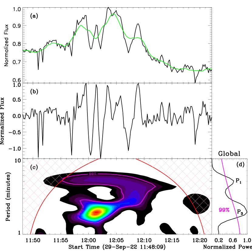
Figure 8: Wavelet analysis results. (a): Normalized time series integrated over two magenta lines in Figure 3, the overlaid green line is the slow-varying trend. (b) Normalized detrended time series. (c): Morlet wavelet power spectrum. (d): Global wavelet power spectrum. The magenta contours indicate a significance level of 99%.

In Figures 3 (b) and 4 (b), we can find that the displacement profile is very different from a sine, which is a strong signature of multiple harmonics of kink waves. Therefore, their periods are difficult to be determined by fitting a sine function, such as Equation 1. In order to identify the multiple periods, we performed a wavelet transform (Torrence & Compo, 1998) for the time series of oscillating loop L3, as shown in Figure 8. Panel (a) presents the raw time series integrated over two magenta lines in Figure 3 (b), and the time series has been normalized by its peak value. The overlaid green line represents the slow-varying trend, and the detrended time series is shown in panel (b). Here, we used a smooth window of 3 minutes to obtain the slow-varying trend (green line), because we thereby enhance the short-period oscillation and suppress the long-period trend (e.g., Kupriyanova et al., 2013; Kolotkov et al., 2016; Li et al., 2021; Li, 2022). Panels (c) and (d) shows the Morlet wavelet power spectrum and global wavelet power spectrum, respectively. From which, we can identify at least two periods with large uncertainties. Then, two dominant periods of 5.1 minutes (P₁) and 2.0 minutes (P₃) are determined by the double peaks above the 99% significance level in the global wavelet power spectrum. The period ratio (P₁/3P₃) is estimated to be 0.85, similarly to what has found between the fundamental and third harmonics in the decaying kink oscillation (cf. Duckenfield et al., 2019). So, the kink oscillation of loop L3 contains a third harmonic. Similarly, the standing kink oscillation of loop L1 along slit S2 also shows a strong signature of multiple harmonics, which is evolved from the traveling kink wave launched by a solar flare, as shown in Figure 3.

4 Conclusion and discussion

Using the EUV images taken by SUTRI and SDO/AIA, we investigate the decaying transverse oscillation of coronal loops. Combined observations from GOES and STIX reveal a major flare erupted close to one footpoint of those oscillating loops.

The observed oscillation of coronal loops is transverse in nature. It lasts for at least two wave periods while significantly decaying in amplitude; that is to say, the observed oscillation is basically an decaying kink wave. The initial displacement amplitude could be as large as 12.5 Mm and it decays rapidly, which is similar to previous findings about the decaying oscillation of coronal loops (e.g., Nakariakov et al., 1999; Goddard et al., 2016; Su et al., 2018a; Nechaeva et al., 2019; Ning et al., 2022), confirming that the transverse oscillation is indeed a decaying kink wave.

A solar flare is simultaneously observed near the northern footpoint of the oscillating loops. It is a C5.7 flare according to the GOES SXR classification, while it is an M4 class measured by the STIX 4$-$10 flux. This is because that the flare located at the solar limb from the Earth-orbit perspective, so only a partial emission could be received by GOES. STIX measured the whole flare emission at X-ray band at a different perspective. For this reason, STIX light curves are inserted attenuator. In any case, the solar flare is a major flare and it induces the decaying kink oscillation of coronal loops. This is also similar to pervious observations, for instance, the decaying oscillation is often driven by a solar erupted event such as a solar flare, EUV wave, or coronal jet or rain (Zimovets & Nakariakov, 2015; Shen et al., 2017; Reeves et al., 2020; Zhang et al., 2022).

The kink oscillation observed here is triggered by a major flare and it appears to propagate along several coronal loops. Figure 5 demonstrates the presence of phase difference in the kink wave between two coronal loops, such as L2 and L1, confirming that the kink oscillation propagates along different coronal loops, namely, from L3 through L2 to L1. While Figure 6 demonstrates that the initial short kink pulse launched by the major flare is indeed a traveling wave in one coronal loop. The traveling kink pulse is then evolved to a standing kink oscillation in the coronal loop. To the best of our knowledge, we observe the traveling kink oscillation evolving to the standing kink wave for the first time.

We investigated the standing kink oscillation in coronal loop L2 in detail because the oscillating loop has an entire profile with a loop length of $\sim$221.3 Mm by assuming a semi-circular loop shape (Figure 2). The oscillation period is measured to be about 6.3 minutes, which is consistent with previous findings in the period range of several minutes (e.g., Nakariakov et al., 1999; Anfinogentov et al., 2015; Su et al., 2018a; Nechaeva et al., 2019; Ning et al., 2022). The decaying time is estimated to 9.6$-$10.6 minutes and, thus, a ratio of $\sim$1.5$-$1.7 was found between the decaying time and oscillation period, similar to the average ratio found by Nechaeva et al. (2019). Both the initial displacement and velocity amplitude vary along the oscillating loop and they decrease when the oscillating slits are far away from the major flare. For instance, the displacement amplitude becomes from about 12.5 Mm at slit S1 to around 6.1 Mm at slit S3 (Table 1). We cannot find any signatures of phase difference among oscillating slits (S1, S2, and S3) at multi-wavelength channels, suggesting that the kink oscillation is indeed a fundamental mode. Based on the standing kink-mode wave, a seismological inference of the magnetic field is performed for the oscillating loop L2. The magnetic field strength inside the coronal loop is estimated to 19.9$-$21.3 G, which is consistent with previous estimations in coronal loops using MHD coronal seismology (Nakariakov & Ofman, 2001; Aschwanden et al., 2002; Yang et al., 2020; Li & Long, 2023). We want to stress that MHD coronal seismology was not performed for oscillating loops L1 and L3 because their loop profiles are incomplete, thus their loop lengths cannot be measured.

The standing kink oscillation of coronal loop L3 appears to contain multiple harmonics, since its displacement profile is very different from a sine function. Therefore, we performed a wavelet transform for the time series of the oscillating loop. Two dominant periods of 5.1 minutes (P₁) and 2.0 minutes (P₃) are identified in the wavelet spectra and their period ratio (P₁/3P₃) is estimated to 0.85, which agrees with previous findings in the decaying kink oscillation (cf. Duckenfield et al., 2019). The departure of period ratio from unity could be attributed to a density stratification of the oscillating loop. Our observation implies that the kink wave contains the fundamental and third harmonics. On the other hand, the standing kink oscillation in coronal loop L1 also reveals a strong signature of multiple harmonics, namely, non-sinusoidal displacement profile. It is first in the fundamental mode along slit S1, and then it contains multiple harmonics along slit S2. However, we could not see an oscillation signature at slit S3, because loop L1 disappears at slit S3. That is to say, it is evolved from the traveling kink wave. Finally, we want to stress that the oscillation period of the fundamental-mode kink wave becomes shorter and shorter from oscillating loops L1 to L3, which could be attributed to the observational fact that the oscillation period of kink waves is strongly dependent on the loop length (e.g., Anfinogentov et al., 2015; Goddard et al., 2016; Li & Long, 2023).

5 Summary

Based on the observation measured by SUTRI, SDO/AIA, GOES, and STIX, we explored the decaying kink oscillation in three coronal loops. Our main results are summarized as follows:

1. We first observe the evolution of a traveling kink pulse to a standing kink wave in the coronal loop that has been triggered by a major flare.

2. Based on the kink-mode wave, the Alfvén speed and magnetic field strength inside the oscillating loop were estimated to be about 950 km s^-1 and 20 G, respectively.

3. The fundamental and third harmonics of kink wave were simultaneously detected in the oscillating loop.