KMT-2022-BLG-2397: Brown Dwarf at the Upper Shore of the Einstein Desert

Abstract

We measure the Einstein radius of the single-lens microlensing event KMT-2022-BLG-2397 to be $\theta_{\rm E}=24.8\pm 3.6\,\mu{\rm as}$, placing it at the upper shore of the Einstein Desert, $9\lesssim\theta_{\rm E}/\mu{\rm as}\lesssim 25$, between free-floating planets (FFPs) and bulge brown dwarfs (BDs). In contrast to the six BD ($25\lesssim\theta_{\rm E}\lesssim 50$) events presented by Gould et al. (2022), which all had giant-star source stars, KMT-2022-BLG-2397 has a dwarf-star source, with angular radius $\theta_{*}\sim 0.9\,\mu{\rm as}$. This prompts us to study the relative utility of dwarf and giant sources for characterizing FFPs and BDs from finite-source point-lens (FSPL) microlensing events. We find “dwarfs” (including main-sequence stars and subgiants) are likely to yield twice as many $\theta_{\rm E}$ measurements for BDs and a comparable (but more difficult to quantify) improvement for FFPs. We show that neither current nor planned experiments will yield complete mass measurements of isolated bulge BDs, nor will any other planned experiment yield as many $\theta_{\rm E}$ measurements for these objects as KMT. Thus, the currently anticipated 10-year KMT survey will remain the best way to study bulge BDs for several decades to come.

1 Introduction

Isolated dark objects can only be studied with gravitational microlensing. In principle, their masses, distances, and transverse velocities can be determined by measuring seven parameters, which can be summarized as five quantities (two of which are vectors). These are the Einstein timescale ($t_{\rm E}$), the angular Einstein radius ($\theta_{\rm E}$), the microlens parallax vector (${\mbox{\boldmath$\pi$}}_{\rm E}$), and the source parallax and proper motion, ($\pi_{S}$ and ${\mbox{\boldmath$\mu$}}_{S}$). Here,

$$t_{\rm E}={\theta_{\rm E}\over\mu_{\rm rel}};\qquad\theta_{\rm E}=\sqrt{\kappa M\pi_{\rm rel}};\qquad\kappa\equiv{4\,G\over c^{2}\,{\rm au}}\simeq 8.14\,{{\rm mas}\over M_{\odot}},$$ (1)

and

$${\mbox{\boldmath$\pi$}}_{\rm E}=\pi_{\rm E}{{\mbox{\boldmath$\mu$}}_{\rm rel}\over\mu_{\rm rel}};\qquad\pi_{\rm E}\equiv{\pi_{\rm rel}\over\theta_{\rm E}},$$ (2)

where $M$ is the lens mass, ($\pi_{\rm rel},{\mbox{\boldmath$\mu$}}_{\rm rel}$) are the lens-source relative (parallax, proper-motion), and $\mu_{\rm rel}\equiv|{\mbox{\boldmath$\mu$}}_{\rm rel}|$. Then, the lens mass, distance $D_{L}$, and transverse velocity ${\bf v}_{\perp}$ are given by

$$M={\theta_{\rm E}\over\kappa\pi_{\rm E}};\qquad D_{L}={{\rm au}\over\pi_{\rm rel}+\pi_{S}};\qquad{\bf v}_{\perp}=D_{L}({\mbox{\boldmath$\mu$}}_{S}+{\mbox{\boldmath$\mu$}}_{{\rm rel},{\rm hel}}),$$ (3)

where

$$\pi_{\rm rel}=\theta_{\rm E}\pi_{\rm E};\qquad{\mbox{\boldmath$\mu$}}_{{\rm rel},{\rm hel}}={\mbox{\boldmath$\mu$}}_{\rm rel}+{\pi_{\rm rel}\over{\rm au}}{\bf v}_{\oplus,\perp};\qquad{\mbox{\boldmath$\mu$}}_{\rm rel}={{\mbox{\boldmath$\pi$}}_{\rm E}\over\pi_{\rm E}}\,{\theta_{\rm E}\over t_{\rm E}}$$ (4)

and where ${\bf v}_{\oplus,\perp}$ is Earth’s orbital velocity at the peak of the event projected on the sky.

After 30 years of dedicated surveys that have cataloged more than 30,000 microlensing events, such complete characterizations have been carried out for exactly one isolated dark object: OGLE-2011-BLG-0462/MOA-2011-BLG-191, which is a black hole (BH, Sahu et al. 2022; Lam et al. 2022) with mass $M=7.88\pm 0.82\,M_{\odot}$, distance $D_{L}=1.62\pm 0.15\,{\rm kpc}$, and $v_{\perp}=43.4\pm 3.8\,{\rm km}\,{\rm s}^{-1}$, with a direction (Galactic North through East) of $\phi=-17^{\circ}$ (Mróz et al., 2022).

If ${\mbox{\boldmath$\mu$}}_{S}$ cannot be measured or if the direction of ${\mbox{\boldmath$\mu$}}_{\rm rel}$ is ambiguous (and if $\pi_{S}$ can be measured or adequately estimated), then one loses the measurement of ${\bf v}_{\perp}$ but still retains those of $M$ and $D_{L}$. There are three other such mass measurements of isolated dark objects, all brown dwarfs (BDs). These are OGLE-2007-BLG-224, with $M=58\pm 4\,M_{\rm jup}$, $D_{L}=0.52\pm 0.04\,{\rm kpc}$ (Gould et al., 2009) and OGLE-2015-BLG-1268, with $M=47\pm 7\,M_{\rm jup}$ and $D_{L}=5.9\pm 1.0\,{\rm kpc}$ (Zhu et al., 2016), and OGLE-2017-BLG-0896 (Shvartzvald et al., 2019), with $M=19\pm 2\,M_{\rm Jup}$, and $D_{L}=4.0\pm 0.2\,{\rm kpc}$.

For OGLE-2007-BLG-224, the lens is so much closer to the Sun than the source and has such high $\mu_{{\rm rel},{\rm hel}}=43\,{\rm mas}\,{\rm yr}^{-1}$, that ${\mbox{\boldmath$\mu$}}_{S}$ plays very little role in assessing the kinematics of the lens. Moreover, its source star is in the Gaia (Gaia Collaboration et al., 2016, 2018) DR3 catalog. Although it does not have a proper-motion measurement in DR3, its proper motion could be measured in future Gaia data releases. However, the other two events both have ambiguous directions for ${\mbox{\boldmath$\mu$}}_{\rm rel}$, so the transverse velocities will remain unknown even if ${\mbox{\boldmath$\mu$}}_{S}$ is later measured.

These four mass-distance determinations of isolated dark objects nicely illustrate the three methods that have been used to date to measure ${\mbox{\boldmath$\pi$}}_{\rm E}$, as well as two of the three methods that have been used to measure $\theta_{\rm E}$. For OGLE-2011-BLG-0462, ${\mbox{\boldmath$\pi$}}_{\rm E}$ was measured by annual parallax (Gould, 1992), while $\theta_{\rm E}$ was measured using astrometric microlensing (Walker, 1995; Hog et al., 1995; Miyamoto & Yoshii, 1995). For OGLE-2007-BLG-224, ${\mbox{\boldmath$\pi$}}_{\rm E}$ was measured by terrestrial parallax (Holz & Wald, 1996; Gould, 1997), while $\theta_{\rm E}$ was measured from finite-source effects as the lens transited the source (Gould, 1994a; Witt & Mao, 1994; Nemiroff & Wickramasinghe, 1994). For OGLE-2015-BLG-1268 and OGLE-2017-BLG-0896, ${\mbox{\boldmath$\pi$}}_{\rm E}$ was measured by satellite parallax (Refsdal, 1966; Gould, 1994b), while $\theta_{\rm E}$ was again measured from finite-source effects. The other method that has been used to measure $\theta_{\rm E}$ (but not yet applied to isolated dark objects) is interferometric resolution of the microlensed images (Delplancke et al., 2001; Dong et al., 2019; Cassan et al., 2021).

For completeness, we note that there are two other events with mass measurements whose BD nature could be confirmed (or contradicted) by future adaptive-optics (AO) observations on extremely large telescopes (ELTs). One of these is OGLE-2015-BLG-1482 (Chung et al., 2017), which has two solutions, one with a BD lens ($M=57\,M_{\rm jup}$, $D_{L}=7.5\,{\rm kpc}$) and the other with a stellar lens ($M=100\,M_{\rm jup}$, $D_{L}=7.2\,{\rm kpc}$). If the latter is correct, then $\mu_{\rm rel}\simeq 9\,{\rm mas}\,{\rm yr}^{-1}$, so that at first AO light on ELTs, plausibly 2030, the lens and the clump-giant source will be separated by about 135 mas, which would permit the lens to be detected for the stellar-mass solution. Hence, if the lens is not detected, then the BD solution will be correct. The other is OGLE-2016-BLG-1045 (Shin et al., 2018), which has a unique solution at the star-BD boundary, ($M=0.08\pm 0.01\,M_{\odot}$, $D_{L}=5.02\pm 0.14\,{\rm kpc}$). If the lens is a star (and so is luminous), then it can be detected in AO observations after it is sufficiently separated from the source. However, because the source is a giant, the proper motion is only $\mu_{\rm rel}\sim 7\,{\rm mas}\,{\rm yr}^{-1}$, and a stellar lens must be detectable down to very faint magnitudes in order to confirm a possible BD, this may not be feasible immediately after first AO light on ELTs, depending on the performance of these instruments.

As we will discuss in Section 7, there are good long-term prospects for obtaining complete solutions for isolated dark objects in both regimes, i.e., both dark massive remnants and dark substellar objects. However, while the new instruments required to make progress in the high-mass regime are already coming on line, those required for the low-mass regime are several years to several decades away. Hence, for the present, techniques that yield only partial information are still needed to probe substellar-object populations.

Two such methods have been developed to date: analysis of the $t_{\rm E}$ distribution of detected microlensing events (Sumi et al., 2011; Mróz et al., 2017), and analysis of the $\theta_{\rm E}$ (and $\mu_{\rm rel}=\theta_{\rm E}/t_{\rm E}$) distributions of the subset of single-lens events that have such measurements, so-called finite-source point-lens (FSPL) events (Kim et al., 2021; Gould et al., 2022). Each approach has its advantages and disadvantages. Before comparing these, it is important to note that both approaches must rely on Galactic models to interpret their results because the masses and distances of individual objects cannot be determined from either $t_{\rm E}$ or $(\theta_{\rm E},\mu_{\rm rel})$ measurements alone.

The great advantage of the $t_{\rm E}$ approach is that very large samples of events are available, even accounting for the fact that only fields subjected to high-cadence observations can contribute substantially to the detection of low-mass objects. In particular, Mróz et al. (2017) leveraged this advantage to make the first detection of six members of a population of short, $t_{\rm E}\sim 0.5\,$day, events, which was separated by a gap from the main distribution of events, and which they suggested might be due to a very numerous class of free-floating planets (FFPs). However, while this new population is clearly distinct in $t_{\rm E}$ space, it is difficult to constrain its properties based on $t_{\rm E}$ measurements alone. In particular, there is no reason, a priori, to assume that its density distribution follows that of the luminous stars that define the Galactic model. The events just on the larger-duration side of the $t_{\rm E}$ gap are almost certainly dominated by the lowest-mass part of the stellar-BD population. Because the luminous-star component of this distribution can be studied by other techniques, models of the luminous component can provide powerful constraints that facilitate disentangling the BD signal within the $t_{\rm E}$ distribution, which is necessarily a convolution of BD and stellar components. Nevertheless, because the BD component may differ substantially in the Galactic bulge and/or the distant disk relative to the local one that can be directly studied, it may be difficult to disentangle the different populations, given that there is little information on the mass and distance of each lens and that these are convolved with the kinematics. See Equation (1).

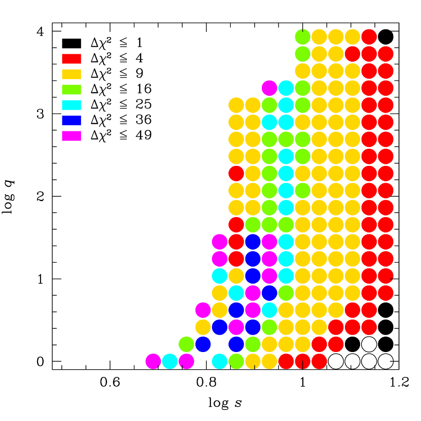
Figure 4: Grid search for binary-lens solutions, with resulting $\Delta\chi^{2}=\chi^{2}({\rm binary})-\chi^{2}({\rm FSPL})$ coded by point type and color. Filled symbols indicate $\Delta\chi^{2}>0$, while open symbols indicate $\Delta\chi^{2}<0$. The color coding is indicated in the legend, while the blank regions have $\Delta\chi^{2}>49$. The grid search is over three variables $(s,q,\alpha)$ but only the best $\chi^{2}(s,q)$ (i.e., marginalized over $\alpha$) is shown. Values $\log s\leq 0.8$ ($s<6.3$) are clearly ruled out, but there is an “island” of allowed solutions just above this value. Full exploration of this island yields $\Delta\chi^{2}\sim-2$ for 3 dof, which is not significant.

The $\theta_{\rm E}$ approach, by contrast, has several orders of magnitude fewer events. For example, Gould et al. (2022) recovered just 30 giant-source FSPL events from 4 years of Korean Microlensing Telescope Network (KMTNet, Kim et al. 2016) data compared to an underlying sample of about 12,000 events. Nevertheless, this approach has several major advantages, particularly in the study of low-mass objects. The most important is that for a source of fixed angular radius, $\theta_{*}$, the rate of FSPL events scales as $\theta_{*}$ (i.e., is independent of lens mass, Gould & Yee 2013), whereas the rate of microlensing events in general scales $\propto\theta_{\rm E}\sim\sqrt{M}$. Thus, among the 30 FSPL events found by Gould et al. (2022), four were from the same FFP population from which Mróz et al. (2017) identified six members from a much larger sample. As in the Mróz et al. (2017) $t_{\rm E}$ sample, these were separated by a gap from the main body of detections, which spans a factor of three in $\theta_{\rm E}$ and which Kim et al. (2021) dubbed the “Einstein Desert”. See Figure 4 from Gould et al. (2022).

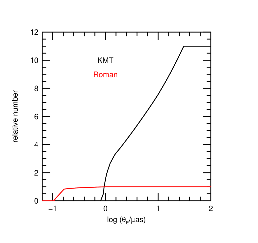
Figure 9: Relative sensitivity to FSPL events of the Roman and KMT surveys as a function of Einstein radius $\theta_{\rm E}$. The asymptotic ratio of 11 at the right reflects the fact that 11 times more events take place in the KMT purview, while essentially all FSPL events with $\theta_{\rm E}\sim 100\,\mu{\rm as}$ are detected in either survey. For smaller $\theta_{\rm E}$, Roman continues to detect almost all events down to almost $\theta_{\rm E}\sim 0.1\,\mu{\rm as}$, whereas KMT sensitivity continuously declines over this range, dropping to zero near $\theta_{\rm E}\sim 1\,\mu{\rm as}$. This points to $0.1\lesssim\theta_{\rm E}/\mu{\rm as}\lesssim 1$ as a key “discovery space” for Roman, a region that could contain a vast population of FFPs.

A second major advantage, which follows from the same $\propto\theta_{*}$ scaling, but is perhaps less obvious, is that FSPL events are heavily weighted toward bulge lenses (at least for those above the Einstein Desert). This is because, just as $\theta_{\rm E}\propto\sqrt{M}$, it is equally the case that $\theta_{\rm E}\propto\sqrt{\pi_{\rm rel}}$. This effect can be seen in Figure 9 of Gould et al. (2022). Hence, in an FSPL sample (above the Einstein Desert), one is primarily studying bulge lenses, which renders the interpretation cleaner.

The combination of these two effects implies that the six events found by Gould et al. (2022) in the range $25<\theta_{\rm E}/\mu{\rm as}<50$ are likely to be overwhelmingly bulge BDs, with possibly some contamination by very low-mass stars. That is, scaling to a characteristic bulge-lens/bulge-source relative parallax $\pi_{\rm rel}\sim 10\,\mu{\rm as}$ (corresponding to a distance along the line of sight $D_{LS}\equiv D_{S}-D_{L}\sim 650\,{\rm pc}$),

$$M={\theta_{\rm E}^{2}\over\kappa\pi_{\rm rel}}=32\,M_{\rm jup}\biggl{(}{\theta_{\rm E}\over 50\,\mu{\rm as}}\biggr{)}^{2}\biggl{(}{\pi_{\rm rel}\over 10\,\mu{\rm as}}\biggr{)}^{-1}.$$ (5)

This brings us to the next advantage, which is that it is relatively straightforward to vet an FSPL sample of BD candidates for stellar “contamination”. That is, in contrast to the underlying sample of events (with only $t_{\rm E}$ measurements), $\mu_{\rm rel}$ is known for each FSPL event. Hence, it is possible to know in advance both how long one must wait for AO observations that could potentially see the lens (assuming that it is luminous) and what is the annulus around the source that must be investigated in the resulting image. Such AO followup observations would also reveal whether the BD was truly isolated. In fact, Shan et al. (2021) carried out this test for OGLE-2007-BLG-224 and ruled out the possibility of a main sequence lens.

Moreover, because there are relatively few BD/stellar FSPL objects in the Gould et al. (2022) sample, which likely includes roughly 8 BDs, one could afford to probe a substantially larger fraction of this sample than just the events that are most likely to be BDs. The lenses that were thereby revealed to be luminous would in themselves be useful because they could confirm (or contradict) the predictions of the Galactic model.

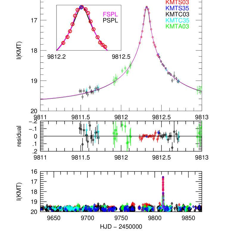
Figure 1: Data (colored points) and single-lens single-source models for KMT-2022-BLG-2397 that do include (FSPL) or do not include (PSPL) finite-source effects. The bottom panel shows the whole 2022 season, while the top panel shows the 2 days around the peak. The middle panel shows the residuals to the FSPL fit. The inset is a zoom of the peak region, in which it is clear that the PSPL model (green) fails to match the data. Formally, $\Delta\chi^{2}=128$.

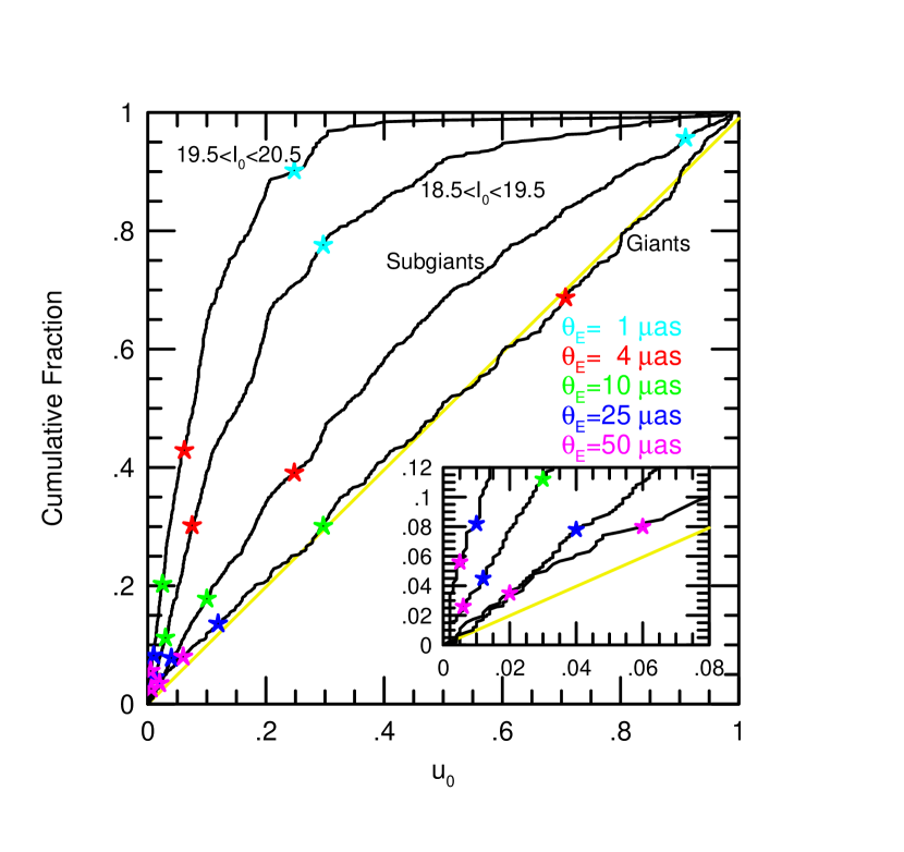
Figure 5: Cumulative distributions of 2019 KMT events as a function of impact parameters $0<u_{0}\leq 0.99$ as derived from the KMT web page for four sub-populations, including two groups of main-sequence stars ($19.5<I_{0}<20.5$ and $18.5<I_{0}<19.5$), subgiants ($16.5<I_{0}<18.5$), and giants ($13.0<I_{0}<16.5$). The yellow line shows the expected distribution for events unaffected by selection bias, which is a good match to the giants. The other populations show increasing evidence of magnification bias. The colored points are at the $u_{0}$ values that generate the same magnification as an FSPL event with $\rho=\theta_{*}/\theta_{\rm E}$, i.e., $u_{0}^{2}=\sqrt{4+\rho^{2}}-2$. Here, we adopt $\theta_{*}=(0.5,0.6,2,6)\,\mu{\rm as}$ for the four sub-populations, while the $\theta_{\rm E}$ values are given in the legend. For BDs ($25\lesssim\theta_{\rm E}/\mu{\rm as}\lesssim 50$), all populations are in the linear regime (see inset), so magnification bias plays essentially no role. This remains basically the case for FFPs similar to those in the Gould et al. (2022) giant-source study ($4\lesssim\theta_{\rm E}/\mu{\rm as}\lesssim 10$). However, for substantially smaller $\theta_{\rm E}\sim 1\,\mu{\rm as}$, magnification bias plays a major role (cyan points).

That said, this third advantage is somewhat compromised for the giant-source FSPL sample of Gould et al. (2022) because even the 10–15 year interval between the events and ELT AO first light may not be enough for the source and lens to separate sufficiently to probe to the hydrogen burning limit. Given the source-magnitude distribution shown in Figure 1 of Gould et al. (2022), contrast ratios of $\gtrsim 10^{4}$ in the $K$ band would be required. While we cannot be too precise about instruments that have not yet been built, scaling from AO on Keck, this will probably require separations of $\gtrsim 100\,{\rm mas}$ even on the 39m European ELT. From Figure 5 of Gould et al. (2022), one sees that this will not occur until well after 2030 for many of the BD candidates.

Here, we present KMT-2022-BLG-2397, the second FSPL bulge-BD candidate with a dwarf-star source. Because this source is about 4 mag fainter than the clump, the required contrast ratio will be about 250 rather than $\gtrsim 10^{4}$. Based on its measured proper motion, $\mu_{\rm rel}=6.7\pm 1.0\,{\rm mas}\,{\rm yr}^{-1}$, the source and lens will be separated by about 50 mas in 2030 and 85 mas in 2035. The first will be sufficient to probe for typical luminous companions, while the second will be good enough to probe to the hydrogen-burning limit.

After presenting the analysis of this event, we discuss the prospects for identifying a larger sample of bulge-BD candidates with dwarf-star sources in context of the ongoing development of other possible competing methods to probe bulge BDs. Relatedly, after the initial draft of this paper was essentially complete, Koshimoto et al. (2023) and Sumi et al. (2023) posted two papers on an FSPL search carried out based on 9 years of MOA data and combining measurements of the $t_{\rm E}$ and $\theta_{\rm E}$ distributions. This search is highly relevant but does not materially impact our investigations. Hence, we discuss this work in detail in Section 7.4, but do not otherwise modify the main body of the paper (except for adding footnotes 4 and 6).

2 Observations

KMT-2022-BLG-2397 lies at (RA, Decl)${}_{J2000}=$(18:02:19.73,$-26$:53:28.10), corresponding to $(l,b)=(+3.64,-2.15)$. It was discovered using the KMT EventFinder (Kim et al., 2018a) system, which is applied post-season to the data taken with KMTNet’s three identical telescopes in Australia (KMTA), Chile (KMTC), and South Africa (KMTS). These telescopes have 1.6m mirrors and are equipped with $4\,{\rm deg}^{2}$ cameras. The observations are primarily in the $I$ band, but after every tenth such exposure, there is one in the $V$ band for the purpose of measuring the source color. The event lies in the overlap of KMT fields BLG03 and BLG35. For KMTC, these are observed at nominal cadences of $\Gamma=2\,{\rm hr}^{-1}$ and $\Gamma=0.4\,{\rm hr}^{-1}$, while for KMTS and KMTA, $\Gamma=3\,{\rm hr}^{-1}$ and $\Gamma=0.3\,{\rm hr}^{-1}$ for the respective fields. The data were initially reduced using the KMT pySIS (Albrow et al., 2009) pipeline, which is a specific realization of difference image analysis (DIA, Tomaney & Crotts 1996; Alard & Lupton 1998) tailored to the KMT data. They were re-reduced for publication using a tender loving care (TLC) version of pySIS (Yang et al. 2023, in prep).

Note that KMT-2022-BLG-2397 was not discovered by the in-season KMT AlertFinder (Kim et al., 2018b) system, which is operated once per weekday during most of the observing season and which is responsible for a substantial majority of all KMT event detections. As the purpose of this system is to identify events that are suitable for follow-up observations, it is tuned to rising events. The KMT-2022-BLG-2397 microlensing event was undetectable in the data until about one hour before peak. Hence, by the time it would normally have been subjected to AlertFinder analysis 6 hours later, it was already falling. Moreover, this was on a Sunday, so there was no actual analysis until Monday, when the event was essentially at baseline.

The KMTA data from BLG35 are of very poor quality and so are not included in the analysis. This exclusion has almost no effect for three reasons. First, the cadence for BLG03 is 10 times higher. Second, the KMTA data fall on an unconstraining part of the light curve. Third, conditions were poor on the one night when KMTA data would be relevant at all.

KMT-2022-BLG-2397 was recognized as a potentially interesting event during the initial review of the roughly 500 new EventFinder events from 2022.

3 Light Curve Analysis

Figure 1 shows a very short, classic FSPL event, in which the rising light curve first steepens as the lens starts to transit the source, and then flattens over peak, followed by a symmetric decline. The residuals show no systematic deviations over the peak. The peak is captured entirely by KMTS data, with 19 points from BLG03 and 2 from BLG35, over a total of 5.6 hours. The inset shows a point-source point-lens (PSPL) fit in black for comparison. It clearly cannot match the sharp rise and fall on the wing, nor the flattening over the peak, of the data (and the FSPL model). Formally it is rejected by $\Delta\chi^{2}=128$. In addition, the source magnitude according to the PSPL model (when converted to the calibrated OGLE-III system, see Section 4) is substantially brighter than the baseline object from the OGLE-III catalog. This is further evidence against the PSPL model, but a full explanation would involve additional complications, and as it is not necessary for the rejection of the PSPL model, we do not pursue it.

Table 1 shows the five fit parameters of the model $(t_{0},u_{0},t_{\rm E},\rho,I_{S})$. Here $t_{0}$ is the time of the peak, $u_{0}$ is the impact parameter normalized to $\theta_{\rm E}$, $\rho=\theta_{*}/\theta_{\rm E}$, and $I_{S}$ is the source magnitude in the KMTC03 system. In addition, we show the four “invariant” parameters, $t_{\rm eff}\equiv u_{0}t_{\rm E}$, $t_{*}\equiv\rho t_{\rm E}$, $z_{0}\equiv u_{0}/\rho$, and $f_{S}t_{\rm E}$, where $f_{S}\equiv 10^{-0.4(I_{S}-18)}$.

In fact, in order to emphasize several key points, we have put the nonstandard parametrization $(t_{0},t_{\rm E},t_{\rm eff},f_{S}t_{\rm E})$ in the top rows of Table 1. The first point is that the unit of all five of these parameters is time. Second, the last three of these parameters each have errors of $\lesssim 2.5\%$ compared to the $\sim 9\%$ errors of the corresponding standard parameters $(u_{0},\rho,f_{S})$ from which they are derived. Thus, these larger errors are rooted in their correlation with $t_{\rm E}$, which is 8%. Finally, while the error in $t_{0}$ appears to be impressively small (just 30 seconds), in fact this does not enable any precision physical measurements. For example, during this seemingly short interval, the lens sweeps across the observer plane by a distance $({\rm au}/\pi_{\rm rel})\mu_{\rm rel}\sigma(t_{0})\sim 0.15\,R_{\oplus}(\pi_{\rm rel}/{\rm mas})^{-1}$. Hence, for the great majority of lenses, which have $\pi_{\rm rel}\lesssim 0.1\,{\rm mas}$, there could not be even a $1\,\sigma$ terrestrial parallax measurement (even assuming that the event had been observed over peak at another Earth location).

We also note that while the error in the impact parameter $u_{0}$ is 9%, its value relative to the source size, i.e., $z_{0}\equiv u_{0}/\rho$ is measured to 2.4%.

4 Source Properties

Because $\rho$ was measured, we can, in principle, use standard techniques (Yoo et al., 2004) to determine the angular source radius, $\theta_{*}$ and so infer $\theta_{\rm E}$ and $\mu_{\rm rel}$:

$$\theta_{\rm E}={\theta_{*}\over\rho};\qquad\mu_{\rm rel}={\theta_{\rm E}\over t_{\rm E}}.$$ (6)

In this approach, one measures the offset $\Delta[(V-I),I]$ of the source star relative to the clump, add in the known dereddened color and magnitude of the clump $[(V-I),I]_{\rm cl,0}=(1.06,14.34)$ (Bensby et al., 2013; Nataf et al., 2013) to obtain the dereddened position of the source $[(V-I),I]_{\rm s,0}=[(V-I),I]_{\rm cl,0}+\Delta[(V-I),I]_{S,0}$. Then one applies a color/surface-brightness relation to determine $\theta_{*}$. In our case, we use the $V/K$ relations of Kervella et al. (2004) by first applying the $VIK$ color-color relations of Bessell & Brett (1988) to transform from $V/I$ to $V/K$.

However, the practical implementation of this approach poses greater challenges than is usually the case. The first challenge is that there is only one well-magnified $V$-band measurement to be used to measure $(V-I)_{S}$. This is partly a consequence of the fact that the event is extremely short ($t_{\rm E}\sim 1.3\,$day), that the source is faint $(I_{S}\sim 21)$, that it is substantially magnified for only a few hours, and that only 9% of the observations are in the $V$-band. However, in this case, these problems were exacerbated by what is essentially a bug in the observation-sequence script. The script alternates between a series (roughly one per night) of 176 observations that contain no BLG02 or BLG03 $V$-band observations and another series that contains one $V$-band observation per five $I$-band observations. In the great majority of cases, this makes essentially no difference because events in these fields also lie in BLG42 or BLG43, for which the pattern is reversed. And the great majority of the events that do not have such overlap remain near their peak magnification for many days. However, neither of these “failsafes” applied to KMT-2022-BLG-2397. Fortunately, one of the two BLG35 $I$-band observations was complemented by a $V$-band observation, and it happened to be right at the peak of the event. See Figure 1. This permits a measurement of the $(V-I)$ color, but without a second observation as a check. While there is an additional $V$-band observation from KMTC03 on the falling wing, the source was by that time too faint to permit a useful measurement.

A second major issue is that there is an unusually large amount of differential reddening in the neighborhood of the source. Figure 2 shows the clump region of the OGLE-III (Szymański et al., 2011) color-magnitude diagram (CMD), centered on the event and with radii of $200^{\prime\prime}$, $100^{\prime\prime}$, $60^{\prime\prime}$, and $30^{\prime\prime}$. The red circle indicates our ultimately-adopted position of the clump centroid (see below), while the magenta line in the upper-left panel gives our estimate of the reddening track. It has a slope of $R_{VI}\equiv\Delta A_{I}/\Delta E(V-I)=1.52$.

Within the $200^{\prime\prime}$ circle, the clump is quite extended and its centroid is substantially brighter and bluer than our ultimately-adopted position. For the $100^{\prime\prime}$ circle, the clump remains extended, but its centroid is closer to our adopted position. For the $60^{\prime\prime}$ circle, the clump centroid is close to our adopted position, although it is already very thinly populated. The $30^{\prime\prime}$ circle confirms that the clump centroid is well localized near our adopted position, although one would not try to measure the clump position based on this panel alone.

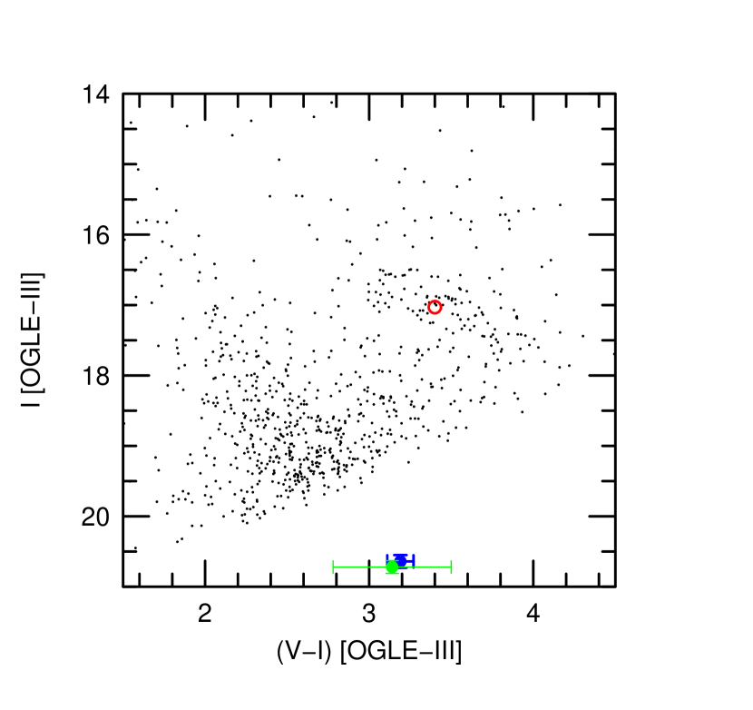
Figure 3: Full CMD within $60^{\prime\prime}$ of KMT-2022-BLG-2397. The red circle is the clump centroid (same as in Figure 2). The blue and green points are two independent measurements of the source color and magnitude, from KMTS35 and KMTC01, respectively. The latter provides a truly independent measurement of $I_{S}$ but only qualitative confirmation of $(V-I)_{S}$.

Figure 3 shows the full CMD within the $60^{\prime\prime}$ circle. The blue and green points represent the position of the source as determined from the KMTS35 and KMTC03 fields respectively. The latter only qualitatively confirms the source color, but it does give an independent measurement of the source magnitude.

We determined the source CMD parameters as follows. First, we reduced these two data sets using pyDIA (Albrow, 2017), which yields light-curve and field-star photometry on the same system. Next, we evaluated $V_{S,\rm KMT}$ and $I_{S,\rm KMT}$ by regression on the best-fit model from Section 3. Note that simple regression of the two light curves on each other should not be used to determine $(V-I)_{S}$ because the two bands are affected by different limb darkening when the lens is transiting the source, which is true of the one point that completely dominates the signal. We specify that we adopted linear limb-darkening coefficients $\Gamma_{I}=0.440$ and $\Gamma_{V}=0.621$, corresponding to a $T=5500$K star. However, we also note that the difference relative to the regression method is small compared to the statistical errors. We then determine the transformation from each of the two KMT instrumental systems to the OGLE-III calibrated system by matching their respective field stars. We find, in the OGLE-III calibrated system, $[(V-I),I]_{\rm cl}=(3.40,17.03)\pm(0.03,0.04)$ (where we have not yet included the effects of differential reddening), $[(V-I),I]_{S,\rm KMTS35}^{\rm calib}=(3.19,20.64)\pm(0.08,0.09)$, and $[(V-I),I]_{S,\rm KMTC03}^{\rm calib}=(3.14,20.72)\pm(0.36,0.09)$. We adopt $[(V-I),I]_{S}=(3.19,20.68)\pm(0.08,0.09)$, and so $[(V-I),I]_{S,0}=(0.85,17.99)\pm(0.09,0.10)$.

Following the above-mentioned procedures of Yoo et al. (2004), this yields, $\theta_{*}=0.92\pm 0.13\,\mu{\rm as}$, where we have added 5% in quadrature to account for systematic errors in the method.

We estimate a possible additional uncertainty due to differential reddening as follows. If there is more (or less) extinction than we have estimated, $\Delta A_{I}$, then the inferred dereddened CMD position of the source will be brighter and bluer (or fainter and redder) than we have estimated. The combined effect is that our estimate of $\theta_{*}$ would then be displaced by

$${d\ln\theta_{*}\over dA_{I}}={\ln 10\over 5}-{d\ln\theta_{*}/d(V-I)_{0}\over R_{VI}}\rightarrow-0.46,$$ (7)

where we have evaluated $d\ln\theta_{*}/d(V-I)_{0}=1.4$ using the same procedures as above. Based on Figure 2, we estimate $\sigma(A_{I})=0.1$ and therefore a contribution to $\sigma(\ln\theta_{*})$ of 4.6%. Adding this in quadrature, we finally adopt $\theta_{*}=0.92\pm 0.14\,\mu{\rm as}$, and hence

$$\theta_{\rm E}=24.8\pm 3.6\,\mu{\rm as};\qquad\mu_{\rm rel}=6.69\pm 0.96\,{\rm mas}\,{\rm yr}^{-1}.$$ (8)

Next, we compare the source star to the baseline object as given by the OGLE-III catalog, in terms of both flux and astrometric position. First, the magnitude of the source on the OGLE-III system is $I_{S}=20.68\pm 0.09$, while the baseline object from the OGLE-III catalog has $I_{\rm base}=20.58$. That is, there is no evidence for blended light. In contrast to the situation for the source, the error on the baseline flux is driven primarily by surface brightness fluctuation due to undetected faint stars. Hence, blended light of $f_{B}\lesssim 0.3\,f_{S}$ cannot be ruled out. If the putative blend were in the bulge, then this limit would still permit all main-sequence stars with masses $M_{B}\lesssim 0.9\,M_{\odot}$. Therefore, this limit is only mildly constraining.

We transform the source position (derived from centroiding the difference images of the magnified source) to the OGLE-III system for each of the KMTC03 and KMTS35 reductions. These differ by $\Delta{\mbox{\boldmath$\theta$}}(E,N)=(24,27)\,{\rm mas}$, which leads to a rough estimate of the combined error of the pyDIA measurements and transformation of $\sigma\simeq 18\,{\rm mas}$ for each measurement. Then comparing the average of these two determinations with the position of the baseline object, we find ${\mbox{\boldmath$\theta$}}_{\rm base}-{\mbox{\boldmath$\theta$}}_{S}=(76,50)\,{\rm mas}$. This difference is much larger than the 13 mas standard error of the mean of the two source-position measurements. In principle, the difference could be due to astrometric errors in the OGLE-III measurement of this faint star, which is also affected by surface brightness fluctuations. However, it is also possible that the baseline object has moved by $\sim 90\,{\rm mas}$ relative to the bulge frame during the 16 years between the epoch of the OGLE-III catalog and the time of the event. In brief, all available information is consistent with the baseline object being dominated by light from the source.

5 Nature of the Lens

In principle, the lens could lie anywhere along the line of sight, i.e., at any lens-source relative parallax, $\pi_{\rm rel}$. Applying the scaling relation Equation (5) to the result from Equation (8) yields,

$$M={\theta_{\rm E}^{2}\over\kappa\pi_{\rm rel}}=8\,M_{\rm jup}\biggl{(}{\pi_{\rm rel}\over 10\,\mu{\rm as}}\biggr{)}^{-1}.$$ (9)

Thus, if the lens is at the characteristic $\pi_{\rm rel}=10\,\mu{\rm as}$ of bulge lenses (for FSPL events), then it is formally a “planet” in the sense that it lies below the deuterium-burning limit. However, as the expected distribution of FSPL bulge-bulge microlensing events is roughly uniform in $\pi_{\rm rel}$, it could also be more massive than this limit (so, formally, a “BD”).

On the other hand, if the relative parallax had a value more typical of disk lenses, $\pi_{\rm rel}\gtrsim 50\,\mu{\rm as}$, then the lens mass would be $M\lesssim 1.6\,M_{\rm jup}$, i.e., clearly planetary.

Nevertheless, the main interest of this object is how it relates to the Gould et al. (2022) statistical sample of FSPL events. The fact that KMT-2022-BLG-2397 is right at the upper shore of the Einstein Desert suggests that it is part of the dense population of objects lying just above this shore. As discussed in Section 1 with respect to Equation (5), these are likely to be primarily (or entirely) bulge BDs. The fact that their distribution is suddenly cut off implies a steeply rising mass function. Regardless of whether the threshold for this rise is above or below the deuterium-burning limit, its existence points to a formation mechanism that is distinct from planets, including FFPs.

Therefore, the main question regarding KMT-2022-BLG-2397 is not its exact nature, but rather whether and how the ensemble of objects like it, i.e., low-$\theta_{\rm E}$ FSPL events with dwarf-star sources, can contribute to our understanding of the BDs and FFPs that lie concentrated, respectively, above and below the Einstein Desert.

6 Limits on Hosts

If the BD candidate had a host that was sufficiently close, it could leave trace features on the light curve, either a long-term “bump” directly due to the host or subtle distortions to the FSPL profile. We search for evidence of such features by a grid search over the three additional parameters required to describe binary-lens systems, $(s,q,\alpha)$. Here, $q$ is mass ratio of the two components, $s$ is their projected separation in units of their combined Einstein radius (which is $\sqrt{q+1}$ larger than the Einstein radius associated with the FSPL event), and $\alpha$ is the angle between the lens-source relative motion and the binary axis.

We find that all such hosts with $s<6.3$ are excluded. In fact, many hosts with $s\lesssim 10$ are excluded, but there is a small “island” near $(s,q)\sim(6.6,20)$ that cannot be excluded (see Figure 4), and is nominally favored (after a full parameter search seeded at the grid-point values) by $\Delta\chi^{2}\sim-2$ for 3 degrees of freedom. Because this is less than the improvement expected from pure Gaussian noise, it cannot be regarded as evidence in favor of a host.

The projected separation of this putative host would be approximately $\Delta\theta\simeq s\sqrt{q+1}\theta_{{\rm E},\rm FSPL}=0.75\,{\rm mas}$. Hence, if this putative host were detected in future high-resolution imaging (after the source and lens have separated on the sky), it would probably not be possible to distinguish its position from that of the FSPL object. Hence, it would not be possible to rule out that the detected star was the FSPL object rather than its host. For example, if the detected star were a late M dwarf in the bulge, $M_{\rm star}=0.15\,M_{\odot}$, it could be either the host of the FSPL object, in which case the latter would have mass $M_{\rm FSPL}\sim 8\,M_{\rm Jup}$ and with a very typical $D_{LS}\sim 0.7\,$kpc, or it could be the FSPL object itself, in which case it would have a very atypical $D_{LS}\sim 30\,{\rm pc}$.

Here we merely mention these possibilities in order to alert future observers to their existence. Unless and until there is a detection of stellar light that is close to the position of the FSPL object, it is premature to speculate on its interpretation.

7 Discussion

KMT-2022-BLG-2397 was discovered serendipitously, i.e., in the course of by-eye perusal of the 2022 EventFinder sample. In contrast to the 10 FSPL giant-source events with $\theta_{\rm E}<50\,\mu{\rm as}$ summarized by Gould et al. (2022), it is not part of a systematic sample and therefore cannot be used to make statistical statements about the underlying populations of dark isolated objects. As conducting such systematic searches requires vastly greater effort than finding and analyzing some interesting events, it is appropriate to ask whether such a sample is likely to be worth the effort. This question can be broken down into three parts:

• would such a survey likely contribute substantially to the total number of such small-$\theta_{\rm E}$ events? (Section 7.1);

• would they contribute qualitatively different information relative to the existing giant-source sample? (Section 7.2);

• is it likely that the enhanced numbers and/or improved quality could be obtained before better experiments come on line to attack the same underlying scientific issues? (Section 7.3)

Before addressing these questions, we note that of the 10 small-$\theta_{\rm E}$ giant-source FSPL events from Gould et al. (2022), five were published either before or independent of the decision by Kim et al. (2021) and Gould et al. (2022) to obtain a complete sample of giant-source FSPL events. These included two of the four FFP candidates (OGLE-2016-BLG-1540 and OGLE-2019-BLG-0551, Mróz et al. 2018, 2020a) and three of the six BD candidates (MOA-2017-BLG-147, MOA-2017-BLG-241, Han et al. 2020, and OGLE-2017-BLG-0560, Mróz et al. 2019). Thus, serendipitous detections can play an important role in motivating systematic searches.

7.1 Relative Detectability of FSPL Events From Dwarf and Giant Sources

We begin by assessing the relative contributions of microlensing events with giant sources to those whose sources are main-sequence or subgiants (hereafter collectively referred to as “dwarfs”). We must start with events that meet three conditions:

• they are actually detected by KMT (Section 7.1.2),

• they objectively have the property that the lens transits the source (independent of whether there are any data taken during this interval; Section 7.1.3), and

• $\rho$ is measurable in the data (Section 7.1.1).

These three conditions interact in somewhat subtle ways, so their investigation overlaps different sections and the divisions indicated above are only approximate. They are combined in Section 7.1.4.

For the moment, we simply report the result that, with respect to BD FSPL events, dwarfs are favored over giants by a factor $\sim 2.7$, while this factor is somewhat less for FFP FSPL events.

7.1.1 Is $\rho$ Measurable?

The first consideration is whether or not the data stream contains adequate data points to measure $\rho$. For dwarfs, the chance that the data stream will contain points that are close enough to the peak to permit a $\rho$ measurement is substantially smaller, simply because the duration of the peak is shorter by a factor $t_{*,\rm d}/t_{*,\rm g}=\theta_{*,\rm d}/\theta_{*,\rm g}\sim 1/10$. For example, 11 of KMT’s 24 fields have cadence $\Gamma=0.4\,{\rm hr}^{-1}$ and 3 have cadence $\Gamma=0.2\,{\rm hr}^{-1}$, but for a $2t_{*}\sim 20\,$hr peak, these cadences can be quite adequate to measure $\rho$. Indeed, five of the 30 giant-source FSPL events of Gould et al. (2022) came from these low-cadence fields, despite their dramatically lower overall event rate. See their Figure 2. More strikingly, 15 of the 30 came from the seven fields with $\Gamma=1\,{\rm hr}^{-1}$. These would also have adequate coverage for events with dwarf-source events, provided that there were no gaps in the data due to weather or shorter observing windows in the wings of the season. To account for this, we estimate that one-third of these $\Gamma=1\,{\rm hr}^{-1}$ events would be lost due to gaps. Dwarf-star source would be most robustly detected in the three prime fields, which have cadences $\Gamma=2$–4$\,{\rm hr}^{-1}$, but these fields accounted for only 10 of the 30 giant-source FSPL events. Thus, one can expect that about two-thirds as many dwarf-source events would have adequate coverage compared to giant sources (relative to the numbers of actually detected events that have the property that the lens transits the source, as discussed in the first paragraph).

7.1.2 Signal-to-noise Ratio

The second consideration is that in most cases (with one important exception), the overall signal-to-noise ratio (S/N) is lower for a dwarf source compared to a giant source for the “same” event, i.e., same parameters $(t_{0},t_{\rm E},z_{0},\theta_{\rm E})$. To elucidate this issue (as well as the one aspect for which dwarf sources have a clear advantage, see below), we follow Mróz et al. (2020a) and analyze the signal in terms of the mean surface brightness $S=f_{S}/\pi\theta_{*}^{2}$ of the source. For purposes of illustration, we ignore limb darkening and consider the signal from an observation when the lens and source are perfectly aligned as representative. Hence, $A_{\rm max}=\sqrt{1+4/\rho^{2}}$, and so the excess flux of the magnified image, $\Delta F_{\rm max}=(A_{\rm max}-1)f_{S}$, which can be approximated,

$$\Delta F_{\rm max}=2\pi S\theta_{\rm E}^{2}\quad(\rho\gg 1),\qquad\Delta F_{\rm max}=2\pi S\theta_{\rm E}\theta_{*}\quad(\rho\ll 1).$$ (10)

As giants are bigger than dwarfs, i.e., $\rho_{\rm g}/\rho_{\rm d}>1$, there are three cases to consider: (1) $1>\rho_{\rm g}>\rho_{\rm d}$;. (2) $\rho_{\rm g}>1>\rho_{\rm d}$; (3) $\rho_{\rm g}>\rho_{\rm d}>1$. These yield ratios,

$$\biggl{(}{\Delta F_{{\rm max},\rm d}\over\Delta F_{{\rm max},\rm g}}\biggr{)}_{1}={S_{\rm d}\over S_{\rm g}}{\theta_{*,\rm d}\over\theta_{*,\rm g}}.\quad\biggl{(}{\Delta F_{{\rm max},\rm d}\over\Delta F_{{\rm max},\rm g}}\biggr{)}_{2}={S_{\rm d}\over S_{\rm g}}\rho_{\rm d};\quad\biggl{(}{\Delta F_{{\rm max},\rm d}\over\Delta F_{{\rm max},\rm g}}\biggr{)}_{3}={S_{\rm d}\over S_{\rm g}};$$ (11)

To a good approximation, the surface-brightness ratio in Equation (11) is given by

$${S_{\rm d}\over S_{\rm g}}=\exp\biggl{[}{hc\over k\lambda_{I}}\biggr{(}{1\over T_{\rm g}}-{1\over T_{\rm d}}\biggr{)}\biggr{]}\rightarrow 2.0.$$ (12)

where $\lambda_{I}=810\,$nm and where we have made the evaluation at representative temperatures $T_{\rm d}=5800\,$K and $T_{\rm d}=4700\,$K for dwarfs and giants, respectively. Thus, for $\rho_{\rm g}<1$, the signal is about 5 times larger for giants than dwarfs. That is, the source is 10 times larger but the surface brightness is 2 times smaller. This is the regime of essentially all of the FSPL events from Gould et al. (2022), except for the four FFPs. The signals only approach equality for $\rho_{\rm d}\sim 0.5$ (i.e., $\rho_{\rm g}\sim 5$). To date, the only FSPL events near or below this regime are the FFP candidates, OGLE-2012-BLG-1323 ($\rho_{\rm g}=5.0$ Mróz et al. 2019), OGLE-2016-BLG-1928 ($\rho_{\rm g}=3.4$ Mróz et al. 2020b), and OGLE-2019-BLG-0551 ($\rho_{\rm g}=4.5$ Mróz et al. 2020a).

Finally, giants have an additional advantage that the duration of the peak region is 10 times longer, so that (at fixed cadence) there are 10 times more data points, which is a $\sqrt{10}\sim 3$ advantage in S/N.

However, when we considered the signals from excess flux $\Delta F$, we ignored the fact that the giant signal is more degraded by photon noise compared to the dwarf signal, simply because the baseline giant flux is greater. This is the “important exception” mentioned above. Nevertheless, as we now show, while the importance of this effect depends strongly on the extinction, for typical conditions it is modest.

For typical KMT seeing (${\rm FWHM}\sim 4$ pixels) and background ($B\sim 800$ flux units per pixel), keeping in mind the KMT photometric zero point of $I_{\rm zero}=28$, and in the Gaussian PSF approximation, the baseline source flux and background light contribute equally to the noise at $I_{S}=I_{\rm zero}-2.5\log(4\pi B\times{\rm FWHM}^{2}/\ln(256))=16.8$. Given typical extinction levels, $1\lesssim A_{I}\lesssim 3$, dwarf (including subgiant) stars are almost always fainter than this threshold. On the other hand, clump giants $(I_{S,0}\sim 14.5)$ at typical extinction ($A_{I}\sim 2$) have about equal photon noise from the source and the background, implying a reduction of $\sqrt{2}$ in S/N. Only very bright giants suffer from substantially greater noise, but these also have a far greater signal than the typical estimates given above. Hence, the higher noise from giants does not qualitatively alter the basic picture that we presented above.

In brief, for fixed conditions, the signal from the “same” event is substantially greater for giant sources than dwarf sources, except for the case $\theta_{\rm E}\lesssim 2\theta_{*,\rm g}\sim 12\,\mu{\rm as}$, for which a declining fraction of the giant is effectively magnified. This is the regime of FFPs.

7.1.3 Relative Number of Events

We close by examining the interplay between cross section, surface density, and magnification bias as they affect the relative number of giant-source and dwarf-source FSPL events, i.e., events that are both in the KMT sample and have the objective property that the lens transits the source. Figure 5 shows cumulative distributions of $u_{0}$ for four classes of events drawn from the 2019 KMT web page: two groups of upper main-sequence stars, $19.5<I_{0}<20.5$ and $18.5<I_{0}<19.5$, $16.5<I_{0}<18.5$ (“subgiants”), and $13<I_{0}<16.5$ (“giants”). The parameters are derived from the automated fits of the KMT webpage. Events with $u_{0}\geq 1$ are excluded because the automated fitter just assigns these $u_{0}=1$. In addition, events with no tabulated extinction are also excluded. The four groups contain, respectively, 382, 726, 1286, and 459 events for a total of 2853. Additionally, there are 13 events with $I_{0}<13$ and 280 others with $I_{0}>20.5$ that are excluded from this study in order to keep it simple.

The first point to note is that the giant-star sample is perfectly consistent with being uniform, as is rigorously expected for the underlying population of microlensing events, That is, the maximum difference between the giant-star curve and the yellow line is $D=0.0344$, yielding a Kolmogorov-Smirnov (KS) statistic $D\sqrt{N}=0.74$. The other curves all display “magnification bias”: they are uniformly distributed in $u_{0}$ up to a point but then bend toward the right. The respective break points for the three classes (fainter to brighter) are roughly $u_{0}\sim(0.05,0.10,0.20)$. This is important because BD FSPL events take place at relatively high magnification, so the relative paucity of detected dwarf-source events at low magnification plays very little role.

This feature is illustrated by the magenta and blue points, which represent the effective $u_{0}$ equivalents for BDs at the boundaries of the region of interest. The lower boundary ($25\,\mu{\rm as}$) is the upper shore of the Einstein Desert, while the upper boundary ($50\,\mu{\rm as}$) is an approximate upper limit for relatively secure BD candidates. To make these identifications, we first assign a representative $\theta_{*}=(0.5,0.6,2.0,6.0)\,\mu{\rm as}$ to the four populations and then equate peak magnifications, i.e., $A=\sqrt{1+4/\rho^{2}}$, and $A=(u_{0}^{2}+2)/u_{0}\sqrt{u_{0}^{2}+4}$. In other words, $u_{0,{\rm eff}}^{2}=\sqrt{4+\rho^{2}}-2$. That is, we are assuming that the structures seen in Figure 5 are due to peak-magnification bias.

From Figure 5, the BD range is entirely in the linear regime for each of the 3 non-giant populations, while for giants, the entire distribution is linear. This means that the contributions of these populations can be estimated based on the slopes in these regimes. In other words, the detection of BDs would be exactly the same as if these regimes remained linear up to $u_{0}=1$. We find that from faint to bright, the linear regimes of the four populations are in ratios of 6.2:6.2:4.8:1 (i.e., the observed low-$u_{0}$ slopes of the normalized distributions from Figure 5 multiplied by the total population of each group). Multiplying these relative source frequencies by the $\theta_{*}$ values (i.e., cross sections) listed above yields ratios of relative rates of 0.5:0.6:1.6:1. Hence, the ratio of rates of dwarf to giant source events is $(0.5+0.6+1.6)=2.7$. Taking account of the cadence-induced factor of 2/3 for the effectiveness of dwarf searches, as estimated above, the dwarfs have an overall advantage of $(0.5+0.6+1.6)/1.5\rightarrow 2.7/1.5=1.8$ relative to giants.

For FFPs the situation is somewhat more complicated. The green and red points represent the lower shore of the Einstein Desert $(\theta_{\rm E}=10\,{\rm mas})$ and the smallest Einstein radius in the Gould et al. (2022) sample $(\theta_{\rm E}=4\,{\rm mas})$, respectively. Within this range, the four distributions are essentially in the linear regime, and hence the same argument given for BDs still basically applies. However, dwarf sources are potentially sensitive to yet smaller Einstein radii, i.e., $\theta_{\rm E}<4\,\mu{\rm as}$, which correspond to an FFP population that is not detectable with giants. These are located at positions to the right of the red points on each curve. Because the curves start to turn over in these regions, sensitivity is lost relative to the approximately linear regimes to the left of the red points. This is particularly so for the two main-sequence populations. Nevertheless, substantial sensitivity remains until approximately $\theta_{*}\sim 1\,\mu{\rm as}$ (cyan points), beyond which the cumulative curves flatten, implying that the sensitivity declines catastrophically. In brief, within the $\theta_{\rm E}$-range of the FFPs probed by giant sources, the dwarf-to-giant-source ratio will be somewhat lower than for BDs because the curves in Figure 5 begin to deviate from linear. However, in contrast to the situation for the BDs, the dwarfs open up additional (and poorly characterized) parameter space for the FFPs. Hence, we expect that the BD and FFP relative dwarf-to-giant sensitivities are similar, while recognizing that the latter is more uncertain.

It is of some interest to compare the slope ratios derived above for the $u_{0}\ll 1$ regime (6.2:6.2:4.8:1) with what would be expected based on the relative number of sources as determined from the Holtzman et al. (1998) luminosity function (HLF), based on Hubble Space Telescope (HST) images of Baade’s Window. The HLF is effectively displayed only for $M_{I}>-0.125$, corresponding to $I_{0}>14.375$. Thus to make the comparison, we first impose this restriction on the KMT giant bin, which reduces it from 459 to 404. For reasons that will become clear, we normalize to the subgiants, rather than the giants. Then, the observed ratios are (1.31:1.30:1:0.18). By contrast, for the HLF, we find ratios (1.94:1.45:1:0.10). If we ignore the giants for the moment, then the following narrative roughly accounts for the relationship of these two sets of ratios: The KMT EventFinder and AlertFinder algorithms search the ensemble of difference images for microlensing events at the locations of cataloged stars. The great majority of subgiants are in the catalog, so their locations are searched and thus the great majority of high-magnification events are found. Most of the stars $18.5<I_{0}<19.5$ are also in the catalog, unless they happen to be close to brighter stars, in which case their locations are also searched. However, some of these stars are far from any cataloged stars and still are not included in the underlying catalogs. Hence, the expected ratio (1.45:1) and observed ratio (1.30:1) are similar, but there is a slight deficit for the latter due to events concurring at unsearched locations. Then the same argument predicts that this shortfall will be greater for the $19.5<I_{0}<20.5$ because these are much less likely to enter the catalogs even if they are isolated. Unfortunately, this narrative does not account for the discrepancy between expected and observed for giants, which should enter the catalogs similarly to subgiants. We conjecture that the narrative is essentially correct and that the giant-subgiant comparison suffers from some effect that we have not identified. This could be investigated by running the EventFinder algorithm more densely, say at $0.5^{\prime\prime}$ steps, rather than just at the positions of cataloged stars. This would be prohibitive for the full $\sim 100\,{\rm deg}^{2}$ survey, but might be possible on small subset.

7.1.4 Summary

To summarize overall, BD and FFP lenses are about 2.7 times more likely to transit the source in main-sequence-star and subgiant (collectively “dwarf”) cataloged events compared to cataloged giant-source events. However, they are roughly two-thirds as likely to have adequate data over peak, and are somewhat more difficult to characterize due to lower signal. Thus, after applying a “characterization penalty” to the factor of 1.8, we find that they are likely to contribute at perhaps 1.5 times the rate of giants to the overall detections of substellar FSPL events.

7.2 Qualitatively Different Information?

The main potential qualitative advantage of dwarf sources over giant sources for FSPL events is in the regime of FFPs. As shown in Section 7.1, the S/N for dwarf sources is comparable or higher on an observation-for-observation comparison for the “same” event. Formally, in the extreme limit (case (1) from Equation (11)), this is only a factor 2 in higher signal, with a typical further improvement of a factor of $\sqrt{2}$ from lower noise. And hence, this advantage is approximately canceled by the fact that giants have $\sim 10$ times more observations for the same cadence. However, in the extreme regime $\rho_{\rm g}\gtrsim 7$ (i.e., $A_{\rm max}\lesssim 1.04$), it may not even be possible to recognize, let alone robustly analyze, a giant-source event because of confusion with potential source variability. Indeed, as of today, there are no such FFPs that have yet been identified.

Thus, the first potentially unique feature of dwarf sources is their ability to probe to smaller $\theta_{\rm E}$. Indeed, in this context, it is notable that the source of the smallest-$\theta_{\rm E}$ FSPL event to date, OGLE-2016-BLG-1928 $(\theta_{\rm E}=0.84\pm 0.06\,\mu{\rm as})$, is a low-luminosity giant, $I_{S,0}=15.8$ ($\theta_{*}=2.85\pm 0.20\,\mu{\rm as}$), i.e., 1.4 mag below the clump.

A second potential advantage, as discussed in Section 1, is that dwarf-source FSPL events can be subjected to AO follow-up observations much earlier than giant-source events. Such observations are critically important for FFPs in order to determine whether they are truly “free floating” or they are in wide orbits around hosts that remain invisible under the glare of the source as long as the source and FFP stay closely aligned. This issue is also relevant to BDs. Moreover, for BD candidates, one would like to confirm that they are actually BDs, i.e., that their small values of $\theta_{\rm E}=\sqrt{\kappa M\pi_{\rm rel}}$ are actually due to small $M$ rather than small $\pi_{\rm rel}$.

For the case of BD candidates, one might ask how one could distinguish between two competing interpretations of the detection of stellar light associated with the event, i.e., that it comes from the lens itself (that is, the lens is actually a star with small $\pi_{\rm rel}$) or a host to the lens.

This brings us to a third potential advantage of dwarf sources. The fact that the peak can have greater structure (caused by much smaller $\rho$) makes it easier to detect signatures of the host during the event. At the extreme end, such events may be dominated by this structure rather than finite source effects, as in the cases of MOA-bin-1 (Bennett et al., 2012) and MOA-bin-29 (Kondo et al., 2019). But even if host effects are not observed, in principle, stronger limits can be set on companions (hosts) as a function of mass ratio and separation. Nevertheless, we showed in Section 6 that, for the case of KMT-2023-BLG-2397, it would probably not be possible to distinguish between two hypotheses (lens or companion to the lens) if there were a future detection of stellar light at the position of the event.

7.3 Context of Competing Approaches

From the above summary, a systematic search for FSPL events with dwarf-star sources could plausibly contribute about 1.5 times as many measurements as the KMT giant-source search (Gould et al., 2022), which found 4 FFP candidates and 6 excellent BD candidates (defined as $\theta_{\rm E}<50\,\mu{\rm as}$) in a 4-year search. Hence, plausibly, the full sample could be increased by a factor $\sim 6$ by 2026. To the best of our knowledge, there will be no competing approaches that yield either more or qualitatively better information on these classes of objects on this timescale. Moreover, the part of this parameter space that is of greatest current interest, i.e., FFPs, is also the part that has the greatest unique potential for dwarf-star sources. Therefore, on these grounds alone, it appears worthwhile to conduct such searches.

However, on somewhat longer timescales, there are several competing approaches that are either proposed or under development. We review these as they apply to dark isolated objects, with a focus on FFPs and BDs.

7.3.1 Prospects for Isolated-Object Mass-Distance Measurements

The first point is that when the masses and distances of dark isolated objects can be “routinely” measured, the utility of partial information (e.g., $\theta_{\rm E}$-only measurements) will drastically decline. In this context, it is important to note that the technical basis for routine BH mass-distance measurements already exists. This may seem obvious from the fact that there has already been one such measurement (OGLE-2011-BLG-0462, Sahu et al. 2022; Lam et al. 2022; Mróz et al. 2022), which had a very respectable error of just 10%. However, the characteristics of this BH were extraordinarily favorable, so that the rate of comparable-quality BH mass measurements via the same technical path (annual parallax plus astrometric microlensing) is likely to be very low. First, OGLE-2011-BLG-0462 is unusually nearby ($D_{L}=1.6\,{\rm kpc}$, $\pi_{\rm rel}=0.50\,{\rm mas}$), which led to an unusually large Einstein radius ($\theta_{\rm E}=\sqrt{\kappa M\pi_{\rm rel}}=5.7\pm 0.4\,{\rm mas}$) and (for a BH) unusually large microlens parallax ($\pi_{\rm E}=\sqrt{\pi_{\rm rel}/\kappa M}=0.088\pm 0.008$), i.e., both $\propto\sqrt{\pi_{\rm rel}}$. Second, the errors in the parallax measurement, which to leading order do not depend on the measured values, were unusually small for two reasons. First, while BH events are drawn from $\sim 100\,{\rm deg}^{2}$ of microlensing surveys, OGLE-2012-BLG-0462 happened to lie in the $\sim 4\,{\rm deg}^{2}$ of the OGLE survey that was monitored at a high rate, $\Gamma=3\,{\rm hr}^{-1}$. The next highest cadence ($1\,{\rm hr}^{-1}$) would have led to errors that would have been 1.7 times higher. Second, being nearby (so large $\theta_{\rm E}$), but having a typical relative proper motion $(\mu_{\rm rel}=4.3\,{\rm mas}\,{\rm yr}^{-1})$, meant that the event was longer than one at a typical distance for a disk BH ($\pi_{\rm rel}\sim 60\,\mu{\rm as}$), by a factor $\eta\sim 2.9$. Such a shorter event would have had a larger error by $\eta^{2}\sim 8.3$ for $\pi_{{\rm E},E}$ (and larger for $\pi_{{\rm E},N}$), while (as just mentioned), $\pi_{\rm E}$ itself would be a factor $\eta$ smaller. Hence, this distance effect, by itself would increase the fractional error in $\pi_{\rm E}$ by $\gtrsim\eta^{3}$. That is, for the example given, the fractional error would be increased by a factor of 24 from 9% to 215%.

The relative rarity of BH events with robustly measurable $\pi_{\rm E}$ (in current experiments) interacts with the challenges of astrometric microlensing. In the case of OGLE-2011-BLG-0462, this required 8 years of monitoring by HST. If the fraction of BH events with measurable $\pi_{\rm E}$ is small, then application of this laborious HST-based technique cannot yield “routine” measurements.

This problem has already been partially solved by the development of GRAVITY-Wide VLTI interferometry, and will be further ameliorated when GRAVITY-Plus comes online. GRAVITY itself can make very precise $(\sigma\sim 10\,\mu{\rm as})$ measurements (Dong et al., 2019) for Einstein radii as small as $\theta_{\rm E}\gtrsim 0.5\,{\rm mas}$. The current and in-progress upgrades to GRAVITY do not improve this precision (which is already far better than required for this application), but they permit the observation of much fainter targets. In addition, results can be obtained from a single observation (or two observations). Moreover, interferometry has a little recognized, but fundamental advantage over astrometric microlensing: by separately resolving the images, it precisely measures ${\mbox{\boldmath$\mu$}}_{\rm rel}$ including its direction. In the great majority of cases (although not OGLE-2011-BLG-0462), the light-curve based ${\mbox{\boldmath$\pi$}}_{\rm E}$ measurements yield an effectively 1-D parallax (Gould et al., 1994), with errors that are of order 5–15 times larger in one direction than the other. By measuring the direction of lens-source motion, interferometry effectively reduces the error in the amplitude of the parallax, $\pi_{\rm E}$, from that of the larger component to that of the smaller component (Ghosh et al., 2004; Zang et al., 2020). These advances in interferometry not only greatly increase the number of potential targets but also substantially ameliorate the difficulty of obtaining precise parallax measurements.

Nevertheless, to obtain truly “routine” isolated-BH mass-distance measurements using this approach would require a dedicated parallax satellite in solar orbit, which could complement “routine” VLTI GRAVITY high-precision $\theta_{\rm E}$ measurements, with “routine” satellite-parallax high-precision $\pi_{\rm E}$ measurements. While there are draft proposals for such a satellite, there are no mature plans.

Another path of “routine” BH mass measurements may open up with the launch of the Roman space telescope. Gould & Yee (2014) argued that space-based microlensing observations alone could, in principle, return mass measurements for a substantial fraction of lenses by a combination of astrometric and photometric microlensing. Regarding dark objects, they explicitly excluded BDs and FFPs as unmeasurable. Hence, here we focus only on BHs. In this context, we note that Lam et al. (2020) predicted that Roman “will yield individual masses of O(100–1000) BHs”. We briefly show that the logic of both of these papers regarding Roman BH mass measurements is incorrect, and that, in particular, Roman will be mostly insensitive to bulge BHs. Nevertheless, Roman could return masses for some disk BHs, although, as we will show below, this issue should be more thoroughly investigated by explicit calculations.

Gould & Yee (2014) argued that because mass determinations require both ${\mbox{\boldmath$\theta$}}_{\rm E}\equiv{\mbox{\boldmath$\mu$}}_{\rm rel}t_{\rm E}$ and $\pi_{{\rm E},\parallel}$ measurements, and because the former are generally substantially more difficult (assuming they are obtained via astrometric microlensing), one should just focus on the ${\mbox{\boldmath$\theta$}}_{\rm E}$ measurement when assessing whether masses can be measured. However, the relative difficulty is, in fact, mass dependent, and while their assessment is valid for typical events with $M\sim 0.5\,M_{\odot}$, it does not apply to BHs, with $M\sim 10\,M_{\odot}$. In particular, while the ratio of errors $\sigma(\theta_{\rm E})/\sigma(\pi_{{\rm E},\parallel})$ essentially depends only on the observational conditions, the ratio of values scales directly with mass $\theta_{\rm E}/\pi_{\rm E}=\kappa M$. Hence, the entire logic of the Gould & Yee (2014) approach does not apply to BHs. Regarding the Lam et al. (2020) estimate, it is rooted in very generous assumptions, as codified in their Table 4, and it explicitly ignores the large gaps in the Roman data stream. In particular, they assume that all BHs with timescales $90<t_{\rm E}/{\rm day}<300$, impact parameters $u_{0}<1.7$ and source fluxes $H_{\rm AB}<26$ ($H_{\rm Vega}<24.6$) will yield mass measurements.

While a thorough investigation of Roman sensitivity of BHs is beyond the scope of the present work, we have carried out a few calculations, both to check the general feasibility of this approach and (hopefully) to motivate a more systematic investigation. We modeled Roman observations as taking place in two 72-day intervals, each centered on the equinoxes of a given year, and in three separate years that are successively offset by two years. We model the photometric and astrometric errors as scaling as $A^{-1/2}$ because the faint sources for which this approximation does not apply are well below the threshold of reliable parallax measurements. We adopted timescales of $t_{\rm E}=60\,$day, $t_{\rm E}=120\,$day, and $t_{\rm E}=180\,$day as representative of bulge BHs, typical-disk BHs, and nearby-disk BHs, respectively, and we considered events peaking at various times relative to the equinox and at various impact parameters. Given our assumptions, the errors in both ${\mbox{\boldmath$\theta$}}_{\rm E}$ and $\pi_{{\rm E},\parallel}$ scale inversely as the square-root of source flux. For purposes of discussion we reference these results to sources with 1% errors, i.e., $H_{\rm Vega}=20.4$, or roughly $M_{H}\sim 5.3$, i.e., M0 dwarfs.

For $t_{\rm E}=60\,$day, we find that $\sigma(\pi_{{\rm E},\perp})/\sigma(\pi_{{\rm E},\parallel})\sim$ 10–20. Hence, essentially all the parallax information is in $\pi_{{\rm E},\parallel}$. Because the orientations are random, this means that one should aim for $\pi_{\rm E}/\sigma(\pi_{{\rm E},\parallel})\sim 10$ to obtain a useful mass measurement. For bulge BHs, i.e., $\pi_{\rm rel}\sim 16\,\mu{\rm as}$ and $M\sim 10\,M_{\odot}$, we expect $\pi_{\rm E}\sim 0.014$, implying a need for $\sigma(\pi_{{\rm E},\parallel})\lesssim 0.0014$. We find that this can be achieved for our fiducial sources only for $u_{0}\lesssim 0.4$ and only for offsets from the equinox of about 0 to 36 days in the direction of summer, i.e., after the vernal equinox or before the autumnal equinox.

For typical-disk BHs, i.e., $\pi_{\rm rel}\sim 50\,\mu{\rm as}$ and $t_{\rm E}\sim 120\,$day, $\pi_{\rm E}$ is larger by a factor 1.75, implying that parallax errors that are 1.75 times larger are acceptable. Moreover, the longer timescales imply that the parallax measurements will be more precise. We find that even choosing sources that are 1.2 mag fainter (so 1.75 times larger photometric errors), the range of allowed $t_{0}$ more than doubles to the entire interval from vernal to autumnal equinox, while the range of acceptable impact parameters increases to $u_{0}\lesssim 0.6$. The combined effect of these changes roughly increases the fraction of events with measurable masses by a factor $\sim 6$. We find qualitatively similar further improvements for near-disk lenses with $t_{\rm E}=180\,$day.

Because of the restriction to relatively bright sources, the relatively small area covered by Roman, as well as the limited range of allowed $t_{0}$ and $u_{0}$, mass measurements of bulge BHs will be rare. The situation is substantially more favorable for disk BHs, but the restrictions remain relatively severe. We note that we find that whenever $\pi_{{\rm E},\parallel}$ is adequately measured, the nominal SNR for $\theta_{\rm E}$ is much higher. However, we caution the reader to review the extensive discussion by Gould & Yee (2014) of the “known known”, “known unknown”, and “unknown unknown” systematic errors.

The prospect for mass-distance measurements of isolated substellar objects are significantly dimmer than for isolated BHs. Regarding FFPs, there are proposals for new missions that would yield such measurements, but none approved so far. Regarding isolated BDs, there are not even any proposals.

The only realistic way to measure $\theta_{\rm E}$ for substellar objects is from finite-source effects. That is, the relevant values, $\theta_{\rm E}\lesssim 50\,\mu{\rm as}$ are at least an order of magnitude smaller than is feasible with VLTI GRAVITY and even less accessible to astrometric microlensing using current, or currently conceived, instruments. The event timescales are too short by 1–2 orders of magnitude to yield $\pi_{\rm E}$ from annual parallax. Hence, they must be observed from two locations, i.e., two locations on Earth (terrestrial parallax), or from one or several observatories in space. Gould & Yee (2013) have already shown that the first approach can yield at most a few isolated-BD mass measurements per century.

Hence, the requirement for a mass-distance measurement is that the two observers should be separated by some projected distance $D_{\perp}$ that is substantially greater than an Earth radius and that they should simultaneously observe an event that is FSPL as seen from at least one of them. As a practical matter, this means that both observers would have to be conducting continuous surveys of the same field. The alternative would be to alert the second observatory prior to peak, based on observations from the first. Because the events have timescales $t_{\rm E}\lesssim 2\,$days, and given constraints on spacecraft operations, there are no prospects (also no plans) for such a rapid response at optical/infrared wavelengths at the present time.

We now assess the constraints on $D_{\perp}$ to make such a measurement for substellar objects, from the standpoint of mission design. That is, we are not attempting to make detailed sensitivity estimates, but rather to determine how the regions of strong sensitivity depend on $D_{\perp}$. There are three criteria for good sensitivity, which we express in terms of the projected Einstein radius, $\tilde{r}_{\rm E}\equiv{\rm au}/\pi_{\rm E}$,

1. $D_{\perp}\lesssim{\rm max}(1,\rho)\tilde{r}_{\rm E}$.

2. $D_{\perp}\gtrsim 0.05\,{\rm max}(1,\rho)\tilde{r}_{\rm E}$.

3. $\rho\lesssim 3$ (for dwarfs) or $\rho\lesssim 5$ (for giants).

The first criterion is that the second observer will see an event, i.e., that the lens will pass within the maximum of $\sim\theta_{\rm E}$ and $\sim\theta_{*}$ of the source on the source plane, which translates to condition (1) on the observer plane. While there are special geometries for which this condition is violated and both observatories will still see an event, our objective here is to define generic criteria, not to cover all cases.

The second criterion ensures that the event looks sufficiently different from the two observatories that a reliable parallax measurement (in practice, $\gtrsim 3\,\sigma$) can be made. Note that Gould & Yee (2013) set this limit at 2% (rather than 5%) of the source radius for terrestrial parallax. However, they were considering the case of very high cadence followup observations of very highly magnified sources, albeit on amateur-class telescopes, whereas for the survey case that we are considering, there are likely to be only a handful of observations over peak.

The third criterion ensures that the event is sufficiently magnified over peak for a reliable measurement.

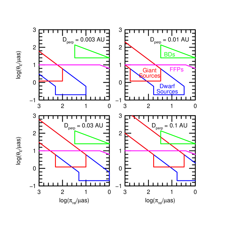
Figure 6: Sensitivity to microlens-parallax measurements of substellar objects (BDs and FFPs) as a function of Earth-satellite separation $D_{\perp}$, as specified in the four legends. Proposed experiments all have $D_{\perp}\sim 0.01\,{\rm au}$ (upper left panel). The BDs (green) and FFPs (magenta) are separated by the observed Einstein Desert. For $D_{\perp}\sim 0.01\,{\rm au}$, there is good sensitivity to FFPs, but essentially no sensitivity to BDs, which would require $D_{\perp}\gtrsim 0.3\,{\rm au}$.

Figure 6 compares these constraints to the expected locations of the two targeted populations, i.e., FFPs (magenta) and BDs (green), for four values of $D_{\perp}=(0.003,0.01,0.03,0.1)\,{\rm au}$. The axes ($\theta_{\rm E}$ versus $\pi_{\rm rel}$) are chosen to highlight what is known about these two populations, with the central fact being that the FFPs lie below the Einstein Desert ($\theta_{\rm E}\lesssim 10\,\mu{\rm as}$), whereas the BDs lie above it ($\theta_{\rm E}\gtrsim 25\,\mu{\rm as}$). As discussed by Gould et al. (2022), there are strong reasons for believing that the BDs are in the bulge, which we have represented by a cutoff at $\pi_{\rm rel}=0.03\,{\rm mas}$. We have also imposed a somewhat arbitrary mass limit on the FFPs of $M<5\,M_{\rm Jup}$ in order to illustrate that only if these objects are fairly massive can they actually be in the bulge. To illustrate the role of dwarf and giant sources, we choose $\theta_{*}=0.6\,\mu{\rm as}$ and $\theta_{*}=6\,\mu{\rm as}$, respectively.

Before discussing the implications of Figure 6, we note that the basic form of the allowed region is a band defined by a constant range of $\pi_{\rm E}$, i.e., $0.05<D_{\perp}\pi_{\rm E}/{\rm au}<1$, with a somewhat complex threshold at $\pi_{\rm rel}\gtrsim\theta_{*}$.

All current ideas for making these measurements are close to the top-right panel, i.e., the Earth-L2 distance. These include placing a satellite at L2 to continuously observe one KMT field (Gould et al., 2021; Ge et al., 2022), making observations from Earth of the Roman fields, observing the same fields simultaneously from Roman and Euclid, both in L2 halo orbits, or observing the same field from Roman in L2 and CSST in low-Earth orbit. The third would be intermediate between the top-left and top-right panels. See Gould et al. (2021). From Figure 6, these proposed experiments would be well-matched to measuring FFP masses for the known population, including members of both the disk and the bulge. However, these experiments will not measure masses for the known BD population. This would require $D_{\perp}\gtrsim 0.3\,{\rm au}$, i.e., more in the range of what is needed for BH mass measurements.

In summary, while some experiments proposed for the coming decade could lead to FFP mass measurements, there are no current prospects for BD mass measurements. Hence, $\theta_{\rm E}$-only surveys will remain the only method for detailed probing of this population for at least several decades.

7.3.2 Prospects for FSPL Measurements

Another possibility is that competing approaches might obtain a much larger number of FSPL measurements on one decade timescales compared to what can be achieved with current experiments. This would diminish, although it would not negate, the urgency of making such measurements based on current experiments.

The main competing approach would come from the Roman telescope, which is currently scheduled for launch in 2027 and would conduct a total of $\sim 1.2$ years of observations of $\sim 2\,{\rm deg}^{2}$ at a cadence of $\Gamma\sim 4\,{\rm hr}^{-1}$, using a broad $H$-band filter on a 2.4m telescope at L2.

Johnson et al. (2020) have comprehensively studied FFP detections by Roman, including detailed attention to finite-source effects, which yield FSPL events. They do not extend their mass range up to BDs, but it is not difficult to extrapolate from their maximum of $10^{3}\,M_{\oplus}$ to the BD range. However, our interest here is not so much the absolute number of such detections under various assumptions, but the relative number compared to current experiments.

In this section, we show that while Roman will greatly increase the number of FFP and isolated BD PSPL (i.e., $t_{\rm E}$-only) events relative to what can be achieved from the ground, it will not be competitive in identifying FSPL events (i.e., with $\theta_{\rm E}$ measurements), except in the regime $0.1\lesssim\theta_{\rm E}/\mu{\rm as}\lesssim 1$. We anticipate that the combination of the large space-based PSPL sample with the smaller ground-based FSPL sample will be more informative than either sample separately. However, we do not explore that aspect here because our primary concern is to investigate the uniqueness of the ground-based sample.

We begin by developing a new metric by which to compare the sensitivity of the KMT and Roman samples: S/N as a function rank ordered source luminosity. We focus on the KMT prime fields ($\sim 13\,{\rm deg}^{2}$), which have cadences similar to that of the Roman fields, i.e., $\Gamma=4\,{\rm hr}^{-1}$. We will show that about 11 times more microlensing events take place in these fields during 10 years of KMT observations than take place in the Roman fields during its observations. Here, we are not yet considering which of these events are actually detected by either project. Moreover, we are not yet restricting consideration to FSPL events.

In this context, if we wish to compare performance on an event-by-event basis, the events should first be rank-ordered by source luminosity (which is the most important factor in S/N). So, for example, we will show that KMT sources with $M_{I}=3.2$ should be compared to Roman sources with $M_{I}=6$, because there are the same number of microlensing events down to these two thresholds for the respective surveys.

Because the lens-source kinematics of the two experiments are essentially the same, the ratio of the number of events is given by the ratio of the products $\Omega\times\Delta t\times N_{S}\times N_{L}$, where

1. $\Omega$. Area of survey: $(13\,{\rm deg^{2}}/2\,{\rm deg}^{2}=6.5)$

2. $\Delta t$. Duration of survey: $(10\times 4\,{\rm months}/6\times 72\,{\rm days}=2.8)$

3. $N_{S}$. Surface density of sources: 1/1.29.

4. $N_{L}$. Surface density of lenses: 1/1.29.

That is, an overall ratio KMT:Roman of $6.5\times 2.8/1.29^{2}=11$. Here, we have adopted field sizes of $13\,{\rm deg}^{2}$ for the KMT prime fields versus $2\,{\rm deg}^{2}$ for Roman and durations of 4 months per year for 10 years for KMT versus six 72-day campaigns for Roman. In particular, we note that the KMT survey is nominally carried out for 8 months per year, but in the wings of the season, there are huge gaps due to the restricted times that the bulge can be observed. Moreover, KMT is affected by weather and other conditions (such as Moon) that restrict the period of useful observations. Thus, we consider that the effective observations are 4 months per year.

The mean latitude of the KMT prime fields is about $\langle|b|\rangle_{\rm KMT}\sim 2.35^{\circ}$, compared to $\langle|b|\rangle_{Roman}\sim 1.7^{\circ}$ for Roman. According to Nataf et al. (2013), this gives a factor of 1.29 advantage to Roman in bulge source density. For lenses that are in the bulge (as BDs are expected to mainly be), the advantage is identical. For disk lenses, it is roughly similar.

We use the HLF to calculate the cumulative distribution of sources. This distribution is given only for $M_{I}\leq 9$. However, we extend it to $M_{I}=12$ (i.e., to masses $M\sim 0.1\,M_{\odot}$) using the Chabrier (2005) mass function. We transform from mass to $I$-band luminosity using the $V$ and $K$ mass luminosity relations of Benedict et al. (2016) and the color-color relations of Bessell & Brett (1988). We refer to this combined luminosity function as the CHLF. We then adopt this as the unnormalized Roman distribution and multiply it by 11 to construct the KMT distribution before matching the two distributions. Figure 7 shows the result. As anticipated above, $M_{I}=6.00$ Roman sources are matched to $M_{I}=3.22$ KMT sources. Note that the viability of this approach depends on the fact that there are few useful sources outside the diagram. For Roman this is not an issue because the diagram goes almost to the bottom of the main sequence. If the matched KMT luminosity had been, say $M_{I,{\rm KMT}}=3.5$ at this point, then the diagram would be excluding many useful KMT sources. However, in fact, at the actual value ($M_{I}=6.0$) and for most applications, few such useful sources are being ignored. Nevertheless, these dim KMT sources can be important in some cases, so this must always be checked when applying this method of matched cumulative distributions.

We now evaluate the ratio between the Roman S/N and KMT S/N at each pair of matched values under the assumption that the source star is unblended and at various magnifications $A$. In each case, we assume that what is being measured is some small change in magnification $\Delta A$, so that the S/N ratios are

$$({\rm S/N})_{X}={f_{X}\Delta A\over\sqrt{f_{X}A+B_{X}}}$$ (13)

where the $f_{X}$ ($X=H$ or $X=I$) are the respective source flux of the matched sources, for Roman and KMT, and the $B_{X}$ are the respective backgrounds. Thus, their ratio,

$${({\rm S/N})_{H}\over({\rm S/N})_{I}}={f_{H}/f_{I}\over\sqrt{(f_{H}A+B_{H})/(f_{I}A+B_{I})}},$$ (14)

is independent of $\Delta A$. To make these evaluations, we adopt the following assumptions. Regarding KMT, we assume a zero point of 1 photon per (60 second) exposure at $I_{\rm zero}=28.0$ and with a background $I_{\rm back}=16.8$ as described above. Regarding Roman, we assume a zero point of 1 photon per (52 second) exposure at $H_{\rm zero}=30.4$ on the Vega system and a background of $H_{\rm back}=21.7$ per exposure. See Gould (2014). These backgrounds imply $B_{I}=3.02\times 10^{4}$ and $B_{H}=3.02\times 10^{3}$.

Next, we assume that the sources lie at $D_{S}=8\,{\rm kpc}$ and we adopt an $I$-band extinction $A_{I}=2$, corresponding to $A_{H}=0.23\,A_{I}=0.46$.

Finally, to convert from the $M_{I}$ (of the CHLF) to the required $M_{H}$ (needed to calculate the Roman source flux), we proceed as follows. For M dwarf sources ($M_{I}\geq 6.8$), we use the empirically calibrated mass-luminosity relations of Benedict et al. (2016) in $V$ and $K$, i.e., their Equation (10) and Table 12. We convert from $(V-K)$ to $(I-H)$ using the $VIHK$ relation of Bessell & Brett (1988) and then evaluate $M_{H}=M_{I}+(I-H)$. For the remainder of the CHLF, we use the following approximations $(I-H)=1.29-0.035\,M_{I}$, ($0\leq M_{I}<2$), $(I-H)=1.22-0.245\,(M_{I}-2)$, ($2\leq M_{I}<4$), $(I-H)=0.73\,M_{I}$, ($4\leq M_{I}<4.5$), and $(I-H)=0.73+0.402\,(M_{I}-4.5)$, ($4.5\leq M_{I}<6.8$).

The results are shown in Figure 8 for three case: $A=(1,10,100)$. The lower panel shows the S/N ratios as a function of $M_{I,Roman}$ so they can be referenced to Figure 7. However, the implications are best understood from the upper panel, which shows these ratios as a function of the cumulative distribution. The filled circles along the $(A=1)$ curve allow one to relate the two panels. These indicate (from right to left) $M_{I,Roman}=(12,11,10,\ldots)$. Figure 8 also has important implications for the Roman bound-planet“discovery space”. However, the main focus of the present work is on isolated substellar objects. Because these objects are themselves dark, and because they do not have a host, the assumption of “no blending” will usually be satisfied.

Figure 8 shows that over the entire CHLF and at all magnifications, Roman has higher S/N than KMT, implying that at each matched luminosity, Roman will detect at least as many PSPL isolated sub-stellar events as KMT. Hence, it will also detect at least as many from the CHLF as a whole. Because Roman S/N superiority is substantial, especially for $A=1$, over a substantial fraction of the CHLF, it may appear that it would detect many times more PSPL events. However, this proves to be the case only for low-mass FFPs, whereas the factor is more modest for isolated BDs.

The fundamental reason is that reliable detections can only be made up to some limit, e.g., $u_{0}<1$, regardless of S/N. For illustration, we assume that such a detection is possible for KMT assuming that the peak difference flux obeys $\Gamma u_{0}t_{\rm E}({\rm S/N})^{2}_{\rm peak}>\chi^{2}_{\rm min}=2000$. Because KMT is background-limited, this can be written $f_{I}>\sqrt{\chi^{2}_{\rm min}B_{I}/\Gamma u_{0}t_{\rm E}}/(A_{\rm max}-1)\rightarrow 2300(t_{\rm E}/{\rm day})^{-1/2}$. According to our assumption, $A_{I}=2$, this corresponds to $M_{I}<3.0+1.25\log(t_{\rm E}/{\rm day})$. Hence, adopting $\theta_{\rm E}=40\,\mu{\rm as}$ for a typical BD and assuming $\mu_{\rm rel}=6\,{\rm mas}\,{\rm yr}^{-1}$ (so, $t_{\rm E}=2.4\,$day), this implies $M_{I,{\rm KMT}}<3.5$, which matches to $M_{I,Roman}<6.8$ according to Figure 7. Carrying out a similar calculation for the Roman threshold, and noting that in the relevant range it is also background dominated, this yields $f_{H}>\sqrt{\chi^{2}_{\rm min}B_{H}/\Gamma u_{0}t_{\rm E}}/(A_{\rm max}-1)\rightarrow 735(t_{\rm E}/{\rm day})^{-1/2}$, i.e., $M_{H}<8.3+1.25\log(t_{\rm E}/{\rm day})$. Thus, for BDs, $M_{H}<8.8$, i.e., $M_{I}<11.1$. From Figure 7, Roman complete sensitivity to these BD PSPL events covers 4.7 times more of the cumulative fraction. Allowing for the gradual decline of $u_{0,{\rm max}}$ for KMT for dimmer sources, we can roughly estimate that Roman will detect 4 times more BD PSPL events, which is a relatively modest improvement.

By contrast, for FFPs with $\theta_{\rm E}=1\,\mu{\rm as}$, i.e., $t_{\rm E}=0.06\,$day, the corresponding limit for KMT would be $M_{I}<1.5$, for which $\theta_{*}\sim 3\,\mu{\rm as}$, i.e., $\rho\sim 3$. Hence, these would not be PSPL events, but rather FSPL. We will discuss these further below. On the other hand, for Roman, $M_{H}<6.8$, i.e., $M_{I}<8.7$ which covers about 1/4 of the cumulative fraction. Hence, Roman will be vastly more sensitive to PSPL FFPs at $\theta_{*}=1\,\mu{\rm as}$.

The method of matching cumulative source distributions cannot be used to compare Roman and KMT FSPL substellar events. First, the matched sources have different $\theta_{*}$, which is a fundamental parameter for FSPL events, Second, FSPL events are among the relatively rare class of applications for which “unmatched” KMT sources, i.e., $M_{I}>6.0$, play a crucial role.

Instead, we compare the returns of the two experiments by first setting a threshold $\Delta\chi^{2}=2000$ for each, which we approximate as $\Delta\chi^{2}=N_{\rm peak}[(A_{\rm max}-1)f_{X}]^{2}/(f_{X}+B_{X})$, where $A_{\rm max}=\sqrt{1+4/\rho^{2}}$ and $N_{\rm peak}=2\Gamma\theta_{*}/\mu_{\rm rel}\rightarrow 11.7(\theta_{*}/\mu{\rm as})$, and where we have made the evaluation by adopting $\mu_{\rm rel}=6\,{\rm mas}\,{\rm yr}^{-1}$. We further require $N_{\rm peak}\geq 3$ to ensure that the finite-source effects are adequately characterized. Finally, we demand $A_{\rm max}>1.06$, i.e., $\rho<5.7$ because of the difficulty of distinguishing lower-amplitude events from giant-source variability. While these prescriptions are simplified, they are adequate to characterize the relative sensitivity of the two experiments. For the source radii, we adopt $\theta_{*}=6\times 10^{-0.2\,M_{I}}\mu{\rm as}$, ($0\leq M_{I}<2$), $\theta_{*}=10^{0.378-0.3.01(M_{I}-2)}\mu{\rm as}$, ($2\leq M_{I}<4$), $\theta_{*}=(R_{\odot}/D_{S})\times 10^{-0.2\,(M_{I}-4.07)}$, ($4\leq M_{I}<4.5$), $\theta_{*}=10^{-0.320-0.041(M_{I}-4.5)}\mu{\rm as}$, ($4.5\leq M_{I}<6.8$), and $\theta_{*}=(M/M_{\odot})(R_{\odot}/D_{S})$, ($M_{I}>6.8$), where $D_{S}=8\,{\rm kpc}$.

The results are shown in Figure 9. There is a rapid transition at $\theta_{\rm E}\sim 1\,\mu{\rm as}$: below this threshold, KMT loses all sensitivity, while Roman retains constant sensitivity for almost a decade; above the threshold, KMT completely dominates the detections, reaching a factor 11 in the BD regime, $\theta_{*}\gtrsim 30\,\mu{\rm as}$. The physical reason for this dominance is simple. At the adopted threshold of detectability, $\theta_{*,\rm thresh}=(3/2)\mu_{\rm rel}/\Gamma=0.256\,\mu{\rm as}$, i.e., $M_{I,\rm thresh}=8.25$ or $I_{S}=24.75$, the source is magnified by $A_{\rm max}=2/\rho\rightarrow 230$ to $I\sim 18.8$, which creates a marginally detectable event. Thus, all sources (down to this threshold) yield detectable events from either KMT or Roman, but because the former has 11 times more events, it has 11 times more detections. In fact, the completeness analysis of Section 7.1 shows that only of order half of such high-magnification events from uncataloged sources are recovered by current KMT searches. This could be rectified by additional specialized searches for such “spike events” but even without such an effort, KMT will still dominate in this regime.

By the same token, at $\theta_{\rm E}=1\,\mu{\rm as}$, faint sources are insufficiently magnified to boost them to detectability. For example, for near-optimal sources, $\theta_{*}=\theta_{\rm E}$, i.e., $M_{I}=3.28$ or $I_{S}=19.78$ and with peak magnification $A_{\rm max}=\sqrt{5}$, the difference magnitude is only $I_{\rm diff}=19.55$. However, based on its far greater flux counts and lower background, such events are easily detected by Roman.

We emphasize that the “flat” form of the Roman curve over 3 decades does not mean that one expects equal numbers of detections across this range: based on what we know today (Gould et al., 2022), there could be of order 40 times more FFPs at $\theta_{*}=10^{-0.8}\mu{\rm as}$ compared to $\theta_{*}=10^{+0.8}\mu{\rm as}$.

7.3.3 Summary

The only way to press forward the study of isolated bulge BDs is by FSPL events from ground-based surveys, mainly KMT. It is not possible to obtain a substantial number of full mass-distance measurements for these objects from any current, planned, or proposed experiments. Regarding FSPL BD events, there are no other current or currently planned experiments that could compete with KMT.

The situation is more nuanced for FFPs. First, in the next decade, new experiments could yield mass-distance measurements, assuming that the current proposals for these are approved and implemented. Second, Roman will be increasingly competitive for FFPs within the range $2\gtrsim\theta_{\rm E}/\mu{\rm as}\gtrsim 1$ and will be completely dominant for $\theta_{\rm E}\lesssim 1\,\mu{\rm as}$.

7.4 Comments on the Recent MOA FSPL Search

As the present paper was being completed, Koshimoto et al. (2023) reported results from a comprehensive search for FSPL events in Microlensing Observations in Astrophysics (MOA) Collaboration data over the 9 years from 2006 to 2014. Here we comment on a few implications that relate to results and ideas that we have presented.

The most important point is that Koshimoto et al. (2023) searched for FSPL events with both giant and dwarf sources, which is what we have broadly advocated here. In particular, the inclusion of “dwarf” (including main-sequence and subgiant) sources led to the discovery of a very small FFP, MOA-9yr-5919, with $\theta_{\rm E}=0.90\pm 0.14\,\mu{\rm as}$. Being the second such discovery (after OGLE-2016-BLG-1928, $\theta_{\rm E}=0.84\pm 0.06\,\mu{\rm as}$, Mróz et al. 2020b), it strongly implies that such objects are very common. That is, a single such discovery would be consistent with a low-probability, e.g., $p=5\%$, detection from a relatively rare population. However, two such chance discoveries would occur only at ${\cal O}(p^{2})$. It was exactly this logic that led Gould et al. (2006) to conclude that “Cool Neptune-like Planets are Common” based on two detections, which was soon confirmed by Sumi et al. (2010) and then, subsequently, by of order two dozen other detections (Suzuki et al. 2016, Zang et al., in prep). The inclusion of dwarf sources was crucial to this discovery: if the same planet had transited a typical source from the Gould et al. (2022) giant-star survey, with $\theta_{*}\sim 6\,\mu{\rm as}$, it would have had $\rho\sim 6.7$ and hence excess magnification $A-1\simeq 2/\rho^{2}\sim 4.5\%$ and would not have been detected.

Sumi et al. (2023) show (their Table 3), that the MOA and KMT surveys are consistent in their constraints on the FFP population, including both the power-law index and its normalization $Z$. In particular, at the same zero-point, they find $Z=0.53^{+0.19}_{-0.40}$ versus $0.39\pm 0.20$ FFPs per dex per (stars + BDs) for KMT.

At first sight, one may wonder about the consistency of the detection rates of the KMT giant-source survey, which discovered 29 FSPL events satisfying $I_{0}<16.5$, with the “giant component” of the MOA survey, with 7 such events. However, we now show that the ratio of detections is consistent with expectations. First, Koshimoto et al. (2023) note that they are insensitive to the biggest $(\theta_{*}\gtrsim 10\,\mu{\rm as})$ sources from the KMT survey due to saturation. (For many of these bright sources, KMT recovered from saturation using $V$-band observations.)  From Figure 2 of Sumi et al. (2023), such a cut would eliminate $\sim 1/3$ of KMT events. Second, the MOA detector is about half the size of the KMT detectors (2.2 versus 4 square degrees), and in line with this fact, it surveys roughly half the area (i.e., mainly southern bulge versus full bulge). Third, the KMT survey employs three telescopes, whereas the MOA survey uses one. Moreover, while MOA and KMTA have comparable conditions, KMTS and KMTC have better conditions. If we were considering very short events, which are mainly localized to a single observatory, then this would give KMT a 4:1 advantage. However, because giant-source events are very long, often covering two or more observatories, we reduce this estimate to 3:1. Finally, the MOA survey covered 9 years while the KMT covered 4 years. Combining all factors, we expect a ratio of MOA-to-KMT giant-source FSPL events of $(2/3)\times(1/2)\times(1/3)\times(9/4)=25\%$ compared to an observed ratio of 24%, which is consistent.

Table 1: KMT-2022-BLG-2397 Light Curve Parameters

Parameter	Units	Value	Error
$t_{0}$	(HJD′)	9812.31849	0.00035
$t_{\rm E}$	(day)	1.35	0.11
$t_{\rm eff}$	(day)	0.03588	0.00087
$t_{*}$	(day)	0.05016	0.00065
$f_{S}t_{\rm E}$	(day)	0.1047	0.0025
$u_{0}$		0.0266	0.0025
$\rho$		0.0371	0.0032
$I_{\rm S,KMTC03}$		20.78	0.11
$z_{0}$		0.715	0.017

Note. — $t_{\rm eff}$, $t_{*}$, $f_{S}t_{\rm E}$, and $z_{0}$ are derived parameters and are not fit separately.

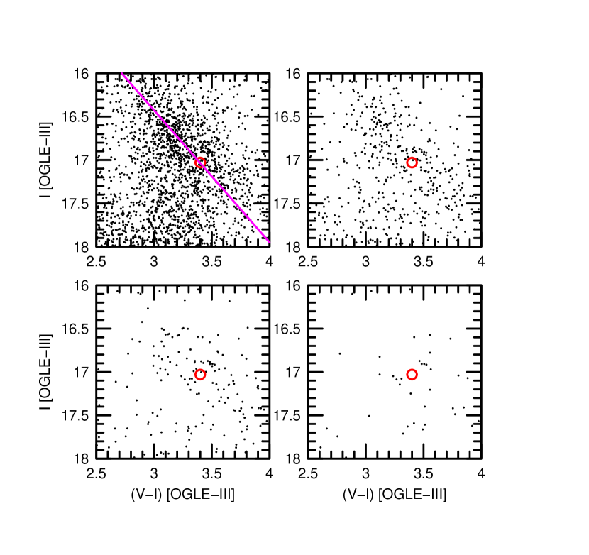
Figure 2: Four views of the CMD in the region near the red clump for KMT-2022-BLG-2397, including stars within radii of $200^{\prime\prime}$ (upper left), $100^{\prime\prime}$ (upper right), $60^{\prime\prime}$ (lower left), and $30^{\prime\prime}$ (lower right) from the event. The red circle represents the adopted centroid of the red clump at the location of the source star. The magenta line is the reddening direction, as derived from the extension of the clump in the $200^{\prime\prime}$ panel.

Figure 7: Matched cumulative distributions of microlensing events taking place within the purview of the 10-year KMT survey and the 5-year Roman survey, according to the $I$-band luminosities of each event. Because 11 times more microlensing events take place (not necessarily detected) for KMT, relatively brighter KMT sources are matched one-for-one to relatively fainter Roman sources. As shown by Figure 8, this effect tends to mitigate the otherwise overwhelming advantage of Roman’s higher throughput, lower extinction, and lower background.

Figure 8: Ratios of S/N of matched events (see Figure 7) of Roman relative to KMT for three different magnifications, $A=(1,10,100)$. The lower panel shows these as a function of the $M_{I,Roman}$ parameter in order to make contact with Figure 7. Note, however, that this is a label used for matching: the Roman S/N is calculated in $H$-band. The upper panel shows the same ratios as a function of the cumulative distribution of sources, so that the occurrence of microlensing events (not necessarily their detection) is uniformly distributed along the abscissa. At moderate to high magnifications, which account for most ground-based planets, Roman has an advantage of a factor 2–4, whereas at low magnifications, Roman has an overwhelming advantage over most of this range. Filled circles show (right to left) $M_{I,Roman}=(12,11,\ldots)$.

References

- Alard & Lupton (1998) Alard, C. & Lupton, R.H.,1998, ApJ, 503, 325
- Albrow (2017) Albrow, M.D. Michaeldalbrow/Pydia: InitialRelease On Github., vv1.0.0, Zenodo
- Albrow et al. (2009) Albrow, M. D., Horne, K., Bramich, D. M., et al. 2009, MNRAS, 397, 2099
- Benedict et al. (2016) Benedict, G.F., Henry, T.J., Franz, O.G., et al. 2016, AJ, 152, 141
- Bennett & Rhie (2002) Bennett, D.P., & Rhie, S.H. 2002, ApJ, 579, 638
- Bennett et al. (2012) Bennett, D.P., Sumi, T., Bond, I.A., et al. 2012, ApJ, 757, 119
- Bensby et al. (2013) Bensby, T. Yee, J.C., Feltzing, S. et al. 2013, A&A, 549, A147
- Bessell & Brett (1988) Bessell, M.S., & Brett, J.M. 1988, PASP, 100, 1134
- Cassan et al. (2021) Cassan, A., Ranc, C., Abel, O., et al., 2021, Nature Astronomy, 6, 121
- Chabrier (2005) Chabrier, G. 2005, Astrophysics and Space Science Library, 327, 41
- Chung et al. (2017) Chung, S.-J., Zhu, W., Udalski, A., 2017, ApJ, 838, 154
- Delplancke et al. (2001) Delplancke, F., Górski, K.M., & Richichi, A. 2001, A&A, 375, 701
- Dong et al. (2019) Dong, S., Mérand, A., Delplancke-Strobale, F. 2019, ApJ, 871, 70
- Gaia Collaboration et al. (2016) Gaia Collaboration, Prusti, T., de Bruijne, J.H.J., et al. 2016, A&A, 595, A1
- Gaia Collaboration et al. (2018) Gaia Collaboration, Brown, A. G. A., Vallenari, A., et al. 2018, A&A, 616, 1
- Ge et al. (2022) Ge, J., Zhang, H., Zang, W., et al. 2022, arXiv:2206.06693
- Ghosh et al. (2004) Ghosh, H., DePoy, D.L., Gal-Yam, A., et al. 2004, ApJ, 615, 450
- Gould (1992) Gould, A. 1992, ApJ, 392, 442
- Gould (1994a) Gould, A. 1994a, ApJ, 421, L71
- Gould (1994b) Gould, A. 1994b, ApJ, 421, L75
- Gould (1997) Gould, A. 1997, ApJ, 480, 188
- Gould (2014) Gould, A. 2014, JKAS, 47, 279
- Gould (2022) Gould, A. 2022, arXiv:2209.12501
- Gould et al. (1994) Gould, A., Miralda-Escudé, J. & Bahcall, J.N. 1994, ApJ, 423, L105
- Gould et al. (2006) Gould, A., Udalski, A., An, D. et al. 2006, ApJ, 644, L37
- Gould et al. (2009) Gould, A., Udalski, A., Monard, B. et al. 2009, ApJ, 698, L147
- Gould et al. (2010) Gould, A., Dong, S., Gaudi, B.S. et al. 2010, ApJ, 720, 1073
- Gould & Yee (2013) Gould, A. & Yee, Y.C. 2013, ApJ, 764, 107
- Gould & Yee (2014) Gould, A. & Yee, Y.C. 2013, ApJ, 784, 64
- Gould et al. (2021) Gould, A., Zang, W., Mao, S., & Dong, S., 2021, RAA, 21, 133
- Gould et al. (2022) Gould, A., Jung, Y.K., Hwang, K.-H. et. al., 2022, JKAS, 55, 173
- Griest & Safizadeh (1998) Griest, K. & Safizadeh, N. 1998, ApJ, 500, 37
- Han et al. (2020) Han, C., Lee, C.-U., et al. 2020, AJ, 159, 134
- Hawking (1975) Hawking, S.W. 1975, Communications of Mathematical Physics, 43, 199
- Henderson et al. (2014) Henderson, C.B., Gaudi, B.S., Han, C., et al. 2014, ApJ, 794, 52
- Hog et al. (1995) Hog, E., Novikov, I.D., & Polanarev, A.G. 1995, A&A, 294, 287
- Holtzman et al. (1998) Holtzman, J.A., Watson, A.M., Baum, W.A., et al. 1998, AJ, 115, 1946
- Holz & Wald (1996) Holz, D.E. & Wald, R.M. 1996, ApJ471, 64
- Johnson et al. (2020) Johnson, S.A., Penny, M., Gaudi, B.S., et al. 2020, AJ, 160, 123
- Jung et al. (2023) Jung, Y.K., Zang, W., Wang, H., et al. 2023, AJ, 165, 226
- Kervella et al. (2004) Kervella, P., Bersier, D., Mourard, D., et al. 2004, A&A, 428, 587
- Kim et al. (2016) Kim, S.-L., Lee, C.-U., Park, B.-G., et al. 2016, JKAS, 49, 37
- Kim et al. (2018a) Kim, D.-J., Kim, H.-W., Hwang, K.-H., et al., 2018a, AJ, 155, 76
- Kim et al. (2018b) Kim, H.-W., Hwang, K.-H., Shvartzvald, Y., et al. 2018b, arXiv:1806.07545
- Kim et al. (2021) Kim, H.-W., Hwang, K.-H., Gould, A., et al. 2021, AJ, 162, 15
- Koshimoto et al. (2023) Koshimoto, N., Sumi, T., Bennett, D.P., et al. 2023, arXiv:2303.08279
- Kondo et al. (2019) Kondo, I., Sumi, T., Bennett, D.P., et al. 2019, AJ, 158, 224
- Lam et al. (2020) Lam, C.Y., Lu, J.R., Hosek, M.W. Jr., Dawson, W.A., & Golovich, N.R., 2020, ApJ, 889, 31
- Lam et al. (2022) Lam, C.Y., Lu, J.R., Udalski, A., et al., 2022, ApJ, 933, L23
- Miyamoto & Yoshii (1995) Miyamoto, M. & Yoshii, Y. 1995, AJ, 110, 1427
- Mróz et al. (2017) Mróz, P., Udalski, A., Skowron, J., et al. 2017, Nature, 548, 183
- Mróz et al. (2018) Mróz, P., Ryu, Y.-H., Skowron, J., et al. 2018, AJ, 155, 121
- Mróz et al. (2019) Mróz, P., Udalski, A., Bennett, D.P., et al. 2019, A&A, 622, A201
- Mróz et al. (2020a) Mróz, P., Poleski, R., Han, C., et al. 2020a, AJ, 159, 262
- Mróz et al. (2020b) Mróz, P., Poleski, R., Gould, A., et al. 2020b, ApJ, 903, 11
- Mróz et al. (2022) Mróz, P, Udalski, A., & Gould, A., 2022, ApJ, 937, L24
- Nataf et al. (2013) Nataf, D.M., Gould, A., Fouqué, P. et al. 2013, ApJ, 769, 88
- Nemiroff & Wickramasinghe (1994) Nemiroff, R.J., & Wickramasinghe, W.A.D.T. 1994, ApJ, 424, L21
- Refsdal (1966) Refsdal, S. 1966, MNRAS, 134, 315
- Sahu et al. (2022) Sahu, K.C., Anderson, J., Casertano, S., st al. 2022, ApJ, 933, 83
- Shan et al. (2021) Shan, Y., Yee, J.C., Bailey, V. et al. 20121 ApJ, 908, 240
- Shin et al. (2018) Shin, I.-G., Yee, J.C., Skowron, J. et al. 2018, ApJ, 863, 23
- Shvartzvald et al. (2019) Shvartzvald, Y., Yee, J.C., Skowron, J. et al. 2019, AJ, 157, 106
- Shvartzvald et al. (2023) Shvartzvald, Y., Waxman, E., Gal-Yam, A. et al. 2023, arXiv:2304.14482
- Sumi et al. (2010) Sumi, T., Bennett, D.P., Bond, I.A., et al. 2010, ApJ, 710, 1641
- Sumi et al. (2011) Sumi, T., Kamiya, K., Bennett, D. P., et al. 2011, Nature, 473, 349
- Sumi et al. (2023) Sumi, T., Koshimoto, N., Bennett, D.P., et al. 2023, arXiv:2303.08280
- Suzuki et al. (2016) Suzuki, D., Bennett, D.P., Sumi, T., et al. 2016, ApJ, 833, 145
- Szymański et al. (2011) Szymański, M.K., Udalski, A., Soszyński, I., et al. 2011, Acta Astron., 61, 83
- Tomaney & Crotts (1996) Tomaney, A.B. & Crotts, A.P.S. 1996, au, 112, 2872
- Walker (1995) Walker, M.A. 1995, ApJ, 453, 37
- Witt & Mao (1994) Witt, H.J., & Mao, S. 1994, ApJ, 429, 66
- Yee et al. (2021) Yee, J.C., Zang, W., Udalski, A. et al. 2021, AJ, 162, 180
- Yoo et al. (2004) Yoo, J., DePoy, D.L., Gal-Yam, A. et al. 2004, ApJ, 603, 139
- Zang et al. (2020) Zang, W., Dong, S., Gould, A., et al. 2020, ApJ, 897, 180
- Zang et al. (2021) Zang, W., Hwang, K.-H., Udalski, A., et al. 2021, AJ, 162, 163
- Zhu et al. (2016) Zhu, W., Calchi Novati, S., Gould, A., et al. 2016, ApJ, 825, 60