Form factors of $\Omega^{-}$ in a covariant quark-diquark approach

Abstract

The electromagnetic and gravitational form factors of $\Omega^{-}$, a spin-3/2 hyperon composed of three $s$ quarks, are calculated by using a covariant quark-diquark approach. The model parameters are determined by fitting to the form factors of the lattice QCD calculations. Our obtained electromagnetic radii, magnetic moment, and electric-quadrupole moment are in agreement with the experimental measurements and some other model calculations. Furthermore, the mass and spin distributions of $\Omega^{-}$ from the gravitational form factors are also displayed. It is found that the mass radius is smaller than its electromagnetic ones. Finally, the interpretations of the energy density and momentum current distribution are also discussed.

1 Introduction

Form factors (FFs), such as electromagnetic form factors (EMFFs) and gravitational form factors (GFFs), are the very important physical quantities that describe the internal structure of a hadron. They carry the fundamental and essential information, such as the distributions of the electric charge, magnetic moment, mass and spin. There have been many studies of EMFFs [1, 2, 3, 4, 5, 6] and GFFs [7, 8, 9, 10, 11]. In particular much work has been devoted to study the properties of the various low-spin hadrons, such as spin-0 ($\pi$ [12, 13, 8]), spin-1/2 (nucleon [14, 15, 16, 17]), and spin-1 ($\rho$ [18] and deuteron [19, 20, 21, 22]). Experimentally, EMFFs can be detected from the processes driven by the electromagnetic interactions. The corresponding processes, such as the hadron production processes from $e^{+}e^{-}$ annihilation [23, 24, 25] and the inverse processes [26], are accessible. However, the direct detection of GFFs is not realistic due to the weak gravitational interaction. Fortunately, they can be obtained via the generalized parton distributions (GPDs) [27, 28, 29, 30, 31], and GPDs can be extracted from deeply virtual Compton scattering (DVCS) by using sum rules, from vector-meson electro-production processes, and from generalized distribution amplitudes (GDAs) [8].

As the total spin of the system increases, there are more FFs, such as electric-quadrupole, magnetic-octupole, energy-quadrupole, and angular momentum-octupole form factors for a spin-3/2 particle. Although some of the spin-3/2 particles have been discussed and studied [32, 33, 34, 35, 36, 37, 38], their detailed information is still lacking compared to those of the low-spin particles. $\Delta$ resonance is the typical spin-3/2 particle which has been usually considered [39, 40, 38, 41]. Another typical spin-3/2 particle is $\Omega^{-}$ [39, 25, 42]. However, most of the work, in the literature, only focus on its EMFFs.

Comparing the $\Omega^{-}$ hyperon with the $\Delta$ resonance, we see that the former has a longer lifetime $(c\tau=2.461\leavevmode\nobreak\ \text{cm})$ and it undergoes weak decays. Therefore, we expect that $\Omega^{-}$ is more realistic to be measured. On the one hand, the $\Omega^{-}$ form factors in the time-like region have been measured by the $e^{+}e^{-}\rightarrow\Omega^{-}\bar{\Omega}^{+}$ at CLEO [25]. Based on the $e^{+}e^{-}\rightarrow B\bar{B}$ process, the facilities, such as BABAR [43, 44], BES III [45, 46, 47], CLEO [48], and PANDA [49], all have the chance to measure its structures by producing the secondary $\Omega^{-}$ beam. In addition, $\Omega^{-}$ event can also be produced in the inclusive reaction $p+Be\rightarrow\Omega+X$ [50]. On the other hand, the more promising and reliable method to describe the FFs of $\Omega^{-}$ is the Lattice QCD (LQCD). Except for some LQCD calculations [51, 52, 53], there are also some model calculations of FFs, such as the chiral constituent quark model ($\chi$CQM) [54, 55, 56], the chiral perturbation theory ($\chi$PT) [57, 58], the $1/N_{c}$ expansion [59, 60], the SU(2) Skyme model [61], the bag model [62], the QCD sum rule (QCDSR) [33, 63], the relativistic quark model (RQM) [32, 64], the non-relativistic quark model (NRQM) [65, 66], and so on.

In this work, we give a study of the electromagnetic properties of $\Omega^{-}$ and its mechanical properties. It should be remained that prior to this work, we have carried out the calculations and analyses for the FFs of the $\Delta$ resonance and for its generalized parton distributions in a covariant quark-diquark approach [67, 68, 69]. Here the same approach is employed to study the FFs of the $\Omega^{-}$ hyperon [5, 67]. We know that $\Omega^{-}$ is composed of three $s$ quarks and it is convenient to consider the two $s$ quarks as a whole, i.e. as an axial-vector diquark. Thus, we may deal with an effective two-body system without losing the main internal structure information, and consequently, the final FFs can be obtained by summing the contributions of the quark and diquark. It should be addressed that the diquark structure can be explicitly considered by replacing the quark electromagnetic and energy momentum tensor (EMT) currents by the corresponding ones of the diquark.

This paper is organized as follows. In Sec. 2, FFs and the quark-diquark approach are briefly discussed. Our numerical results of EMFFs in comparison with the results of LQCD and our GFFs are given in Sec. 3, where our obtained energy and angular momentum distributions and their representations in the coordinate space are also displayed. In addition, the quantities related to the ”$D$-term”, pressures, and shear forces are discussed as well. Finally, section 4 is devoted to a summary.

2 Form factors and quark-diquark approach

2.1 Form factors of the spin-3/2 system

In this work, the same approach as Ref. [67] is employed to study the FFs of the $\Omega^{-}$ hyperon. For a spin-3/2 particle, the matrix element of the electromagnetic current can be written, in terms of the form factors $F_{i,j}^{V,a}$ as [70]

$$\begin{split}\left\langle p^{\prime},\lambda^{\prime}\left|\hat{J}_{a}^{\mu}\left(0\right)\right|p,\lambda\right\rangle=&-\bar{u}_{\alpha^{\prime}}\left(p^{\prime},\lambda^{\prime}\right)\biggl{[}\frac{P^{\mu}}{M}\left(g^{\alpha^{\prime}\alpha}F_{1,0}^{V,a}\left(t\right)-\frac{q^{\alpha^{\prime}}q^{\alpha}}{2M^{2}}F_{1,1}^{V,a}\left(t\right)\right)\\ &+\frac{i\sigma^{\mu\nu}q_{\nu}}{2M}\left(g^{\alpha^{\prime}\alpha}F_{2,0}^{V,a}\left(t\right)-\frac{q^{\alpha^{\prime}}q^{\alpha}}{2M^{2}}F_{2,1}^{V,a}\left(t\right)\right)\biggr{]}u_{\alpha}\left(p,\lambda\right),\end{split}$$ (1)

where $u_{\alpha}\left(p,\lambda\right)$ is the Rarita-Schwinger spinor and the normalization is taken to be $\bar{u}_{\sigma^{\prime}}(p)u_{\sigma}(p)=-2M\delta_{\sigma^{\prime}\sigma}$ with $M$ being the $\Omega^{-}$ mass. In Eq. (1) the kinematical variables $P^{\mu}=(p^{\mu}+p^{\prime\mu})/2$, $q^{\mu}=p^{\prime\mu}-p^{\mu}$, and $t=q^{2}$ are employed and $p\,(p^{\prime})$ is the momentum of the initial (final) state. Moreover, the form factors $F_{i,j}^{V,a}$ are defined flavor by flavor and include the contribution of gluon in general. The total form factors $F_{i,j}^{V}=\underset{a}{\sum}F_{i,j}^{V,a}$ are obtained as the index $a$ runs from the quark to gluon. Here, since we only consider the constituent quark, the gluon contribution is simply and effectively included.

In our numerical calculation, the average of the initial and final momenta is defined as $P^{\mu}=(E,\bm{0})$ and the momentum transfer is $q^{\mu}=(0,\bm{q})$ by using the Breit frame. Thus, $t=q^{2}=-\bm{q}^{2}=4(M^{2}-E^{2})$. The EMFFs of the spin-3/2 particle can be further expressed in terms of the electromagnetic covariant vertex function coefficients $F_{i,j}^{V}$, where $i=1,2$ and $j=0,1$, as [71]

$$G_{E0}\left(t\right)= \left(1+\frac{2}{3}\tau\right)[F_{2,0}^{V}(t)+(1+\tau)(F_{1,0}^{V}(t)-F_{2,0}^{V}(t))]+\frac{2}{3}\tau(1+\tau)[F_{2,1}^{V}(t)+(1+\tau)(F_{1,1}^{V}(t)-F_{2,1}^{V}(t))],$$ (a)

$$G_{E2}\left(t\right)= [F_{2,0}^{V}(t)+(1+\tau)(F_{1,0}^{V}(t)-F_{2,0}^{V}(t))]+(1+\tau)[F_{2,1}^{V}(t)+(1+\tau)(F_{1,1}^{V}(t)-F_{2,1}^{V}(t))],$$ (b)

$$G_{M1}\left(t\right)= \left(1+\frac{4}{5}\tau\right)F_{2,0}^{V}\left(t\right)+\frac{4}{5}\tau(\tau+1)F_{2,1}^{V}\left(t\right),$$ (c)

$$G_{M3}\left(t\right)= F_{2,0}^{V}\left(t\right)+(\tau+1)F_{2,1}^{V}\left(t\right),$$ (d)

where $\tau=-t/(4M^{2})$ and $G_{E0}$, $G_{E2}$, $G_{M1}$, and $G_{M3}$ represent the electric-monopole, electric-quadrupole, magnetic-dipole, and magnetic-octupole form factors, respectively. The intrinsic electromagnetic properties, including the electric charge, magnetic moment, electric-quadrupole moment, and magnetic-octupole moment, are obtained in the forward limit, $t=0$. The electric-monopole and magnetic-dipole form factors give the corresponding electric charge and magnetic radii of the particle as [51]

$$\left\langle r^{2}\right\rangle_{E0}=\frac{6}{G_{E0}(0)}\frac{d}{dt}G_{E0}(t)\Big{|}_{t=0},\quad\left\langle r^{2}\right\rangle_{M1}=\frac{6}{G_{M1}(0)}\frac{d}{dt}G_{M1}(t)\Big{|}_{t=0}.$$ (3)

Similarly to EMFFs, the matrix element of the EMT current can be written as [38]

$$\begin{split}&\left\langle p^{\prime},\lambda^{\prime}\left|\hat{T}^{\mu\nu}_{a}(0)\right|p,\lambda\right\rangle\\ &\leavevmode\nobreak\ \leavevmode\nobreak\ \leavevmode\nobreak\ =-\bar{u}_{\alpha^{\prime}}\left(p^{\prime},\lambda^{\prime}\right)\bigg{[}\frac{P^{\mu}P^{\nu}}{M}\left(g^{\alpha^{\prime}\alpha}F_{1,0}^{T,a}(t)-\frac{q^{\alpha^{\prime}}q^{\alpha}}{2M^{2}}F_{1,1}^{T,a}(t)\right)+\frac{\left({q}^{\mu}{q}^{\nu}-{g}^{\mu\nu}q^{2}\right)}{4M}\left({g}^{\alpha^{\prime}\alpha}F_{2,0}^{T,a}(t)-\frac{{q}^{\alpha^{\prime}}{q}^{\alpha}}{2M^{2}}F_{2,1}^{T,a}(t)\right)\\ &\leavevmode\nobreak\ \leavevmode\nobreak\ \leavevmode\nobreak\ \leavevmode\nobreak\ \leavevmode\nobreak\ +Mg^{\mu\nu}\left(g^{\alpha^{\prime}\alpha}F_{3,0}^{T,a}(t)-\frac{q^{\alpha^{\prime}}q^{\alpha}}{2M^{2}}F_{3,1}^{T,a}(t)\right)+\frac{i{P}^{\{\mu}\sigma^{\nu\}\rho}q_{\rho}}{2M}\left(g^{\alpha^{\prime}\alpha}F_{4,0}^{T,a}(t)-\frac{q^{\alpha^{\prime}}q^{\alpha}}{2M^{2}}F_{4,1}^{T,a}(t)\right)\\ &\leavevmode\nobreak\ \leavevmode\nobreak\ \leavevmode\nobreak\ \leavevmode\nobreak\ \leavevmode\nobreak\ -\frac{1}{M}\left({q}^{\{\mu}g^{\nu\}\{\alpha^{\prime}}{q}^{\alpha\}}-2q^{\alpha^{\prime}}q^{\alpha}g^{\mu\nu}-g^{\alpha^{\prime}\{\mu}g^{\nu\}\alpha}q^{2}\right)F_{5,0}^{T,a}(t)+Mg^{\alpha^{\prime}\{\mu}g^{\nu\}\alpha}F_{6,0}^{T,a}(t)\bigg{]}u_{\alpha}\left(p,\lambda\right),\end{split}$$ (4)

where $F^{T}_{i,j}=\underset{a}{\sum}F_{i,j}^{T,a}$ stand for the GFFs of the spin-3/2 hadron and the conventions $a^{\{\mu}b^{\nu\}}=a^{\mu}b^{\nu}+a^{\nu}b^{\mu}$ and $a^{[\mu}b^{\nu]}=a^{\mu}b^{\nu}-a^{\nu}b^{\mu}$ are adopted. In the Breit frame, the gravitational multipole form factors (GMFFs) of the spin-3/2 particle can be expressed in terms of its GFFs $F^{T}_{i,j}$ as [38]

$${\varepsilon}_{0}\left(t\right) =F^{T}_{1,0}(t)+\frac{t}{6M^{2}}\biggl{[}-\frac{5}{2}F^{T}_{1,0}(t)-F^{T}_{1,1}(t)-\frac{3}{2}F^{T}_{2,0}(t)+4F^{T}_{5,0}(t)+3F^{T}_{4,0}\biggr{]}$$

$$+\frac{t^{2}}{12M^{4}}\biggl{[}\frac{1}{2}F^{T}_{1,0}(t)+F^{T}_{1,1}(t)+\frac{1}{2}F^{T}_{2,0}(t)+\frac{1}{2}F^{T}_{2,1}(t)-4F^{T}_{5,0}(t)-F^{T}_{4,0}(t)-F^{T}_{4,1}(t)\biggr{]}$$

$$+\frac{t^{3}}{48M^{6}}\biggl{[}-\frac{1}{2}F^{T}_{1,1}(t)-\frac{1}{2}F^{T}_{2,1}(t)+F^{T}_{4,1}(t)\biggr{]},$$ (a)

$${\varepsilon}_{2}(t) =-\frac{1}{6}\biggl{[}F^{T}_{1,0}(t)+F^{T}_{1,1}(t)-4F^{T}_{5,0}(t)\biggr{]}$$

$$+\frac{t}{12M^{2}}\biggl{[}\frac{1}{2}F^{T}_{1,0}(t)+F^{T}_{1,1}(t)+\frac{1}{2}F^{T}_{2,0}(t)+\frac{1}{2}F^{T}_{2,1}(t)-4F^{T}_{5,0}(t)-F^{T}_{4,0}-F^{T}_{4,1}(t)\biggr{]}$$

$$+\frac{t^{2}}{48M^{4}}\biggl{[}-\frac{1}{2}F^{T}_{1,1}(t)-\frac{1}{2}F^{T}_{2,1}(t)+F^{T}_{4,1}(t)\biggr{]},$$ (b)

$$\mathcal{J}_{1}(t) =F^{T}_{4,0}(t)-\frac{t}{5M^{2}}\biggl{[}F^{T}_{4,0}(t)+F^{T}_{4,1}(t)+5F^{T}_{5,0}(t)\biggr{]}+\frac{t^{2}}{20M^{4}}F^{T}_{4,1}(t),$$ (c)

$$\mathcal{J}_{3}(t) =-\frac{1}{6}\biggl{[}F^{T}_{4,0}(t)+F^{T}_{4,1}(t)\biggr{]}+\frac{t}{24M^{2}}F^{T}_{4,1}(t),$$ (d)

$$D_{0}(t) =F^{T}_{2,0}(t)-\frac{16}{3}F^{T}_{5,0}(t)-\frac{t}{6M^{2}}\bigg{[}F^{T}_{2,0}(t)+F^{T}_{2,1}(t)-4F^{T}_{5,0}(t)\bigg{]}+\frac{t^{2}}{24M^{4}}F^{T}_{2,1}(t),$$ (e)

$$D_{2}(t) =\frac{4}{3}F^{T}_{5,0}(t),$$ (f)

$$D_{3}(t) =\frac{1}{6}\bigg{[}-F^{T}_{2,0}(t)-F^{T}_{2,1}(t)+4F^{T}_{5,0}(t)\bigg{]}+\frac{t}{24M^{2}}F^{T}_{2,1}(t),$$ (g)

where the non-conserving terms, $F^{T}_{3,0(1)}$ and $F^{T}_{6,0}$ are simply ignored because they should vanish if we add the gluon contributions explicitly. In Eq. (5), ${\varepsilon}_{0(2)}$ and $\mathcal{J}_{1(3)}$ stand for the energy-monopole (-quadrupole) and angular momentum-dipole (-octupole) form factors, respectively. $D_{0(2,3)}$ are regarded as the form factors associated with the internal pressures and shear forces [11]. Like the electromagnetic radii defined in Eq. (3), there is a corresponding mass radius

$$\langle r^{2}\rangle_{M}=\frac{6}{\varepsilon_{0}(0)}\frac{d}{dt}\left.\varepsilon_{0}(t)\right|_{t=0}.$$ (6)

Moreover, to get the densities in the coordinate space, one may calculate the Fourier transformations of GMFFs. The corresponding $00$- and $ij$- components of the static EMT are [38]

$$T^{00}(\bm{r},\lambda^{\prime},\lambda)=\mathcal{E}_{0}(r)\delta_{\lambda^{\prime}\lambda}+\mathcal{E}_{2}(r)\hat{Q}^{lm}_{\lambda^{\prime}\lambda}Y^{lm}_{2}(\Omega_{r}),$$ (7)

$$T^{ij}(\bm{r},\lambda^{\prime},\lambda)=p_{0}(r)\delta^{ij}\delta_{\lambda^{\prime}\lambda}+s_{0}(r)Y^{ij}_{2}\delta_{\lambda^{\prime}\lambda},$$ (8)

where $\hat{Q}^{lm}$ and $Y^{lm}_{2}(\Omega_{r})$ are the quadrupole spin operator and 2-rank irreducible tensor as defined in Ref. [38], respectively. Here we neglect the high order terms $p_{2,3}$ and $s_{2,3}$ in $T^{ij}$ for simplicity. The energy-monopole and -quadrupole densities can be further expressed as [38]

$$\mathcal{E}_{0}(r)=M\widetilde{{\varepsilon}}_{0}(r),\qquad\mathcal{E}_{2}(r)=-\frac{1}{M}r\frac{d}{dr}\frac{1}{r}\frac{d}{dr}\widetilde{{\varepsilon}}_{2}(r),$$ (9)

with

$$\widetilde{{\varepsilon}}_{0,2}(r)=\int\frac{d^{3}q}{(2\pi)^{3}}e^{-i\bm{q}\cdot\bm{r}}{\varepsilon}_{0,2}(t),$$ (10)

being the densities in coordinate $r$-space. Ref. [11] argued that the static $T^{ij}(\bm{r})$ may involve the pressure and shear force information in contrast to the classical mechanics for the continuous media. Then

$$\begin{split}p_{n}(r)&=\frac{1}{6M}\frac{1}{r^{2}}\frac{d}{dr}r^{2}\frac{d}{dr}\tilde{D}_{n}(r),\\ s_{n}(r)&=-\frac{1}{4M}r\frac{d}{dr}\frac{1}{r}\frac{d}{dr}\tilde{D}_{n}(r),\end{split}$$ (11)

where

$$\begin{split}\tilde{D}_{0}(r)&=\int\frac{d^{3}q}{(2\pi)^{3}}e^{-i\bm{q}\cdot\bm{r}}D_{0}(t),\\ \tilde{D}_{2}(r)&=\int\frac{d^{3}q}{(2\pi)^{3}}e^{-i\bm{q}\cdot\bm{r}}D_{2}(t)+\frac{1}{M^{2}}\left(\frac{d}{dr}\frac{d}{dr}-\frac{2}{r}\frac{d}{dr}\right)\int\frac{d^{3}q}{(2\pi)^{3}}e^{-i\bm{q}\cdot\bm{r}}D_{3}(t),\\ \tilde{D}_{3}(r)&=-\frac{2}{M^{2}}\left(\frac{d}{dr}\frac{d}{dr}-\frac{3}{r}\frac{d}{dr}\right)\int\frac{d^{3}q}{(2\pi)^{3}}e^{-i\bm{q}\cdot\bm{r}}D_{3}(t).\end{split}$$ (12)

Moreover, there is an equilibrium relation between the pressure and shear force densities

$$\frac{2}{3}\frac{ds_{n}(r)}{dr}+2\frac{s_{n}(r)}{r}+\frac{dp_{n}(r)}{dr}=0,\quad\text{with}\quad n=0,2,3.$$ (13)

Another interest is the angular momentum density, which is obtained from the $0k$-components of the static EMT as [38]

$$\rho_{J}(r)=-\frac{1}{3}r\frac{d}{dr}\int\frac{d^{3}q}{(2\pi)^{3}}e^{-i\bm{q\cdot r}}\mathcal{J}_{1}(t),$$ (14)

which describes the angular momentum distribution in coordinate space and gives the total spin by the integral in the 3D space.

2.2 Quark-diquark approach

We know that the $\Omega^{-}$ hyperon, which has the quantum number of $I(J^{P})=0(3/2^{+})$, is composed of three $s$ quarks. It is convenient to consider $\Omega^{-}$ as a bound state with one $s$ quark and one diquark. The latter consists of two $s$ quarks and has $J^{P}=1^{+}$. We explicitly consider the internal structure of the axial-vector diquark in order to give a more precise description. This approach is consistent with other relativistic and covariant quark-diquark approaches [72, 73] and was employed in our previous work [67].

Here we briefly show our calculation of the EMFFs for $\Omega^{-}$ in the quark-diquark approach. EMFFs can be obtained from the matrix element of the electromagnetic current attached to $\Omega^{-}$. This process is displayed in Figs. 1 (a) and (b).

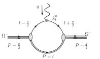
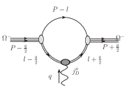
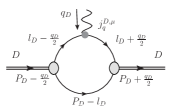
Figure 1: Feynman diagrams for the electromagnetic current of $\Omega^{-}$, (a) and (b), and of the diquark (c). The left and middle panels stand for the contributions of quark (single line) and diquark (double line) to $\Omega^{-}$, respectively.

Thus, the matrix element is expressed as the sum of the quark and diquark contributions as

$$\left\langle p^{\prime},\lambda^{\prime}\left|\hat{J}^{\mu}(0)\right|p,\lambda\right\rangle=\left\langle p^{\prime},\lambda^{\prime}\left|\hat{J}^{\mu}_{q}(0)\right|p,\lambda\right\rangle+\left\langle p^{\prime},\lambda^{\prime}\left|\hat{J}^{\mu}_{D}(0)\right|p,\lambda\right\rangle.$$ (15)

One can get the quark contribution from the Feynman diagram 1 (a) as

$$\begin{split}\left\langle p^{\prime},\lambda^{\prime}\left|\hat{J}^{\mu}_{q}(0)\right|p,\lambda\right\rangle=&-Q^{e}_{q}e\bar{u}_{\alpha^{\prime}}(p^{\prime},\lambda^{\prime}){\left(-ic^{2}\right)}\\ \leavevmode\nobreak\ \leavevmode\nobreak\ \leavevmode\nobreak\ &\times\int\frac{d^{4}l}{(2\pi)^{4}}\frac{1}{\mathfrak{D}}\Gamma^{\alpha^{\prime}\beta^{\prime}}\left(\not{l}+\frac{\not{q}}{2}+m_{q}\right)g_{\beta^{\prime}\beta}\gamma^{\mu}\left(\not{l}-\frac{\not{q}}{2}+m_{q}\right)\Gamma^{\alpha\beta}u_{\alpha}(p,\lambda),\end{split}$$ (16)

where $Q_{q}^{e}$ is the electric charge number carried by the quark participating in the interaction and

$$\begin{split}\mathfrak{D}=&[\left(l-P\right)^{2}-m_{R}^{2}+i\epsilon]^{2}[\left(l-P\right)^{2}-m_{D}^{2}+i\epsilon]\\ &\times\biggl{[}\left(l-\frac{q}{2}\right)^{2}-m_{R}^{2}+i\epsilon\biggr{]}\biggl{[}\left(l+\frac{q}{2}\right)^{2}-m_{R}^{2}+i\epsilon\biggr{]}\biggl{[}\left(l+\frac{q}{2}\right)^{2}-m_{q}^{2}+i\epsilon\biggr{]}\biggl{[}\left(l-\frac{q}{2}\right)^{2}-m_{q}^{2}+i\epsilon\biggr{]}.\end{split}$$ (17)

In Eq. (16), the effective vertex is employed as

$$\Gamma^{\alpha\beta}=g^{\alpha\beta}+c_{2}\gamma^{\beta}\Lambda^{\alpha}+c_{3}\Lambda^{\beta}\Lambda^{\alpha},$$ (18)

where $\Lambda$ is the relative momentum between the quark and diquark, and the superscript $\alpha$ ($\beta$) represents the index of the $\Omega^{-}$ (diquark). $m_{q}$ and $m_{D}$ are the masses of the quark and the diquark, respectively. The couplings, $c_{2}$ and $c_{3}$ can be determined by fitting to the LQCD results of EMFFs. To avoid the loop integral divergence, we employ one simple regularization at each vertex, i.e. we add a scalar function

$$\Xi(p_{1},p_{2})=\frac{c}{[p_{1}^{2}-m_{R}^{2}+i\epsilon][p_{2}^{2}-m_{R}^{2}+i\epsilon]},$$ (19)

where $m_{R}$ is a cutoff mass parameter. In Eq. (19) the parameter $c$ is fixed in order to give the electric charge number of $\Omega^{-}$ at $t=0$. It should be mentioned that this simplification may break the gauge invariant slightly, however it is simpler than other sophisticated methods, such as the Pauli-Villars regularization [74].

According to Fig. 1 (b), the diquark contribution can be expressed as

$$\left\langle p^{\prime},\lambda^{\prime}\left|\hat{J}^{\mu}_{D}(0)\right|p,\lambda\right\rangle=-Q^{e}_{D}e\bar{u}_{\alpha^{\prime}}(p^{\prime},\lambda^{\prime}){ic^{2}}\int\frac{d^{4}l}{(2\pi)^{4}}\frac{1}{\mathfrak{D}^{\prime}}\Gamma^{\alpha^{\prime}}_{\leavevmode\nobreak\ \beta^{\prime}}\left(\not{P}-\not{l}+m_{q}\right)j_{D}^{\mu,\beta^{\prime}\beta}\Gamma^{\leavevmode\nobreak\ \alpha}_{\beta}u_{\alpha}(p,\lambda),$$ (20)

where $Q_{D}^{e}$ is the electric charge number carried by the diquark. The diquark electromagnetic current then can be calculated explicitly from Fig. 1 (c) as

$$\sum_{q}\left\langle p_{D}^{\prime},\lambda_{D}^{\prime}\left|\hat{J}^{\mu}_{q}(0)\right|p_{D},\lambda_{D}\right\rangle=-\epsilon^{*}_{\beta^{\prime}}\left(p_{D}^{\prime},\lambda_{D}^{\prime}\right)j_{D}^{\mu,\beta^{\prime}\beta}\epsilon_{\beta}\left(p_{D},\lambda_{D}\right),$$ (21)

where $\epsilon_{\beta}\left(p_{D},\lambda_{D}\right)$ is the spin-1 diquark field and we simply assume that the axival-vector diquark is on-shell. The calculation details of Eq. (21) are referred to Ref. [67].

Finally, the calculation of the GFFs of the $\Omega^{-}$ hyperon is similar to that of EMFFs replacing the electromagnetic current $j^{\mu}$ by the EMT current $T^{\mu\nu}$ [67].

3 Numerical results

3.1 Determination of parameters

We know that the formal FFs should be extracted from the integral in Eqs. (16) and (20) by using the on-shell identities of the Rarita-Schwinger fields [70, 67]. Moreover, we also need to input the $\Omega^{-}$ mass $M$, $s$ quark mass $m_{q}$, and diquark mass $m_{D}$ as the model parameters. To ensure that $\Omega^{-}$ and the diquark are bound states, $M$, $m_{q}$, and $m_{D}$ need to satisfy the relation, $M<m_{q}+m_{D}<3m_{q}$. Here, we choose $M=1.672\leavevmode\nobreak\ \text{GeV}$ [75], $m_{q}=0.6\leavevmode\nobreak\ \text{GeV}$, and $m_{D}=1.15\leavevmode\nobreak\ \text{GeV}$. In addition, other model parameters, the cutoff mass $m_{R}$ and the couplings $c_{2(3)}$ in Eqs.(17-19), can be modulated to obtain more reasonable form factors, comparing to those of the LQCD calculations. Thus, we finally choose $m_{R}=2.2\,\text{GeV}\gtrsim M$, $c_{2}=0.306\,\text{GeV}^{-1}$, and $c_{3}=0.056\text{GeV}^{-2}$. These three parameters and the input masses are listed in Table 1.

$M/\text{GeV}$	$m_{q}/\text{GeV}$	$m_{D}/\text{GeV}$	$m_{R}/\text{GeV}$	$c_{2}/\text{GeV}^{-1}$	$c_{3}/\text{GeV}^{-2}$
1.672	0.6	1.15	2.2	0.306	0.056

Table 1: The parameters used in this work.

Figure 2 gives the comparison of our electric form factor $G_{E0}$ to the results of LQCD [52] with different $m_{R}$. We conclude that the results are not sensitive to the parameter $m_{R}$.

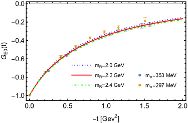
Figure 2: The comparison of $G_{E0}$ with LQCD to different $m_{R}$ when $c_{2}=0.306\,\text{GeV}^{-1}$ and $c_{3}=0.056\text{GeV}^{-2}$.

Furthermore, we find that the parameters $c_{2(3)}$ make a significant impact on the high-order multipoles form factors, such as the electric-quadrupole, magnetic-octupole, energy-quadrupole, and angular momentum-octupole form factors as discussed in Ref. [67], especially on even higher-order multipole magnetic and angular momentum -octupole form factors.

3.2 Results of EMFFs of the $\Omega^{-}$ hyperon

Once the parameters are determined, the EMFFs of $\Omega^{-}$, including the electric-monopole, magnetic-dipole, electric-quadrupole and magnetic-octupole form factors, can be calculated. Our results are compared with the LQCD calculations [52] in Fig. 3. In the Fig. 3, the contributions from the quark and diquark are explicitly displayed. We find that both our calculation and LQCD result are consistent with each other. In particular, our electric-monopole and magnetic-dipole form factors match the LQCD results better. Since the electric charge carried by the diquark is twice that of the quark, the ratio between the diquark and quark contributions is about $2$, as $-t$ tends to $0$. In the forward limit, Fig. 3 gives the magnetic moment $\mu_{\Omega^{-}}=G_{M1}\frac{M_{N}}{M}\mu_{N}$, electric-quadrupole moment $\mathcal{Q}_{\Omega^{-}}=G_{E2}(0)\frac{\lvert e\rvert}{M^{2}}$, and magnetic-octupole moment $\mathcal{O}_{\Omega^{-}}=G_{M3}(0)(\frac{M_{N}}{M})^{3}\mathcal{O}_{N}$. The physical quantities of $\mu_{N}$ and $\mathcal{O}_{N}$ with the subscript $N$ stand for the corresponding nuclear properties and $M_{N}$ being the proton mass. A comparison of our results with those of the different models is also shown in Tab. 2.

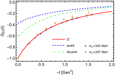
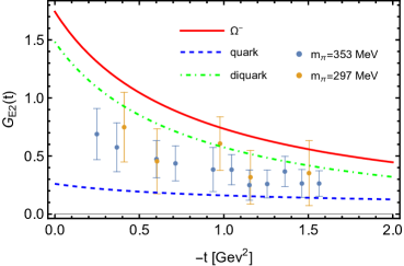
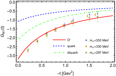
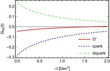
Figure 3: Our EMFFs in comparison with the results of LQCD [52]. The dashed, dotted-dashed and solid lines represent the quark, diquark, and total contributions, respectively.

From Tab. 2, we see that our magnetic moment $\mu_{\Omega^{-}}=-1.8\,\mu_{N}$ is slightly less than the experiment value $-2.02(5)\,\mu_{N}$ and is close to the LQCD and $\chi$QSM results. Moreover, our electric-quadrupole moment is of the same order as others. We know that the electric-quadrupole form factors show the 3D electric charge distribution shape of the system, and $\mathcal{Q}_{\Omega^{-}}>0$ implies that the electric charge distribution of $\Omega^{-}$ is a prolate ellipsoid. In addition, the electromagnetic radii from  (3) are important quantities for us to apprehend the electromagnetic properties of the system, and they are

$$\langle r^{2}\rangle_{E0}=0.352\,\text{fm}^{2}\quad\text{and}\quad\langle r^{2}\rangle_{M1}=0.322\,\text{fm}^{2},$$ (22)

for the $\Omega^{-}$ hyperon. Our results are comparable with other model calculations as shown in the Tab. 2. One can conclude that the magnetic radius is smaller than the electric charge radius and this relation is also in agreement with other model predictions except for the RQM calculation [64].

	$\mu_{\Omega^{-}}/\mu_{N}$	$\mathcal{Q}_{\Omega^{-}}/\text{fm}^{2}$	$\mathcal{O}_{\Omega^{-}}/\mathcal{O}_{N}$	$\langle r^{2}\rangle_{E0}/\text{fm}^{2}$	$\langle r^{2}\rangle_{M1}/\text{fm}^{2}$
this work	-1.8	0.024	-0.008	0.352	0.322
PDG [75]	-2.02(5)	-	-	-	-
LQCD [51]	-1.73(22)	0.0042(56)	$-9.989\pm 2.65$	0.226(16)	0.226(16)
LQCD [52]	-1.835(94)	0.0133(57)	-	0.355(14)	0.286(31)
LQCD [53]	-1.697(65)	0.0086(12)	0.2(1.2)	0.307(15)	-
$\chi$PT [57]	-1.94(22)	0.009(5)	-	-	-
$\chi$PT [58]	-2.02(5)	-	-	0.70(12)	-
$1/N_{c}$ [59, 60]	-1.94	0.018	-0.65	-	-
RQM [64]	-2.02(5)	-	-	0.22	0.27
QCDSR [33]	-1.49(45)	-	-	-	-
QCDSR [76]	-	0.12(4)	1.73(43)	-	-
NRQM [66]	-	0.028	-	-	-
$\chi$QM [54]	-2.13	0.026	-	0.61	0.53
$\chi$QSM [37, 77]	-1.82	0.054	-	0.832	0.582

Table 2: The magnetic moment, electric-quadrupole moment, magnetic-octupole moment, electric charge radius and magnetic radius in comparison with those from PDG [75], LQCD [51, 52, 53], $\chi$PT [57, 58], $1/N_{c}$ expansion [59, 60], relativistic quark model [64], non-relativistic quark model [66], QCD sum rules [33, 76], $\chi$ quark model [54], and chiral quark-soliton model [37, 77].

3.3 Results of GMFFs of $\Omega^{-}$ baryon

Analogously, the matrix element of energy-momentum tensor gives GMFFs, which are expressed in terms of GFFs using the linear components in the Breit frame. By employing the same parameters and the same normalization, the GMFFs, including the energy-monopole $\varepsilon_{0}$, angular momentum-dipole $\mathcal{J}_{1}$, energy-quadrupole $\varepsilon_{2}$, angular momentum-octupole $\mathcal{J}_{3}$ form factors, and some other form factors such as $D_{0}$, $D_{2}$ and $D_{3}$, which may relate to the pressures and shear forces, can be obtained and the their low-order multipole terms are shown in Fig. 4.

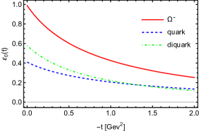
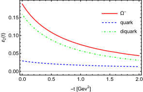
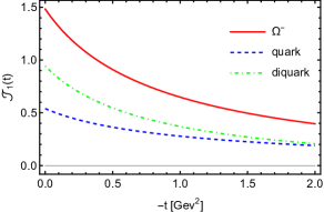
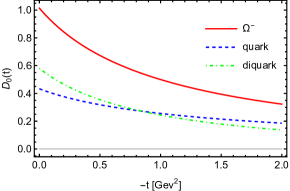
Figure 4: The low order terms of the gravitational form factors of $\Omega^{-}$ as the functions of the squared momentum transfer $t$.

In the forward limit $t=0$, the intrinsic mechanical properties of the $\Omega^{-}$ hyperon, like its mass, $\varepsilon_{0}(0)=0.988\sim 1$, and spin, $\mathcal{J}_{1}(0)=1.483\sim 3/2$, can be obtained in this approach. It is clearly seen that our obtained mass and spin are not the same as the exactly global physical quantities because the momentum-dependence regularization in Eq. (19) violates the gauge invariance slightly. Similar to EMFFs, we find that the ratios between the diquark and quark contributions to the energy-monopole and to the angular momentum-dipole form factors are close to 2, especially for the small $-t$. This is intuitive because the mass and spin of the quark are practically about half of the diquark. It should be stressed that the shape of the energy distribution is another important property, thereupon we can conclude that the $\Omega^{-}$ is a prolate ellipsoid because of the positive $\varepsilon_{2}(0)$. Finally, we get the mass radius of the $\Omega^{-}$ hyperon as

$$\langle r^{2}\rangle_{M}=0.297\,\text{fm}^{2}$$ (23)

from Eq. (6). It is found that this mass radius is slightly smaller than the electromagnetic radii, $\langle r^{2}\rangle_{E0}$ and $\langle r^{2}\rangle_{M1}$, like our calculation for the $\Delta$ resonances [67].

Finally, the $D$-term is also an essential mechanical quantity, which is defined as $D=D_{0}(0)$ and is argued to be negative and closely related to the stability of the system [78]. Here, we get $D\sim 1.01$. It is positive and similar to the value for the $\Delta$ resonance in our previous calculation [67]. The possible interpretation of the positive $D$-term will be discussed in the following subsection.

3.4 GMFFs in $r$-space

The local density distributions, including the energy densities (9), angular momentum density (14), and the internal forces (11), can be obtained from the Fourier transformed form factors. To consider local particles, we simply employ a wave packet to describe the $\Omega^{-}$ hyperon. It should be addressed that Ref. [79] concludes that the local density distributions must depend on the wave packet. Here, we simply employ an additional Gaussian-like wave packet $e^{\frac{t}{\lambda^{2}}}$ to describe the system [80] as an approximation in Eqs.(10,12,14). In addition, this description can also guarantee the good convergence in the Fourier transformations. This additional wave packet may affect the radius definition [79, 81], however, this issue is not a priority in this work.

It should be mentioned that the parameter $1/\lambda$ here characterizes the size of $\Omega^{-}$ and $\lambda$ has the mass dimension. Thus, one can conclude that the large $\lambda$ represents the small radius (the small $\lambda$ is opposite) according to the uncertainty principle. Thereupon the large $\lambda$ concentrates the densities close to the center (small $r$ region) and the small $\lambda$ to the contrary as shown in Fig. 5,

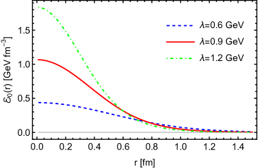
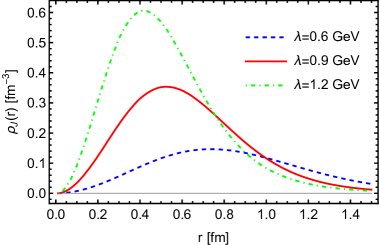
Figure 5: The calculated energy-monopole (left panel) and angular momentum (right) densities of $\Omega^{-}$ as the functions of $r$ with different $\lambda$.

where we choose the reasonable $\lambda$ range $0.6\,\text{GeV}<\lambda<1.2\,\text{GeV}$. Furthermore, there are certainly some invariants in the energy and angular momentum densities in Fig. 5. For example, the integrated result of $\rho_{J}(r)$ in the 3D coordinate space corresponds to the total spin and is independent of $\lambda$, and the integrated result of $\varepsilon_{0}(r)$ gives the mass term. Note that $\lambda=0.9\,\text{GeV}$ is employed in the following discussion.is not a priority

The energy density in 3D space, from Eq. (7) taking the polarization average, is shown in Fig. 6. One sees that the energy distribution has a prolate shape due to the positive energy-quadrupole form factor mentioned above.

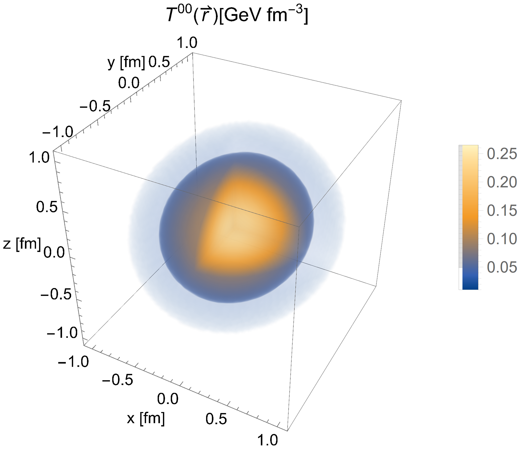
Figure 6: The energy density using the polarization average.

The next relevant part is the $ij$-component of the static EMT, which describes the so-called pressures $p_{n}(r)$ and shear forces $s_{n}(r)$ argued in Refs. [11, 78] and is related to the GFFs. According to Eq. (11), the pressure and shear force are shown in Fig. 7 and they satisfy the equilibrium relation (13). In the left panel of Fig. 7, there is a crossing at about $r\sim 0.6\,\text{fm}$, which is slightly larger than the mass radius and depends on $\lambda$. We conclude that that $r\sim 0.6\,\text{fm}$ represents that there is a change in the pressure direction at the particle boundary.

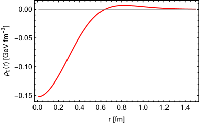
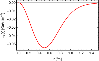
Figure 7: The pressure (left panel) and shear force (right panel) of $\Omega^{-}$ as functions of $r$ when $\lambda=0.9\,\text{GeV}$.

Ref. [78] stressed that the $D$-term is a fundamental and unknown quantity. It represents the stability of the system. The $D$-term is negativity since the corresponding inner force must be outward [78], i.e.

$$p_{0}(r)+\frac{2}{3}\,s_{0}(r)>0.$$ (24)

Thus, the positive $D$ term in our approach may imply that $\Omega^{-}$ is not be stable according to the above point of view of Ref. [78]. We claim that we have demonstrated that the positive $D$-term for the $\Delta$ resonance in our quark-diquark approach [67]. Note that the similar positive $D$-term is also obtained in the calculation of hydrogen atom in Ref. [82]. Although our result does not satisfy the inequality of (24), the von Laue condition is indeed satisfied

$$\int^{\infty}_{0}drr^{2}p_{0}(r)=0,$$ (25)

which can be elucidated by Fig. 8, where the equality between the areas of the upper and lower shaded parts is shown.

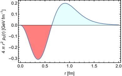
Figure 8: The physical quantity $4\pi r^{2}p_{0}(r)$ as a function of $r$.

To explore the $\Omega^{-}$ stability in more detail, we plot the momentum current distribution on the $x-y$ plane with $z=0$ in Fig. 9 according to Eq. (8), where the arrows and shades represent its direction and strength, respectively. It is clearly seen that the absolute value of the momentum current at boundary is close to zero. Thus, Fig. 9 implies that this is a stable system. If we add a minus sign to $D_{0}(t)$ by hand, the negative $D$-term is obtained and only the arrow of each point in Fig. 9 points to the opposite direction according to Eq. (11), but one can find that the system is also stable. Therefore, we argue that the stability is independent of the sign of the $D$-term, i.e. there is no direct relation between the stability of a hadron and the sign of the $D$-term as also have been discussed in Ref. [82].

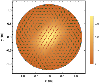
Figure 9: The momentum current with the unit $\text{GeV fm}^{-3}$ on the $x-y$ plane with $z=0$.

4 Summary and discussion

In this work, the electromagnetic and gravitational form factors of $\Omega^{-}$ hyperon have been calculated simultaneously using the quark-diquark approach. The diquark with two $s$ quarks is considered as an axial-vector particle and its specific inner structure is also considered when we discuss the $\Omega^{-}$ form factors. In our calculation, we use the effective vertex between the hadron and two effective partons, quark and diquark, and the simple regularization is also employed to make the integral convergence. The model parameters are determined by fitting our EMFFs to the LQCD results.

Our obtained electromagnetic properties of the $\Omega^{-}$ hyperon, such as its magnetic moment, electric-quadrupole moment, electromagnetic radii, and so on, are in a reasonable agreement with those of the experiments, LQCD calculations, and other models. In addition, we find that the mass radius is smaller than the electromagnetic radii. Compared to the results of the $\Delta$ resonance, we conclude that $\Omega^{-}$ has the smaller electromagnetic and mass radii due to the stronger boundary. Because of the similar quark components, the behaviours of $\Omega^{-}$ and $\Delta^{++}$ form factors are similar for the low-order ones and the energy distribution takes the same prolate shape which can also be illustrated by the positive $\varepsilon_{2}(0)$.

The energy density, angular momentum density, and internal forces including pressures and shear forces are also given in the coordinate space by the Fourier transformed form factors. An important and fundamental property of the system is its stability, and Ref. [11] argued that the stable system must have the negative $D$-term. However, this explanation is still controversial [11, 82, 22]. According to our calculations and analyses of GFFs, we believe that there are three important issues that need to be stressed and studied.

1. There should be mechanical stability and decay stability. The former is due to the resultant force being zero at any point and represents the existence of the particle, and the latter is because of the forbiddance of its strong decay and represents, at least to some extend, the lifetime of the particle. We believe that it is important to distinguish between these two types of the stability. The stability, discussed in Ref. [11] and the related work including this work, should be mechanical stability. We argue that all the existent particles, including the unstable particles, even with strong decay modes such as $\Delta$ resonances, need to be mechanically stable during their existence.

2. In this work, the FFs are calculated under the premise that $\Omega^{-}$ is a three quark bound state. We argue that there might be no classical pressure and shear force in this few-body and hadronic system as well as in the hydrogen atom system [82], because the pressure and shear force result from the statistical mean in the multi-body systems. In our opinion, it is more reasonable to use the momentum current $T^{ij}(\bm{r})$ as a criterion to judge the mechanical stability, because the momentum current does exist in any kind of system.

3. Moreover, the FFs describe the static properties of the particle in general, and they must give a mechanically stable result if the particle exists. As mentioned above and explicitly addressed in Ref. [67] and this work, we obtain the positive $D$-term for the spin-3/2 particles of $\Delta$ resonances and $\Omega^{-}$ hyperon in the covariant quark-diquark approach. What’s the most important is that the obtained momentum flux on any small volume is zero whether the $D$-term is positive or negative according to our analyses. Therefore, we conclude that the mechanical stability does not relate to the sign of the $D$-term.

References

- [1] Ronald A. Gilman and Franz Gross. Electromagnetic structure of the deuteron. J. Phys. G, 28:R37–R116, 2002.
- [2] Franz Gross. Electromagnetic structure of the deuteron: Review of recent theoretical and experimental results. Eur. Phys. J. A, 17:407–413, 2003.
- [3] Yu-bing Dong, Amand Faessler, Thomas Gutsche, and Valery E. Lyubovitskij. Phenomenological Lagrangian approach to the electromagnetic deuteron form factors. Phys. Rev. C, 78:035205, 2008.
- [4] J. P. B. C. de Melo, T. Frederico, E. Pace, S. Pisano, and G. Salme. Time- and Spacelike Nucleon Electromagnetic Form Factors beyond Relativistic Constituent Quark Models. Phys. Lett. B, 671:153–157, 2009.
- [5] Ian C. Cloët, Wolfgang Bentz, and Anthony W. Thomas. Role of diquark correlations and the pion cloud in nucleon elastic form factors. Phys. Rev. C, 90:045202, 2014.
- [6] Bao-dong Sun and Yu-bing Dong. Deuteron electromagnetic form factors with the light-front approach. Chin. Phys. C, 41(1):013102, 2017.
- [7] M. V. Polyakov. Generalized parton distributions and strong forces inside nucleons and nuclei. Phys. Lett. B, 555:57–62, 2003.
- [8] S. Kumano, Qin-Tao Song, and O. V. Teryaev. Hadron tomography by generalized distribution amplitudes in pion-pair production process and gravitational form factors for pion. Phys. Rev. D, 97(1):014020, 2018.
- [9] Maxim V. Polyakov and Hyeon-Dong Son. Nucleon gravitational form factors from instantons: forces between quark and gluon subsystems. JHEP, 09:156, 2018.
- [10] Cédric Lorcé, Hervé Moutarde, and Arkadiusz P. Trawiński. Revisiting the mechanical properties of the nucleon. Eur. Phys. J. C, 79(1):89, 2019.
- [11] Maxim V. Polyakov and Peter Schweitzer. Forces inside hadrons: pressure, surface tension, mechanical radius, and all that. Int. J. Mod. Phys. A, 33(26):1830025, 2018.
- [12] G. Hohler and E. Pietarinen. Electromagnetic Radii of Nucleon and Pion. Phys. Lett. B, 53:471–475, 1975.
- [13] Pieter Maris and Peter C. Tandy. The pi, K+, and K0 electromagnetic form-factors. Phys. Rev. C, 62:055204, 2000.
- [14] Adam M. Bincer. Electromagnetic structure of the nucleon. Phys. Rev., 118:855–863, 1960.
- [15] Hirotaka Sugawara and Frank Von Hippel. Zero-Parameter Model of the N-N Potential. Phys. Rev., 172:1764–1788, 1968.
- [16] V. D. Burkert, L. Elouadrhiri, and F. X. Girod. The pressure distribution inside the proton. Nature, 557(7705):396–399, 2018.
- [17] V. D. Burkert, L. Elouadrhiri, F. X. Girod, C. Lorcé, P. Schweitzer, and P. E. Shanahan. Colloquium: Gravitational Form Factors of the Proton. 3 2023.
- [18] Bao-Dong Sun and Yu-Bing Dong. meson unpolarized generalized parton distributions with a light-front constituent quark model. Phys. Rev. D, 96(3):036019, 2017.
- [19] Edgar R. Berger, F. Cano, M. Diehl, and B. Pire. Generalized parton distributions in the deuteron. Phys. Rev. Lett., 87:142302, 2001.
- [20] F. Cano and B. Pire. Deep electroproduction of photons and mesons on the deuteron. Eur. Phys. J. A, 19:423–438, 2004.
- [21] Yubing Dong and Cuiying Liang. Generalized parton distribution functions of a deuteron in a phenomenological Lagrangian approach. J. Phys. G, 40:025001, 2013.
- [22] June-Young Kim, Bao-Dong Sun, Dongyan Fu, and Hyun-Chul Kim. Mechanical structure of a spin-1 particle. Phys. Rev. D, 107(5):054007, 2023.
- [23] T. K. Pedlar et al. Precision measurements of the timelike electromagnetic form-factors of pion, kaon, and proton. Phys. Rev. Lett., 95:261803, 2005.
- [24] Kamal K. Seth, S. Dobbs, Z. Metreveli, A. Tomaradze, T. Xiao, and G. Bonvicini. Electromagnetic Structure of the Proton, Pion, and Kaon by High-Precision Form Factor Measurements at Large Timelike Momentum Transfers. Phys. Rev. Lett., 110(2):022002, 2013.
- [25] S. Dobbs, A. Tomaradze, T. Xiao, Kamal K. Seth, and G. Bonvicini. First measurements of timelike form factors of the hyperons, , , , , , and , and evidence of diquark correlations. Phys. Lett. B, 739:90–94, 2014.
- [26] M Andreotti et al. Measurements of the magnetic form-factor of the proton for timelike momentum transfers. Phys. Lett. B, 559:20–25, 2003.
- [27] Xiang-Dong Ji. Off forward parton distributions. J. Phys. G, 24:1181–1205, 1998.
- [28] K. Goeke, Maxim V. Polyakov, and M. Vanderhaeghen. Hard exclusive reactions and the structure of hadrons. Prog. Part. Nucl. Phys., 47:401–515, 2001.
- [29] Matthias Burkardt. Impact parameter space interpretation for generalized parton distributions. Int. J. Mod. Phys. A, 18:173–208, 2003.
- [30] M. Diehl. Generalized parton distributions. Phys. Rept., 388:41–277, 2003.
- [31] A. V. Belitsky and A. V. Radyushkin. Unraveling hadron structure with generalized parton distributions. Phys. Rept., 418:1–387, 2005.
- [32] Felix Schlumpf. Magnetic moments of the baryon decuplet in a relativistic quark model. Phys. Rev. D, 48:4478–4480, 1993.
- [33] Frank X. Lee. Determination of decuplet baryon magnetic moments from QCD sum rules. Phys. Rev. D, 57:1801–1821, 1998.
- [34] Jishnu Dey, Mira Dey, and Ashik Iqubal. Magnetic moment of the Omega- in QCD sum rule (QCDSR). Phys. Lett. B, 477:125–129, 2000.
- [35] Alfons J. Buchmann and Richard F. Lebed. Baryon charge radii and quadrupole moments in the 1/N(c) expansion: The three flavor case. Phys. Rev. D, 67:016002, 2003.
- [36] Soon-Tae Hong. Sum rules for baryon decuplet magnetic moments. Phys. Rev. D, 76:094029, 2007.
- [37] June-Young Kim and Hyun-Chul Kim. Electromagnetic form factors of the baryon decuplet with flavor SU(3) symmetry breaking. Eur. Phys. J. C, 79(7):570, 2019.
- [38] June-Young Kim and Bao-Dong Sun. Gravitational form factors of a baryon with spin-3/2. Eur. Phys. J. C, 81(1):85, 2021.
- [39] C. Aubin, K. Orginos, V. Pascalutsa, and M. Vanderhaeghen. Magnetic Moments of Delta and Omega- Baryons with Dynamical Clover Fermions. Phys. Rev. D, 79:051502, 2009.
- [40] C. Alexandrou, T. Korzec, G. Koutsou, Th. Leontiou, C. Lorce, J. W. Negele, V. Pascalutsa, A. Tsapalis, and M. Vanderhaeghen. Delta-baryon electromagnetic form factors in lattice QCD. Phys. Rev. D, 79:014507, 2009.
- [41] June-Young Kim. Quark distribution functions and spin-flavor structures in transitions. 5 2023.
- [42] G. Ramalho. Electromagnetic form factors of the baryon in the spacelike and timelike regions. Phys. Rev. D, 103(7):074018, 2021.
- [43] Bernard Aubert et al. A Study of using initial state radiation with BABAR. Phys. Rev. D, 73:012005, 2006.
- [44] Bernard Aubert et al. Study of , , using initial state radiation with BABAR. Phys. Rev. D, 76:092006, 2007.
- [45] Medina Ablikim et al. Observation of a cross-section enhancement near mass threshold in . Phys. Rev. D, 97(3):032013, 2018.
- [46] Medina Ablikim et al. Measurements of and time-like electromagnetic form factors for center-of-mass energies from 2.3864 to 3.0200 GeV. Phys. Lett. B, 814:136110, 2021.
- [47] Chang-Zheng Yuan and Marek Karliner. Cornucopia of Antineutrons and Hyperons from a Super J/ Factory for Next-Generation Nuclear and Particle Physics High-Precision Experiments. Phys. Rev. Lett., 127(1):012003, 2021.
- [48] S. Dobbs, Kamal K. Seth, A. Tomaradze, T. Xiao, and G. Bonvicini. Hyperon Form Factors & Diquark Correlations. Phys. Rev. D, 96(9):092004, 2017.
- [49] B. Singh et al. Feasibility study for the measurement of transition distribution amplitudes at ANDA in . Phys. Rev. D, 95(3):032003, 2017.
- [50] A. W. Chan et al. Measurement of the Properties of the and hyperons. Phys. Rev. D, 58:072002, 1998.
- [51] Derek B. Leinweber, Terrence Draper, and R. M. Woloshyn. Decuplet baryon structure from lattice QCD. Phys. Rev. D, 46:3067–3085, 1992.
- [52] C. Alexandrou, T. Korzec, G. Koutsou, J. W. Negele, and Y. Proestos. The Electromagnetic form factors of the in lattice QCD. Phys. Rev. D, 82:034504, 2010.
- [53] S. Boinepalli, D. B. Leinweber, P. J. Moran, A. G. Williams, J. M. Zanotti, and J. B. Zhang. Precision electromagnetic structure of decuplet baryons in the chiral regime. Phys. Rev. D, 80:054505, 2009.
- [54] G. Wagner, A. J. Buchmann, and A. Faessler. Electromagnetic properties of decuplet hyperons in a chiral quark model with exchange currents. J. Phys. G, 26:267–293, 2000.
- [55] Wojciech Broniowski and Enrique Ruiz Arriola. Gravitational and higher-order form factors of the pion in chiral quark models. Phys. Rev. D, 78:094011, 2008.
- [56] June-Young Kim, Hyun-Chul Kim, Maxim V. Polyakov, and Hyeon-Dong Son. Strong force fields and stabilities of the nucleon and singly heavy baryon . Phys. Rev. D, 103(1):014015, 2021.
- [57] Malcolm N. Butler, Martin J. Savage, and Roxanne P. Springer. Electromagnetic moments of the baryon decuplet. Phys. Rev. D, 49:3459–3465, 1994.
- [58] Hao-Song Li, Zhan-Wei Liu, Xiao-Lin Chen, Wei-Zhen Deng, and Shi-Lin Zhu. Magnetic moments and electromagnetic form factors of the decuplet baryons in chiral perturbation theory. Phys. Rev. D, 95(7):076001, 2017.
- [59] Markus A. Luty, John March-Russell, and Martin J. White. Baryon magnetic moments in a simultaneous expansion in 1/N and m(s). Phys. Rev. D, 51:2332–2337, 1995.
- [60] Alfons J. Buchmann. Electromagnetic Multipole Moments of Baryons. Few Body Syst., 59(6):145, 2018.
- [61] Hyun-Chul Kim, Peter Schweitzer, and Ulugbek Yakhshiev. Energy-momentum tensor form factors of the nucleon in nuclear matter. Phys. Lett. B, 718:625–631, 2012.
- [62] Matt J. Neubelt, Andrew Sampino, Jonathan Hudson, Kemal Tezgin, and Peter Schweitzer. Energy momentum tensor and the D-term in the bag model. Phys. Rev. D, 101(3):034013, 2020.
- [63] K. Azizi and U. Özdem. Nucleon’s energy–momentum tensor form factors in light-cone QCD. Eur. Phys. J. C, 80(2):104, 2020.
- [64] G. Ramalho, K. Tsushima, and Franz Gross. A Relativistic quark model for the Omega- electromagnetic form factors. Phys. Rev. D, 80:033004, 2009.
- [65] Nathan Isgur, Gabriel Karl, and Roman Koniuk. D Waves in the Nucleon: A Test of Color Magnetism. Phys. Rev. D, 25:2394, 1982.
- [66] M. I. Krivoruchenko and M. M. Giannini. Quadrupole moments of the decuplet baryons. Phys. Rev. D, 43:3763–3765, 1991.
- [67] Dongyan Fu, Bao-Dong Sun, and Yubing Dong. Electromagnetic and gravitational form factors of resonance in a covariant quark-diquark approach. Phys. Rev. D, 105(9):096002, 2022.
- [68] Dongyan Fu, Bao-Dong Sun, and Yubing Dong. Generalized parton distributions in spin-3/2 particles. Phys. Rev. D, 106(11):116012, 2022.
- [69] Dongyan Fu, Bao-Dong Sun, and Yubing Dong. Generalized parton distributions of resonance in a diquark spectator approach. 5 2023.
- [70] Sabrina Cotogno, Cédric Lorcé, Peter Lowdon, and Manuel Morales. Covariant multipole expansion of local currents for massive states of any spin. Phys. Rev. D, 101(5):056016, 2020.
- [71] S. Nozawa and D. B. Leinweber. Electromagnetic form-factors of spin 3/2 baryons. Phys. Rev. D, 42:3567–3571, 1990.
- [72] H. Meyer. The Nucleon as a relativistic quark - diquark bound state with an exchange potential. Phys. Lett. B, 337:37–42, 1994.
- [73] V. Keiner. Electromagnetic form-factors of the nucleon in a covariant diquark model. Z. Phys. A, 354:87, 1996.
- [74] W. Pauli and F. Villars. On the Invariant regularization in relativistic quantum theory. Rev. Mod. Phys., 21:434–444, 1949.
- [75] R. L. Workman et al. Review of Particle Physics. PTEP, 2022:083C01, 2022.
- [76] T. M. Aliev, K. Azizi, and M. Savci. Electric Quadrupole and Magnetic Octupole Moments of the Light Decuplet Baryons Within Light Cone QCD Sum Rules. Phys. Lett. B, 681:240–246, 2009.
- [77] Yu-Son Jun, Hyun-Chul Kim, June-Young Kim, and Jung-Min Suh. Structure of the baryon and the kaon cloud. PTEP, 2022(4):49302, 2022.
- [78] I. A. Perevalova, M. V. Polyakov, and P. Schweitzer. On LHCb pentaquarks as a baryon-(2S) bound state: prediction of isospin- pentaquarks with hidden charm. Phys. Rev. D, 94(5):054024, 2016.
- [79] E. Epelbaum, J. Gegelia, N. Lange, U. G. Meißner, and M. V. Polyakov. Definition of Local Spatial Densities in Hadrons. Phys. Rev. Lett., 129(1):012001, 2022.
- [80] Tomomi Ishikawa, LuChang Jin, Huey-Wen Lin, Andreas Schäfer, Yi-Bo Yang, Jian-Hui Zhang, and Yong Zhao. Gaussian-weighted parton quasi-distribution (Lattice Parton Physics Project (LP3)). Sci. China Phys. Mech. Astron., 62(9):991021, 2019.
- [81] H. Alharazin, B. D. Sun, E. Epelbaum, J. Gegelia, and U. G. Meißner. Local spatial densities for composite spin-3/2 systems. JHEP, 02:163, 2023.
- [82] Xiangdong Ji and Yizhuang Liu. Momentum-Current Gravitational Multipoles of Hadrons. Phys. Rev. D, 106(3):034028, 2022.