An octupolar test of general relativity

Abstract

Compact binaries with unequal masses and whose orbits are not aligned with the observer’s line of sight are excellent probes of gravitational radiation beyond the quadrupole approximation. Among the compact binaries observed so far, strong evidence of octupolar modes is seen in GW190412 and GW190814, two binary black holes observed during the first half of the third observing run of LIGO/Virgo observatories. These two events, therefore, provide a unique opportunity to test the consistency of the octupolar modes with the predictions of general relativity (GR). In the post-Newtonian (PN) approximation to GR, the gravitational-wave phasing has known dependencies on different radiative multipole moments, including the mass octupole. This permits the use of publicly released posteriors of the PN phase deformation parameters for placing constraints on the deformations to the different PN components of the radiative mass octupole denoted by $\delta\mu_{3n}$. Combining the posteriors on $\delta\mu_{3n}$ from these two events, we deduce a joint bound (at 90% credibility) on the first three PN order terms in the radiative octupoles to be $\delta\mu_{30}=-0.07^{+0.11}_{-0.12}$, $\delta\mu_{32}=0.48^{+0.93}_{-1.15}$, and $\delta\mu_{33}=-0.32^{+1.67}_{-0.62}$, consistent with GR predictions. Among these, the measurement of $\delta\mu_{33}$ for the first time confirms the well-known octupolar tail contribution, a novel nonlinear effect due to the scattering of the octupolar radiation by the background spacetime, is consistent with the predictions of GR. Detection of similar systems in the future observing runs should further tighten these constraints.

I Introduction

It is well known that the leading order gravitational wave (GW) emission is quadrupolar according to general relativity. However, subdominant higher multipoles get turned on if the binary has a mass asymmetry and when the line of sight of the observer is not aligned with the orbital angular momentum vector of the binary [1, 2, 3, 4, 5, 6, 7, 8, 9]. To date, the LIGO-Virgo-KAGRA (LVK) Collaboration has reported $\sim$90 confident detections of compact binary mergers [10, 11, 12, 13]. Among these events, two compact binary mergers – GW190412 [14] and GW190814 [15] – have shown clear evidence of the presence of octupolar ($\ell=3,m=3$) mode, the first correction beyond the quadrupole. These two events, therefore, should facilitate a test of the gravitational octupolar structure of the compact binary dynamics.

The gravitational dynamics of a compact binary system is typically divided into three stages of evolution: inspiral, merger, and ringdown. While the post-Newtonian (PN) approximation to general relativity (GR) [16] is employed to model the adiabatic inspiral stage of a compact binary coalescence, one requires numerical solutions to the Einstein equations [17], and the black hole (BH) perturbation theory [18] to describe the highly nonlinear merger stage, and the ringdown phase, respectively. As numerical relativity simulations are computationally expensive, currently there are two main modeling approaches towards producing the complete gravitational waveform (i.e., a single waveform that captures all three stages of binary evolution) for parameter inference: Effective One Body (EOB) approach [19, 20] and Phenomenological approach [21, 22]. Both these methods make the best use of the analytical and numerical understanding of compact binary dynamics.

The gravitational waveform from a coalescing compact binary within GR, in the frequency domain, has the following form

$$\tilde{h}(f;\vec{\lambda},\iota,\varphi_{N})=\sum_{\ell\geq 2}\sum_{m=-\ell}^{\ell}\,Y_{-2}^{\ell m}(\iota,\varphi_{N})\,\tilde{h}_{\ell m}\,(f;\vec{\lambda}),$$ (1)

where $Y_{-2}^{\ell m}$ are spin-weighted spherical harmonics of spin weight $-2$, ($\iota,\varphi_{N}$) describes the location of the observer in the binary’s sky and $\vec{\lambda}$ denotes the intrinsic parameters (e.g., masses and spins) as well as other relevant extrinsic parameters (e.g., luminosity distance ($d_{L}$), reference time and reference phase) of the binary. Each GW mode ($\tilde{h}_{\ell m}$) has an amplitude, $A_{\ell m}(f;\vec{\lambda})$, and a phase, $\psi_{\ell m}(f;\vec{\lambda})$ (i.e., $\tilde{h}_{\ell m}=A_{\ell m}(f;\vec{\lambda})\,e^{i\,\psi_{\ell m}(f;\vec{\lambda})}$). In alternative theories of gravity, the gravitational dynamics of a compact binary could differ from the prediction of GR during all the three stages and might modify the phase and amplitude in the waveform.

There exist proposals in the literature to probe the prediction of the harmonic structure of gravitational radiation from binary black hole coalescence in GR  [23, 24, 25, 26, 27]. Using GW190412 and GW190814, Ref. [28] tested the consistency between the dominant and sub-dominant modes and found the chirp mass estimated from the $\ell=3,m=3$ mode to be within $\pm 1\%$ of the one estimated from the quadrupolar $\ell=2,m=2$ mode.

In a more recent work [29], the consistency of the amplitudes of the $h_{21}$ and $h_{33}$ modes of the GW spectrum with GR predictions was investigated using these two events and found no evidence for any violation of GR. This test assumes the phases of sub-dominant harmonics ($\psi_{\ell m;\ell>2}$) follow GR and investigates whether the amplitudes of sub-dominant harmonics ($A_{\ell m;\ell>2}$) are consistent with the GR prediction.

Parametrized tests of GW phasing that look for potential GR violations in the various PN phasing coefficients [30, 31, 32, 33, 34, 35, 36, 37], have been already applied to the data from these two events [14, 15, 38]. It is shown that the inclusion of higher modes in the waveform model provides better constraints on the parametrized tests of GR [35, 14, 15, 39] (See section VA of Ref. [38]).

In this letter, we argue that if a signal contains nonquadrupolar modes, apart from the amplitude, the phase evolution will also carry their unique imprints [40, 1, 25, 26]. As GW detectors are more sensitive to phase evolution, this could be used to test GR, complementing the approach of [29]. However, we will focus only on the inspiral phase in this work, which is well-modeled by PN approximation to GR, and discuss constraints on the PN structure of octupolar emission in GR. For this, we will make use of the unique map between the mass-type octupole coefficients at different PN orders and the bounds on the 1PN, 2PN, and 2.5PN logarithmic phasing deformation parameters for these two events in the parameterized tests of PN theory reported in [38, 41].

II Parametrized tests of GW phasing

The frequency domain GW phase from the inspiral part of the waveform (computed using the stationary phase approximation [42, 43]) for the leading quadrupolar harmonic [44, 4] takes the form

$$\Psi(f) =2\pi f\,t_{c}-\phi_{c}$$

$$\quad+\frac{3}{128\,\nu\,v^{5}}\left[\,\sum_{i=0}^{i=7}\left(\phi_{i}\,+\phi_{il}\,\ln v\right)v^{i}\,+\mathcal{O}(v^{8})\right]\,,$$ (2)

where $v=(\pi GMf/c^{3})^{1/3}$ is the PN expansion parameter, $M$ is the binary’s redshifted total mass, $\nu$ is the symmetric mass ratio of the binary, $\phi_{i}$ and $\phi_{il}$ denote the non-logarithmic and logarithmic PN phasing coefficients, respectively.

Due to the lack of accurate waveforms in alternative theories of gravity, “theory-agnostic” approaches are often adopted to test GR with GW data. These “null tests” of GR make use of our best knowledge of compact binary dynamics in GR and look for possible deviations from GR without reference to specific alternatives (See Ref [45, 46, 38, 41] for more details.). One of the most generic tests of GR that has been routinely performed with LIGO/Virgo data is the parametrized test of PN theory [30, 31, 32, 33, 34, 35, 36, 37].

The parametrized tests rely on measuring any deviations in the PN coefficients $\phi_{i}$ and $\phi_{il}$ in the GW phasing, which are uniquely predicted by GR, from compact binary mergers. A parametrized waveform model introduces additional degrees of freedom to capture signatures of possible GR violation by modifying the phasing coefficients as

$$\phi_{b}=\phi_{b}^{\rm GR}(1+\delta\hat{\phi}_{b}),$$ (3)

($b=i,\,il$) (see section VA of Refs. [38, 41] for more details). In GR, these phenomenological dimensionless deviation parameters ($\delta\hat{\phi}_{b}$) are identically zero, whereas in alternative theories of gravity, one or more of these parameters could be different from zero. Combining data from different GW events detected during the first, second, and third observing runs of LIGO/Virgo, the current bound on the PN deviation parameters are found to be consistent with GR (see Fig. 6 and Fig. 7 of Ref. [41]).

For the two asymmetric binary events, GW190412 and GW190814, we will use the results of the parametrized tests, obtained by applying parameterized IMRPhenomPv3HM (denoted as “Phenom” in this letter) [8] and SEOBNRv4HM$\_$ROM (denoted as “SEOB”)[9] waveform approximant to the data. Phenom waveform is a frequency-domain phenomenological waveform model that includes the effects of two-spin precession along with higher multipole moments [8], whereas SEOB is a frequency-domain non-precessing reduced-order EOB model that incorporates the higher order modes [9]. In the current LVK analyses [46, 38, 41], the reported bounds on $\delta\hat{\phi}_{b}$ come from the fractional deviations applied to the non-spinning portion of the phase (see Sec. VA of Refs. [38, 41] for detailed discussions).

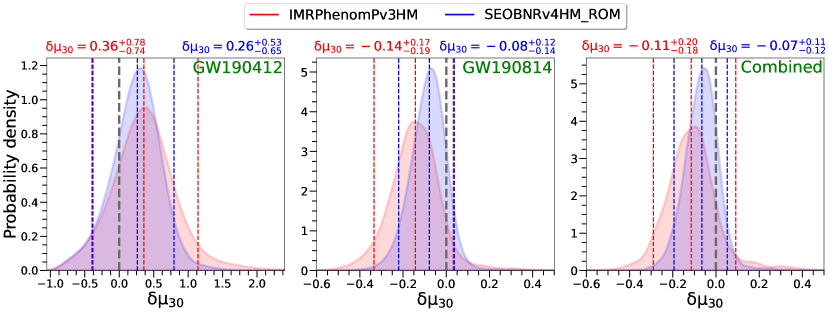
Figure 1: Bounds on $\delta\mu_{30}$ for GW190412 and GW190814 analyzed with Phenom (in red color) and SEOB (in blue color) waveform approximants are shown. Left-most panel shows the bounds for GW190412, whereas the middle panel shows the result for GW190814. The combined bounds are shown in the rightmost panel. The colored vertical dashed lines mark the 90% credible intervals and median values. The gray dashed vertical line indicates the GR prediction ($\delta\mu_{30}=0$). The $\delta\mu_{30}$ posteriors are consistent with GR prediction.

III Parameterized multipolar gravitational waveforms

The radiative multipole moments of a compact binary system contain information about source physics (masses [47, 40, 16], spins [48, 49, 50, 51, 52, 4, 53, 54, 55, 16, 56, 57, 58, 59, 60], tidal deformability [61, 62, 63, 64, 65, 66, 67], spin induced quadrupole moment [51, 68, 69, 70, 71] etc.) and account for various nonlinear interactions and physical effects (such as ‘tail’ effects [72, 73, 40], tails of tails [74], tail square [75], memory effects [76, 77, 78, 79], spin-orbit effects [48, 80], spin-spin effects [48, 59] etc.) that occur at different PN orders in GR. In alternative theories of gravity, one or more radiative multipole moments of a compact binary could be different from those in GR (see for instance Ref. [81]). Such theories can be tested by studying the multipolar structure of asymmetric compact binary systems like GW190412 and GW190814.

Refs. [25, 26] came up with a novel theory-agnostic method to test the multipolar structure of the gravitational field radiated from an inspiralling compact binary. Using the multipolar post-Minkowskian (MPM) formalism [82, 83, 84, 85, 72, 86, 47, 87, 40, 88, 89, 90], Ref. [25] derived the parametrized multipolar gravitational wave phasing up to 3.5PN order for non-spinning binaries and Ref. [26] extended it for non-precessing binaries. The MPM formalism relates the radiation content in the far zone, encoded in the mass- and current-type radiative multipole moments $\{U_{L},V_{L}\}$, to the stress-energy tensor of the source. In order to model possible deviations in the multipole structure, Ref. [25, 26] adopted the following parametrization for radiative multipole moments: $U_{L}\rightarrow\mu_{l}\,U_{L}$, $V_{L}\rightarrow\epsilon_{l}\ V_{L}$. By construction, the phenomenological multipole parameters $\mu_{l}$, $\epsilon_{l}$ are equal to unity in GR. With this parametrization, the contributions from various radiative multipole moments to the GW phasing can be tracked separately, thereby facilitating tests of the multipolar structure of the PN approximation to GR.

In this work, we go one step further and probe the different PN orders in the radiative mass octupole moment of a compact binary as it evolves through the adiabatic inspiral phase. We propose the parametrization

$$U_{ijk}\longrightarrow\sum_{n}\frac{1}{c^{n}}\,\mu_{3n}\,U_{ijk}^{(n),{\rm GR}}\,,$$ (4)

where, $U_{ijk}$ is the mass type radiative octupole moment, $U_{ijk}^{(n),{\rm GR}}$ is the (n/2)-th PN correction to $U_{ijk}$ in GR and $\mu_{3n}$ is the corresponding octupole coefficient. Note that there is no 1/c (i.e., 0.5 PN) contribution in the mass octupole moment in GR. The 1.5PN correction term in the octupole moment arises due to the tail effect, caused by the scattering of the outgoing octupolar wave off the background spacetime associated with the total (ADM) mass of the source [72, 73, 40, 74, 75]. By definition $\mu_{3n}$ is unity in GR and appears at different PN orders in the phasing formula. For instance, $\mu_{30}$ first appears at 1PN, $\mu_{32}$ at 2PN and $\mu_{33}$ at 2.5PN. We next discuss how the existing bounds on the PN deformation coefficients $\delta\hat{\phi}_{b}$, based on the parametrization in Eq. 3, reported in [38, 41] can be mapped to the bounds on $\mu_{3n}$ in the parametrization derived above.

Figure 2: The posterior probability distributions on $\delta\mu_{32}$ for the two events considered here are shown. The combined bounds are shown in the rightmost panel. The posterior distributions of $\delta\mu_{32}$ shows consistency with GR.

IV Mapping the PN bounds to the octupole parameters

Each of the parameters $\mu_{3n}$ appears at multiple PN orders in the GW phasing. For example, $\mu_{30}$ appears at 1PN, 2PN, 2.5PN log term and 3.5PN term. Therefore if we find a deviation from GR in one of the $\mu_{3n}$, it will result in a dephasing of each of the PN phasing coefficients at the order in which this octupole parameter contributes. Hence the inverse problem of projecting the bounds on different PN coefficients to different octupole parameters is not straightforward or even possible in a strict sense. However, if we neglect the modification to all PN orders except the leading order at which they first appear, the inverse mapping is possible. This is a reasonable assumption to make because if there is a deviation in any of the $\mu_{3n}$, the leading order at which they appear would be most sensitive to such a deviation.

Therefore, the goal now will be to obtain constraints on $\mu_{30}$, $\mu_{32}$, and $\mu_{33}$ using the bounds on 1PN, 2PN, and 2.5PN deformation parameters, respectively, along with other relevant intrinsic binary parameters for particular GW events. Further, while estimating bounds on one of the $\mu_{3n}$, we assume all other mass-type octupole parameters as well as rest of the multipole parameters to take their values in GR (i.e., $\mu_{3n^{\prime};n^{\prime}\neq n}=\mu_{l;l\neq 3}=\epsilon_{l}=1$) in the spirit of single-parameter test, i.e., varying one deformation parameter at a time.

The expression for 1PN phasing coefficient in the parametrized multipolar GW phase (see Eq. (2.16) of Ref. [25]) is given by

$$\phi_{2} =\left(\frac{1510}{189}-\frac{130}{21}\nu\right)+\bigg{(}\frac{\mu_{30}}{\mu_{2}}\bigg{)}^{2}\left(-\frac{6835}{2268}+\frac{6835}{567}\nu\right)$$

$$\quad+\bigg{(}\frac{\epsilon_{2}}{\mu_{2}}\bigg{)}^{2}\left(-\frac{5}{81}+\frac{20}{81}\nu\right)$$

$$=\phi_{2}^{\rm GR}-K_{1}(\nu)\,\bigg{[}\bigg{(}\frac{\mu_{30}}{\mu_{2}}\bigg{)}^{2}-1\bigg{]}$$

$$\quad-K_{2}(\nu)\,\bigg{[}\bigg{(}\frac{\epsilon_{2}}{\mu_{2}}\bigg{)}^{2}-1\bigg{]},$$ (5)

where,

$$\phi_{2}^{\rm GR}\ =\left(\frac{3715}{756}+\frac{55}{9}\nu\right)\,,$$ (6a)

$$K_{1}(\nu)=\left(\frac{6835}{2268}-\frac{6835}{567}\nu\right)\,,$$ (6b)

$$K_{2}(\nu)=\left(\frac{5}{81}-\frac{20}{81}\nu\right)\ ,$$ (6c)

and $\mu_{2}$ and $\epsilon_{2}$ are the mass and current quadrupole parameters, respectively.

Comparing the parametrized PN phasing of Eq. (3) to Eq. (IV) we have the following relation between $\delta\hat{\phi}_{2}$ and $\mu_{30}$:

$$\delta\hat{\phi}_{2}=\frac{K_{1}(\nu)\,\bigg{[}1-\Big{(}\frac{\mu_{30}}{\mu_{2}}\Big{)}^{2}\bigg{]}+\ \bigg{[}1-\Big{(}\frac{\epsilon_{2}}{\mu_{2}}\Big{)}^{2}\bigg{]}\,K_{2}(\nu)}{\phi_{2}^{\rm GR}}.$$ (7)

In the spirit of null tests, we find it more convenient to employ octupole deformation parameters $\delta\mu_{3n}$ defined for mass octupole by imposing $\mu_{3n}=1+\delta\mu_{3n}$ for the different PN pieces. The aim now would be to derive bounds on $\delta\mu_{30}$, $\delta\mu_{32}$ and $\delta\mu_{33}$ using GW observations assuming $\mu_{l;l\neq 3}=\epsilon_{l}=1$ and $\delta\mu_{3n^{\prime};n^{\prime}\neq n}=0$.

With the above assumption we can express $\delta\mu_{30}$ in terms of $\delta{\hat{\phi}}_{2}$ as

$$\delta\mu_{30}=-1\pm\sqrt{1\ -\ \delta\hat{\phi}_{2}\ \frac{\phi_{2}^{\rm GR}}{K_{1}(\nu)}}\,.$$ (8)

In the GR limit $\delta\hat{\phi}_{2}\ \rightarrow 0$, as we expect $\delta\mu_{30}$ to vanish, the only solution, of the two, that respects that condition is

$$\delta\mu_{30}=-1+\sqrt{1\ -\ \delta\hat{\phi}_{2}\ \frac{\phi_{2}^{\rm GR}}{K_{1}(\nu)}}\,.$$ (9)

Similarly, we also obtain the expressions for $\delta\mu_{32}$ and $\delta\mu_{33}$ as (see Sec. A.1 of the supplementary material for a derivation):

$$\delta\mu_{32}=\frac{\phi_{4}^{\rm GR}\,\delta\hat{\phi}_{4}}{K_{3}(\nu)}\,,$$ (10)

$$\delta\mu_{33}=\frac{\phi_{5l}^{\rm GR}\,\delta\hat{\phi}_{5l}}{K_{4}(\nu)}\,,$$ (11)

where,

$$\phi_{4}^{\rm GR}=\left(\frac{15293365}{508032}+\frac{27145}{504}\nu+\frac{3085}{72}\nu^{2}\right)\,,$$ (12)

$$K_{3}(\nu)=\left(\frac{41005}{1512}-\frac{5695}{42}\nu+\frac{20500}{189}\nu^{2}\right)\,,$$ (13)

$$\phi_{5l}^{\rm GR}=\pi\left(\frac{38645}{252}-\frac{65}{3}\nu\right)\,,$$ (14)

$$K_{4}(\nu)=\pi\left(\frac{82015}{756}-\frac{82015}{189}\nu\right)\,.$$ (15)

Having obtained the mapping, now the problem essentially amounts to using the posterior samples of {$\delta{\hat{\phi}}_{b},\nu$} for any event and computing the corresponding posteriors on {$\delta\mu_{3n}$} using the above equations. The exact procedure followed is discussed next.

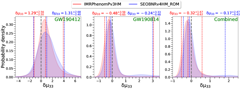
Figure 3: The posterior distributions of $\delta\mu_{33}$, the deformation parameter related to the octupolar tail, for GW190412 and GW190814 analyzed with Phenom (in red color) and SEOB (in blue color) waveform approximants are shown. Left-most panel shows the bounds for GW190412, whereas the middle panel shows the result for GW190814. The combined bounds are shown in the rightmost panel. The combined bounds are obtained assuming the same deviation for the two events. The posteriors of $\delta\mu_{33}$ from individual events, and its combined value both show consistency with GR prediction.

V Inferring octupole parameters

Given the LIGO/Virgo data, $d$, we are interested in deriving ${\widetilde{P}}(\delta\mu_{3n}|d,\,\mathcal{H})$, the posterior probability distribution on $\delta\mu_{3n}$, for a flat prior on $\delta\mu_{3n}$ (here $\mathcal{H}$ denotes the hypothesis, which is the parametric model we employ.). Towards this, we use Eqs. (9), (10), and (11), along with the two-dimensional posterior distribution $P(\delta\hat{\phi_{b}},\,\nu|d,\,\mathcal{H})$, for different GW events. For example, to derive ${\widetilde{P}}(\delta\mu_{30}|d,\,\mathcal{H})$ we will use Eq. (9) and $P(\delta\hat{\phi_{2}},\,\nu|d,\,\mathcal{H})$. The probability distribution $P(\delta\hat{\phi_{b}},\,\nu|d,\,\mathcal{H})$ is computed for flat priors on $\delta\hat{\phi_{b}}$ and mass ratio. Therefore in the Bayesian framework the samples of $\delta\mu_{3n}$, derived from $P(\delta\hat{\phi_{b}},\,\nu|d,\,\mathcal{H})$, need to be reweighted to obtain posterior $\widetilde{P}(\delta\mu_{3n}|d,\,\mathcal{H})$ that assume flat priors on $\delta\mu_{3n}$ as

$$\begin{split}\widetilde{P}(\delta\mu_{3n}|d,\,\mathcal{H})=\bigg{[}\int d\nu\,d(\delta\hat{\phi}_{b})P(\delta\mu_{3n}|\delta\hat{\phi_{b}},\,\nu,\,\mathcal{H})\;\\ {\widetilde{P}}(\delta\hat{\phi_{b}},\,\nu|d,\,\,\mathcal{H})\;\bigg{]}\times\frac{{\widetilde{\Pi}}(\delta\mu_{3n}|\mathcal{H})}{\Pi(\delta\mu_{3n}|\mathcal{H})}\,.\end{split}$$ (16)

In the above equation, the tilde denotes flat priors or posteriors derived assuming flat prior on the corresponding parameters. Hence ${\widetilde{\Pi}}(\delta\mu_{3n}|\mathcal{H})$ denotes flat prior on $\delta\mu_{3n}$ and ${\widetilde{P}}(\delta\hat{\phi_{b}},\,\nu|d,\,\mathcal{H})$ denote posterior assuming flat priors on $\delta\hat{\phi_{b}}$ and mass ratio. The prior distribution, ${\widetilde{\Pi}}(\delta\mu_{3n}|\mathcal{H})$, is chosen to be uniform between [-30, 30]. While $P(\delta\mu_{3n}|\delta\hat{\phi_{b}},\,\nu,\,\mathcal{H})$ takes care of the coordinate transformation between $(\delta\hat{\phi_{b}},\,\nu)$ to $\delta\mu_{3n}$ (using Eqs. (9)-(11)), $\Pi(\delta\mu_{3n}|\mathcal{H})$ in the above equation is simply $P(\delta\mu_{3n}|\delta\hat{\phi_{b}},\,\nu,\,\mathcal{H})$ for the flat prior on $\delta\hat{\phi_{b}}$ and mass ratio. A detailed derivation of the above equation is provided in Sec. A.2 of the supplementary material.

As GW190814 and GW190412 are the only two events for which a confident detection of higher modes was possible, we will restrict to these two events for our purposes. We use the parameter estimation samples for $\delta\hat{\phi}_{b}$ and symmetric mass ratio ($\nu$) from the GWTC-3 Data Release [91] for these two events, analyzed with different waveform approximants, and estimate the bounds on the parameters $\delta\mu_{3n}$ following this procedure.

While estimating the posterior probability distribution of $\delta\mu_{30}$, we need to ensure that the values of $\delta\mu_{30}$ obtained from a pair of $(\delta{\hat{\phi}_{2}},\,\nu)$ should be real by imposing the condition (See Eq. (9)),

$$\delta\hat{\phi}_{2}\leq\frac{K_{1}(\nu)}{\phi_{2}^{\rm GR}}.$$ (17)

In order to realize this, we discard those samples of $\delta\mu_{30}$ which do not meet the above condition. If we need to remove relatively large number of samples, that means the event is uninformative. We find that for events except GW190814 and GW190412, majority of the samples do not meet this condition. This simply is a reflection of the fact that we are trying to test deviation in octupole moment when its presence is barely there in the signal.

VI Results and conclusions

The posteriors of the leading and two subleading octupole deformation parameters $\delta\mu_{30}$, $\delta\mu_{32}$, and $\delta\mu_{33}$ for GW190412 and GW190814 obtained by the above-mentioned procedure are shown in Fig. 1, Fig. 2, and Fig. 3, respectively. Among the detected events, GW190814 provides the tightest constraints on all the octupole parameters. This is expected as GW190814 is the most unequal mass binary (mass ratio, $q=0.112^{+0.008}_{-0.009}$) among the GW events in the GWTC-3 and asymmetric systems get stronger contributions from non-quadrupolar moments.

In addition to the individual event analysis in Figs. 1-3, we have also obtained the combined bounds on $\delta\mu_{3n}$ using data from multiple events under the assumption that the same value of $\delta\mu_{3n}$ is shared across all the events. The joint constraints on these parameters are obtained by multiplying the individual likelihoods from the events, GW190412 and GW190814, analyzed with Phenom and SEOB waveforms. In the joint analysis the most tightly constrained parameter is $\delta\mu_{30}$ ($\delta\mu_{30}=-0.11^{+0.20}_{-0.18}$ using Phenom waveform and $\delta\mu_{30}=-0.07^{+0.11}_{-0.12}$ using SEOB at the 90% credible level) and the most weakly constrained parameter is $\delta\mu_{33}$ ($\delta\mu_{33}=-0.32^{+1.67}_{-0.62}$ using Phenom waveform and $\delta\mu_{33}=-0.17^{+2.47}_{-0.43}$ using SEOB at the 90% credible level).

Bounds from the two different kinds of waveform approximants show excellent agreement with each other. On all occasions the posterior distributions on $\delta\mu_{3n}$ are statistically consistent with $\delta\mu_{3n}=0$ within 90% credible interval. The posterior distributions of $\delta\mu_{3n}$ for the individual-event analysis as well as joint analysis are showing full agreement with GR. This is the first reported bound on the different PN pieces in mass type octupole moment of compact binary complementing the previous consistency tests in Refs. [28, 29]. It is interesting that these bounds also confirm the consistency of the octupolar tail radiation with the predictions of GR.

A parametrized multipolar waveform that includes higher order modes (contain these multipole parameters in the amplitude of the waveform) is currently under development [92]. Inclusion of multipole parameters in the amplitude is likely to improve the bounds quoted here and will be followed up in the future. Lastly, it is instructive to ask if the GR violations in the $\delta\hat{\phi}_{b}$ posteriors can be captured by the mapping proposed in this work. This is examined in Fig. 4 (see the texts in the Sec. A.3 of the supplementary material for more details). We find that the derived posteriors on $\delta\mu_{3n}$, through this mapping, will be able to detect deviations in the $\delta\hat{\phi}_{b}$-posteriors from GR.

To conclude, the parametrized multipolar waveforms could play a pivotal role in testing GR with current and next-generation GW detectors. The next-generation GW detectors will observe more diverse classes of compact binaries, thereby allowing us to probe even higher multipoles of compact binaries, and the parametrization introduced here will be crucial in such scenarios.

*

Appendix A Supplemental Materials

A.1 Tracking different PN pieces of the mass type octupole moment

With the parametrization introduced in Eq. (4), the different PN contributions from the mass type radiative octupole moment to the GW flux, and hence to the GW phasing, can be separately kept track of. To derive such a parametrized octupolar GW phasing, we follow the MPM formalism [40] along the lines of Ref. [25, 26]. The parametrized multipolar flux schematically reads as

$$\mathcal{F}=\frac{32}{5}\nu^{2}x^{5}\mu_{2}^{2}\bigg{[}1+\mathcal{F}_{\rm 1PN}\,x+\mathcal{F}_{\rm 1.5PN}\,x^{3/2}+\mathcal{F}_{\rm 2PN}\,x^{2}+\mathcal{F}_{\rm 2.5PN}\,x^{5/2}+\mathcal{O}(x^{3})\bigg{]}\,,$$ (18)

where $x=(GM\omega/c^{3})^{2/3}$ is a PN parameter, $\omega$ the orbital angular frequency of the binary. The leading order contribution from the mass-type octupole moment ($U_{ijk}$) to the GW flux first appears at 1PN:

$${\mathcal{F}}_{\rm 1PN}^{\rm Oct}=\left(\frac{\mu_{30}}{\mu_{2}}\right)^{2}\left[\frac{1367}{1008}-\frac{1367}{252}\nu\right]\,.$$ (19)

Therefore the leading order contribution from $U_{ijk}$ to the GW phasing appears at 1PN and is given by Eq. (IV).

The next PN contribution (i.e., 1PN correction to $U_{ijk}$; note that there is no 0.5PN correction to $U_{ijk}$.) from $U_{ijk}$ to the GW flux makes appearance at 2PN which reads as

$${\mathcal{F}}_{\rm 2PN}^{\rm Oct}=\left[-\frac{1367\,\mu_{30}^{2}}{168\,\mu_{2}^{2}}-\frac{8201\,\mu_{30}\,\mu_{32}}{3024\,\mu_{2}^{2}}+\left(\frac{17771\,\mu_{30}^{2}}{504\,\mu_{2}^{2}}+\frac{1139\,\mu_{30}\,\mu_{32}}{84\,\mu_{2}^{2}}\right)\nu-\left(\frac{1367\,\mu_{30}^{2}}{126\,\mu_{2}^{2}}+\frac{2050\,\mu_{30}\,\mu_{32}}{189\,\mu_{2}^{2}}\right)\nu^{2}\right]\,.$$ (20)

Thus the 1PN correction to the octupole moment first appears at 2PN in the phasing. The 2PN phasing coefficient reads,

$$\phi_{4} =\Bigg{(}\frac{242245}{5292}+\frac{4525}{5292}\nu+\frac{145445}{5292}\nu^{2}+\left(\frac{\mu_{30}}{\mu_{2}}\right)^{2}\Bigg{[}-\frac{772355}{21168}+\frac{580975}{3024}\nu-\frac{977405}{5292}\nu^{2}\Bigg{]}+\left(\frac{\mu_{30}\,\mu_{32}}{\mu_{2}^{2}}\right)\Bigg{[}\frac{41005}{1512}$$

$$\quad-\frac{5695}{42}\nu+\frac{20500}{189}\nu^{2}\Bigg{]}+\left(\frac{\mu_{30}}{\mu_{2}}\right)^{2}\left(\frac{\epsilon_{2}}{\mu_{2}}\right)^{2}\Bigg{[}\frac{6835}{9072}-\frac{6835}{1134}\nu+\frac{6835\nu^{2}}{567}\Bigg{]}+\left(\frac{\mu_{30}}{\mu_{2}}\right)^{4}\Bigg{[}\frac{9343445}{508032}-\frac{9343445}{63504}\nu$$

$$\quad+\frac{9343445}{31752}\nu^{2}\Bigg{]}+\left(\frac{\mu_{4}}{\mu_{2}}\right)^{2}\Bigg{[}-\frac{89650}{3969}+\frac{179300}{1323}\nu-\frac{89650}{441}\nu^{2}\Bigg{]}+\left(\frac{\epsilon_{2}}{\mu_{2}}\right)^{2}\Bigg{[}-\frac{785}{378}+\frac{7115}{756}\nu-\frac{835}{189}\nu^{2}\Bigg{]}$$

$$\quad+\left(\frac{\epsilon_{2}}{\mu_{2}}\right)^{4}\Bigg{[}\frac{5}{648}-\frac{5}{81}\nu+\frac{10}{81}\nu^{2}\Bigg{]}+\left(\frac{\epsilon_{3}}{\mu_{2}}\right)^{2}\Bigg{[}-\frac{50}{63}+\frac{100}{21}\nu-\frac{50}{7}\nu^{2}\Bigg{]}\Bigg{)}\,.$$ (21)

With the assumptions $\mu_{l;l\neq 3}=\epsilon_{l}=1$ and $\mu_{3n^{\prime};n^{\prime}\neq 2}=1$, the 2PN phasing coefficient reduces to,

$$\phi_{4}=\phi_{4}^{\rm GR}+K_{3}(\nu)\,\big{(}\mu_{32}-1\big{)},$$ (22)

where $\phi_{4}^{\rm GR}$ and $K_{3}(\nu)$ are given by Eq. (12) and Eq. (13) respectively. Comparing the above equation with the parametrization, $\phi_{4}\rightarrow\phi_{4}^{\rm GR}(1+\delta\hat{\phi}_{4})$, we have:

$$\delta\hat{\phi}_{4}=\frac{K_{3}(\nu)\,\left(\mu_{32}-1\right)}{\phi_{4}^{\rm GR}}\,.$$ (23)

Further, substituting $\mu_{32}\rightarrow(1+\delta\mu_{32})$ into the above equation we got the following expression for $\delta\mu_{32}$:

$$\delta\mu_{32}=\frac{\delta\hat{\phi}_{4}\,\phi_{4}^{\rm GR}}{K_{3}(\nu)}\,.$$ (24)

The 1.5PN correction to $U_{ijk}$, that is the octupolar tail, first appears at 2.5PN in the GW flux:

$${\mathcal{F}}_{\rm 2.5PN}^{\rm Oct}=\pi\,\left(\frac{\mu_{30}\,\mu_{33}}{\mu_{2}^{2}}\right)\left(\frac{16403}{2016}-\frac{16403}{504}\nu\right)\,.$$ (25)

Hence the tail contribution from $U_{ijk}$ to the GW phase shows up at the 2.5PN-logarithmic term. The 2.5PN logarithmic phasing coefficient reads,

$$\phi_{5l} =\pi\Bigg{(}\frac{12080}{63}-\frac{3680}{21}\nu+\left(\frac{\mu_{30}}{\mu_{2}}\right)^{2}\Bigg{[}-\frac{27340}{189}+\frac{109360}{189}\nu\Bigg{]}+\left(\frac{\mu_{30}\,\mu_{33}}{\mu_{2}^{2}}\right)\Bigg{[}\frac{82015}{756}-\frac{82015}{189}\nu\Bigg{]}$$

$$\quad+\left(\frac{\epsilon_{2}}{\mu_{2}}\right)^{2}\Bigg{[}-\frac{20}{9}+\frac{80}{9}\nu\Bigg{]}\Bigg{)}\,.$$ (26)

Assuming $\mu_{l;l\neq 3}=\epsilon_{l}=1$ and $\mu_{3n^{\prime};n^{\prime}\neq 3}=1$, the 2.5PN phasing coefficient simplifies to,

$$\phi_{5l}=\phi_{5l}^{\rm GR}+K_{4}(\nu)\,\big{(}\mu_{33}-1\big{)},$$ (27)

where $\phi_{5l}^{\rm GR}$ and $K_{4}(\nu)$ are given by Eq. (14) and Eq. (15) respectively. Again comparing the above equation with the parametrization, $\phi_{4}\rightarrow\phi_{4}^{\rm GR}(1+\delta\hat{\phi}_{4})$ and replacing $\mu_{33}$ with $(1+\delta\mu_{33})$, we obtained the following expression for $\delta\mu_{33}$:

$$\delta\mu_{33}=\frac{\delta\hat{\phi}_{5l}\,\phi_{5l}^{\rm GR}}{K_{4}(\nu)}\,.$$ (28)

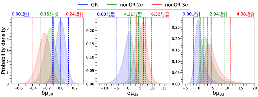
Figure 4: The probability distributions of $\delta\mu_{3n}$ for “GR”, “nonGR 2$\sigma$” and “nonGR 3$\sigma$” cases (see the texts in Sec. A.3 of the supplementary material for more details). The widths of the probability distributions of $\{\nu,\delta\hat{\phi}_{b}\}$ are chosen similar to GW190814. In the “nonGR 2$\sigma$” and “nonGR 3$\sigma$” cases the means of the $\delta\hat{\phi}_{b}$-distributions are 2$\sigma$ and 3$\sigma$ away from zero respectively. The colored vertical dashed lines indicate the 90% confidence intervals and median values. The probability distributions of $\delta\mu_{3n}$ are peaking at zero in the “GR” cases while in the “nonGR 2$\sigma$” and “nonGR 3$\sigma$” cases the distributions of $\delta\mu_{3n}$ are excluding zero at 90% credibility.

A.2 Analysis framework

Within the framework of Bayesian inference, measuring the parameter $\delta\mu_{3n}$ amounts to obtaining the posterior probability density function $P(\delta\mu_{3n}|d,\mathcal{H})$, with $d$ denotes the detector data and $\mathcal{H}$ denotes the model. Using Bayes’ theorem,

$$P(\delta\mu_{3n}|d,\mathcal{H})=\frac{P(\delta\mu_{3n}|\mathcal{H})\,P(d|\delta\mu_{3n},\mathcal{H})}{P(d|\mathcal{H})},$$ (29)

where, $P(\delta\mu_{3n}|\mathcal{H})$ is the prior probability density function, $P(d|\delta\mu_{3n},\mathcal{H})$ is the likelihood function, and $P(d|\mathcal{H})$ (with $P(d|\mathcal{H})=\int d(\delta\mu_{3n})P(\delta\mu_{3n}|\mathcal{H})\,P(d|\delta\mu_{3n},\mathcal{H})$) is the evidence. Here the evidence does not depend on $\delta\mu_{3n}$ and serves as an overall normalization constant. The above equation with uniform prior on $\delta\mu_{3n}$ (i.e., $P(\delta\mu_{3n}|\mathcal{H})={\widetilde{\Pi}}(\delta\mu_{3n}|\mathcal{H})$) can be written as follows,

$$\widetilde{P}(\delta\mu_{3n}|d,\mathcal{H}) =\frac{{\widetilde{\Pi}}(\delta\mu_{3n}|\mathcal{H})\,P(d|\delta\mu_{3n},\mathcal{H})}{P(d|\mathcal{H})}$$

$$=\frac{{\widetilde{\Pi}}(\delta\mu_{3n}|\mathcal{H})\,\int d\nu\,d(\delta\hat{\phi}_{b})\,P(d|\delta\hat{\phi}_{b},\nu,\mathcal{H})\,P(\delta\hat{\phi}_{b},\nu|\delta\mu_{3n},\mathcal{H})}{P(d|\mathcal{H})}$$

$$=\frac{{\widetilde{\Pi}}(\delta\mu_{3n}|\mathcal{H})}{P(d|\mathcal{H})}\,\times\,\int d\nu\,d(\delta\hat{\phi}_{b})P(d|\delta\hat{\phi}_{b},\nu,\mathcal{H})\,\frac{{\widetilde{\Pi}}(\delta\hat{\phi}_{b},\nu|\mathcal{H})\,P(\delta\mu_{3n}|\delta\hat{\phi}_{b},\nu,\mathcal{H})}{\Pi(\delta\mu_{3n}|\mathcal{H})}$$

$$\left(\therefore\Pi(\delta\mu_{3n}|\mathcal{H})\equiv\int d\nu\,d(\delta\hat{\phi}_{b})\,{\widetilde{\Pi}}(\delta\hat{\phi}_{b},\nu|\mathcal{H})\,P(\delta\mu_{3n}|\delta\hat{\phi}_{b},\nu,\mathcal{H})\right)$$

$$={\widetilde{\Pi}}(\delta\mu_{3n}|\mathcal{H})\,\times\,\int d\nu\,d(\delta\hat{\phi}_{b})\bigg{[}\underbrace{\frac{{\widetilde{\Pi}}(\delta\hat{\phi}_{b},\nu|\mathcal{H})\,P(d|\delta\hat{\phi}_{b},\nu,\mathcal{H})}{P(d|\mathcal{H})}}_{\widetilde{P}(\delta\hat{\phi}_{b},\nu|d,\mathcal{H})}\,\times\,\frac{P(\delta\mu_{3n}|\delta\hat{\phi}_{b},\nu,\mathcal{H})}{\Pi(\delta\mu_{3n}|\mathcal{H})}\bigg{]}$$

$$=\bigg{[}\int d\nu\,d(\delta\hat{\phi}_{b})P(\delta\mu_{3n}|\delta\hat{\phi_{b}},\,\nu,\,\mathcal{H})\;{\widetilde{P}}(\delta\hat{\phi_{b}},\,\nu|d,\,\,\mathcal{H})\;\bigg{]}\times\frac{{\widetilde{\Pi}}(\delta\mu_{3n}|\mathcal{H})}{\Pi(\delta\mu_{3n}|\mathcal{H})},$$ (30)

where, ${\widetilde{\Pi}}(\delta\hat{\phi}_{b},\nu|\mathcal{H})$ and $\widetilde{P}(\delta\hat{\phi}_{b},\nu|d,\mathcal{H})$ are the flat prior probability density function and the corresponding posterior probability density function of {$\delta\hat{\phi}_{b},\nu$}, respectively. The probability density function $P(\delta\mu_{3n}|\delta\hat{\phi}_{b},\nu,\mathcal{H})$ maps the posterior samples of {$\delta\hat{\phi}_{b},\nu$} to samples of $\delta\mu_{3n}$ via the relations given by Eq. (9) for $\{\delta\hat{\phi}_{2},\nu\}\rightarrow\{\delta\mu_{30}\}$, Eq. (10) for $\{\delta\hat{\phi}_{4},\nu\}\rightarrow\{\delta\mu_{32}\}$ and Eq. (11) for $\{\delta\hat{\phi}_{5l},\nu\}\rightarrow\{\delta\mu_{33}\}$. Moreover, $\delta\mu_{3n}$ is a function $f_{3n}(\delta\hat{\phi}_{b},\nu)$ of $\delta\hat{\phi}_{b}$ and $\nu$; hence given a value of the pair {$\delta\hat{\phi}_{b},\nu$}, $\delta\mu_{3n}$ is uniquely determined using the relations mentioned above. Therefore, $P(\delta\mu_{3n}|\delta\hat{\phi}_{b},\nu,\mathcal{H})$ becomes delta function:

$$P(\delta\mu_{3n}|\delta\hat{\phi}_{b},\nu,\mathcal{H})=\delta(\delta\mu_{3n}-f_{3n}(\delta\hat{\phi}_{b},\nu))\,.$$ (31)

In practice one needs to take the posterior samples of {$\delta\hat{\phi}_{b},\nu$} for different GW events and to estimate $\delta\mu_{3n}$ for each sample through the relations mentioned above; and then reweight these samples by the probability $\frac{{\widetilde{\Pi}}(\delta\mu_{3n}|\mathcal{H})}{\Pi(\delta\mu_{3n}|\mathcal{H})}$.

A.3 Detecting GR violation

Here we investigate to what extent deviations in the phase deformation coefficients ($\delta\hat{\phi}_{b}$) will be propagated to the probability distributions of the octupole parameters ($\delta\mu_{3n}$) through this mapping. For demonstration, we consider a GW190814-like system. In order to simulate the GR case, we have drawn samples for $\{\nu,\delta\hat{\phi}_{2}\}$ from a bivariate normal distribution with means, $\{0.09,0.0\}$, standard deviations, $\{0.01,0.05\}$, and correlation coefficient, $-0.29$. After generating the samples for $\{\nu,\delta\hat{\phi}_{2}\}$, we estimate the probability distribution of $\delta\mu_{30}$ (shown in the blue curve in the left-most panel of Fig. 4) following the above-mentioned procedure. As expected, we see that the probability distribution of $\delta\mu_{30}$ is sharply peaking at zero (blue curve in the left-most panel of Fig. 4). In the second scenario, which models a 2$\sigma$ violation of GR, we have chosen the mean associated with $\delta\hat{\phi}_{2}$ to be 0.1 (2$\sigma$ deviation from zero i.e., GR value) and kept all other parameters of the bivariate normal distribution at the same values as before. Again we obtain the probability distribution of $\delta\mu_{30}$ (shown in the green curve in the left-most panel of Fig. 4) and find that the distribution of $\delta\mu_{30}$ excludes zero (GR value) at 90% credibility. To simulate another non-GR scenario, a GR violation at 3$\sigma$, we consider the mean of $\delta\hat{\phi}_{2}$ to be 0.15 (3$\sigma$ deviation from zero i.e., GR value) and obtain the probability distribution of $\delta\mu_{30}$ (red curve in the left-most panel of Fig. 4).

We also performed the similar exercises and obtain the probability distributions on $\delta\mu_{32}$ (middle panel of Fig. 4) and $\delta\mu_{33}$ (rightmost panel of Fig. 4). We find that in the “GR” cases the probability distributions of {$\delta\mu_{3n}$} are peaking at zero (or, very close to zero; the median values of the distributions are zero) while in the “nonGR 2$\sigma$” and “nonGR 3$\sigma$” cases the distributions of {$\delta\mu_{3n}$} are excluding zero at 90% credibility. This demonstrates that the proposed mapping is successful in mapping the posteriors of the PN deformations reliably to the posteriors of the corresponding octupole parameters.