Efficient sparsity adaptive changepoint estimation

Abstract

We propose a computationally efficient and sparsity adaptive procedure for estimating changes in unknown subsets of a high-dimensional data sequence. Assuming the data sequence is Gaussian, we prove that the new method successfully estimates the number and locations of changepoints with a given error rate and under minimal conditions, for all sparsities of the changing subset. Our method has computational complexity linear up to logarithmic factors in both the length and number of time series, making it applicable to large data sets. Through extensive numerical studies we show that the new methodology is highly competitive in terms of both estimation accuracy and computational cost. The practical usefulness of the method is illustrated by analysing sensor data from a hydro power plant, and an efficient R implementation is available.

1 Introduction

During the last decades, new technology has made it possible to gather data in larger quantities from an ever wider range of sources. Data can often display non-stationarities in the form of distributional changes over time, leading to incorrect statistical inferences if not accounted for. Inference on changepoints may also be of interest in it self. For instance, Cunen et al. (2020) search for changes in the number of battle deaths in interstate wars between 1816 and 2007, Gao et al. (2020) study monitoring of the temperature of transplant organs, and Tveten et al. (2022) use a changepoint detection algorithm for condition monitoring of a subsea pump.

In this paper, we study the problem of detection and estimation of an unknown number of changes in the mean of high-dimensional data. By detection, we refer to testing for the presence of one or more changepoints in the data. By estimation, we refer to estimation of the location(s) of the changepoint(s). This problem is well understood in the literature for univariate data,. Several computationally efficient algorithms have been proposed during the last decade, including Pruned Exact Linear Time of Killick et al. (2012), Wild Binary Segmentation of Fryzlewicz (2014), Narrowest Over Threshold of Baranowski et al. (2019) and Seeded Binary Segmentation of Kovács et al. (2022). Notably, these methods have been shown to achieve near optimal performance, in a minimax sense, see Wang et al. (2020).

Several methods for the multivariate change in mean problem have also been proposed, although this problem is less studied than the univariate setting. The Inspect method of Wang and Samworth (2018) uses sparse projections of CUSUM statistics and a variant of Wild Binary Segmentation to detect and localize multiple sparse changes in the mean. Cho and Fryzlewicz (2015) propose the Sparsified Binary Segmentation algorithm based on thresholding and aggregating CUSUM statistics over coordinates, in combination with Binary Segmentation. The Double CUSUM method of Cho (2016) uses test statistics based on ordered CUSUMs, in combination with ordinary Binary Segmentation. The SUBSET method of Tickle et al. (2021) uses a penalized likelihood approach, in combination with the Wild Binary Segmentation search procedure.

In this work, we present a novel multiple changepoint estimation algorithm, which we call ESAC (Efficient Sparsity Adaptive Changepoint estimator). The method is designed to detect and estimate the locations of an unknown number of changes in the mean of high-dimensional data sequences. An important feature of ESAC is that the subset of data components that undergo a change need not be known — it can be anything from a single changing component to a small subset to all components. We refer to the size of the changing subset as the sparsity of the change. ESAC comes with strong theoretical guarantees, and is in particular adaptive to all sparsities of changes and all distances between changepoints. Still, the worst-case computational cost of ESAC is linear in the number of observations, $n$, as well as the number of components, $p$, save for logarithmic factors. Via simulations, we demonstrate that ESAC is highly competetive in terms of statistical accuracy and running time.

The novelty of our work is threefold. Our first contribution is to modify a sparsity adaptive test statistic proposed by Liu et al. (2021) to make it suitable for testing for changepoints in a multiple changepoint setup. In particular, our proposed test facilitates control over its family-wise error rate, which is necessary in the multiple changepoint situation. Our second contribution is to propose a novel estimator for the location of a single changepoint. The estimator comes with strong theoretical guarantees, and may be of independent interest. Lastly and most importantly, we combine our proposed test statistic and changepoint estimator into a multiple changepoint estimation algorithm, ESAC, using a slight variant of Seeded Binary Segmentation (Kovács et al., 2022) and Narrowest-over-Threshold (Baranowski et al., 2019) selection of changepoints. ESAC is also efficiently implemented in an R package HDCD (Moen, 2023), available on The Comprehensive R Archive Network (cran.r-project.org). Efficient implementations of Inspect Wang and Samworth (2018) and the method of Pilliat et al. (2023) are also available in the package.

Most similar to ESAC is the multiple changepoint detection procedure of Pilliat et al. (2023) for Gaussian changes in mean. The theoretical guarantees, for instance, are the same for ESAC and the method of Pilliat et al. (2023). Still, there are important distinctions between the two methods, which we highlight here. As opposed to ESAC, the method proposed by Pilliat et al. (2023) is based on their novel ”bottom up” search. Their approach segments the data into disjoint segments chosen as narrow as possible from a predefined grid, where for each interval, a test statistic must have detected a changepoint. To ensure a disjoint segmentation, they merge overlapping segments of equal length whenever a changepoint is detected in both. From this segmentation, changepoint locations are estimated by taking midpoints of the segments. Consequently, Pilliat et al.’s method only requires a test for a changepoint, and not a location estimator. In practice, this generality comes at a cost of changepoints being crudely estimated or not being detected at all, whenever the signal strength is low. This is illustrated in our simulation studies, which feature empirical comparisons between ESAC, the method of Pilliat et al. (2023) and other proposed methods.

The paper is organized as follows. In Section 2 we give a formal description of the model assumed throughout the paper. In Section 3.1 we present a test statistic for a single changepoint that facilitates control over its family-wise error rate. In Section 3.2 we propose an estimator for the location of a single changepoint, also stating its finite sample estimation error rate with comparisons to other methods. In Section 3.3 we propose ESAC, our proposed multiple changepoint estimation procedure. In Section 3.4 we present theoretical results regarding the statistical and computational properties of ESAC and compare these to other methods. In Section 4 we study the empirical performance of ESAC and other methods via simulations, including for misspecified models. In Section 5 we apply ESAC to sensor data from a Swedish hydro power plant. In Appendix A we prove our main theoretical results. In the remained of the Appendix we discuss implemention of ESAC in practice, provide more simulation results, and prove auxiliary lemmas for our main results.

We use the following notation throughout the paper. For any vector $y\in\mathbb{R}^{d}$ we let $y_{j}$ denote its $j$-th component, $\left\lVert y\right\rVert_{2}$ denote its Euclidean norm and $\left\lVert y\right\rVert_{0}$ denote the number of non-zero entries in $y$. For any matrix $X\in\mathbb{R}^{p\times n}$ we let $X_{i,v}$ denote its $(i,v)$th element, $X_{v}\in\mathbb{R}^{p}$ denote its $v$th column, $X_{{}_{i,\bm{\cdot}}}\in\mathbb{R}^{n}$ denote its $i$th row, $\left\lVert X\right\rVert_{F}^{2}=\sum_{i=1}^{p}\sum_{v=1}^{n}X_{i,v}^{2}$ denote the squared Frobenius norm of $X$, and $\left\lVert X\right\rVert_{1}=\sum_{i=1}^{p}\sum_{v=1}^{n}|X_{i,v}|$ denote the entry-wise $\ell_{1}$ norm of $X$. For any pair of matrices $X,Y\in\mathbb{R}^{p\times n}$, we let $\left\langle X,Y\right\rangle=\text{tr}\left(X^{{\mathrm{\scriptscriptstyle T}}}Y\right)$ denote their trace inner product. For any positive integer $I$ we define $[I]=\{1,\ldots,I\}$. For any pair of real numbers $x,y$, we define $x\vee y=\max\left\{x,y\right\}$ and $x\wedge y=\min\left\{x,y\right\}$. For any pair of random variables $X,Y$, we let $X\leq_{\text{st}}Y$ mean that $Y$ stochastically dominates $X$, i.e. $\mathbb{P}\left(X\leq t\right)\geq\mathbb{P}\left(Y\leq t\right)$ for all $t\in\mathbb{R}$. For any $x\in\mathbb{R}$, we let $\lfloor x\rfloor$ denote the largest integer no larger than $x$, and $\lceil x\rceil$ denote the smallest integer no smaller than $x$.

We find it useful to adopt the notation of Baranowski et al. (2019) to denote integer intervals. For any pair of integers $s,e$ such that $s\leq e-2$, we let $(s,e)$ denote the open integer interval $\{s+1,\ldots,e-1\}$ and let $(s,e]$ denote the left-open and right closed integer interval $\{s+1,\ldots,e\}$.

2 Problem description

To motivate our method and allow for theoretical analysis, we consider the following model for the remainder of the paper. In Section 4 we assess performance under various misspecified models. Suppose we observe $n\geq 2$ independent multivariate Gaussian variables

$$X_{v}=\mu_{v}+W_{v},$$ (1)

where $\mu_{v}\in\mathbb{R}^{p}$ and $W_{v}\sim\text{N}_{p}(0,\sigma^{2}I)$ for $v\in[n]$. Assume that there are $J\geq 0$ changepoints $0<\eta_{1}<\ldots<\eta_{J}<n$ such that

$$\mu_{v}\neq\mu_{v+1}\text{ if and only if }v=\eta_{j}\text{ for some }j\in[J].$$

Let $\theta_{j}=\mu_{\eta_{j+1}}-\mu_{\eta_{j}}$ denote the change in mean occurring at the $j$th changepoint, and let $\varphi_{j}=\left\lVert\theta_{j}\right\rVert_{2}$ be the $\ell_{2}$-norm of the mean-change occuring at changepoint $j$. Further, let $k_{j}=\left\lVert\theta_{j}\right\rVert_{0}$ denote the sparsity of the $j$th changepoint, i.e. the number of non-zero components of $\theta_{j}$. Lastly, let $\Delta_{j}=\min\left(\eta_{j}-\eta_{j-1},\eta_{j+1}-\eta_{j}\right)$ denote the minimum distance between the $j$th changepoint and a neighboring changepoint (where we for convenience take $\eta_{0}=0$ and $\eta_{J+1}=n$). Our goal is to estimate $J$, the number of changepoints, and their locations $\eta_{1}<\ldots<\eta_{J}$.

In the theoretical analysis to follow, we take $\sigma^{2}$ to be known. For notational compactness, let $X$, $\mu\in\mathbb{R}^{p\times n}$ denote the matrices with $X_{v}$, $\mu_{v}$ as their $v$th columns, respectively, for $v\in[n]$.

3 Method and results

3.1 Single changepoint detection with family-wise error rate control

We begin by presenting a statistical test for a single change in mean in some arbitrary interval $(s,e)=\{s+1,\ldots,e-1\}$, where $0\leq s<e\leq n$, and $s\leq e-2$. To simplify the exposition, assume for now that $\sigma=1$, as the data can be normalized to satisfy this assumption. We seek a test statistic which facilitates control over the family-wise error rate when testing for changepoints over multiple intervals. This level of control is needed later on when we define a multiple changepoint algorithm in Section 3.3.

To construct a test statistic, we build upon the work of Liu et al. (2021). They propose an efficient and minimax rate optimal test statistic for testing for a single changepoint within an interval. Unfortunately, this test does not allow for control of the family-wise error rate, and thus needs some modifications, presented next. For any candidate changepoint location $v$ such that ${0\leq s<v<e\leq n}$, we define the CUSUM transformation $T^{v}_{(s,e]}(y)$ of a vector $y\in\mathbb{R}^{n}$ as

$$T^{v}_{(s,e]}(y) =\left\{\frac{e-v}{(e-s)(v-s)}\right\}^{1/2}\sum_{i=s+1}^{v}y_{i}-\left\{\frac{v-s}{(e-s)(e-v)}\right\}^{1/2}\sum_{i=v+1}^{e}y_{i},$$ (2)

To simplify notation, we use $C_{(s,e]}^{v}(i)=T^{v}_{(s,e]}(X_{i,\cdot})$ to denote the CUSUM of the $i$th component of the data within the integer interval $(s,e]$, evaluated at candidate changepoint position $v$.

Given a candidate sparsity level $t\in[p]$, and penalizing function $\gamma(t)$, both to be discussed later, define

$$S_{\gamma,(s,e]}^{v}(t)=\sum_{i=1}^{p}\left\{C^{v}_{(s,e]}\left(i\right)^{2}-\nu_{a(t)}\right\}\mathbbm{1}\left\{|C^{v}_{(s,e]}(i)|\geq a(t)\right\}-\gamma(t),$$ (3)

where the threshold value $a(t)$ is given by

$$a^{2}(t)=4\log\left(\frac{ep\log n}{t^{2}}\right)\mathbbm{1}\left\{t\leq(p\log n)^{1/2}\right\},$$ (4)

and $\nu_{a(t)}$ is a mean-centering term defined by taking $\nu_{a}=\mathbbm{E}\left(Z^{2}\ |\ |Z|\geq a\right)$ for $Z\sim\text{N}(0,1)$ and $a\geq 0$. In (4) we abuse notation slightly, writing $e=\exp(1)$ to mean Euler’s number.

We refer to $S_{\gamma,(s,e]}^{v}(t)$ as a sparsity-specific penalized score, which heuristically measures the degree of evidence of a changepoint at $v\in(s,e)$ with sparsity $t$. To see this, we note that the CUSUM is a well known test statistic for a univariate change in mean, rejecting the null hypothesis of a constant mean for large values (see Wang et al., 2020). In the multivariate case, the statistic (3) aggregates CUSUM values in an effort to borrow information across coordinates. To prevent the noise drowning the signal, the CUSUMs are thresholded at level $a(t)$, tailored specifically for a given sparsity level $t$. The functional form of $a(t)$ is depicted in Figure 1 , where one observes that $a(t)$ decreases with $t$. Hence, $S_{\gamma,(s,e]}^{v}(t)$ thresholds CUSUMs less harshly as $t$ grows. More intuition on $a(t)$ is discussed in the end of this subsection. Also plotted in Figure 1 is $\nu_{a(t)}$, which serves as a mean-centering term for spuriously large CUSUMs, and satisfies $a^{2}(t)\leq\nu_{a(t)}\leq a^{2}(t)+2$. Even after thresholding and mean-centering, however, the sum in (3) need not be small even when no changepoint is present. The role of the penalty function $\gamma(t)$ is therefore to ensure that $S^{v}_{\gamma,(s,e]}<0$ with high probability whenever no changepoint is present.

The sparsity-specific penalized score $S_{\gamma,(s,e]}^{v}(t)$ is defined for a fixed sparsity $t$, while the true sparsity of a changepoint is taken to be unknown. To measure the overall degree of evidence of a changepoint at location $v$, we consider an exponentially increasing grid of candidate sparsity levels

$$\mathcal{T}=\{1,2,4,\ldots,2^{\log_{2}\left\{\lfloor\surd(p\log n)\rfloor\right\}}\}\cup\{p\}.$$ (5)

This approach is also taken by Liu et al. (2021), where the grid $\mathcal{T}$ is slightly smaller. This choice of grid is justified as follows. Whenever a changepoint has true sparsity $k<(p\log n)^{1/2}$, there always exists some $t\in\mathcal{T}$ such that $t/2\leq k\leq t$, which turns out to be sufficient for detecting the changepoint. Conversely, when the true sparsity $k$ satisfies $\geq(p\log n)^{1/2}$, it is sufficient to consider $t=p$.

For a candidate changepoint position $s<v<e$, define the penalized score $S^{v}_{\gamma,(s,e]}$ as

$$S^{v}_{\gamma,(s,e]} =\underset{t\in\mathcal{T}}{\max}\ S^{v}_{\gamma,(s,e]}(t),$$ (6)

which heuristically measures the degree of evidence of a changepoint at location $v$, irregardless of the sparsity. As test statistic for a changepoint in the interval $(s,e)$, we take

$$S_{\gamma,(s,e]}=\mathbbm{1}\left\{\underset{s<v<e}{\max}S^{v}_{\gamma,(s,e]}>0\ \right\}.$$ (7)

As for the penalty function $\gamma(t)$, for $t\in[p]$ define

$$r(t)=r(t,n,p) =\begin{cases}(p\log n)^{1/2}&\text{ if }t\geq(p\log n)^{1/2},\\ t\log\left(\frac{ep\log n}{t^{2}}\right)\vee\log n&\text{ otherwise.}\end{cases}$$ (8)

With penalty function $\gamma(t)=\gamma_{0}r(t)$ for some suitably large constant $\gamma_{0}>0$, we obtain the following control over the family-wise error rate.

Proposition 3.1.

Consider the model in Section 2. For all $s,e$ and $v$ such that $0\leq s<v<e\leq n$, assume that the quantity $S_{\gamma,(s,e]}$ is computed with variance-scaled input matrix $\widetilde{X}=({1}/{\sigma})X$ and penalty function $\gamma(t)=\gamma_{0}r(t)$ for some $\gamma_{0}>0$. Let $I$ denote the set of all intervals $(s,e)\subseteq(0,n)$ containing no changepoint, i.e. satisfying $\eta_{j}\notin(s,e)\ \forall j\in[J]$. For any $\varepsilon>0$, there exists a universal choice of $\gamma_{0}>0$ (depending only on $\varepsilon$) such that

$$\mathbb{P}\left(\underset{(s,e)\in I}{\max}\ S_{\gamma,(s,e]}>0\right)\leq\varepsilon.$$

Some remarks are in order. Figure 1 displays plots of $a^{2}(t)$, $\nu_{a(t)}$ and $r(t)$ as functions of $t$, for $n=p=500$. As our first remark, we observe that $a(t)$ and $\nu_{a(t)}$ are decreasing in $t$, while $r(t)$ is increasing for all $t\leq(p\log(n)/e)^{1/2}$, but with a bulk when $t$ is close to $(p\log n)^{1/2}$. Several equivalent monotonic functions can be chosen in the place of $r(t$), but we have chosen $r(t)$ due to its simple analytical form. The function $r(t)$ can be seen as the information theoretic detection boundary in terms of the signal-to-noise (SNR) ratio for multiple changes in mean of sparsity $t$ in $p$-dimensional Gaussian vectors with sample size $n$ (see Section 3.4 or Pilliat et al. 2023). When $p=1$, we recover the standard penalty used in the univariate changepoint literature for Gaussian changes in mean (see e.g. Wang et al. 2020), as $r(1)=\log n$ in this case. As our second remark, the forms of the threshold $a(t)$ and penalty function $\gamma(t)\propto r(t)$ reflect the two sparsity regimes known in the statistical literature on multivariate mean change detection. In the sparse case where $t\leq(p\log n)^{1/2}$, the threshold $a(t)$ is non-zero and satisfies $a^{2}(t)\approx r(t)/t$, which is decreasing with $t$. Meanwhile, in the dense case where $t>(p\log n)^{1/2}$, the threshold satisfies $a(t)=0$, in which case no thresholding takes place and all CUSUMs contribute to (3).

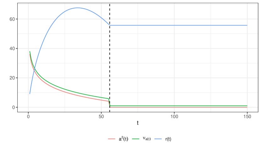
Figure 1: Plots of $a^{2}(t)$ (red), $\nu_{a(t)}$ (green), and $r(t)$ (red) for $n=p=500$. The boundary between the dense and sparse regimes is given by a vertical dashed line at $k=(p\log n)^{1/2}$.

Lastly, we remark the following relation between our proposed test statistic and that of Liu et al. (2021). To facilitate control over the family-wise error rate, the threshold $a(t)$, the mean-centering term $\nu_{a(t)}$, and the penalty function $\gamma(t)=\gamma_{0}r(t)$ grow faster with $n$ than their equivalent counterparts in Liu et al. (2021). To recover the test statistic from Liu et al. (2021), one must replace $\log n$ by $\log\log(8n)$ in (3), (4), (5), (6), (7) and (8) and use the penalty function $\gamma(t)=\gamma_{0}r(t)$ with the modified function $r(t)$.

3.2 Single changepoint estimation

We now consider the problem of estimating the location of a changepoint within some interval $(s,e)$, assuming the changepoint has already been detected or is known to be present. As before, we assume $\sigma=1$, as the data can be normalized to satisfy this assumption. We further assume that the interval $(s,e)$ contains only a single changepoint. Recalling the model defined in Section 1, this means that $J=1$ and $[s,e)=[0,n)$. The problem at hand is then to estimate the location $\eta=\eta_{1}$ of a single changepoint, taking the sparsity $k=k_{1}$ as unknown. As our estimator for $\eta$, we use the test statistic in (6) with a potentially separate penalty function $\lambda(t)$, and maximize it over all candidate changepoints. That is,

$$\widehat{\eta}_{\lambda}=\underset{0<v<n}{\arg\max}\ S^{v}_{\lambda},$$ (9)

where we write $S^{v}_{\lambda}$ shorthand for $S^{v}_{\lambda,(0,n]}$. The rationale behind this estimator is that $S^{v}(\lambda)$ measures the degree of evidence of a changepoint at location $v$. The maximizer is unique with high probability whenever the signal strength is reasonably large. Still, to ensure that $\widehat{\eta}_{\lambda}$ is always well defined, we formally set $\widehat{\eta}_{\lambda}$ be the smallest maximizer, although we suppress this from the notation.

The finite sample properties of $\widehat{\eta}_{\lambda}$ are given in Theorem 3.2, which holds whenever $\lambda(t)=\lambda_{0}r(t)$ for sufficiently large $\lambda_{0}>0$. Before stating the theorem, some remarks are in order. The threshold $a(t)$ is as before decreasing in $t$, while a penalty function of the form $\lambda(t)=\lambda_{0}r(t)$ is increasing for most values of $t$. For such $\lambda(t)$, the penalized score $S^{v}_{\lambda}$ involves an implicit model selection in terms of the sparsity. An inspection of the proof of Theorem 3.2 reveals the following intuition about the roles of $\lambda(t)$ and $a(t)$; whenever $\lambda_{0}$ is sufficiently large, the penalty function $\lambda(t)=\lambda_{0}r(t)$ cancels all contributions to the sum in (3) from coordinates where there is no signal. Left are the contributions from the affected the coordinates. For a changepoint with a moderate signal strength, these remaining contributions are maximized when $t$ is close to the true sparsity $k$. To see this, note that when is $t$ smaller than the true sparsity $k$, the thresholding is too strict, possibly cancelling the signal from the affected coordinates, either from the thresholding itself or from the mean-centering term. When $t$ is greater $k$, the thresholding is less strict, but the penalty function $\lambda(t)$ may be larger than the signal strength from the affected coordinates.

The following finite sample result shows that the estimator $\widehat{\eta}_{\lambda}$ is adaptive to the (unknown) sparsity and gives a high-probability upper bound on the estimation error.

Theorem 3.2.

Consider the model in Section 2, with only one changepoint $\eta$, with sparsity $k$ and $\ell_{2}$ norm $\varphi$. Let $\Delta=\min\left(\eta,n-\eta\right)$. Let $\widehat{\eta}_{\lambda}$ be as in (9), when the sparsity-specific score function $S^{v}_{\lambda}(t)=S^{v}_{\lambda,(0,n]}$ from (3) is computed with variance-scaled input matrix $\widetilde{X}=({1}/{\sigma})X$ and penalty function $\lambda(t)=\lambda_{0}r(t)$, where $\lambda_{0}>0$. Define

$$h(t)=h(t,n,p) =\begin{cases}\left[p\left\{\log n\vee\log\log(ep)\right\}\right]^{1/2}&\text{ if }t\geq(p\log n)^{1/2},\\ t\log\left(\frac{ep\log n}{t^{2}}\right)\vee\log n&\text{ otherwise.}\end{cases}$$ (10)

There exist a universal choice of $\lambda_{0}>0$ and universal constants $C_{0},C_{1}>0$ such that, if

$$\frac{\varphi^{2}\Delta}{\sigma^{2}}\geq C_{0}h(k),$$ (11)

we have that

$$\mathbb{P}\left\{|\widehat{\eta}_{\lambda}-\eta|\leq C_{1}\frac{\sigma^{2}}{\varphi^{2}}h(k)\right\}\geq 1-\frac{1}{n}.$$

The SNR requirement (11) implies that the absolute estimation error of $\widehat{\eta}_{\lambda}$ satisfies $C_{1}h(k){\sigma^{2}}/{\varphi^{2}}\leq C_{0}/C_{1}\Delta<\Delta$ whenever the conditions of the Theorem holds. In particular, in an asymptotic regime where $k$, $p$, $\Delta$ and $\varphi$ vary with $n$, the quantity $|\widehat{\eta}_{\lambda}-\eta|/\Delta$ converges in probability to $0$ as $n\rightarrow\infty$ whenever $({\varphi^{2}\Delta})/\{{\sigma^{2}}h(k)\}$ diverges with $n$. Similarly, if ${\varphi^{2}}/\{{\sigma^{2}}h(k)\}$ diverges with $n$, then $\widehat{\eta}_{\lambda}$ converges in probability to $\eta$ as $n\rightarrow\infty$. Note that Theorem 3.2 requires that the penalty function $\lambda(t)$ has a specific functional form. For practical choices of the penalty function $\lambda(t)$, we refer to Appendix B.

Some performance comparisons with related methods are in order. In comparison with Theorem 3.2, the SNR condition for the Inspect method (Wang and Samworth, 2018) in the single changepoint case is of the form $\varphi^{2}\Delta/\sigma^{2}\geq Cv(k,n,p,\Delta)$ for some $C>0$, where $v(k,n,p,\Delta)=(n/\Delta)k\log\left(p\log n\right)$. Ignoring constants, we see that lthe SNR condition of ESAC is weaker than that of Inspect whenever $k\geq\log n$ and for all values of $k$ whenever $p\geq n/\log n$. Note also that $v(k,n,p,\Delta)$ consists of the factor $n/\Delta$, which is not the case for ESAC. Once the SNR condition for Inspect is satisfied, its error rate is of order $(\sigma^{2}/\varphi^{2})\log\log n$, which is smaller than that of ESAC, and especially so whenever $k$ is large. For the Double CUSUM algorithm of Cho (2016, Section 4) in the single changepoint case where $\sigma=1$, the asymptotic SNR requirement for consistency implies that $\varphi^{2}\Delta/(k\log^{2}n)\rightarrow\infty$. By ”consistency” we mean that $|\widehat{\eta}_{\text{DC}}-\eta|/\Delta$ converges to $0$ in probability, where $\widehat{\eta}_{\text{DC}}$ is the Double CUSUM estimate of $\eta$. The (asymptotic) SNR requirement for the Double CUSUM algorithm is thus larger than that of ESAC by a factor of at least $k\log^{2}(n)/r(k)$, which grows with $k$ and diverges with $n$. Note that theoretical results for the Double CUSUM algorithm only hold whenever $p$ is of the same order as $n^{\omega}$ for some fixed $\omega>0$. For an empirical comparison between the methods in the single changepoint case, we refer to Section 4.1.

The SNR requirement of ESAC grows much more slowly with $k$ than Inspect and the DC algorithm, which implies that ESAC is able to reasonably estimate dense changepoints under much lower signal strength. Figure 2 displays the SNR requirement of ESAC, Inspect and DC as a function of $k$, when $n=p=500$. On the left plot, the SNRs are plotted on linear scale, while on a log scale to the right. The boundary between the dense and sparse regimes is indicated by the vertical dashed line at $k=(p\log n)^{1/2}$. As the SNRs are only defined up to constants, each SNR requirement is normalized to have value $1$ for sparsity $k=1$. For ESAC, the normalized SNR ratio is $h(k)/h(1)$, while it is simply $k$ for Inspect and DC. As we can see, the SNR condition of ESAC grows much more slowly with $k$ than Inspect or DC. We remark that the apparent bulk in the SNR requirement of ESAC is a result of keeping the mathematical expression simple, as remarked in Section 3.1.

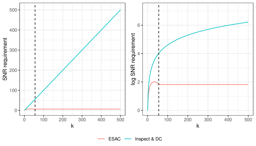
Figure 2: Normalized SNR conditions of ESAC (red) and Inspect and the Double CUSUM algorithm (blue), plotted as a function of the sparsity $k$, on a linear scale (left) and log scale (right). The boundary between the dense and sparse regimes is given by a vertical dashed line at $k=(p\log n)^{1/2}$.

Lastly, we remark the following. For fixed values of $n$ and $p$, the function $h(k)$ is increasing for most values of $k$. Thus, the estimation error and the SNR condition of ESAC tend to grow with the sparsity $k$. As an example, the error rate for estimating a changepoint with sparsity $k=1$ is $(\sigma^{2}/\varphi^{2})\left(\log n\vee\log p\right)$, while the same error rate becomes $(\sigma^{2}/\varphi^{2})\left[p\left\{\log n\vee\log\log(ep)\right\}\right]^{1/2}$ for $k=p$.

3.3 Detection and estimation of multiple changepoints

We now consider the combined problem of detecting and estimating an unknown number of changepoints in the data $X_{1},\ldots,X_{n}$. That is, our goal is to estimate $J$, the number of changepoints, and $(\eta_{1},\ldots,\eta_{J})^{\top}$, the changepoint locations.

Our proposed test statistic from Section 3.1 and changepoint estimator from Section 3.2 are designed for segments with at most a single changepoint. Hence, a search procedure is needed to allow for multiple changepoint search. Our choice of search procedure is a slight variant of Seeded Binary Segmentation (Kovács et al., 2022). In essence, the Seeded Binary Segmentation search procedure generates a deterministic set of intervals (which they call seeded intervals), in which single changepoint candidates are searched for. As a single changepoint may be detected within several distinct intervals, a choice must be made regarding which of these intervals is to be used for estimating its location. We have opted for the Narrowest-Over-Threshold (Baranowski et al., 2019) choice of changepoints, using the narrowest interval in which a changepoint is detected to estimate its location. Our modification of Seeded Binary Segmentation is minor; in our variant, the generation of intervals is controlled by two parameters, $\alpha$ and $K$. The parameter $K$ controls the distance between the centers of two consecutive intervals of the same length, and the parameter $\alpha$ controls the growth rate of the interval lengths. Our algorithm for generating seeded intervals is found in Appendix B (Algorithm 4).

Our proposed multiple changepoint estimation procedure, ESAC, is as follows. Let $\mathcal{M}=\{(s_{m},e_{m}]\ ;\ m\in[M]\}$ denote an enumerated collection of candidate intervals. Let $\gamma(t),\lambda(t)$ denote the penalty functions used in the score statistic (3), for changepoint detection and estimation, respectively. Given data matrix $X$, our proposed procedure is initiated by calling the recursive algorithm ESAC$(X,(0,n],\mathcal{M},\varnothing,\gamma,\lambda)$, defined by Algorithm 1.

For the theoretical analysis of ESAC given in Section 3.4, we find it necessary to consider a slightly modified variant of the algorithm, defined by Algorithm 2 in Appendix B. In this variant, candidate changepoint locations are trimmed away in the recursive step, discarding them from future use to detect or estimate further changepoints. The trimming of changepoints is introduced as a necessary technical step for the proof of Theorem 3.3 to go through, specifically to ensure that previously discovered changepoints are not re-discovered. In practice, we find trimming to be unnecessary and even degrading of performance. An even more modified variant of ESAC, given by Algorithm 3 defined in Appendix B, takes only the midpoint of an interval as the only candidate changepoint location when testing for a changepoint, in addition to interval trimming. This results in a substantial decrease in running time at the cost of reduced detection power, although the theoretical results in the next subsection hold for this variant as well. In practical application, we thus recommend using Algorithm 1 over Algorithms 2 and 3. A simulation study comparing the variants of ESAC is found in Appendix D.

Algorithm 1 ESAC$\left(X,(s,e],\mathcal{M},\mathcal{B},\gamma,\lambda\right)$

Input: A matrix of observations $X\in\mathbb{R}^{p\times n}$, an open integer interval $(s,e)$ in which candidate changepoints are searched for, an enumerated collection $\mathcal{M}=\{(s_{m},e_{m}]\ ;\ m\in[M]\}$ of $M$ half open integer sub intervals of $(0,n]$, a set of already detected changepoints $\mathcal{B}$, and penalty functions $\gamma(t),\lambda(t)$.
Output: Set $\mathcal{B}$ of already detected changepoints.

if $e-s\leq 1$

return $\mathcal{B}$

set $\mathcal{M}_{(s,e]}=\left\{m\in[M]\ :\ (s_{m},e_{m}]\subset(s,e]\right\}$

set $\mathcal{O}_{(s,e]}=\left\{m\in\mathcal{M}_{(s,e]}\ :\ \underset{s_{m}<v<e_{m}}{\max}S^{v}_{\gamma,(s_{m},e_{m}]}>0\right\}$

if $\mathcal{O}_{(s,e]}=\varnothing$

return $\mathcal{B}$

set $l^{*}=\underset{m\in\mathcal{O}_{(s,e]}}{\text{min}}|e_{m}-s_{m}|$

set $\mathcal{O}_{l^{*}}=\left\{m\in\mathcal{O}_{(s,e]}\ :\ |e_{m}-s_{m}|=l^{*}\right\}$

set $m^{*}=\underset{m\in\mathcal{O}_{l^{*}}}{\text{argmax}}\underset{s_{m}<v<e_{m}}{\max}S^{v}_{\lambda,(s_{m},e_{m}]}$

set $v^{*}=\underset{s_{m^{*}}<v<e_{m^{*}}}{\text{argmax}}S^{v}_{\lambda,(s_{m^{*}},e_{m^{*}}]}$

$\mathcal{B}\leftarrow\mathcal{B}\cup\{v^{*}\}$

$\mathcal{B}\leftarrow\text{ESAC}\left(X,(s,v^{*}],\mathcal{M},\mathcal{B},\gamma,\lambda\right)$

$\mathcal{B}\leftarrow\text{ESAC}\left(X,(v^{*},e],\mathcal{M},\mathcal{B},\gamma,\lambda\right)$

return $\mathcal{B}$

3.4 Theoretical results for the multiple changepoint case

For the variants of ESAC defined by either Algorithm 2 or Algorithm 3 (both given in in Appendix B), we have the following finite-sample statistical result.

Theorem 3.3.

Let $X\in\mathbb{R}^{p\times n}$ follow the model in Section 2, and let $r(t)$ be defined as in (8). Let $\mathcal{M}$ denote the set of candidate intervals generated from Algorithm 4 with parameters $\alpha\leq 2$, $K\geq 2$, and let the penalty function $\gamma(t)$ be defined as $\gamma(t)=\gamma_{0}r(t)$. There exists a universal choice of $\gamma_{0}>0$, such that for some universal constants $C_{0},C_{1}>0$, depending only on $\gamma_{0}$, and for any choice of $\lambda(t)$, the following holds.

Let $\widehat{J}$ and $\widehat{\eta}_{1},\ldots,\widehat{\eta}_{\widehat{J}}$ respectively be denote the estimated number of changepoints and sorted changepoint locations from Algorithm 2 or 3, using penalty functions $\gamma(t)$ and $\lambda(t)$, candidate intervals $\mathcal{M}$, and variance scaled input matrix $\widetilde{X}=X/\sigma$. If the SNR condition

$$\frac{\varphi_{j}^{2}\Delta_{j}}{\sigma^{2}}\geq C_{0}r({k}_{j})$$ (12)

holds for all $j\in[J]$, we have that

$$\mathbb{P}\left\{\widehat{J}=J\ \cap\ |\widehat{\eta}_{j}-\eta_{j}|\leq C_{1}\frac{\sigma^{2}}{\varphi_{j}^{2}}r({k}_{j})\ \forall\ j\in[J]\right\}>1-\frac{1}{n}.$$ (13)

The explicit values of $\gamma_{0},C_{0}$ and $C_{1}$ can be found in the proof of Theorem 3.3 in Appendix A. We remark that these constants have not been optimized. In practice, we recommend choosing the penalty functions $\gamma(t)$ via Monte Carlo simulation or setting $\lambda(t),\gamma(t)$ proportional to a slight variant of $r(t)$. In particular, when using $\lambda(t),\gamma(t)\propto r(t)$, our simulations suggest that the leading constants can be chosen independently of $n$ and $p$, at least for the values of $(n,p)$ we have considered. For further details and recommendations, we refer to Appendix B.

Note that, whenever the SNR condition (12) holds, the localization error of ESAC satisfies $C_{1}{\sigma^{2}}r({k}_{j})/{\varphi_{j}}<\Delta_{j}$. If the stronger condition ${\varphi_{j}^{2}}/\{{\sigma^{2}r({k}_{j})}\}\rightarrow\infty$ as $n\rightarrow\infty$ holds for all $j$ (allowing all model parameters to vary with $n$), then ${\max}_{j\in[J]}|\widehat{\eta}_{j}-\eta_{j}|$ converges to $0$ in probability as $n\rightarrow\infty$. Note also that Theorem 3.3 holds for any choice of the penalty function $\lambda(t)$. This is because the bound on the estimation error in Theorem 3.3 relies upon the detection properties of penalized score $S^{v}_{\gamma,(s,e]}$ rather than the localization properties of our estimator $\widehat{\eta}_{\lambda}$. Specifically, since ESAC uses Narrowest-over-Threshold selection of changepoints (Baranowski et al., 2019), it suffices to upper bound the minimum interval width required to detect a changepoint, which for each $j$ is of the order of ${\sigma^{2}}r({k}_{j})/{\varphi_{j}^{2}}$. This observation is due to Pilliat et al. (2023). In practice, we experience that using the estimator $\widehat{\eta}_{\lambda}$ for changepoint localization improves performance compared to using e.g. the mid-point of an interval. For more details and a simulation study, see Appendix D.

Some performance comparisons to related methods are in order. Theorem 3.3 gives a very similar theoretical guarantee as the method of Pilliat et al. (2023, Corollary 3). When the probability of the desired event in the Corollary is the same as in Theorem 3.3, the method of Pilliat obtains the same error rate under an up to constants equal SNR requirement.

The Inspect method (Wang and Samworth 2018) requires a signal-to-noise condition of the form ${\varphi^{2}\Delta}/{\sigma^{2}}\geq C\log(np)\{\left({n}/{\Delta}\right)^{3}\ \vee\ k\}({n}/{\Delta})$, where $C>0$ is some universal constant, $\Delta=\min_{j=1,\ldots,J}\Delta_{j}$, $\varphi=\min_{j=1,\ldots,J}\varphi_{j}$ and $k=\max_{j=1,\ldots,J}k_{j}$. The SNR condition of Inspect is (up to constants) larger than (12) by factors of at least ${n}/{\Delta}\geq 1$ and ${k\log(np)}/{r(k)}\geq 1$. The former factor is only close to $1$ whenever there are few changepoints with large spacing between, while the latter factor is only close to $1$ whenever all changepoints are sparse. For the Double CUSUM algorithm (Cho, 2016) when $\sigma=1$, its (asymptotic) SNR condition requires $\varphi_{j}^{2}\Delta_{j}/(n^{3-5\beta/2}k_{j}\log^{2}n)\rightarrow 0$ whenever $n^{\beta}=\mathcal{O}(\Delta_{j})$ for all $j\in[J]$ for some $\beta\in(6/7,1]$, as well as $p$ being of the same order as $n^{\omega}$ for some fixed $\omega>0$. The SNR requirement for the Double CUSUM algorithm is thus larger than that of ESAC by factors of at least $\surd{n}$ and $k_{j}\log^{2}(n)/r(k_{j})$. The latter factor diverges as $n\rightarrow\infty$ or $k_{j}\rightarrow\infty$.

Figure 3 displays the SNR requirements of ESAC (red), Inspect (green) and the Double CUSUM algorithm (blue) on a log scale as a function of the sparsity $k$, plotted for different values of $n$ and $p$. Here we have removed the factor $\left({n}/{\Delta}\right)^{3}>1$ from the SNR requirement of Inspect, as well as setting $\Delta=n/2$. To the left, we plot the requirements for $n=10^{2},10^{3},10^{4}$, indicated by solid, dashed and dotted lines, respectively, keeping $p=500$ fixed. Moreover, each SNR requirement is normalized to have value $1$ for sparsity $k=1$ at $n=100$. To the right, we plot the requirements for $p=500,1000,2000$, indicated by solid, dashed and dotted lines, respectively, keeping $n=1000$ fixed. Here, each SNR requirement is normalized to have value $1$ for sparsity $k=1$ for $p=500$. From Figure 3 we see that the SNR requirement of ESAC grows substantially slower with $k$ than Inspect and the Double CUSUM. The SNR requirement of ESAC and Inspect grow substantially slower with $n$ than the Double CUSUM, while the SNR requirement of ESAC grows faster with $p$ than Inspect and the Double CUSUM. As before, the apparent bulk in the SNR requirement of ESAC is a result of keeping $r(t)$ mathematically simple, as remarked in Section 3.1.

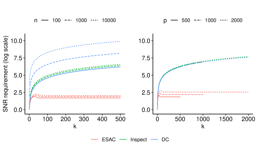
Figure 3: Normalized SNR conditions of ESAC (red) and Inspect (green) and the Double CUSUM algorithm (blue) on a log scale, plotted as a function of the sparsity $k$, and varying values of $n$ (left) and $p$ (right).

As for the changepoint location error rates , Inspect obtains a theoretical error rate of ${\sigma^{2}}({n}/{\Delta})^{4}\log(np)/\varphi^{2}$ whenever its SNR condition is satisfied. In comparison, the theoretical error rate of ESAC is at most ${\sigma^{2}}r(k_{j})/{\varphi_{j}^{2}}r(k_{j})$, which is smaller than the error rate of Inspect whenever ${n}/{\Delta}$ is large (short distance between changepoints) or $k$ is large. For the Double CUSUM algorithm, in the case where $\sigma=1$, the theoretical error rate for each changepoint is at least of the order $\log^{2}(n)k_{j}/\varphi_{j}^{2}$. This is larger than the error rate of ESAC by a factor of at least $k_{j}\log^{2}(n)/r(k_{j})$, which diverges with $n$ and grows with $k_{j}$.

We now turn to optimality considerations. Observe first that the SNR condition (12) is up to constants minimal for identifying $J$, the number of changepoints. Indeed, for any $n$, $p$ and $k\leq p$, an implication of Theorem 2 in Pilliat et al. (2023) is that

$$\sup_{P\in Q(n,p,k)}\ P\left(\left|\widehat{\eta}\right|\neq J\right)\geq 1/4$$

for all estimators $\widehat{\eta}=\widehat{\eta}(X_{1},\ldots,X_{n})$ of the changepoint vector $\eta=(\eta_{1},\ldots,\eta_{J})$, where $Q(n,p,k)$ is the class of all probability distributions of $X_{1},\ldots,X_{n}$ corresponding to the model given in Section 2 for which $k_{j}\leq k$ and $\varphi_{j}^{2}\Delta_{j}/\sigma^{2}\geq cr(k_{j})$ for all $j\in[J]$, for some sufficiently small $c>0$. As for the changepoint location error rate, the minimax rate has been shown by Wang and Samworth (2018) to be at least $\sigma^{2}/(16\varphi^{2})$ whenever $\Delta^{-1}\leq\varphi^{2}/\sigma^{2}\leq 1$. Hence, at least in this region of the parameter space, the estimator $\widehat{\eta}$ from Section 3.2 and the full ESAC algorithm have minimax optimal error rates up to factors of $h(k)$ and $r(k)$, respectively, where $k$ is the sparsity of the changepoint in question. Note that, while $r(k)$ and $h(k)$ are constant multiples of $\log n$ whenever $k=1$, they grow substantially with $k$. Hence the error rate of ESAC is only close to minimax rate optimal for small values of the sparsity $k$.

Finally, we consider the computational cost of ESAC as a function of the size of the data. The following Proposition shows that ESAC has a log-linear computational cost.

Proposition 3.4.

Consider any input matrix $X\in\mathbb{R}^{p\times n}$, penalty functions $\gamma(t),\lambda(t)$ and seeded intervals generated by Algorithm 4 with fixed input parameters $\alpha>1$ and $K\in\mathbb{N}$. Then the computational complexity of ESAC (either Algorithm 1, 2 or 3) measured in floating point operations is of order $\mathcal{O}\left\{np\log(p\log n)\right\}$ in the best case and $\mathcal{O}\left\{np\log n\log(p\log n)\right\}$ in the worst case.

In comparison, the computational complexity of the Pilliat algorithm is $\mathcal{O}\{np\log(np)\}$, which is of slightly smaller order than the worst-case complexity of ESAC. For the other multiple changepoint methods like the Double CUSUM, Sparsified Binary Segmentation, SUBSET and Inspect, no specific forms of computational cost are provided in the respective articles. For an empirical comparison of running times, we refer to the next section.

4 Simulations

We now compare the empirical performance of ESAC with the following state-of-the-art methods for high-dimensional changepoint detection and estimation: a variant of the Inspect method by Wang and Samworth (2018), the method of Pilliat et al. (2023) hereby called Pilliat, Sparsified Binary Segmentation of Cho and Fryzlewicz (2015), the Double CUSUM algorithm of Cho (2016), and the SUBSET method by Tickle et al. (2021). We introduce a slightly modified variant of Inspect, based on Narrowest-over-Threshold search, mainly to reduce computational cost. The details of our modified Inspect algorithm can be found in Appendix C. To run the Sparsified Binary Segmentation and Double CUSUM algorithms, we use the R package hdbinseg (Cho and Fryzlewicz, 2018). To run SUBSET, we use the code from the Github repository of Tickle (2022). We have implemented the remaining methods ESAC, Pilliat and Inspect in the C programming language, which are found in the R package HDCD (Moen, 2023), available on CRAN. We remark that our implementations of Inspect and the method Pilliat et al. are orders of magnitude faster than their original implementations. Whenever running times are reported, they have been run using R (4.2.1) on a MacOS (12.3) computer with an (ARM) Apple M1 Pro CPU.

For each method in the simulation study, a choice of penalty parameters must be made, which is discussed in each subsection. In all simulations, changes in mean are taken to have magnitudes spread evenly across all affected coordinates. In Appendix E we run the same simulations with uneven and random magnitudes, giving similar results. In all simulations we assume $\sigma=1$ is unknown. We estimate $\sigma$ separately for each of the $p$ coordinates of the observed time series, and use it to normalize the data before applying each changepoint detection method. As is commonly done in the changepoint literature, we estimate the noise level by the median absolute deviation of first-order differences with scaling factor 1.05 for the Gaussian distribution.

4.1 Single changepoint estimation

In this subsection we consider the algorithms’ performance when estimating the location of a single changepoint, assuming that it has already been detected. Our simulations are run with parameters $n\in\left\{200,500\right\}$, $p\in\left\{100,1000,5000\right\}$ , $k\in\left\{1,\lceil p^{1/3}\rceil,\lceil\surd{(p\log n)}\rceil,p\right\}$. For each configuration of these parameters, we simulate $1000$ data sets and apply the methods considered in the study. For each combination of $n,p,k$, the simulated data sets have a changepoint at $\eta=\lceil n/5\rceil$ with change-vector $\theta\propto(I_{1},\ldots,I_{k},0,\ldots,0)^{{\mathrm{\scriptscriptstyle T}}}$, where $I_{1},\ldots,I_{k}$ are drawn independently and uniformly from $\{-1,1\}$. For each sample we scale $\theta$ such that $\Delta\varphi^{2}=({n}/{5})\left\lVert\theta\right\rVert_{2}^{2}=({5^{2}}/{2^{2}})r(k)$, where $k$ is the sparsity of the change and $\Delta=\lceil n/5\rceil$.

To keep the simulation study simple, we use the authors’ recommended non-empirical choices of penalty parameters. We take ESAC to be the estimator given in (9), with penalty function $\widetilde{\lambda}(t)$ as defined in Appendix B. As for Inspect, we use Algorithm 2 in Wang and Samworth (2018), with penalty parameter $\lambda=\left\{{\log\left(p\log n\right)/2}\right\}^{1/2}$. For the Double CUSUM algorithm we set $\varphi=-1$, corresponding to the version presented in Section 4.1 of Cho (2016). For Sparsified Binary Segmentation, a default choice of the threshold $\pi_{T}$ is not available, so we take $\pi_{T}$ to be the maximum value of the CUSUMs $|T_{[0,n)}^{v}(Z_{i,\bm{\cdot}}/\widehat{\sigma}_{i})|$ over all values of $0<v<n$ and $i\in[p]$, where $Z_{v,i}{\sim}\text{N}(0,1)$ independently for $i\in[p]$, $v\in[n]$, and $\widehat{\sigma}_{i}$ is the median absolute deviation of the noise level in the $i$th series, based on $1000$ Monte Carlo samples. Whenever the Sparsified Binary Segmentation estimator is not defined, we set its output to be $1$. For both the Double CUSUM and Sparsified Binary Segmentation algorithm, we have specified $\textit{height}=1$ when calling the respective functions to turn the methods into single changepoint estimators. The Pilliat algorithm is not included in this simulation as there is no straightforward way to modify it into a single changepoint estimator.

For each method and each configuration of parameters, Table 1 displays the average Mean Squared Error (MSE) and average running time in milliseconds. The Double CUSUM and Sparsified Binary Segmentation methods are abbreviated as DC and SBS, respectively. For each configuration of parameters, the minimum value of both the MSE and the running is indicated in boldface. In terms of statistical accuracy, Table 1 demonstrates that ESAC and SUBSET are the only methods with competitive accuracy across the sparsity regimes, although ESAC has a slight edge over SUBSET. ESAC has the lowest MSE in $14$ out of the $24$ different combinations of parameters (including both dense and sparse regimes), while SUBSET has the lowest MSE in $6$ out of $24$. When averaging the MSE over all the rows, ESAC is the clear winner, with SUBSET in second place. In comparison, the estimation accuracy of Inspect is excellent for $k=\lceil p^{1/3}\rceil$, but deteriorates for higher sparsity levels. The Double CUSUM algorithm displays excellent estimation accuracy when $k=1$, but often not so for dense changepoints (although this seems to vary slightly with $n$ and $p$). Sparsified Binary Segmentation has high estimation accuracy for sparse changepoints (especially when $k=1$), but the accuracy deteriorates for dense changepoints.

In terms of running time, ESAC is the clear winner, with execution time around one fifth of SUBSET, the runner up, and down to $4\%$ of the execution time of Inspect and Double CUSUM for large values of $p$. Note that SUBSET is the only method not implemented in C or C++, giving the other methods an advantage when comparing running times. We also remark that the running time of scaling the data by the median absolute deviations is not included in the running times of ESAC, Inspect and SUBSET, as it would otherwise dominate the running time. The running time of the scaling is included in the running times of the Double CUSUM and Sparsified Binary Segmentation algorithms, as the implementations of these algorithms do not offer an option to disable it.

Table 1: Single changepoint estimation

Parameters MSE Time in milliseconds $n$ $p$ $k$ $\eta$ $\varphi$ ESAC Inspect SBS SUBSET DC ESAC Inspect SBS SUBSET DC  200 100 1 40 1.40 10.4 25.3 83.0 54.2 9.8 0.4 2.1 9.7 1.7 12.9 200 100 5 40 2.00 5.8 4.1 389.0 3.0 15.3 0.3 2.0 10.4 1.9 13.0 200 100 24 40 1.90 96.5 139.6 1495.8 251.1 953.4 0.2 2.0 9.0 1.6 14.7 200 100 100 40 1.90 95.1 425.9 1520.6 250.8 2807.6 0.2 2.0 9.1 1.6 11.7 200 1000 1 40 1.52 6.9 105.8 29.5 33.1 6.5 2.0 40.8 84.5 12.0 120.6 200 1000 10 40 2.93 5.1 0.8 130.6 1.2 10.4 1.9 40.8 84.0 12.6 122.2 200 1000 73 40 3.37 4.6 64.5 1478.2 8.2 276.1 1.9 40.9 83.4 12.1 122.4 200 1000 1000 40 3.37 3.5 796.2 1534.7 7.1 317.2 2.0 41.0 82.9 12.6 122.2 200 5000 1 40 1.60 45.3 413.3 29.1 81.4 154.2 11.7 210.4 427.9 73.8 651.7 200 5000 18 40 4.00 9.4 0.6 65.7 3.3 94.7 11.6 210.0 426.1 74.3 652.4 200 5000 163 40 5.04 3.6 60.3 1466.2 3.6 7.2 11.8 210.1 422.3 75.0 654.0 200 5000 5000 40 5.04 4.4 1453.9 1563.1 4.4 5.3 11.9 210.1 420.8 75.3 655.4 500 100 1 100 0.92 55.4 97.9 120.8 216.4 54.6 0.7 5.4 16.2 3.9 26.3 500 100 5 100 1.31 22.9 15.7 1060.2 12.6 108.0 0.6 5.3 15.5 3.7 24.9 500 100 25 100 1.25 112.7 323.1 9560.3 2150.5 6850.1 0.6 5.3 16.0 3.6 25.3 500 100 100 100 1.25 284.4 1845.9 9768.9 1959.7 18386.6 0.6 5.2 16.4 3.7 24.3 500 1000 1 100 1.00 30.5 217.7 79.3 190.5 31.0 5.2 252.6 141.9 32.1 256.9 500 1000 10 100 1.90 12.3 5.1 232.6 3.7 84.3 5.4 252.2 142.4 31.7 256.1 500 1000 79 100 2.22 22.1 122.5 9547.8 66.4 1725.7 5.6 253.2 141.6 32.3 256.2 500 1000 1000 100 2.22 15.4 3895.9 9790.4 82.9 2401.7 5.7 254.8 142.6 32.3 258.2 500 5000 1 100 1.05 22.2 1322.6 51.6 95.9 192.0 31.0 1307.0 743.7 168.9 1536.6 500 5000 18 100 2.58 7.9 1.8 102.9 3.2 505.5 30.1 1302.7 726.1 163.7 1434.2 500 5000 177 100 3.32 11.2 175.0 9438.2 11.2 37.6 30.8 1300.5 720.1 158.6 1420.4 500 5000 5000 100 3.32 20.2 8212.5 9799.4 33.7 27.2 31.0 1301.1 717.8 158.3 1415.7 Average MSE 37.8 821.9 2889.1 230.3 1460.9

4.2 Multiple changepoint estimation

In this subsection we consider the situation of an unknown number of changepoints. Our simulations are run with parameters $n=200$, $p\in\left\{100,1000,5000\right\}$ and $J\in\left\{0,2,5\right\}$. For each simulated data set we take the changepoint locations $\eta_{1},\ldots,\eta_{J}$ to be ordered and uniformly drawn samples from $\left\{1,\ldots,n-1\right\}$ without replacement. For each combination of $n,p$ and $J$, we consider three different sparsity regimes; dense, sparse and mixed. In the dense and sparse regimes, we sample $k_{1},\ldots,k_{J}$ independently and uniformly from $\left\{\lceil\surd{(p\log n)}\rceil,\ldots,p\right\}$ and $\left\{1,\ldots,\lfloor\surd{(p\log n)}\rfloor\right\}$, respectively. In the mixed regime we sample each $k_{j}$ independently from a mixture between the dense and sparse regimes, each with equal probability. For each combination of $n,p,J$ and sparsity regime, each changepoint has change-vector $\theta_{j}\propto(I_{j,1},\ldots,I_{j,k},0,\ldots,0){\mathrm{\scriptscriptstyle T}}$, where $I_{j,1},\ldots,I_{j,k}$ are drawn independently and uniformly from $\{-1,1\}$, scaled such that $\Delta_{j}\varphi_{j}^{2}/{\sigma_{j}^{2}}=(7/2)^{2}r(k_{j})$. Notice that we have increased the signal strength slightly in comparison with the single changepoint case, as multiple changepoint estimation is more challenging than estimating the position of a single changepoint whose existence is known. For each combination of $n,p,J$ and sparsity regime we simulate $1000$ data sets.

For both ESAC and the modified Inspect algorithm, we generate seeded intervals using Algorithm 4 with parameters $\alpha=3/2$ and $K=4$. For the Pilliat method we generate intervals using Algorithm 4 with parameters $\alpha=3/2$ and $K=2$, giving very similar intervals as the $a$-adic grid $\mathcal{G}_{a}$ defined in Pilliat et al. (2023) for $a=2/3$. Due to high computational cost, we run SUBSET with only $100$ randomly drawn intervals in its Wild Binary Segmentation step. To ensure comparability with the remaining methods, we have modified the Pilliat algorithm so that its tests for a changepoint in an integer interval $(s,e]$ are performed by testing for a changepoint at each candidate position $s<v<e$, instead of only the mid-point. In our experience, testing only at the mid-point of an interval results in lower detection power.

We choose detection thresholds using either Monte Carlo simulations (using $N=1000$ samples) or bootstrapping (using $B=100$ samples). For the ESAC algorithm, we use the penalty functions $\widetilde{\gamma}(t)$ and $\widetilde{\lambda}(t)$ given in Appendix B, using a false positive rate $\varepsilon=1/N$ to generate the former. For the Pilliat algorithm we choose detection thresholds for the Partial Sum statistic and the dense statistic by Monte Carlo simulating the leading constant in the theoretical thresholds given in Pilliat et al. (2023), and apply a Bonferroni correction. For the modified version of Inspect we set $\lambda=\left\{{\log(p\log n)/2}\right\}^{1/2}$ and choose the detection threshold $\xi$ to be the largest sparse projection over all seeded intervals and over $N=1000$ data sets with no changepoints. For SUBSET we use the function for choosing thresholds provided by the author, which is based on Monte Carlo simulation. For Sparsified Binary Segmentation and Double CUSUM we use the default parameters when running the algorithms (except for setting $\varphi=-1$ for the Double CUSUM algorithm), and use the default bootstrap procedures to select detection thresholds.

For each method considered and each configuration of parameters and changepoint regimes, Table 2 displays the average Hausdorff distance and average absolute estimation error of $J$. The Double CUSUM and Sparsified Binary Segmentation methods are abbreviated as DC and SBS, respectively. For each configuration of parameters and changepoint regimes, the minimum value of each of the performance measures is indicated in boldface. In terms of average Hausdorff distance, Table 2 demonstrates that ESAC and SUBSET are the top performers across all sparsity regimes with comparable accuracy. SUBSET slightly outperforms ESAC when there are few changepoints ($J=2$), while the opposite is true when there are $J=5$ changepoints. Averaging the Hausdorff distance over all configurations, SUBSET is seen to slightly outperform ESAC. We believe this is due to ESAC using Narrowest-Over-Threshold choice of changepoints, which usually causes ESAC to use fewer observations to estimate changepoint locations. See Appendix D for a simulation where ESAC does not use Narrowest-Over-Threshold choice of changepoints locations, improving its performance. For estimating $J$, the number of changepoints, ESAC is the clear winner, with SUBSET in second place.

Figure 4 displays the natural logarithm of the running times (in milliseconds) of the methods as functions of $n$ and $p$. For the left plot, we fix $p=100$, and for the right plot we fix $n=100$. When it comes to execution time, ESAC outperforms the competing methods by a significant margin for all considered values of $n$ and $p$. The running time of ESAC is smaller than that of the competitors by a factor seemingly constant in $n$ and $p$. When not applying a log transform to the running times (which is omitted for brevity), all methods are seen to have an approximately linear computational cost in both $n$ and $p$.

Table 2: Multiple change-point estimation

Parameters Hausdorff distance $\left|\widehat{J}-J\right|$ $n$ $p$ Sparsity J ESAC Pilliat Inspect SBS SUBSET DC ESAC Pilliat Inspect SBS SUBSET DC 200 100 - 0 - - - - - - 0.00 0.00 0.00 0.04 0.00 0.04 200 100 Dense 2 5.27 23.05 21.61 69.92 6.52 76.37 0.06 0.48 0.29 1.03 0.11 1.08 200 100 Sparse 2 1.43 12.54 7.92 49.19 1.67 14.92 0.01 0.25 0.10 0.70 0.04 0.26 200 100 Mixed 2 4.60 18.57 14.36 61.15 3.74 52.93 0.05 0.37 0.19 0.87 0.06 0.74 200 100 Dense 5 5.17 23.74 16.27 67.29 6.42 55.71 0.14 1.53 0.54 3.12 0.33 2.76 200 100 Sparse 5 1.36 13.99 6.38 57.18 2.42 23.19 0.02 0.78 0.23 2.79 0.20 1.36 200 100 Mixed 5 4.04 18.77 12.56 60.43 4.90 41.31 0.10 1.20 0.42 3.01 0.28 2.16 200 1000 - 0 - - - - - - 0.00 0.00 0.00 0.34 0.02 0.02 200 1000 Dense 2 1.45 13.39 9.49 55.12 1.08 84.98 0.01 0.28 0.12 0.72 0.03 1.23 200 1000 Sparse 2 0.83 9.07 9.83 49.72 0.75 20.38 0.00 0.18 0.15 0.62 0.03 0.29 200 1000 Mixed 2 1.78 11.78 9.59 50.51 1.48 53.23 0.01 0.24 0.13 0.69 0.04 0.82 200 1000 Dense 5 1.52 15.81 9.33 57.33 1.56 60.79 0.03 1.02 0.26 2.96 0.17 3.06 200 1000 Sparse 5 0.69 11.34 9.16 54.20 1.52 25.80 0.00 0.64 0.36 2.68 0.17 1.43 200 1000 Mixed 5 1.19 13.93 9.45 58.26 1.72 45.16 0.02 0.81 0.33 2.86 0.19 2.38 200 5000 - 0 - - - - - - 0.00 0.00 0.00 1.96 0.00 0.00 200 5000 Dense 2 0.97 12.99 13.25 54.75 0.60 124.34 0.00 0.29 0.17 0.53 0.02 1.68 200 5000 Sparse 2 0.76 9.66 15.81 58.96 0.51 70.83 0.00 0.20 0.24 0.56 0.03 1.04 200 5000 Mixed 2 0.98 11.36 13.76 55.92 0.78 96.95 0.00 0.25 0.21 0.50 0.03 1.36 200 5000 Dense 5 0.89 14.59 12.97 50.33 1.37 83.64 0.01 0.94 0.45 2.45 0.17 3.63 200 5000 Sparse 5 0.53 11.70 13.50 54.00 1.29 54.33 0.00 0.74 0.55 2.53 0.18 2.71 200 5000 Mixed 5 0.78 13.57 13.25 53.72 1.41 69.94 0.00 0.86 0.50 2.50 0.17 3.19 Average 1.90 14.43 12.13 56.55 2.21 58.60 0.02 0.61 0.29 1.73 0.12 1.73

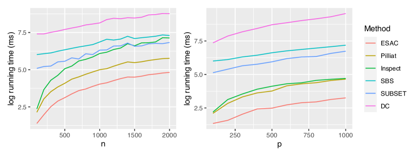
Figure 4: Running times as functions of $n$ (left) and $p$ (right) on a logarithmic scale.

4.3 Misspecified model

ESAC is designed for data with isotropic Gaussian noise, which can be an unrealistic assumption in practice. We now investigate the empirical performance of ESAC and the competing methods in the single changepoint setting under other data generating mechanism than the model described in Section 2. With the changepoint location fixed at $\eta=\lceil n/5\rceil=40$, we consider two sparsity regimes, sparse and dense. We sample $k$ independently and uniformly from $\left\{1,\ldots,\lfloor\surd{(p\log n)}\rfloor\right\}$ in the sparse regime, and from $\left\{\lceil\surd{(p\log n)}\rceil\ldots,p\right\}$ in the dense regime. In both regimes, we take the change-vector $\theta$ to satisfy $\theta\propto(I_{1},\ldots,I_{k},0,\ldots,0)^{{\mathrm{\scriptscriptstyle T}}}$, where $I_{1},\ldots,I_{k}$ are drawn independently and uniformly from $\{-1,1\}$. Furthermore, we scale $\theta$ such that $\Delta\varphi^{2}=({n}/{5})\left\lVert\theta\right\rVert_{2}^{2}=9r(k)$.

Similar to the simulation study in Wang and Samworth (2018), we consider the following data generating mechanisms. In model $M_{0}$ we take the noise vector $W_{v}$ to satisfy $W_{v}\sim\text{N}_{p}(0,I)$ independently for $v\in[n]$. In models $M_{\text{Unif}}$ and $M_{\text{t}_{\text{d}}}$ we take $W_{i,v}\sim\text{Unif}(-\surd{3},\surd{3})$ and $\{d/(d-2)\}^{1/2}W_{i,v}\sim t_{d}$, respectively and independently for all $v\in[n]$ and $i\in[p]$, where $t_{d}$ denotes the Student t distribution with $d$ degrees of freedom. In model $M_{\text{cs, loc}}(\rho)$ we let the noise vectors $W_{1},\ldots,W_{n}$ have short-ranged spatial correlation, taking $W_{v}\sim\text{N}_{p}\left(0,\Sigma(\rho)\right)$ independently for all $v\in[n]$, where $\Sigma(\rho)_{j,k}=\rho^{|j-k|}$ for each $j,k\in[p]$. In the model $M_{\text{cs}}(\rho)$ we let the noise vectors $W_{1},\ldots,W_{n}$ have global spatial correlation by taking $W_{v}\sim\text{N}_{p}\left(0,\Delta(\rho)\right)$ independently for $v\in[n]$, where $\Delta(\rho)=(1-\rho)I_{p}+\rho/pI_{p}I_{p}^{{\mathrm{\scriptscriptstyle T}}}$. In the model $M_{\text{temp}}(\rho)$ we allow for temporal dependence between the noise vectors $W_{1},\ldots,W_{n}$ by letting $W_{1}=\widetilde{W}_{1}$ and $W_{v}=\surd{\rho}\widetilde{W}_{v}+\surd{(1-\rho)}W_{v-1}$ for $v=2,\ldots,n$, where $\widetilde{W}_{1},\ldots,\widetilde{W}_{n}\sim\text{N}_{p}(0,I_{p})$, independently. In the models $M_{\text{async}}$ and $M_{\text{gradual}}$ we allow for changes in the mean to occur asynchronous and gradual in time, respectively, with noise vectors $W_{v}\sim\text{N}_{p}(0,I_{p})$ independently for $v\in[n]$. In $M_{\text{async}}$, for each changepoint $\eta_{j}$, we randomly shift the position (in time) of the change in mean in the $i$th coordinate, where the shifts are drawn independently from $\text{Unif}(\eta_{j}-\lfloor\Delta_{j}/2\rfloor,\eta_{j}-\lfloor\Delta_{j}/2\rfloor+1,\ldots,\eta_{j}+\lfloor\Delta_{j}/2\rfloor)$. In $M_{\text{gradual}}$, for each changepoint $\eta_{j}$, any change in mean occurs linearly over time, starting at position $\eta_{j}-\lfloor\Delta_{j}/2\rfloor+1$ and ending at position $\eta_{j}+\lfloor\Delta_{j}/2\rfloor+1$. For both the single and multiple changepoint settings, we have set $n=p=200$.

Table 3 displays the MSE of the competing methods using the same running parameters as in Section 4.1, based on $N=1000$ runs. Table 3 indicates that ESAC (along with Inspect and SUBSET) is robust to model deviations in the form of light-tailed noise and short-ranged spatial correlation. With global spatial correlation, however, all methods degrade substantially in performance, with Inspect having a slight edge over the remaining methods. With autocorrelation, the performance of the methods also degrades markedly, with ESAC and SUBSET having a slight edge over the remaining methods. Lastly, ESAC and SUBSET seem to be slightly more robust to asynchronous and gradual occurrence of changepoints than the remaining methods.

Table 3: Single changepoint estimation under misspecified models

Parameters		MSE
Model	Sparsity	ESAC	Inspect	SBS	SUBSET	DC
$M$	Sparse	1.2	1.0	506.1	1.1	26.8
$M$	Dense	1.6	84.5	1507.9	1.6	1101.2
$M_{\text{Unif}}$	Sparse	1.0	1.2	666.7	0.9	17.7
$M_{\text{Unif}}$	Dense	7.5	141.3	1506.1	23.4	982.4
$M_{t_{3}}$	Sparse	1373.5	405.7	3014.5	1379.4	3342.1
$M_{t_{3}}$	Dense	1561.6	1184.0	12195.2	1642.9	8132.5
$M_{t_{10}}$	Sparse	2.3	1.5	649.5	1.4	64.3
$M_{t_{10}}$	Dense	2.1	54.6	2045.5	2.1	1256.2
$M_{\text{cs, loc}}(\rho=0.1)$	Sparse	1.1	0.7	497.7	1.0	21.6
$M_{\text{cs, loc}}(\rho=0.1)$	Dense	1.9	69.3	1501.3	1.9	1108.3
$M_{\text{cs, loc}}(\rho=0.4)$	Sparse	1.3	1.2	508.0	1.2	17.9
$M_{\text{cs, loc}}(\rho=0.4)$	Dense	2.7	116.6	1505.7	2.7	1347.6
$M_{\text{cs}}(\rho=0.1)$	Sparse	126.7	2.0	524.3	82.2	20.9
$M_{\text{cs}}(\rho=0.1)$	Dense	281.4	114.4	1516.1	281.4	1111.4
$M_{\text{cs}}(\rho=0.4)$	Sparse	4087.5	66.2	540.1	3997.6	50.7
$M_{\text{cs}}(\rho=0.4)$	Dense	5473.6	1296.8	1503.6	5473.6	2072.9
$M_{\text{AR}}(\rho=0.1)$	Sparse	148.0	77.1	194.2	148.0	175.8
$M_{\text{AR}}(\rho=0.1)$	Dense	40.6	461.7	3023.6	40.6	2557.8
$M_{\text{AR}}(\rho=0.4)$	Sparse	979.9	1648.6	1270.0	979.9	2010.2
$M_{\text{AR}}(\rho=0.4)$	Dense	1274.3	1994.0	2552.5	1274.3	4337.5
$M_{\text{async}}$	Sparse	83.1	99.0	603.8	81.2	233.3
$M_{\text{async}}$	Dense	75.8	288.3	1521.7	79.4	1644.7
$M_{\text{grad}}$	Sparse	50.3	54.5	794.5	49.2	223.8
$M_{\text{grad}}$	Dense	67.7	231.3	1524.4	92.2	2002.1
$M_{\text{grad}}$	Dense	67.7	231.3	1524.4	92.2	2002.1

5 Real data example

To illustrate how ESAC can be applied in practice, we examine raw sensor data from a Swedish hydro power plant. The data consists of measurements from 20 sensors taken every minute for 1800 minutes, so that $p=20$ and $n=1800$. The sensors measure the magnitude of movements and vibrations (the latter measured at 1-10 and 10-1000 Hz bands) at various locations along the shaft connecting the turbine and the generator. During the 1800 minutes we consider, the mode of operation changes several times, detailed in Table 4. We take these changes of operation mode as the ground truth regarding the number of changepoints and their locations.

Table 4: Operation modes of the hydro power plant

Time period Operation mode 1 – 529 running 530 – 537 stopping 538 – 1307 off 1308 – 1310 starting 1311 – 2000 running

The data generating mechanism of the data is undeniably in violation of several underlying assumptions of ESAC. Importantly, the data are highly cross-correlated and auto-regressive. Moreover, the measurements in the data set are influenced by contextual variables such as power output, guide vane opening, and other (human controlled) running conditions in a complex manner. This dependence on contextual variables should ideally be modeled carefully, although such modeling is outside the scope of this paper. As a remedy, we instead transform the observed data by right multiplying each observed data point $X_{i}$ by $\widehat{\Sigma}^{-1/2}$. Here, $\widehat{\Sigma}$ is the estimated variance-covariance matrix of $X_{i}$, estimated from an independent data set with 5992 observations, in which running conditions are stable (i.e. with no changes in operation mode). Moreover, we choose the penalty function $\gamma(t)$ empirically as described in Appendix B, using false probability rate $\varepsilon=0.01$ and letting each of the $N=1000$ Monte Carlo samples $X^{(j)}$ have independent entries following a $t_{5}$ distribution. This choice of penalty function ensures that ESAC is rather conservative in declaring changepoints.

The Monte Carlo simulation for generating the penalty function $\lambda(t)$ took 2 minutes and 2 seconds. Applying ESAC to the data took 0.035 seconds, resulting in six estimated changepoints, at locations 531, 533, 974, 1067, 1308, and 1330. Figure 5 displays the 20 transformed sensor measurements over the sampling period, with estimated changepoint locations indicated by red ticks on the x axis. The grey rectangle in the plot indicate the times at which the plant is either starting, stopping, or off. From the Figure, we clearly see that the first, second and fifth and sixth identified changepoint are associated with a change in operation mode of the plant. Interestingly, the other two changepoints, located at time points 974, 1067, are not associated with a change in running conditions. These changepoints are likely declared by ESAC due to the sudden shift in the yellow curves occurring at time 974 and reverting back again at time 1067.

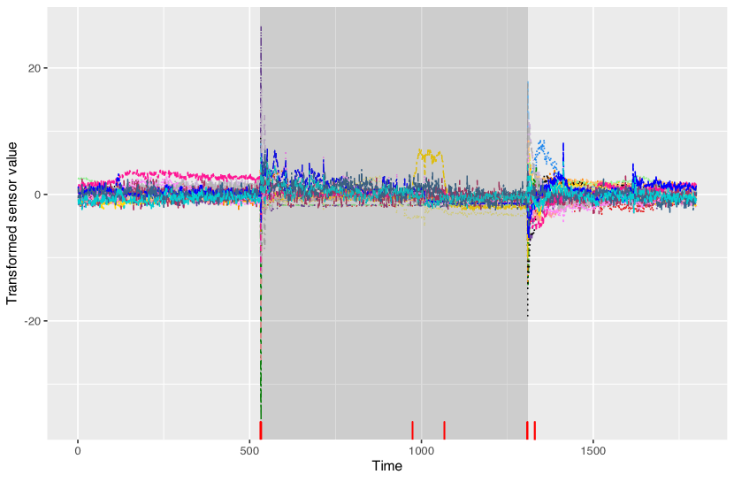
Figure 5: Vibration sensor measurements with detected changepoints indicated by red ticks. Grey areas indicate time intervals in which the plant is starting, stopping or off.

Appendices

A Proofs of main results

Proof of Proposition 3.1.

Set $c_{1}=6+2\log(8/\varepsilon)/\log(2)$, $c_{2}=12+2(\log(1/\varepsilon))^{1/2}+2\log(1/\varepsilon)$ and $\gamma_{0}=9(c_{1}+c_{1}^{1/2}\exp(-1))+c_{2}$. Note first that $I$ has cardinality no larger than $n^{3}$. By a union bound, it thus suffices to show that $\mathbb{P}(S_{\gamma,(s,e]}>0)\leq\varepsilon n^{-3}$ for any $(s,e)\subseteq I$.

So fix any $(s,e)\subseteq I$. Let $t\in\mathcal{T}\setminus\{p\}$ (the case $t=p$ is handled later), and fix $x_{t}>0$ (to be specified shortly). Since $(s,e)$ does not contain any changepoint, we must have ${C}^{v}_{(s,e]}(i)\overset{\text{i.i.d.}}{\sim}\text{N}(0,1)$ for all $i\in[p]$. By Lemma 5.2 we have that

$$\sum_{i=1}^{p}\left\{{C}^{v}_{(s,e]}(i)^{2}-\nu_{a(t)}\right\}\mathbbm{1}{\left\{\left|{C}^{v}_{(s,e]}(i)\right|>a(t)\right\}} \geq 9\left[\left\{pe^{-a(t)^{2}/2}x_{t}\right\}^{1/2}+x_{t}\right]$$ (14)

with probability at most $e^{-x_{t}}$. Now set $x_{t}=c_{1}\left\{\frac{p\log^{2}(n)}{t^{2}}\wedge r(t)\right\}$ for all $t$. Then,

$$\sum_{t\in\mathcal{T}\setminus\{p\}}e^{-x_{t}} \leq\sum_{t\in\mathcal{T}\setminus\{p\}}\exp\left\{-c_{1}\frac{p\log^{2}(n)}{t^{2}}\right\}+\sum_{t\in\mathcal{T}\setminus\{p\}}\exp\left\{-c_{1}r(t)\right\}.$$ (15)

For the first sum, we have

$$\sum_{t\in\mathcal{T}\setminus\{p\}}\exp\left\{-c_{1}\frac{p\log^{2}(n)}{t^{2}}\right\} \leq\sum_{k=0}^{\infty}\exp\left\{-c_{1}{\log(n)}4^{k}\right\}$$ (16)

$$=\sum_{k=0}^{\infty}\left(\frac{1}{n^{c_{1}}}\right)^{4^{k}}$$ (17)

$$\leq n^{-c_{1}}+n^{-c_{1}}\sum_{k=1}^{\infty}\left(\frac{1}{n^{c_{1}}}\right)^{3k}$$ (18)

$$=2n^{-c_{1}}.$$ (19)

For the second sum, noting that $c_{1}r(t)=c_{1}\left\{t\log\left(\frac{ep\log n}{t^{2}}\right)\vee\log n\right\}\geq(c_{1}/2)t\log\left(\frac{ep\log n}{t^{2}}\right)+(c_{1}/2)\log n$, we have

$$\sum_{t\in\mathcal{T}\setminus\{p\}}\exp\left\{-c_{1}r(t)\right\} \leq n^{-c_{1}/2}\exp(-c_{1}/2)\sum_{t\in\mathcal{T}\setminus\{p\}}\left(\frac{t^{2}}{ep\log n}\right)^{c_{1}t/2}$$ (20)

$$\leq n^{-c_{1}/2}\exp(-c_{1}/2)\left(1+\sum_{k=1}^{\infty}4^{-c_{1}t/2}\right)$$ (21)

$$\leq 2n^{-c_{1}/2}.$$ (22)

With this choice of $x_{t}$, we thus have that

$$\sum_{t\in\mathcal{T}\setminus\{p\}}e^{-x_{t}} \leq 4n^{-c_{1}/2},$$ (23)

using that $c_{1}>1$. Moreover, using that $a^{2}(t)=4\log\left(\frac{ep\log n}{t^{2}}\right)$, we have that

$$9\left[\left\{pe^{-a^{2}(t)/2}x_{t}\right\}^{1/2}+x_{t}\right] =9\left[\left\{p\frac{t^{4}}{e^{2}p^{2}\log^{2}n}x_{t}\right\}^{1/2}+x_{t}\right]$$ (24)

$$\leq 9\left\{\frac{tc_{1}^{1/2}}{{e}}+c_{1}r(t)\right\}$$ (25)

$$\leq 9\left(c_{1}^{1/2}\exp(-1)+c_{1}\right)r(t),$$ (26)

where we used that $x_{t}\leq c_{1}r(t)$ and $x_{t}\leq{c_{1}p\log^{2}(n)}/{t^{2}}$, as well as the fact that $t\leq r(t)$ whenever $t\leq(p\log n)^{1/2}$. Recalling that $\gamma(t)=\gamma_{0}r(t)$, since $\gamma_{0}>9\left(c_{1}+c_{1}^{1/2}\exp(-1)\right)$, a union bound gives

$$\ \mathbb{P}\left(\exists t\in\mathcal{T}\setminus\{p\}\ ;\ S_{\gamma,(s,e]}(t)\geq 0\right)$$ (27)

$$= \ \mathbb{P}\left[\exists t\in\mathcal{T}\setminus\{p\}\ ;\ \sum_{i=1}^{p}\left\{{C}^{v}_{(s,e]}(i)^{2}-\nu_{a(t)}\right\}\mathbbm{1}{\left\{|{C}^{v}_{(s,e]}(i)|>a(t)\right\}}\geq\gamma_{0}r(t)\right]$$ (28)

$$\leq 4n^{-c_{1}/2}$$ (29)

$$\leq 4n^{-3-\log(8/\varepsilon)/\log(2)}$$ (30)

$$\leq 4n^{-3}\exp\left(-\log(8/\varepsilon)\log(n)/\log(2)\right)$$ (31)

$$\leq n^{-3}\varepsilon/2,$$ (32)

where we in the last inequality used that $n\geq 2$.

Now consider the case where $t=p$. If $p\leq({p\log n})^{1/2}$, then similarly as above we have that

$$\ \mathbb{P}\left(\ S_{\gamma,(s,e]}(p)\geq 0\right) \leq n^{-3}\varepsilon/2.$$ (33)

If we instead have $p>(p\log n)^{1/2}$ (in which case $a(p)=0$ and $\nu_{a(p)}=1$), then

$$\sum_{i=1}^{p}\left\{{C}^{v}_{(s,e]}(i)^{2}-\nu_{a(p)}\right\}\mathbbm{1}{\left\{|{C}^{v}_{(s,e]}(i)|>a(p)\right\}} =\sum_{i=1}^{p}{C}^{v}_{(s,e]}(i)^{2}-p.$$ (34)

As $\sum_{i=1}^{p}{C}^{v}_{(s,e]}(i)^{2}\sim\chi^{2}_{p}$, we obtain from Lemma 5.4 that

$$\mathbb{P}\left\{\sum_{i=1}^{p}{C}^{v}_{(s,e]}(i)^{2}-p>2(p\log(2n^{3}/\varepsilon))^{1/2}+2\log(2n^{3}/\varepsilon)\right\} \leq n^{-3}\varepsilon/2.$$ (35)

Now,

$$2(p\log(2n^{3}/\varepsilon))^{1/2}+2\log(2n^{3}/\varepsilon) \leq 2(p\log(n^{4}/\varepsilon))^{1/2}+2\log(n^{4}/\varepsilon)$$ (36)

$$\leq 4(p\log n)^{1/2}+2(p\log(1/\varepsilon))^{1/2}+8\log n-2\log(\varepsilon)$$ (37)

$$\leq r(p)\left(12+2(\log(1/\varepsilon))^{1/2}+2\log(1/\varepsilon)\right)$$ (38)

$$=c_{2}r(p)$$ (39)

$$<\gamma_{0}r(p),$$ (40)

using that $n\geq 2$, $r(p)\geq 1$, and $r(p)=(p\log n)^{1/2}\geq\log n$ whenever $p\geq(p\log n)^{1/2}$. Hence,

$$\mathbb{P}\left\{\sum_{i=1}^{p}{C}^{v}_{(s,e]}(i)^{2}-p>\gamma_{0}r(p)\right\} \leq n^{-3}\varepsilon/2.$$ (41)

We conclude that

$$\mathbb{P}\left(\underset{(s,e)\in I}{\max}\ S_{\gamma,(s,e]}>0\right) \leq n^{3}\mathbb{P}\left(\exists t\in\mathcal{T}\ ;\ S_{\gamma,(s,e]}(t)\geq 0\right)$$ (42)

$$\leq n^{3}\left(n^{-3}\varepsilon/2+n^{-3}\varepsilon/2\right)$$ (43)

$$=\varepsilon,$$ (44)

and we are done. ∎

Proof of Theorem 3.2.

Let $\lambda_{0}\geq 63$, $\lambda(t)=\lambda_{0}r(t)$, $C_{1}=2\left\{2\left(4\lambda_{0}+242\right)^{1/2}+2\lambda_{0}+123\right\}$ and $C_{0}>C_{1}$. Let $\widehat{\eta}\in\underset{0<v<n}{\arg\max}\ S^{v}_{\lambda}$, where $S^{v}_{\lambda}$ is defined as in (6), and let $S^{v}(t)$ be defined as in (3). Let the CUSUM transformation $T^{v}_{(s,e]}(\cdot)$ be defined as in (2), and for ease of notation, let $T^{v}(\cdot)=T^{v}_{(0,n]}(\cdot)$ . Let $\mathcal{K}=\left\{i\ ;\ \mu_{i,\eta+1}-\mu_{i,\eta}\neq 0\right\}$ denote the set of coordinates for which there is a change in mean, and for any $0<v<n$ let $\beta_{v}=\sum_{i\in\mathcal{K}}\left\{T^{\eta}(\mu_{i,\bm{\cdot}})^{2}-T^{v}(\mu_{i,\bm{\cdot}})^{2}\right\}$. Let $\overline{k}$ denote the smallest element in $\mathcal{T}$ such that $\overline{k}\geq k$. We may without loss of generality take $\sigma=1$, as we can otherwise normalize the data matrix $X$ and replace the squared norm of the change in mean $\varphi^{2}$ by $\varphi^{2}/\sigma^{2}$.

Consider the event $\mathcal{E}=\mathcal{E}_{1}\cap\mathcal{E}_{2}\cap\mathcal{E}_{3}\cap\mathcal{E}_{4}$ as defined in Lemma 5.5, for which we know that $\mathbb{P}\left(\mathcal{E}\right)\geq 1-\frac{1}{n}$. On the event $\mathcal{E}$, we will show that any $0<v<n$ such that $\left|v-\eta\right|>C_{1}{h(k)}/{\varphi^{2}}$ must satisfy $S^{\eta}_{\lambda}>S^{v}_{\lambda}$, which implies that $\left|\widehat{\eta}_{\lambda}-\eta\right|\leq C_{1}{h(k)}/{\varphi^{2}}$.

Fix some $0<v<n$ and let $t^{*}\in\underset{t\in\mathcal{T}}{\arg\max}\ S^{v}_{\lambda}(t)$, so that $S^{v}_{\lambda}=S^{v}_{\lambda}(t^{*})$. We claim that

$$S^{\eta}_{\lambda}-S^{v}_{\lambda}\geq\beta_{v}-2\left\{{2\beta_{v}h(k)}\right\}^{1/2}-(119+2\lambda_{0})h(k).$$ (45)

To see this, suppose first that $k\leq(p\log n)^{1/2}$. We have that

$$S^{\eta}_{\lambda}-S^{v}_{\lambda} \geq S^{\eta}_{\lambda}(\overline{k})-S^{v}_{\lambda}(t^{*})$$ (46)

$$= \sum_{i=1}^{p}\left[\left({C}^{\eta}(i)^{2}-\nu_{a(\overline{k})}\right)\mathbbm{1}{\left\{\left|{C}^{\eta}(i)\right|>a(\overline{k})\right\}}-\left({C}^{v}(i)^{2}-\nu_{a(t^{*})}\right)\mathbbm{1}{\left\{\left|{C}^{v}(i)\right|>a(t^{*})\right\}}\right]$$

$$-\lambda_{0}r(\overline{k})+\lambda_{0}r(t^{*}).$$ (47)

For any $$x\in\mathbb{R} t\in\mathcal{T} x^{2}-\nu_{a(t)}\leq\left(x^{2}-\nu_{a(t)}\right)\mathbbm{1}{\left\{\left|x\right|>a(t)\right\}}\leq x^{2}$$ and any , we have , and so

$$S^{\eta}_{\lambda}-S^{v}_{\lambda}\geq \sum_{i\in\mathcal{K}}\left[{C}^{\eta}(i)^{2}-{C}^{v}(i)^{2}\right]-k\nu_{a(\overline{k})}$$ (48)

$$+\sum_{i\in[p]\setminus\mathcal{K}}\left[\left({C}^{\eta}(i)^{2}-\nu_{a(\overline{k})}\right)\mathbbm{1}{\left\{\left|{C}^{\eta}(i)\right|>a(\overline{k})\right\}}-\left({C}^{v}(i)^{2}-\nu_{a(t^{*})}\right)\mathbbm{1}{\left\{\left|C^{v}(i)\right|>a(t^{*})\right\}}\right]$$

$$-\lambda_{0}r(\overline{k})+\lambda_{0}r(t^{*}).$$ (49)

On the event $$\mathcal{E}_{1}\cap\mathcal{E}_{2}\cap\mathcal{E}_{3}\supseteq\mathcal{E}$$ we therefore have that

$$S^{\eta}_{\lambda}-S^{v}_{\lambda}\geq \beta_{v}-2\left\{2\beta_{v}\log n\right\}^{1/2}-16r(k)-35r(\overline{k})$$

$$-(63-\lambda_{0})r(t^{*})-\lambda_{0}r(\overline{k})-k\nu_{a(\overline{k})}$$ (50)

$$\geq \beta_{v}-2\left\{2\beta_{v}r(k)\right\}^{1/2}-(92+2\lambda_{0})r(k),$$ (51)

where we have used that $\lambda_{0}\geq 63$, $\log n\leq r(k)$, $r(\overline{k})\leq 2r(k)$, and for $k\leq(p\log n)^{1/2}$, we have $k\nu_{a(\overline{k})}\leq k\left(2+a^{2}(\overline{k})\right)\leq 2k+ka^{2}(k)\leq 6r(k)$. Since $r(k)\leq h(k)$ for all $k\in[p]$, the claim (45) holds whenever $k\leq(p\log n)^{1/2}$.

Now suppose $k>(p\log n)^{1/2}$. By the definition of $\mathcal{E}_{4}$, we have that $S^{v}_{\lambda}(t^{*})-S^{v}_{\lambda}(p)\leq 5h(p)+63r(t^{*})-\lambda_{0}r(t^{*})+\lambda_{0}r(p)$. Hence,

$$S^{\eta}_{\lambda}-S^{v}_{\lambda} \geq S^{\eta}_{\lambda}(p)-S^{v}_{\lambda}(t^{*})$$ (52)

$$=S^{\eta}_{\lambda}(p)-S^{v}_{\lambda}(p)+S^{v}_{\lambda}(p)-S^{v}_{\lambda}(t^{*})$$ (53)

$$\geq S_{\lambda}^{\eta}(p)-S^{v}_{\lambda}(p)-5h(p)-63r(t^{*})+\lambda_{0}r(t^{*})-\lambda_{0}r(p)$$ (54)

$$=\sum_{i=1}^{p}\left\{C^{\eta}(i)^{2}-C^{v}(i)^{2}\right\}-5h(p)-63r(t^{*})+\lambda_{0}r(t^{*})-\lambda_{0}r(p).$$ (55)

On the event $$\mathcal{E}$$ we thus have that

$$S^{\eta}_{\lambda}-S^{v}_{\lambda} \geq\beta_{v}-2\left\{2\beta_{v}\log n\right\}^{1/2}-16r(p)-63r(p)-35r(p)-5h(p)$$ (56)

$$-63r(t^{*})+\lambda_{0}r(t^{*})-\lambda_{0}r(p)$$ (57)

$$\geq\beta_{v}-2\left\{\beta_{v}h(p)\right\}^{1/2}-(119+\lambda_{0})h(p),$$ (58)

where we in the last inequality used that $r(k)\leq h(k)$ for all $k$ and $\lambda_{0}\geq 63$. Hence (45) holds whenever $k>(p\log n)^{1/2}$. Solving the quadratic inequality (45) with respect to $\beta_{v}$, we obtain that $S^{\eta}_{\lambda}-S^{v}_{\lambda}>0$ if

$$\beta_{v}>\left\{2\left(4\lambda_{0}+242\right)^{1/2}+2\lambda_{0}+123\right\}h(k).$$ (59)

Without loss of generality we may assume $v\geq\eta$ (the converse case is similar). By Lemma 5.11 we have that

$$\beta_{v} =\sum_{i\in\mathcal{K}}\left\{T^{\eta}(\mu_{i,\bm{\cdot}})^{2}-T^{v}(\mu_{i,\bm{\cdot}})^{2}\right\}$$ (60)

$$=\frac{|v-\eta|\eta}{|v-\eta|+\eta}\varphi^{2}$$ (61)

$$\geq\frac{1}{2}\min\left(\left|v-\eta\right|\ ,\ \eta\right){\varphi^{2}},$$ (62)

and therefore (59) is satisfied if

$$\min\left(\left|v-\eta\right|\ ,\ \eta\right) >2\left\{2\left(4\lambda_{0}+242\right)^{1/2}+2\lambda_{0}+123\right\}\frac{h(k)}{\varphi^{2}}$$ (63)

$$=C_{1}\frac{h(k)}{\varphi^{2}}.$$ (64)

By the assumption $C_{0}>C_{1}$, $\eta$ is strictly larger than the right hand side of (64). Therefore (59) is satisfied if

$$\left|v-\eta\right| >C_{1}\frac{h(k)}{\varphi^{2}}.$$ (65)

Hence, if $|\eta-v|>C_{1}{h(k)}/{\varphi^{2}}$, we must have $S^{\eta}_{\lambda}>S^{v}_{\lambda}$, and the proof is complete. ∎

Proof of Theorem 3.3.

Let $\gamma_{0}\geq 82$, $\gamma(t)=\gamma_{0}r(t)$ and define $C_{1}=32\left\{\gamma_{0}+170+8\left(2\gamma_{0}+276\right)^{1/2}\right\}$ and $C_{0}=2C_{1}$. We may without loss of generality take $\sigma=1$, as we can otherwise normalize the data matrix $X$ and replace the squared norm of the change in mean $\varphi^{2}$ by $\varphi^{2}/\sigma^{2}$. Let $\mathcal{M}=\{(s_{m},e_{m}]\ ;\ m\in[M]\}$ denote the (enumerated) collection of seeded intervals generated by Algorithm 4. In the following, we will use the name ESAC to refer to either Algorithm 2 or 3. We work on the event $\mathcal{E}=\mathcal{E}_{5}\cap\mathcal{E}_{6}$ as defined in Lemma 5.6, for which we know that $\mathbb{P}(\mathcal{E})\geq 1-1/n$. The proof goes as follows. In step 1 we show that each changepoint $\eta_{j}$ will be detected using a seeded interval with certain properties. In step 2, by an inductive argument, we show that ESAC detects all changepoints within the given error-rate.

Step 1. We first claim that, for each $j$ in $[J]$, there exists a seeded interval $(s_{\widetilde{m}},e_{\widetilde{m}}]=(v-l,v+l]\in\mathcal{M}$ such that the following holds

1. $C_{1}r(k_{j})/(4\varphi^{2}_{j})\leq l\leq C_{1}r(k_{j})/(2\varphi^{2}_{j})\vee 1$;

2. $|\eta_{j}-v|\leq l/2$;

3. $s_{\widetilde{m}}\geq\eta_{j}-(\Delta_{j}/2\vee 1)$;

4. $e_{\widetilde{m}}\leq\eta_{j}+(\Delta_{j}/2\vee 1)$;

5. $S_{\gamma,(s_{\widetilde{m}},e_{\widetilde{m}}]}^{v}\geq 0$.

To see this, fix any $j\in[J]$, and let $h=C_{1}r(k_{j})/(2\varphi^{2}_{j})$. Now let $(s_{\widetilde{m}},e_{\widetilde{m}}]=(v-l,v+l]$ denote the seeded interval from Lemma 5.7. Then properties (P1) and (P2) follow immediately. Moreover, as ${\varphi_{j}^{2}\Delta_{j}}\geq C_{0}r({k}_{j})$ (by the signal-to-noise ratio assumption (12) in Theorem 3.3) and $C_{0}\geq 2C_{1}$, we have $h\leq\Delta_{j}/4$. The properties (P3) and (P4) then follow from Lemma 5.7. To show the last property (P5), observe first that

$$S^{v}_{\gamma,(s_{\widetilde{m}},e_{\widetilde{m}}]}\geq\beta_{(s_{\widetilde{m}},e_{\widetilde{m}}]}^{v}-8\left\{2\beta_{(s_{\widetilde{m}},e_{\widetilde{m}}]}^{v}r(k_{j})\right\}^{1/2}-\left(\gamma_{0}+106\right)r(k_{j}),$$ (66)

on the event $\mathcal{E}$, where $\beta_{(s_{\widetilde{m}},e_{\widetilde{m}}]}^{v}=\sum_{i=1}^{p}T^{v}_{(s_{\widetilde{m}},e_{\widetilde{m}}]}(\mu_{{}_{i,\bm{\cdot}}})^{2}$. By solving the quadratic inequality, we obtain that $S^{v}_{\gamma,(s_{\widetilde{m}},e_{\widetilde{m}}]}\geq 0$ whenever

$$\beta_{(s_{\widetilde{m}},e_{\widetilde{m}}]}^{v} \geq\left\{\gamma_{0}+170+8\left(2\gamma_{0}+276\right)^{1/2}\right\}r(k_{j})$$ (67)

$$=C_{1}/32r(k_{j}).$$ (68)

Assume without loss of generality that $\eta_{j}\leq v$ (the converse case is similar). By the definition of the CUSUM, and using that $|\eta_{j}-v|\leq l/2$, we get that

$$\beta_{(s_{\widetilde{m}},e_{\widetilde{m}}]}^{v} =\frac{v-s_{\widetilde{m}}}{(e_{\widetilde{m}}-s)(e_{\widetilde{m}}-v)}(e_{\widetilde{m}}-\eta_{j})^{2}\varphi_{j}^{2}$$ (69)

$$\geq\frac{1}{2l}(l/2)^{2}\varphi_{j}^{2}$$ (70)

$$=l\varphi^{2}_{j}/8.$$ (71)

Since $l\geq C_{1}r(k_{j})/(4\varphi^{2}_{j})$, we must have that $\beta_{(s_{\widetilde{m}},e_{\widetilde{m}}]}^{v}\geq C_{1}/32r(k_{j})$, which implies (P5).

Step 2. We continue the proof as follows. By induction, with some slight abuse of notation, it suffices to consider any integer interval $(s,e]\subseteq(0,n]$ such that

$$\eta_{h-1}\leq s<\eta_{h}<\ldots<\eta_{h+q}<e\leq\eta_{q+h+1},$$ (72)

for some $q\geq-1$, and, whenever $q>-1$,

$$s \leq\eta_{h}-\Delta_{h}/2;$$ (73)

$$e \geq\eta_{h+q}+\Delta_{h+q}/2.$$ (74)

Note that $q=-1$ corresponds to there being no changepoint in the open integer interval $(s,e)$. We consider this case first. For any seeded interval $(s_{m},e_{m}]\subseteq(s,e]$ and any $s_{m}<v<e_{m}$, we will have that $S^{v}_{\gamma,(s_{m},e_{m}]}<0$, due to the definition of the event $\mathcal{E}$. Hence no changepoint will be declared by ESAC in this case.

Now consider the case where $q>-1$. Note first that a changepoint will be declared by the ESAC algorithm. Indeed, for the $h$th changepoint we may take $(s_{\widetilde{m}},e_{\widetilde{m}}]$ as in step 1, for which the properties (P3) and (P4) imply that $(s_{\widetilde{m}},e_{\widetilde{m}}]\subseteq(s,e]$, due to the inductive hypothesis. By property (P5), we know that $S^{v}_{\gamma,(s_{\widetilde{m}},e_{\widetilde{m}}]}\geq 0$, and hence a changepoint will be detected in $(s,e)$. This implies that $\mathcal{O}_{(s,e]}$, as defined in the ESAC algorithm, satisfies $\mathcal{O}_{(s,e]}\neq\varnothing$. Now let $m^{*}$, $v^{*}$ and $l^{*}$ be as defined in the ESAC algorithm. Note that $(s_{m^{*}},e_{m^{*}})$ must contain a changepoint, say $\eta_{j}$, as we by the definition of $\mathcal{E}$ otherwise would have had $S^{v}_{\gamma,(s_{m^{*}},e_{m^{*}}]}<0$ for any $s_{m^{*}}<v<e_{m^{*}}$. Further, since ESAC uses the narrowest possible seeded interval to estimate a changepoint, we must have that $l^{*}=(e_{m^{*}}-s_{m^{*}})$ satisfies $l^{*}\leq e_{\widetilde{m}}-s_{\widetilde{m}}\leq C_{1}r(k_{j})/(\varphi^{2}_{j})\vee 2$, where $(s_{\widetilde{m}},e_{\widetilde{m}}]$ is the seeded interval as in the claim for $\eta_{j}$. Since $s_{m^{*}}<v^{*}<e_{m^{*}}$, it then follows that

$$|v^{*}-\eta_{j}|\leq\left\{C_{1}r(k_{j})/\varphi^{2}_{j}\vee 2\right\}-2\leq C_{1}\frac{r(k_{j})}{\varphi^{2}_{j}}.$$ (75)

It remains to show that the two new segments in the recursive step, $(s,s_{m^{*}}+1]$ and $(e_{m^{*}}-1,e]$ satisfy the inductive hypothesis. Without loss of generality consider $(s,s_{m^{*}}+1]$ (the argument for the other interval is similar), and suppose that $j\geq h+1$ (otherwise there is nothing to show). To show that the inductive hypothesis holds for $(s,s_{m^{*}}+1]$, it suffices to show that $s_{m^{*}}+1\geq\eta_{j-1}+\Delta_{j-1}/2$. As $\eta_{j}\in(s_{m^{*}},e_{m^{*}})$, we must have $e_{m^{*}}\geq\eta_{j}+1$. Hence

$$s_{m^{*}}+1 =e_{m^{*}}+1-l^{*}$$ (76)

$$\geq\eta_{j}+2-\left\{C_{1}r(k_{j})/\varphi^{2}_{j}\vee 2\right\}$$ (77)

$$=\eta_{j-1}+(\eta_{j}-\eta_{j-1})-\left\{C_{1}r(k_{j})/\varphi^{2}_{j}-2\vee 0\right\}$$ (78)

$$\geq\eta_{j-1}+(\eta_{j}-\eta_{j-1})-\Delta_{j}/2$$ (79)

$$\geq\eta_{j-1}+(\eta_{j}-\eta_{j-1})/2$$ (80)

$$\geq\eta_{j-1}+\Delta_{j-1}/2,$$ (81)

where we in the first inequality used that $l^{*}=(e_{m^{*}}-s_{m^{*}})\leq C_{1}r(k_{j})/\varphi^{2}_{j}\vee 2$ and in the second inequality used that the signal-to-noise ratio condition (12) implies $C_{1}r(k_{j})/\varphi^{2}_{j}\leq\Delta_{j}/2$. Hence the inductive hypothesis holds for $(s,s_{m^{*}}+1]$. ∎

Proof of Proposition 3.4.

Let $\mathcal{M}$ denote the set of seeded intervals generated from Algorithm 4. Note first that computing and storing the cumulative sum of all rows of $X$ requires $\mathcal{O}(np)$ FLOPs. Once these are stored, the number of FLOPs required to compute $C^{v}_{(s,e]}(j)$ as in (2) for some $(s,e]\in\mathcal{M}$ and some $s<v<e$ is of order $\mathcal{O}(p)$. Hence, the number of FLOPs required to compute $S^{v}_{\lambda,(s,e]}$ is of order $p\left|\mathcal{T}\right|=\mathcal{O}\left\{p\log(p\log n)\right\}$. In the best case there are $n-1$ changepoints detected by the ESAC algorithm using all $n-1$ intervals $(s,e]\in\mathcal{M}$ such that $e-s=2$. In this case, the total number of FLOPs executed before ESAC terminates is of order $\mathcal{O}\left\{np+np\log(p\log n)\right\}=\mathcal{O}\left\{np\log(p\log n)\right\}$. In the worst case there are no changepoints detected by ESAC, in which case $S^{v}_{\lambda,(s,e]}$ has to be computed over each triple of integers $s,v,e$ such that $s<v<e$ and $(s,e]\in\mathcal{M}$. By Lemma 5.9, there are at most $\mathcal{O}(n\log n)$ distinct such triples. Hence the number of FLOPs executed before ESAC terminates in this case is of order $\mathcal{O}\left\{np\log n\log(p\log n)\right\}$. ∎

B Implementation details

To apply ESAC in practice, a choice must be made regarding the penalty functions $\lambda,\gamma$, estimation of $\sigma$, as well as the parameters $\alpha$ and $K$ controlling the generation of seeded intervals. In this subsection we discuss these issues in turn, but first, we define two variants of ESAC as well as our algorithm for generating seeded intervals.

B.1 Slight modifications to ESAC

Algorithm 2 constitutes the variant of the ESAC algorithm that features interval trimming. Here, the recursive step in the algorithm (the third and second last lines) differ from those found in 1. When Algorithm 2 declares a changepoint at location $v^{*}$, detected in the interval $(s^{*},e^{*})$, the remaining elements in interval $(s^{*},e^{*})$ are never again used to detect or estimate changepoints.

A faster variant of Algorithm 2 is given by Algorithm 3. Algorithm 3 reduces the execution time by modifying step 3 in Algorithm 2 to only evaluate $S_{\gamma,(s_{m},e_{m}]}^{v}$ at the mid-point $v_{m}=(s_{m}+e_{m})/2$ of any seeded interval. Interestingly, the theoretical guarantees given by Theorem 3.3 also hold for this variant of ESAC, unlike Algorithm 1. Note that the same modification can naturally be made to Algorithm 1 as well. In practice, we have experienced that Algorithm 3 has much lower power for detecting changepoints compared to 1. We therefore only recommend using Algorithm 3 when the consequent reduction in computational cost is necessary.

Algorithm 2 ESAC’$\left(X,(s,e],\mathcal{M},\mathcal{B},\gamma,\lambda\right)$.

Input: Matrix of observations $X\in\mathbb{R}^{p\times n}$, left open and right closed integer interval $(s,e]$ in which candidate changepoints are searched for, an enumerated collection $\mathcal{M}=\{(s_{m},e_{m}]\ ;\ m\in[M]\}$ of $M$ half open integer sub intervals of $\{0,\ldots,n\}$, a set of already detected changepoints $\mathcal{B}$, and penalty functions $\gamma(t),\lambda(t)$.
Output: Set $\mathcal{B}$ of detected changepoints.

if $e-s\leq 1$:

stop

set $\mathcal{M}_{(s,e]}=\left\{m\in[M]\ :\ (s_{m},e_{m}]\subset(s,e]\right\}$

set $\mathcal{O}_{(s,e]}=\left\{m\in\mathcal{M}_{(s,e]}\ :\ \underset{s_{m}<v<e_{m}}{\max}S^{v}_{\gamma,(s_{m},e_{m}]}>0\right\}$

if $\mathcal{O}_{(s,e]}=\varnothing$

stop

set $l^{*}=\underset{m\in\mathcal{O}_{(s,e]}}{\text{min}}|e_{m}-s_{m}|$

set $\mathcal{O}_{l^{*}}=\left\{m\in\mathcal{O}_{(s,e]}\ :\ |e_{m}-s_{m}|=l^{*}\right\}$

set $m^{*}=\underset{m\in\mathcal{O}_{l^{*}}}{\text{argmax}}\underset{s_{m}<v<e_{m}}{\max}S^{v}_{\lambda,(s_{m},e_{m}]}$

set $v^{*}=\underset{s_{m^{*}}<v<e_{m^{*}}}{\text{argmax}}S^{v}_{\lambda,(s_{m^{*}},e_{m^{*}}]}$

$\mathcal{B}\leftarrow\mathcal{B}\cup\{v^{*}\}$

$\mathcal{B}\leftarrow\text{ESAC'}\left(X,(s,s_{m^{*}}+1],\mathcal{M},\mathcal{B},\gamma,\lambda\right)$

$\mathcal{B}\leftarrow\text{ESAC'}\left(X,(e_{m^{*}}-1,e],\mathcal{M},\mathcal{B},\gamma,\lambda\right)$

return $\mathcal{B}$

Algorithm 3 ESAC${{}^{\prime\prime}}\left(X,(s,e],\mathcal{M},\mathcal{B},\gamma,\lambda\right)$

Input: Matrix of observations $X\in\mathbb{R}^{p\times n}$, left open and right closed integer interval $(s,e]$ in which candidate changepoints are searched for, an enumerated collection $\mathcal{M}=\{(s_{m},e_{m}]\ ;\ m\in[M]\}$ of $M$ half open integer sub intervals of $\{0,\ldots,n\}$, a set of already detected changepoints $\mathcal{B}$, and penalty parameters $\gamma,\lambda$.
Output: Set $\mathcal{B}$ of detected changepoints.

if $e-s\leq 1$

stop

set $\mathcal{M}_{(s,e]}=\left\{m\in[M]\ :\ (s_{m},e_{m}]\subset(s,e]\right\}$

set $v_{m}=\left\lfloor\frac{s_{m}+e_{m}}{2}\right\rfloor$ for all $m=1,\ldots,M$

set $\mathcal{O}_{(s,e]}=\left\{m\in\mathcal{M}_{(s,e]}\ :S^{v_{m}}_{\gamma,(s_{m},e_{m}]}>0\right\}$

if $\mathcal{O}_{(s,e]}=\varnothing$

stop

set $l^{*}=\underset{m\in\mathcal{O}_{(s,e]}}{\text{min}}|e_{m}-s_{m}|$

set $\mathcal{O}_{l^{*}}=\left\{m\in\mathcal{O}_{(s,e]}\ :\ |e_{m}-s_{m}|=l^{*}\right\}$

set $m^{*}=\underset{m\in\mathcal{O}_{l^{*}}}{\text{argmax}}\underset{s_{m}<v<e_{m}}{\max}S^{v}_{\lambda,(s_{m},e_{m}]}$

set $v^{*}=\underset{s_{m^{*}}<v<e_{m^{*}}}{\text{argmax}}S^{v}_{\lambda,(s_{m^{*}},e_{m^{*}}]}$

$\mathcal{B}\leftarrow\mathcal{B}\cup\{v^{*}\}$

$\mathcal{B}\leftarrow\text{ESAC}{{}^{\prime\prime}}\left(X,(s,s_{m^{*}}+1],\mathcal{M},\mathcal{B},\gamma,\lambda\right)$

$\mathcal{B}\leftarrow\text{ESAC}{{}^{\prime\prime}}\left(X,(e_{m^{*}}-1,e],\mathcal{M},\mathcal{B},\gamma,\lambda\right)$

return $\mathcal{B}$

B.2 Efficient implementation of ESAC

The ESAC Algorithms 1, 2 and 3 are based on Narrowest-Over-Threshold selection of changepoints. Once a changepoint is detected in some seeded interval, say of length $l^{*}$, the changepoint location is estimated based only on intervals of length $l^{*}$. To minimize running time, any version of ESAC should therefore iterate through the seeded intervals $\left\{(s_{m},e_{m}]\ :\ m\in[M]\right\}$ in the (increasing) order of their width. This computational trick gives significant speed improvements whenever changepoints can be detected by short seeded intervals.

B.3 Choice of $\alpha$ and $K$

The choice of $\alpha$ and $K$ entails a trade-off between computational cost and statistical performance. As either $\alpha^{-1}$ or $K$ increase, more seeded intervals are generated from Algorithm 4, increasing both the chance of detecting a changepoint and the running time of ESAC. After some experimentation, we have experienced that $\alpha=3/2$ and $K=4$ give a decent balance between running time and statistical accuracy.

B.4 Variance re-scaling

In the theoretical analysis of this paper, the noise level $\sigma$ of each time series is assumed known and common across all $p$ time series. In practice, this is an unrealistic assumption. As is common in the changepoint literature, we suggest estimating the noise level separately for each time series by the (scaled) Median Absolute Deviation (MAD) of first-order differences, as in e.g. Wang and Samworth (2018). If it is reasonable to assume that each time series has approximately the same noise level, the common noise level $\sigma$ can be estimated for instance by taking a mean or median of the MAD estimates for each time series. Once estimates of the noise levels are obtained, the time series need only to be re-scaled by their estimated noise levels before applying ESAC.

B.5 Analytical choice of penalty functions

Recall that $\lambda(t)$ and $\gamma(t)$ are the penalty functions used in the penalized score statistic for changepoint localization and detection, respectively. The proofs of Theorems 3.2 and 3.3 provide suggestions for analytical choices of these penalty functions. However, we believe the leading constants are overly conservative. To obtain more practical choices of analytical penalizing functions, we have run simulations for combinations of $n$ up to $1000$ and $p$ up to $5000$. We have experienced that replacing $n$ with $n^{4}$ in $a(t)$ (4) and $r(t)$ (8) gives a slightly better balance between the two terms $t\log\left(\frac{ep\log n}{t^{2}}\right)$ and $\log n$ in $r(t)$. As default values in our R package, as well as in the simulation study, we have replaced $n$ with $n^{4}$ in $a(t)$ and $r(t)$. For changepoint estimation, we recommend using the penalty function

$$\widetilde{\lambda}(t)=\begin{cases}\frac{3}{2}\left\{\left(p\log n^{4}\right)^{1/2}+\log n^{4}\right\}&\text{ if }t\geq(p\log n)^{1/2},\\ t\log\left(\frac{ep\log n^{4}}{t^{2}}\right)+\log n^{4}&\text{ otherwise.}\end{cases}$$ (82)

This recommendation is independent of whether each time series is re-scaled by Median Absolute Deviation (MAD) estimates. The choice of the two leading constants in $\widetilde{\lambda}$ are the result of minimizing the Mean Squared Error (MSE) of the estimator (9) over a rough grid of $n$, $p$, $\eta$ and $k$, where $n$ has ranged from $200$ to $1000$ and $p$ has ranged from $100$ to $5000$. For changepoint detection one can also use $\gamma(t)=\widetilde{\lambda}(t)$, which in our experience gives a false positive rate of less than $1/n$. If the variance of each time series is re-scaled by MAD estimates, however, we recommend choosing the penalty function $\gamma(t)$ for changepoint detection using Monte Carlo simulation.

B.6 Empirical choice of penalty functions

To obtain exact control over the probability of a false changepoint being detected by ESAC, one can choose the penalty function $\gamma(t)$ by Monte Carlo simulation. Consider any false positive probability $\varepsilon>0$ and Monte Carlo sample size $N$. A naive choice of empirical penalty function, denoted by $\widehat{\gamma}_{\varepsilon}(t)$, is given by the following. Let $\mathcal{M}$ denote the collection of seeded intervals to be used by ESAC. Simulate $N$ data sets $\left(X^{(j)}\right)_{j=1}^{N}$ following model (1) with no changepoints, in which each row is re-scaled by MAD estimates if applicable. For each $t\in\mathcal{T}$, let $\widehat{\gamma}_{\varepsilon}(t)$ denote the $\lceil N(1-\varepsilon)\rceil$ largest value of $\underset{(s,e]\in\mathcal{M}}{\max}\ \underset{s<v<e}{\max}\ S_{0,(s,e]}^{v}\left(X^{(j)}\right)(t)$ over $j=1,\ldots,N$, where $S_{0,(s,e]}^{v}\left(X^{(j)}\right)(t)$ is the sparsity-specific score statistic from (3) computed over the seeded interval $(s,e]$ with input matrix $X^{(j)}$ and with penalty function $0$.

Due to multiple testing, the approximate false positive probability when using the naive penalty function $\widehat{\gamma}_{\varepsilon}$ can only be upper bounded by $\left|\mathcal{T}\right|\varepsilon$. To adjust for multiple testing, a Bonferroni correction can easily be applied by replacing $\varepsilon$ by $\varepsilon/\left|\mathcal{T}\right|$ in the definition of $\widehat{\gamma}_{\varepsilon}(t)$. In our experience, though, such a Bonferroni correction is too conservative. An alternative approach to handle the multiple testing is to use the empirical penalty function $\widehat{\gamma}^{*}(t)=r(t)\ \underset{s\in\mathcal{T}}{\max}\ \widehat{\gamma}_{\varepsilon}(s)/r(s)$, in which the functional form is specified and only the leading constant is chosen by Monte Carlo simulation. In our experience, this approach also leads to an overly conservative penalty function, as the functional form of $\widehat{\gamma}_{\varepsilon}(t)$ does not match the theoretical counterpart $r(t)$ exactly. We therefore recommend to use the following penalty function $\widetilde{\gamma}(t)$, in which we introduce three separate leading constants for different segments of $\mathcal{T}$ (and consequently a Bonferroni correction) for slightly more flexibility. Let $\widetilde{\gamma}(t)$ be defined by

$$\widetilde{\gamma}(t)=\begin{cases}\widetilde{\gamma}_{1}r(t),&\text{ for }t\leq\log{n}\wedge(p\log n)^{1/2}\\ \widetilde{\gamma}_{2}r(t),&\text{ for }\log{n}<t\leq(p\log n)^{1/2}\\ \widehat{\gamma}_{\varepsilon/3}(p),&\text{ for }t=p,\end{cases}$$

where $\widetilde{\gamma}_{1}$ and $\widetilde{\gamma}_{2}$ are defined by

$$\widetilde{\gamma}_{1} =\underset{t\in\mathcal{T};t\leq\log n}{\max}\widehat{\gamma}_{\varepsilon/3}(t)/r(t),$$ (83)

$$\widetilde{\gamma}_{2} =\underset{t\in\mathcal{T};\log n<t\leq\surd(p\log n)}{\max}\widehat{\gamma}_{\varepsilon/3}(t)/r(t).$$ (84)

The penalty function $\widetilde{\gamma}(t)$ ensures that the approximate probability of a false positive using ESAC is at most $\varepsilon$. We remark that the upper boundary of the first segment ($\log n$) is chosen somewhat ad hoc, while the second segment is the remaining region of the sparse regime, and the last segment is the dense regime. The empirical penalty function $\widetilde{\gamma}(t)$ can also be used for changepoint estimation, i.e. setting $\lambda(t)=\widetilde{\gamma}(t)$, although we have experienced that the analytical penalty function $\widetilde{\lambda}(t)$ gives better performance in terms of MSE for Gaussian data.

B.7 Generation of seeded intervals

Given some sample size $n\geq 2$ and parameters $\alpha>1$ and $K>1$, Algorithm 4 generates a set of seeded intervals.

Algorithm 4 Seeded Interval Generation$(\alpha,K)$

Input: Parameters $\alpha$ and $K$ controlling the number of generated intervals
Output: Set of seeded intervals

$\text{Intervals}\leftarrow\{\}$

$l\leftarrow 1$

while $l\leq\frac{n}{2}$:

set $s=\max\left\{1,\lfloor\frac{l}{K}\rfloor\right\}$

for $i=0,\ldots,\frac{n-2l}{s}$:

$\text{Intervals}\leftarrow\text{Intervals}\cup\{(is,is+2l]\}$

$\text{Intervals}\leftarrow\text{Intervals}\cup\{(n-2l,n]\}$

$l\leftarrow\max\left\{l+1,\left\lfloor\alpha l\right\rfloor\right\}$

Return Intervals.

C A Narrowest-over-Threshold variant of Inspect

We have modified the Inspect algorithm given by Algorithm 4 in Wang and Samworth (2018) in the following fashion. Instead of using Wild Binary Segmentation as search procedure, the methodology of Kovács et al. (2022) is used. More specifically, the collection of integer sub-intervals is generated by Algorithm 4 instead of the random draws. Moreover, the location of any detected changepoint is determined using only the narrowest intervals in which a changepoint is detected. We have given this modified version of Inspect the name NOTInspect, which is short for Narrowest-Over-Threshold Inspect. Formally, NOTInspect is defined as follows. For any $0\leq s<e\leq n$, let $H^{(s,e]}$ denote the $p\times(e-s-1)$ matrix in which the $(i,j)$th element is given by

$$H^{(s,e]}_{i,j}=T^{s+j}_{(s,e]}(X_{i,\bm{\cdot}}),$$

i.e. the CUSUM of the $i$th row of $X$ computed over the interval $(s,e]$ and evaluated at position $s+j$. For ease of notation, let $H^{(s,e]}_{v}$ denote the $(v-s)$th column of $H^{(s,e]}$. Given $\lambda>0$, let $\widehat{v}^{(s,e]}_{\lambda}$ denote the leading left singular vector of the matrix

$$\widehat{M}_{\lambda}=\underset{M\in\mathcal{S}_{2}}{\arg\ \max}\left(\left\langle H^{(s,e]},M\right\rangle-\lambda\left\lVert M\right\rVert_{1}\right),$$

where $\mathcal{S}_{2}=\left\{M\in\mathbb{R}^{p\times(e-s-1)}\ :\ \left\lVert M\right\rVert_{F}\leq 1\right\}$.

Given an enumerated set $\mathcal{M}=\{(s_{m},e_{m}]\}_{m=1}^{M}$ of $M$ half open integer sub intervals of ${0,\ldots,n}$, observations $X\in\mathbb{R}^{p\times n}$, and tuning parameters $\lambda,\xi>0$, the NOTInspect algorithm is initiated by calling NOTInspect$(X,(s,e],\mathcal{M},\varnothing,\lambda,\xi)$, and defined by Algorithm 5.

Algorithm 5 NOTInspect$\left(X,(s,e],\mathcal{M},\mathcal{B},\lambda,\xi\right)$

Input: Matrix of observations $X\in\mathbb{R}^{p\times n}$, left open and right closed integer interval $(s,e]$ in which candidate changepoints are searched for, an enumerated collection $\mathcal{M}=\{(s_{m},e_{m}]\ ;\ m\in[M]\}$ of $M$ half open integer sub intervals of $\{0,\ldots,n\}$, a set of already detected changepoints $\mathcal{B}$, and penalization parameters $\lambda,\xi>0$.
Output: A set $\mathcal{B}$ of detected changepoints.

if $e-s\leq 1$:

stop

set $\mathcal{M}_{(s,e]}=\left\{m\ :\ (s_{m},e_{m}]\subset(s,e]\right\}$

set $\mathcal{O}_{(s,e]}=\left\{m\in\mathcal{M}_{(s,e]}\ :\ \underset{s_{m}<b<e_{m}}{\max}\left(\widehat{v}^{(s_{m},e_{m}]}_{\lambda}\right)^{{\mathrm{\scriptscriptstyle T}}}H_{b_{m}}^{(s_{m},e_{m}]}>\xi\right\}$

if $\mathcal{O}_{(s,e]}=\varnothing$:

stop

set $l^{*}=\underset{m\in\mathcal{O}_{(s,e]}}{\text{min}}|e_{m}-s_{m}|$

set $\mathcal{O}_{l^{*}}=\mathcal{O}_{(s,e]}\bigcap\left\{m\ :\ |e_{m}-s_{m}|=l^{*}\right\}$

set $m^{*}=\underset{m\in\mathcal{O}_{l^{*}}}{\text{argmax}}\underset{s_{m}<b<e_{m}}{\max}\left(\widehat{v}^{(s_{m},e_{m}]}_{\lambda}\right)^{{\mathrm{\scriptscriptstyle T}}}H_{b}^{(s_{m},e_{m}]}$

set $b^{*}=\underset{s_{m^{*}}<b<e_{m^{*}}}{\text{argmax}}\left(\widehat{v}^{(s_{m^{*}},e_{m^{*}}]}_{\lambda}\right)^{{\mathrm{\scriptscriptstyle T}}}H_{b}^{(s_{m^{*}},e_{m^{*}}]}$

$\mathcal{B}\leftarrow\mathcal{B}\cup\{b^{*}\}$

$\mathcal{B}\leftarrow\text{NOTInspect}\left(X,(s,b^{*}],\mathcal{M},\mathcal{B},\lambda,\xi\right)$

$\mathcal{B}\leftarrow\text{NOTInspect}\left(X,(b^{*},e],\mathcal{M},\mathcal{B},\lambda,\xi\right)$

return $\mathcal{B}$

D Empirical comparison between different variants of ESAC

In the following we compare the empirical performance of different variants of the ESAC algorithm. In all versions, seeded intervals are generated using Algorithm 4 with parameters $\alpha$ and $K$ specified. The variants and configurations considered are:

ESAC A: Algorithm 3 without interval trimming and with $\alpha=2$, $K=4$;
ESAC B: Algorithm 1 with $\alpha=2$, $K=4$;
ESAC C: Algorithm 1 with $\alpha=3/2$, $K=4$;
ESAC D: Algorithm 2 with $\alpha=3/2$, $K=4$;
ESAC E: Algorithm 1 without Narrowest-Over-Threshold choice of changepoint location and $\alpha=3/2$, $K=4$;
ESAC F: Algorithm 1 with mid-point estimation and $\alpha=3/2$, $K=4$.

ESAC A is a mix of Algorithm 3 and Algorithm 1, in the sense that it tests for a changepoint at the midpoint of each seeded interval, but does not trim away intervals once a changepoint is detected. With ESAC E, a changepoint location is estimated by considering all seeded intervals in which a changepoint is detected, and not only the narrowest seeded intervals. This is achieved by replacing $\mathcal{O}_{l^{*}}$ by $\mathcal{O}_{(s,e]}$ in Algorithm 1. In ESAC F, the estimated changepoint location $v^{*}$ is replaced by $v^{*}=\left\lfloor(e_{m^{*}}+s_{m^{*}})/2\right\rfloor$.

We have run a simulation with the exact same configuration as in Section 4.2 in the main text. For changepoint detection, we have chosen the empirical penalty function $\widetilde{\lambda}(t)$ as in Section B separately for each variant of ESAC. For changepoint estimation we have used the analytical penalty function $\widetilde{\lambda}(t)$ as given in Section B. For each variant of ESAC and each configuration of parameters and changepoint regimes, Table 5 displays the average Hausdorff distance, average absolute estimation error of $J$ and average running time in milliseconds. For each configuration of parameters and changepoint regimes, the minimum (and best) value of each of the performance measures is indicated in boldface.

Comparing ESAC A and B, one observes that testing only for a changepoint at the midpoint of a seeded interval results in a substantial improvement of running time but with a cost to statistical accuracy. The running time of ESAC B is roughly three to four times that of ESAC A, while the average Hausdorff distance and absolute estimation error of $K$ of ESAC B are generally significantly larger than those of ESAC A, independently of the model configuration. This is likely due to ESAC A having lower power in detecting changepoints than ESAC B, as is indicated by ESAC A having higher estimation error of $K$. Comparing ESAC B and C, one observes a similar effect of decreasing $\alpha$ from $2$ to $3/2$. ESAC C has a running time almost twice that of ESAC B, while the average Hausdorff distance over all simulation setups is around half that of ESAC B. Comparing ESAC C and D, one observes that interval trimming substantially reduces statistical performance, with virtually no gain in terms of computational cost. Importantly, the estimation error of $K$ is markedly higher for ESAC D, which indicates that interval trimming reduces power in detecting changepoints.

Comparing ESAC C and E, one observes that using a Narrowest-over-Threshold method to estimate changepoints (as opposed to considering seeded intervals of all widths) has a mixed effect on statistical performance and a positive effect on the computational cost. In terms of Hausdorff distance, ESAC E tends to slightly outperform ESAC C, while the converse is true when considering estimation error of $K$. In terms of running time, ESAC C slightly outperforms ESAC E, especially when there are many changepoints. Lastly, comparing ESAC C and F, one observes that estimating changepoints using the penalized score statistic improves estimation accuracy compared to estimating changepoints by taking a mid-point of a seeded interval. For ESAC C, The average Hausdorff distance over all simulations is around one third that of ESAC F. Somewhat less pronounced is the difference in estimation error of $K$, where ESAC C also outperforms ESAC F.

Table 5: Multiple changepoint estimation with different variants of ESAC

Parameters Hausdorff distance $\left|\widehat{J}-J\right|$ Time in miliseconds $n$ $p$ Sparsity K A B C D E F A B C D E F A B C D E F  200 100 - 0 - - - - - - 0.000 0.000 0.000 0.000 0.000 0.000 2.494 8.122 13.202 13.291 13.429 13.254 200 100 Dense 2 29.557 7.248 7.197 19.046 7.046 12.934 0.453 0.104 0.088 0.414 0.093 0.110 2.720 8.088 12.539 12.329 13.826 12.549 200 100 Sparse 2 5.172 1.615 1.658 6.885 1.525 5.886 0.085 0.020 0.012 0.150 0.019 0.025 2.822 7.838 12.347 12.036 13.794 12.580 200 100 Mixed 2 17.593 5.016 5.006 13.105 5.087 9.727 0.274 0.065 0.054 0.280 0.067 0.068 2.615 7.857 12.385 12.130 13.766 12.474 200 100 Dense 5 24.954 10.901 6.476 20.446 6.747 10.947 1.107 0.345 0.194 1.246 0.225 0.254 2.695 7.133 11.089 10.747 14.609 11.043 200 100 Sparse 5 7.042 3.584 1.585 9.954 1.748 5.156 0.236 0.088 0.028 0.483 0.058 0.052 2.699 7.056 10.710 10.719 14.382 10.906 200 100 Mixed 5 17.453 8.030 4.609 16.320 4.565 8.727 0.734 0.231 0.128 0.882 0.137 0.157 2.774 7.083 10.964 10.580 14.536 10.942 200 1000 - 0 - - - - - - 0.002 0.001 0.000 0.000 0.000 0.000 21.873 80.721 132.741 132.657 132.787 132.845 200 1000 Dense 2 8.523 2.200 1.731 11.782 1.482 6.582 0.144 0.029 0.016 0.285 0.021 0.025 23.498 75.455 121.002 118.612 134.114 121.129 200 1000 Sparse 2 1.772 1.166 0.972 4.981 0.751 4.916 0.024 0.011 0.004 0.121 0.009 0.008 23.417 73.991 119.314 116.363 133.431 118.794 200 1000 Mixed 2 4.570 2.151 1.779 9.092 1.564 6.183 0.081 0.024 0.015 0.210 0.019 0.021 23.233 74.204 119.315 116.722 133.449 119.462 200 1000 Dense 5 11.205 3.319 2.201 16.493 1.929 6.409 0.412 0.090 0.043 0.919 0.059 0.053 23.379 65.516 103.870 100.549 139.538 103.803 200 1000 Sparse 5 3.561 1.982 0.933 9.515 0.736 4.507 0.092 0.045 0.011 0.429 0.025 0.021 23.647 65.101 101.906 98.008 136.001 101.782 200 1000 Mixed 5 8.422 3.099 1.754 14.095 1.373 5.419 0.274 0.072 0.033 0.682 0.040 0.052 23.416 65.203 102.504 99.180 138.009 102.491 200 5000 - 0 - - - - - - 0.000 0.002 0.003 0.003 0.003 0.003 110.148 425.285 700.419 700.541 698.719 702.664 200 5000 Dense 2 6.299 1.293 1.150 5.607 0.747 5.082 0.107 0.010 0.005 0.130 0.009 0.007 118.414 385.540 619.304 599.710 702.220 619.071 200 5000 Sparse 2 1.586 0.909 0.812 2.787 0.406 4.261 0.022 0.005 0.001 0.049 0.003 0.009 117.881 380.432 607.773 591.900 702.059 608.943 200 5000 Mixed 2 5.353 1.105 1.081 5.124 0.668 5.067 0.085 0.007 0.005 0.115 0.007 0.016 119.099 382.842 615.231 595.623 698.241 613.451 200 5000 Dense 5 8.858 2.516 0.836 9.285 0.544 4.386 0.290 0.054 0.006 0.448 0.016 0.021 118.777 334.106 516.330 498.218 712.661 517.062 200 5000 Sparse 5 3.073 1.200 0.680 4.043 0.341 3.737 0.080 0.019 0.001 0.160 0.007 0.015 118.780 328.529 507.473 486.259 703.117 507.189 200 5000 Mixed 5 6.073 1.582 0.706 7.221 0.453 4.124 0.190 0.032 0.004 0.321 0.014 0.019 118.770 330.622 511.869 489.977 705.463 511.883 500 100 - 0 - - - - - - 0.001 0.000 0.001 0.001 0.001 0.001 6.205 24.287 40.742 40.820 40.817 40.840 500 100 Dense 2 67.900 29.573 10.152 42.356 10.293 22.459 0.384 0.148 0.047 0.379 0.062 0.053 6.580 23.749 38.286 37.800 41.399 38.353 500 100 Sparse 2 21.915 8.268 2.361 9.141 2.005 11.876 0.119 0.035 0.001 0.075 0.007 0.008 6.589 23.215 37.525 36.811 41.112 37.503 500 100 Mixed 2 49.745 17.831 5.829 27.407 6.041 17.855 0.277 0.087 0.021 0.240 0.032 0.036 6.526 23.268 37.893 37.271 41.240 37.939 500 100 Dense 5 48.052 21.964 11.901 50.218 12.038 22.616 0.820 0.272 0.125 1.265 0.148 0.176 6.665 21.533 34.640 33.852 43.034 34.689 500 100 Sparse 5 18.105 7.235 2.312 17.084 2.506 10.364 0.266 0.071 0.007 0.334 0.046 0.032 6.652 21.166 33.671 32.940 42.543 33.844 500 100 Mixed 5 34.329 14.720 6.449 33.383 6.254 15.993 0.567 0.174 0.056 0.755 0.086 0.086 6.708 21.385 34.159 33.330 43.037 34.114 500 1000 - 0 - - - - - - 0.000 0.003 0.000 0.000 0.000 0.000 58.259 241.550 408.466 410.328 408.340 411.164 500 1000 Dense 2 35.257 6.585 4.104 24.037 3.594 14.977 0.203 0.026 0.014 0.254 0.018 0.021 62.356 231.143 378.515 371.903 410.607 379.165 500 1000 Sparse 2 6.619 2.473 1.603 7.812 1.050 10.553 0.034 0.004 0.000 0.078 0.006 0.001 62.345 227.051 372.265 363.301 411.828 371.272 500 1000 Mixed 2 21.890 6.052 2.034 15.490 1.473 12.472 0.117 0.023 0.002 0.150 0.008 0.006 62.723 228.743 372.856 366.669 410.545 374.385 500 1000 Dense 5 28.396 7.049 2.960 39.687 2.806 12.167 0.438 0.066 0.017 0.912 0.040 0.025 63.259 207.844 336.695 327.587 427.493 335.335 500 1000 Sparse 5 8.535 3.037 1.769 14.935 1.211 9.094 0.096 0.020 0.003 0.278 0.025 0.011 63.527 204.245 328.075 317.877 416.863 326.975 500 1000 Mixed 5 17.612 4.813 3.147 26.652 2.371 11.192 0.274 0.034 0.017 0.572 0.033 0.025 63.396 205.635 333.017 323.492 423.150 332.866 500 5000 - 0 - - - - - - 0.000 0.000 0.000 0.000 0.000 0.000 316.528 1328.522 2242.270 2245.298 2249.252 2236.030 500 5000 Dense 2 16.733 5.984 2.294 13.965 1.390 11.295 0.088 0.023 0.002 0.132 0.007 0.003 336.784 1262.177 2023.982 1994.241 2267.927 2031.555 500 5000 Sparse 2 4.798 1.625 1.951 3.990 0.859 10.402 0.024 0.001 0.002 0.022 0.003 0.008 334.060 1241.024 2009.202 1957.339 2269.248 1999.724 500 5000 Mixed 2 14.071 5.259 1.946 8.262 1.092 11.044 0.068 0.018 0.002 0.068 0.009 0.009 331.958 1250.821 2026.691 1978.321 2270.342 2019.991 500 5000 Dense 5 13.681 5.718 2.015 20.418 1.283 10.137 0.182 0.054 0.003 0.408 0.029 0.018 335.042 1118.323 1771.210 1701.822 2302.847 1761.599 500 5000 Sparse 5 3.990 2.460 1.726 6.917 0.877 8.494 0.038 0.012 0.006 0.098 0.019 0.020 334.404 1085.380 1720.665 1656.142 2260.874 1714.863 500 5000 Mixed 5 9.622 4.317 1.925 14.145 0.908 9.686 0.120 0.036 0.001 0.255 0.021 0.021 331.365 1095.025 1731.004 1666.874 2258.874 1733.001 Average 16.453 5.941 2.990 15.602 2.660 9.631 0.210 0.056 0.023 0.324 0.034 0.036

E Some more simulations

E.1 Extended table from Section 4.2

For each method considered and each configuration of parameters (now $n\in\{200,500\}$) and changepoint regimes, Table 6 displays the average Hausdorff distance and average absolute estimation error of $J$.

Table 6: Multiple changepoint estimation

Parameters Hausdorff distance $\left|\widehat{J}-J\right|$ $n$ $p$ Sparsity J ESAC Pilliat Inspect SBS SUBSET DC ESAC Pilliat Inspect SBS SUBSET DC 200 100 - 0 - - - - - - 0.000 0.000 0.000 0.035 0.001 0.043 200 100 Dense 2 5.273 23.045 21.610 69.918 6.516 76.367 0.059 0.477 0.286 1.028 0.108 1.076 200 100 Sparse 2 1.427 12.539 7.920 49.193 1.667 14.918 0.009 0.245 0.103 0.695 0.035 0.260 200 100 Mixed 2 4.598 18.566 14.355 61.153 3.741 52.926 0.051 0.356 0.188 0.867 0.062 0.742 200 100 Dense 5 5.172 23.738 16.271 67.285 6.424 55.707 0.137 1.530 0.540 3.198 0.330 2.759 200 100 Sparse 5 1.359 13.986 6.378 57.178 2.424 23.193 0.023 0.799 0.228 2.786 0.204 1.361 200 100 Mixed 5 4.042 18.768 12.559 60.433 4.901 41.305 0.098 1.197 0.421 3.008 0.281 2.164 200 1000 - 0 - - - - - - 0.000 0.000 0.000 0.340 0.024 0.017 200 1000 Dense 2 1.452 13.393 9.490 55.116 1.079 84.983 0.008 0.279 0.119 0.721 0.031 1.232 200 1000 Sparse 2 0.830 9.074 9.830 49.716 0.751 20.376 0.003 0.182 0.151 0.621 0.029 0.291 200 1000 Mixed 2 1.776 11.782 9.585 50.506 1.480 53.226 0.013 0.243 0.125 0.690 0.041 0.817 200 1000 Dense 5 1.524 15.808 9.328 57.330 1.558 60.791 0.025 1.018 0.261 2.960 0.173 3.057 200 1000 Sparse 5 0.685 11.342 9.161 54.198 1.520 25.800 0.002 0.639 0.357 2.684 0.167 1.428 200 1000 Mixed 5 1.189 13.932 9.446 58.255 1.720 45.158 0.017 0.813 0.332 2.864 0.191 2.377 200 5000 - 0 - - - - - - 0.000 0.000 0.002 1.957 0.000 0.000 200 5000 Dense 2 0.965 12.988 13.254 54.753 0.600 124.337 0.003 0.294 0.170 0.534 0.019 1.679 200 5000 Sparse 2 0.763 9.655 15.806 58.961 0.512 70.825 0.001 0.203 0.235 0.562 0.028 1.039 200 5000 Mixed 2 0.977 11.364 13.762 55.915 0.782 96.945 0.003 0.254 0.212 0.500 0.027 1.361 200 5000 Dense 5 0.891 14.586 12.967 50.328 1.373 83.639 0.009 0.942 0.449 2.448 0.173 3.635 200 5000 Sparse 5 0.534 11.697 13.501 53.998 1.291 54.328 0.000 0.735 0.548 2.529 0.176 2.712 200 5000 Mixed 5 0.776 13.568 13.252 53.718 1.413 69.941 0.004 0.855 0.501 2.503 0.174 3.191 500 100 - 0 - - - - - - 0.000 0.000 0.000 0.057 0.004 0.046 500 100 Dense 2 15.310 71.171 50.125 130.610 7.423 140.433 0.078 0.612 0.299 0.784 0.048 0.838 500 100 Sparse 2 2.739 30.053 15.911 66.668 3.201 21.826 0.003 0.284 0.096 0.363 0.035 0.161 500 100 Mixed 2 11.309 54.753 35.821 93.890 5.418 88.264 0.063 0.464 0.208 0.533 0.038 0.530 500 100 Dense 5 20.245 66.890 50.548 120.816 8.226 102.263 0.229 1.939 0.726 2.543 0.207 1.988 500 100 Sparse 5 3.591 36.375 20.258 70.980 4.767 19.457 0.021 0.923 0.301 1.605 0.191 0.513 500 100 Mixed 5 12.290 53.954 39.507 104.507 6.803 77.078 0.150 1.489 0.582 2.138 0.193 1.441 500 1000 - 0 - - - - - - 0.000 0.002 0.000 0.471 0.000 0.025 500 1000 Dense 2 2.217 30.635 18.859 102.138 2.790 99.626 0.002 0.295 0.094 0.531 0.044 0.591 500 1000 Sparse 2 2.052 17.323 23.773 71.741 1.325 18.185 0.002 0.148 0.135 0.382 0.023 0.116 500 1000 Mixed 2 2.181 25.431 21.361 92.648 1.907 68.446 0.002 0.223 0.114 0.496 0.061 0.426 500 1000 Dense 5 2.893 36.449 25.510 97.098 3.660 86.127 0.015 0.964 0.282 2.143 0.174 1.717 500 1000 Sparse 5 1.808 22.483 22.461 66.221 4.089 20.893 0.001 0.547 0.363 1.493 0.191 0.498 500 1000 Mixed 5 2.526 31.025 24.077 90.958 4.682 60.749 0.011 0.768 0.315 1.847 0.213 1.216 500 5000 - 0 - - - - - - 0.000 0.002 0.006 2.508 0.025 0.000 500 5000 Dense 2 2.011 34.047 21.082 139.285 1.647 282.956 0.002 0.329 0.105 1.106 0.030 1.562 500 5000 Sparse 2 2.033 16.974 32.140 144.237 1.408 132.128 0.002 0.148 0.188 1.159 0.083 0.778 500 5000 Mixed 2 2.277 26.553 24.275 141.006 1.990 207.933 0.003 0.241 0.133 1.146 0.027 1.184 500 5000 Dense 5 1.937 42.354 24.293 84.334 3.570 187.785 0.006 1.182 0.292 1.133 0.186 3.405 500 5000 Sparse 5 1.671 21.168 29.794 79.665 2.654 104.455 0.002 0.560 0.500 1.073 0.150 2.029 500 5000 Mixed 5 1.957 31.474 25.265 84.857 3.864 143.185 0.006 0.860 0.380 1.154 0.190 2.772 Average 3.480 25.248 20.098 77.767 3.033 81.015 0.025 0.549 0.246 1.385 0.104 1.263

E.2 Simulations with randomly drawn changes in mean

Tables 7 and 8 respectively display the results of re-running the simulations in Sections 4.1 and 4.2 with the modification that changes in the mean-vector drawn randomly. More specifically, for each changepoint we have taken the change in mean $\theta$ to satisfy $\theta_{1:k}\propto\left(Z^{{\mathrm{\scriptscriptstyle T}}},0_{p-k}^{{\mathrm{\scriptscriptstyle T}}}\right)$ where $Z\sim\text{N}_{k}(0,1)$. Apart from this single modification, the simulation setups are identical to the ones in Sections 4.1 and 4.2, including the norms of the changes in mean.

In the single changepoint case, ESAC displays a slightly larger variability in performance compared to the simulation where changes in mean are evenly spread across the affected coordinates. Averaging over all values of $n$, $p$ and $k$, one observes that the MSE of ESAC has increased slightly in comparison with table 1. Meanwhile, the opposite is true for the competing methods. Still, Tables 1 and 7 are quite similar, and ESAC has highly competitive performance in both.

Table 7: Single changepoint estimation with changes in mean randomly drawn

Parameters MSE Time in milliseconds $n$ $p$ $k$ $\eta$ $\varphi$ ESAC Inspect SBS SUBSET DC ESAC Inspect SBS SUBSET DC  200 100 1 40 1.40 10.1 25.7 70.4 39.2 9.4 0.3 2.2 11.0 2.1 13.8 200 100 5 40 2.00 4.6 2.4 40.0 2.6 6.6 0.4 2.2 11.2 2.4 14.5 200 100 24 40 1.90 46.6 20.3 977.3 125.1 168.4 0.3 2.1 10.6 1.8 17.5 200 100 100 40 1.90 53.0 147.2 1507.2 307.4 1614.6 0.3 2.2 10.5 1.9 13.4 200 1000 1 40 1.52 5.1 95.2 34.9 27.5 5.2 2.1 44.3 96.1 13.4 136.0 200 1000 10 40 2.93 1.4 0.6 2.5 0.5 3.4 2.2 44.2 96.0 13.9 138.2 200 1000 73 40 3.37 6.1 2.0 510.3 4.9 15.0 2.2 44.3 95.4 13.7 137.7 200 1000 1000 40 3.37 3.7 544.8 1546.1 3.7 357.0 2.1 44.5 94.8 13.4 138.9 200 5000 1 40 1.60 38.9 481.5 19.3 47.6 165.3 12.4 226.8 486.2 80.6 730.1 200 5000 18 40 4.00 1.1 0.5 0.9 0.6 1.4 12.6 226.8 483.2 81.7 731.0 200 5000 163 40 5.04 3.4 0.7 281.0 3.4 18.2 12.6 226.4 479.2 82.3 733.8 200 5000 5000 40 5.04 3.8 1299.5 1548.5 3.8 6.0 13.0 226.6 478.3 83.1 734.2 500 100 1 100 0.92 48.8 86.9 130.1 242.1 48.9 0.6 6.0 17.9 4.6 29.7 500 100 5 100 1.31 14.2 13.3 49.7 12.5 37.2 0.6 6.0 17.9 5.1 29.0 500 100 25 100 1.25 223.3 63.7 5044.6 746.3 671.9 0.6 6.0 17.7 4.1 28.4 500 100 100 100 1.25 446.9 727.1 9526.7 1953.2 8663.5 0.6 6.0 18.6 3.9 28.1 500 1000 1 100 1.00 30.1 200.6 30.0 125.3 29.3 5.7 275.3 160.7 35.7 288.9 500 1000 10 100 1.90 4.7 4.3 11.6 2.7 13.9 5.7 274.5 161.5 35.2 288.5 500 1000 79 100 2.22 14.6 10.5 1854.5 13.3 168.5 5.8 275.2 161.1 35.4 288.2 500 1000 1000 100 2.22 22.4 2083.8 9755.1 63.5 2677.1 6.0 277.1 160.6 35.4 289.5 500 5000 1 100 1.05 26.4 1290.1 36.0 75.3 265.8 32.8 1401.2 812.4 178.8 1634.8 500 5000 18 100 2.58 2.2 1.4 7.0 1.2 9.3 31.7 1399.8 804.8 178.9 1564.4 500 5000 177 100 3.32 13.9 1.9 812.9 13.9 111.0 32.8 1399.2 803.7 177.0 1563.2 500 5000 5000 100 3.32 14.9 6546.6 9921.2 14.9 25.2 33.6 1400.3 800.8 175.1 1560.7 Average MSE 43.331 568.765 1821.581 159.599 628.846

Table 8: Multiple changepoint estimation with randomly drawn changes in mean

Parameters Hausdorff distance $\left|\widehat{J}-J\right|$ Time in miliseconds $n$ $p$ Sparsity K ESAC Pilliat Inspect SBS SUBSET DC ESAC Pilliat Inspect SBS SUBSET DC ESAC Pilliat Inspect SBS SUBSET DC  200 100 - 0 - - - - - - 0.000 0.000 0.000 0.036 0.001 0.056 12.966 30.647 74.424 216.435 210.336 267.195 200 100 Dense 2 6.343 24.101 16.779 54.275 5.489 40.699 0.068 0.494 0.217 0.811 0.087 0.595 13.286 27.903 63.091 215.905 369.398 283.611 200 100 Sparse 2 1.041 9.866 9.135 51.509 1.341 13.402 0.005 0.168 0.121 0.688 0.041 0.185 12.863 26.726 59.260 217.011 376.712 285.572 200 100 Mixed 2 4.530 18.165 12.471 49.626 3.579 29.501 0.044 0.350 0.156 0.712 0.056 0.403 12.998 27.244 60.739 215.607 368.155 281.791 200 100 Dense 5 5.051 23.400 13.704 60.773 7.000 36.150 0.134 1.571 0.446 2.984 0.372 1.990 11.560 23.256 44.433 218.781 406.915 286.411 200 100 Sparse 5 1.144 11.798 7.383 54.875 2.197 21.282 0.014 0.628 0.272 2.793 0.215 1.227 11.062 21.775 40.321 216.358 403.685 286.231 200 100 Mixed 5 3.868 19.370 11.640 57.086 4.795 32.205 0.102 1.135 0.390 2.825 0.259 1.687 11.252 22.338 42.175 218.172 398.624 287.708 200 1000 - 0 - - - - - - 0.001 0.002 0.001 0.334 0.049 0.011 133.635 417.508 676.153 1383.229 1644.789 1541.410 200 1000 Dense 2 1.621 13.373 7.469 46.956 0.914 65.967 0.010 0.288 0.085 0.652 0.025 0.966 123.439 349.062 504.772 1396.731 2937.718 1620.628 200 1000 Sparse 2 0.580 5.056 9.926 45.467 0.580 9.819 0.001 0.061 0.150 0.601 0.025 0.160 112.348 332.217 493.877 1405.696 2935.402 1680.447 200 1000 Mixed 2 1.160 9.583 9.511 48.964 1.000 44.287 0.007 0.171 0.118 0.625 0.034 0.629 113.235 340.377 500.685 1395.207 2947.915 1646.245 200 1000 Dense 5 1.676 15.654 6.579 52.049 2.015 52.562 0.025 0.967 0.181 2.737 0.184 2.694 98.949 283.893 339.906 1403.437 3137.914 1689.102 200 1000 Sparse 5 0.654 6.088 10.978 56.695 1.380 20.461 0.004 0.261 0.409 2.797 0.180 1.196 92.722 266.748 332.063 1406.943 3189.067 1704.795 200 1000 Mixed 5 0.972 11.230 7.933 54.369 1.532 40.742 0.014 0.587 0.283 2.757 0.181 2.090 94.930 274.330 336.437 1396.920 3169.231 1693.709 200 5000 - 0 - - - - - - 0.001 0.000 0.003 2.045 0.000 0.000 691.022 2483.067 3438.853 6474.674 7839.738 45460.281 200 5000 Dense 2 0.833 12.928 9.419 53.485 0.881 125.673 0.002 0.253 0.113 0.503 0.029 1.675 608.734 2068.055 2597.533 6476.473 13875.649 46029.927 200 5000 Sparse 2 0.680 5.005 21.564 56.211 0.372 20.694 0.002 0.078 0.311 0.544 0.021 0.288 576.760 1980.902 2657.543 6486.496 13803.731 45776.696 200 5000 Mixed 2 0.819 8.515 17.548 54.106 0.476 76.468 0.005 0.142 0.233 0.535 0.021 1.027 588.131 2024.048 2643.031 6478.838 14013.301 46452.491 200 5000 Dense 5 0.838 14.882 10.696 51.242 1.505 82.618 0.006 0.965 0.332 2.432 0.191 3.589 503.523 1679.471 1755.036 6466.005 14882.984 44220.589 200 5000 Sparse 5 0.564 5.720 17.985 52.833 1.438 28.486 0.004 0.268 0.716 2.542 0.167 1.557 469.414 1583.551 1810.660 6480.760 14912.785 45156.719 200 5000 Mixed 5 0.915 10.379 13.680 51.268 1.290 55.573 0.011 0.549 0.531 2.485 0.173 2.667 483.432 1628.287 1787.464 6447.313 14864.080 43521.559 500 100 - 0 - - - - - - 0.001 0.000 0.000 0.046 0.001 0.035 38.700 94.066 304.918 246.704 357.170 358.181 500 100 Dense 2 14.852 71.176 36.840 76.220 7.096 50.032 0.072 0.598 0.209 0.443 0.043 0.298 40.440 88.531 270.099 256.006 638.682 396.802 500 100 Sparse 2 2.493 18.588 19.554 59.445 3.716 16.005 0.003 0.122 0.117 0.340 0.043 0.110 38.181 83.009 253.752 255.744 636.948 398.321 500 100 Mixed 2 11.450 49.265 31.611 74.956 6.349 38.182 0.054 0.390 0.183 0.422 0.046 0.230 39.096 85.391 260.994 254.795 641.740 396.331 500 100 Dense 5 19.669 65.912 41.700 86.378 8.573 50.159 0.235 1.918 0.552 1.913 0.245 0.936 36.228 76.931 206.456 258.670 679.120 419.395 500 100 Sparse 5 2.497 23.396 20.207 70.891 5.215 14.485 0.009 0.518 0.296 1.595 0.217 0.325 34.096 71.251 188.874 260.845 681.193 423.444 500 100 Mixed 5 12.201 48.611 32.186 78.728 7.454 36.218 0.148 1.241 0.460 1.762 0.238 0.754 34.799 73.492 198.098 257.864 690.167 418.055 500 1000 - 0 - - - - - - 0.000 0.000 0.000 0.492 0.016 0.017 398.208 1285.509 3847.094 1662.366 2824.899 2383.389 500 1000 Dense 2 2.771 31.180 13.583 78.957 2.315 74.251 0.006 0.276 0.062 0.399 0.038 0.461 369.555 1118.043 2773.639 1698.756 5014.257 2678.245 500 1000 Sparse 2 1.666 9.834 25.831 73.875 1.250 8.877 0.001 0.041 0.168 0.383 0.027 0.072 345.645 1072.310 2701.346 1699.812 5020.515 2720.316 500 1000 Mixed 2 2.211 20.015 19.778 78.736 2.062 45.206 0.003 0.152 0.107 0.392 0.039 0.286 352.894 1094.544 2712.138 1698.072 4973.244 2699.230 500 1000 Dense 5 3.369 36.761 17.330 80.512 4.553 64.838 0.021 1.004 0.200 1.751 0.221 1.272 318.164 964.578 1829.702 1719.044 5337.658 2886.657 500 1000 Sparse 5 1.404 9.821 25.099 74.378 3.735 12.836 0.001 0.135 0.397 1.512 0.209 0.314 300.161 905.299 1768.004 1727.178 5324.184 2912.666 500 1000 Mixed 5 2.193 24.535 19.081 74.682 3.797 47.089 0.009 0.511 0.280 1.585 0.184 0.971 308.808 933.998 1801.129 1717.245 5316.684 2874.535 500 5000 - 0 - - - - - - 0.001 0.001 0.005 2.548 0.001 0.000 2190.188 7671.521 21419.785 7984.972 13603.143 80867.898 500 5000 Dense 2 2.521 32.488 15.256 138.242 1.923 276.838 0.004 0.319 0.066 1.124 0.025 1.536 1986.577 6730.429 14858.876 7973.077 23835.000 73071.458 500 5000 Sparse 2 1.292 5.778 44.258 130.900 0.847 19.421 0.001 0.010 0.273 1.030 0.019 0.110 1871.097 6313.414 15406.145 7977.799 23782.197 77183.655 500 5000 Mixed 2 2.227 18.370 26.340 142.507 1.243 155.575 0.003 0.132 0.153 1.089 0.019 0.917 1934.793 6529.652 15159.541 7965.174 23783.834 75432.805 500 5000 Dense 5 1.884 39.501 16.271 80.997 3.996 176.776 0.004 1.178 0.185 1.091 0.221 3.332 1720.410 5776.899 9325.082 7991.455 24947.670 73536.119 500 5000 Sparse 5 1.299 5.986 37.767 78.567 3.635 22.392 0.002 0.045 0.621 1.127 0.203 0.596 1590.057 5281.750 9756.378 8003.694 25304.561 71966.096 500 5000 Mixed 5 2.164 22.478 27.356 81.147 3.183 116.785 0.005 0.438 0.407 1.092 0.166 2.236 1646.648 5509.990 9507.831 8003.054 24760.199 69574.033 Average 3.374 21.078 19.012 69.775 3.020 56.182 0.025 0.428 0.234 1.299 0.108 0.940

E.3 Single changepoint detection

Here we investigate the power of each method when testing for the presence of a single changepoint. It is assumed known that there is at most one changepoint in the simulated data, and thus no multiple changepoint search method like Binary Segmentation or Seeded Binary Segmentation is used for any of the methods. Instead, we have for each method computed the corresponding test statistic for a single changepoint on the whole generated data set $X$, using e.g. $S^{v}_{\gamma,(0,n]}$ in (3) for ESAC. Our simulations are run with the same setup as in Section 4.1, with the exception of a slightly lower signal strength to avoid $0\%$ testing error. We adjust $\varphi$ such that $\Delta\varphi^{2}={n}\left\lVert\theta\right\rVert_{2}^{2}/5=1.8^{2}r(k)$ for each combination of $n,p$ and $k$.

Similar to the version of ESAC given in Algorithm 3, the Pilliat method only tests for a changepoint in the midpoint of any seeded interval $(s,e)$. This time saving trick does not affect the theoretical guarantees of neither ESAC nor Pilliat in the multiple changepoint situation because intervals for both methods are generated such that any changepoint will be close to a midpoint of some interval $(s,e)$. In this section, however, we are concerned with testing for a changepoint over a single interval (i.e. $(s,e)=(0,n)$), in which case testing only for a changepoint in the midpoint can lead to great efficiency losses whenever the true changepoint is far from the midpoint. To obtain fair and meaningful power comparisons with the remaining methods in the simulation study, we have modified the test statistic from the Pilliat algorithm to test for a changepoint in all time points $v=1,\ldots,n-1$.

For any testing procedure, there is a trade-off between Type I and Type II errors. In order to have precise control over the Type I error of each method, we have run the competing methods with empirically chosen penalty parameters. Each method is calibrated to have Type I error at most $1\%$ based on $N=1000$ Monte Carlo simulations. The methods ESAC and Pilliat, unlike the remaining methods, combine several test statistics to test for a changepoint, resulting in a multiple testing situation. For ESAC we have adjusted for the multiple testing by using the empirical penalty function $\widetilde{\gamma}$ as defined in Section B. Similarly, we have for the Pilliat algorithm chosen thresholds for two of its three constituent tests by Monte Carlo simulating the leading constant in the theoretical thresholds and applied a Bonferroni correction. For the last test statistic used in the Pilliat algorithm (the Berk Jones statistic), we have used the theoretical threshold provided in the paper. For Inspect, we have chosen the detection threshold $\xi$ to be the $10$th largest sparse projection $\underset{0<b<n}{\max}\left(\widehat{v}^{(0,n]}_{\lambda}\right)^{{\mathrm{\scriptscriptstyle T}}}T_{b}^{(0,n]}$, where $\lambda=\left\{\log\left(p\log n\right)/2\right\}^{1/2}$ (see Appendix C), over $N=1000$ data sets with no changepoints. For SUBSET we have used the function for choosing the penalty parameter $\beta$ provided by the author, with the remaining penalty parameters at their recommended values, also using the $10$th largest value out of $N=1000$ Monte Carlo samples. For Sparsified Binary Segmentation we have chosen the threshold $\pi_{T}$ in the same way as in Section 4.1, also using the $10$th largest among $N=1000$ Monte Carlo samples. For the Double CUSUM algorithm we have used the input parameter $\varphi=-1$ and chosen the threshold value to be the $10$th largest double CUSUM statistic over $N=1000$ Monte Carlo simulated data sets without any changepoints.

For each method considered and each configuration of parameters, Table 9 displays the average detection rate and average running time in milliseconds. For each configuration of parameters, the best value of the detection rate and the running time is indicated in boldface (when there are no changepoints, boldface indicates the detection rate closest to 1% from below). In terms of statistical power, Table 9 demonstrates that ESAC, Pilliat and SUBSET are the only methods with competitive power across all sparsity regimes and combinations of $n$ and $p$. Pilliat has the highest power in seven out of the $24$ different combinations of parameters with a changepoint, while the same number is three for ESAC and one for SUBSET. Averaging over the 24 combinations of parameters, Pilliat and ESAC have the highest over-all power. The Pilliat algorithm has a slight edge over ESAC, and SUBSET in third place. In comparison, Inspect has high detection power only for $k=\lceil p^{1/3}\rceil$, and with performance seemingly deteriorating when $p$ grows. Double CUSUM has excellent power for detecting dense changepoints, but fails to detect sparse changepoints, especially when $k=1$ or $p$ is large. Sparsified Binary Segmentation has high power for sparse changepoints (especially when $k=1$), but fails completely to detect dense changepoints. In terms of running time, ESAC is again the clear winner, with Pilliat as the runner-up. We remark again that SUBSET is the only method not implemented in C or C++, giving the other methods an advantage when comparing running times. We also remark that the running time of the noise level scaling by MAD estimates is not included in the running times of ESAC, Inspect, Pilliat and SUBSET, as the running time of the scaling dominates the running time of ESAC, SUBSET and Pilliat. The running time of the MAD scaling is however included in the running times of the Double CUSUM and Sparsified Binary Segmentation algorithms, as the implementations of these algorithms do not offer an option to disable the MAD scaling.

It is interesting to note that the power of ESAC, Pilliat and SUBSET seems to grow with $n$. This might be due to the Signal-to-Noise ratio of the simulated changepoints being proportional to the detection boundary for multiple changepoints, which grows faster with $n$ than the minimax testing rate for a single changepoint, see Liu et al. (2021).

Table 9: Single changepoint detection

Parameters Detection rate Time in milliseconds $n$ $p$ $k$ $\eta$ $\varphi$ ESAC Pilliat Inspect SBS SUBSET DC ESAC Pilliat Inspect SBS SUBSET DC  200 100 - - - 0.016 0.013 0.008 0.015 0.017 0.007 0.2 0.8 2.2 11.2 2.1 9.5 200 100 1 $n/5$ 1.12 0.849 0.815 0.232 0.892 0.886 0.082 0.1 0.3 2.1 9.8 1.7 8.6 200 100 5 $n/5$ 1.60 0.952 0.965 0.911 0.690 0.962 0.775 0.1 0.2 2.0 9.4 1.6 8.6 200 100 24 $n/5$ 1.52 0.696 0.749 0.666 0.075 0.567 0.813 0.1 0.4 2.0 12.6 1.6 8.5 200 100 100 $n/5$ 1.52 0.675 0.740 0.550 0.038 0.543 0.819 0.1 0.4 2.1 9.4 1.7 8.8 200 1000 - - - 0.008 0.009 0.010 0.006 0.010 0.008 1.8 10.6 42.8 88.2 12.5 87.5 200 1000 1 $n/5$ 1.22 0.809 0.796 0.003 0.853 0.841 0.018 1.1 4.0 42.5 88.4 13.8 89.0 200 1000 10 $n/5$ 2.35 0.994 0.995 0.498 0.649 0.987 0.299 0.9 2.2 42.4 88.1 12.7 90.3 200 1000 73 $n/5$ 2.70 0.823 0.880 0.645 0.046 0.788 0.900 1.1 3.3 42.4 88.0 13.0 89.6 200 1000 1000 $n/5$ 2.70 0.805 0.868 0.390 0.014 0.783 0.918 1.1 3.4 42.5 87.7 13.3 89.1 200 5000 - - - 0.007 0.008 0.003 0.012 0.012 0.012 11.6 65.4 216.7 449.8 78.0 458.9 200 5000 1 $n/5$ 1.28 0.782 0.775 0.000 0.856 0.797 0.018 7.1 26.0 215.9 447.3 77.7 455.9 200 5000 18 $n/5$ 3.20 0.996 1.000 0.011 0.698 0.997 0.182 5.6 17.4 215.0 446.0 78.0 454.6 200 5000 163 $n/5$ 4.03 0.911 0.925 0.249 0.038 0.898 0.911 6.7 18.5 214.9 441.5 79.1 457.1 200 5000 5000 $n/5$ 4.03 0.897 0.893 0.119 0.013 0.868 0.934 8.8 20.8 214.2 440.8 78.6 457.9 500 100 - - - 0.007 0.005 0.007 0.015 0.015 0.008 0.5 2.1 5.6 16.0 4.2 16.0 500 100 1 $n/5$ 0.74 0.944 0.897 0.288 0.973 0.968 0.069 0.2 0.6 5.4 16.5 3.8 15.7 500 100 5 $n/5$ 1.04 0.978 0.988 0.973 0.882 0.987 0.821 0.2 0.5 5.4 16.7 3.6 15.5 500 100 25 $n/5$ 1.00 0.809 0.785 0.755 0.120 0.718 0.852 0.3 0.8 5.4 15.9 3.6 15.5 500 100 100 $n/5$ 1.00 0.796 0.776 0.627 0.062 0.699 0.853 0.3 0.8 5.4 16.0 3.7 15.8 500 1000 - - - 0.004 0.004 0.005 0.014 0.010 0.008 4.4 26.4 261.9 147.0 32.8 163.2 500 1000 1 $n/5$ 0.80 0.924 0.876 0.000 0.963 0.942 0.026 2.5 8.8 259.7 147.4 32.4 163.4 500 1000 10 $n/5$ 1.52 0.994 0.998 0.551 0.860 0.994 0.357 2.3 5.7 259.0 148.1 32.4 164.7 500 1000 79 $n/5$ 1.78 0.936 0.926 0.711 0.073 0.868 0.925 2.8 7.6 260.5 148.6 32.5 165.2 500 1000 1000 $n/5$ 1.78 0.927 0.920 0.466 0.023 0.877 0.965 2.5 8.1 260.4 149.1 32.3 165.6 500 5000 - - - 0.006 0.002 0.010 0.008 0.006 0.011 25.9 158.2 1343.5 769.4 182.0 955.7 500 5000 1 $n/5$ 0.84 0.939 0.890 0.000 0.958 0.947 0.017 13.7 46.6 1341.9 762.7 184.3 908.5 500 5000 18 $n/5$ 2.06 1.000 1.000 0.010 0.907 1.000 0.204 12.0 28.3 1341.4 763.1 185.4 908.1 500 5000 177 $n/5$ 2.66 0.964 0.959 0.455 0.045 0.951 0.956 12.8 37.7 1342.3 762.1 184.1 908.7 500 5000 5000 $n/5$ 2.66 0.953 0.956 0.243 0.009 0.956 0.982 13.0 37.5 1342.8 757.8 179.5 907.7 Average detection rate 0.890 0.891 0.390 0.447 0.868 0.571

F Auxiliary Lemmas

Lemma 5.1.

For any $a\geq 0$, define $\nu_{a}=\mathbb{E}\left(Z^{2}\ \mid\ |Z|\geq a\right)$ where $Z\sim\text{N}(0,1)$. Then

$$a^{2}+1\leq\nu_{a}\leq a^{2}+2.$$

Proof.

The second inequality follows from Lemma 4 in Liu et al. (2021). For the first inequality, let $\overline{\Phi}(x)=\int_{x}^{\infty}\varphi(t)dt$, where $\varphi(\cdot)$ denotes the density function of a standard normal distribution. If $a>0$, we have that

$$\nu_{a}-1-a^{2} =a\frac{\varphi(a)}{\overline{\Phi}(a)}-a^{2}$$ (85)

$$=a\left\{\frac{\varphi(a)}{\overline{\Phi}(a)}-a\right\}$$ (86)

$$\geq 0,$$ (87)

using that ${\varphi(a)}/{\overline{\Phi}(a)}>a$ for all $a>0$ (see e.g. Sampford, 1953). For $a=0$, we have that $\nu_{a}=\mathbb{E}(Z^{2})=1$, and the claim follows. ∎

The following Lemma is due to Liu et al. (2021).

Lemma 5.2 (Liu et al. 2021, Lemma 5).

Let $Z_{i}\overset{\text{i.i.d.}}{\sim}\text{N}(0,1)$ for $i\in[p]$, where $p\in\mathbb{N}$. Let $a\geq 0$ and define $\nu_{a}=\mathbb{E}\left(Z^{2}\ \mid\ |Z|\geq a\right)$. Then for all $x>0$,

$$\mathbb{P}\left[\sum_{i=1}^{p}(Z_{i}^{2}-\nu_{a})\mathbbm{1}{\left(|Z_{i}|\geq a\right)}\geq 9\left\{\left(pe^{-a^{2}/2}x\right)^{1/2}+x\right\}\right]\leq e^{-x}.$$

The following Lemma is analogous to Lemma 5.2, and gives a corresponding lower bound.

Lemma 5.3.

Let $Z_{i}\overset{\text{i.i.d.}}{\sim}\text{N}(0,1)$ for $i\in[p]$, where $p\in\mathbb{N}$. Let $a\geq 1$ and define $\nu_{a}=\mathbb{E}\left(Z_{1}^{2}\ \mid\ |Z_{1}|\geq a\right)$. Then for all $x>0$,

$$\mathbb{P}\left[\sum_{i=1}^{p}(Z_{i}^{2}-\nu_{a})\mathbbm{1}{\left(|Z_{i}|\geq a\right)}\leq-5\left\{\left(pe^{-a^{2}/2}x\right)^{1/2}+x\right\}\right)\leq e^{-x}.$$

Proof.

The proof is similar to the proof of Lemma 5 in Liu et al. (2021). Let $X=\left(Z^{2}-\nu_{a}\right)\mathbbm{1}{\left(|Z|\geq a\right)}$, where $Z\sim\text{N}(0,1)$. Let $\lambda\in(0,\frac{1}{2}]$. Then, as $\mathbb{E}(X)=0$, we have that

$$\mathbb{E}\left(e^{-\lambda X}\right) =1+\mathbb{E}\left(e^{-\lambda X}-1+\lambda X\right),$$ (88)

By the deterministic bound

$$e^{-y}-1+y\leq\begin{cases}y^{2},&\text{ if }y>0,\\ y^{2},&\text{ if }-1\leq y\leq 0,\\ e^{-y},&\text{ if }y\leq-1,\end{cases}$$

we obtain that

$$\mathbb{E}\left(e^{-\lambda X}\right)\leq 1+\lambda^{2}\mathbb{E}\left\{X^{2}\mathbbm{1}{\left(X>0\right)}\right\}+\lambda^{2}\mathbb{E}\left\{X^{2}\mathbbm{1}{\left(-\frac{1}{\lambda}\leq X\leq 0\right)}\right\}$$

$$+ \mathbb{E}\left\{e^{-\lambda X}\mathbbm{1}{\left(X<-\frac{1}{\lambda}\right)}\right\}.$$ (89)

We bound each term separately. Let $p(x)$ denote the density function of the $\chi_{1}^{2}$ distribution. For the second term, we have that

$$\mathbb{E}\left\{X^{2}\mathbbm{1}{\left(X>0\right)}\right\} =\int_{\nu_{a}}^{\infty}(x-\nu_{a})^{2}p(x)dx$$ (90)

$$=\int_{\nu_{a}}^{\infty}(x-\nu_{a})^{2}\frac{1}{(2\pi x)^{1/2}}e^{-x/2}dx$$ (91)

$$\leq\frac{16}{(2\pi\nu_{a})^{1/2}}e^{-\nu_{a}/2},$$ (92)

using that $1+a^{2}\leq\nu_{a}\leq a^{2}+2$ (Lemma 5.1) and $a\geq 1$. For the third term, using that $X\geq a^{2}-\nu_{a}\geq-2$ whenever $X\leq 0$, we have that

$$\mathbb{E}\left\{X^{2}\mathbbm{1}{\left(-\frac{1}{\lambda}\leq X\leq 0\right)}\right\} \leq\mathbb{E}\left\{2^{2}\mathbbm{1}{\left(-\frac{1}{\lambda}\leq X\leq 0\right)}\right\}$$ (93)

$$\leq 4\mathbb{E}\left\{\mathbbm{1}{\left(|Z|\geq a\right)}\right\}$$ (94)

$$\leq 8e^{-a^{2}/2}/(2\pi a^{2})^{1/2}$$ (95)

$$\leq 8e^{-a^{2}/2}/(2\pi)^{1/2},$$ (96)

where we in the penultimate step used the standard bound $\mathbb{P}(Z>a)\leq e^{-a^{2}/2}/(2\pi a^{2})^{1/2}$ for all $a>0$. For the last term, as $\lambda\leq 1/2$, we have that $\mathbb{P}(X<-\frac{1}{\lambda})\leq\mathbb{P}(X<-2)=0$, because $X\geq a^{2}-\nu_{a}\geq-2$. Therefore, $\mathbb{E}\left\{e^{-\lambda X}\mathbbm{1}{\left(X<-1/\lambda\right)}\right\}=0$. Hence,

$$\mathbb{E}\left(e^{-\lambda X}\right) \leq 1+\lambda^{2}\left\{\frac{8}{(2\pi)^{1/2}}+\frac{16e^{-\frac{1}{2}}}{2\surd{\pi}}\right\}e^{-a^{2}/2}$$ (97)

$$\leq 1+6\lambda^{2}e^{-a^{2}/2}$$ (98)

$$\leq\exp\left(6\lambda^{2}e^{-a^{2}/2}\right).$$ (99)

By a Chernoff Bound we obtain that, for any $t>0$,

$$\mathbb{P}\left\{\sum_{i=1}^{n}(Z_{i}^{2}-\nu_{a})\mathbbm{1}{\left(|Z_{i}|\geq a\right)}<-t\right\} =\mathbb{P}\left\{-\sum_{i=1}^{n}(Z_{i}^{2}-\nu_{a})\mathbbm{1}{\left(|Z_{i}|\geq a\right)}>t\right\}$$ (100)

$$\leq\underset{0<\lambda\leq\frac{1}{2}}{\inf}e^{-\lambda t}\left\{\mathbb{E}\left(e^{-\lambda X}\right)\right\}^{p}$$ (101)

$$\leq\underset{0<\lambda\leq\frac{1}{2}}{\inf}\exp\left(-\lambda t+6\lambda^{2}pe^{-a^{2}/2}\right)$$ (102)

$$\leq\exp\left\{-\left(\frac{t^{2}e^{a^{2}/2}}{24p}\wedge\frac{t}{4}\right)\right\}.$$ (103)

Now take $t=5\left\{\left(pe^{-a^{2}/2}x\right)^{1/2}+x\right\}$ to obtain the result. ∎

The following Lemma is due to Birgé (2001).

Lemma 5.4 (Birgé 2001, Lemma 8.1).

Let $Y\sim\chi_{p}^{2}(\Psi)$ have a non-central Chi Square distribution with $p$ degrees of freedom and non-centrality parameter $\Psi\geq 0$. Then, for any $x>0$, we have that

$$\mathbb{P}\left[Y\geq p+\Psi+2\left\{x(p+2\Psi)\right\}^{1/2}+2x\right] \leq e^{-x},$$ (104)

and,

$$\mathbb{P}\left[Y\leq p+\Psi-2\left\{x(p+2\Psi)\right\}^{1/2}\right] \leq e^{-x},$$ (105)

Lemma 5.5.

Consider the model from Section 2, with one and only one changepoint $\eta$, and suppose $n\geq 3$ and $\sigma=1$. Let $\mathcal{K}=\left\{i\ :\ \mu_{i,\eta+1}-\mu_{i,\eta}\neq 0\right\}$ denote the set of coordinates for which there is a change in mean, let $r(t)$ be defined as in (8), and let $h(t)$ be defined as in (10). Let the CUSUM transformation $T^{v}_{(s,e]}(\cdot)$ be defined as in (2), and for ease of notation, let $T^{v}(\cdot)=T^{v}_{(0,n]}(\cdot)$. Let $k=\left\lVert\mu_{\eta+1}-\mu_{\eta}\right\rVert_{0}$, and define $\beta_{v}=\sum_{i\in\mathcal{K}}\left\{T^{\eta}(\mu_{i,\bm{\cdot}})^{2}-T^{v}(\mu_{i,\bm{\cdot}})^{2}\right\}$. Define the events

$$\mathcal{E}_{1} =\left\{\forall 0<v<n,\ \sum_{i\in\mathcal{K}}\left\{C^{\eta}(i)^{2}-C^{v}(i)^{2}\right\}\geq\beta_{v}-2\left(2\beta_{v}\log n\right)^{1/2}-16r(k)\right\},$$ (106)

$$\mathcal{E}_{2} =\left\{\forall 0<v<n,\forall t\in\mathcal{T},\sum_{i\in[p]\setminus\mathcal{K}}\left\{{C}^{v}(i)^{2}-\nu_{a(t)}\right\}\mathbbm{1}{\left\{\left|{C}^{v}(i)\right|>a(t)\right\}}\leq 63r(t)\right\}$$ (107)

$$\mathcal{E}_{3} =\left\{\forall 0<v<n,\forall t\in\mathcal{T},\sum_{i\in[p]\setminus\mathcal{K}}\left\{{C}^{v}(i)^{2}-\nu_{a({t})}\right\}\mathbbm{1}{\left\{\left|{C}^{v}(i)\right|>a({t})\right\}}\geq-35r({t})\right\}$$ (108)

$$\mathcal{E}_{4} =\left\{\forall 0<v<n,\forall t\in\mathcal{T},t<(p\log n)^{1/2}\ ;\right.$$

$$\quad\quad\sum_{i=1}^{p}\left[\left\{{C}^{v}(i)^{2}-\nu_{a(t)}\right\}\mathbbm{1}{\left\{\left|{C}^{v}(i)\right|>a(t)\right\}}-C^{v}(i)^{2}+1\right]\leq\left.\vphantom{\sum_{i\in\mathcal{K}^{c}}\left(T^{\eta}(X_{i,\bm{\cdot}})^{2}-\nu_{c(k)}\right)\mathbbm{1}_{\left\{\left|T^{\eta}(X_{i,\bm{\cdot}})\right|>c(k)\right\}}-\left(T^{v}(X_{i,\bm{\cdot}})^{2}-\nu_{a(t)}\right)\mathbbm{1}_{\left\{\left|T^{v}(X_{i,\bm{\cdot}})\right|>a(t)\right\}}}5h(p)+63r(t)\right\}$$ (109)

Then $\mathbb{P}\left(\mathcal{E}_{1}\cap\mathcal{E}_{2}\cap\mathcal{E}_{3}\cap\mathcal{E}_{4}\right)\geq 1-\frac{1}{n}$.

Proof.

By a union bound it suffices to consider each event separately.

Step 1. We first show that $\mathbb{P}\left(\mathcal{E}_{1}^{c}\right)\leq\frac{1}{3n}$. As the CUSUM is a linear operation and $X=\mu+W$, we have for any $0<v<n$ and $i\in[p]$ that $C^{v}(i)=T^{v}(\mu_{i,\bm{\cdot}})+T^{v}(W_{i,\bm{\cdot}})$. Hence, for any $v$, we have that

$$\sum_{i\in\mathcal{K}}\big{\{}{C}^{\eta}(i)^{2}-{C}^{v}(i)^{2}\big{\}} =\beta_{v}+\sum_{i\in\mathcal{K}}\big{\{}T^{\eta}(W_{i,\bm{\cdot}})^{2}-T^{v}(W_{i,\bm{\cdot}})^{2}\big{\}}$$ (110)

$$+2\sum_{i\in\mathcal{K}}\big{\{}T^{\eta}(W_{i,\bm{\cdot}})T^{\eta}(\mu_{i,\bm{\cdot}})-T^{v}(W_{i,\bm{\cdot}})T^{v}(\mu_{i,\bm{\cdot}})\big{\}}.$$ (111)

We construct high-probability bounds on the two last terms separately. For the first term, note that since $W_{i,j}\overset{\text{i.i.d.}}{\sim}\text{N}(0,1)$, for any fixed $v$ we have $T^{v}(W_{i,\bm{\cdot}}){\sim}\text{N}(0,1)$ independently for all $i\in[p]$. Hence $\sum_{i\in\mathcal{K}}T^{\eta}(W_{i,\bm{\cdot}})^{2}\sim\chi^{2}_{k}$ and $\sum_{i\in\mathcal{K}}T^{v}(W_{i,\bm{\cdot}})^{2}\sim\chi^{2}_{k}$. By Lemma 5.4 and a union bound we therefore have that

$$\mathbb{P}\left[\sum_{i\in\mathcal{K}}\left\{T^{\eta}(W_{i,\bm{\cdot}})^{2}-T^{v}(W_{i,\bm{\cdot}})^{2}\right\}\leq-4\{\log(9n^{2})k\}^{1/2}-2\log(9n^{2})\right]\leq\frac{2}{9n^{2}}.$$ (112)

Using that $n\geq 3$ and the definition of $r(k)$, we obtain that

$$\mathbb{P}\left[\sum_{i\in\mathcal{K}}\left\{T^{\eta}(W_{i,\bm{\cdot}})^{2}-T^{v}(W_{i,\bm{\cdot}})^{2}\right\}\leq-16r(k)\right]\leq\frac{2}{9n^{2}}.$$ (113)

To see this, consider first the case $k<({p\log n})^{1/2}$. Then $k\leq r(k)$ and $\log n\leq r(k)$, so $4\left\{\log(9n^{2})k\right\}^{1/2}\leq 4\left\{4\log(n)k\right\}^{1/2}\leq 8r(k)$ and $2\log(9n^{2})\leq 8\log n\leq 8r(k)$. For the case $k\geq(p\log n)^{1/2}$, we must have that $p\geq\log n$, and hence $4\left\{\log(9n^{2})k\right\}^{1/2}\leq 8\left(p\log n\right)^{1/2}=8r(k)$ and $2\log(9n^{2})\leq 8\log(n)\leq 8(p\log n)^{1/2}=8r(k)$.

For the second term, we make use of the fact that the CUSUM transformation $T^{v}(y)$ of any vector $y$ can be expressed as an inner product. More precisely, define the $n$-dimensional vector $\Psi^{v}\in\mathbb{R}^{n}$ to have $l$th element given by

$$\Psi^{v}(l)=\begin{cases}\ \left(\frac{n-v}{nv}\right)^{1/2}&\text{ for }l=1,\ldots,v,\\ -\left(\frac{v}{n(n-v)}\right)^{1/2}&\text{ for }l=v+1\ldots,n.\\ \end{cases}$$ (114)

Then for any vector $y\in\mathbb{R}^{n}$, we have that

$$T^{v}(y) =\langle y,\Psi^{v}\rangle,$$ (115)

see Baranowski et al. (2019). Hence, for any $i\in\mathcal{K}$,

$$T^{\eta}(\mu_{\cdot,i})T^{\eta}(W_{\cdot,i})-T^{v}(\mu_{\cdot,i})T^{v}(W_{\cdot,i}) =\langle\mu_{{}_{i,\bm{\cdot}}},\Psi^{\eta}\rangle\langle W_{{}_{i,\bm{\cdot}}},\Psi^{\eta}\rangle-\langle\mu_{{}_{i,\bm{\cdot}}},\Psi^{v}\rangle\langle W_{{}_{i,\bm{\cdot}}},\Psi^{v}\rangle$$ (116)

$$=\left\langle W_{{}_{i,\bm{\cdot}}},\langle\mu_{{}_{i,\bm{\cdot}}},\Psi^{\eta}\rangle\Psi^{\eta}\right\rangle-\left\langle W_{{}_{i,\bm{\cdot}}},\langle\mu_{{}_{i,\bm{\cdot}}},\Psi^{v}\rangle\Psi^{v}\right\rangle$$ (117)

$$=\left\langle W_{{}_{i,\bm{\cdot}}},\langle\mu_{{}_{i,\bm{\cdot}}},\Psi^{\eta}\rangle\Psi^{\eta}-\langle\mu_{{}_{i,\bm{\cdot}}},\Psi^{v}\rangle\Psi^{v}\right\rangle.$$ (118)

As $W_{i,\bm{\cdot}}\overset{\text{ind}}{\sim}\text{N}_{n}\left(0,I\right)$ for all $i\in\mathcal{K}$, we get that

$$T^{\eta}(\mu_{\cdot,i})T^{\eta}(W_{\cdot,i})-T^{v}(\mu_{\cdot,i})T^{v}(W_{\cdot,i})\overset{\text{ind}}{\sim}\text{N}\left(0,\left\lVert\langle\mu_{{}_{i,\bm{\cdot}}},\Psi^{\eta}\rangle\Psi^{\eta}-\langle\mu_{{}_{i,\bm{\cdot}}},\Psi^{v}\rangle\Psi^{v}\right\rVert_{2}^{2}\right),$$ (119)

for $i\in\mathcal{K}$. By Lemma 5.11, we have that $\left\lVert\langle\mu_{{}_{i,\bm{\cdot}}},\Psi^{\eta}\rangle\Psi^{\eta}-\langle\mu_{{}_{i,\bm{\cdot}}},\Psi^{v}\rangle\Psi^{v}\right\rVert_{2}^{2}=T^{\eta}(\mu_{i,\bm{\cdot}})^{2}-T^{v}(\mu_{i,\bm{\cdot}})^{2}$. We therefore have that

$$\sum_{i\in\mathcal{K}}\left\{T^{\eta}(X_{i,\bm{\cdot}})T^{\eta}(\mu_{i,\bm{\cdot}})-T^{v}(X_{i,\bm{\cdot}})T^{v}(\mu_{i,\bm{\cdot}})\right\}\sim\text{N}\left(0,\beta_{v}\right).$$ (120)

By the standard Gaussian tail bound $\mathbb{P}(Z>t)\leq e^{-t^{2}/2}$ for $Z\sim\text{N}(0,1)$ and $t>0$, we obtain

$$\mathbb{P}\left[\sum_{i\in\mathcal{K}}\left\{T^{\eta}(X_{i,\bm{\cdot}})T^{\eta}(\mu_{i,\bm{\cdot}})-T^{v}(X_{i,\bm{\cdot}})T^{v}(\mu_{i,\bm{\cdot}})\right\}<-2(2\beta_{v}\log n)^{1/2}\right]\leq\frac{1}{9n^{2}},$$ (121)

again using that $n\geq 3$. Combining (113) and (121) by a union bound, we have for any $0<v<n$ that

$$\mathbb{P}\left[\ \sum_{i\in\mathcal{K}}\left\{C^{\eta}(i)^{2}-C^{v}(i)^{2}\right\}\geq\beta_{v}-2(2\beta_{v}\log n)^{1/2}-16r(k)\right]\leq\frac{1}{3n^{2}}.$$ (122)

By another union bound (over $v$), we obtain that $\mathbb{P}(\mathcal{E}_{1}^{c})\leq\frac{1}{3n}$.

Step 2. We now show that $\mathbb{P}\left(\mathcal{E}_{2}^{c}\right)\leq{1}/{6n}$. Fix $0<v<n$ and any $t\in\mathcal{T}$ such that $t\leq(p\log n)^{1/2}$. Fix $x_{t}>0$, to be determined later. As ${C}^{v}(i)\overset{\text{i.i.d.}}{\sim}\text{N}(0,1)$ for all $i\in\mathcal{K}^{c}$, we have by Lemma 5.2 that

$$\sum_{i\in\mathcal{K}^{c}}\left\{{C}^{v}(i)^{2}-\nu_{a(t)}\right\}\mathbbm{1}{\left\{\left|{C}^{v}(i)\right|>a(t)\right\}} \leq 9\left[\left\{pe^{-a(t)^{2}/2}x_{t}\right\}^{1/2}+x_{t}\right]$$ (123)

with probability at least $1-e^{-x_{t}}$. By a union bound, (123) holds for all $0<v<n$ and $t\in\mathcal{T}$ such that $t\leq(p\log n)^{1/2}$, with probability at least $1-n\sum_{t\in\mathcal{T}\setminus\{p\}}e^{-x_{t}}$. Now set $x_{t}=6\left\{{p\log^{2}(n)}/{t^{2}}\wedge r(t)\right\}$. Then

$$\sum_{t\in\mathcal{T}\setminus\{p\}}e^{-x_{t}} \leq\sum_{t\in\mathcal{T}\setminus\{p\}}\exp\left\{-6\frac{p\log^{2}(n)}{t^{2}}\right\}+\sum_{t\in\mathcal{T}\setminus\{p\}}\exp\left\{-6r(t)\right\}.$$ (124)

For the first sum, we have

$$\sum_{t\in\mathcal{T}\setminus\{p\}}\exp\left\{-6\frac{p\log^{2}(n)}{t^{2}}\right\} \leq\sum_{k=0}^{\infty}\exp\left\{-6{\log(n)}4^{k}\right\}$$ (125)

$$=\sum_{k=0}^{\infty}\left(\frac{1}{n^{6}}\right)^{4^{k}}$$ (126)

$$\leq\frac{1}{n^{6}}+\frac{1}{n^{6}}\sum_{k=1}^{\infty}\left(\frac{1}{n^{6}}\right)^{3k}$$ (127)

$$=\frac{1}{n^{6}}\left(1+\frac{1}{n^{18}-1}\right).$$ (128)

For the second sum, noting that $6r(t)=6\left\{t\log\left({ep\log n}/{t^{2}}\right)\vee\log n\right\}\geq 3t\log\left({ep\log n}/{t^{2}}\right)+3\log n$, we have

$$\sum_{t\in\mathcal{T}\setminus\{p\}}\exp\left\{-6r(t)\right\} \leq\frac{1}{n^{3}}\sum_{t\in\mathcal{T}\setminus\{p\}}\left(\frac{t^{2}}{ep\log n}\right)^{3t}$$ (129)

$$\leq\frac{1}{n^{3}e^{3}}\left(1+\sum_{k=1}^{\infty}4^{-3k}\right).$$ (130)

With our choice of $x_{t}$, using that $a^{2}(t)=4\log\left({ep\log n}/{t^{2}}\right)$, we have that

$$9\left[\left\{pe^{-a^{2}(t)/2}x_{t}\right\}^{1/2}+x_{t}\right] =9\left[\left\{p\frac{t^{4}}{e^{2}p^{2}\log^{2}n}x_{t}\right\}^{1/2}+x_{t}\right]$$ (131)

$$\leq 9\left\{\frac{t\surd{6}}{e}+6r(t)\right\}$$ (132)

$$\leq 63r(t),$$ (133)

where we used that $x_{t}\leq 6r(t)$ and $x_{t}\leq{6p\log^{2}(n)}/{t^{2}}$, as well as the fact that $t\leq r(t)$ whenever $t\leq(p\log n)^{1/2}$. Hence, using that $n\geq 3$,

$$\mathbb{P}\left[\exists 0<v<n,\exists t\in\mathcal{T},t\leq(p\log n)^{1/2}\ ;\ \sum_{i\in\mathcal{K}^{c}}\left\{{C}^{v}(i)^{2}-\nu_{a(t)}\right\}\mathbbm{1}{\left\{\left|{C}^{v}(i)\right|>a(t)\right\}}>63r(t)\right]$$

$$\leq \frac{1}{n^{6}}\left(1+\frac{1}{n^{18}-1}\right)+\frac{1}{n^{3}e^{3}}\left(1+\sum_{k=1}^{\infty}4^{-3k}\right)$$ (134)

$$\leq \frac{1}{18n^{2}}.$$ (135)

Now consider the case where $t=p$. If $p\leq(p\log n)^{1/2}$, then $a(p)>0$ and similarly as above we have that

$$\mathbb{P}\left[\exists 0<v<n,\ ;\ \sum_{i\in\mathcal{K}^{c}}\left\{{C}^{v}(i)^{2}-\nu_{a(p)}\right\}\mathbbm{1}{\left\{\left|{C}^{v}(i)\right|>a(p)\right\}}>63r(p)\right]$$ (136)

$$\leq \frac{1}{18n^{2}}.$$ (137)

If we instead have $p>(p\log n)^{1/2}$, in which case $a(p)=0$ and $\nu_{a(p)}=1$, then for any $0<v<n$, we have

$$\sum_{i\in\mathcal{K}^{c}}\left\{{C}^{v}(i)^{2}-\nu_{c(p)}\right\}\mathbbm{1}{\left\{\left|{C}^{v}(i)\right|>c(p)\right\}} =\sum_{i\in\mathcal{K}^{c}}\left\{{C}^{v}(i)^{2}\right\}-p+k.$$ (138)

As $\sum_{i\in\mathcal{K}^{c}}{C}^{v}(i)^{2}\sim\chi^{2}_{p-k}$, we obtain from Lemma 5.4 that

$$\sum_{i\in\mathcal{K}^{c}}\left\{{C}^{v}(i)^{2}\right\}-p+k >2\left\{p\log(12n^{2})\right\}^{1/2}+2\log(12n^{2}),$$ (139)

with probability at most ${1}/{(12n^{2})}$. Using that $n\geq 3$ and $r(p)\geq\log n$, we obtain by a union bound that

$$\mathbb{P}\left[\exists 0<v<n\ ;\ \sum_{i\in\mathcal{K}^{c}}\left\{{C}^{v}(i)^{2}-\nu_{c(p)}\right\}\mathbbm{1}{\left\{\left|{C}^{v}(i)\right|>c(p)\right\}}>15r(t)\right]\leq\frac{1}{12n},$$ (140)

Combining (135), (137) and (140) by a union bound, we have that $\mathbb{P}(\mathcal{E}_{2}^{c})\leq{1}/{(6n)}$.

Step 3. We show that $\mathbb{P}\left(\mathcal{E}_{3}^{c}\right)\leq{1}/{6n}$. Fix $0<v<n$ and any $t\in\mathcal{T}$ such that $t\leq(p\log n)^{1/2}$. Fix $x_{t}>0$, to be determined later. As ${C}^{v}(i)\overset{\text{i.i.d.}}{\sim}\text{N}(0,1)$ for all $i\in\mathcal{K}^{c}$, we have by Lemma 5.3 that

$$\sum_{i\in\mathcal{K}^{c}}\left\{{C}^{v}(i)^{2}-\nu_{a(t)}\right\}\mathbbm{1}{\left\{\left|{C}^{v}(i)\right|>a(t)\right\}} \geq-5\left[\left\{pe^{-a(t)^{2}/2}x_{t}\right\}^{1/2}+x_{t}\right]$$ (141)

with probability at least $1-e^{-x_{t}}$. By a union bound, (141) holds for all $0<v<n$ and $t\in\mathcal{T}$ such that $t\leq(p\log n)^{1/2}$, with probability at least $1-n\sum_{t\in\mathcal{T}\setminus\{p\}}e^{-x_{t}}$. Now set $x_{t}=6\left\{{p\log^{2}(n)}/{t^{2}}\wedge r(t)\right\}$. Similar to Step 2, we obtain that

$$\mathbb{P}\left[\exists 0<v<n,\exists t\in\mathcal{T},t\leq(p\log n)^{1/2}\ ;\ \sum_{i\in\mathcal{K}^{c}}\left\{{C}^{v}(i)^{2}-\nu_{a(t)}\right\}\mathbbm{1}{\left\{\left|{C}^{v}(i)\right|>a(t)\right\}}<-35r(t)\right]$$

$$\leq \frac{1}{18n^{2}}.$$ (142)

Also similar to Step 2, we have that

$$\mathbb{P}\left[\exists 0<v<n\ ;\ \sum_{i\in\mathcal{K}^{c}}\left\{{C}^{v}(i)^{2}-\nu_{a(p)}\right\}\mathbbm{1}{\left\{\left|{C}^{v}(i)\right|>a(p)\right\}}<-35r(p)\right]$$

$$\leq \frac{1}{12n^{2}}.$$ (143)

It then follows that $\mathbb{P}\left(\mathcal{E}_{3}^{c}\right)\leq{1}/{(6n)}$ by a union bound.

Step 4. Lastly we show that $\mathbb{P}\left(\mathcal{E}_{4}^{c}\right)\leq{1}/{(3n)}$. Fix any $0<v<n$ and $t\in\mathcal{T}$ such that $t<(p\log n)^{1/2}$. By Lemma 5.8 and Theorem 1.A.3(b) in Shaked and Shanthikumar (2007), we have that

$$\quad\quad\sum_{i=1}^{p}\left[\left\{{C}^{v}(i)^{2}-\nu_{a(t)}\right\}\mathbbm{1}{\left\{\left|{C}^{v}(i)\right|>a(t)\right\}}-{C}^{v}(i)^{2}+1\right]$$ (144)

$$\leq_{\text{st}}\sum_{i=i}^{p}\left[\left\{Y_{i}^{2}-\nu_{a(t)}\right\}\mathbbm{1}{\left\{\left|Y_{i}\right|>a(t)\right\}}-Y_{i}^{2}+1\right],$$ (145)

where $Y_{i}\overset{\text{i.i.d.}}{\sim}\text{N}(0,1)$ for $i\in[p]$. Hence,

$$\mathbb{P}\left(\mathcal{E}_{4}^{c}\right) \leq\sum_{0<v<n}\quad\sum_{t\in\mathcal{T}\setminus\{p\}}\mathbb{P}\left[\sum_{i=1}^{p}\left\{Y_{i}^{2}-\nu_{a(t)}\right\}\mathbbm{1}{\left\{\left|Y_{i}\right|>a(t)\right\}}\geq 63r(t)\right]$$ (146)

$$+\sum_{0<v<n}\quad\sum_{t\in\mathcal{T}\setminus\{p\}}\mathbb{P}\left\{\sum_{i=1}^{p}\left\{Y_{i}^{2}-1\right\}\leq-5h(p)\right\}$$ (147)

$$\leq\frac{1}{18n}+n\log_{2}(p)\mathbb{P}\left\{\sum_{i=1}^{p}\left(Y_{i}^{2}-1\right)\leq-5h(p)\right\},$$ (148)

where we for the first sum used the same arguments as in Step 2. For the second sum, we have by Lemma 5.4 that

$$\mathbb{P}\left[\sum_{i=1}^{p}(Y_{i}^{2}-1)\leq-2p^{1/2}\left\{\log(6n^{2})+\log\log_{2}p\right\}^{1/2}\right] \leq\frac{1}{6n^{2}\log_{2}p}.$$ (149)

Now,

$$2p^{1/2}\left\{\log(6n^{2})+\log\log_{2}p\right\}^{1/2} \leq 2\left[6\left\{\log n\vee\log\log(ep)\right\}\right]^{1/2}$$ (150)

$$\leq 5h(p).$$ (151)

Hence $\mathbb{P}\left(\mathcal{E}_{4}^{c}\right)\leq{1}/{(18n)}+{1}/{(6n)}\leq{1}/{(3n)}$, and the proof is complete. ∎

The following Lemma gives high-probability control over the score statistic $S^{v}_{\gamma,(s,e]}$ used as a test statistic.

Lemma 5.6.

Consider the model from Section 2, and assume $\sigma=1$. Let $r(t)$ be defined as in (8).For any integer $v$ such that $s<v<e$, let $T^{b}_{(s,e]}(\cdot)$ be defined as in (2), and define

$$\beta_{(s,e]}^{v}=\sum_{i=1}^{p}T^{v}_{(s,e]}(\mu_{{}_{i,\bm{\cdot}}})^{2},$$ (152)

and

$$k_{(s,e]}=\sum_{i=1}^{p}\mathbbm{1}\left\{T^{v}_{(s,e]}(\mu_{{}_{i,\bm{\cdot}}})^{2}=0\right\}.$$ (153)

Note that if $\beta_{(s,e]}^{v}=0$ for some $v$, then the open integer interval $(s,e)$ contains no changepoint. Define the events

$$\mathcal{E}_{5}: =\left\{\forall 0\leq s<v<e\leq n,\ \beta_{(s,e]}^{v}=0\ ;\ S^{v}_{\gamma,(s,e]}<0\right\},$$ (154)

$$\mathcal{E}_{6}: =\left\{\forall 0\leq s<v<e\leq n\ ;\ S^{v}_{\gamma,(s,e]}\geq\beta_{(s,e]}-8\left\{2\beta_{(s,e]}^{v}r(k_{(s,e]})\right\}^{1/2}-\left(\gamma+106\right)r(k_{(s,e]})\right\}.$$ (155)

If $\gamma\geq 82$, then $\mathbb{P}\left(\mathcal{E}_{5}\cap\mathcal{E}_{6}\right)\geq 1-{1}/{n}$.

Proof.

Step 1. We first show that $\mathbb{P}\left(\mathcal{E}_{5}^{c}\right)\leq 1/(2n)$. Consider any integer triple of $s,e,v$ such that $0\leq s<v<e\leq n$ and $\beta_{(s,e]}^{v}=0$. Fix any $t\in\mathcal{T}\setminus\{p\}$ (the case $t=p$ is handled later), and fix $x_{t}>0$, to be specified later. As $\beta_{(s,e]}^{v}=0$, the open integer interval $(s,e)$ contains no changepoint, and thus ${C}^{v}_{(s,e]}(i)\overset{\text{i.i.d.}}{\sim}\text{N}(0,1)$ for all $i\in[p]$. By Lemma 5.2 we have that

$$\sum_{i=1}^{p}\left\{{C}^{v}_{(s,e]}(i)^{2}-\nu_{a(t)}\right\}\mathbbm{1}{\left\{\left|{C}^{v}_{(s,e]}(i)\right|>a(t)\right\}} \geq 9\left[\left\{pe^{-a(t)^{2}/2}x_{t}\right\}^{1/2}+x_{t}\right]$$ (156)

occurs with probability at most $e^{-x_{t}}$. Note that there are at most $n^{3}$ unique choices of the triple $(s,e,v)$. By a union bound, (156) holds for some $0\leq s<v<e\leq n$ and some $t\in\mathcal{T}\setminus\{p\}$ with probability at most $n^{3}\sum_{t\in\mathcal{T}\setminus\{p\}}e^{-x_{t}}$. Now set $x_{t}=8\left\{\frac{p\log^{2}(n)}{t^{2}}\wedge r(t)\right\}$ for all $t$. Then,

$$\sum_{t\in\mathcal{T}\setminus\{p\}}e^{-x_{t}} \leq\sum_{t\in\mathcal{T}\setminus\{p\}}\exp\left\{-8\frac{p\log^{2}(n)}{t^{2}}\right\}+\sum_{t\in\mathcal{T}\setminus\{p\}}\exp\left\{-8r(t)\right\}.$$ (157)

For the first sum, we have

$$\sum_{t\in\mathcal{T}\setminus\{p\}}\exp\left\{-8\frac{p\log^{2}(n)}{t^{2}}\right\} \leq\sum_{k=0}^{\infty}\exp\left\{-8{\log(n)}4^{k}\right\}$$ (158)

$$=\sum_{k=0}^{\infty}\left(\frac{1}{n^{8}}\right)^{4^{k}}$$ (159)

$$\leq\frac{1}{n^{8}}+\frac{1}{n^{8}}\sum_{k=1}^{\infty}\left(\frac{1}{n^{8}}\right)^{3k}$$ (160)

$$=\frac{1}{n^{8}}\left(1+\frac{1}{n^{24}-1}\right).$$ (161)

For the second sum, noting that $8r(t)=8\left\{t\log\left(\frac{ep\log n}{t^{2}}\right)\vee\log n\right\}\geq 4t\log\left(\frac{ep\log n}{t^{2}}\right)+4\log n$, we have

$$\sum_{t\in\mathcal{T}\setminus\{p\}}\exp\left\{-8r(t)\right\} \leq\frac{1}{n^{4}}\sum_{t\in\mathcal{T}\setminus\{p\}}\left(\frac{t^{2}}{ep\log n}\right)^{4t}$$ (162)

$$\leq\frac{1}{n^{4}e^{4}}\left(1+\sum_{k=1}^{\infty}4^{-4k}\right).$$ (163)

Hence, using that $n\geq 2$,

$$n^{3}\sum_{t\in\mathcal{T}\setminus\{p\}}e^{-x_{t}}\leq \frac{1}{n^{5}}\left(1+\frac{1}{n^{24}-1}\right)+\frac{1}{ne^{4}}\left(1+\sum_{k=1}^{\infty}4^{-4k}\right)$$ (164)

$$\leq \frac{1}{10n}.$$ (165)

With this choice of $x_{t}$, using that $a^{2}(t)=4\log\left(\frac{ep\log n}{t^{2}}\right)$, we have that

$$9\left[\left\{pe^{-c^{2}(t)/2}x_{t}\right\}^{1/2}+x_{t}\right] =9\left[\left\{p\frac{t^{4}}{e^{2}p^{2}\log^{2}n}x_{t}\right\}^{1/2}+x_{t}\right]$$ (166)

$$\leq 9\left\{\frac{t\surd{8}}{e}+8r(t)\right\}$$ (167)

$$\leq 82r(t),$$ (168)

where we used that $x_{t}\leq 8r(t)$ and $x_{t}\leq{8p\log^{2}(n)}/{t^{2}}$, as well as the fact that $t\leq r(t)$ whenever $t\leq(p\log n)^{1/2}$. Hence,

$$\mathbb{P}\left[\exists 0\leq s<v<e\leq n,\exists t\in\mathcal{T}\setminus\{p\}\ ;\ \sum_{i=1}^{p}\left\{{C}^{v}_{(s,e]}(i)^{2}-\nu_{a(t)}\right\}\mathbbm{1}{\left\{|{C}^{v}_{(s,e]}(i)|>a(t)\right\}}\geq 82r(t)\right]$$

$$\leq \frac{1}{10n}.$$ (169)

Now consider the case where $t=p$. If $p\leq({p\log n})^{1/2}$, then similarly as above we have that

$$\mathbb{P}\left[\exists 0\leq s<v<e\leq n,\ ;\ \sum_{i=1}^{p}\left\{{C}^{v}_{(s,e]}(i)^{2}-\nu_{a(p)}\right\}\mathbbm{1}{\left\{|{C}^{v}_{(s,e]}(i)|>a(p)\right\}}\geq 82r(p)\right]$$

$$\leq \frac{1}{10n}.$$ (170)

If we instead have $p>(p\log n)^{1/2}$ (in which case $a(p)=0$ and $\nu_{a(p)}=1$), then for any $0\leq s<v<e\leq n$, we have

$$\sum_{i=1}^{p}\left\{{C}^{v}_{(s,e]}(i)^{2}-\nu_{c(p)}\right\}\mathbbm{1}{\left\{|{C}^{v}_{(s,e]}(i)|>c(p)\right\}} =\sum_{i=1}^{p}{C}^{v}_{(s,e]}(i)^{2}-p.$$ (171)

As $\sum_{i=1}^{p}{C}^{v}_{(s,e]}(i)^{2}\sim\chi^{2}_{p}$, we obtain from Lemma 5.4 that

$$\sum_{i=1}^{p}\left\{{C}^{v}_{(s,e]}(i)^{2}\right\}-p \geq 2\left\{p\log(4n^{4})\right\}^{1/2}+2\log(4n^{4}),$$ (172)

occurs with probability at most ${1}/{(4n^{4})}$. Using that $n\geq 2$ and $r(p)\geq\log n$, we obtain by a union bound that

$$\mathbb{P}\left[\exists 0\leq s<v<e\leq n\ ;\ \sum_{i=1}^{p}\left\{{C}^{v}_{(s,e]}(i)^{2}-\nu_{c(p)}\right\}\mathbbm{1}{\left\{|{C}^{v}_{(s,e]}(i)|>c(p)\right\}}\geq 17r(t)\right]$$

$$\leq\frac{1}{4n},$$ (173)

Combining (169), (170) and (173) by a union bound, and using that $\gamma\geq 82$, we get that $\mathbb{P}(\mathcal{E}_{5}^{c})\leq 1/(2n)$.

Step 2. Now we show that $\mathbb{P}\left(\mathcal{E}_{6}^{c}\right)\leq 1/(2n)$. Consider any $0\leq s<v<e\leq n$. Without loss of generality, assume that $T^{v}_{(s,e]}(\mu_{1,\bm{\cdot}})^{2}\geq T^{v}_{(s,e]}(\mu_{2,\bm{\cdot}})^{2}\geq\ldots T^{v}_{(s,e]}(\mu_{p,\bm{\cdot}})^{2}$. Let $z$ denote the smallest integer in $\mathcal{T}$ no smaller than $k_{(s,e]}$, where we suppress the dependence of $z$ on $s,e$ in the notation. For $z\leq(p\log n)^{1/2}$, observe that

$$\sum_{i=1}^{p}\left\{{C}^{v}_{(s,e]}(i)^{2}-\nu_{a(z)}\right\}\mathbbm{1}{\left\{|{C}^{v}_{(s,e]}(i)|>a(z)\right\}}$$ (174)

$$\geq \sum_{i=1}^{k_{(s,e]}}\left\{{C}^{v}_{(s,e]}(i)^{2}-\nu_{a(z)}\right\}+\sum_{i=k_{(s,e]}+1}^{p}\left\{{C}^{v}_{(s,e]}(i)^{2}-\nu_{a(z)}\right\}\mathbbm{1}{\left\{|{C}^{v}_{(s,e]}(i)|>a(z)\right\}}.$$ (175)

We lower bound the two sums separately. For each $i\in[p]$ we have that ${C}^{v}_{(s,e]}=T^{v}_{(s,e]}(\mu_{i,\bm{\cdot}})+T^{v}_{(s,e]}(W_{i,\bm{\cdot}})\overset{\text{ind}}{\sim}\text{N}(T^{v}_{(s,e]}(\mu_{i,\bm{\cdot}})\ ,\ 1)$. Let $x_{t}=8\left\{{p\log^{2}(n)}/{t^{2}}\wedge r(t)\right\}$ for all $t\in[p]$, as in Step 1. For the first sum, noting that $\sum_{i=1}^{k_{(s,e]}}{C}^{v}_{(s,e]}(i)^{2}\sim\chi_{k_{(s,e]}}^{2}(\beta^{v}_{(s,e]})$ (a non-central Chi Square distribution with $k_{(s,e]}$ degrees of freedom and non-centrality parameter $\beta^{v}_{(s,e]}$), we have by Lemma 5.4 that

$$\mathbb{P}\left[\sum_{i=1}^{k_{(s,e]}}\left\{{C}^{v}_{(s,e]}(i)^{2}-\nu_{a(z)}\right\}<k_{(s,e]}-k_{(s,e]}\nu_{a(z)}+\beta^{v}_{(s,e]}-2\left\{x_{z}\left(z+2\beta^{v}_{(s,e]}\right)\right\}^{1/2}\right]$$

$$\leq e^{-x_{z}}.$$ (176)

Note that, since $k_{(s,e]}\leq z\leq(p\log n)^{1/2}$, we have $z\leq r(z)$ and $k_{(s,e]}\leq r(k_{(s,e]})$. Moreover, by Lemma 5.1, we have $\nu_{a(z)}^{2}\leq 2+a^{2}(z)\leq 2+a^{2}(k_{(s,e]})$, where we for the last inequality used that $z\geq k_{(s,e]}$ and that $t\mapsto a^{2}(t)$ is decreasing. Since $z\leq 2k_{(s,e]}$, it also holds that $r(z)\leq 2r(k_{(s,e]})$. Hence,

$$\mathbb{P}\left[\sum_{i=1}^{k_{(s,e]}}\left\{{C}^{v}_{(s,e]}(i)^{2}-\nu_{a(z)}\right\}<\beta^{v}_{(s,e]}-8\left\{2\beta^{v}_{(s,e]}r(k_{(s,e]})\right\}-14r(k_{(s,e]})\right]\leq e^{-x_{z}}.$$ (177)

For the second sum, we obtain from Lemma 5.3 that

$$\mathbb{P}\left[\sum_{i=k_{(s,e]}+1}^{p}\left\{{C}^{v}_{(s,e]}(i)^{2}-\nu_{a(t)}\right\}\mathbbm{1}{\left\{|{C}^{v}_{(s,e]}(i)|>a(z)\right\}}\leq-5\left[\left\{pe^{-b^{2}(z)/2}x_{z}\right\}^{1/2}+x_{z}\right]\right]$$

$$\leq e^{-x_{t}}.$$ (178)

By the definition of $x_{z}$, we have that

$$5\left[\left\{pe^{-b^{2}(z)/2}x_{z}\right\}^{1/2}+x_{z}\right] \leq 46r(z)$$ (179)

$$\leq 92r(k_{(s,e]}).$$ (180)

By a union bound over the two sums in (175), we have that

$$\sum_{i=1}^{p}\left\{{C}^{v}_{(s,e]}(i)^{2}-\nu_{a(z)}\right\}\mathbbm{1}{\left\{|{C}^{v}_{(s,e]}(i)|>a(z)\right\}}$$

$$<\beta^{v}_{(s,e]}-8\left\{2\beta^{v}_{(s,e]}(z)r(k_{(s,e]})\right\}^{1/2}-106r(k_{(s,e]})$$ (181)

occurs with probability at most $2e^{-x_{t}}$.

Now suppose that $z>(p\log n)^{1/2}$. Then,

$$\sum_{i=1}^{p}\left\{{C}^{v}_{(s,e]}(i)^{2}-\nu_{a(z)}\right\}\mathbbm{1}{\left\{|{C}^{v}_{(s,e]}(i)|>a(z)\right\}} =\sum_{i=1}^{p}\left\{{C}^{v}_{(s,e]}(i)^{2}\right\}-p.$$ (182)

Using that $\sum_{i=1}^{p}{C}^{v}_{(s,e]}(i)^{2}\sim\chi_{p}^{2}(\beta^{v}_{(s,e]})$, we have by Lemma 5.4 that

$$\sum_{i=1}^{p}\left\{{C}^{v}_{(s,e]}(i)^{2}\right\}-p<\beta^{v}_{(s,e]}-2\left\{\log(4n^{4})(p+2\beta^{v}_{(s,e]})\right\}^{1/2}$$ (183)

occurs with probability at most $1/(4n^{4})$. In particular, since $\log n\leq r(t)$ for all $t$, we have $r(z)=r(\surd({p\log n}))\leq 2r(k_{(s,e]})$ and $n\geq 2$, this implies that (181) occurs probability at most $1/(4n^{4})$ whenever $z\geq(p\log n)^{1/2}$. By a union bound over $0\leq s<v<e\leq n$, we obtain that

$$\mathbb{P}\left(\mathcal{E}_{6}^{c}\right) \leq n^{3}\left(\frac{1}{4n^{4}}+2\sum_{t\in\mathcal{T}\setminus\{p\}}e^{-x_{t}}\right)$$ (184)

$$\leq\frac{1}{4n}+\frac{1}{5n}$$ (185)

$$\leq\frac{1}{2n},$$ (186)

where we used the same approach as in Step 1 to bound $\sum_{t\in\mathcal{T}\setminus\{p\}}e^{-x_{t}}$. The proof is complete. ∎

Lemma 5.7.

Let $\mathcal{M}$ denote the collection of seeded intervals generated by Algorithm 4 with parameters $\alpha\in(1,2]$ and $K\geq 2$. Then for all real numbers $h>0$ such that $h\leq n/2$, and all integers $\eta$ such that $3h/2\vee 1\leq\eta\leq n-\left(3h/2\vee 1\right)$, there exists integers $l\geq 1$ and $v$ such that the following holds.

1. $(v-l,v+l]\in\mathcal{M}$;

2. $h/2\leq l\leq h\vee 1$;

3. $|v-\eta|\leq l/K\leq l/2$.

In particular, $(v-l,v+l]\subseteq(\eta-(3/2h\vee 1),\eta+(3/2h\vee 1)]$.

Proof.

Define the recursive sequence $(l_{j})_{j\in\mathbb{N}}$ by $l_{1}=1$, and $l_{j+1}=\max\left\{l_{j}+1,\lfloor\alpha l_{j}\rfloor\right\}$ for $j\in\mathbb{N}$. Let $H=\max\{j\in\mathbb{N}\ :\ l_{j}\leq n/2\}$. Formally, the set $\mathcal{M}$ of seeded intervals generated by Algorithm 4 is given by

$$\mathcal{S} =\bigcup_{l\in\{l_{1},\ldots,l_{H}\}}\mathcal{I}_{l},$$ (187)

where

$$\mathcal{I}_{l} =\left\{(n-2l,n]\right\}\cup\bigcup_{i=0}^{\left\lfloor\frac{n-2l}{s_{l}}\right\rfloor}\left\{(is_{l}\ ,\ is_{l}+2l]\right\},$$ (188)

$$s_{l} =\max\left\{1,\left\lfloor\frac{l}{K}\right\rfloor\right\}.$$ (189)

Note that, for any $j\in[H-1]$, it holds that $l_{j+1}/l_{j}\leq\max\{2,\alpha\}=2$. Hence, there must exist an integer $j\in[H]$ such that $h/2\leq l_{j}\leq h\vee 1$. Moreover, by the definition of $\mathcal{I}_{l_{j}}$, there must exist an integer $v$ such that $|v-\eta|\leq\lfloor l_{j}/K\rfloor\leq l_{j}/2$ and $(v-l_{j},v+l_{j}]\in\mathcal{I}_{l_{j}}$. This proves the first three claims. For the last claim, note that

$$v-l_{j}\ =v-\eta+\eta-l_{j}$$ (190)

$$\geq-\lfloor l_{j}/K\rfloor+\eta-l_{j}$$ (191)

$$\geq\eta-(3/2h\vee 1).$$ (192)

Similarly, we have that $v+l_{j}\leq\eta+(3/2h\vee 1)$. ∎

Lemma 5.8.

Let $Y\sim\text{N}(\theta,1)$, $\theta\in\mathbb{R}$, $a>0$ and $\nu_{a}=\mathbb{E}\left(Y^{2}\ \mid\ |Y|\geq a\right)$. Let $A=\left(Y^{2}-\nu_{a}\right)\mathbbm{1}{\left(\left|Y\right|\geq a\right)}$ and $B=Y^{2}-1$. Then $A-B$ is stochastically decreasing in $|\theta|$.

Proof.

It is equivalent to show that $B-A$ is stochastically increasing in $|\theta|$. Note first that $Y^{2}$ has a Chi Square distribution with non-centrality parameter $\theta^{2}$, which is stochastically increasing in $|\theta|$. Further, we have that $B-A=f(Y^{2}),$ where the function $f$ is given by

$$f(x)=\begin{cases}x-1,&\text{ if }x<a^{2}\\ \nu_{a}-1,&\text{ otherwise.}\end{cases}$$ (193)

Since $\nu_{a}\geq a^{2}$, $f$ is an increasing function. By Shaked and Shanthikumar (2007, Theorem 1.A.3(a)) , $B-A$ must be stochastically increasing in $|\theta|$. ∎

Lemma 5.9.

Let $\mathcal{M}$ denote the set of candidate intervals generated from Algorithm 4 with fixed input parameters $\alpha>1$, $K>1$ and $n\in\mathbb{N}$. Then the number of distinct triples of integers $s,e,v$ such that $(s,e]\in\mathcal{M}$ and $s<v<e$ is of order $\mathcal{O}(n\log n)$.

Proof.

Let $\alpha$ and $K$ be given, and define the recursive sequence $(l_{j})_{j\in\mathbb{N}}$ by $l_{1}=1$, and $l_{j+1}=\max\left(l_{j}+1,\lfloor\alpha l_{j}\rfloor\right)$ for $j\in\mathbb{N}$. Let $H=\sup\{j\in\mathbb{N}\ :\ l_{j}\leq n/2\}$. Formally, the set $\mathcal{M}$ of seeded intervals generated by Algorithm 4 is given by

$$\mathcal{S} =\bigcup_{l\in\{l_{1},\ldots,l_{H}\}}\mathcal{I}_{l},$$ (194)

where

$$\mathcal{I}_{l} =\left\{(n-2l,n]\right\}\cup\bigcup_{i=0}^{\left\lfloor\frac{n-2l}{s_{l}}\right\rfloor}\left\{(is_{l}\ ,\ is_{l}+2l]\right\},$$ (195)

and

$$s_{l} =\max\left\{1,\left\lfloor\frac{l}{K}\right\rfloor\right\}.$$ (196)

For any $(s,e]\in\mathcal{I}_{l}$, there are precisely $2l-1<2l$ integers $v$ such that $s<e<v$. Hence, the number $N$ of distinct triples of integers $s,e,v$ such that $(s,e]\in\mathcal{M}$ and $s<v<e$ therefore satisfies

$$N <\sum_{l\in\{l_{1},\ldots,l_{J}\}}2l|\mathcal{I}_{l}|.$$ (197)

For all $l<K$, we have that $|\mathcal{I}_{l}|\leq n$, and so $2l|\mathcal{I}_{l}|\leq 2ln<2Kn$. For $l\geq K$ we have that $\left\lfloor l/K\right\rfloor\geq l/(2K)$, and so $2l|\mathcal{I}_{l}|\leq 4Kn$. Therefore,

$$N <\sum_{l\in\{l_{1},\ldots,l_{J}\}}4Kn$$ (198)

$$=4HKn.$$ (199)

Noting that $$H\leq\lceil\frac{1}{\alpha-1}\rceil+\log_{\alpha}n$$, we thus get

$$N <4\left(\lceil\frac{1}{\alpha-1}\rceil+\log_{\alpha}n\right)Kn$$ (200)

$$=\mathcal{O}(n\log n),$$ (201)

which gives the desired result. ∎

In the following we restate some useful Lemmas from Baranowski et al. (2019).

Lemma 5.10 (Baranowski et al. 2019, Lemma 2).

Consider the model from Section 2, assuming that $p=1$. Let the CUSUM transformation $T^{v}_{(s,e]}(\cdot)$ be defined as in (2). Suppose $s<e$ are such that $\eta_{j-1}\leq s<\eta_{j}<e\leq\eta_{j+1}$ for some $j\in[J]$. Then,

$$\underset{s<v<e}{\max}\ T^{v}_{(s,e]}(\mu)^{2}=T^{\eta_{j}}_{(s,e]}(\mu)^{2}\ \ \begin{cases}\geq\frac{1}{2}{\delta}\theta_{j}^{2}\\ \leq{\delta}\theta_{j}^{2}.\end{cases}$$ (202)

Given an $n\in\mathbb{N}$ and any integer $0<v<n$, define the $n$-dimensional vector $\Psi^{v}\in\mathbb{R}^{n}$ to have $l$th element given by

$$\Psi^{v}(l)=\begin{cases}\ \left({\frac{n-v}{nv}}\right)^{1/2},&\text{ for }l=1,\ldots,v,\\ -\left({\frac{v}{n(n-v)}}\right)^{1/2},&\text{ for }l=v+1\ldots,n.\\ \end{cases}$$ (203)

Lemma 5.11 (Baranowski et al. 2019, Lemma 4).

Consider the model from Section 2, assuming that $p=1$. Let the CUSUM transformation $T^{v}_{(s,e]}(\cdot)$ be defined as in (2). Pick any interval $(s,e]\subset(0,n]$ such that the open integer interval $(s,e)$ contains precisely one changepoint $\eta_{j}$. Pick any integer $v$ such that $s<v<e$. Define $\rho=|\eta_{j}-v|$, $\delta_{\text{L}}=\eta_{j}-s$, and $\delta_{\text{R}}=e-\eta_{j}$. Then,

$$\left\lVert\Psi^{\eta_{j}}_{(s,e]}\langle\mu,\Psi^{\eta_{j}}_{(s,e]}\rangle-\Psi^{v}_{(s,e]}\langle\mu,\Psi^{v}_{(s,e]}\rangle\right\rVert_{2}=T^{\eta_{j}}_{(s,e]}(\mu)^{2}-T^{v}_{(s,e]}(\mu)^{2}.$$ (204)

Moreover,

$$(1)\ \text{for any }\eta_{j}\leq v<e,\ T^{\eta_{j}}_{(s,e]}(\mu)^{2}-T^{v}_{(s,e]}(\mu)^{2}=\frac{\rho\delta_{\text{L}}}{\rho+\delta_{\text{L}}}\theta_{j}^{2};$$ (205)

$$(2)\ \text{ for any }s<v\leq\eta_{j},\ T^{\eta_{j}}_{(s,e]}(\mu)^{2}-T^{v}_{(s,e]}(\mu)^{2}=\frac{\rho\delta_{\text{R}}}{\rho+\delta_{\text{R}}}\theta_{j}^{2}.$$ (206)

References

- Cunen et al. (2020) Céline Cunen, Nils Lid Hjort, and Håvard Mokleiv Nygård. Statistical sightings of better angels: Analysing the distribution of battle-deaths in interstate conflict over time. Journal of Peace Research, 57(2):221–234, 2020.
- Gao et al. (2020) Zhenguo Gao, Pang Du, Ran Jin, and John L. Robertson. Surface temperature monitoring in liver procurement via functional variance change-point analysis. The Annals of Applied Statistics, 14(1):143–159, 2020.
- Tveten et al. (2022) Martin Tveten, Idris A. Eckley, and Paul Fearnhead. Scalable change-point and anomaly detection in cross-correlated data with an application to condition monitoring. The Annals of Applied Statistics, 16(2):721 – 743, 2022.
- Killick et al. (2012) R. Killick, P. Fearnhead, and I. A. Eckley. Optimal detection of changepoints with a linear computational cost. Journal of the American Statistical Association, 107(500):1590–1598, 2012.
- Fryzlewicz (2014) Piotr Fryzlewicz. Wild binary segmentation for multiple change-point detection. The Annals of Statistics, 42(6):2243–2281, 2014.
- Baranowski et al. (2019) Rafal Baranowski, Yining Chen, and Piotr Fryzlewicz. Narrowest-over-threshold detection of multiple change points and change-point-like features. Journal of the Royal Statistical Society: Series B (Statistical Methodology), 81(3):649–672, 2019.
- Kovács et al. (2022) S Kovács, P Bühlmann, H Li, and A Munk. Seeded binary segmentation: a general methodology for fast and optimal changepoint detection. Biometrika, 110(1):249–256, 2022.
- Wang et al. (2020) Daren Wang, Yi Yu, and Alessandro Rinaldo. Univariate mean change point detection: Penalization, CUSUM and optimality. Electronic Journal of Statistics, 14(1):1917 – 1961, 2020.
- Wang and Samworth (2018) Tengyao Wang and Richard J. Samworth. High dimensional change point estimation via sparse projection. Journal of the Royal Statistical Society: Series B (Statistical Methodology), 80(1):57–83, 2018.
- Cho and Fryzlewicz (2015) Haeran Cho and Piotr Fryzlewicz. Multiple-change-point detection for high dimensional time series via sparsified binary segmentation. Journal of the Royal Statistical Society. Series B (Statistical Methodology), 77(2):475–507, 2015.
- Cho (2016) Haeran Cho. Change-point detection in panel data via double CUSUM statistic. Electronic Journal of Statistics, 10(2):2000–2038, 2016.
- Tickle et al. (2021) S. O. Tickle, I. A. Eckley, and P. Fearnhead. A computationally efficient, high-dimensional multiple changepoint procedure with application to global terrorism incidence. Journal of the Royal Statistical Society: Series A (Statistics in Society), 184(4):1303–1325, 2021.
- Liu et al. (2021) Haoyang Liu, Chao Gao, and Richard J. Samworth. Minimax rates in sparse, high-dimensional change point detection. The Annals of Statistics, 49(2):1081–1112, 2021.
- Moen (2023) Per August Jarval Moen. HDCD: High-Dimensional Changepoint Detection, 2023. URL https://CRAN.R-project.org/package=HDCD. R package version 1.0.
- Pilliat et al. (2023) Emmanuel Pilliat, Alexandra Carpentier, and Nicolas Verzelen. Optimal multiple change-point detection for high-dimensional data. Electronic Journal of Statistics, 17(1):1240 – 1315, 2023.
- Cho and Fryzlewicz (2018) Haeran Cho and Piotr Fryzlewicz. hdbinseg: Change-Point Analysis of High-Dimensional Time Series via Binary Segmentation. Github, 2018. URL https://CRAN.R-project.org/package=hdbinseg.
- Tickle (2022) Sam Tickle. Subset. https://github.com/SOTickle/SUBSET, 2022. URL https://github.com/SOTickle/SUBSET. Github repository. Downloaded 2022-08-24.
- Sampford (1953) M. R. Sampford. Some Inequalities on Mill’s Ratio and Related Functions. The Annals of Mathematical Statistics, 24(1):130–132, 1953.
- Birgé (2001) Lucien Birgé. An alternative point of view on Lepski’s method. State of the art in probability and statistics, 36:113–134, January 2001.
- Shaked and Shanthikumar (2007) Moshe Shaked and J. George Shanthikumar. Stochastic Orders. Springer Series in Statistics. Springer-Verlag New York, 1st edition edition, 2007. ISBN 978-0-387-34675-5.