Special Session: Approximation and Fault Resiliency of DNN Accelerators

Abstract

Deep Learning, and in particular, Deep Neural Network (DNN) is nowadays widely used in many scenarios, including safety-critical applications such as autonomous driving. In this context, besides energy efficiency and performance, reliability plays a crucial role since a system failure can jeopardize human life. As with any other device, the reliability of hardware architectures running DNNs has to be evaluated, usually through costly fault injection campaigns. This paper explores approximation and fault resiliency of DNN accelerators. We propose to use approximate (AxC) arithmetic circuits to agilely emulate errors in hardware without performing fault injection on the DNN. To allow fast evaluation of AxC DNN, we developed an efficient GPU-based simulation framework. Further, we propose a fine-grain analysis of fault resiliency by examining fault propagation and masking in networks.

I Introduction

Deep Neural Networks (DNNs) have evolved to be increasingly applied to assist different aspects of human life, e.g., healthcare, transportation, security, IoT and edge applications [1]. In this context, energy efficiency and performance are the key constraints to be taken into account in designing DNN accelerators. Approximate Computing (AxC) is an emerging paradigm applied for improving their efficiency that produces acceptable results despite inaccuracies in the computations [2, 3].

Employing DNN accelerators in safety-critical applications has raised hardware reliability concerns. In compliance with ISO 26262 functional safety standard for road vehicles, the FIT (Failures In Time) rate of particular hardware components has to be 10 failures in 1 billion hours of operation at maximum to meet the target safety integrity level, which necessitates very circumspect design [4, 5]. The reliability of DNN accelerators is boosted by their ability to function correctly even in the presence of environment-related faults (soft errors, electromagnetic effects, temperature variations) or faults in the underlying hardware (manufacturing defects, process variations, nanoelectronics aging effects) [6]. DNNs are known to be resilient to faults due to their numerous interconnected layers and the ability to mask faults [7]. However, several studies in recent years have shown that the accuracy of DNNs may still drop significantly in the presence of faults [6, 8, 9, 10, 11]. These observations demonstrate that the reliability of DNN accelerators must be considered alongside efficiency. Some research works studied the reliability of approximated DNNs to show the trade-off between reliability and efficiency [12, 13].

The key challenge for DNN efficiency and reliability is the exploration of the huge design space. As mentioned, employing AxC units in DNN accelerators is one of the eminent approaches to gaining efficiency. However, the design space for approximated DNNs is too large [14], and implementing different AxC units to find an optimum efficiency is impracticable for FPGA accelerators. Notably, Graphic Processing Units (GPUs) that are widely applied for accelerating the DNN training can be utilized to assist this process as well. To tackle the task of exploiting AxC in DNNs, we present a GPU-accelerated framework for DNN approximation exploration.

Addressing accelerators’ reliability issues starts with architecture-level fault-resiliency evaluation. Fault Injection (FI)is a conventional method for this purpose that has been vastly applied for DNNs as well [15, 16]. The main approaches for FI experiments are fault simulation in software and fault emulation in hardware, both implying a huge fault space. Fast fault emulation in accelerators (especially in FPGAs, which are widely used for DNNs [17]) is still a challenge because of its iterative procedure, including numerous extra memory accesses as well as huge fault injection campaigns. To tackle this issue, we leverage AxC units in DNNs as a non-conventional use of both FI and AxC, to emulate errors in the accelerator hardware. In this method, AxC units and their variants are a substitution for FI targeting the fault resilience analysis of DNN architectures.

Moreover, reducing fault space can also be done at the software level. We have carried out an empirical study on the inherent resilience to faults and errors of DNNs, with the aim of investigating how they can mask a large portion of faults. In line with this, we propose the adoption of three different metrics to compute in advance (right after the injection of the fault) the effect the fault will have on the output vector score. In this way, it might be possible to both reduce the fault space and lower the FI time.

The paper is organized as follows: Section II introduces the GPU-accelerated framework for DNNs approximation exploration, Section III presents a method for harnessing approximation for agile analysis of fault resiliency in DNN accelerators, Section IV provides a fine-grain DNNs fault resiliency study by examining fault propagation and masking in networks, and Section V concludes the paper.

II GPU Accelerated Framework for CNN Approximation

II-A Motivations and Related Works

As stated in the introduction, the Approximate Computing paradigm is widely used to improve the energy efficiency of hardware accelerators for DNNs. In particular, one promising solution is to use approximate arithmetic circuits [18, 19, 20]. However, quantifying the error introduced by these circuits requires expensive hardware prototyping, and, as a result, a software emulator of the DNN accelerator is often executed on a CPU or General Purpose - Graphic Processing Unit (GP-GPU) instead. Nevertheless, this emulation is typically much slower than a software DNN implementation running on a CPU or GP-GPU that uses the standard floating-point arithmetic instructions and common DNN libraries because CPUs and GP-GPUs lack hardware support for approximate arithmetic operations; therefore, the latter operations must be emulated, that is costly.

To address this issue, we propose Inspect-NN (I-NN), that provides efficient emulation for approximate circuits to be deployed in DNNs accelerator: approximate circuits are implemented as look-up tables and accessed through the memory mechanism of CUDA-capable GP-GPUs, reducing the inference time of the emulated DNN accelerator by approximately 200 times compared to an optimized CPU version on complex DNNs.

In the following, we present the I-NN framework in Section II-B, while Section II-C discusses case studies concerning the use of the mentioned framework to assess the accuracy loss due to approximate multipliers in Artificial Neural Networks (ANNs).

II-B Proposed method

The main purpose of the I-NN framework is to investigate the impact of erroneous components on Artificial Intelligence (AI) applications. In particular, it allows investigating how the accuracy of DNNs-based applications is affected by imprecise components, i.e., those that do not meet their nominal behavioral specifications either because of faults, or because they have been specifically designed to differ in a controlled way from that behavior, while pursuing performance advantages. Examples are arithmetic components designed while exploiting the Approximate Computing (AxC) design paradigm [21]. The behavior of imprecise components are modeled at the behavioral level by exploiting lookup tables, in which input operands select the corresponding output of the component. I-NN exploits parallelism allowed by GP-GPUs: the inference phase is split in blocks, each assigned to a thread block on the GP-GPU and executed independently and parallelly from the others. I-NN does the latter computation through a kernel, i.e., a CUDA function called by the CPU and executed on the GP-GPU: operations within each layer are parallelized so that each thread block execute a part of the overall operation; then, if needed, the output is normalized to be represented using n bits, with n being configurable. Data exchange between the CPU and the GP-GPU are minimized: data is copied from the GP-GPU memory to the CPU ones when strictly required; hence, if two consecutive layers are working on the GP-GPU, the first one feeds the GP-GPU memory address of the computed data to the next layer, rather than coping them back and forth from/to the CPU.

II-C Experimental Results

TABLE I: Error characterization and hardware requirements for approximate circuits taken from the EvoApproxLib-Lite library, as reported in [22]

Circuit name	MAE (%)	AWCE (%)	MRE (%)	Power (nW)	MAE ($\mu m^{2}$)
mul8s_1KV6	0.00	0.00	0.00	0.425	729.8
mul8s_1KV8	0.0018	0.0076	0.28	0.422	711.0
mul8s_1KV9	0.0064	0.026	0.90	0.410	685.2
mul8s_1KVA	0.019	0.075	2.53	0.391	641.1
mul8s_1KVM	0.049	0.20	2.40	0.369	652.8
mul8s_1KVP	0.051	0.21	2.73	0.363	635.0
mul8s_1KVQ	0.056	0.25	3.64	0.351	599.8
mul8s_1KX5	0.15	0.69	8.93	0.289	543.0
mul8s_1KXF	0.34	1.37	15.72	0.237	482.4
mul8s_1L2J	0.081	0.39	4.41	0.301	558.9
mul8s_1L2L	0.23	1.16	12.26	0.200	411.6
mul8s_1L2N	0.52	2.66	27.44	0.126	284.9
mul8s_1L12	3.08	12.30	135.77	0.052	172.2

Case studies discussed in this Section concern the evaluation of the accuracy loss due to the use of multipliers taken from the EvoApproxLib-Lite [22] library of approximate circuits while targeting several pre-trained DNNs. In particular, through I-NN (i) we import the DNN to be analyzed directly from the most common machine learning frameworks, such as TensorFlow, TensorFlow LITE, and (ii) we define which specific approximate components have to be used, and (iii) we specify whether the analysis has to be performed at either coarse or fine grain. In coarse grain analysis, a single approximate component is deployed in the whole network. Conversely, in fine-grain analysis, each layer of the target DNN can use a different imprecise component.

We deploy multipliers from [22] – whose error characterization and hardware overhead are reported in Table I, for the reader convenience – to LeNet5 Convolutional Neural Network (CNN) [23], to MinNet, and to ResNet-8 [24], that, although trained using floating-point arithmetic, are all quantized to use 8-bit integer. The first CNN, i.e., LeNet5, has been trained to classify images from the Modified National Institute of Standards and Technology (MNIST) benchmark [25], on which it exhibits 99.07% accuracy. The MinNet CNN is a custom-made CNN inspired by the LeNet5 architecture: as for the latter, it consists of two Convolutional Layers (CLs), a Fully-Connected Layers (FCLs) and one Pooling Layers (PLs) between each CL, and it consists of approximately 160 thousand parameters. Despite its small size w.r.t. state-of-the-art networks, it exhibits 80.07% accuracy on the CIFAR-10 dataset [26]. Last, the ResNet-8 CNN, instead, has been trained while targeting images taken from the CIFAR-10 dataset [26], which consists of 60 thousand RGB images, each belonging to one among ten classes. The network, that consists of more than 300 thousand learned parameters, and it exhibits 84.31% accuracy on the mentioned dataset. During the inference phase, these three architectures require performing 400 thousand, 4 million and 40 million multiplications each, respectively; hence, they represent a good test case for the evaluation of execution time.

TABLE II: Accuracy loss and computational time for approximate circuits taken from the EvoApproxLib-Lite library [22].

	LeNet5			MinNet		ResNet8
Circuit Name	Acc. Loss (%)	GPU Time	CPU Time	Acc. Loss (%)	GPU Time	Acc. Loss (%)	GPU Time
mul8s_1KV6	0	13.23s	$\approx$10h	0	13.0s	0	31.07s
mul8s_1KV8	0.07	13.19s	$\approx$10h	-0.3	13.6s	-0.19	31.1s
mul8s_1KV9	0.15	13.27s	$\approx$10h	0.3	13.6s	-0.42	31.3s
mul8s_1KVA	0.51	13.22s	$\approx$10h	2.5	13.5s	-0.08	31.3s
mul8s_1KVM	0.16	13.23s	$\approx$10h	-0.4	13.5s	0.12	31.5s
mul8s_1KVP	0.27	13.17s	$\approx$10h	-0.8	13.7s	-0.18	31.4s
mul8s_1KVQ	0.61	13.18s	$\approx$10h	0.5	13.5s	0.09	31.4s
mul8s_1KX5	1.77	13.18s	$\approx$10h	5.5	13.5s	5.48	31.3s
mul8s_1KXF	1.57	13.18s	$\approx$10h	-1.2	13.6s	8.45	31.2s
mul8s_1L2J	0.79	13.2s	$\approx$10h	46.6	13.6s	74.61	31.5s
mul8s_1L2L	3.81	13.14s	$\approx$10h	61.5	14.2s	73.73	31.8s
mul8s_1L2N	15.92	13.11s	$\approx$10h	65.9	14.0 s	74.52	32.06s
mul8s_1L12	75.66	13.15s	$\approx$10h	66.4	14.4s	74.49	33.6s

To estimate the error introduced by the approximation, we execute the approximate CNN to obtain its classification accuracy on the whole test data set, reporting the accuracy-loss and computational time required for the inference phase in Table II. The latter table also reports the error and hardware parameters for each of the considered approximate multipliers. We performed the inference phase on an NVIDIA RTX A5000 GP-GPU, that is built on the NVIDIA Ampere architecture and combines 256 Tensor Cores and 8192 CUDA cores with 24 GB of graphics memory. Furthermore, for comparison purpose, the computational time of the inference phase while resorting to a CPU-only implementation is reported in Table II. In this case, we leverage two 3.20 GHz Intel Xeon Silver 4210 CPUs, providing 20 cores / 40 threads computing power. We reported CPU time only for the LeNet5 case. For the MinNet and ResNet8, the CPU execution time was higher than 10 hours and we were not able to complete the experiments.

As it is easy to foresee, the speed-up provided by the GP-GPU is crucial: we can state that by exploiting the GP-GPU through our look-up table implementation of approximate multiplier allows for tremendous performance improvements, even though we compared the execution time. Furthermore, it can be noticed that the execution time increases as the number of multiplications performed during the inference phase increases, and it is independent of the particular approximate multiplier being deployed, as it can be observed in Table II.

III Harnessing Approximation for Fault Injection in DNN Accelerators

III-A Motivations and Related Works

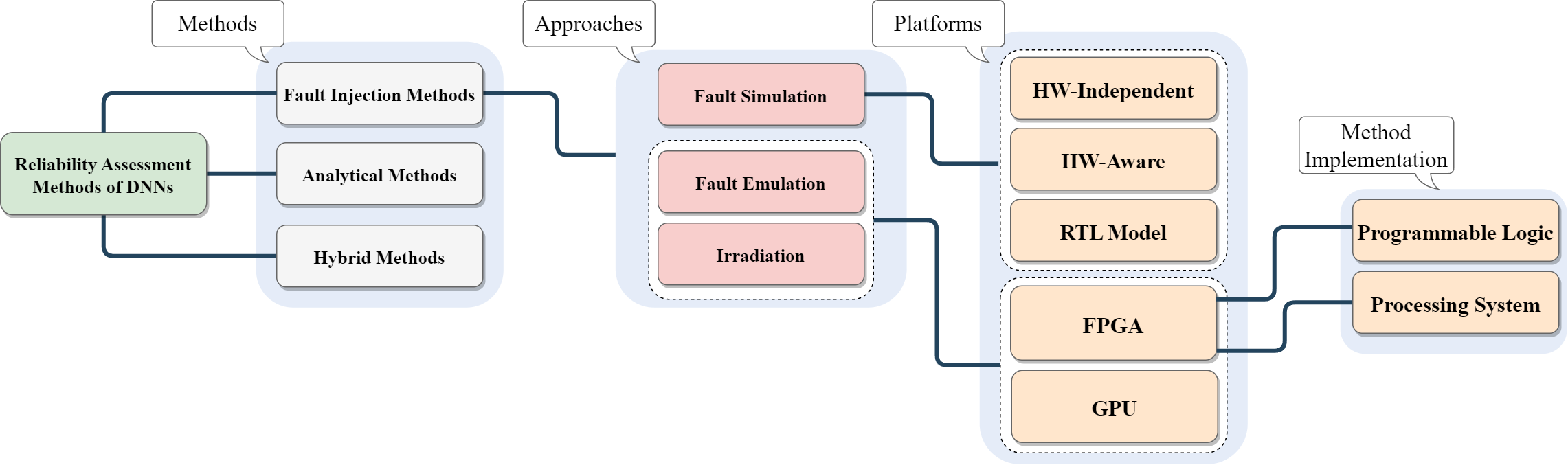
Figure 1: A taxonomy of DNN reliability assessment methods

A major consequence of single or multiple accumulated soft-error-caused bitflips affecting the weights of a given layer is their propagation as errors at the layer outputs (also known as layer Output Feature Map) and further throughout the subsequent layers, leading to incorrect DNN predictions. Fault resilience is the ability to tolerate the impact of faults on the output accuracy, and, in practice, it is one of the contributors to the final DNN accelerators’ reliability. A relevant mitigation strategy at the architecture level can be a hardening of the DNN, e.g., by layer redesign or selective hardening of neurons, such as hardened Processing Elements (PEs) or Triple Modular Redundancy (TMR) variants [8]. These imply the assessment of layers’ fault resiliency or identification of critical neurons in a neural network that are the most vulnerable to faults [27, 28, 29]. Fig. 1 presents a taxonomy for DNN reliability assessment methods. Along with analytical and hybrid methods [29], Fault Injection (FI) is a commonly used method for evaluating the fault resilience of DNNs [11, 30, 31]. The industry often employs fault injection by emulation in hardware, particularly in FPGAs, as it allows for evaluating real-scale DNN accelerator designs in significantly shorter run times than software-based simulations [9].

Fiji-FIN [32] is a representative framework implemented on the embedded Processing System for evaluating the resiliency of DNNs by emulating FI on FPGA. It measures accuracy degradation as a metric to study the impact of soft errors on network parameters. Designing fault injection campaigns for such frameworks requires significant effort, as each injection halts inference execution to manipulate DNN parameters. This interrupts classification time for a batch of inputs.

The state-of-the-art approaches for FI by emulation in FPGA using the embedded Processing System often require iterative procedures for each injected fault. In particular, such an iterative approach breaks the pipeline execution of the accelerator, requires a complex FI controller, and needs an extra FI control interconnection to handle the injection [33, 34, 32]. These procedures also involve multiple additional memory accesses, resulting in time-consuming processes and complex implementation.

Unlike the works mentioned above, our proposed method can be classified as fault injection by emulation in Programmable Logic. It leverages the functional approximation as a substitute for the errors generated by FI to improve processing and design time as well as the control complexity in the DNN fault resiliency analysis process. This approach allows the inference pipeline to be executed on a batch of inputs without interruption. This agile method enables a fast and efficient exploration of different options for network architecture, training, dataset selection, and more, to study the fault resilience of DNNs. Specifically, the introduced errors mimic single or multiple accumulated faults in weights. The method allows for efficient analysis of how subsequent layers in the network tolerate errors in the Output Feature Map of an assumed compromised layer are affected by faults in the weights of a compromised layer.

To the best of our knowledge, this is the first time that AxC units are utilized to enhance the efficiency and reduce the complexity of resilience analysis for DNNs.

III-B Proposed method

AxC is commonly used to approximate hardware components to improve compute efficiency while maintaining functional accuracy. However, in practice, the errors induced by approximation can be used to mimic the errors caused by faults in logic circuits. These errors affect the outputs of the corresponding units and propagate to subsequent layers, impacting their activations (Fig. 2). The proposed approach for evaluating DNN’s fault resiliency using approximate computing (AxC) units is presented in Fig. 2. To implement our proposed method, an AxMult, or an AxMult + a bit suppression unit (AxMult+) is implemented along with the exact implementation of the multipliers (ExMult) in the network, depending on whether the network is being run in functional or fault resilience assessment mode. The golden inference for the validation dataset is run only once, and the layer outputs are stored and compared with a Comparator unit. The Bit Suppressor unit is meant to increase the probability of more significant bits of the neuron being impacted by faults. The less significant bits of the layer Output Feature Map are already affected by the AxMult with proper randomness depending on the data distribution in the network and layers.

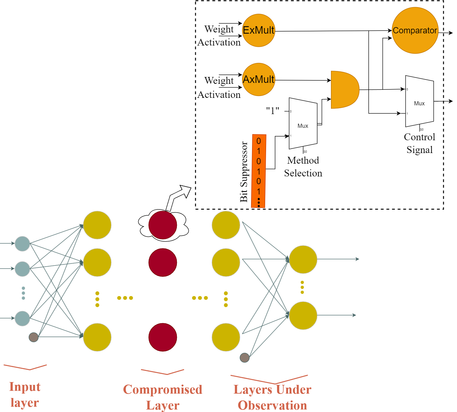
Figure 2: Proposed method evaluation

The overall flow of the proposed method is illustrated in Fig. 3. In Step 1, the user initializes the method by selecting the compromised layer in the DNN structure, the validation dataset (i.e., DNN inputs), and the application-specific target fault rate assumed for the analysis. In Step 2, suitable AxC units are selected for Approximate Processing Elements (AxPEs), such as the AxC multipliers from a relevant library, e.g., the EvoApproxLib [35], or their variants with bit suppression. In Step 3, the selected AxMults started executing the compromised layer by enabling corresponding AxPEs along with the Exact Processing Elements (ExPE) in the DNN architecture. The DNN inference is run while keeping the network pipeline intact, and the resulting DNN output accuracy drop is recorded as the primary metric for analyzing DNN fault resilience. A more significant drop in accuracy with induced errors implies a less fault-resilient DNN implementation. At the same time, the outputs of the AxMults are compared with the ExMults outputs to calculate the actual error at each neuron. The rest of the inference is executed by ExMults for both erroneous and exact outputs, and the comparison is performed for all the subsequent neurons of the network.

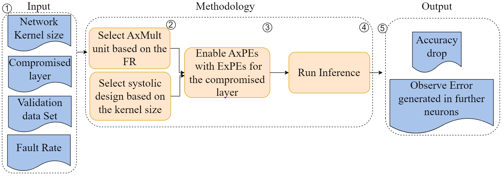
Figure 3: Methodology flow

The characteristics of the approximation-induced errors can be evaluated using different metrics such as normalized error, number of flipped bits, and impact on the neural network classification accuracy drop. In this study, we rely on a simple set of metrics that includes:

• Normalized error: the average error on the output of each layer is calculated by subtracting the neurons’ outputs of that layer from the golden output and dividing all the error values by the maximum value.

• Network accuracy: calculated by executing the network under different circumstances (faulty, AxMult, AxMult + bit suppressor and bit suppressor) over the test set.

• Bitflips in subsequent layers: calculated by comparing all bits in the next layers’ outputs with the golden model and counting the bits that do not match as flipped bits.

III-B1 Accelerator Model

Fig. 4 illustrates the accelerator model to perform resilience analysis on FPGA. It consists of two different systolic architecture designs based on the network under test. The $N\times N$ systolic architecture is used based on the convolution layers’ kernel size to perform the most optimum dot matrix. At the same time, all designs have ExPE and AxPE to perform the resilience analysis and benefits of a dual register to store the results of both approximate systolic and exact systolic for further comparisons. An Error Detector (ED) module is also provided to compute the error generated at each neuron’s output compared to the exact output and can be used for the neuron’s vulnerability evaluation.

This implementation provides us following features:

1. Understanding the vulnerability of neurons by computing the error generated through the hardware and further layers by comparing the exact and approximate systolic design outputs;

2. Increasing the controllability for enabling errors in each layer individually and keeping the other layers correct;

3. Eliminating the need for designing and deploying an extra complex controller for the fault injection procedure. A simple approximate unit enabling circuitry is employed instead;

4. The inference pipeline process executes a batch of inputs with no need to break this process;

5. The resilience assessment process is performed without an extra interconnect for weight sampling;

6. The proposed approach is not iterative for each potential fault location (unlike the traditional fault injection). Thus, the analysis complexity is vastly reduced.

Note that the features (c)-(f) are specific for FI emulation in Programmable Logic and generally not available in Processing Logic based methods such as Fiji-FIN.

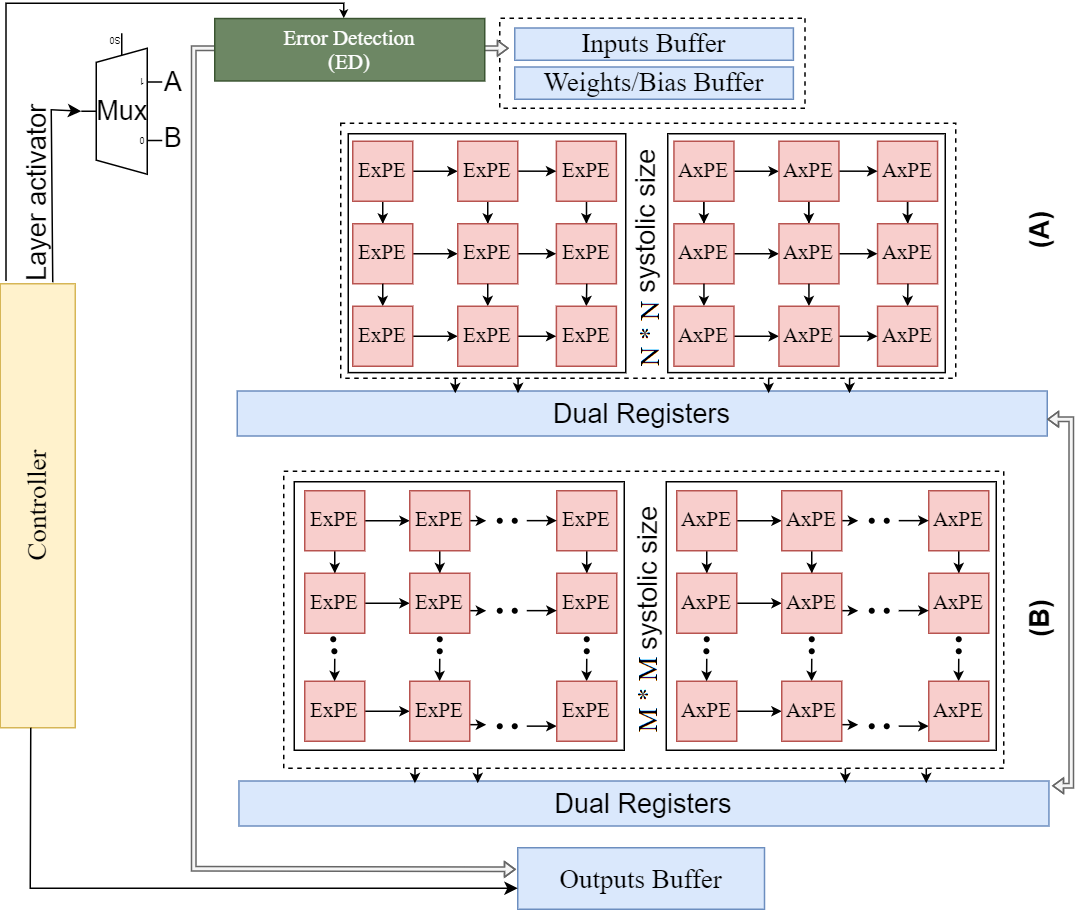
Figure 4: Proposed systolic architecture for our Resiliency assessment DNN accelerator framework

III-C Experimental Results

III-C1 Evaluation methodology

To assess the feasibility of the proposed method, we implemented the same flow as shown in Fig. 2 with fault injection (FI). Using Table I, we narrowed down the list of candidate approximate multipliers from the EvoApproxLib library [35] based on several relevant metrics, with a primary focus on two established features, namely, the Variance of Error Distance (Var-ED) and Root Mean Square (RMS-ED) presented in [36]. These metrics are crucial in determining the approximation-induced errors that affect the performance of an AxC unit in DNNs. We selected mul8s_1L2N for the experiment based on these metrics and results achieved from the high-level experiments on the network through the proposed GPU accelerated framework for CNN approximation in Section II.

For the reference part, we repeated the fault resiliency evaluation on the original network, which was instrumented with a state-of-the-art FI method [32]. In this study, we considered the injection of multiple bitflips at a random location in all OFM’ bits of the compromised layer for every input in the DNN validation test set. In this case, we assumed that 10% of the weights’ bits were faulty.

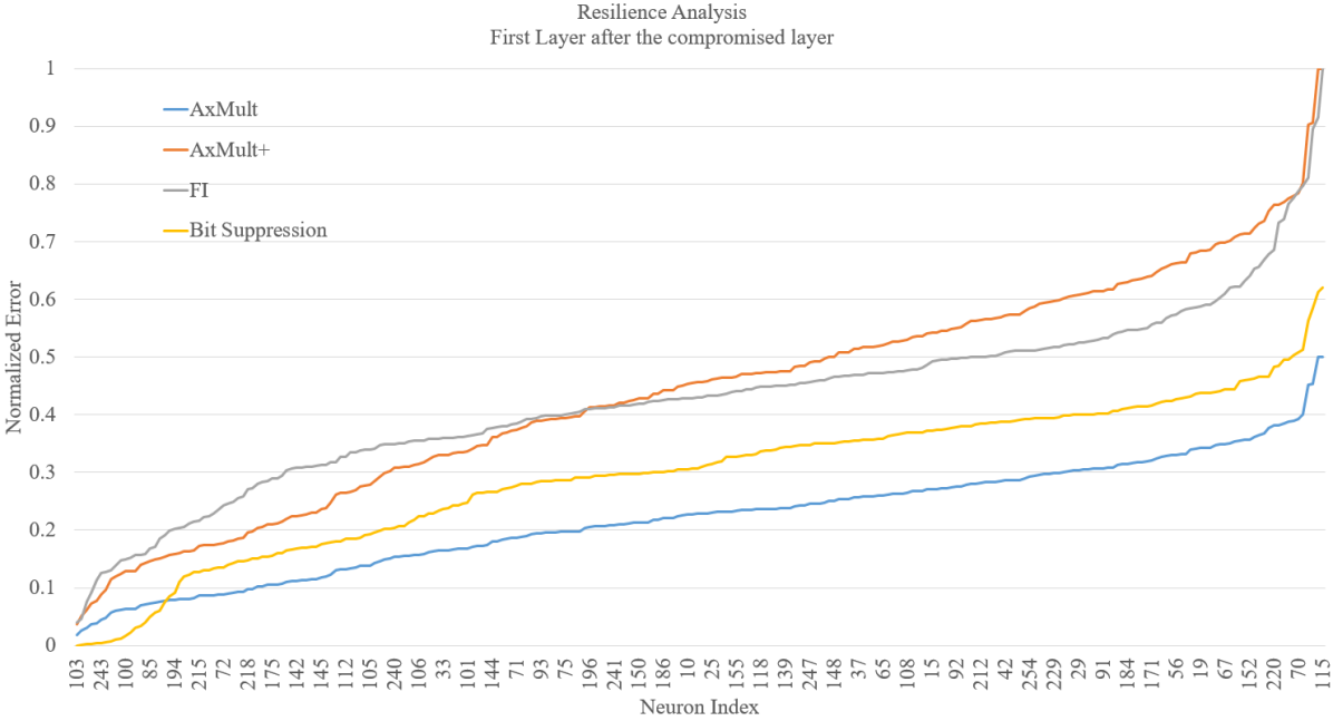
Figure 5: Normalized output error of Pool2: Applying AxMult, AxMult+ , Bit Suppression and FI on the Conv1

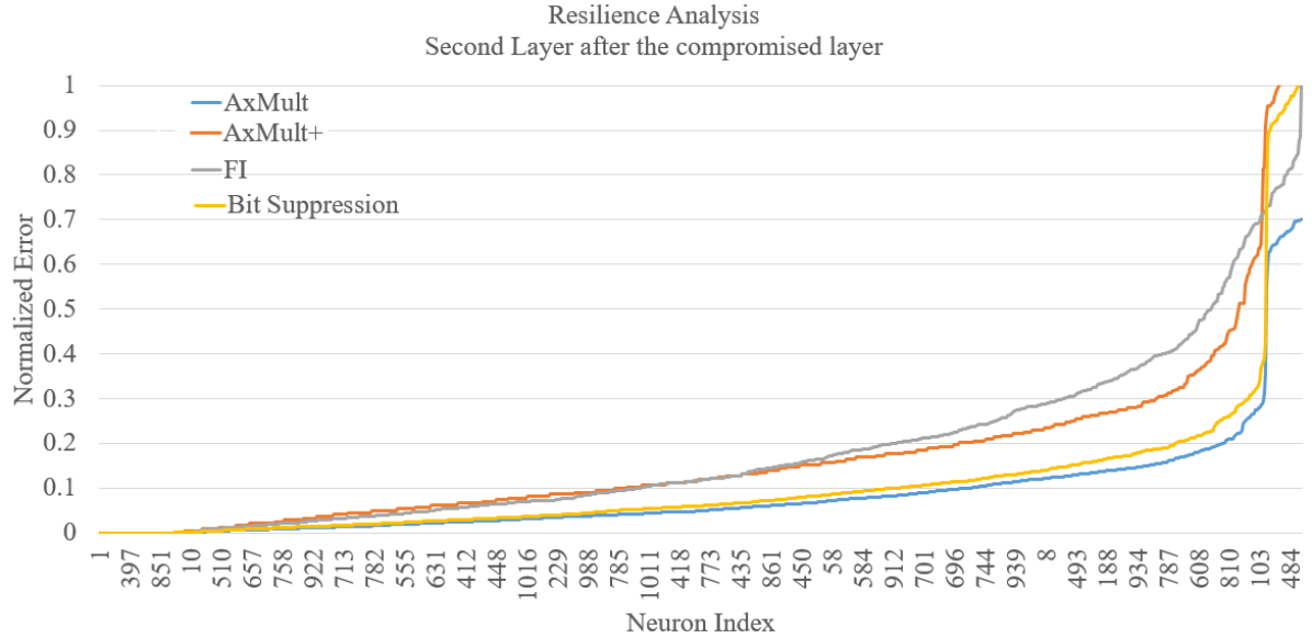
Figure 6: Normalized output error of Conv2: Applying AxMult, AxMult+ , Bit Suppression and FI on the Conv1

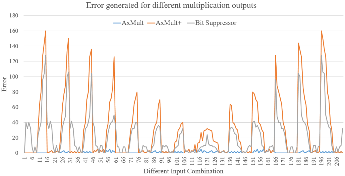
Figure 7: Multiplication output error generated by AxMult, AxMult+ and Bit Suppression

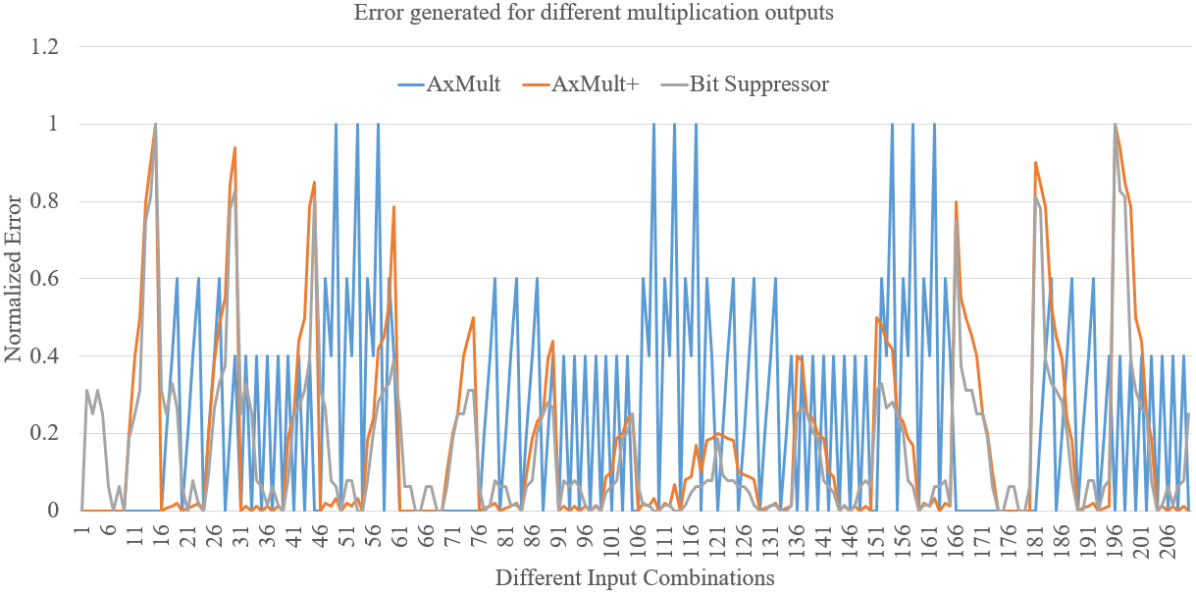
Figure 8: Normalized Multiplication output error generated by AxMult, AxMult+, and Bit Suppression

To achieve a high FI confidence level using the statistical fault injection approach [37], we repeated the experiment for each fault model with 1000 random faults per image. The average accuracy of all repetitions was then reported.

We evaluated the impact of AxMult, AxMult + Bit Suppression (AXMult+), Bit Suppression alone, and fault injection, along with normalized error and the number of flipped bits, on the DNN accuracy. The results show a drop in DNN accuracy due to these factors. We compared the normalized error and the number of flipped bits for each scenario.

III-C2 Experimental Setup

To evaluate the feasibility of the proposed method, a case-study Convolutional Neural Network (CNN) with two convolutional layers, two max-pooling, and one Fully-Connected (FC) layer was implemented and trained. The simulations were performed on an Intel® Core™ i7-6800K CPU @ 3.40GHz × 12, and the proposed method was implemented with Python 3. The hardware synthesis and implementation results are produced by the Xilinx Vivado HLS tool on a Xilinx Versal VCK190 FPGA (xcvc1902-vsva2197-2MP-e-S) at 166 MHz operational frequency.

The CNN under study is trained on a dataset of 2000 images of animals (cats and dogs) and humans for binary classification. The accuracy of the network over the test set (including 450 images of animals and humans) is 93.34%. Bit truncation quantization is applied in network parameters during training, and data precision is reduced to 8-bit.

III-C3 Evaluation Results

We analyzed the similarity of the fault resiliency analysis results obtained by fault emulation and our proposed method using the metrics identified in Section III-B.

Fig. 6 shows the distribution of normalized error in the output of the second convolutional layer (Conv2) in the presence of 10% random faults in the first convolution layer (grey), errors induced by AxMult (blue), and errors induced by AxMult + bit suppressor (orange) enabled in the first convolution layer, respectively. Fig. 6 reports the impact of applying FI and our proposed method on the same convolutional layer and its effect on the second pooling layer of the network. These results demonstrate the similarity in error propagation trends between the proposed and reference methods.

In practice, by analyzing these charts, users can set a criticality threshold on the output error of the neurons based on their application and determine the number and indices of neurons to be used for any protection techniques. Generally, if we set the threshold at some error value, all methods suggest some neuron indices for mitigation techniques. As it can be concluded, both AxMult + bit suppression and FI show very similar behaviors. However, relying solely on the AxMult or bit suppression techniques is quite inaccurate for high fault ratios like this case study here.

For example, by setting the error threshold to 0.7, FI will recommend the user to protect 50 out of 1024 neurons of the Conv2 network’s second CONV’s neurons, while AxMult + bit suppression will recommend 53 out of 1024 neurons, including all the critical neurons recognized by FI. Fig. 8 and Fig. 8 show the error distribution of the three different methods, i.e., AxMult, AxMult + bit suppressor, and bit suppressor on the output of a multiplication operation with all the combinations of two 8-bit inputs. From Fig. 8, it is evident that the error values generated by AxMult + bit suppressor can almost cover a vast range of different values, and Fig. 8 shows that the error is evenly distributed on all different input combinations.

Table. III is reporting the number of bitflips and accuracy drop in subsequent layers caused by the compromised first convolution layer. These results also demonstrate the strong similarity of the trends in error propagation by the AxMult and its variants with the reference method. In case of accuracy drop, AxMult + bit suppression shows a strong correlation with the FI method and surpasses the other two methods.

Table IV reports details of the hardware accelerator implementation. Based on the results, the proposed implementation can be executed on the FPGA at 166 MHz clock frequency, and only by using $\sim$16% of the available LUTs on the board all three mentioned systolic-array size architectures can be implemented to improve the efficiency of the accelerator. The timing comparison of the proposed method and the state-of-the-art fault injection method are presented in Table. V. As it can be concluded, by keeping an acceptable accuracy of FI in identifying the critical neurons, we get thousands of times speed-up in the resilience assessment of the DNNs. (Specifically, it is 5417 times in this example). At the same time, the proposed method does not need extra interconnects to manage the assessment process, and the original controller of the accelerator can take care of the fault resiliency assessment process.

TABLE III: Bitflips and Accuracy drop induced by our proposed method vs. the reference fault injection method by fault rate 10% in OFM of the first convolution layer

Measured Layer	Bitflips in subsequent layers
	FI (reference) [%]	AxMult [%]	AxMult+ [%]	Bit suppressor [%]
Conv1	10	10.30	10	10.20
Pool1	9.07	9.20	9.06	9.15
Conv2	16.76	16.80	16.77	16.83
Pool2	16.51	16.66	16.53	16.62
Accuracy drop [%]
	16.73	9.33	18.33	24.73

TABLE IV: Hardware implementation of the proposed hardware accelerator

	Resource Utilization (%)
Conv2D systolic size	LUT	FF	BRAM	Data Path Delay	CLK Frequency
3*3	0.03	0.00	0.83	Logic: $\sim$20% Route: $\sim$80%	166 MHz
5*5	0.09	0.00	0.83
32*32	15.30	0.91	0.85

TABLE V: Timing overheads of the proposed method vs. the reference fault injection method (Conv1 layer)

Network	Analysis Control Circuitry	Interconnects	DNN execution time in FPGA
Base CNN	N/A	Data Exchange Interconnect	$\sim$120ms
Fault Resilience Assessment
CNN instrumented with FI	Complex FI Controller	(Data Exchange + FI) Interconnect	$\sim$650,000ms
CNN instrumented with AxMult+	Accelerator Controller	Data Exchange Interconnect	$\sim$120ms

IV Fault resiliency in DNNs

IV-A Motivations and Related Works

In the last few years, researchers have investigated the theory behind brain-inspired computational models to build artificial structures capable of addressing highly complex computational problems. Today, DNNs are considered attractive solutions in several fields due to their outstanding computational capabilities as well as their human-level performance. The human brain is a complex and fascinating system able to bear synapses or neuron faults and still keep working properly, thanks to its plastic ability to remodel, repair, and reorganize its neural functions. Similarly, artificial neural networks possess in their structure a certain degree of redundancy that leads to intrinsic robustness and resilience against the occurrence of faults. This is caused by two aspects: the first is related to their distributed and parallel structure; the second to the redundancy resulting from the over-provisioning [38]. Indeed, neural networks are furnished with a quantity of artificial neurons higher than the minimal number required to perform a computation. It means that they can bear a bounded number of errors thanks to the excessive neuron budget: once this number is exceeded, the precision degrades gracefully as the number of errors increases [39].

This structural feature allows them to have an attractive property known as masking ability, which corresponds to the ability of DNNs to stop the propagation of some faults by masking their effects. As an example, it has been shown that the presence in DNNs of the Rectified Linear Unit (ReLU) activation function halves the percentage of critical faults by stopping the propagation of faults on negative weights [40]. Understanding how faults propagate through the neural network is very important, as it may influence: the reliability assessment procedure; efficient fault detection and mitigation strategies.

The analysis of fault propagation in DNNs has been conducted in the literature by different perspectives. A preliminary theory-driven analysis is proposed in [41], where the authors explore inherent characteristics of fault propagations in DNNs from the theoretical aspect. They propose a formula to compute the perturbation caused by the i-th bit flip on a weight represented in a 32-bit floating-point format. The authors in [42] characterize the propagation of soft errors from the hardware to the application software of DNN systems. Based on this, they devise cost-effective solutions to mitigate Silent Data Corruption (SDC) in software and hardware. Further studies on faults propagations in DNNs are described in [43] and [44].

Nevertheless, it is important to underline that the major effort in the above-mentioned research works consists in understanding how critical faults (i.e., those that lead to application failures) propagate through the hardware-software system.

The intent of this section is twofold. On the one hand, it aims to show how a critical fault spreads through a network. On the other hand, this section tackles the problem from a different angle, showing how a masked fault is propagated within the system, analysing the role DNNs have in this process. The investigation of this latter category of faults is important for the following reasons:

• In a fault injection process, the identification of sets of faults that are masked may reduce the fault space and, as a consequence, lower the costs of the reliability assessment;

• In the design of DNN models, the knowledge of architectural elements that favour the masking ability of DNNs can lead to the design of more robust models.

This section presents an analysis on masked faults with the goal of identifying at what point in the computation their propagation is stopped and if it is possible to know in advance their effects on the output of the DNN.

IV-B Proposed Method

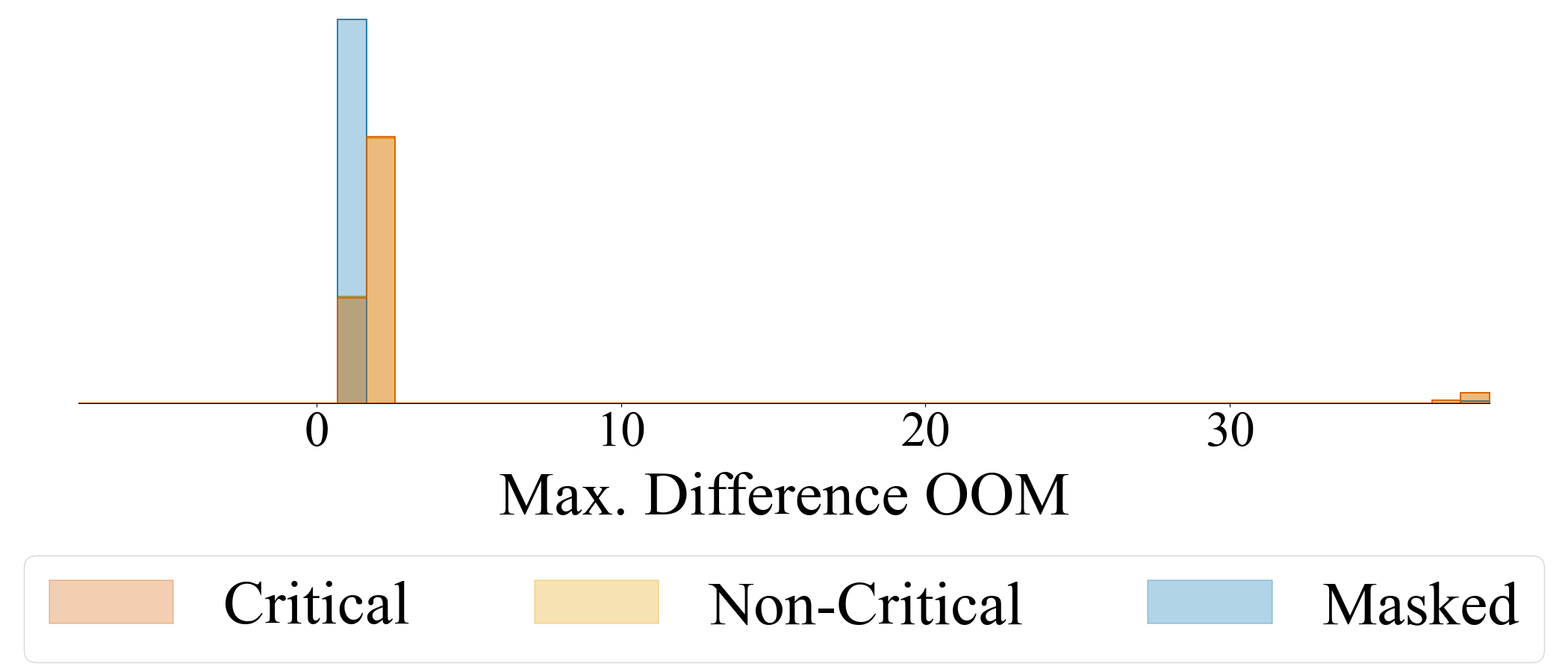
(a) LeNet5: Max. Difference

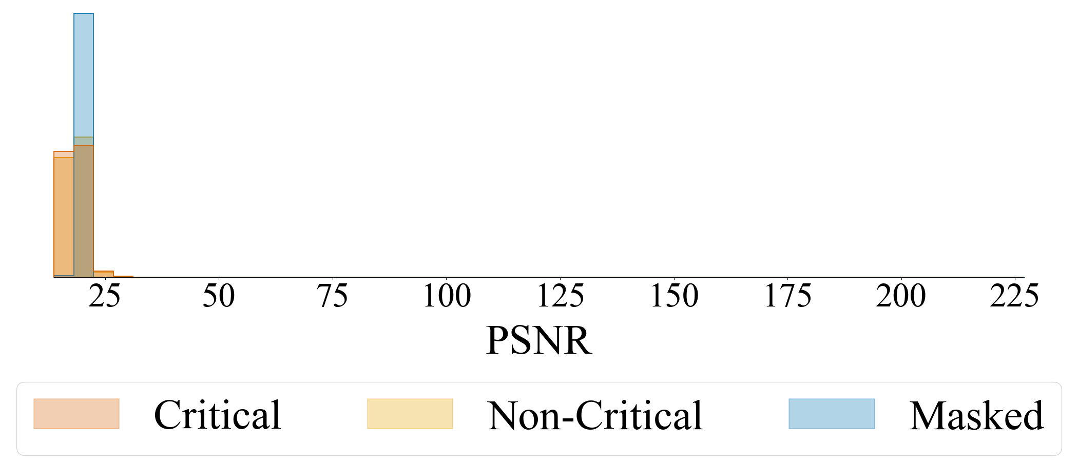
(b) LeNet5: PSNR

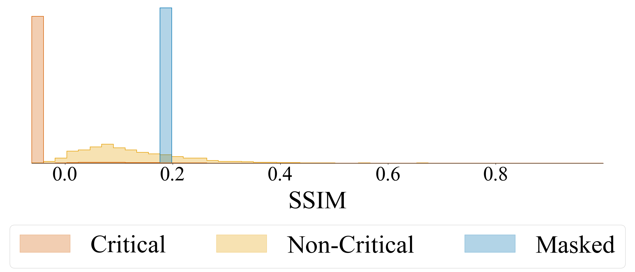
(c) LeNet5: SSIM

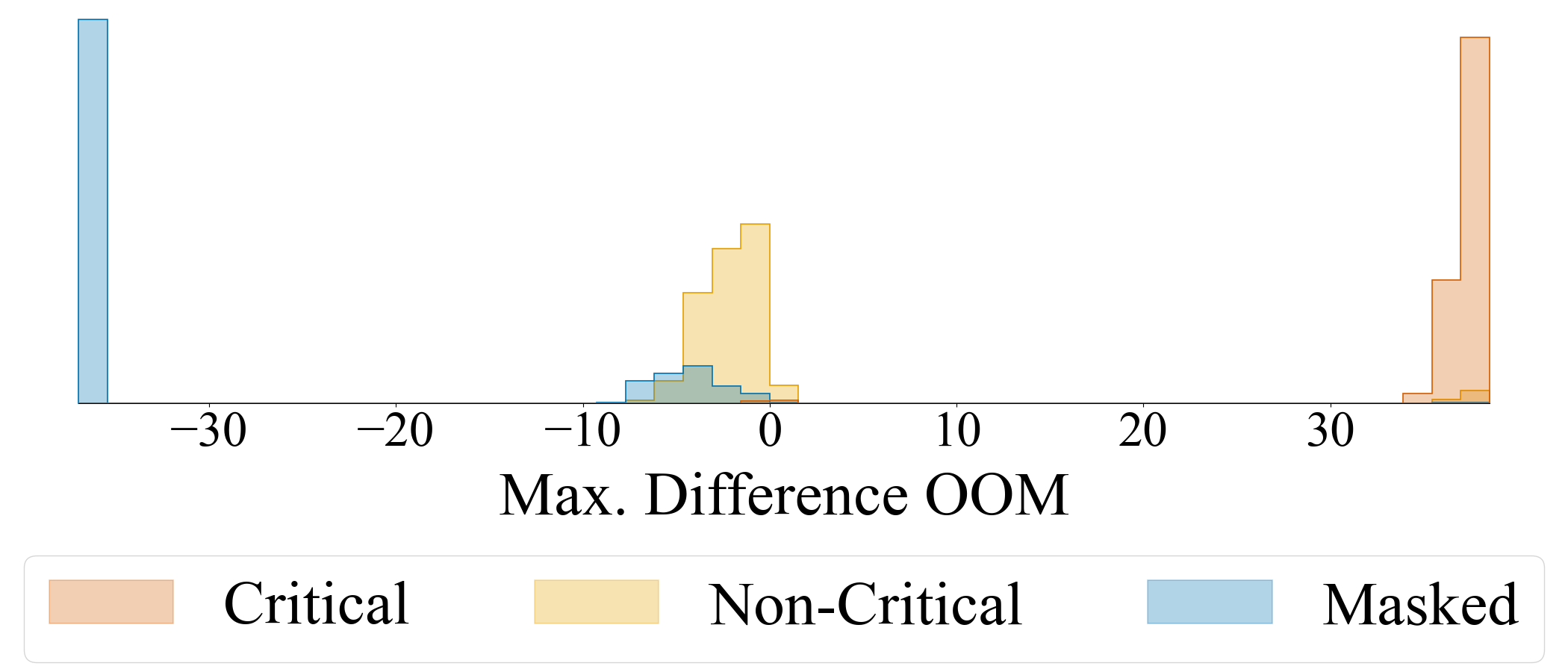
(d) ResNet20: Max. Difference

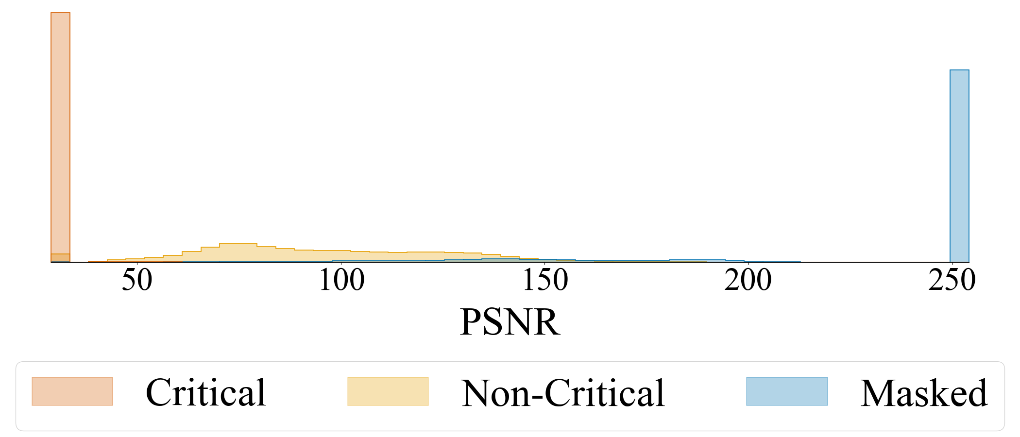
(e) ResNet20: PSNR

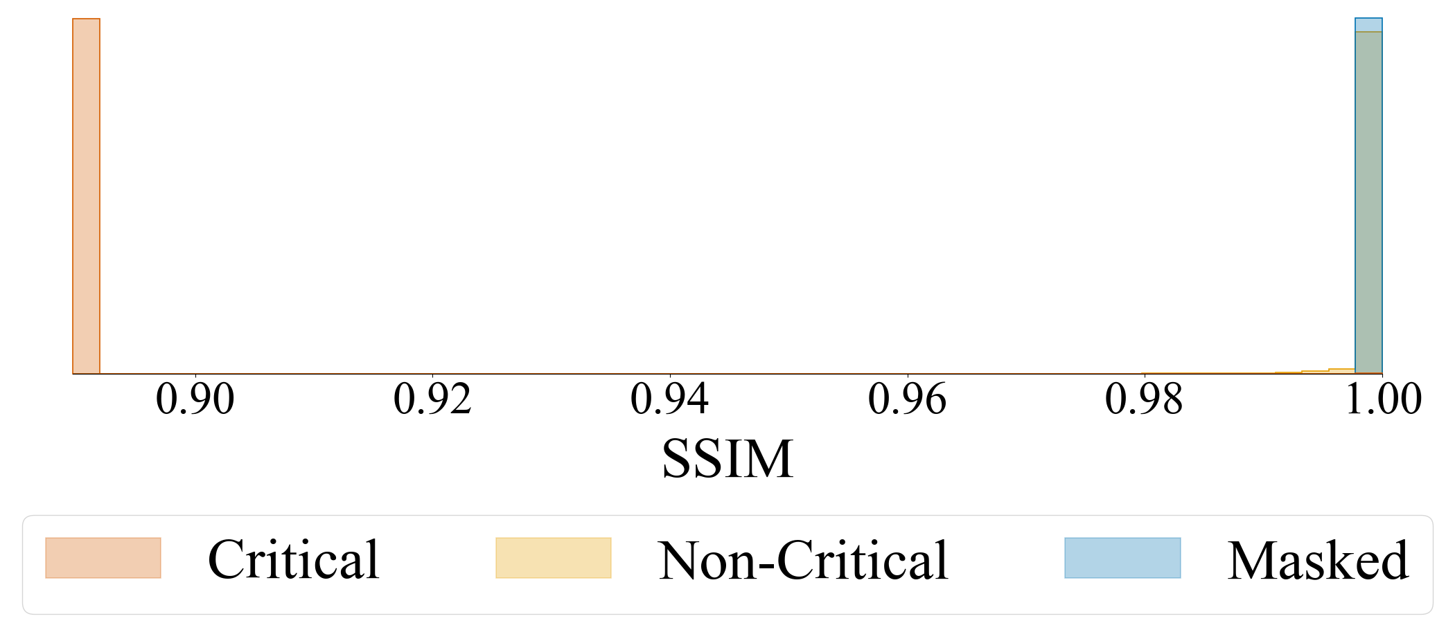
(f) ResNet20: SSIM

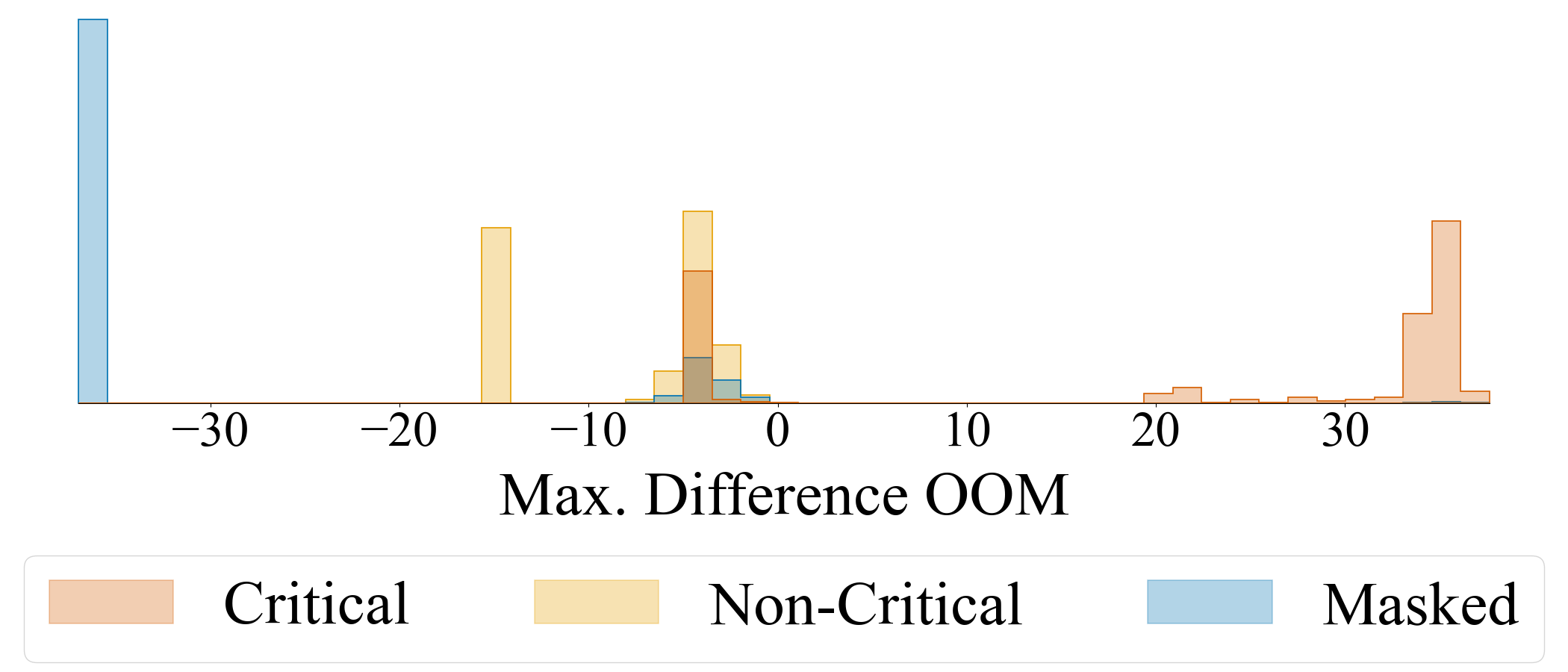
(g) DenseNet121: Max. Difference

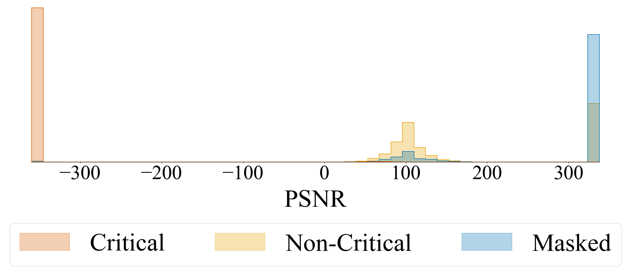
(h) DenseNet121: PSNR

(i) DenseNet121: SSIM

Figure 9: Metric probability distributions for the CNN under exam, observed in the layer where the fault is injected. Figures (a)-(c) refer to LeNet-5, Figures (d)-(f) refer to ResNet20 and Figures (g)-(i) refer to DenseNet121.

CNNs are a subset of DNNs composed of a set of convolutional layers. The output of each layer is a multidimensional tensor, often referred to as the Output Feature Map (OFM). In the field of Image Classification, the output of the network is represented by a vector called logit. A fault affecting a CNN can be classified as:

• Critical, if it causes a change in the network prediction;

• Non-Critical, if it impacts the logit without changing the prediction;

• Masked, if it does not modify the logit.

When a fault affects the parameters of a layer (i.e., weights), it may change its OFM, as well as the one of all the following layers. If the fault is masked, the difference between the golden Output Feature Map (gOFM) and the faulty Output Feature Map (fOFM) of the impacted layer should be small or zero. Contrarily, it is logical to assume that a critical fault also produces a fOFM that is radically different from the gOFM.

As a consequence of these two observations, it is possible to predict the impact of a fault without needing to carry out a complete inference. In fact, this section aims at showing that:

1. Masked faults, once triggered, rarely propagate for more than one layer. Thus, the only different OFM is the one of the layer directly affected by the fault;

2. Critical faults, can be immediately identified by performing some early measures, using some metrics that can be computed by comparing the fOFM and the gOFM of the affected layer.

The OFM of a layer $l$ can be interpreted as a collection of $n$ filtered images, where $n$ is the number of filters applied in layer $l$. Furthermore, the fOFM resulting from a fault in the network parameters can be interpreted as the gOFM plus a Gaussian noise. Therefore, it is possible to apply well-known objective image quality metrics, such as the Peak signal-to-noise Ratio (PSNR) and the Structural Similarity Index Metric (SSIM) [45].

This section proposes to use three different metrics to predict the criticality of a fault, starting from the OFM of the affected layer.

IV-B1 Max Difference

This first metric computes the maximum distance between the gOFM and the fOFM. This metric is presented as a baseline since, to the best of the authors’ knowledge, there are no metrics that correlate the criticality of a fault with the changes in the OFM.

IV-B2 PSNR

This metric is directly proportional to the ratio between the peak signal (i.e., the maximum element of the gOFM) and the power of the corrupting noise, represented by the mean square error between the gOFM and the fOFM. The value can be computed as follows:

$$PSNR=10\cdot\log_{10}\frac{\max(gOFM)^{2}}{MSE(gOFM,fOFM)}$$ (1)

Where $\max(gOFM)$ is the maximum value of the gOFM and $MSE$ is the Mean Square Error between the gOFM and the fOFM.

IV-B3 SSIM

this metric improves the PSRN, by including the concept of structural information, represented by the relationship of a neuron with its neighbours. The formula is composed by the product of three terms, the luminance, the contrast and the structural term. In the context of the study of the OFM, the simplified formula can be expressed as:

$$SSIM=\frac{(2\mu_{f}\mu_{g}+C_{1})(2\sigma_{fg}+C_{2})}{(\mu_{f}^{2}+\mu_{g}^{2}+C_{1})(\sigma_{f}^{2}+\sigma_{g}^{2}+C_{2})}$$ (2)

Where $\mu_{g},\mu_{f}$ are the mean of the gOFM and of the fOFM, $\sigma_{g},\sigma_{f}$ their standard deviation, $\sigma_{fg}$ their cross-covariance. $C_{1}$ and $C_{2}$ are two regularization parameters.

IV-C Experimental Results

This section analyses three different CNNs used for Image Classification to study how a fault can propagate. The networks under analysis are: LeNet-5 with the MNIST dataset, ResNet20 with CIFAR-10 and Densenet-121 with ImageNet. For each network, we performed a statistical FI as described in [46]. The tool used to carry out the FI campaign is SCI-FI [47], that allows to speed up the FI process using the Fault Dropping and the Delayed Start techniques. The faults injected are single bit-flips in the network parameters, represented as 32-bit floating points. Further details on the networks under exam and on the FI campaigns are reported in Table VI.

TABLE VI: The networks under analysis

Network	Dataset	Dataset Size	Acc. [%]	Weights	Injected Faults
LeNet5	MNIST	10,000	98.85	61,706	2,212
ResNet20	CIFAR-10	10,000	91.72	269,722	15,675
DenseNet121	ImageNet	50,000	74.43	7,978,856	16,685

Firstly, to demonstrate that Masked faults only modify the OFM of the layer affected by the fault, we report the percentage of Masked faults that affect more than one layer. In particular, for LeNet5, all the Masked faults do not modify any OFM besides the one of the impacted layer. For ResNet20, $87.99\%$ of Masked faults show no effect in the OFM of the layer immediately after the impacted one, while for DenseNet this number rises to $99.17\%$.

To show that Critical faults have a strong impact early on, we compute the metrics introduced in Section IV-B on the OFM of the layer affected by the fault. Figure 9 reports the metrics distributions for the Max Difference, the PSNR and the SSIM. Each image shows, for each network, the distribution of a metric computed for all the FI campaigns. In particular, the distribution is further subdivided according to the impact of the fault affecting the network when they were measured. This means that the distribution labelled ’Critical’ reports only the value measured when a Critical fault is affecting the network. For a metric, the more separable the three distributions are, the better the metric is at predicting the effect of a fault.

In particular, we can observe a stark contrast between the metrics computed for LeNet5 and the other networks. This can be imputed to the lack of batch-normalization layers, that normalize the value of the weights (and of the OFM) between $[-1,1]$. Consequently, even a bit-flip in the mantissa bits of the weight can have a large impact. Nonetheless, SSIM performs sufficiently well, as it correctly separates Critical and Non-Critical faults.

For the other two CNNs, we can notice that both the Max. Difference and the PSNR separate Masked faults from Critical and Non-Critical faults. However, for ResNet20, SSIM outperforms the other metrics, as it completely splits ups Critical and Non-Critical faults while providing a good degree of separation between Masked and Non-Critical faults. Contrarily, for DenseNet-121, SSIM does not completely separate Masked from Critical. For this latter network, the best solution is offered by the PSNR.

Therefore, we observe how different metrics can correctly predict Masked and Critical faults without the need for a complete inference, by simply analysing the fOFM of the layer affected by the fault.

As a final note, we want to highlight that the cost of the computation of the metric is quite small, requiring only a portion of the time required for the computation of a whole layer. On average, the per-layer overhead added by the computation of one of the metrics is $76.51\%$ for LeNet5 $74.28\%$ for ResNet20 and $73.54\%$ for DenseNet121.

V Conclusions

This paper explored approximation and fault resiliency of DNN accelerators. To allow fast evaluation of AxC DNN, an efficient GPU-based simulation framework was developed. The paper proposed a method for employing approximate (AxC) arithmetic circuits to agilely emulate errors in hardware without performing fault injection on the DNN. Finally, it presented a fine-grain analysis of fault resiliency by examining fault propagation and masking in networks.

References

- [1] V. Sze, Y.-H. Chen, T.-J. Yang, and J. S. Emer, “Efficient processing of deep neural networks: A tutorial and survey,” Proceedings of the IEEE, vol. 105, no. 12, pp. 2295–2329, 2017.
- [2] G. Armeniakos, G. Zervakis, D. Soudris, and J. Henkel, “Hardware approximate techniques for deep neural network accelerators: A survey,” ACM Computing Surveys, vol. 55, no. 4, pp. 1–36, 2022.
- [3] A. Bosio, D. Ménard, and O. Sentieys, Eds., Approximate Computing Techniques. Springer International Publishing, 2022. [Online]. Available: https://doi.org/10.1007/978-3-030-94705-7
- [4] A. Nardi and A. Armato, “Functional safety methodologies for automotive applications,” in 2017 IEEE/ACM International Conference on Computer-Aided Design (ICCAD). IEEE, 2017, pp. 970–975.
- [5] M. Jenihhin, M. S. Reorda, A. Balakrishnan, and D. Alexandrescu, “Challenges of reliability assessment and enhancement in autonomous systems,” in 2019 IEEE International Symposium on Defect and Fault Tolerance in VLSI and Nanotechnology Systems (DFT), 2019, pp. 1–6.
- [6] M. Shafique, M. Naseer, T. Theocharides, C. Kyrkou, O. Mutlu, L. Orosa, and J. Choi, “Robust machine learning systems: Challenges, current trends, perspectives, and the road ahead,” IEEE Design & Test, vol. 37, no. 2, pp. 30–57, 2020.
- [7] A. Bosio, P. Bernardi, A. Ruospo, and E. Sanchez, “A reliability analysis of a deep neural network,” in 2019 IEEE Latin American Test Symposium (LATS). IEEE, 2019, pp. 1–6.
- [8] S. Mittal, “A survey on modeling and improving reliability of dnn algorithms and accelerators,” Journal of Systems Architecture, vol. 104, p. 101689, 2020.
- [9] Y. Ibrahim, H. Wang, J. Liu, J. Wei, L. Chen, P. Rech, K. Adam, and G. Guo, “Soft errors in dnn accelerators: A comprehensive review,” Microelectronics Reliability, vol. 115, p. 113969, 2020.
- [10] C. Torres-Huitzil and B. Girau, “Fault and error tolerance in neural networks: A review,” IEEE Access, vol. 5, pp. 17 322–17 341, 2017.
- [11] F. Su, C. Liu, and H.-G. Stratigopoulos, “Testability and dependability of ai hardware: Survey, trends, challenges, and perspectives,” IEEE Design & Test, 2023.
- [12] L. M. Luza, D. Söderström, G. Tsiligiannis, H. Puchner, C. Cazzaniga, E. Sanchez, A. Bosio, and L. Dilillo, “Investigating the impact of radiation-induced soft errors on the reliability of approximate computing systems,” in 2020 IEEE International Symposium on Defect and Fault Tolerance in VLSI and Nanotechnology Systems (DFT). IEEE, 2020, pp. 1–6.
- [13] M. Taheri, M. Riazati, M. H. Ahmadilivani, M. Jenihhin, M. Daneshtalab, J. Raik, M. Sjõdin, and B. Lisper, “Deepaxe: A framework for exploration of approximation and reliability trade-offs in dnn accelerators,” in 24th International Symposium on Quality Electronic Design. https://doi.org/10.48550/arXiv.2303.08226, 2023.
- [14] M. Pinos, V. Mrazek, F. Vaverka, Z. Vasicek, and L. Sekanina, “Acceleration techniques for automated design of approximate convolutional neural networks,” IEEE Journal on Emerging and Selected Topics in Circuits and Systems, pp. 1–1, 2023.
- [15] A. Ruospo, L. M. Luza, A. Bosio, M. Traiola, L. Dilillo, and E. Sanchez, “Pros and cons of fault injection approaches for the reliability assessment of deep neural networks,” in 2021 IEEE 22nd Latin American Test Symposium (LATS). IEEE, 2021, pp. 1–5.
- [16] A. Bosio, I. O’Connor, M. Traiola, J. Echavarria, J. Teich, M. A. Hanif, M. Shafique, S. Hamdioui, B. Deveautour, P. Girard et al., “Emerging computing devices: Challenges and opportunities for test and reliability,” in 2021 IEEE European Test Symposium (ETS). IEEE, 2021, pp. 1–10.
- [17] M. A. Talib, S. Majzoub, Q. Nasir, and D. Jamal, “A systematic literature review on hardware implementation of artificial intelligence algorithms,” The Journal of Supercomputing, vol. 77, pp. 1897–1938, 2021.
- [18] M. Barbareschi, S. Barone, and N. Mazzocca, “Advancing synthesis of decision tree-based multiple classifier systems: an approximate computing case study,” Knowledge and Information Systems, pp. 1–20, Apr. 2021, company: Springer Distributor: Springer Institution: Springer Label: Springer Publisher: Springer London. [Online]. Available: https://link.springer.com/article/10.1007/s10115-021-01565-5
- [19] M. Barbareschi, S. Barone, A. Bosio, J. Han, and M. Traiola, “A Genetic-algorithm-based Approach to the Design of DCT Hardware Accelerators,” ACM Journal on Emerging Technologies in Computing Systems, vol. 18, no. 3, pp. 1–25, Jul. 2022. [Online]. Available: https://dl.acm.org/doi/10.1145/3501772
- [20] M. Barbareschi, S. Barone, N. Mazzocca, and A. Moriconi, “A Catalog-based AIG-Rewriting Approach to the Design of Approximate Components,” IEEE Transactions on Emerging Topics in Computing, 2022.
- [21] A. Bosio, D. Ménard, and O. Sentieys, Eds., Approximate Computing Techniques: From Component- to Application-Level. Cham: Springer International Publishing, 2022. [Online]. Available: https://link.springer.com/10.1007/978-3-030-94705-7
- [22] V. Mrazek, Z. Vasicek, L. Sekanina, H. Jiang, and J. Han, “Scalable Construction of Approximate Multipliers With Formally Guaranteed Worst Case Error,” IEEE Transactions on Very Large Scale Integration (VLSI) Systems, vol. 26, no. 11, pp. 2572–2576, Nov. 2018, conference Name: IEEE Transactions on Very Large Scale Integration (VLSI) Systems.
- [23] Y. Lecun, L. Bottou, Y. Bengio, and P. Haffner, “Gradient-based learning applied to document recognition,” Proceedings of the IEEE, vol. 86, no. 11, pp. 2278–2324, Nov. 1998, conference Name: Proceedings of the IEEE.
- [24] K. He, X. Zhang, S. Ren, and J. Sun, “Deep Residual Learning for Image Recognition,” in 2016 IEEE Conference on Computer Vision and Pattern Recognition (CVPR). Las Vegas, NV, USA: IEEE, Jun. 2016, pp. 770–778. [Online]. Available: http://ieeexplore.ieee.org/document/7780459/
- [25] Y. LeCun, C. Cortes, and C. Burges, “MNIST Handwritten digit database,” 1998. [Online]. Available: http://yann.lecun.com/exdb/mnist/
- [26] A. Krizhevsky, V. Nair, and G. Hinton, “CIFAR-10 (canadian institute for advanced research),” 2010. [Online]. Available: https://www.cs.toronto.edu/ kriz/cifar.html
- [27] C. Schorn et al., “Accurate neuron resilience prediction for a flexible reliability management in neural network accelerators,” in 2018 DATE. IEEE, 2018, pp. 979–984.
- [28] A. Ruospo and E. Sanchez, “On the reliability assessment of artificial neural networks running on ai-oriented mpsocs,” Applied Sciences, vol. 11, no. 14, p. 6455, 2021.
- [29] M. H. Ahmadilivani, M. Taheri, J. Raik, M. Daneshtalab, and M. Jenihhin, “Deepvigor: Vulnerability value ranges and factors for dnns’ reliability assessment,” arXiv preprint arXiv:2303.06931, 2023.
- [30] A. Ruospo, E. Sanchez, L. M. Luza, L. Dilillo, M. Traiola, and A. Bosio, “A survey on deep learning resilience assessment methodologies,” Computer, vol. 56, no. 2, pp. 57–66, 2023.
- [31] M. Taheri, M. H. Ahmadilivani, M. Jenihhin, M. Daneshtalab, and J. Raik, “Appraiser: Dnn fault resilience analysis employing approximation errors,” in 26th International Symposium on Design and Diagnostics of Electronic Circuits and Systems. In press, 2023.
- [32] N. Khoshavi, C. Broyles, Y. Bi, and A. Roohi, “Fiji-fin: A fault injection framework on quantized neural network inference accelerator,” in 2020 19th IEEE International Conference on Machine Learning and Applications (ICMLA). IEEE, 2020, pp. 1139–1144.
- [33] M.-C. Hsueh, T. K. Tsai, and R. K. Iyer, “Fault injection techniques and tools,” Computer, vol. 30, no. 4, pp. 75–82, 1997.
- [34] N. Khoshavi, A. Roohi, C. Broyles, S. Sargolzaei, Y. Bi, and D. Z. Pan, “Shieldenn: Online accelerated framework for fault-tolerant deep neural network architectures,” in 2020 57th ACM/IEEE Design Automation Conference (DAC). IEEE, 2020, pp. 1–6.
- [35] V. Mrazek, R. Hrbacek, Z. Vasicek, and L. Sekanina, “Evoapprox8b: Library of approximate adders and multipliers for circuit design and benchmarking of approximation methods,” in Design, Automation Test in Europe Conference Exhibition (DATE), 2017, March 2017, pp. 258–261.
- [36] M. S. Ansari, V. Mrazek, B. F. Cockburn, L. Sekanina, Z. Vasicek, and J. Han, “Improving the accuracy and hardware efficiency of neural networks using approximate multipliers,” IEEE Transactions on Very Large Scale Integration (VLSI) Systems, vol. 28, no. 2, pp. 317–328, 2019.
- [37] R. Leveugle, A. Calvez, P. Maistri, and P. Vanhauwaert, “Statistical fault injection: Quantified error and confidence,” in 2009 Design, Automation & Test in Europe Conference & Exhibition. IEEE, 2009, pp. 502–506.
- [38] V. Piuri, “Analysis of fault tolerance in artificial neural networks,” Journal of Parallel and Distributed Computing, vol. 61, no. 1, pp. 18 – 48, 2001.
- [39] E. M. El Mhamdi and R. Guerraoui, “When neurons fail,” in 2017 IEEE International Parallel and Distributed Processing Symposium (IPDPS), 2017, pp. 1028–1037.
- [40] F. Angione et al., “Test, reliability and functional safety trends for automotive system-on-chip,” in 2022 IEEE European Test Symposium (ETS), 2022, pp. 1–10.
- [41] R. Sun, J. Zhan, and W. Jiang, “An insight into fault propagation in deep neural networks: Work-in-progress,” in 2020 International Conference on Embedded Software (EMSOFT), 2020, pp. 20–21.
- [42] G. Li, S. K. S. Hari, M. Sullivan, T. Tsai, K. Pattabiraman, J. Emer, and S. W. Keckler, “Understanding error propagation in deep learning neural network (dnn) accelerators and applications,” in SC17: International Conference for High Performance Computing, Networking, Storage and Analysis, 2017, pp. 1–12.
- [43] J. E. R. Condia, J.-D. Guerrero-Balaguera, F. F. Dos Santos, M. S. Reorda, and P. Rech, “A multi-level approach to evaluate the impact of gpu permanent faults on cnn’s reliability,” in 2022 IEEE International Test Conference (ITC), 2022, pp. 278–287.
- [44] F. F. Dos Santos, P. Rech, A. Kritikakou, and O. Sentieys, “Evaluating the impact of mixed-precision on fault propagation for deep neural networks on gpus,” in 2022 IEEE Computer Society Annual Symposium on VLSI (ISVLSI), 2022, pp. 327–327.
- [45] A. Horé and D. Ziou, “Image quality metrics: Psnr vs. ssim,” in 2010 20th International Conference on Pattern Recognition, 2010, pp. 2366–2369.
- [46] A. Ruospo, G. Gavarini, C. D. Sio, J. Guerrero, L. Sterpone, M. S. Reorda, E. Sanchez, R. Mariani, J. Aribido, and J. Athavale, “Assessing convolutional neural networks reliability through statistical fault injections,” in 2023 Design, Automation & Test in Europe Conference & Exhibition (DATE), 2023, [In press].
- [47] G. Gavarini, A. Ruospo, and E. Sanchez, “Sci-fi: a smart, accurate and unintrusive fault-injector for deep neural networks,” in 2023 European Test Symposium, 2023, In press.