Decom–CAM: Tell Me What You See, In Details!
Feature-Level Interpretation via Decomposition Class Activation Map

Abstract

Interpretation of deep learning remains a very challenging problem. Although the Class Activation Map (CAM) is widely used to interpret deep model predictions by highlighting object location, it fails to provide insight into the salient features used by the model to make decisions. Furthermore, existing evaluation protocols often overlook the correlation between interpretability performance and the model’s decision quality, which presents a more fundamental issue. This paper proposes a new two-stage interpretability method called the Decomposition Class Activation Map (Decom-CAM), which offers a feature-level interpretation of the model’s prediction. Decom-CAM decomposes intermediate activation maps into orthogonal features using singular value decomposition and generates saliency maps by integrating them. The orthogonality of features enables CAM to capture local features and can be used to pinpoint semantic components such as eyes, noses, and faces in the input image, making it more beneficial for deep model interpretation. To ensure a comprehensive comparison, we introduce a new evaluation protocol by dividing the dataset into subsets based on classification accuracy results and evaluating the interpretability performance on each subset separately. Our experiments demonstrate that the proposed Decom-CAM outperforms current state-of-the-art methods significantly by generating more precise saliency maps across all levels of classification accuracy. Combined with our feature-level interpretability approach, this paper could pave the way for a new direction for understanding the decision-making process of deep neural networks.

1 Introduction

Deep convolutional neural networks (CNNs) have achieved state-of-the-art performances on various visual tasks, such as object detection [2], semantic segmentation [12], and image recognition [13]. They can generalize from massive amounts of data and foster numerous real-world scenarios, including public surveillance [24] and mobile face verification systems [5]. However, their prediction is lack of interpretability, i.e., the extent to which humans can comprehend the reasoning behind a decision [20], which remains a challenging problem and raises concerns in safety and healthcare fields [19, 8]. Thereby, the saliency maps are developed to pinpoint the salient region within an input image that contributes to its classification decision [26].To generate these maps, various techniques have been developed, including pixel perturbation and the class activation map (CAM). The pixel perturbation method involves altering specific pixels or regions and measuring the change in class confidence [10, 28, 11, 30]. Meanwhile, CAMs leverage the natural locating ability of CNNs’ activation maps to zero in on the most salient regions in the image [35, 25, 4, 17, 22, 16, 29, 6].

Despite the aforementioned progress, these methods have limitations that hinder their interpretability. One of the main drawbacks is that the interpretation of these techniques is decision-level, i.e., they rely on highlighting the location of objects in the image to interpret the model’s prediction, which might lead to ambiguity during interpretation. For example, if an image of a cat is classified as “cat”, the saliency region should ideally be centered on the cat itself. But it’s unclear whether the network is actually understanding the specific semantic concepts of the cat, like its fur and eyes, or simply extracting general patterns from the region. This ambiguity can result in uncertainty about whether the model truly comprehends the underlying semantic concepts that drove its prediction. Another challenge is determining an appropriate approach to assess the interpretability performance of saliency methods. While there are objective metrics available to evaluate the saliency map without human bias [28, 4, 32], these metrics typically only assess the model’s prediction interpretability without considering the correlation between interpretability and the model’s prediction quality. This narrow focus can potentially lead to misleading results when comparing different interpretability methods.

To overcome the limitations of current interpretability methods, we propose a two-stage interpretability method – Decomposition Class Activation Map (Decom-CAM). This method offers both feature-level and decision-level interpretations of the target class. In the first stage, Decom-CAM integrates the gradient information from the target class and uses singular value decomposition (SVD) to decompose CNNs’ internal activation maps into multiple orthogonal feature maps (OFMs). By selecting the OFMs corresponding to the top-k singular values, we can preserve the majority of the variance information from the original activation maps and generate local saliency maps that highlight the salient features related to the model’s prediction, thereby providing a feature-level interpretation. In the second stage, we fuse these OFMs together to generate a precise saliency map that offers a decision-level interpretation of the model’s prediction.

Furthermore, We introduce a new evaluation protocol in our research to enable a comprehensive comparison of different saliency methods. To account for the inherent limitations of interpretability performance with respect to task performance, this protocol involves dividing the test dataset into subsets based on the model’s performance and separately evaluating the interpretability performance on each subset. We calculate the general performance of saliency methods by computing the area under the curve (AUC) metric of the interpretability performance versus model prediction accuracy on each sub-testset. By adopting this protocol, we can assess the interpretability performance under distinct levels of task performance, thereby providing a comprehensive view of the interpretability performance of different saliency methods. Combined with our feature-level interpretability approach, this paper could pave the way for a new direction in the interpretation of deep neural networks. Our major contributions are concluded below:

• We present a two-stage interpretability method, Decom-CAM, offering both feature-level and decision-level interpretations of the model’s decision.

• We identify that the orthogonal feature maps (OFMs) retain most of the variance information presented in the original activation map, and can be used to obtain local saliency maps to interpret salient features that CNNs rely on to make decisions.

• We propose a new evaluation protocol that addresses the previous oversight regarding the correlation between interpretability performance and the model’s decision quality. Our experiments on common-used benchmarks, including deletion and insertion tests on Mini-ImageNet, and pointing game tests on PASCAL VOC–2012, demonstrate that the proposed Decom-CAM outperforms current state-of-the-art methods significantly by generating more precise saliency maps across all levels of classification accuracy.

2 Related Work

2.1 Pixel perturbation-based saliency map

This strategy involves perturbing the pixels at different positions within the input image and measuring the change in class confidence to assess the importance of each pixel for the specified class [10, 28, 11, 30]. These methods search for significant regions in the input image and naturally produce high-fidelity saliency maps. However, these methods calculate the model’s importance attribution to input pixels independently of the network’s internal states [28], thus limiting their ability to reveal the model’s internal reasoning process. Moreover, these methods can be computationally expensive [15] and can introduce artifacts that are not reflective of the model’s actual reasoning process [3]. Therefore, our work mainly focuses on CAM-based methods.

2.2 Class activation-based saliency map

CAM-based saliency methods performs a linear combination on activation maps and class-discriminative channel weights to generate saliency maps. This technique interprets spatial information by exploiting the localization property of convolution during forward propagation and is often used to identify salient regions to expose biased understandings of a model’s prediction [22, 25]. These CAM methods are categorized into two groups based on the way they compute channel weights, and a brief introduction is as follows.

Gradient-based Class Activation Map Methods. The original CAM method employs the weights of the global average layer to derive the class-discriminative weights of the final classification layer [35]. These weights are utilized to compute a weighted summation of the feature maps in the last convolutional layer, resulting in a class activation map that accentuates the significant regions for a given class. However, the original CAM method is restricted to explaining the last layer of the network and can only be applied to fully convolutional networks. Grad-CAM [25] has improved the original CAM by utilizing channel-wise gradients to obtain class-discriminative weights and its variations, e.g. Grad-CAM++ [4], WGrad-CAM [34], adopts the pixel-wise gradients to generate more precise saliency maps. However, recent research has revealed that the instantaneous gradient produced by backpropagation may lack spatial information and lead to misleading visualizations. Ablation-CAM [23] overcomes this limitation by quantifying the drop in target class confidence when a specific channel’s feature map is removed (can be seen as an “average gradient”), thereby providing a more accurate interpretation of the network’s predictions. In summary, gradient-based CAM methods facilitate the identification of class-discriminative channel contributions from CNNs’ internal backward propagation, offering a deeper insight into the critical features that contribute to the target class.

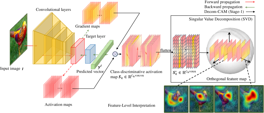
Figure 1: Overview of the decomposition stage of Decom–CAM.

Activation-based Class Activation Map Methods. The activation-based class activation map methods have emerged as an alternative to gradient-based CAM methods to solve the false confidence problem of assigning small channel contributions to large activation values due to the gradient vanishing [18]. Among recent developments, Score-CAM [29] is a notable gradient-free CAM method that employs the activation map as a mask for the input image. The importance of each channel is determined by observing the confidence change of the targeted class when the masked regions are removed, enabling Score-CAM to obtain more reasonable channel contributions. Nevertheless, this approach can be computationally expensive due to each channel requires once forward propagation to obtain its weight, and several variants, such as Score-CAM++ [6], and Group-CAM [33], have been proposed to reduce its computational cost. Although activation-based CAM Methods follow similar paradigms to perturbation-based methods, it derives initial image masks directly from the model’s activation maps, thereby reflecting the model’s internal reasoning process and serving as a valuable complement to gradient-based methods.

2.3 Evaluation of image saliency map.

Deletion and Insertion. The deletion and insertion test [28] is an automatic measuring approach commonly used to evaluate the causal interpretation performance of saliency methods. Specifically, the deletion test quantifies the probability-dropping effect of the target class with the area under the curve (AUC) value when the input image’s pixel is gradually removed based on the importance degree determined by the saliency map. There are several ways of removing the image pixels [7], e.g., setting the pixel values to zero, blurring the pixels, or even cropping out a tight bounding box. A sharp drop of the probability and thus a low ($AUC(Deletion)$) indicates a better interpretation, while the insertion metric measures the increase in probability as pixels are gradually added, with a higher $AUC(Ieletion)$ indicating a better interpretation. And the overall performance in the deletion and insertion test is determined by $AUC(Insertion)-AUC(Deletion)$.

Pointing Game. Pointing game [32] is a popular localization evaluation metric. The localization accuracy of the pointing game test is calculated as the ratio of the number of hits to the total number of hits and misses:

$$ACC=\frac{\#Hits}{\#Hits+\#Misses},$$ (1)

where we count a “hit” when the most salient pixel lies inside the annotated bounding boxes of an object and vice versa. The overall performance is measured by the mean accuracy across all categories in the dataset.

3 Proposed Approach

3.1 Feature-level interpretation with Decom-CAM

Despite the recent success of CAMs in significant regions identification, they have limitations in uncovering finer details of the internal reasoning process, which needs more exploration. As previous work [31] has shown, CNNs can extract distinct levels of features from input images and gradually combine them to form more complex semantic concepts. Thus, by identifying salient features during the model’s inference process, we can provide a finer interpretation of the model’s decision process. The proposed Decom-CAM technique, as shown in Figure 1, employs Singular Value Decomposition and backward gradient to derive multiple class-discriminative Orthogonal Feature Maps from the intermediate activation map of CNNs. By extending these OFMs to the original image size, we can obtain local saliency maps that reveal the salient features upon which CNNs rely to make decisions. As demonstrated in Figure 3, these local saliency maps can accurately identify specific semantic components in the input image, such as the red cross of the medical fleet ship, and the wing of the parrot, thereby extending CAMs’ capabilities to provide a feature-level interpretation of the model prediction. Decom-CAM’s ability to provide finer details of the model’s reasoning process enables us to recognize biases in the model that may have been overlooked by decision-level interpretations and enhance the transparency and credibility of CNNs.

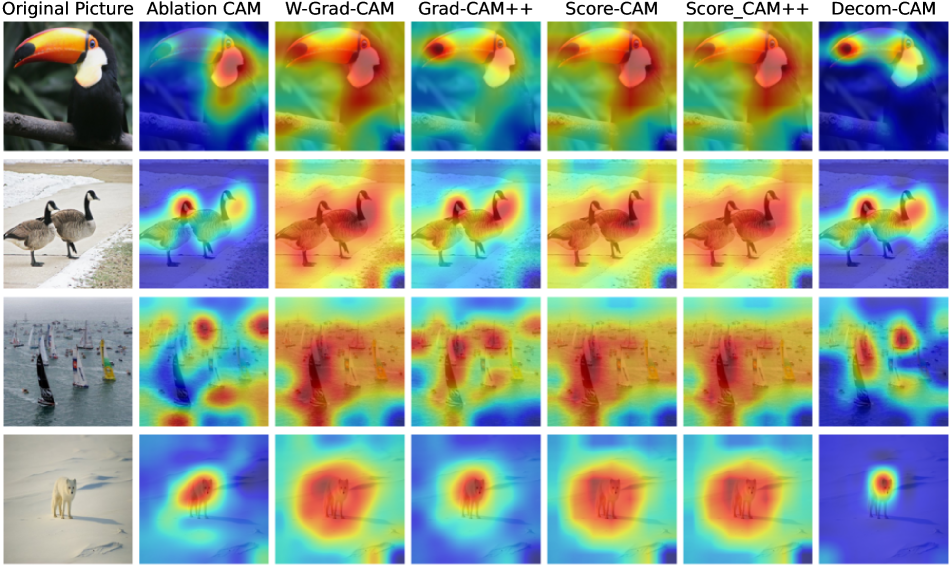
Figure 2: Visualization comparisons of Decom-CAM and currently popular CAM-based saliency map methods on ResNet–50 version of CLIP model. The first column is the input image and the others are saliency maps.

3.2 Decom-CAM

Generally, Decom-CAM in the first stage harnesses SVD to derive multiple OFMs from CNNs’ intermediate activation map to provide feature-level interpretation. In the second stage, Decom-CAM integrates these maps to produce the final decision-level saliency map. Accounting for a few OFMs can contribute to the majority of the variance information of the original feature maps while reducing redundant correlation, Decom-CAM can produce saliency maps swiftly and accurately.

Stage 1–Decomposition Stage. Consider the input image $\bm{I}\in\mathbb{R}^{c_{0}\times h\times w}$ with $c_{0}$ color channels, and a deep convolutional network $\mathcal{F}:\bm{I}\mapsto\bm{y}^{\ell}\in\mathbb{R}^{L}$, where $L$ denotes the total number of classes, and $\ell$ indicates the $\ell^{th}$ coefficient of $\bm{y}$ has the largest confidence value ${y_{\ell}}$. In this stage, our goal is to decompose the intermediate activation maps of the CNN model into multiple orthogonal feature maps that provide feature-level saliency interpretation closely related to the model’s prediction. To achieve this, the orthogonal feature maps should be class-discriminative, and reserve most of the information of the original activation maps. Let $\bm{A}_{k}(\bm{I})$ and $\bm{S}_{k}(\bm{I})$ denote the intermediate activation map of the $k^{th}$ layer in the deep CNN network $\mathcal{F}$ and the class-discriminative activation map, respectively, where $\bm{A}_{k}(\bm{I})\in\mathbb{R}^{c_{k}\times m\times n}$ and $\bm{S}_{k}(\bm{I})\in\mathbb{R}^{c_{k}\times m\times n}$. Henceforth, we ignore the argument $(\bm{I})$ for clarity, unless required. We obtain the class-discriminative activation map by:

$$\bm{S}_{k}=\frac{\partial y_{\ell}}{\partial\bm{A}_{k}}\odot\bm{A}_{k},$$ (2)

where the gradient signal metric $\frac{\partial y_{\ell}}{\partial\bm{A}_{k}}$ contains the contribution of each feature map in $\bm{A}_{k}$ to the final prediction $\ell$, while the Hadamard product symbol $\odot$ highlights the regions activated in both the gradient signal and the original activation map.

In order to extract the salient feature map from $\bm{S}_{k}$, a transformation is first applied to convert $\bm{S}_{k}$ into a two-dimensional matrix denoted as $\bm{S}_{k}^{\ast}\in\mathbb{R}^{c_{k}\times{mn}}$. This is achieved by flattening each feature map in $\bm{S}_{k}$ into a column vector $\bm{S}_{k,i}\in\mathbb{R}^{mn}$. Subsequently, SVD is employed to decompose $\bm{S}_{k}^{\ast}$ into multiple orthogonal feature maps. More specifically, we have the followings:

$$\bm{S}_{k}^{\ast}=\begin{bmatrix}\bm{S}_{k,1}~{}\bm{S}_{k,2}~{}\cdots~{}\bm{S}_{k,c_{k}}\end{bmatrix}.$$ (3)

Then, we perform SVD on $\bm{S}_{k}^{\ast}$ to obtain its decomposition:

$$\bm{S}_{k}^{\ast}=\bm{U}_{k}\bm{\Sigma}_{k}\bm{V}_{k}^{T},$$ (4)

where $\bm{U}_{k}\in\mathbb{R}^{c_{k}\times c_{k}}$ and $\bm{V}_{k}\in\mathbb{R}^{{mn}\times{mn}}$ are unitary matrixes, and $\bm{\Sigma}_{k}\in\mathbb{R}^{c_{k}\times{mn}}$ is a diagonal matrix whose diagonal entries correspond to the singular values of $\bm{S}_{k}^{\ast}$ sorted in descending order. According to the principles of linear algebra, the singular vectors are known to convey a significant proportion of the variance information contained in $\bm{S}_{k}^{\ast}$ [14, 1]. Therefore, we keep singular vectors that correspond to the $\emph{top-}p$ singular values of $\bm{U}_{k}$ to construct a reduced unitary metric denoted as $\bm{U^{\prime}}_{k}\in\mathbb{R}^{c_{k},p}$. Then, we can obtain the channel-wise feature $\bm{F}^{\ast}_{k}\in\mathbb{R}^{p\times mn}$ by projecting $\bm{S}_{k}^{\ast}$ onto a lower-dimensional subspace:

$${\bm{F}_{k}}^{\ast}={\bm{U^{\prime}}_{k}}^{T}{\bm{S}_{k}}^{\ast}.$$ (5)

This process selects the most salient features based on the contribution of each feature map to the total variance and compresses the feature maps by reducing the channel number from $c_{k}$ to $p$.

We can also prove that the different column vectors in $\bm{F}^{\ast}_{k}$ are orthogonal. Denote the singular vectors that correspond to the $\emph{top-}p$ singular values of $\bm{V}_{k}$ as $\bm{V^{\prime}}_{k}\in\mathbb{R}^{mn\times p}$, and the diagonal matrix $\bm{\Sigma^{\prime}}_{k}\in\mathbb{R}^{p\times p}$ whose diagonal entries correspond to the $\emph{top-}p$ singular values sorted in descending order. Specifically, we have:

$${\bm{F}_{k}}^{\ast}={\bm{U^{\prime}}_{k}}^{T}(\bm{U^{\prime}}_{k}\bm{\Sigma^{\prime}}_{k}{\bm{V^{\prime}}_{k}}^{T})=\bm{\Sigma^{\prime}}_{k}{\bm{V^{\prime}}_{k}}^{T},$$ (6)

$${\bm{F}_{k}}^{\ast}{{\bm{F}_{k}}^{\ast}}^{T}=\bm{\Sigma^{\prime}}_{k}({\bm{V^{\prime}}_{k}}^{T}\bm{V^{\prime}}_{k}){\bm{\Sigma^{\prime}}_{k}}^{T}=\bm{\Sigma’}_{k}\odot\bm{\Sigma’}_{k},$$ (7)

where $\bm{V^{\prime}}_{k}$ is a unitary matrix with $\bm{V^{\prime}}_{k}{\bm{V^{\prime}}_{k}}^{T}=\bm{I}$, and $\bm{\Sigma^{\prime}}_{k}$ is a diagonal matrix. Thus, ${\bm{F}_{k}}^{\ast}{{\bm{F}_{k}}^{\ast}}^{T}$ is a diagonal matrix, and the dot product of two different column vectors in $\bm{F}_{k}$ is zero (${{\bm{F}_{k,i}}^{\ast}}^{T}{\bm{F}_{k,j}}^{\ast}=0$) when $i\neq j$. Hence the different column vectors in $\bm{F}_{k}$ are orthogonal, and thereby the salient features help remove the redundant information from the class-discriminative activation maps $\bm{S}_{k}$.

To obtain the final salient feature maps $\bm{F}_{k}\in\mathbb{R}^{p\times m\times n}$, the projected features $\bm{F}^{\ast}_{k}$ are reshaped back into their original spatial dimensions:

$$\bm{F}_{k}=\text{Reshape}(\bm{F}^{\ast}_{k},(p,m,n)).$$ (8)

By reconstructing the feature maps with the retained singular vectors, we effectively remove noisy and redundant information and enhance the discriminative power of the features.

Stage 2–Integrating Stage. In Stage 2, we adopt the activation-based CAM paradigm [29, 6, 33] to generate the final saliency map. Building upon the findings from Stage 1, where we demonstrated the efficacy of retained orthogonal feature maps reserving primary variance information while eliminating redundant correlation from the class-discriminative activation map, we can produce the final saliency map through a few rounds of forward propagation on masked images with interpolated orthogonal feature maps. As a result, the proposed Decom-CAM achieves both precision and computational efficiency in generating the saliency map. We provide a more detailed elaboration on this stage as follows. Firstly, we upsample each orthogonal feature map $F_{k,i}\in\mathbb{R}^{m\times n}$ into the size of the input image to obtain the local saliency map $\bm{H}_{k,i}\in\mathbb{R}^{m\times n}$:

$$\bm{H}_{k,i}=[s\circ Up](F_{k,i}),$$ (9)

where $Up(\cdot)$ denotes the bi-linear interpolation upsampling operation, $s(\cdot)$ denotes a normalization function that maps each element of input matrix into $\begin{bmatrix}0,1\end{bmatrix}$, $[\cdot\circ\cdot]$ denotes the composition of functions.

Next, we create an occluded image $\bm{I}_{m}\otimes\bm{H}_{k,i}\in\mathbb{R}^{c_{0}\times h\times w}$ that is sharp in the region activated by $\bm{H}_{k,i}$ and blurred in the remaining region. Specifically, we first apply Gaussian blur to the original input image $\bm{I}$ to obtain a blurred image $\bm{I}_{b}\in\mathbb{R}^{c_{0}\times h\times w}$, and then obtain the occluded image using the following equation:

$$\bm{I}_{m}^{(i)}\otimes\bm{H}_{k,i}=\text{Max}(\bm{I}_{m}^{(i)}\odot\bm{H}_{k,i},~{}\bm{I}_{b}^{(i)}\odot(1-\bm{H}_{k,i})),$$ (10)

where $\bm{I}_{m}^{(i)}\otimes\bm{H}_{k,i}\in\mathbb{R}^{h\times w}$ denotes the $i^{th}$ channel of the occluded image $\bm{I}_{m}\otimes\bm{H}_{k,i}$, and $\text{Max}(\cdot)$ denotes the element-wise maximum operation.

Then we can calculate the contribution weights $C_{\ell}(F_{k,i})\in\mathbb{R}$ towards the predicted class $\ell$ of each local saliency map $\bm{H}_{k,i}$ as follows:

$$C_{\ell}(F_{k,i})=\mathcal{F}(\bm{I}_{m}\otimes\bm{H}_{k,i})_{\ell}-\mathcal{F}(\bm{I}_{b})_{\ell}.$$ (11)

Finally, we integrate these local saliency maps $\bm{H}_{k,i}$ together to obtain the final saliency map $\mathcal{S}$ as follows:

$$\mathcal{S}=\sum_{i=1}^{p}{\mathcal{A}_{i}\odot\bm{H}_{k,i}},$$ (12)

where $\mathcal{A}$ is a softmax normalization over the contribution weights $\begin{bmatrix}C(F_{k,1})~{}...~{}C(F_{k,p})\end{bmatrix}$ for each local saliency map $\bm{H}_{k,i}$, and $\mathcal{S}$ denotes the final saliency map produced by Decom-CAM.

4 Experiments

4.1 Benchmarks and Baselines

Datasets. In our experiments, we used Mini-ImageNet [27] to measure the interpretability of our methods and the validation set of PASCAL VOC–2012 [9] to assess the locating ability. Mini-ImageNet [27] is a subset of the ImageNet classification dataset with a total of 100 classes, each containing 600 images. We selected the first 100 images of each class, resulting in a benchmark of 10,000 images to measure interpretability. For the locating ability, we used the validation set of PASCAL VOC–2012, which contains 20 classes and 5823 images. All images were resized to 224$\times$224 for testing.

Baselines. Our proposed Decom-CAM method is closely related to CAM-based saliency map methods. Our baselines include gradient-based CAMs (Grad-CAM [25], Grad-CAM++ [4], WGrad-CAM [34], Ablation-CAM [23]) and activation-based CAMs (Score-CAM [29], Score-CAM++ [6]). We conduct all interpretability experiments on a large contrastive language-image pre-training (CLIP) model that trains on four million image-text pairs collected from the internet [21]. We use the ResNet50 version of CLIP and set the target layer to the last convolution layer of CLIP’s stage-4 unless otherwise specified.

Pointing game Metric. The pointing game test has been introduced in the Related work section.

New protocol on Deletion and Insertion Metric. The deletion-insertion test [28] has drawn much attention as a performance evaluation approach for causal interpretability [29, 6, 33, 34], and similar tests measuring Average Drop and Average Increment have been adopted in [23, 4]. However, these assessment approaches fail to consider the correlation between the interpretability performance and the prediction accuracy of the underlying model, where interpretability performance is inherently limited by the model’s decision quality. Additionally, they mix correct and erroneous prediction instances when evaluating the interpretability performance, which is not ideal for comparing different CAM methods.

Thereby, we propose a new protocol based on the deletion-insertion test to solve these limitations. This protocol involves: 1) dividing the test set into multiple subsets based on the model’s performance, using a benchmark accuracy of 10% as the interval criterion for subset creation, which results in 10 distinct subsets that can be evaluated separately to assess the interpretability performance of each saliency method and we can investigate the interpretability performance under distinct model’s prediction performance; 2) excluding the instances that the underlying model makes incorrect predictions. This protocol promises that we can obtain a comprehensive assessment of different CAM methods in a rigorous and appropriate manner.

4.2 Qualitative Analysis

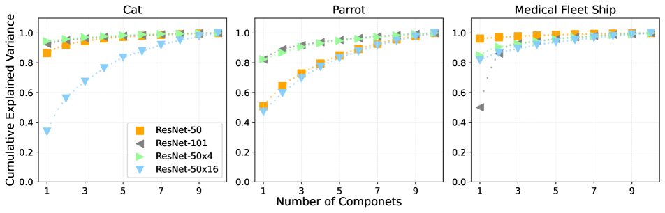
Figure 3: Comparisons of the local saliency maps (orthogonal feature maps) with different backbones. The upper subfigure visualizes the components corresponding to the top-3 singular values of different versions of CLIP, with each row representing a distinct backbone. Meanwhile, the lower subfigure showcases the cumulative explained variance curve of the SVD decomposition results of various models on the last three images in the upper subfigure.

Visualization of the orthogonal feature maps. Here we present a detailed visualization of the orthogonal feature maps (OFMs) for various versions of the CLIP model, namely, ResNet-50, ResNet-101, ResNet-50$\times$4, and ResNet-50$\times$16. Consistent with the general paradigm of CAM techniques, we extrapolate the OFMs to the input image size to obtain feature-level local saliency maps. The upper subfigure of Figure 3 displays the OFMs corresponding to the top-3 singular values, which reveal the salient features that the model relies on to make decisions, e.g., the ear in the cat image and the red cross in the medical fleet ship image. Additionally, the lower subfigure of Figure 3 demonstrates the cumulative explained variance curves of the singular values obtained by SVD on the class-discriminative activation map for different versions of the CLIP model. Our results indicate that we can capture most of the variance information in the original activation map with only a few OFMs, which aligns with our argument that a few OFMs can spotlight the salient features found by the model. Notably, we observed that a larger model does not necessarily result in better interpretable features. Specifically, the local saliency map of ResNet-50$\times$16 occasionally contains significant noise (shown in the last column of the upper subfigure of Figure 3), indicating that increasing the model size may not always enhance its interpretability. Overall, our results illustrate the effectiveness of OFMs in capturing salient features across various versions of the CLIP model [21].

Comparison with Different Saliency Methods. Here we present a comparison between Decom-CAM and several other saliency methods in terms of their visualization performances. As shown in Figure 3.1, Decom-CAM effectively overcomes the noise issue commonly encountered in gradient-based approaches. Moreover, Decom-CAM provides more precise object localization compared to activation-based methods. Notably, as shown in the fourth row of Figure 3.1, when dealing with tiny objects, our method achieves an exceptional level of refinement that was previously unattainable by existing techniques. These results demonstrate the proposed Decom-CAM generates high-quality and fine-grained interpretation for various types of input images.

4.3 Quantitative Analysis

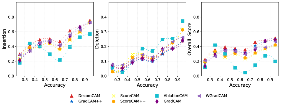
Figure 4: The experimental results were obtained by utilizing the proposed protocol on the deletion and insertion metric, which demonstrates the relationship between the interpretability methods’ performance and the model’s prediction accuracy. The x-axis of the plot represents the model’s performance on specific data subsets, categorized by intervals of 10%, whereas the y-axis denotes the corresponding interpretability methods’ scores on the respective metrics.

Pointing Game on VOC2012. The experimental results on the Pointing Game [32] test, as presented in Table 1, suggest that the Decom-CAM method has demonstrated superior performance over all other baselines, and Grad-CAM++ is a close second. The results indicate that Decom-CAM has surpassed alternative techniques by more than 1.16% in terms of pointing game accuracy. This is mainly due to Decom-CAM’s detailed and finely-grained saliency map that can accurately locate the target class to interpret.

New Protocol in Deletion and Insertion Task. Here we present the experimental results of our proposed evaluation protocol, which are depicted in Figure 4. Each CAM method is represented by a curve that illustrates how its interpretation performance changes with respect to the model’s prediction accuracy on the specific sub-testset. To provide an overall assessment of the models, we calculate the area under the curve (AUC) for each curve. Table 2 collects the AUC score of the Deletion and Insertion curve under the proposed protocol, where Decom-CAM outperforms all other methods in terms of the insertion ($4.49\%\uparrow$) and overall score metrics ($3.33\%\uparrow$). Regarding the Deletion metric, we attribute the better performance of Grad-CAM++ to its broader saliency maps that tend to cover larger regions, as shown in Figure 3.1. Nonetheless, this comes at the cost of not being able to accurately locate the most salient areas when calculating the insertion metric. From the Overall Score perspective, Decom-CAM outperforms all other methods and achieves the state-of-the-art performance. Besides, Figure 4 demonstrates the superiority of the proposed Decom-CAM over current state-of-the-art methods in generating precise saliency maps across all levels of classification accuracy.

Moreover, an important finding of our study is that the discrepancies in the insertion metrics among various interpretability methods reduce and converge to zero as the model’s performance improves. This observation has practical implications, as it suggests that the interpretability methods become more valuable when the model’s performance is poor. In such situations, understanding the model’s decision-making process can provide critical insights to enhance its performance. Our results indicate that the selection of interpretability methods is particularly crucial for models with lower accuracy, but it may become less critical for highly accurate models.

Method	Accuracy(%)$\uparrow$
GradCAM	82.85
GradCAM++	85.70
WGradCAM	72.99
ScoreCAM	67.25
ScoreCAM++	66.53
AblationCAM	48.31
Decom-CAM	86.86

Table 1: Pointing game test in VOC2012 validation set.

Method	Insertion(%) $\uparrow$	Deletion(%)$\downarrow$	Overall Score(%)$\uparrow$
GradCAM	47.56	12.80	34.76
GradCAM++	48.18	11.71	36.47
WGradCAM	48.22	14.83	33.39
ScoreCAM	44.54	15.13	29.41
ScoreCAM++	45.19	14.51	30.68
AblationCAM	37.78	17.03	20.75
Decom-CAM	52.67	12.87	39.80

Table 2: The AUC score of the Deletion and Insertion curve under the proposed protocol.

5 Conclusion

This paper introduces a novel deep learning interpretation method, named Decomposition Class Activation Map (Decom-CAM). Unlike other CAM methods that focus on object localization, our method can identify salient features closely related to the model’s decision. To achieve this, we first decompose intermediate activation maps of convolution layers into orthogonal features using the SVD operation and integrate them to generate fine-grained saliency maps. The orthogonality of features enables Decom-CAM to capture local features, making it more beneficial for deep model interpretation. We identify previous evaluation approaches’ oversight on the correlation between interpretability performance and model prediction accuracy and introduce a new protocol that divides datasets into subsets according to classification performance to evaluate different interpretability methods appropriately and rigorously. Our experiments show that discrepancies in insertion metrics among various interpretability methods reduce and converge to zero as model performance improves, emphasizing the selection of interpretability methods’ importance for lower-accuracy models. Additionally, we demonstrate how our new protocol can provide a more comprehensive evaluation of saliency methods by showing the curve that interpretability performance changes with respect to the model’s prediction accuracy. We hope that our feature-level interpretation and evaluation protocol will inspire future research in this direction.

References

- [1] Hervé Abdi and Lynne J Williams. Principal component analysis. Wiley interdisciplinary reviews: computational statistics, 2(4):433–459, 2010.
- [2] Ayoub Benali Amjoud and Mustapha Amrouch. Convolutional neural networks backbones for object detection. In Proceedings of Image and Signal Processing, pages 282–289, 2020.
- [3] Lennart Brocki and Neo Christopher Chung. Evaluation of interpretability methods and perturbation artifacts in deep neural networks. arXiv preprint arXiv:2203.02928, 2022.
- [4] Aditya Chattopadhay, Anirban Sarkar, Prantik Howlader, and Vineeth N Balasubramanian. Grad-CAM++: Generalized gradient-based visual explanations for deep convolutional networks. In Proceedings of IEEE winter conference on applications of computer vision, pages 839–847. IEEE, 2018.
- [5] Sheng Chen, Yang Liu, Xiang Gao, and Zhen Han. Mobilefacenets: Efficient cnns for accurate real-time face verification on mobile devices. In Chinese Conference of Biometric Recognition (CCBR), pages 428–438, 2018.
- [6] Yifan Chen and Guoqiang Zhong. Score-CAM++: Class discriminative localization with feature map selection. In Journal of Physics: Conference Series, volume 2278, page 012018, 2022.
- [7] Piotr Dabkowski and Yarin Gal. Real time image saliency for black box classifiers. Advances in neural information processing systems, 30, 2017.
- [8] Filip Karlo Došilović, Mario Brčić, and Nikica Hlupić. Explainable artificial intelligence: A survey. In International convention on information and communication technology, electronics and microelectronics (MIPRO), pages 210–215, 2018.
- [9] Mark Everingham, Luc Van Gool, Christopher KI Williams, John Winn, and Andrew Zisserman. The pascal visual object classes (voc) challenge. International journal of computer vision, 88:303–308, 2009.
- [10] Ruth Fong, Mandela Patrick, and Andrea Vedaldi. Understanding deep networks via extremal perturbations and smooth masks. In Proceedings of the IEEE/CVF international conference on computer vision, pages 2950–2958, 2019.
- [11] Ruth C Fong and Andrea Vedaldi. Interpretable explanations of black boxes by meaningful perturbation. In Proceedings of the IEEE international conference on computer vision, pages 3429–3437, 2017.
- [12] Ross Girshick, Jeff Donahue, Trevor Darrell, and Jitendra Malik. Rich feature hierarchies for accurate object detection and semantic segmentation. In Proceedings of the IEEE conference on computer vision and pattern recognition, pages 580–587, 2014.
- [13] Kaiming He, Xiangyu Zhang, Shaoqing Ren, and Jian Sun. Deep residual learning for image recognition. In Proceedings of the IEEE conference on computer vision and pattern recognition, pages 770–778, 2016.
- [14] Roger A Horn and Charles R Johnson. Matrix analysis. Cambridge university press, 2012.
- [15] Maksims Ivanovs, Roberts Kadikis, and Kaspars Ozols. Perturbation-based methods for explaining deep neural networks: A survey. Pattern Recognition Letters, 150:228–234, 2021.
- [16] Mohammad AAK Jalwana, Naveed Akhtar, Mohammed Bennamoun, and Ajmal Mian. CAMERAS: Enhanced resolution and sanity preserving class activation mapping for image saliency. In Proceedings of the IEEE Conference on Computer Vision and Pattern Recognition, pages 16327–16336, 2021.
- [17] Peng-Tao Jiang, Chang-Bin Zhang, Qibin Hou, Ming-Ming Cheng, and Yunchao Wei. Layer-CAM: Exploring hierarchical class activation maps for localization. IEEE Transactions on Image Processing, 30:5875–5888, 2021.
- [18] Hyungsik Jung and Youngrock Oh. Towards better explanations of class activation mapping. In Proceedings of the IEEE International Conference on Computer Vision, pages 1336–1344, 2021.
- [19] Zachary C. Lipton. The mythos of model interpretability. Communications of the ACM, 61(10), 2018.
- [20] Tim Miller. Explanation in artificial intelligence: Insights from the social sciences. Artificial intelligence, 267:1–38, 2019.
- [21] Alec Radford, Jong Wook Kim, Chris Hallacy, Aditya Ramesh, Gabriel Goh, Sandhini Agarwal, Girish Sastry, Amanda Askell, Pamela Mishkin, Jack Clark, et al. Learning transferable visual models from natural language supervision. In International conference on machine learning, pages 8748–8763. PMLR, 2021.
- [22] Sylvestre-Alvise Rebuffi, Ruth Fong, Xu Ji, and Andrea Vedaldi. There and back again: Revisiting backpropagation saliency methods. In Proceedings of the IEEE Conference on Computer Vision and Pattern Recognition, pages 8839–8848, 2020.
- [23] Desai S. and Ramaswamy H. G. Ablation-CAM: Visual explanations for deep convolutional network via gradient-free localization. In Proceedings of the IEEE Winter Conference on Applications of Computer Vision, pages 983–991, 2020.
- [24] Zaid Saeb Sabri and Zhiyong Li. Low-cost intelligent surveillance system based on fast cnn. PeerJ Computer Science, 7:e402, 2021.
- [25] Ramprasaath R Selvaraju, Michael Cogswell, Abhishek Das, Ramakrishna Vedantam, Devi Parikh, and Dhruv Batra. Grad-CAM: Visual explanations from deep networks via gradient-based localization. In Proceedings of the IEEE international conference on computer vision, pages 618–626, 2017.
- [26] Karen Simonyan, Andrea Vedaldi, and Andrew Zisserman. Deep inside convolutional networks: Visualising image classification models and saliency maps. arXiv preprint arXiv:1312.6034, 2013.
- [27] Oriol Vinyals, Charles Blundell, Timothy Lillicrap, Daan Wierstra, et al. Matching networks for one shot learning. Advances in neural information processing systems, 29, 2016.
- [28] Petsiuk Vitali, Das Abir, and Saenko Kate. RISE: Randomized input sampling for explanation of black-box models. In Proceedings of British Machine Vision Conference, page 151, 2018.
- [29] Haofan Wang, Zifan Wang, Mengnan Du, Fan Yang, Zijian Zhang, Sirui Ding, Piotr Mardziel, and Xia Hu. Score-CAM: Score-weighted visual explanations for convolutional neural networks. In Proceedings of the IEEE conference on computer vision and pattern recognition workshops, pages 24–25, 2020.
- [30] Qing Yang, Xia Zhu, Jong-Kae Fwu, Yun Ye, Ganmei You, and Yuan Zhu. Mfpp: Morphological fragmental perturbation pyramid for black-box model explanations. In Proceedings of the International conference on pattern recognition, pages 1376–1383, 2021.
- [31] Matthew D Zeiler and Rob Fergus. Visualizing and understanding convolutional networks. In Proceedings of European Conference on Computer Vision, pages 818–833, 2014.
- [32] Jianming Zhang, Sarah Adel Bargal, Zhe Lin, Jonathan Brandt, Xiaohui Shen, and Stan Sclaroff. Top-down neural attention by excitation backprop. International Journal of Computer Vision, 126(10):1084–1102, 2018.
- [33] Qinglong Zhang, Lu Rao, and Yubin Yang. Group-CAM: Group score-weighted visual explanations for deep convolutional networks. arXiv preprint arXiv:2103.13859, 2021.
- [34] Qinglong Zhang, Lu Rao, and Yubin Yang. A novel visual interpretability for deep neural networks by optimizing activation maps with perturbation. In Proceedings of the AAAI Conference on Artificial Intelligence, volume 35, pages 3377–3384, 2021.
- [35] Bolei Zhou, Aditya Khosla, Agata Lapedriza, Aude Oliva, and Antonio Torralba. Learning deep features for discriminative localization. In Proceedings of the IEEE conference on computer vision and pattern recognition, pages 2921–2929, 2016.