ModuleFormer:
Modularity Emerges from Mixture-of-Experts

Abstract

Large Language Models (LLMs) have achieved remarkable results. But existing models are expensive to train and deploy, and it is also difficult to expand their knowledge beyond pre-training data without forgetting previous knowledge. This paper proposes a new neural network architecture, ModuleFormer, that leverages modularity to improve the efficiency and flexibility of large language models. ModuleFormer is based on the Sparse Mixture of Experts (SMoE). Unlike previous SMoE-based modular language model (Gururangan et al., 2021), which requires domain-labeled data to learn domain-specific experts, ModuleFormer can induce modularity from uncurated data with its new load balancing and load concentration losses. ModuleFormer is a modular architecture that includes two different types of modules, new stick-breaking attention heads, and feedforward experts. Different modules are sparsely activated conditions on the input token during training and inference. In our experiment, we found that the modular architecture enables three important abilities for large pre-trained language models: 1) Efficiency, since ModuleFormer only activates a subset of its modules for each input token, thus it could achieve the same performance as dense LLMs with more than two times throughput; 2) Extendability, ModuleFormer is more immune to catastrophic forgetting than dense LLMs and can be easily extended with new modules to learn new knowledge that is not included in the training data; 3) Specialisation, finetuning ModuleFormer could specialize a subset of modules to the finetuning task, and the task-unrelated modules could be easily pruned for a lightweight deployment. The inference code and model weights are here: https://github.com/IBM/ModuleFormer.

1 Introduction

While modern Large Language Models (LLMs) have achieved remarkable results and even surpassed human performance on some tasks, it remains inefficient and inflexible. Most LLMs (e.g. Llama, Touvron et al. 2023; Pythia, Biderman et al. 2023; GPT-3, Brown et al. 2020) use all of their parameters during inference and training. We refer to these as dense models. However, previous work has shown that, a large portion of parameters in a neural model can be pruned while still maintaining similar performance (Frankle and Carbin, 2018; Frantar and Alistarh, 2023; LeCun et al., 1989). Furthermore, LLMs are ‘frozen in time’ once trained, but many practical use cases require the LLMs to have up-to-date knowledge (Lazaridou et al., 2022).

Furthermore, fine-tuning the entire model for domain adaptation or continual learning is becoming costly and compute-prohibitive as model sizes grow, making it infeasible for users with smaller computational budgets. Updating all parameters also makes the model vulnerable to catastrophic forgetting (McCloskey and Cohen, 1989; Aghajanyan et al., 2021). To this end, lightweight adaptation methods like LoRA that update only a small subset of the original parameters are becoming popular (Hu et al., 2021; Samarakoon and Sim, 2016). However, our experiments show that such methods can still suffer catastrophic forgetting and are less capable of adapting to a substantially different domain, like a new language.

Modularity could be a good solution for LLMs to address the aforementioned issues. A modular model could have several benefits: 1) the model could activate a subset of module conditions on the input or task, thus using less computation than densely activating the entire model; 2) given a domain or task, a subset of domain/task-related modules could be assembled to form a new lightweight model; 3) the model could be easily extended with new modules for domain adaption or continual learning; 4) the model could be more immune to catastrophic forgetting because only the input-related modules are updated during the model fine-tuning.

The notion of neural network modules is not new. Andreas et al. (2016) proposes Neural Module Networks (NMN) for visual question-answering tasks. NMN has limited practicality because it requires intensive domain knowledge to assign a predefined functionality for each neural module and combines these modules with respect to the internal structure of the input question. DEMix (Gururangan et al., 2021) and Mod-Squad (Chen et al., 2022) propose to leverage Sparse Mixture of Experts [SMoEs, Shazeer et al. 2017] to combine modularity with the Transformer architecture. While experts in SMoE are similar to the modules in NMN, the drawback of SMoE is the lack of established methods to manipulate experts, including selecting experts for a specific task and adding new experts for domain adaptation. To solve this problem, DEMix and Mod-Squad use curated training data to learn the functionality of each expert. However, curated data is always hard to obtain and scale up.

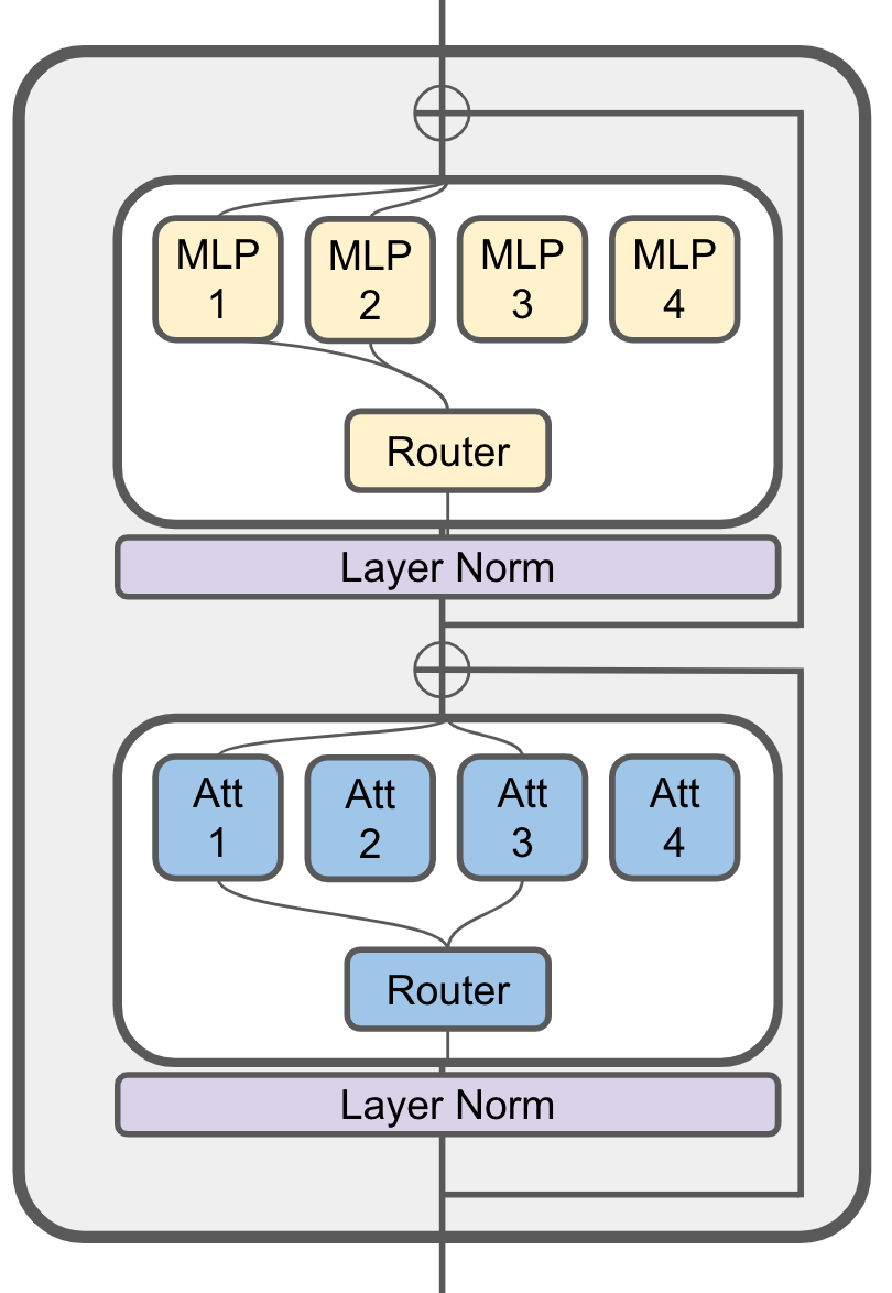
(a) Sparse activation of modules

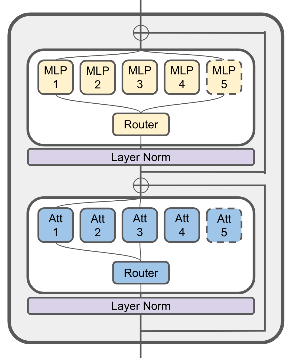
(b) Adding new modules

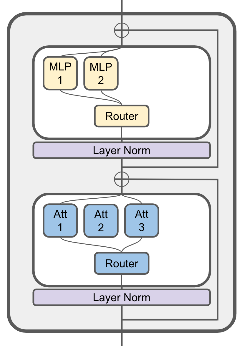
(c) Pruning modules

Figure 1: The architecture of ModuleFormer. The sparse activation schema enables high computation efficiency. Adding new modules is simply inserting randomly initialized ones into each layer and then training the new experts and the router on a new dataset. The number and size of new modules can be customized to accommodate different scenarios. Pruning modules involves counting the activation frequency of each module and setting a threshold to remove the least used modules. The percentage of prune could also be customized to achieve a trade of between performance and model size.

This paper argues that modularity can emerge from language model pretraining with uncurated data. We propose a new modular architecture, ModuleFormer (Fig. 1(a)), and the associated methods for module manipulation. ModuleFormer comprises FFD modules and a novel stick-breaking attention mechanism, and a new mutual information loss that balances the load of different modules. Furthermore, we demonstrate inserting new modules (Fig. 1(b)), and expert pruning (Fig. 1(c)) can be done in ModuleFormer. To enable pruning, we introduce a new load concentration loss to select and specialize a subset of modules on a given task. Our experiment result shows the promising abilities of ModuleFormer: 1) It achieves the same performance as dense LLMs with lower latency (50%) and a smaller memory footprint; thus, it could process more than 2 times the number of tokens per second; 2) It is less susceptible to catastrophic forgetting after finetuning the entire model on a new domain, and it could also be easily extended with new modules to learn a new language; 3) It can be finetuned on a downstream task to specialize a subset of modules on the task and the unused modules can be pruned without sacrificing performance.

2 Related Work

Pretrained Language Models and finetuning. Pretraining is crucial for attaining good results on NLP tasks. In previous transfer-learning regimes, the de facto standard was to finetune a pretrained model on a downstream task, updating all its parameters (Devlin et al., 2018). With the increasing scale of language models (Radford et al., 2019; Brown et al., 2020; Chowdhery et al., 2022), this procedure has become increasingly difficult for researchers without similar computing resources to the research groups that trained them. As a result, prompting and prompt engineering became the go-to method for NLP researchers to leverage the capabilities of these LLMs to solve their task (Brown et al., 2020). Alternatively, methods that adapt only a subset of parameters grew in popularity (Houlsby et al., 2019; Rebuffi et al., 2017; Lin et al., 2020). Low-rank adaptation (LoRA, Hu et al. 2021) is a popular method being used in a wide variety of models. We show that LoRA, while effective for small adaptations to LLMs for specific tasks, fail to perform as well if tasked to learn a different language.

Sparse Mixture of Experts for Modularity SMoE methods for sparse conditional computation was introduced in Shazeer et al. (2017), primarily with the goal of scaling up models. Fedus et al. (2021) used this property to great effect to train the Switch Transformer, sharding the different experts to different compute nodes to fully leverage distributed training regimes. Our goal, however, is to leverage SMoEs for the purpose of modularity. The notion of modularity in neural models is not new. Previous works have proposed several ways to introduce modularity to neural network models. Andreas et al. (2016) introduces the Neural Module Network (NMN) for visual question-answering tasks. An NMN is composed of several predefined neural network modules. Each module has a clear definition of its functionality. These modules are dynamically assembled for different instances of a reasoning task. But NMN requires highly curated data with expert labels, and the number of predefined modules is task-specific, thus limiting its application to other tasks.

DEMix (Gururangan et al., 2021) combines the SMoE with modular schema. It proposes to train different feedforward experts for different domains, with each feedforward expert functioning as a module with specific domain knowledge. However, DEMix is pretrained on curated data with domain labels, whereas the state-of-the-art LLMs are trained on large-scale domain-agnostic data. Furthermore, when the input domain is unknown, the inference cost of Demix linearly increases with the number of modules.

Length-extrapolation in Attention Position embeddings introduced in Vaswani et al. (2017) used sinusoidal embeddings to represent positions in the sentence. This should allow the key-query interactions to extrapolate to positions unseen during training, but this is unfortunately not the case in practice (Press et al., 2021). Efforts have been made to improve the extrapolation capabilities of position embeddings (Su et al., 2021; Sun et al., 2022).

In ModuleFormer, we encode positional information without positional embeddings. Our method can be considered as a simplification of Geometric Attention (Csordás et al., 2021). This formulation, also known as stick-breaking after this formulation of the Dirichlet process, has been used in different settings in deep learning (Dehghani et al., 2018; Banino et al., 2021; Graves, 2016; Tan and Sim, 2016). While ALiBi (Press et al., 2021) also biases toward recent time steps, ALiBi can inhibit attending on terms further away, as the positional bias overwhelms the content attention scores, whereas stick-breaking attention does not have the same issue.

Continual Learning Prior work has demonstrated the advantages of continual learning (Alsentzer et al., 2019; Chakrabarty et al., 2019; Lee et al., 2020; Beltagy et al., 2019) . When data that was previously used in training is available, joint training (Caruana, 1997) is known to be the most straightforward method with the best performance (Li and Hoiem, 2017). For lifelong learning (i.e. previously trained data is not available), the newly trained network tends to forget knowledge learned in the previously trained tasks. This is known as catastrophic forgetting (McCloskey and Cohen, 1989). To overcome this phenomenon, Kirkpatrick et al. (2017) proposed a regularization method. Munkhdalai and Yu (2017); Beaulieu et al. (2020) learns to perform lifelong learning through meta-learning. These approaches are orthogonal to methods like DEMix-dapt (Gururangan et al., 2021) and ModuleFormer, and can be combined with these methods. However, DEMix-dapt belongs to the duplicated and fine-tuned category in the taxonomy introduced by Li and Hoiem (2017), where a model is duplicated several times for each task. This causes great inconvenience when performing inference on domain-agnostic data.

Neural Network Pruning Neural Network Pruning eliminates redundant parameters and structure to accelerate inference in neural networks. Previous work has focused more on structured model pruning (Li et al., 2016; He et al., 2017). These pruned models often benefit from additional finetuning to achieve improved performance. However, other recent work show that compressed models can be trained from scratch to achieve comparable performance, eliminating the need for the reliance on fine-tuning (Liu et al., 2018; Wang et al., 2020). One way pruning is simplified in SMoE-based models is to prune off entire experts, without significantly changing model architecture. However, previous SMoE-based large language models (Shazeer et al., 2017; Lepikhin et al., 2020; Fedus et al., 2021) have been trained with load balancing losses which forces the model to use every expert. As a result, pruning experts is more likely to lead to sacrifices in performance. We propose the load concentration loss that biases the model towards using fewer modules during adaptation or finetuning to alleviate this problem.

3 Model Architecture

3.1 Preliminary: Mixture of Experts

A Mixture of Experts (MoE) layer comprises $N$ modules $f_{1},\ldots,f_{N}$ and a router $g(m\mid\mathbf{x})$. Given an input $\mathbf{x}$ to the MoE layer, the router predicts a probability distribution over the $N$ modules. Of these, we select the top $k$ experts. When $k<N$ , we are using a Sparse Mixture of Experts (SMoE, Shazeer et al. 2017). In this paper, we use an MLP to model the router

$$g(m\mid\mathbf{x}) =\text{Top}k\left(\frac{e^{h(\mathbf{x})_{i}}}{\sum e^{h(\mathbf{x})_{j}}}\right),$$ (1)

$$h(\mathbf{x}) =\mathbf{A}\ \mathrm{ReLU}(\mathbf{B}\mathbf{x}),$$ (2)

where $h(\mathbf{x})$ is modeled by an MLP, $\mathbf{A}$ is the expert embedding matrix of shape $(N,D_{\text{rtr}})$, $\mathbf{B}$ is the input projection matrix of shape $(D_{\text{rtr}},D_{\text{emb}})$, $\text{Top}k$ is the operator that sets all gates to zero except the top $k$ gates. The final output of the SMoE is then given by $y=\sum_{m=1}^{N}g(m\mid\mathbf{x})\cdot f_{m}(\mathbf{x})$. When $g(m\mid\mathbf{x})=0$, $f_{m}(\mathbf{x})$ will not need to be evaluated, thus reducing computation cost during training and inference.

Compared to a standard transformer decoder block, a ModuleFormer block replaces the Feed-forward layer (FFD) with a SMoE layer and the self-attention layer with a Mixture of Attention heads (MoA) layer inspired by Zhang et al. (2022). Each SMoE layer can be described by a 3-tuple, $(N_{\mathrm{ffd}},k,D_{\mathrm{ffd}})$, with $N_{\mathrm{ffd}}$ as the number of FFD modules, $k$ is the parameter in the top-$k$ operation, and $D_{\mathrm{ffd}}$ is the dimension of the hidden layer inside each module. Like the MoE layer, an MoA layer has $N_{\mathrm{att}}$ attention modules and activates the top-$k$ modules for each input. Unlike Zhang et al. (2022), we introduce a new stick-breaking self-attention module.

3.2 Stick-breaking Self-Attention head

The stick-breaking self-attention is designed for the Transformer decoder to model the attention of each token $\mathbf{x}_{t}$ to previous tokens $\mathbf{x}_{<t}$. It uses the stick-breaking process view of the Dirichlet process to model the attention distribution instead of the softmax in a standard attention layer. The motivation to pay attention to the latest matching tokens. It can also be considered a simplification of the geometric attention proposed in Csordás et al. (2021).

Given an input vector sequence of $t$ time steps $\mathbf{x}_{1},\mathbf{x}_{2},...,\mathbf{x}_{t}$, each input is projected to a sequence of key vectors $\mathbf{k}_{1},\mathbf{k}_{2},...,\mathbf{k}_{t}$ and a sequence of value vectors $\mathbf{v}_{1},\mathbf{v}_{2},...,\mathbf{v}_{t}$. To compute the attention of time step $t$, the input $\mathbf{x}_{t}$ is projected to a query vector $\mathbf{q}_{t}=\mathbf{W}_{q}\mathbf{x}_{t}$, where $\mathbf{W}_{q}$ is the query projection matrix. For all previous steps and the current step $i\leq t$, we compute the probability that the key at time step $i$ matches the query at time step $t$:

$$\beta_{i,t}=\mathrm{sigmoid}(\mathbf{k}_{i}^{\mathsf{T}}\mathbf{q}_{t}).$$ (3)

To get the attention weights of the most recent matching key, we use the stick-breaking process:

$$p_{i,t}=\beta_{i,t}\prod_{i<j\leq t}\left(1-\beta_{j,t}\right).$$ (4)

Note that $\sum_{i}p_{i,t}\leq 1$, and sums to 1 given a sufficiently long context (See Appendix A). Further, as in Csordás et al. (2021), this can be efficiently computed with a combination of cumulative sums in log-space. Based on the attention distribution $p_{i,t}$, we can compute the attention output as:

$$\mathbf{o}_{t}=\mathbf{W}_{o}^{\mathsf{T}}\sum_{i\leq t}p_{i,t}\mathbf{v}_{i},$$ (5)

where $\mathbf{W}_{o}$ is the output projection matrix.

Since Equation 4 selects the latest match token, the stick-breaking attention implicitly encodes position information, negating the need for explicit modeling of position with sinusoidal embeddings or relative position biases, and drastically simplifies length-extrapolation of self-attention. After pre-training on a fixed input length, the model could theoretically process any input length. Like Dai et al. (2019), we also concatenate the key and value from the previous batch to the current batch during pre-training, extending the effective context length from sequence length $T$ to $N_{L}T$, where $N_{L}$ is the number of ModuleFormer Blocks.

As in Zhang et al. (2022), each stick-breaking self-attention head is composed of four $\mathbb{R}^{D_{emb}\times D_{att}}$ matrix $\mathbf{W}_{q},\mathbf{W}_{k},\mathbf{W}_{v},\mathbf{W}_{o}$, where $D_{att}$ is the attention head dimension, $\mathbf{W}_{k}$ and $\mathbf{W}_{v}$ are shared by different heads, $\mathbf{W}_{q}$ and $\mathbf{W}_{o}$ are different across heads. In the case of $D_{att}$ equal to $D_{emb}$, we can set $\mathbf{W}_{k}$ and $\mathbf{W}_{v}$ to the identity matrix to eliminate the shared parameters between heads.

4 Module Manipulation

4.1 Load Balancing during Pretraining

To avoid the SMOEs repeatedly using the same module and wasting the extra capacity in the other modules, it requires various load balancing losses to regulate the training of the router (Shazeer et al., 2017; Fedus et al., 2021). Mod-Squad (Chen et al., 2022) proposes to maximize the Mutual Information between modules and tasks to balance the load of different experts and build alignment between tasks and experts.

Unlike Chen et al. (2022), we want to maximize the Mutual Information (MI) between tokens and modules:

$$\mathcal{L}_{\text{MI}}=\sum_{\mathbf{x}}\sum_{m}p(m,\mathbf{x})\log\left(\frac{p(m,\mathbf{x})}{p(m)p(\mathbf{x})}\right).$$ (6)

We assume for simplicity that $\mathbf{x}$ is uniform over the set of $\mathbf{x}$ in the batch, $\mathcal{X}$, and therefore $p(\mathbf{x})=\frac{1}{\mathcal{X}}$. After removing all constant components, we can simplify the MI loss to be the difference between the entropy of $p(m)$ and the conditional entropy of $p(m\mid\mathbf{x})$:

$$\mathcal{L}_{\text{MI}}=\underbrace{\sum_{m=1}^{N}p(m)\log p(m)}_{-H(m)}-\frac{1}{|\mathcal{X}|}\sum_{\mathbf{x}\in\mathcal{X}}\underbrace{\sum_{m=1}^{N}g(m\mid\mathbf{x})\log g(m\mid\mathbf{x})}_{H(m\mid\mathbf{x})},$$ (7)

where $p(m)=\sum_{\mathbf{x}}g(m|\mathbf{x})p(\mathbf{x})$, $p(\mathbf{x})$ is the probability of each token inside the batch, $H(m)$ is the entropy of modules’ marginal distribution, $H(m\mid\mathbf{x})$ is the entropy the modules’ probability condition on input $\mathbf{x}$, $|\mathcal{X}|$ is the number of tokens. For a minibatch of size $B$ with length $T$, the number of tokens is $|\mathcal{X}|=BT$, and the token probability is $p(x)=1/|\mathcal{X}|$. Intuitively, the MI loss maximizes the entropy of modules’ marginal distribution and minimizes the entropy of the conditional distribution of modules given an input $\mathbf{x}$. It balances the load of each expert across the entire batch (maximize $H(m)$), but also encourages each input $\mathbf{x}$ to concentrate their gating probability to fewer modules (minimize $H(m\mid\mathbf{x})$).

4.2 Load Concentration during Finetuning

While we want to maximize the use of each expert during pretraining, we want to hone in on the modules used for specific downstream tasks. This way, we can remove unused modules and reduce the number of parameters for the finetuned model. To concentrate the load on fewer experts, we minimize the marginal entropy instead,

$$\mathcal{L}_{\text{entropy}}=H(m)=-\sum_{m=1}^{N}p(m)\log p(m),$$ (8)

encouraging the model to use fewer experts. After fine-tuning, we can count the module frequency $f_{m}$ used on the training or validation sets. The $f_{m}$ represents the importance of module $m$ for this task. We can easily prune the model by removing experts with $f_{m}$ less than a certain threshold. Appendix D.2 demonstrates the benefits of load concentration when finetuning.

4.3 Inserting new Modules for Continual Learning

For modularized models, inserting new modules is a straightforward and parameter-efficient method to learn new knowledge without fine-tuning the entire model. When inserting $N_{new}$ randomly initialized modules to each layer, we also extend the module embedding layer $\mathbf{A}$ in the router (Eq. 2) with a new matrix $\mathbf{A}^{\prime}$ of shape $(N_{new},D_{\text{rtr}})$. Hence the new routing function can be written as:

$$h^{\prime}(\mathbf{x})=\begin{bmatrix}\mathbf{A}\\ \mathbf{A}^{\prime}\end{bmatrix}\ \mathrm{ReLU}(\mathbf{B}\mathbf{x}).$$ (9)

Since the parameters in previous modules are frozen during fine-tuning, continual learning with new modules could largely avoid the catastrophic forgetting problem. However, catastrophic forgetting could still happen to the router. This occurs when new modules are trained on a new domain, and the router erroneously routes input from the old domain to the new expert.

To avoid this issue, we make the router partially trainable and apply regularization. In detail, we freeze $\mathbf{A}$ and $\mathbf{B}$, leaving only $\mathbf{A}^{\prime}$ trainable. Furthermore, we introduce a technique called ’routing regularization’, which restricts the norm of $\mathbf{A}^{\prime}$:

$$\mathcal{L}_{\mathrm{rout\_reg}}=\big{|}\big{|}\mathbf{A}^{\prime}\big{|}\big{|}^{2}.$$ (10)

This method effectively limits the usage of new experts, as a larger magnitude of $\mathbf{A}^{\prime}$ corresponds to a higher probability of the new experts being prioritized.

Unlike classical regularization approaches for continual learning, such as decay or L2 Loss, which have been pointed out to be defective (Lesort et al., 2019), our routing regularization doesn’t restrict the capacity of experts but only restricts the tendency of usage of new experts. Appendix C.5 demonstrates the benefits of the partially trainable router and routing regularization.

5 Experiments

5.1 Language Modeling

Table 1: Language Model Hyperparameters

Model	$D_{\text{emb}}$	$N_{\mathrm{layer}}$	$N_{\mathrm{att}}$	$D_{\mathrm{att}}$	$N_{\mathrm{ffd}}$	$D_{\mathrm{ffd}}$	Top$k$	total	active
								params	params
MoLM-4B-K2	1024	24	16	1024	32	2048	2	4B	350M
MoLM-4B-K4	1024	24	16	1024	32	2048	4	4B	700M
MoLM-8B-K2	1024	48	16	1024	32	2048	2	8B	700M

Pretraining

We pretrained three different versions of the ModuleFormer Language Model (MoLM). The hyperparameters of different models are charted in Table 1. These models are pretrained on the Pile corpus (Gao et al., 2020), whose training corpus contains roughly 300 billion tokens. We tokenize the corpus with the Codegen tokenizer (Nijkamp et al., 2022). All models are trained with the AdamW optimizer (Loshchilov and Hutter, 2017) with a maximum learning rate of 3e-4. We use a cosine learning rate schedule with a warmup of 3 billion tokens. The initial and final learning rate is equal to 10% of the maximal learning rate, with a weight decay of 0.01 and gradient clipping of 1.0. Each training batch is about 3 million tokens, and the sequence length is 512 tokens. Like the Transformer-XL (Dai et al., 2019), we also concatenate the attention key and value of the previous batch to the current batch, resulting in a context length of 1024. We optimize the training efficiency with Pytorch Fully Sharded Data Parallel (FSDP). It takes 48 A100 GPUs with 80GB of RAM and 6 days to train the MoLM-4B-K2 model. More pre-training details can be found in Appendix B.

Evaluation Settings

In keeping with previous work, we report results on a total of 8 tasks, including 0-shot, few-shot, language modeling, and code generation tasks. We compare MoLM with other open-source language models of similar computations, size, and training data, including Pythia (Biderman et al., 2023) and GPT-Neo (Gao et al., 2020). All three families of models are trained on the Pile dataset, which allows us to focus on the comparison of the model architecture.

We use the Language Model Evaluation Harness to evaluate language models on zero-shot, few-shot, and language modeling tasks. For the zero-shot and few-shot tasks, the objective is to select the most appropriate completion among a set of given options based on a provided context. We select the completion with the highest likelihood given the provided context. For language modeling, we test on the Wikitext dataset. The objective is to minimize the perplexity of the next token prediction. For code generation, we evaluate models on the HumanEval dataset (Chen et al., 2021). HumanEval contains 164 hand-written Python programming problems. The model needs to complete a function given the task description prompt such that it can pass all provided test cases.

Results

Table 2: Inference Speed and Zero-shot performance. We measure the end-to-end latency and peak memory consumption for an input of batch size 32 and length 1024 on an A100 80GB GPU. We also measure the throughput of each model when the GPU memory is fit with the maximum number of 1024-token sequences.

	Latency	Memory	Throughput	Hellaswag	PIQA	ARC-e	ARC-c	OBQA
	ms	GB	tokens/sec	acc
Pythia 410M	554	25	59594	33.72	66.70	51.89	21.42	18.2
GPT-Neo 1.3B	991	23	32857	38.66	71.11	56.19	23.12	21.4
Pythia 1.4B	918	42	35559	40.41	70.84	60.52	26.11	22.2
MoLM-4B-K2	497	27	71017	39.21	70.13	56.44	23.55	20.8
GPT-Neo 2.7B	1737	35	18788	42.71	72.2	61.07	27.47	23.2
Pythia 2.8B	2111	70	15522	45.34	73.99	64.35	29.35	23.8
MoLM-4B-K4	863	27	39931	42.20	73.01	60.82	25.94	22.6
MoLM-8B-K2	939	38	37419	43.33	72.91	62.46	27.90	23.8

Table 3: Few Shot, Code Generation, and Language Modeling performance.

	TriviaQA			HumanEval pass@k [%]			Wikitext
	0-shot	1-shot	5-shot	k=1	k=10	k=100	PPL
Pythia 410M	2.32	5.02	6.42	1.20	3.85	9.98	20.09
GPT-Neo 1.3B	5.24	8.01	9.74	3.62	6.87	14.50	16.16
Pythia 1.4B	5.30	9.87	12.84	2.19	7.31	14.33	14.71
MoLM-4B-K2	5.40	11.12	13.70	3.04	6.99	13.79	15.15
GPT-Neo 2.7B	4.82	11.23	13.67	4.89	9.54	17.90	13.93
Pythia 2.8B	7.38	15.58	18.98	4.91	11.76	21.54	12.68
MoLM-4B-K4	9.07	14.24	16.49	5.50	10.65	20.27	13.20
MoLM-8B-K2	11.47	16.73	20.75	5.51	12.58	20.40	12.97

Table 2 and Table 3 show the performance of MoLM and baseline language models on common sense reasoning, closed-book question answering, and code generation benchmarks. Overall, MoLM-4B-K2 model achieves comparable performance with dense models of around 1.3 billion parameters, MoLM-4B-K4 and MoLM-8B-K2 model achieve comparable performance with dense models of around 2.7 billion parameters. Thanks to its sparse computation schema, MoLM only uses around 25% active parameters per token compared to its dense counterpart. Consequently, it reduces the latency to 50% while having lower peak memory usage, and also increases the throughput by 2 times when the GPU memory of fully occupied.

Ablation Study

We implemented the ablation study on stick-breaking attention and mutual information loss. All models are trained on a 100b tokens subset of the Pile corpus. The results are presented in Table 4.

The ablation results show that our stick-breaking attention outperforms the RoPE-based attention used in state-of-the-art LLMs like LLama (Touvron et al., 2023). During our training, we also noticed that the original self-attention with learnable absolute position embedding is unstable. It spikes during training and fails to recover. In contrast, RoPE-based attention and stick-breaking attention are more stable. To study the effectiveness of Mutual Information loss, we compared it with two baselines: 1) no load balancing loss and 2) the load balancing loss used in ST-MoE (Zoph et al., 2022), which is an extension of the load balancing loss proposed in Shazeer et al. (2017). We found that the MI loss outperforms the model without load-balancing loss on all tasks and achieves comparable performance as ST-MoE loss.

Model	Hellaswag	PIQA	ARC-e	ARC-c	OBQA	Wikitext
	acc	acc	acc	acc	acc	PPL
MoLM-4B-K2	37.10	70.24	55.09	23.98	21.2	17.47
- Stick-breaking + Softmax&RoPE	35.66	67.85	54.17	22.35	20.4	19.92
- MI loss	35.64	69.21	53.41	23.29	19.2	19.36
- MI loss + ST-MoE loss	36.93	69.42	55.6	24.15	22.8	18.20

Table 4: Ablation study for self-attention mechanism and load balancing loss. “- Stick-breaking + Softmax&RoPE” means that we replace stick-breaking attention with softmax self-attention and RoPE (Su et al., 2021). “- MI loss” means that we remove the Mutual Information load balancing loss. “- MI loss + ST-MoE loss” means that we replace MI loss with the load balancing loss used in ST-MoE (Zoph et al., 2022).

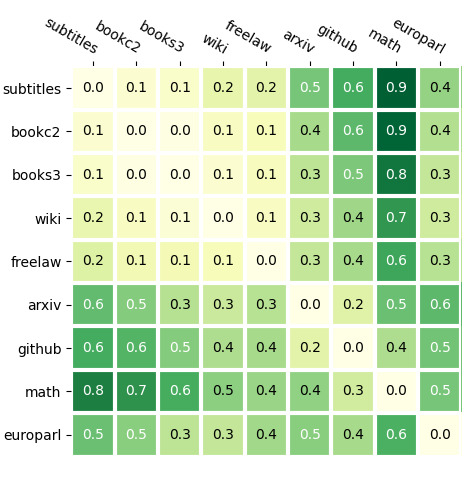
(a) Mutual Information Loss

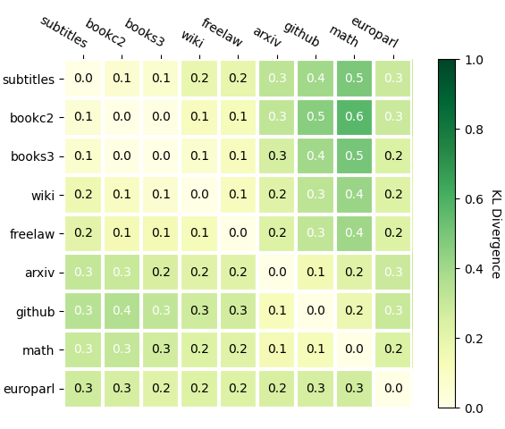
(b) ST-MoE loss

Figure 2: KL-divergence between different domains of Pile test set. We collected expert activation frequencies for MLP experts of MoLM-4B-K2 and our ST-MoE baseline on different domains of the Pile test set. We computed the KL-divergency between domains from these expert distributions for both MoLM-4B-K2 and ST-MoE baseline. Lower KL-divergence means similar expert distribution for two domains.

Analysis of expert distribution

We further collected expert distribution for MLP experts of MoLM-4B-K2 and our ST-MoE baseline on different domains of the Pile test set. Figure 2 shows the KL-divergency of expert distribution between domains. We noticed two interesting phenomenons: 1) Similar domains have smaller KL divergence; 2) ST-MoE has smaller KL-divergence values compared to MoLM model, which suggests more confounding of experts between domains. This result suggests that MI loss encourages a stronger correlation between the input category and experts, thus better at incentive modularity than the ST-MoE load balancing loss.

5.2 Learning New Knowledge with New Modules

Experiment Settings

In this section, we study two experiment settings: continual joint pre-training (Section 5.2) and continual lifelong pre-training (Section 5.2). The difference lies in the presence or absence of English texts. We continually pre-train ModuleFormer and GPT-Neo for both settings on languages in CC-100 Corpus (Wenzek et al., 2020; Conneau et al., 2020). To evaluate quality, we employ the mLAMA benchmark (Kassner et al., 2021) with the zero-shot setting used in XGLM (Lin et al., 2022) and mGPT (Shliazhko et al., 2022). More details can be found in Appendix C.

Table 5: Continual Joint Pre-Training Result (accuracy$\uparrow$).

	Model	Trainable	Continual Training (de)		Continual Training (vi)
		Params	en	de	en	vi
Freeze All	GPT-Neo-2.7B	0	78.6	64.5	78.6	58.9
	MoLM-4B-K4	0	80.9	67.8	80.9	58.4
Full Finetune	GPT-Neo-2.7B	2.7B	75.1(-3.5)	71.0(+6.5)	75.1(-3.5)	66.0(+7.1)
	MoLM-4B-K4	4B	80.1(-0.8)	71.5(+3.7)	80.1(-0.8)	67.9(+9.5)
LoRA	GPT-Neo-2.7B	159M	75.8(-2.8)	66.3(+1.8)	75.3(-3.3)	60.4(+1.5)
Insert New Experts	MoLM-4B-K4	164M	79.5(-1.4)	69.9(+2.1)	79.5(-1.4)	64.5(+6.1)

Table 6: Continual Lifelong Pre-Training Result (accuracy$\uparrow$).

	Model	Trainable	Regularization	Continual Training (vi)
		Params		en	vi
Freeze All	GPT-Neo-2.7B	0	N/A	78.6	58.9
	MoLM-4B-K4	0	N/A	80.9	58.4
LoRA	GPT-Neo-2.7B	133M	N/A	70.3(-8.3)	59.8(+1.4)
	GPT-Neo-2.7B	24M	N/A	69.3(-9.3)	57.5(-1.4)
	GPT-Neo-2.7B	133M	0.25 Weight Decay	69.9(-8.7)	57.8(-0.6)
Insert New Experts	MoLM-4B-K4	151M	$0.00$ Rout Reg	74.5(-6.4)	68.0(+9.6)
	MoLM-4B-K4	151M	$0.25$ Rout Reg	76.0(-4.9)	64.8(+6.4)
	MoLM-4B-K4	151M	$0.50$ Rout Reg	76.3(-4.6)	64.5(+6.1)
	MoLM-4B-K4	151M	$1.00$ Rout Reg	78.7(-2.2)	63.0(+4.6)

Continual Joint Pre-Training

In this part, we perform continual pre-training on models with joint training. Specifically, we mixed English and a new language to form a new training corpus, and kept the embedding layer trainable. Joint Training (Caruana, 1997) is a well-known method for multitask learning that demonstrates proficiency in both old and new tasks (Chen and Liu, 2018). However, it often creates negative interference between different tasks (Gupta et al., 2022).

Table 5 presents the results obtained from the continually trained models. The table reveals the following findings: 1) Consistent with previous studies (Gupta et al., 2022), we observed that sparse models experience less interference, ultimately leading to better full finetune performance; 2) In terms of efficient tuning, our proposed ModuleFormer also demonstrates consistently better results compared to the baseline. This suggests that low interference comes mainly from the sparse architecture rather than a large number of trainable parameters.

Continual Lifelong Pre-Training

For these experiments, the models are trained only on new language texts. Abraham and Robins (2005) proposed the stability-plasticity dilemma that explains a difficult challenge for models: 1) models should have high plasticity to learn a new language, 2) models must possess exceptional stability, considering it would not be exposed to any English tokens through the numerous training iterations.

Table 6 shows the results of the LoRA baseline and our method with different weights of the routing regularization loss. Our ModuleFormer exhibits a strong ability to balance and trade-off stability-plasticity with the help of the routing regularization loss. When we restrict the usage of new experts by increasing the loss weight, the model gains stability and loss in plasticity. In contrast, fine-tuning GPT-Neo with LoRA falls behind on both stability and plasticity. For comparison, LoRA is worse on both plasticity and stability. Reducing the number of trainable parameters (lower-rank) and applying weight decay to LoRA weights won’t improve neither plasticity or stability.

5.3 Finetuning and Pruning Modules

Previous results show that MoLM has specialized experts for different domains. In this section, we demonstrate that MoLM can be pruned to create a domain-specialized model by pruning the unused experts. The resulting model is significantly smaller in size but maintains similar performance.

We propose two pruning strategies: 1) pruning by activation frequency first and then fine-tuning on the target domain; 2) fine-tuning on the target domain with load concentration loss and then pruning by activation frequency. The first strategy achieves better overall performance for different pruning ratios. However, the second strategy only requires one fine-tuning process to enable different pruning ratios, which enables dynamically adjusting model size during inference.

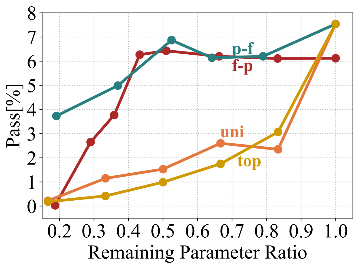
(a) Pass@1

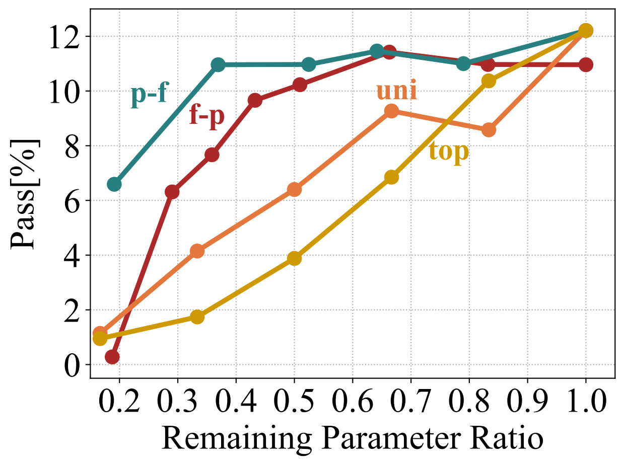
(b) Pass@10

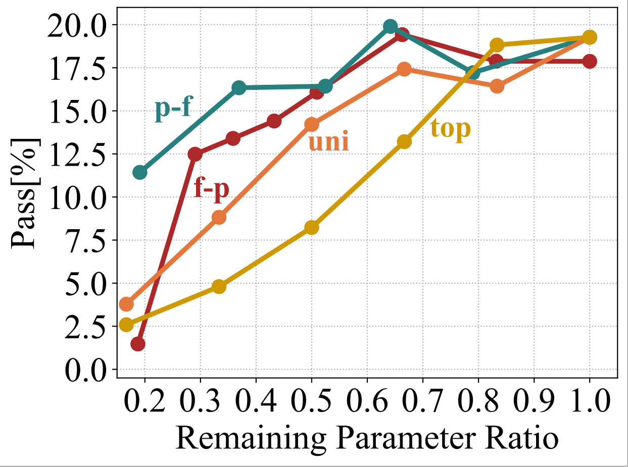
(c) Pass@100

Figure 3: Performance after Pruning on the HumanEval Dataset. The f-p is MoLM-4B-K2 finetuned with load concentration loss and then pruned with expert frequency. The p-f is MoLM-4B-K2 that is pruned with expert frequency first and then finetuned on python corpus. The uni and top is MoLM-4B-K2 that is pruned by uniformly dropping layers or dropping the top layers.

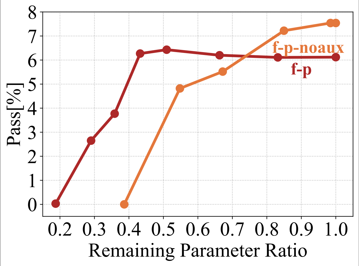
(a) Pass@1

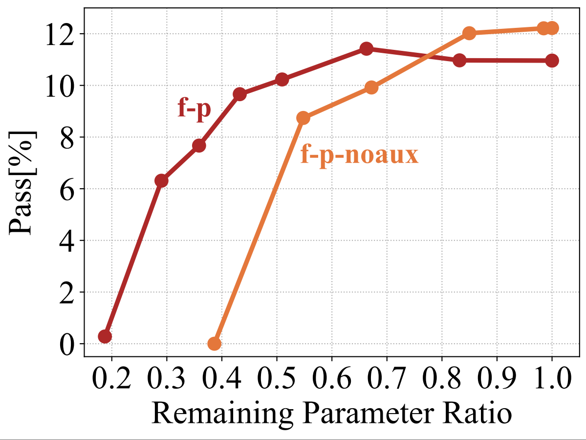
(b) Pass@10

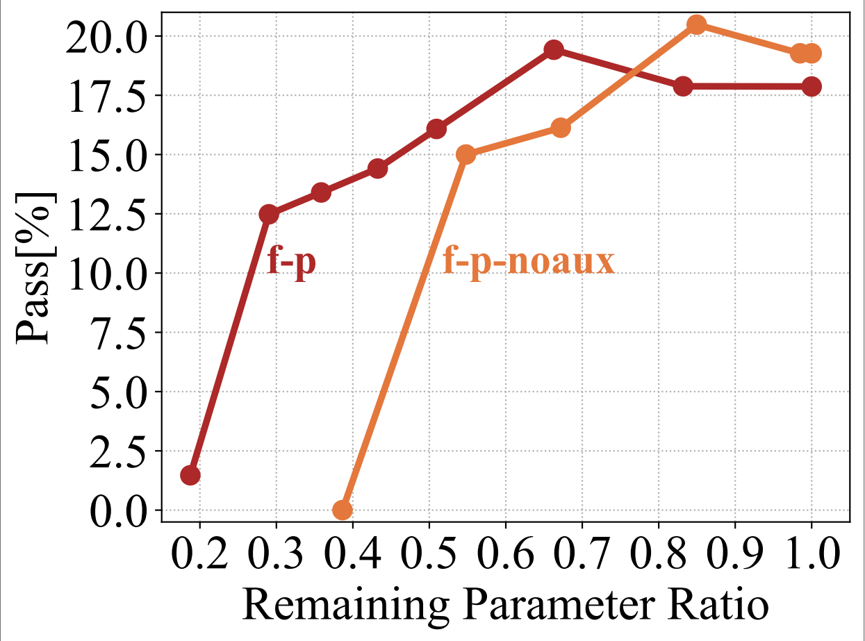
(c) Pass@100

Figure 4: Ablation study for the load concentration loss. The f-p_noaux is MoLM-4B-K2 finetuned without load concentration loss and then pruned with expert frequency.

Finetuning

We finetune our pretrained model on a 15B token subset of the GitHub-code-clean dataset (Tunstall et al., 2022) containing only Python code. When we finetune the original model, we add the load concentration loss introduced in Section 4.2 with a weight of $0.001$. More details for finetuning can be found in Appendix D.

Pruning

We count the activation frequency of each expert on the evaluation set to get the correlation between experts and the targeted domain. We then normalize the frequency by dividing the maximum frequency inside each layer. After that, we set a threshold $\tau$ and pruned all the modules whose normalized frequency fell below the threshold.

Baselines

We compare our pruning method with standard layer-wise pruning methods (Sajjad et al., 2023). Specifically, we compared dropping top and uniformly dropping layers with different ratios.

Evaluation

We test our Pruned MoLM-4B-K2 Model on the HumanEval dataset Chen et al. (2021). Figure 3 illustrates the correlation between pass@k metrics and the remaining parameter ratios. We observe that pruning unnecessary modules does not significantly impact the results. We can prune 40% to 50% of the parameters without sacrificing performance, while the layer-wise pruning method results in a visible performance drop and consistently under-performance module pruning; 2) Our fine-tuning then pruning schema achieves similar performance as pruning then fine-tuning method, while only needs to fine-tune the model once; 3) After fine-tuning with load concentration loss, there are significant disparities in the distribution of modules, with around half of the modules’ activation frequency being less than 0.3% of the most frequently used experts.

Figure 4 shows the ablation of load concentration loss. Without the load concentration loss, the model performs better for a high remaining parameter ratio (>75%). However, the loss of load concentration enables a better performance from 30% to 75% remaining parameter ratio. These results show that our load concentration loss could enable a more flexible deployment strategy for devices with different capacities. More finetuning results can be found in Appendix D.

6 Conclusion and Limitations

Conclusion

In this paper, we propose a new modular architecture, ModuleFormer, and its associated methods for module manipulation. ModuleFormer includes several new components: a new stick-breaking attention heads, a new mutual information load balancing loss for pretraining, and a new load concentration loss for finetuning. Based on ModuleFormer, we pretrained a new language model, MoLM. Our experiment result shows the promising abilities of MoLM: 1) It achieves the same performance as dense LLMs with lower latency (50%) and a smaller memory footprint; thus, it improves the throughput to more than 2 times; 2) It is less susceptible to catastrophic forgetting after finetuning the entire model on a new domain, and it could also be easily extended with new modules to learn a new language; 3) It can be finetuned on a downstream task to specialize a subset of modules on the task and the unused modules can be pruned without sacrificing the performance.

Limitations

Although it is more efficient, the MoLM uses more parameters to achieve performance comparable to dense models. We believe this is due to the optimization difficulty caused by the discrete gating decision in SMoE. How optimal gating can be learned remains an open question.

Appendix A Stick-breaking Self-attention

To restate Equation (4),

$$p_{i,t}=\beta_{i,t}\prod_{i<j\leq t}\left(1-\beta_{j,t}\right)$$ (11)

We can view $p_{t}$ as a distribution over $i$. The cumulative mass function for attending from timestep $t$ to $k$ timesteps in the past is then,

$$\sum_{t-k\leq i\leq t}\left[\beta_{i,t}\prod_{i<j\leq t}\left(1-\beta_{j,t}\right)\right]$$ (12)

$$=\beta_{t,t}+\beta_{t-1,t}(1-\beta_{t,t})+\cdots+\beta_{t-k,t}\prod_{t-k<j\leq t}\left(1-\beta_{j,t}\right)$$ (13)

If we let $$\alpha_{i,j}=1-\beta_{i,j} i,j$$ for all

$$=(1-\alpha_{t,t})+(1-\alpha_{t-1,t})~{}\alpha_{t,t}+\cdots+(1-\alpha_{t-k,t})\prod_{t-k<j\leq t}\alpha_{j,t}$$ (14)

and by telescoping cancellation,

$$=1-\prod_{t-k\leq j\leq t}\alpha_{j,t}$$ (15)

$$=1-\prod_{t-k\leq j\leq t}(1-\beta_{j,t})$$ (16)

Since $\beta_{j,t}\in(0,1)$, $(1-\beta_{j,t})\in(0,1)$. Therefore, as $k$ increases (longer context window), Equation (12) approaches 1.

Appendix B Pretraining Hyperparameters

Table 7: Pretraining Hyperparameters

Optimizer	AdamW
Maximum Learning Rate	3e-4
Minimum Learning Rate	3e-5
Weight Decay	0.01
Gradient Clipping	1.0
Training Tokens	360B
Number of Epochs	1
Warmup Tokens	3B
Batch Tokens	3M
Input Sequence Length	512

Appendix C Continual Learning Experiment Details

C.1 Dataset Details

CC-100 [Wenzek et al., 2020, Conneau et al., 2020] is a multilingual corpus that collects texts from CommonCrawl in 100 languages. For joint training setting, we incorporate newly learned languages along with English texts at a ratio of 4:1. Additionally, in order to demonstrate our efficiency, we limit our training to only 6 billion tokens.

C.2 Benchmark Details

The benchmark, mLAMA [Kassner et al., 2021] offers fill-in-the-blank questions that require comprehensive knowledge, such as birthplace, capital city, and so on. As previous works, we randomly replaced the blank with two incorrect answers among all candidates in mLAMA to test whether the correct sentence is the most unperplexed one.

C.3 Baselines Details

GPT-Neo [Gao et al., 2020] is a GPT-2 like large language dense model, pretrained on the pile [Gao et al., 2020], the same corpus we used.

LoRA [Hu et al., 2021] is a state-of-the-art method for parameter-efficient large language models adaptation. In practice, the rank in the LoRA method is frequently referred to using small numbers, such as $16$ or $32$. In our experiment, we employ LoRA in both a small and medium rank setting to regulate the number of trainable parameters.

C.4 Continual Training Hyperparameters

Table 8: Continual Training Hyperparameters

Training Tokens	6B
Number of Epochs	1
Warmup Tokens	3B
Batch Tokens	327680
Learning Rate	3e-4
Learning Rate Scheduler	Constant

C.5 Continual Training Ablation

Table 9 presents the findings from the continual training ablation study. The results indicate that: 1) With proper routing regularization, a partially trainable router strictly outperforms a fully trainable one. 2) Generally, joint training tends to yield superior overall performance compared to lifelong training, and exceptions only occur in new language abilities with low regularization.

Table 9: Comparison of different continual learning methods

	Trainable	Router	Continual Training (vi)
	Params	Tuning	en	vi
Continual Joint Pre-Training	164M	Full + load balancing	79.5(-1.4)	64.5(+6.1)
	151M	Partial	79.5(-1.4)	65.1(+6.7)
	151M	Partial + $0.25$ Rout Reg	80.1(-0.8)	65.0(+6.6)
	151M	Partial + $0.50$ Rout Reg	80.3(-0.6)	65.0(+6.6)
	151M	Partial + $1.00$ Rout Reg	80.5(-0.4)	64.1(+5.7)
Continual Lifelong Pre-Training	164M	Full + load balancing	73.8(-7.1)	66.0(+7.6)
	151M	Partial	74.5(-6.4)	68.0(+9.6)
	151M	Partial + $0.25$ Rout Reg	76.0(-4.9)	64.8(+6.4)
	151M	Partial + $0.50$ Rout Reg	76.3(-4.6)	64.5(+6.1)
	151M	Partial + $1.00$ Rout Reg	78.7(-2.2)	63.0(+4.6)

Appendix D Finetuning and Pruning

D.1 Finetuning Hyperparameters

Table 10: Finetuning Hyperparameters

Finetuning tokens	15B
Number of Epochs	2
Warmup Tokens	3B
Batch tokens	1.5M
Learning Rate	5e-5
Learning Rate Scheduler	Constant

D.2 Pruning Ablation

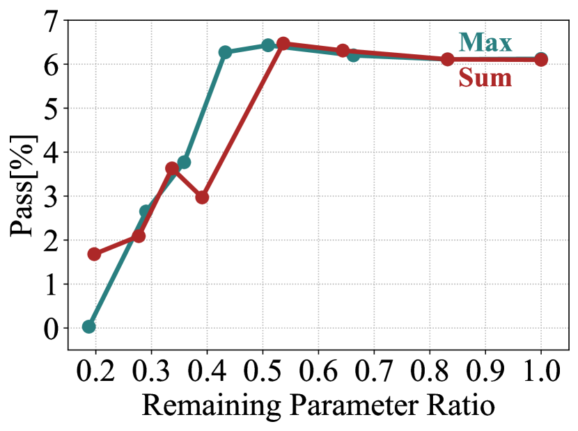
(a) ratios-pass@1

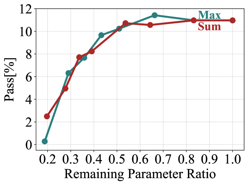
(b) ratios-pass@10

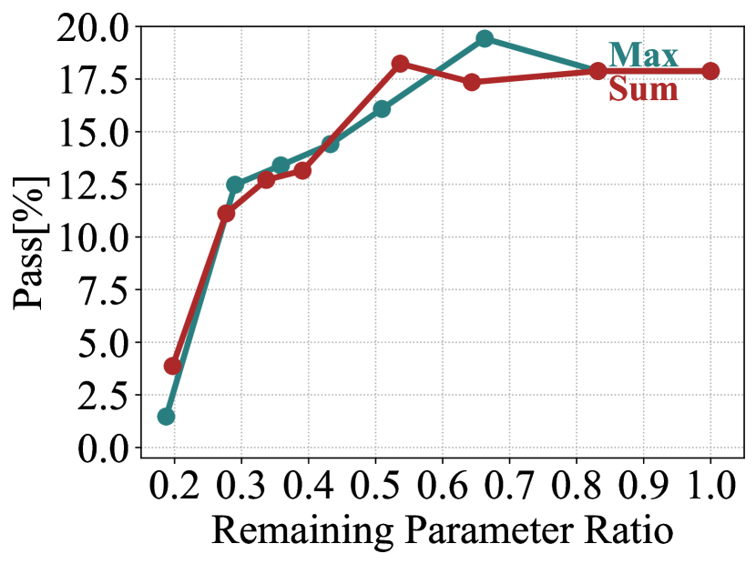
(c) ratios-pass@100

Figure 5: Performances of different pruning methods. Max means that the expert frequency is normalized with the maximum frequency inside each layer. Sum means that the expert frequency is normalized with the total activation frequency of each layer.

Fig. 5 compares the different pruning methods. While both methods leverage the activation frequency of each expert to prune the model, how to normalize the frequency still makes some differences. Max means that the expert frequency is normalized with the maximum frequency inside each layer. Sum means that the expert frequency is normalized with the total activation frequency of each layer. We found that the two methods achieve comparable results for pass@10 and pass@100, but the Max achieves better results for pass@1. Thus we choose the Max method as the major results reported in the paper.

References

- Abraham and Robins [2005] Wickliffe C Abraham and Anthony Robins. Memory retention–the synaptic stability versus plasticity dilemma. Trends in neurosciences, 28(2):73–78, 2005.
- Aghajanyan et al. [2021] Armen Aghajanyan, Anchit Gupta, Akshat Shrivastava, Xilun Chen, Luke Zettlemoyer, and Sonal Gupta. Muppet: Massive multi-task representations with pre-finetuning. arXiv preprint arXiv:2101.11038, 2021.
- Alsentzer et al. [2019] Emily Alsentzer, John Murphy, William Boag, Wei-Hung Weng, Di Jindi, Tristan Naumann, and Matthew McDermott. Publicly available clinical BERT embeddings. In Proceedings of the 2nd Clinical Natural Language Processing Workshop, pages 72–78, Minneapolis, Minnesota, USA, June 2019. Association for Computational Linguistics. doi: 10.18653/v1/W19-1909. URL https://aclanthology.org/W19-1909.
- Andreas et al. [2016] Jacob Andreas, Marcus Rohrbach, Trevor Darrell, and Dan Klein. Neural module networks. In Proceedings of the IEEE conference on computer vision and pattern recognition, pages 39–48, 2016.
- Banino et al. [2021] Andrea Banino, Jan Balaguer, and Charles Blundell. Pondernet: Learning to ponder. arXiv preprint arXiv:2107.05407, 2021.
- Beaulieu et al. [2020] Shawn Beaulieu, Lapo Frati, Thomas Miconi, Joel Lehman, Kenneth O Stanley, Jeff Clune, and Nick Cheney. Learning to continually learn. arXiv preprint arXiv:2002.09571, 2020.
- Beltagy et al. [2019] Iz Beltagy, Kyle Lo, and Arman Cohan. Scibert: A pretrained language model for scientific text. arXiv preprint arXiv:1903.10676, 2019.
- Biderman et al. [2023] Stella Biderman, Hailey Schoelkopf, Quentin Anthony, Herbie Bradley, Kyle O’Brien, Eric Hallahan, Mohammad Aflah Khan, Shivanshu Purohit, USVSN Sai Prashanth, Edward Raff, et al. Pythia: A suite for analyzing large language models across training and scaling. arXiv preprint arXiv:2304.01373, 2023.
- Brown et al. [2020] Tom Brown, Benjamin Mann, Nick Ryder, Melanie Subbiah, Jared D Kaplan, Prafulla Dhariwal, Arvind Neelakantan, Pranav Shyam, Girish Sastry, Amanda Askell, et al. Language models are few-shot learners. Advances in neural information processing systems, 33:1877–1901, 2020.
- Caruana [1997] Rich Caruana. Multitask learning. Machine learning, 28:41–75, 1997.
- Chakrabarty et al. [2019] Tuhin Chakrabarty, Christopher Hidey, and Kathy McKeown. IMHO fine-tuning improves claim detection. In Proceedings of the 2019 Conference of the North American Chapter of the Association for Computational Linguistics: Human Language Technologies, Volume 1 (Long and Short Papers), pages 558–563, Minneapolis, Minnesota, June 2019. Association for Computational Linguistics. doi: 10.18653/v1/N19-1054. URL https://aclanthology.org/N19-1054.
- Chen et al. [2021] Mark Chen, Jerry Tworek, Heewoo Jun, Qiming Yuan, Henrique Ponde de Oliveira Pinto, Jared Kaplan, Harri Edwards, Yuri Burda, Nicholas Joseph, Greg Brockman, et al. Evaluating large language models trained on code. arXiv preprint arXiv:2107.03374, 2021.
- Chen and Liu [2018] Zhiyuan Chen and Bing Liu. Continual learning and catastrophic forgetting. In Lifelong Machine Learning, pages 55–75. Springer, 2018.
- Chen et al. [2022] Zitian Chen, Yikang Shen, Mingyu Ding, Zhenfang Chen, Hengshuang Zhao, Erik Learned-Miller, and Chuang Gan. Mod-squad: Designing mixture of experts as modular multi-task learners. arXiv preprint arXiv:2212.08066, 2022.
- Chowdhery et al. [2022] Aakanksha Chowdhery, Sharan Narang, Jacob Devlin, Maarten Bosma, Gaurav Mishra, Adam Roberts, Paul Barham, Hyung Won Chung, Charles Sutton, Sebastian Gehrmann, et al. Palm: Scaling language modeling with pathways. arXiv preprint arXiv:2204.02311, 2022.
- Conneau et al. [2020] Alexis Conneau, Kartikay Khandelwal, Naman Goyal, Vishrav Chaudhary, Guillaume Wenzek, Francisco Guzmán, Edouard Grave, Myle Ott, Luke Zettlemoyer, and Veselin Stoyanov. Unsupervised cross-lingual representation learning at scale. In Proceedings of the 58th Annual Meeting of the Association for Computational Linguistics, pages 8440–8451, Online, July 2020. Association for Computational Linguistics. doi: 10.18653/v1/2020.acl-main.747. URL https://aclanthology.org/2020.acl-main.747.
- Csordás et al. [2021] Róbert Csordás, Kazuki Irie, and Jürgen Schmidhuber. The neural data router: Adaptive control flow in transformers improves systematic generalization. arXiv preprint arXiv:2110.07732, 2021.
- Dai et al. [2019] Zihang Dai, Zhilin Yang, Yiming Yang, Jaime Carbonell, Quoc V Le, and Ruslan Salakhutdinov. Transformer-xl: Attentive language models beyond a fixed-length context. arXiv preprint arXiv:1901.02860, 2019.
- Dehghani et al. [2018] Mostafa Dehghani, Stephan Gouws, Oriol Vinyals, Jakob Uszkoreit, and Łukasz Kaiser. Universal transformers. arXiv preprint arXiv:1807.03819, 2018.
- Devlin et al. [2018] Jacob Devlin, Ming-Wei Chang, Kenton Lee, and Kristina Toutanova. Bert: Pre-training of deep bidirectional transformers for language understanding. arXiv preprint arXiv:1810.04805, 2018.
- Fedus et al. [2021] William Fedus, Barret Zoph, and Noam Shazeer. Switch transformers: Scaling to trillion parameter models with simple and efficient sparsity, 2021.
- Frankle and Carbin [2018] Jonathan Frankle and Michael Carbin. The lottery ticket hypothesis: Finding sparse, trainable neural networks. arXiv preprint arXiv:1803.03635, 2018.
- Frantar and Alistarh [2023] Elias Frantar and Dan Alistarh. Sparsegpt: Massive language models can be accurately pruned in one-shot, 2023.
- Gao et al. [2020] Leo Gao, Stella Biderman, Sid Black, Laurence Golding, Travis Hoppe, Charles Foster, Jason Phang, Horace He, Anish Thite, Noa Nabeshima, et al. The pile: An 800gb dataset of diverse text for language modeling. arXiv preprint arXiv:2101.00027, 2020.
- Graves [2016] Alex Graves. Adaptive computation time for recurrent neural networks. arXiv preprint arXiv:1603.08983, 2016.
- Gupta et al. [2022] Shashank Gupta, Subhabrata Mukherjee, Krishan Subudhi, Eduardo Gonzalez, Damien Jose, Ahmed H Awadallah, and Jianfeng Gao. Sparsely activated mixture-of-experts are robust multi-task learners. arXiv preprint arXiv:2204.07689, 2022.
- Gururangan et al. [2021] Suchin Gururangan, Mike Lewis, Ari Holtzman, Noah A Smith, and Luke Zettlemoyer. Demix layers: Disentangling domains for modular language modeling. arXiv preprint arXiv:2108.05036, 2021.
- He et al. [2017] Yihui He, Xiangyu Zhang, and Jian Sun. Channel pruning for accelerating very deep neural networks. In Proceedings of the IEEE international conference on computer vision, pages 1389–1397, 2017.
- Houlsby et al. [2019] Neil Houlsby, Andrei Giurgiu, Stanislaw Jastrzebski, Bruna Morrone, Quentin De Laroussilhe, Andrea Gesmundo, Mona Attariyan, and Sylvain Gelly. Parameter-efficient transfer learning for nlp. In International Conference on Machine Learning, pages 2790–2799. PMLR, 2019.
- Hu et al. [2021] Edward J Hu, Yelong Shen, Phillip Wallis, Zeyuan Allen-Zhu, Yuanzhi Li, Shean Wang, Lu Wang, and Weizhu Chen. Lora: Low-rank adaptation of large language models. arXiv preprint arXiv:2106.09685, 2021.
- Kassner et al. [2021] Nora Kassner, Philipp Dufter, and Hinrich Schütze. Multilingual lama: Investigating knowledge in multilingual pretrained language models. arXiv preprint arXiv:2102.00894, 2021.
- Kirkpatrick et al. [2017] James Kirkpatrick, Razvan Pascanu, Neil Rabinowitz, Joel Veness, Guillaume Desjardins, Andrei A Rusu, Kieran Milan, John Quan, Tiago Ramalho, Agnieszka Grabska-Barwinska, et al. Overcoming catastrophic forgetting in neural networks. Proceedings of the national academy of sciences, 114(13):3521–3526, 2017.
- Lazaridou et al. [2022] Angeliki Lazaridou, Elena Gribovskaya, Wojciech Stokowiec, and Nikolai Grigorev. Internet-augmented language models through few-shot prompting for open-domain question answering. arXiv preprint arXiv:2203.05115, 2022.
- LeCun et al. [1989] Yann LeCun, John Denker, and Sara Solla. Optimal brain damage. Advances in neural information processing systems, 2, 1989.
- Lee et al. [2020] Jinhyuk Lee, Wonjin Yoon, Sungdong Kim, Donghyeon Kim, Sunkyu Kim, Chan Ho So, and Jaewoo Kang. Biobert: a pre-trained biomedical language representation model for biomedical text mining. Bioinformatics, 36(4):1234–1240, 2020.
- Lepikhin et al. [2020] Dmitry Lepikhin, HyoukJoong Lee, Yuanzhong Xu, Dehao Chen, Orhan Firat, Yanping Huang, Maxim Krikun, Noam Shazeer, and Zhifeng Chen. Gshard: Scaling giant models with conditional computation and automatic sharding. arXiv preprint arXiv:2006.16668, 2020.
- Lesort et al. [2019] Timothée Lesort, Andrei Stoian, and David Filliat. Regularization shortcomings for continual learning. arXiv preprint arXiv:1912.03049, 2019.
- Li et al. [2016] Hao Li, Asim Kadav, Igor Durdanovic, Hanan Samet, and Hans Peter Graf. Pruning filters for efficient convnets. arXiv preprint arXiv:1608.08710, 2016.
- Li and Hoiem [2017] Zhizhong Li and Derek Hoiem. Learning without forgetting. IEEE transactions on pattern analysis and machine intelligence, 40(12):2935–2947, 2017.
- Lin et al. [2022] Xi Victoria Lin, Todor Mihaylov, Mikel Artetxe, Tianlu Wang, Shuohui Chen, Daniel Simig, Myle Ott, Naman Goyal, Shruti Bhosale, Jingfei Du, et al. Few-shot learning with multilingual generative language models. In Proceedings of the 2022 Conference on Empirical Methods in Natural Language Processing, pages 9019–9052, 2022.
- Lin et al. [2020] Zhaojiang Lin, Andrea Madotto, and Pascale Fung. Exploring versatile generative language model via parameter-efficient transfer learning. arXiv preprint arXiv:2004.03829, 2020.
- Liu et al. [2018] Zhuang Liu, Mingjie Sun, Tinghui Zhou, Gao Huang, and Trevor Darrell. Rethinking the value of network pruning. arXiv preprint arXiv:1810.05270, 2018.
- Loshchilov and Hutter [2017] Ilya Loshchilov and Frank Hutter. Decoupled weight decay regularization. arXiv preprint arXiv:1711.05101, 2017.
- McCloskey and Cohen [1989] Michael McCloskey and Neal J Cohen. Catastrophic interference in connectionist networks: The sequential learning problem. In Psychology of learning and motivation, volume 24, pages 109–165. Elsevier, 1989.
- Munkhdalai and Yu [2017] Tsendsuren Munkhdalai and Hong Yu. Meta networks. In International conference on machine learning, pages 2554–2563. PMLR, 2017.
- Nijkamp et al. [2022] Erik Nijkamp, Bo Pang, Hiroaki Hayashi, Lifu Tu, Huan Wang, Yingbo Zhou, Silvio Savarese, and Caiming Xiong. Codegen: An open large language model for code with multi-turn program synthesis. arXiv preprint arXiv:2203.13474, 2022.
- Press et al. [2021] Ofir Press, Noah A Smith, and Mike Lewis. Train short, test long: Attention with linear biases enables input length extrapolation. arXiv preprint arXiv:2108.12409, 2021.
- Radford et al. [2019] Alec Radford, Jeffrey Wu, Rewon Child, David Luan, Dario Amodei, Ilya Sutskever, et al. Language models are unsupervised multitask learners. OpenAI blog, 1(8):9, 2019.
- Rebuffi et al. [2017] Sylvestre-Alvise Rebuffi, Hakan Bilen, and Andrea Vedaldi. Learning multiple visual domains with residual adapters. Advances in neural information processing systems, 30, 2017.
- Sajjad et al. [2023] Hassan Sajjad, Fahim Dalvi, Nadir Durrani, and Preslav Nakov. On the effect of dropping layers of pre-trained transformer models. Computer Speech & Language, 77:101429, 2023.
- Samarakoon and Sim [2016] Lahiru Samarakoon and Khe Chai Sim. Low-rank bases for factorized hidden layer adaptation of dnn acoustic models. In 2016 IEEE Spoken Language Technology Workshop (SLT), pages 652–658. IEEE, 2016.
- Shazeer et al. [2017] Noam Shazeer, Azalia Mirhoseini, Krzysztof Maziarz, Andy Davis, Quoc Le, Geoffrey Hinton, and Jeff Dean. Outrageously large neural networks: The sparsely-gated mixture-of-experts layer. arXiv preprint arXiv:1701.06538, 2017.
- Shliazhko et al. [2022] Oleh Shliazhko, Alena Fenogenova, Maria Tikhonova, Vladislav Mikhailov, Anastasia Kozlova, and Tatiana Shavrina. mgpt: Few-shot learners go multilingual. arXiv preprint arXiv:2204.07580, 2022.
- Su et al. [2021] Jianlin Su, Yu Lu, Shengfeng Pan, Ahmed Murtadha, Bo Wen, and Yunfeng Liu. Roformer: Enhanced transformer with rotary position embedding. arXiv preprint arXiv:2104.09864, 2021.
- Sun et al. [2022] Yutao Sun, Li Dong, Barun Patra, Shuming Ma, Shaohan Huang, Alon Benhaim, Vishrav Chaudhary, Xia Song, and Furu Wei. A length-extrapolatable transformer. arXiv preprint arXiv:2212.10554, 2022.
- Tan and Sim [2016] Shawn Tan and Khe Chai Sim. Towards implicit complexity control using variable-depth deep neural networks for automatic speech recognition. In 2016 IEEE International Conference on Acoustics, Speech and Signal Processing (ICASSP), pages 5965–5969. IEEE, 2016.
- Touvron et al. [2023] Hugo Touvron, Thibaut Lavril, Gautier Izacard, Xavier Martinet, Marie-Anne Lachaux, Timothée Lacroix, Baptiste Rozière, Naman Goyal, Eric Hambro, Faisal Azhar, et al. Llama: Open and efficient foundation language models. arXiv preprint arXiv:2302.13971, 2023.
- Tunstall et al. [2022] Lewis Tunstall, Leandro Von Werra, and Thomas Wolf. Natural language processing with transformers. " O’Reilly Media, Inc.", 2022.
- Vaswani et al. [2017] Ashish Vaswani, Noam Shazeer, Niki Parmar, Jakob Uszkoreit, Llion Jones, Aidan N Gomez, Łukasz Kaiser, and Illia Polosukhin. Attention is all you need. Advances in neural information processing systems, 30, 2017.
- Wang et al. [2020] Yulong Wang, Xiaolu Zhang, Lingxi Xie, Jun Zhou, Hang Su, Bo Zhang, and Xiaolin Hu. Pruning from scratch. In Proceedings of the AAAI Conference on Artificial Intelligence, volume 34, pages 12273–12280, 2020.
- Wenzek et al. [2020] Guillaume Wenzek, Marie-Anne Lachaux, Alexis Conneau, Vishrav Chaudhary, Francisco Guzmán, Armand Joulin, and Edouard Grave. CCNet: Extracting high quality monolingual datasets from web crawl data. In Proceedings of the Twelfth Language Resources and Evaluation Conference, pages 4003–4012, Marseille, France, May 2020. European Language Resources Association. ISBN 979-10-95546-34-4. URL https://aclanthology.org/2020.lrec-1.494.
- Zhang et al. [2022] Xiaofeng Zhang, Yikang Shen, Zeyu Huang, Jie Zhou, Wenge Rong, and Zhang Xiong. Mixture of attention heads: Selecting attention heads per token. arXiv e-prints, pages arXiv–2210, 2022.
- Zoph et al. [2022] Barret Zoph, Irwan Bello, Sameer Kumar, Nan Du, Yanping Huang, Jeff Dean, Noam Shazeer, and William Fedus. St-moe: Designing stable and transferable sparse expert models. arXiv preprint arXiv:2202.08906, 2022.