Fair Multi-Agent Bandits

Abstract

In this paper, we study the problem of fair multi-agent multi-arm bandit learning when agents do not communicate with each other, except collision information, provided to agents accessing the same arm simultaneously. We provide an algorithm with regret $O\left(N^{3}\log\frac{B}{\Delta}f(\log T)\log T\right)$ (assuming bounded rewards, with unknown bound), where $f(t)$ is any function diverging to infinity with $t$. This significantly improves previous results which had the same upper bound on the regret of order $O(f(\log T)\log T)$ but an exponential dependence on the number of agents. The result is attained by using a distributed auction algorithm to learn the sample-optimal matching and a novel order-statistics-based regret analysis. Simulation results present the dependence of the regret on $\log T$.

1 Introduction

Any large system providing service to multiple agents requires resource allocation algorithms, to efficiently serve the demand of the agents. Examples include, e.g., cloud computing, management of cellular and wireless networks as well as transportation networks. The classical approach for achieving good allocations is through centralized management, where the managing entity dictates the resources allocated to each agent. With the scaling up of networks and systems, the complexity of collecting the required data required by a central management entity increases significantly, scaling like the product of the number of resources and the number of agents. The situation is further aggravated when the agents do not know their utilities of using the various resources. Therefore, distributed protocols where the cooperating agents make local decisions on which resources to use become essential. These distributed protocols must be designed to allow agents to sense and learn their utilities independently of the other agents.

The multi-agent multi-armed bandit setup is a good paradigm for distributedly allocating resources under uncertainty [1]. This emerging paradigm for multi-agent resource allocation has been recently the subject of extensive research efforts, see, e.g. [2, 3], [4], [5], [6], [7], [8], [9], [10], [11], [12], [13], [14], [15], [16]. Early works concentrated on the special case where each arm has the same reward distribution irrespective of the agent selecting it and optimized the sum of rewards [17], [18], [19], [20]. However, in many applications, the reward each arm provides to different agents might be different, e.g. in the context of cloud computing certain users or applications might benefit from using machines with faster CPU while others will benefit more from having access to machines with faster and larger memory. Similarly, when allocating wireless channels, different receivers might experience different interference at different frequencies resulting in different achievable data rates.

In the standard model, each agent faces the classical stochastic multi-armed bandit problem [21], but the agent is impacted by the choices of all players. The assumed model is fully cooperative, where agents are allowed to set up a joint protocol in advance, but not explicitly send messages to each other during the learning phase. Although the protocol is cooperative, agents are unaware of the other agents’ actions and rewards which can result in conflicting actions.

One approach to resolve this problem is by assigning zero rewards to players who select the same arm or equivalently providing the agents with a collision indicator, similar to the NAQ message in wireless networks. Therefore, by learning which arms to pull, the agents can jointly learn an optimal allocation distributedly. The only information an agent receives is through the collisions occurring when other agents select the same arm. This collision model captures Aloha-based protocols in communication networks, computation resources on servers, consumers splitting indivisible goods, etc. An alternative to this approach which alleviates the need for message passing is by applying a distributed auction algorithm [22] together with an access protocol based on opportunistic carrier sensing [23]. This generalization has been proposed by [14] and later extended to learning how to share the same arm distributedly among multiple players when incorporating more agents than arms [24].

Initial works on the problem focused on maximizing the total sum of agent rewards, e.g., [15], [25], [26], [1], [27], [28], [10], [18], [29]. The total sum utility metric is relevant in some applications when only the overall system utility is considered. However, in distributed environments where agents have conflicting interests while they still benefit from cooperation, there is a need to motivate all agents to collaborate. For example, any division should be individually reasonable, so that each agent receives more than what it can gain by competing. In the general cooperative game-theoretical literature, fair solutions are important means to facilitate cooperation. Examples are the seminal Nash Bargaining Solution [30], proportional fair division [31], Kalai-Smorodinski solution [32] and weighted max-min fair allocations [33], [34]. These objectives have been used extensively in the broader resource allocation literature [35, 34, 36]. In contrast fairness in multi-player bandits has only recently been studied [37], [38]. Some multi-player bandit works have studied alternative objectives that can potentially exhibit some level of fairness, e.g., [39, 40]. Several recent works have studied fairness-constrained sequential learning for a single player [41, 42, 43]. The work by Bistritiz et al. [38] also considered a quality of service guarantee, when it is known that the expected level of service is achievable. Surprisingly, in this setting, regret is bounded. However, the assumption of knowing the QoS level is feasible is strong, and not always practical. These works provide regret bounds and achievable regret for the fair multi-armed bandit problem. Unfortunately, from the computational point of view, they involve a large state space Markov chain of size $K^{N}$, where $N$ is the number of players, and $K$ is the number of arms. The state space, even for $2$ arms is of size $2^{N}$ which is huge even when $N=10$.

In this paper, we consider max-min fair solutions, where the goal is to maximize the expected reward of the worst-off player, i.e., a max-min fair solution. We provide a distributed algorithm that has provably near order-optimal regret of $f(\log T)\log T$, with respect to optimal max-min value where, $f(t)$ is any slowly diverging function, and polynomial complexity ($N^{3}$) in the number of agents. This improves prior art, which provided near-optimal regret order, but also had exponential dependence on the number of agents. Moreover, the polynomial dependence makes the proposed technique attractive in large-scale problems.

Interestingly, a simple variation of our learning algorithm provides a learning algorithm achieving any Pareto dominant allocation, through the use of weighting, similarly to the results of [34].

1.1 Prior Work on fair bandit learning

As mentioned, problems of fairness date back to Nash’s work on the bargaining problem [30]. A special case of the Nash bargaining solution is the proportional fair solution, which is equivalent to Nash’s solution when the disagreement value is $0$ for all players and leads to maximizing $\sum_{n}\log U_{n}(\mbox{${\mathbf{a}}$})$ where ${\mathbf{a}}$ is the vector of the joint actions. Another family of fairness criteria is defined by the $\alpha$-fairness metric, for a vector of rewards $\mbox{${\mathbf{u}}$}\in{\mathbb{R}}^{N}$ is $\sum_{i=1}^{N}(1-\alpha)^{-1}u_{i}^{1-\alpha}$, for $\alpha\neq 1$ [44]. This notion of fairness encompasses several classical ones, where $\alpha=0$ yields the sum of rewards, and the max-min fairness criterion corresponds to the limit as $\alpha\rightarrow\infty$. For constant $\alpha$, $\alpha$-fairness can be maximized in a similar manner to [1, 27], the case of max-min fairness is fundamentally different.

When analyzing max-min fair learning regret it is simple to show an $\Omega(\log T)$ lower bound using a reduction to the single player Lai-Robbins lower bound by adding fictitious players with high rewards (See [38], proposition 1), so the main problem is to find tight upper bounds on the problem.

Learning to play a max-min fair allocation without explicit communication between the players poses several challenges that do not arise in the case of maximizing the sum-rewards (or in the case of $\alpha$-fairness). The sum-rewards optimal allocation is unique for “almost all” scenarios (by dithering the expected rewards). In contrast, there are typically multiple max-min fair allocations. This complicates the distributed learning process since players will have to agree on a specific optimal allocation to play, which is difficult to do without communication. Specifically, this rules out using similar techniques to those used in [1] to solve the sum of rewards case. The first paper to propose a solution was [37] and its extension [38]. The first result in these papers proved near logarithmic regret for the max-min problem. Interestingly, in the second paper it was also proved that when the value of the max-min is known a bounded regret can be achieved by extending the QoS formulation in [45] and [46] which found all the “good arms” (instead of minimizing the regret). However, neither [45] nor [46] can be used for the multiplayer case since they rely on i.i.d. rewards, which is no longer the case with collisions between players. In [45] it is proved that if a number $\gamma$ between the optimal expected reward and the second-best expected reward is known, then $O(1)$ regret can be achieved for the single-player multi-armed bandit problem. This was extended to the multiplayer case in [38]. As explained above, the techniques of [38] become exponentially complex as the number of agents grows, because it relies on the convergence of an absorbing Markov chain with an exponentially large (in the number of players) state space.

In contrast in this paper, we propose to use a preliminary stage of distributedly ordering the agents, a task well-known in the distributed computation literature. Following this ordering we can utilize an efficient distributed algorithm that relies on collisions to find a max-min fair matching. This replaces the possibly exponentially long (in the number of players) matching phase (as is also used in [1, 27]) by a rapidly converging algorithm. We exploit the distributed auction algorithm to obtain the optimal max-min allocation, based on the estimated rewards. The auction algorithm has been used by [10] to obtain optimal logarithmic regret when communication between agents is possible. Later in [14] a fully distributed algorithm has been proposed for learning the sum-rate optimal allocation. However, in that paper two crucial assumptions have been made: The agents could use a listen-before-talk protocol for accessing the arms (which is equivalent to replacing ALOHA by CSMA in wireless communication networks [47]) and the rewards are discrete, so a bound on the minimum distance between the optimal reward and the second best reward is known. Using the distributed auction algorithm a standard 3-phase exploration, negotiation, and exploitation structure is utilized where we can show regret of order $N^{3}\log\frac{B}{\Delta}f(\log T)\log T$, where $B$ is a bound on the support of the rewards, $\Delta$ is the minimal gap and $f(t)$ is any diverging function, e.g., $f(t)=\log t$ would result in $O\left(\log T\log\log T\right)$ regret.

1.2 Contributions and limitations

In this paper, we utilize the auction algorithm to solve a distributed matching problem. By performing pre-processing to order the agents, we prevent random collisions, so collisions can be used for signaling or for implementing a double push step in the distributed auction. We then combine a distributed auction algorithm using a version proposed by [22] to eliminate the need for sharing the prices during the auctions. The problem of distributed computation of a maximum cardinality matching is a fundamental problem in distributed computation. A well-known solution is the auction algorithm by Bertsekas [48]. Since the original auction algorithm requires shared memory, we use the variation of [22], where it is shown that allowing each agent to maintain its own price for each object results in a factor $N$ slowdown in convergence, but the algorithm still converges to the optimum as long as $\varepsilon<\frac{1}{N}$. Since we are interested in the specific version for finding a matching, rather than a general optimal assignment, the algorithm can be simplified as discussed in [49]. In this case, at each round, a single unallocated agent is selected and the agent picks an object and removes the agent currently assigned to the object. This is equivalent to the push-relabel algorithm with double push [50, 51]. Our pre-processing ordering step makes the selection of an agent at each step simple to implement, since each agent infers its schedule distributedly, without knowing the order of the other agents. This allows us to significantly simplify the analysis and rely on the results of [22] and [49] to obtain convergence time of $O\left(N^{3}\right)$ iterations for any graph.

Based on this we propose a fully distributed, polynomial scheme to compute a max-min optimal matching in $N^{3}\log\frac{B}{\Delta}$, where $B$ is the maximal support of the arm distributions and $\Delta$ is the minimal per agent gap, using a binary search. This, distributed binary search is tricky since the agents do not know any a-priori bounds on the rewards and have to distributedly infer, this bound with sufficiently high probability. In contrast to the prior art, we assume bounded rewards with unknown support. While this is weaker than the general sub-Gaussian case it is still of great practical interest since in almost all applications, physical and computational constraints allow us to obtain such a bound, moreover, the logarithmic dependence on $B$ ensures that even for extremely high values of $B$ the regret only suffers a small multiplicative loss. The analysis technique is also novel and is based on order statistics. It provides a novel approach to implementing and analyzing multi-agent learning with bounded rewards. Interestingly, most of the proof carries to the sub-Gaussian case, but we are unable to provide simple complexity bound on the matching phase similar to the $N^{3}\log\frac{B}{\Delta}$ in the sub-Gaussian case although we conjecture that this is true. Another novelty is allowing the epoch-based algorithm to have a data-dependent phase length since our distributed matching relies on estimated quantities. This simplifies the proofs and accelerates the algorithm’s convergence. We also comment that although our results are stronger than [38] the proofs of the main theorem is also simpler.

Finally, what remains open is achieving exact logarithmic regret. Similarly to [38] we only get regret order of $f(\log T)\log T$, where $f(t)$ is any slowly diverging function of $t$.

2 The max-min fair bandit problem

Assume that $N$ agents access $M$ arms with agent-dependent mean rewards $R_{n,m}$. The agents do not know the mean rewards and cannot communicate with each other. They need to learn the optimal arm assignment. Time $t$ is discrete and synchronized. Each time an agent $n$ chooses an arm $m$ she obtains a random reward $r_{n,m}$. When two agents access the same arm simultaneously, a collision occurs and the reward of the colliding agents is $0$. We define for each arm and action profile $\mbox{${\mathbf{a}}$}=[a_{1},\ldots,a_{n}]$, where $a_{n}$ is the arm selected by agent $n$, a collision indicator $\eta_{m}(\mbox{${\mathbf{a}}$})$ by:

$$\eta_{m}(\mbox{${\mathbf{a}}$})=\left\{\begin{tabular}[]{ll}$0$&\hbox{if \ } $\left|\left\{n:a_{n}=i\right\}\right|>1$.\\ $1$&\hbox{otherwise.}\end{tabular}\right.$$ (3)

The instantaneous utility of agent $n$ at time $t$ is now given by $u_{n}(t)=\eta_{a(t)}(t)r_{n,a_{n}}(t)$. The agents are cooperating in the sense that they can follow a predefined shared protocol, but they cannot exchange information regarding the rewards they collected or their preferences. Without loss of generality, we will now assume that $N=M$, since the availability of extra arms simplifies the coordination process. The max-min allocation problem can be described as finding the value $\rho^{*}$ and permutation $\pi^{*}$ which satisfy:

$$\rho^{*} =\max_{\pi\in S_{n}}\min_{n}R_{n,\pi(n)}$$ (4)

$$\pi^{*} =\arg\max_{\pi\in S_{n}}\min_{n}R_{n,\pi(n)}$$ (5)

We can now define the (pseudo)-regret of a strategy $\pi$ as:

$$R=\sum_{t=1}^{T}\left(\rho^{*}-\min_{n}\left\{\eta_{n}(\pi_{n}(t))R_{n,\pi_{n}(t)}R_{n,a_{n}}\right\}\right)$$ (6)

In this paper, we assume that the sample rewards are positive and bounded random variables but their support is unknown to the agents. For a distribution $F(r)$, we define the support $S(F)=\inf\left\{x\in\mathbb{R}:F(x)=1\right\}$. when $F$ is the distribution of the reward of agent $n$ on arm $m$ we denote the support by $S_{n,m}$. We do not assume identical support of the arm rewards: For each agent $n$ and each arm we can have different support $S_{n,m}$.

Remark 2.1 (Bounded rewards).

While theoretically, we would be interested in the general sub-Gaussian case, from a practical point of view this limiting assumption always holds for physical reasons. Hence, the bounded rewards with unknown support is a reasonable model. We will also assume that the distribution of the arm rewards is continuous with positive density on the support of the distribution. This assumption is not necessary, but it simplifies the notation and therefore the presentation. The techniques in this paper do not carry straightforwardly to the general sub-Gaussian case, leaving this case as an interesting research problem.

Remark 2.2 (Continuously distributed rewards).

Rewards with a continuous distribution are natural in many applications (e.g. signal-to-noise ratio in wireless networks). However, this assumption is only used to argue that since the probability of zero reward in a non-collision is zero, players can properly estimate their expected rewards. In the case where there is a positive probability of receiving zero reward, we can assume instead that each player can observe their no-collision indicator in addition to their reward. This alternative assumption requires no modifications to our algorithms or analyses. Observing one bit of feedback signifying whether any other player chose the same arm is significantly less than other common feedback models, such as observing the actions of other players. In wireless networks, this could mean that the ACK is not received at the transmitter over the reverse control channel and therefore the transmitter knows there was a collision on its chosen channel.

3 Learning a max-min optimal allocation

Similarly to other cooperative learning schemes which operate under limited communication, we will use phased exploration, negotiation and learning. In contrast to previous work, we would like to order the agents, by adding an agent-ordering phase at the beginning of each epoch. This makes the exploration more efficient and allows the use of collisions to determine end of phases.

The exploration phase length will depend on the collected rewards but will slowly grow. The only requirement is that the total exploration length grows faster than linear.

In the negotiation phases an optimal matching based on the current estimates of the rewards is distributedly computed. To achieve this we propose to use a novel distributed matching protocol based on the auction algorithm for bi-partite maximum cardinality matching [52], and finally, the length of the exploitation phase will grow exponentially.

Since the support of each arm is different, we will need a coordination mechanism to end the exploration and exploitation phases. A similar approach will be used to determine distributedly, that the max-min allocation using the estimated rewards of each agent is achieved.

3.1 Agent’s ordering

As a first step We would like to determine an agreed order of the agents in order to simplify the analysis of the protocol. Therefore, we assume that the arms are ordered according to some random order, known to the players. This is not a limiting assumption, since the arms are entities that can have a fixed identifier which allows the agents to select specific arms. Using this assumption, we can use the collision mechanism on the arms to order the agents randomly. Moreover, each agent only knows her own place in the order. We can replace the pre-ordering phase with random access, but this will complicate the analysis of the subsequent phases, without any significant gain. As we will show below, this step has a low constant regret of the order $O\left(N\log N\right)$.

Ordering agents is a standard task in distributed computation, which can be done e.g., using iterative leader election, or by randomly choosing arms. For completeness, we provide a brief description of the process. To obtain an ordering of the agents we use the following protocol: Slots in this phase are divided into groups of even and odd slots: $2n,2n+1$ denoted, type $0,1$ respectively. All agents are initially unassigned. Each agent has the full list of arms as available. During type $0$ slots each assigned agent accesses its selected arm. Each unassigned agent picks a random arm from the list of available arms. If there was no collision over the given arm, it means that the arm is free and the agent is assigned to this arm and keeps this arm as its selected arm. If there was a collision over the arm during a type $0$ slot, all the unassigned agents who sampled the arm, sample the arm during the following type $1$ slot. This is used to identify a collision between unassigned agents. If an unassigned agent successfully received a positive reward during a type $1$ slot, it means that it was the only unassigned agent accessing the arm. In this case, the collision during the previous slot was with an assigned agent, so the agent removes the arm from the list of available arms. If there was a collision during this slot, it means that the arm might still be available and the agent does nothing.

We note that in the worst case, the last allocated agent performs a full coupon collection over the arms, where he collided with every allocated user. On top of these collisions, there might be collisions on free arms between unallocated agents during type 0,1 slots. However, using standard analysis of random access protocols and the coupon collection problem, after every $2\beta N\log N$ slots of the allocation process, the probability of having an unassigned agent is approximately, $n^{-\beta}$. Picking $\beta=4$ the probability of having an unassigned agent is very small even for a small number of agents. Hence after $\beta N\log N$ slots, any unassigned agent samples all arms to notify that the process continues. Once an assigned agent observes a continuous block of $8N\log N+N$ slots without collisions on its phase $0$ slots the order is achieved, and the agent knows its order in the subsequent rounds. Since, the probability of failure in the coupon collection problem decays as $N^{-4}$, when the number of rounds is $O(8N\log N)$, by the Borel-Cantelli lemma, the process terminates with probability 1, yielding a bounded initial regret $R_{0}$ during this phase. The ordering phase is described in Algorithm 2 in the appendix.

Following the ordering initial phase, the algorithm is divided into epochs of varying lengths. One of the novel ideas in this paper is the use of upper confidence bound on the support of the distribution to determine the length of the phases in a way that allows to bound the regret. As described in Algorithm 1 the learning continues in epochs, each comprised of 3 phases, similarly to [27].

1:  Initialization of agent $n$:

2:  $N$ is the number of agents.

3:  $M$ is the number of arms.

4:  $\mbox{${\hat{R}}$}_{n,m}\leftarrow 0$ for all $m$.

5:  $V_{n,m}\leftarrow 0$ for all $m$.

6:  Each agent performs Agent ordering$(n)$:

7:  for epoch $k=1,2,\ldots$ do

8:     Each agent $n$ performs Exploration$(k,n)$.

9:     Each agent $n$ performs Matching $(k,n)$.

10:     Each agent $n$ performs Exploitation$(k,n)$.

11:  end for

Algorithm 1 The optimal fair bandit algorithm

Below we provide the details of the fair distributed learning algorithm. Detailed pseudo code is provided in Appendix C.

3.2 Exploration Phase

We begin with the exploration phase. In this phase, the players sample the arms to obtain an unbiased estimate of the rewards. They also use estimates from previous epochs. The length of the exploration phase is sufficiently large to ensure that the estimates are sufficiently accurate so that the probability of error in the matching phase is sufficiently low to bound the regret during the exploitation phase. Since we have shown that the agents can be ordered with bounded regret and each agent is assigned to an arm, without loss of generality, we can assume that there are no collisions during the exploration phase, since each agent applies a round-robin schedule, initialized at its uniquely selected arm. Over time, agents receive stochastic rewards from different arms and average them to estimate their expected reward for each arm. During each epoch, $k$, $c_{1}(k)=ML\left(g(k)-g(k-1)\right)$ slots are dedicated to the exploration of each arm, where $f(k)$ is any diverging function, e.g., $f(k)=\log(k)$ and $g(k)=kf(k),g(0)=0$ and $L$ is a meta-parameter used to improve the convergence rate. Note that by the choice of $c_{1}(k)$, and the round-robin scheduling of the exploration the total number of exploration steps of each arm until the end of the $K$’th exploration phase is

$$\small\ell_{K}=\sum_{k=1}^{K}c_{1}(k)/M=LKf(K)$$ (7)

Since this is a telescopic series.

The purpose of the exploration phase is to help the players become more confident over time regarding the value of the arms, so that finding a max-min assignment with respect to the estimated arms, will eventually correspond to the optimal assignment with respect to the true estimates. We note that the distributed ordering of the agents improves the performance compared to the exploration in [17, 1, 37]. The exploration phase is described in Algorithm 3 in the appendix.

We assume positive bounded rewards. Hence for each agent and each arm, we have unknown support $B_{n,m}$ of the reward process. Before continuing we need the following lemma to bound the probability of underestimating the support of a bounded distribution.

Lemma 3.1.

Let $x_{1},\ldots,x_{L}$ be i.i.d random variables with cumulative distribution $F(x)$ with support $[0,B]$. Then

$${\small P\left(2\max_{\ell}\left\{x_{\ell}\right\}<B\right)<F\left(B/2\right)^{L}.}$$ (8)

The proof is easy since the condition requires that all $x_{\ell}$ are below $B/2$. Using Lemma 3.1, each agent will overestimate the support of the reward on each arm by

$$\mbox{${\hat{B}}$}_{n,m}(t)=2\max_{t}\left\{r_{n,m}(t)\right\},$$ (9)

where the maximum is over the sampled reward of arm $m$ by agent $n$ according to the schedule. Lemma 3.1 ensures that the probability that $\mbox{${\hat{B}}$}_{n,m}(t)$ is less than $B_{n,m}$ decays super-exponentialy in $K$, since the length of the exploration is super linear. This will be used to bound the regret of the exploitation phase.

3.3 Matching

The matching phase, is used to distributedly compute the max-min allocation using the estimated rewards. We begin with a high-level description of the process and then discuss the implementation using the distributed matching algorithm based on collisions.

As a first step we prove a lemma which shows that the max-min allocation is closely tied to the problem of finding perfect matchings in a family of graphs induced by the reward matrix. This simple yet important property of the max-min solution provides the basic mechnaism behind the algorithm, replacing the optimization problem by a sequence of searches for perfect matchings in a family of graphs:

Lemma 3.2.

Let ${\mathbf{R}}$ be a reward matrix. For every $\tau$, $\tau\leq\rho^{*}$ (where $\rho^{*}$ is the optimal max-min value) if and only if the bi-partite graph $G_{R}(N,N,\tau)=\left(V_{1},V_{2},E(\tau)\right)$ defined by:

$$V_{1}=\{1,\ldots,N\},\quad V_{2}=\{1,\ldots,N\},$$ (10)

$$E(\tau)=\left\{(n,m):n\in V_{1},m\in V_{2},\tau\leq R_{n,m}\right\}.$$ (11)

has a perfect matching.

The proof is easy, since for any $\tau\leq\rho^{*}$, $\pi^{*}$ provides a matching in the graph $G_{R}(N,N,\tau)$, while the converse is also simple, since a perfect matching in $G_{R}(N,N,\tau)$, where $\tau>\rho^{*}$ is a matching where all values are above $\tau$, which would contradict the definition of $\rho^{*}$ as the max-min value. We also note that when $N<M$ we only need a one-to-one matching with domain $V_{1}$.

Lemma 3.2 can be used as follows: Agents search for under-estimates of the max-min value as follows: Set $\tau_{\min}=0,\tau=1$ and jointly search for a matching in $G_{\mbox{${\hat{R}}$}}(N,N,\tau)$, where ${\hat{R}}$ is the matrix of arm estimates by the agents. If there is a perfect matching, update $\tau_{\min}:=\tau$ and set $\tau:=2\tau$. The process continues until the problem becomes infeasible. At this stage, the agents set $\tau_{\max}:=\tau$. From this point on, the agents perform a binary search to estimate a sequence of lower and upper bounds for the max-min value, where each time $\tau$ is set to $(\tau_{\min}+\tau_{\max})/2$ and $G_{\mbox{${\hat{R}}$}}(N,N,\tau)$ is tested for matching. When the problem is feasible, $\tau_{\min}$ is updated, and when it is infeasible $\tau_{\max}$ is updated. The process ends when all agents are certain that

$$\tau_{\max}-\tau_{\min}<\min_{i\neq j}\left\{|\mbox{${\hat{R}}$}_{n,i}-\mbox{${\hat{R}}$}_{n,j}|/4\right\}.$$ (12)

or $LK$ iterations have passed. As we will see, this condition ensures that with high probability, the max-min optimal allocation with respect to the estimated rewards coincides with the true optimal max-min optimal allocation. The second stopping condition is necessary when the estimated minimal gap is much smaller than the true gap and is used to obtain probability 1 bound on the length of the matching phase. However, this has an exponentially small probability. To distributedly verify the stopping condition, we allocate $N$ notification slots after each distributed matching step, where agents who observe a violation of (12) for their estimated rewards, sequentially sample each arm, while other agents access the arm which represents their allocated order from the initial phase. In this case, agents update $\tau$ and continue for another iteration. The latter condition limits the number of iteration in a way that has insignificant impact on the temporal regret, while limiting the matching blockl length.

To complete the description of the algorithm we need an algorithm that distributedly tests whether $G_{\mbox{${\hat{R}}$}}(N,N,\tau)$ has a perfect matching or not distributedly, without explicit messaging between the agents.

The basis is the distributed auction algorithm for maximum cardinality matching [51] and its analysis in [49] with the modification proposed in [22], where each agent keeps its price. Combining these results, we observe that the fully distributed auction worst-case convergence time is $N^{2}(N-1)$ iterations (see, Lemma 7 in [49]). All agents are set to unassigned state, they also set the price of arms with an estimated value $\tau$ or above to 0, and of other arms to $\infty$. For $N^{2}(N-1)$ iterations the following is performed: In iteration $iN+j$, if agent $j$ is unassigned, it selects the arm with minimal price, accesses the arm, and assigns itself to the arm. All assigned agents access their arms. If an agent that was assigned to the arm experiences a collision it becomes unassigned, and it increases its local price of the arm by 1.

After $N^{2}(N-1)$ iterations of this algorithm, all unassigned agents sample all the arms to notify that the problem is infeasible and there is no perfect matching with all arm values $\tau$ or above. After experiencing the collision, all agents update $\tau_{\max}$. If no collision occurs in this period, all agents know that there is a feasible assignment and update $\tau_{\min}$. Agents, save their assignment as their arm in the max-min assignment until a higher $\tau$ is proved feasible or the process terminates.

Following these $N$ rounds, Another $N$ slots are used to notify the agents whether (12) is satisfied for all agents. Agents who observe a violation of (12) sample all arms, while other agents sample their predefined arm. If no collision occurs during these $N$ slots, agents can move to the exploration phase. Pseudo code of the distributed matching phase are given in Algorithm 4, and the part of the fully distributed auction algorithm are described in Algorithm 5.

3.4 Exploitation

During the exploitation phase, each agent uses the last feasible allocation observed during the matching phase. The length of the phase during epoch $k$ is $c_{3,n}(k)=c^{k}$. While for the proof of the theorem we assume $c=2$, it is a meta parameter which can assist in trading exploration and exploitation.

4 Regret analysis

We now prove the main result:

Theorem 4.1.

Algorithm  1 has expected regret bounded by

$$Reg(T)\leq O\left(N^{3}\log\frac{B}{\Delta}\log T\ f(\log T)\right).$$ (13)

where $f(k)$ can be any monotonic function diverging to infinity, $B$ is any bound on the support of the arm rewards and $\Delta$ is the minimal gap.

Proof: The proof is divided into three parts. First, we bound the probability of large estimation errors during the exploitation phase, as well as error in over-estimating the bound on the rewards distribution. The second part proves that when the reward estimates are sufficiently accurate a max-min optimal allocation for the estimated rewards is also max-min optimal for the true rewards and bounds the probability of error in computing the matching. The third part computes the regret, by assuming that all samples during the exploration and matching phase lead to regret and estimates the expected regret during the third phase.

The first part of the proof provides estimates on the accuracy of estimating the rewards of the various arms:

Lemma 4.2.

Let $f(k)$ be a montonic diverging function then for all $\delta$ there is a $k_{0}$ such that for all $k_{0}\leq k$

$$P\left(\exists n,m:\left|\mbox{${\hat{R}}$}_{n,m}(k)-R_{n,m}\right|>\delta\right)<NM2^{-Lk(1+\delta^{2})}.$$ (14)

The proof is provided in Appendix A.

4.1 Probability of matching error

We will now analyze the probability of matching error, which generates exploitation error. For a reward matrix ${\mathbf{R}}$ define

$$\Delta\mbox{${\mathbf{R}}$}=\min_{n}\min_{i\neq j}|R_{n,i}-R_{n,j}|$$ (15)

Lemma 4.3.

Assume that for all $m,n$

$$\left|\mbox{${\hat{R}}$}_{n,m}-R_{n,m}\right|<\Delta\mbox{${\mathbf{R}}$}/4.$$ (16)

Then the min-max optimal assignment is the same when using either $R_{n,m}$ or $\mbox{${\hat{R}}$}_{n,m}$.

Proof: The proof of the lemma is given in Appendix B. It uses the triangle inequality and the definitions.

From the lemma, it follows that the probability that the matching phase will fail to identify the optimal assignment with respect to the true rewards is bounded by (14) with $\delta=\Delta\mbox{${\mathbf{R}}$}/4$. Similarly to $B$, the agents do not know $\Delta\mbox{${\mathbf{R}}$}$. However, they can estimate it using the estimated rewards. Let

$$\hat{\Delta}_{n}=\min_{i\neq j}|\mbox{${\hat{R}}$}_{n,i}(K)-\mbox{${\hat{R}}$}_{n,j}(K)|$$ (17)

By (14) we know that for all sufficiently large $k$ (16) fails with probability smaller than $NM2^{-Lk(1+\Delta^{2}/4)}$ which decays exponentially with $k$ and using ${\mathbf{\hat{R}}}$ instead of ${\mathbf{R}}$ identifies a true max-min allocation with high probability.

This observation also allows the agents to use the estimated gap to stop the algorithm. By the proof of Lemma 4.3 we know that with the same probability $\small\left|\Delta(\mbox{${\mathbf{R}}$})-\Delta(\mbox{${\mathbf{\hat{R}}}$})\right|<\Delta(\mbox{${\mathbf{R}}$})/2$ (see (28)) also holds, i.e.,

$$\frac{1}{2}\Delta(\mbox{${\mathbf{R}}$})\leq\Delta(\mbox{${\mathbf{\hat{R}}}$})\leq\frac{3}{2}\Delta(\mbox{${\mathbf{R}}$})$$ (18)

so that the the matching iterations will stop within $O\left(\log_{2}\frac{B}{\Delta}\right)$ iterations with probability larger than $1-NM2^{-Lk(1+\Delta^{2}/4)}$. Otherwise, it will stop within at most $LK$ iterations.

We can now compute the regret of the algorithm. The initial agent ordering is bounded with probability 1, by standard random access techniques, and it is done only once, contributing constant regret $R_{0}$. The exploration length up to epoch $K$ is (7) by $MLKf(K)$. Since up to time $T$ we have $\log T$ epochs the regret accumulated until time $T$ by the exploration phases is

$$Reg_{1}(T)=O\left(ML\log Tf(\log T)\right)$$ (19)

The matching phase length is not constant. Each auction iteration is of length $N^{2}(N-1)$ plus some overhead related to announcing success or failure which are linear in $N$. The external iteration for estimating the maxmin value involves a binary search over the interval $[0,max_{m,n}R_{m,n}]$. The algorithm stops when the accuracy is better than $\min_{n}\hat{\Delta}_{n}/2$, where $\hat{\Delta}_{n}$ is defined by (17) or with very small probability $LK$ steps have been done. Conditioning on (18) we can bound the length of this phase and thus the regret by $O\left(N^{3}\log\frac{B}{\Delta}\right)$ and it occurs with probability larger than $1-NM2^{-Lk(1+\Delta^{2}/4)}$, when (18) is violated it contributes at most $LK$ steps to the regret and the probability of this is bounded by $NM2^{-Lk(1+\Delta^{2}/4)}$. Hence the expected regret of the matching phase up to time $T$ is bounded by

$$Reg_{2}(T) \leq M\frac{3}{2}N^{3}\log\frac{B}{\Delta}\log T$$ (20)

$$+LNM2^{-L\log T(1+\Delta^{2}/4)}\log T.$$

The second term is negligible even with $L=1$ where it becomes $o\left(\frac{\log T}{T}\right)$.

The exploitation phase is exponential in $k$. By the choice of $c_{3}(n)$, and $k_{0}$ in (28) the probability of error during epoch $k$ for $k_{0}\leq k$ is bounded by

$${\small\hbox{Reg}_{3}(K)=\sum_{k=1}^{K}2^{k}MN2^{-Lk(1+\Delta^{2}/4})<\infty}.$$ (21)

since an error in the matching phase occurs only when (16) is violated and this decays exponentially and faster than $\frac{1}{2^{k}}$. Hence the exploitation phase contributes a bounded expected regret. Summing (19), (20), (21) we obtain the desired result. ∎.

5 Simulations

We compared the proposed algorithm to the fair bandit of [38] with 10 agents and the same arms distributions. Their worst-case regret was computed over 100 experiments, and the median was $5\times 10^{5}$ at $T=6\times 10^{6}$. We used the proposed algorithm with $L=50$ and exploitation phase of length $1.8^{k}$ with the same arms and noise, even though the noise is Gaussian, where our regret bound does not apply as mentioned the limitation is in the proof of Theorem 4.1. In comparison the proposed algorithm provides $1\%$ worst-case regret computed over 1000 experiments of $1.5\times 10^{5}$, while the median and best cases were about $7\times 10^{4}$, compared to $2.5\times 10^{5}$ this is 4 to 5 times better. Furthermore, it can be seen that after $10^{5}$ samples and significantly shorter exploration times, our algorithm already converges to a correct permutation while in [38] this takes approximately $10^{6}$ samples.

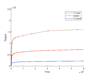
Figure 1: Convergence of the algorithm in the setup of [38]. $L=50,c_{3}(k)=1.8^{k}$.

Further simulations are provided in Appendix 6.1.

6 Conclusion

Fair division of resources is a highly desired goal in designing machine learning algorithms. In this paper, we presented a multi-agent bandit algorithm solving the max-min fair bandit problem with a near logarithmic regret order and polynomial complexity in the number of agents. The paper brings new ideas from distributed computation into the world of online multi-agent learning. Comparison to state-of-the-art is significantly favorable. We also comment that when there are more agents than arms, the techniques of [24] might be useful for arm sharing.

6.1 Simulations for various number of agents

To demonstrate the scalability of the algorithm, we present 100 Monte-Carlo experiments for $N=2,4,8,16,32,64\hbox{\ and \ }128$ agents. The minimal gap was $\frac{1}{N}$, by selecting the arm values for each agent as a random permutation of the numbers $\frac{k}{N}:k=1,\ldots,N$. The number of epochs was set to 32. We can clearly see the logarithmic dependence of the cumulative regret on $T$ for each value of $N$, as well as the polynomial dependence on the number of agents.

Figure 2 presents the median regret over $100$ Monte-Carlo tests as a function of time on a logarithmic scale. We can clearly see the near linear growth with $\log T$ for various numbers of agents. Figure 3 presents the median regret at various points in time as a function of the number of agents over $100$ Monte-Carlo tests. We can see that the regret grows approximately linearly with time.

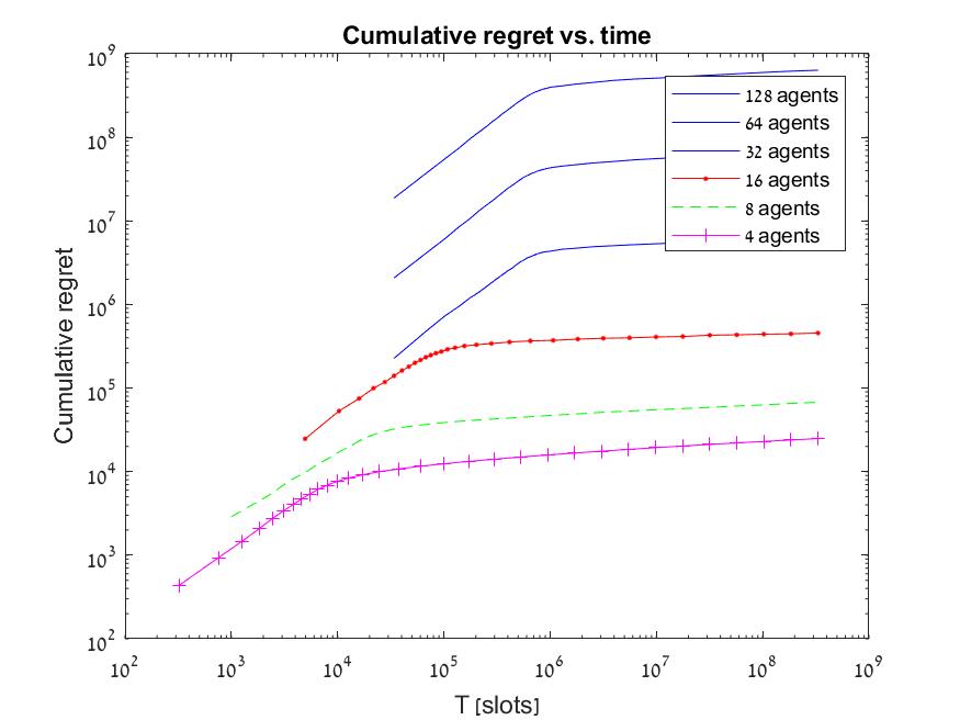
Figure 2: Evolution of the regret vs. time.

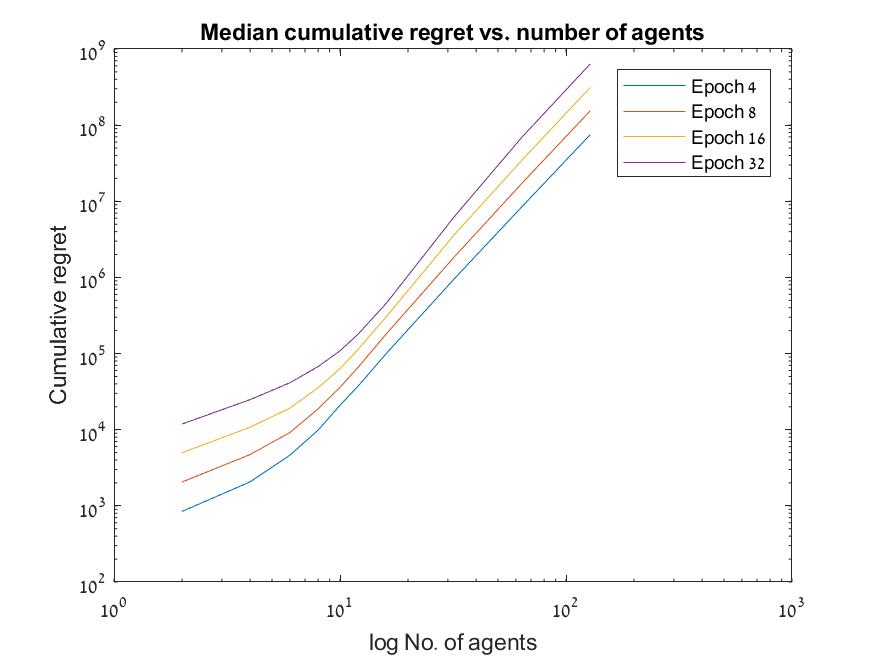
Figure 3: Evolution of the regret vs. number of agents.

Appendix A Proof of Lemma 4.2

First we compute the probability that our overestimate of the support of one of the arm fails. Let

$$\gamma =max_{m,n}F(B_{m,n}/2)$$ (22)

$$\mbox{${\hat{B}}$}(K) =max_{m,n}\mbox{${\hat{B}}$}_{m,n}(K).$$ (23)

By definition of the support $B_{m,n}$ we must have $\gamma<1$. Hence $P_{1}=P\left(\exists m,n:\mbox{${\hat{B}}$}_{m,n}(K)<B_{m,n}\right)<\gamma^{\ell_{K}}$. Let $\small{P_{2}=P\left(\exists n,m:\left|\mbox{${\hat{R}}$}_{n,m}(K)-R_{n,m}\right|>\delta\left|\mbox{${\hat{B}}$}(K)>B\right.\right)}$

$$\small{P\left(\exists n,m:\left|\mbox{${\hat{R}}$}_{n,m}(K)-R_{n,m}\right|>\delta\right)<P_{1}+P_{2}}$$

$$<NM\left(\gamma^{\ell_{K}}+2e^{-2\frac{\ell_{K}\delta^{2}}{\mbox{${\hat{B}}$}(K)^{2}}}\right).$$

The first term follows from Lemma 3.1 and a union bound while the second from Hoeffding bound and the condition $B<\mbox{${\hat{B}}$}(K)<2B$. By (7), $\ell_{K}=LKf(K)$. $f(k)$ is diverging and $\gamma<1$ so there is a $k_{0}$ sufficiently large such that $\forall k\geq k_{0}\quad\gamma^{f(k)}<1/2$ and $f(k)\geq\ln 2(2B^{2}$+1).

$$P\left(\exists n,m:\left|\mbox{${\hat{R}}$}_{n,m}(k)-R_{n,m}\right|>\delta\right)<NM2^{-Lk(1+\delta^{2})}.$$ (24)

Appendix B Proof of Lemma 4.3

We can write for all $n,i,j$:

$$|(\mbox{${\hat{R}}$}_{n,i}-\mbox{${\hat{R}}$}_{n,j})| =|(\mbox{${\hat{R}}$}_{n,i}-R_{n,i})-(\mbox{${\hat{R}}$}_{n,j}-R_{n,j})$$

$$+(R_{n,j}-R_{n,i})|$$

$$\leq|\mbox{${\hat{R}}$}_{n,i})-R_{n,i}|+|\mbox{${\hat{R}}$}_{n,j}-R_{n,j}|$$

$$+|R_{n,j}-R_{n,i}|.$$ (25)

Therefore, minimizing (B) with respect to $n,i,j$ we obtain

$$\Delta\mbox{${\mathbf{\hat{R}}}$}\leq\Delta\mbox{${\mathbf{R}}$}+\min_{n}\min_{i\neq k}|\mbox{${\hat{R}}$}_{n,i}-R_{n,i}|+|\mbox{${\hat{R}}$}_{n,j}-R_{n,j}|.$$ (26)

Similar argument yields

$$\left|\Delta\mbox{${\mathbf{R}}$}-\Delta\mbox{${\mathbf{\hat{R}}}$}\right|\leq\min_{n}\min_{i\neq j}|\mbox{${\hat{R}}$}_{n,i}-R_{n,i}|+|\mbox{${\hat{R}}$}_{n,j}-R_{n,j}|.$$ (27)

Using assumption (16) we obtain

$$\left|\Delta(\mbox{${\mathbf{R}}$})-\Delta(\mbox{${\mathbf{\hat{R}}}$})\right|<\Delta(\mbox{${\mathbf{R}}$})/2.$$ (28)

Consider the agent, with the worst arm $i$ under the min-max allocation when using ${\mathbf{R}}$. By (28), the gap between any two arms for each user is no larger than $\Delta\mbox{${\mathbf{R}}$}/2$. Hence changing ${\mathbf{R}}$ to ${\mathbf{\hat{R}}}$ the min-max arm must remain the same, since switching will change the reward by at least $\Delta\mbox{${\mathbf{R}}$}$, while each arm did not change by more than $\Delta\mbox{${\mathbf{R}}$}/2$. Similarly, if an agent had a reward above the max-min value, it cannot become the new maxmin value, since its reward under ${\mathbf{\hat{R}}}$ cannot change by more than $\Delta\mbox{${\mathbf{R}}$}/2$, thus it cannot become lower then the previous worst arm. ∎

Appendix C Pseudo code for the proposed algorithm

We present the detailed pseudo-code of the proposed Algorithm 1.. The general structure is an agent ordering Algorithm C.1 followed by epochs each consisting of three phases. The length of each phase is determined as described in the paper. The subsequent sub-sections describe the phases. Exploration is described in Appendix C.2. Finally, the matching phase and the implementation of the distributed auction is described in Appendix C.3.

C.1 Agent Ordering

The agent ordering phase is performed approximately, $\beta N\log_{2}(N)$ steps. It ends when each agent $n$ has been assigned a unique number $i_{n}$, $1\leq i_{n}\leq N$. The algorithm is presented in Algorithm 2.

1:  Initialization

2:  endflag $\leftarrow 0$.

3:  Each agent $n$ sets:

4:  $s_{n}\leftarrow$ unassigned.

5:  Set arm $m$ available $\leftarrow 1$, $m=1,\ldots,N$.

6:  Note that we only need the first $N$ arms for ordering.

7:  while endflag=0 do

8:     even collison flag $\leftarrow 0$.

9:     for $t=0,\ldots 4N\log_{2}(N)-1$ do

10:        if $t$ is even then

11:           if $s_{n}=$ unassigned then

12:              Randomly select available arm $m_{n}(t)$.

13:              Sample arm $m_{n}(t)$.

14:              if $r_{n,m_{n}(t)}\neq 0$ then

15:                 $s_{n}\leftarrow$ assigned.

16:                 $i_{n}=m(t)$.

17:              end if

18:           else

19:              sample arm $i_{n}$.

20:           end if

21:        else

22:           if $s_{n}=$ unassigned then

23:              Sample again arm $m(t-1)$.

24:              if $r_{n,m(t-1)}\neq 0$ then

25:                 arm $m(t-1)$ $\leftarrow$ unavailable.

26:              end if

27:           end if

28:        end if

29:     end for

30:     for $t=1:N$ do

31:        if $s_{n}=$unassigned then

32:           Sample arm $t$.

33:        else

34:           if $t=i_{n}$ then

35:              Sample arm $i_{n}$.

36:              if ${r_{n,m(t-1)}\neq 0}$ then

37:                 end flag $\leftarrow 1$.

38:              end if

39:           end if

40:        end if

41:     end for

42:  end while

43:  Output for agent $n$ is a number $1\leq i_{n}\leq N$.

Algorithm 2 Agent ordering(n)

C.2 Exploration

The algorithm Exploration$(k,n)$ is presented in Algorithm 3. As explained, the length of the exploration becomes constant as our estimate of the support of the distribution improves.

1:  Initialization

2:  Set exploration length $T_{\hbox{exploration}}.\leftarrow\mbox{${\hat{B}}$}(k-1)M+1$, where $\mbox{${\hat{B}}$}(k-1)$ is the estimate of the maximal support of the arm distributions.

3:  end of iterations $\leftarrow 0$

4:  for $t=1$ to $T_{\hbox{exploration}}$ and end of iterations$=0$ experienced do

5:     for $\ell=1$ to $L$ do

6:        $m=i_{n}+tL+\ell\mod M$ is the arm sampled by agent $n$ at time $t$.

7:        Agent $n$ samples arm $m$ obtaining $r_{m,n}(t)$.

8:        $\mbox{${\hat{R}}$}_{n,m}\leftarrow\frac{V_{n,m}}{V_{n,m}+1}\mbox{${\hat{R}}$}_{n,m}+\frac{1}{V_{n,m}+1}r_{m,n}(t)$.

9:        $V_{n,m}\leftarrow V_{n,m}+1$.

10:     end for

11:     end of iterations $\leftarrow 1$.

12:     for t=1:N do

13:        if agent $n$ did not finish $T_{\hbox{exploration}}$ rounds then

14:           Sample arm $m=t$.

15:        else

16:           Sample arm $m=i_{n}$.

17:        end if

18:        if $r_{n,m}(t)=0$ then

19:           end of iterations $\leftarrow 0$.

20:        end if

21:     end for

22:  end for

23:  Output:

24:  $\mbox{${\hat{R}}$}_{n,m},m=1,\ldots,M$.

Algorithm 3 Exploration$(k,n)$

C.3 Matching

The matching phase includes a binary search for the max-min value as described in Algorithm 4, which is composed of a sequence of searches for a matching with value $\tau$ or above. Each search for a matching implements the distributed auction for maximum cardinality matching, where each agent keeps it local prices as described in Algorithm 5.

1:  Input:

2:  $\mbox{${\hat{R}}$}_{n,m},m=1,\ldots,M$.

3:  Initialization

4:  $\tau_{\min}\leftarrow 0,\tau_{\max}\leftarrow 1,\tau=1$.

5:  $\Delta_{n}\leftarrow\min_{i\neq j}\left|\mbox{${\hat{R}}$}_{n,i}-\mbox{${\hat{R}}$}_{n,j}\right|/4$.

6:  Infeasible flag $\leftarrow 0$.

7:  for $m=1,\ldots M$ do

8:     if $\mbox{${\hat{R}}$}_{n,m}\geq\tau$ then

9:        $A_{n,m}(\tau)\leftarrow 1$

10:     else

11:        $A_{n,m}(\tau)\leftarrow 0$

12:     end if

13:  end for

14:  Allocation$(n),i_{ind}\leftarrow 0$

15:  while Infeasible flag $=0$ or $\Delta_{n}<\tau_{\max}-\tau_{min}$ or Allocation$(n)=0$ or $i_{ind}<LK$ do

16:     $i_{ind}\leftarrow i_{ind}+1$

17:     $\pi_{n}\leftarrow$ Distributed auction$(A_{n}(\tau))$.

18:     if $\pi_{n}=0$ then

19:        infeasible flag $\leftarrow 1$.

20:        $\tau_{max}\leftarrow\tau$.

21:     else

22:        $\tau_{min}\leftarrow\tau$.

23:        Allocation$(n)\leftarrow\pi_{n}$.

24:     end if

25:     $\tau\leftarrow 0.5(\tau_{\max}+\tau_{\min})$.

26:  end while

27:  Output:

28:  Allocation$(n)$.

Algorithm 4 Distributed matching phase(n)

1:  Input:

2:  $A_{n,m},m=1,\ldots,M$.

3:  Initialization

4:  Assigned$(n)\leftarrow 0$.

5:  for $m=1,\dots,M$ do

6:     if $A_{n,m}=1$ then

7:        $h_{m}\leftarrow 0$

8:     else

9:        $h_{m}\leftarrow\infty$

10:     end if

11:  end for

12:  for $t=1,\ldots N^{2}(N-1)$ do

13:     if Assigned$(n)=1$ then

14:        Access arm $\pi(n)$.

15:        if $r_{n,\pi(n)}=0$ then

16:           Assigned$(n)\leftarrow 0$.

17:           $h_{n,\pi(n)}\leftarrow h_{\pi(n)}+1$.

18:           $\pi(n)=0$.

19:        end if

20:     else

21:        if $t=i_{n}\mod N$ then

22:           $\pi(n)\leftarrow\arg\min_{m}h_{n,m}$

23:           Access arm $\pi(n)$.

24:           Assigned$(n)\leftarrow 1$.

25:        end if

26:     end if

27:  end for

28:  for $t=1,\ldots,N$ do

29:     if Assigned$(n)=0$ then

30:        Access arm $t$

31:     else

32:        if $t=\pi(n)$ then

33:           Access arm $\pi(n)$

34:           if $r_{n,\pi(n)}=0$ then

35:              $\pi(n)\leftarrow 0$

36:           end if

37:        end if

38:     end if

39:  end for

40:  Output: $\pi(n)$. Note that $\pi(n)=0$, implies there is no perfect matching.

Algorithm 5 Distributed auction(n)

References

- [1] I. Bistritz and A. Leshem, “Distributed multi-player bandits-a game of thrones approach,” in Advances in Neural Information Processing Systems, pp. 7222–7232, 2018.
- [2] K. Liu and Q. Zhao, “Distributed learning in multi-armed bandit with multiple players,” IEEE Transactions on Signal Processing, vol. 58, no. 11, pp. 5667–5681, 2010.
- [3] J. Xu, C. Tekin, S. Zhang, and M. Van Der Schaar, “Distributed multi-agent online learning based on global feedback,” IEEE Transactions on Signal Processing, vol. 63, no. 9, pp. 2225–2238, 2015.
- [4] S. Vakili, K. Liu, and Q. Zhao, “Deterministic sequencing of exploration and exploitation for multi-armed bandit problems,” IEEE Journal of Selected Topics in Signal Processing, vol. 7, no. 5, pp. 759–767, 2013.
- [5] L. Lai, H. Jiang, and H. V. Poor, “Medium access in cognitive radio networks: A competitive multi-armed bandit framework,” in Signals, Systems and Computers, 2008 42nd Asilomar Conference on, pp. 98–102, 2008.
- [6] A. Anandkumar, N. Michael, A. K. Tang, and A. Swami, “Distributed algorithms for learning and cognitive medium access with logarithmic regret,” IEEE Journal on Selected Areas in Communications, vol. 29, no. 4, pp. 731–745, 2011.
- [7] L. T. Liu, H. Mania, and M. I. Jordan, “Competing bandits in matching markets,” arXiv preprint arXiv:1906.05363, 2019.
- [8] H. Liu, K. Liu, and Q. Zhao, “Learning in a changing world: Restless multiarmed bandit with unknown dynamics,” IEEE Transactions on Information Theory, vol. 59, no. 3, pp. 1902–1916, 2013.
- [9] O. Avner and S. Mannor, “Concurrent bandits and cognitive radio networks,” in Joint European Conference on Machine Learning and Knowledge Discovery in Databases, pp. 66–81, 2014.
- [10] N. Nayyar, D. Kalathil, and R. Jain, “On regret-optimal learning in decentralized multiplayer multiarmed bandits,” IEEE Trans. Control Netw. Syst., vol. 5, no. 1, pp. 597–606, 2016.
- [11] N. Evirgen and A. Kose, “The effect of communication on noncooperative multiplayer multi-armed bandit problems,” in arXiv preprint arXiv:1711.01628, 2017, 2017.
- [12] J. Cohen, A. Héliou, and P. Mertikopoulos, “Learning with bandit feedback in potential games,” in Proceedings of the 31th International Conference on Neural Information Processing Systems, 2017.
- [13] O. Avner and S. Mannor, “Multi-user lax communications: a multi-armed bandit approach,” in INFOCOM 2016-The 35th Annual IEEE International Conference on Computer Communications, IEEE, pp. 1–9, 2016.
- [14] S. Zafaruddin, I. Bistritz, A. Leshem, and D. Niyato, “Distributed learning for channel allocation over a shared spectrum,” IEEE J. Sel. Areas Commun., vol. 37, no. 10, pp. 2337–2349, 2019.
- [15] M. K. Hanawal and S. J. Darak, “Multi-player bandits: A trekking approach,” arXiv preprint arXiv:1809.06040, 2018.
- [16] I. Bistritz and N. Bambos, “Cooperative multi-player bandit optimization,” Advances in Neural Information Processing Systems, vol. 33, 2020.
- [17] J. Rosenski, O. Shamir, and L. Szlak, “Multi-player bandits–a musical chairs approach,” in International Conference on Machine Learning, pp. 155–163, 2016.
- [18] E. Boursier and V. Perchet, “Sic-mmab: Synchronisation involves communication in multiplayer multi-armed bandits,” in Adv Neural Inf Process Syst., pp. 12048–12057, 2019.
- [19] P. Alatur, K. Y. Levy, and A. Krause, “Multi-player bandits: The adversarial case,” J. Mach. Learn. Res., vol. 21, no. 77, pp. 1–23, 2020.
- [20] S. Bubeck, Y. Li, Y. Peres, and M. Sellke, “Non-stochastic multi-player multi-armed bandits: Optimal rate with collision information, sublinear without,” arXiv preprint arXiv:1904.12233, 2019.
- [21] S. Bubeck, N. Cesa-Bianchi, et al., “Regret analysis of stochastic and nonstochastic multi-armed bandit problems,” Foundations and Trends® in Machine Learning, vol. 5, no. 1, pp. 1–122, 2012.
- [22] O. Naparstek and A. Leshem, “Fully distributed optimal channel assignment for open spectrum access,” IEEE Trans. Signal Process., vol. 62, no. 2, pp. 283–294, 2014.
- [23] Q. Zhao and L. Tong, “Opportunistic carrier sensing for energy-efficient information retrieval in sensor networks,” EURASIP J. Wirel. Commun. Netw., vol. 2005, no. 2, pp. 1–11, 2005.
- [24] T. Boyarski, W. Wang, and A. Leshem, “Distributed learning for optimal spectrum access in dense device-to-device ad-hoc networks,” IEEE Transactions on Signal Processing, 2023.
- [25] L. Besson and E. Kaufmann, “Multi-player bandits revisited,” in Algorithmic Learning Theory, pp. 56–92, 2018.
- [26] H. Tibrewal, S. Patchala, M. K. Hanawal, and S. J. Darak, “Distributed learning and optimal assignment in multiplayer heterogeneous networks,” in IEEE INFOCOM 2019-IEEE Conference on Computer Communications, pp. 1693–1701, IEEE, 2019.
- [27] I. Bistritz and A. Leshem, “Game of thrones: Fully distributed learning for multiplayer bandits,” Mathematics of Operations Research, vol. 46, no. 1, pp. 159–178, 2021.
- [28] D. Kalathil, N. Nayyar, and R. Jain, “Decentralized learning for multiplayer multiarmed bandits,” IEEE Transactions on Information Theory, vol. 60, no. 4, pp. 2331–2345, 2014.
- [29] A. Mehrabian, E. Boursier, E. Kaufmann, and V. Perchet, “A practical algorithm for multiplayer bandits when arm means vary among players,” in 23rd AISTATS, (online), pp. 1211–1221, PMLR, Aug. 2020.
- [30] J. F. Nash Jr, “The bargaining problem,” Econometrica: Journal of the econometric society, pp. 155–162, 1950.
- [31] W. Kubiak, Proportional optimization and fairness, vol. 127. Springer Science & Business Media, 2008.
- [32] E. Kalai and M. Smorodinsky, “Other solutions to nash’s bargaining problem,” Econometrica: Journal of the Econometric Society, pp. 513–518, 1975.
- [33] K. M. Mjelde, “Properties of pareto optimal allocations of resources to activities,” modeling, identification and control, vol. 4, no. 3, pp. 167–173, 1983.
- [34] E. Zehavi, A. Leshem, R. Levanda, and Z. Han, “Weighted max-min resource allocation for frequency selective channels,” IEEE transactions on signal processing, vol. 61, no. 15, pp. 3723–3732, 2013.
- [35] B. Radunovic and J.-Y. Le Boudec, “A unified framework for max-min and min-max fairness with applications,” IEEE/ACM Transactions on networking, vol. 15, no. 5, pp. 1073–1083, 2007.
- [36] A. Asadpour and A. Saberi, “An approximation algorithm for max-min fair allocation of indivisible goods,” SIAM Journal on Computing, vol. 39, no. 7, pp. 2970–2989, 2010.
- [37] I. Bistritz, T. Baharav, A. Leshem, and N. Bambos, “My fair bandit: Distributed learning of max-min fairness with multi-player bandits,” in International Conference on Machine Learning, pp. 930–940, PMLR, 2020.
- [38] I. Bistritz, T. Z. Baharav, A. Leshem, and N. Bambos, “One for all and all for one: Distributed learning of fair allocations with multi-player bandits,” IEEE J. Sel. Areas Inf. Theory, vol. 2, no. 2, pp. 584–598, 2021.
- [39] S. J. Darak and M. K. Hanawal, “Multi-player multi-armed bandits for stable allocation in heterogeneous ad-hoc networks,” IEEE Journal on Selected Areas in Communications, vol. 37, no. 10, pp. 2350–2363, 2019.
- [40] Y. Bar-On and Y. Mansour, “Individual regret in cooperative nonstochastic multi-armed bandits,” in Adv Neural Inf Process Syst. (H. Wallach, H. Larochelle, A. Beygelzimer, F. d'Alché-Buc, E. Fox, and R. Garnett, eds.), vol. 32, pp. 3116–3126, Curran Associates, Inc., 2019.
- [41] S. Jabbari, M. Joseph, M. Kearns, J. Morgenstern, and A. Roth, “Fairness in reinforcement learning,” in Proceedings of the 34th International Conference on Machine Learning-Volume 70, pp. 1617–1626, JMLR. org, 2017.
- [42] M. Joseph, M. Kearns, J. H. Morgenstern, and A. Roth, “Fairness in learning: Classic and contextual bandits,” in Advances in Neural Information Processing Systems, pp. 325–333, 2016.
- [43] X. Zhang, M. Khaliligarekani, C. Tekin, et al., “Group retention when using machine learning in sequential decision making: the interplay between user dynamics and fairness,” Advances in neural information processing systems, vol. 32, 2019.
- [44] J. Mo and J. Walrand, “Fair end-to-end window-based congestion control,” IEEE/ACM Transactions on networking, no. 5, pp. 556–567, 2000.
- [45] T. L. Lai and H. Robbins, “Asymptotically optimal allocation of treatments in sequential experiments,” Design of Experiments: Ranking and Selection, pp. 127–142, 1984.
- [46] J. Katz-Samuels and K. Jamieson, “The true sample complexity of identifying good arms,” in International Conference on Artificial Intelligence and Statistics, pp. 1781–1791, 2020.
- [47] R. Rom and M. Sidi, Multiple access protocols: Performance and analysis. Springer Science & Business Media, 2012.
- [48] D. P. Bertsekas, “A distributed algorithm for the assignment problem,” Lab. for Information and Decision Systems Working Paper, MIT, 1979.
- [49] O. Naparstek and A. Leshem, “Expected time complexity of the auction algorithm and the push relabel algorithm for maximum bipartite matching on random graphs,” Random Structures & Algorithms, vol. 48, no. 2, pp. 384–395, 2016.
- [50] A. V. Goldberg and R. Kennedy, “An efficient cost scaling algorithm for the assignment problem,” Mathematical Programming, vol. 71, no. 2, pp. 153–177, 1995.
- [51] D. P. Bertsekas and D. A. Castanon, “A forward/reverse auction algorithm for asymmetric assignment problems,” Computational Optimization and Applications, vol. 1, pp. 277–297, 1992.
- [52] D. P. Bertsekas, “The auction algorithm: A distributed relaxation method for the assignment problem,” Annals of operations research, vol. 14, no. 1, pp. 105–123, 1988.