Evaluating the Impact of Regulatory Policies on Social Welfare in Difference-in-difference Settings

Abstract. Quantifying the impact of regulatory policies on social welfare generally requires the identification of counterfactual distributions. Many of these policies (e.g. minimum wages or minimum working time) generate mass points and/or discontinuities in the outcome distribution. Existing approaches in the difference-in-difference literature cannot accommodate these discontinuities while accounting for selection on unobservables and non-stationary outcome distributions. We provide a unifying partial identification result that can account for these features. Our main identifying assumption is the stability of the dependence (copula) between the distribution of the untreated potential outcome and group membership (treatment assignment) across time. Exploiting this copula stability assumption allows us to provide an identification result that is invariant to monotonic transformations. We provide sharp bounds on the counterfactual distribution of the treatment group suitable for any outcome, whether discrete, continuous, or mixed. Our bounds collapse to the point-identification result in Athey and Imbens (2006) for continuous outcomes with strictly increasing distribution functions. We illustrate our approach and the informativeness of our bounds by analyzing the impact of an increase in the legal minimum wage using data from a recent minimum wage study (Cengiz, Dube, Lindner, and Zipperer, 2019).

Keywords: Copula, Identified Set, Changes-in-Changes, Sharp bounds, Social welfare treatment effects.

JEL Classification: C12, C14, C21 and C26

1. Introduction

Government’s regulatory role and its impact on social welfare has been a critical question for economists. These regulatory policies often restrict the budget or choice sets for certain agents in the market by imposing floors or quotas, such as minimum wages, minimum/maximum working time, wage floors for different occupation groups, etc. Those types of policies tend to induce behavioral responses that can generate mass points in the outcome of interest. For instance, an important question in the labor economics literature is the effect of an increase or introduction of minimum wages on low-wage jobs or overall employment, see for instance Card and Krueger (1994), Neumark and Wascher (2008), Cengiz, Dube, Lindner, and Zipperer (2019), among many others. The figure below (taken from Cengiz, Dube, Lindner, and Zipperer (2019)) illustrates that an increase in the minimum wage will shift jobs that were previously paying below the minimum wage $MW$, and then will create “excess jobs” at and slightly above the minimum wage.

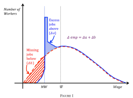
Figure 1. Figure 1 from Cengiz, Dube, Lindner, and Zipperer (2019)

This figure also shows the heterogeneous effect of such a policy, it is expected to only affect the wage of low-wage workers and not have an effect on the upper tail of the distribution. In sum, those types of policies have two main features. First, the potential outcomes of interest are likely to exhibit some mass points. Second, the causal effect of the policy is expected to affect only a part of the distribution of the outcomes of interest. As a result, to adequately analyze the impact of these policies, a distributional treatment effect analysis is key, as in Cengiz, Dube, Lindner, and Zipperer (2019) for instance; see, also, Almond, Hoynes, and Schanzenbach (2011); Assunção, McMillan, Murphy, and Souza-Rodrigues (2022). Furthermore, measuring the impact of such policies on social welfare requires recovering the counterfactual distribution of the outcome of interest.

While these types of policies are paramount in economics, the existing econometrics methods are not necessarily adequate to recover distributional causal effects in these settings. In the presence of data before and after a new policy, one of the most widely used techniques to assess its impact is the difference-in-differences (DiD) method. Its main drawbacks, however, are two-fold: (1) it does not identify the counterfactual distribution, (2) it is not invariant to monotonic transformations. While there are several methods extending DiD to identify the counterfactual distribution (Athey and Imbens, 2006; Bonhomme and Sauder, 2011; Callaway and Li, 2019; Havnes and Mogstad, 2015), to the best of our knowledge, the distributional DiD and changes-in-changes (CiC) are the only two approaches that are invariant to monotonic transformations.

Roth and Sant’Anna (2021) show that distributional DiD requires that the distribution of the untreated potential outcome is independent of policy adoption, is stationary across time (within each group), or consists of a mixture of two subpopulations each obeying one of these restrictions. Those restrictions are unlikely to be valid for the policy evaluation questions we are interested in. Indeed, the independence assumption (random assignment) is implausible in our context since the decision to implement a new minimum wage policy is a response to the unsatisfactory features of the pre-policy outcome distribution, such as large wage inequalities, high proportion of workers under poverty, etc. When the policy is not randomly assigned, the validity of the distributional DiD essentially rests on the stationarity assumption, which is restrictive in many practical settings.

While the CiC approach introduced in the seminal work by Athey and Imbens (2006) can accommodate endogenous policy (treatment) assignment as well as time-varying potential outcome distributions, their identification result does not apply to the case where the potential outcomes exhibit some mass points (mixed distributions), as in Figure 1. In fact, Athey and Imbens (2006) introduce the CiC approach for either continuous or discrete outcomes that are monotonic (time-varying) functions of a scalar unobservable with a time-invariant distribution across time. In sum, the CiC approach introduced in Athey and Imbens (2006) cannot be applied to evaluate the policies described above.

The current paper provides an alternative, unifying identification result that applies to any type of outcome distribution, is invariant to monotonic transformations, allows for endogeneity of the policy assignment, and does not restrict the evolution of the marginal distribution, nor treatment effect heterogeneity. Our identification result exploits the stability of the dependence (copula) between treatment assignment and the untreated potential outcome across time without imposing restrictions on the structural function that generates the potential outcomes. Exploiting this identifying assumption, we provide a unifying partial identification result for the counterfactual distribution of the treatment group. Our copula stability (CS) bounds apply to any type of outcome distribution, whether it is continuous, mixed, or discrete. Our bounds shrink to the point-identification result in Athey and Imbens (2006) for outcomes with continuous, strictly increasing distributions. Indeed, we show that in this case our copula stability assumption is equivalent to the CiC conditions.

Since the motivation behind policies, such as increases in the legal minimum wage, is often to reduce inequality and/or target a specific part of the outcome distribution, we introduce a broad class of social welfare treatment effect parameters that can accommodate the policymaker’s objective. While this class includes the average treatment effect on the treated (ATT) as a special case, the ATT corresponds to a social welfare function that is inequality-neutral and gives equal weight to all individuals in the population. As a result, if a policymaker is averse to inequality, then the ATT would be an inadequate causal parameter to judge the policy’s effectiveness. In general, the social welfare function adequate to evaluate a specific regulatory policy can be highly context-specific and may depend on the policymaker’s preference and/or objective. We therefore introduce a broad class of treatment effect parameters that take into account the policy objectives. This broad class specifically includes the class of generalized Gini social welfare functions (e.g. Mehran, 1976; Weymark, 1981). These social welfare functions can take into account measures of inequality by putting higher weight on individuals with lower-ranked outcomes. In addition, we include a class of parameters that can capture the welfare of individuals at the lower tail or a specific interquantile range of the distribution. Bounds on these social welfare treatment effect parameters can be easily computed using our bounds on the counterfactual distribution. We illustrate the usefulness of this broad class of parameters and compare it to the ATT in the context of our empirical application examining the impact of a minimum wage policy (Section 3).

Next, we examine the connection between our main identifying assumption and the parallel trends assumption required by DiD. The parallel trends assumption can be equivalently stated as a covariance stability assumption. It is specifically a time invariance assumption on the covariance between treatment assignment and the untreated potential outcome, whereas our assumption maintains the stability of the copula between these two variables. As a result, there are several differences between our copula stability assumption and covariance stability (parallel trends). First, the parallel trends assumption restricts the joint variability of treatment assignment and the untreated potential outcome over time, whereas our copula stability assumption only restricts their dependence structure. Second, while the parallel trends assumption restricts the evolution of the marginal distribution of the untreated potential outcome across time, copula stability does not restrict the evolution of the marginal distribution, nor treatment effect heterogeneity. Last but not least, parallel trends are not invariant to monotonic transformations except under strong conditions on heterogeneity (Roth and Sant’Anna, 2021). These conditions specifically rule out the existence of a subpopulation that selects into treatment based on unobservables and exhibits changes in its potential outcome distribution. By contrast, our copula stability condition does not rule out such a subpopulation.

Before we proceed, a comparison between our identifying assumption and some of the related approaches in the literature is warranted. Bonhomme and Sauder (2011) exploit a separable model of the potential outcome to identify the entire counterfactual distribution of the treatment group in a DiD design. By relying on restrictions on the outcome model, it is therefore similar in spirit to the identification approach in Athey and Imbens (2006). The identification results in Callaway and Li (2019) exploit a copula stability restriction but on different objects than the ones used in this paper. They require the copula between changes and levels of the untreated potential outcome to be invariant across time for the treatment group, while our copula stability assumption does not restrict the evolution of the marginal distribution of the untreated potential outcome (Remark 1). Furthermore, our approach can be applied to repeated cross-sections or panel data and only requires two time periods, whereas Callaway and Li (2019) require at least three periods of panel data.

We organize the rest of the paper as follows. Section 2 introduces the analytical framework, presents our main identification result, introduces the class of social welfare treatment effect parameters and discusses the structural underpinnings of our main identifying assumption. Section 3 provides an empirical illustration examining the impact of minimum wage increases on the wage distribution revisiting Cengiz, Dube, Lindner, and Zipperer (2019).

2. Analytical Framework and Main Identification Results

Following Abadie (2005), we consider the potential outcomes model with two groups and two periods:

$$\left\{\begin{array}[]{lcl}Y_{0}&=&Y_{00}\\ \\ Y_{1}&=&Y_{11}D+Y_{10}(1-D)\end{array}\right.$$ (2.4)

where $Y_{t}$ denotes the observed outcome at period $t$ and $Y_{td}$ denotes the potential outcome at period $t\in\{0,1\}$ and treatment status $d\in\{0,1\}$. In the two-group, two-period case, $D$ denotes both group membership and the treatment status in period 1.

We use the following shorthand notation: $p\equiv\mathbb{P}(D=1)$, $q=1-p$, $\overline{\mathbb{R}}\equiv\mathbb{R}\cup\{-\infty,\infty\}$, $RanH\equiv\{H(y):y\in\mathbb{R}\}$, $\overline{Ran}F\equiv RanF\cup\{\inf RanF,\sup RanF\}$, and $DomH$ denotes the domain of the function $H$. We consider the following mappings $Q^{\mathbb{T},-}_{X}:[0,1]\rightarrow\mathbb{T}$, and $Q^{\mathbb{T},+}_{X}:[0,1]\rightarrow\mathbb{T}$, where $Q^{\mathbb{T},-}_{X}(u)\equiv\inf\{x\in\mathbb{T}\cup\{\infty\}:F_{X}(x)\geq u\}$ for all $u\in[0,1]$, $Q^{\mathbb{T},+}_{X}(u)\equiv\sup\{x\in\mathbb{T}\cup\{-\infty\}:F_{X}(x)\leq u\}$ for all $u\in[0,1]$. We call $Q^{\mathbb{T},+}_{X}$ and $Q^{\mathbb{T},-}_{X}$ generalized quantile functions whenever $F_{X}(.)$ is a well-defined cumulative distribution function (cdf). We denote by $\mathbb{F}$ the space of all well-defined cdfs. $SuppX=\mathbb{X}$ denotes the support of $X$, and $\mathbb{X}_{s|d}$ denotes the support of $X_{s}|D=d$ for $d\in\{0,1\}$. Finally, we define $f(x-)\equiv\sup_{z<x}f(z)$.

Our main identification result relies on restrictions imposed on the dependence structure across time. To do so, we rely on copula theory. Copulas are functions that enable us to separate the marginal distributions from the dependence structure of a given multivariate distribution. In our context, we are interested in the subcopula between the untreated potential outcome and group membership across time. Working with copulas in our case will allow us to avoid restricting the marginal distribution of the potential outcomes across time. To fix ideas, let us first provide a formal definition of the (sub)copula.

Definition 1 (Nelsen (2006)).

A two-dimensional subcopula is a function $C$ with the following properties:

1. $DomC=S_{1}\times S_{2}$, where $S_{1}$ and $S_{2}$ are subsets of $[0,1]$ containing $0$ and $1$;

2. For all $u,u^{\prime}\in S_{1}$, and $v,v^{\prime}\in S_{2}$ such that $u\leq u^{\prime}$, and $v\leq v^{\prime}$, we have:

   $$C(u^{\prime},v^{\prime})+C(u,v)\geq C(u^{\prime},v)+C(u,v^{\prime});$$

3. $C(0,v)=C(u,0)=0$ for all $(u,v)\in S_{1}\times S_{2}$, and $C(1,v)=v$, $C(u,1)=u$ for all $(u,v)\in S_{1}\times S_{2}$.

A copula is a special case of a subcopula where $S_{1}=S_{2}=[0,1]$. For a fixed $v\in S_{2}$, $u\mapsto C(u,v)$ is usually called the horizontal subcopula. The link between the joint distribution and the subcopula has been established by the well-known Sklar (1959) theorem, which provides the following lemma when applied to our context:

Lemma 1 (Sklar, 1959).

There exists a unique subcopula $C:\overline{Ran}F_{Y_{td}}\times\{0,q,1\}\rightarrow[0,1]$ such that

$$\mathbb{P}(Y_{td}\leq y,D=0)=C_{Y_{td},D}(F_{Y_{td}}(y),q),\;\;\;\text{ for }y\in[-\infty,\infty].$$

We can now state our main identification assumption as follows.

Assumption 1 (Dependence stability).

We impose a stability restriction on the horizontal copula at q: $C_{Y_{00},D}(u,q)=C_{Y_{10},D}(u,q)$ for all $u\in[0,1]$.

Assumption 1 is the key assumption behind our identification approach. It requires the dependence structure between the distribution of the untreated potential outcome and group membership to be stable across time. One of the main advantages of using a copula restriction is its invariance property. Indeed, for any right-continuous function $g$, that is strictly increasing on $\mathbb{Y}_{td}$, we have:

$$C_{g(Y_{td}),D}(u,q)=C_{Y_{td},D}(u,q),\;\;\forall u\in RanF_{Y_{td}}.$$

This copula invariance property will ensure our main identification result is invariant to any strictly monotonic transformation.

Given the wide use of parallel trends assumptions in difference-in-differences settings, it is important to clarify the relationship between our copula stability assumption and the parallel trends assumption. The parallel trends assumption can be equivalently rewritten as a covariance stability assumption as we show in Section D of the online appendix,

$$\mathbb{E}[Y_{10}-Y_{00}|D=1]=\mathbb{E}[Y_{10}-Y_{00}|D=0]\iff Cov(Y_{00},D)=Cov(Y_{10},D).$$ (2.5)

This equivalence result provides, first, an intuition on why the parallel trends assumption is not invariant to a monotonic transformation since the covariance is not invariant to a monotonic transformation. Second, it allows us to observe that the parallel trends assumption jointly restricts the evolution of the marginal distribution of $Y_{t0}$ across time and the dependence between $Y_{t0}$ and $D$. Unlike the parallel trends assumption, our copula stability assumption does not constrain the evolution of the marginal distribution across time, yet it relies only on the stability of the horizontal copula that governs the relationship between $Y_{t0}$ and $D$. As can be seen in the following equation, the two assumptions are non-nested in general:

$$Cov(Y_{td},D)=\int\left[C_{Y_{td,D}}(F_{Y_{td}}(y),q)-F_{Y_{td}}(y)q\right]dy.$$

Indeed, copula stability may hold while $Cov(Y_{10},D)\neq Cov(Y_{00},D)$ because $F_{Y_{10}}\neq F_{Y_{00}}$; and the covariance stability may hold while the copula stability is violated. We illustrate this in the following example.

Example 1.

Consider the following data generating process (DGP) in which the treatment is received when its gain (treatment effect) is bigger than or equal to a threshold, say 0 for simplicity. This is a simple Roy model where selection into treatment is on the gain.

$$\left\{\begin{array}[]{lcl}Y_{0}&=&U_{0}\\ \\ Y_{1}&=&\eta D+U_{1}\\ \\ D&=&\mathbbm{1}\{\eta\geq 0\}\end{array}\right.$$ (2.11)

where $\left(\begin{array}[]{c}U_{0}\\ U_{1}\\ \eta\end{array}\right)\sim N(0,\Sigma)$, $\Sigma=\left(\begin{array}[]{ccc}\sigma_{0}^{2}&\delta\sigma_{0}\sigma_{1}&\rho_{0}\sigma_{0}\\ \delta\sigma_{0}\sigma_{1}&\sigma_{1}^{2}&\rho_{1}\sigma_{1}\\ \rho_{0}\sigma_{0}&\rho_{1}\sigma_{1}&1\end{array}\right)$. In this case, we have the following:

1. Copula stability: $\rho_{0}=\rho_{1}\Leftrightarrow Corr(\eta,Y_{00})=Corr(\eta,Y_{10})$,

2. Parallel trends: $\rho_{0}\sigma_{0}=\rho_{1}\sigma_{1}\Leftrightarrow Cov(\eta,Y_{00})=Cov(\eta,Y_{10})$.

3. Distributional DiD: $\rho_{0}=\rho_{1}$ and $\sigma_{0}^{2}=\sigma_{1}^{2}$ $\Leftrightarrow$ $Y_{00}|D=d\sim Y_{10}|D=d$, for $d\in{0,1}$. We relegate the proof of all of the above statements to Appendix A.4.

As can be seen, the copula stability assumption is equivalent to $\rho_{0}=\rho_{1}$, meaning that the correlation between the policy effect $\eta$ and $Y_{t0}$ is stable over time. It does not restrict any moment of the marginal distribution of the potential outcomes $Y_{td}$. The parallel trends assumption, however, restricts the variances of the potential outcomes $Y_{00}$ and $Y_{10}$, since it is equivalent to $\rho_{0}\sigma_{0}=\rho_{1}\sigma_{1}$. The validity of the distributional DiD in this setting is implausible, since it requires stationarity of $Y_{t0}|D=d$. This could be easily checked using the observed distribution of the control group.

Remark 1.

Here, we formally compare our copula stability assumption with the one introduced in Callaway and Li (2019). To see this, let us define $\Delta Y_{t0}=Y_{t0}-Y_{(t-1)0}$, Callaway and Li (2019) require $C_{\Delta Y_{t0},Y_{(t-1)0}|D=1}(\cdot,\cdot)=C_{\Delta Y_{(t-1)0},Y_{(t-2)0}|D=1}(\cdot,\cdot)$. As can be seen, their assumption imposes a dependence stability on different objects than ours, and it requires at least three time periods of panel data. In addition, unlike us, their identification results require an additional independence condition between the change in the untreated potential outcome and treatment assignment, $\Delta Y_{t0}\perp D$.

Assumption 2 (Strictly increasing horizontal subcopula).

The function $u\mapsto C_{Y_{10},D}(u,q)$ is strictly increasing on $[0,1]$.

While Assumption 2 is less critical for our bounding approach, it allows us to significantly refine our bounds. It is essentially a restriction on the type of dependence between the potential outcomes and group membership. Many well-known parametric classes of copulas satisfy this assumption, e.g. Frank, Gumbel, Joe, or Gaussian copulas among many others. It excludes, however, extreme types of dependence captured by the Fréchet—Hoeffding copula bounds, i.e. $C(u,v)=\min\{u,v\}$ and $C(u,v)=\max\{u+v-1,0\}$. It is worth noting that this assumption is implied by some support conditions on the potential outcome distributions, as we show in the following result.

Lemma 2.

If $\mathbb{Y}_{t0|1}\subseteq\mathbb{Y}_{t0|0}$ then $u\mapsto C_{Y_{t0},D}(u,q)$ is strictly increasing on $RanF_{Y_{t0}}$, for $t\in\{0,1\}$

The main implication of the above lemma is that for continuous potential outcome distributions, i.e. $RanF_{Y_{t0}}=[0,1]$, the strict monotonicity of the copula (Assumption 2) is implied by a condition on the support of $Y_{td}$, $\mathbb{Y}_{t0|1}\subseteq\mathbb{Y}_{t0|0}$. That is, the support of the untreated potential outcome of the treatment group is included in the support of the untreated potential outcome of the control group. The support condition imposed in Athey and Imbens (2006) on the scalar unobservable in the CiC model implies this support condition on the untreated potential outcome.

We next state our main identification result:

Theorem 1.

Suppose that $\mathbb{Y}_{t0|1}\subseteq\mathbb{Y}_{t0|0}$ for $t\in\{0,1\}$, then under Assumptions 1 and 2, the bounds for the unobserved counterfactuals $F_{Y_{10}|D=1}(.)$ are:

$$\lim_{\tilde{y}\downarrow y}\sup\left\{F^{LB}(t):t\leq\tilde{y}\;\&\;t\in\mathbb{Y}_{10|0}\cup\{-\infty\}\right\}$$

$$\leq F_{Y_{10}|D=1}(y)$$

$$\leq \lim_{\tilde{y}\downarrow y}\sup\left\{F^{UB}(t):t\leq\tilde{y}\;\&\;t\in\mathbb{Y}_{10|0}\cup\{-\infty\}\right\}$$

for all $y\in\mathbb{R}$, where

$$F^{LB}(t) = F_{Y_{0}|D=1}\left(Q^{\mathbb{R},+}_{Y_{0}|D=0}\left(F_{Y_{1|D=0}}(y)\right)-\right)\;$$

$$\;F^{UB}(t) = F_{Y_{0}|D=1}\left(Q^{\mathbb{R},-}_{Y_{0}|D=0}\left(F_{Y_{1|D=0}}(y)\right)\right).$$

The above bounds are shown to be sharp when $\overline{Ran}F_{Y_{0}}$ is closed.

Theorem 1 provides a general (partial identification) result on the counterfactual distribution of the treatment group for any type of potential outcome variables (discrete, continuous, or mixed). Our result neither imposes any restriction on the heterogeneity of potential outcomes within a period nor across periods. We specifically do not impose restrictions on individual treatment effects i.e, $Y_{11}-Y_{10}$, or the evolution of the distribution of the untreated potential outcome across time, $F_{Y_{t0}},t\in\{0,1\}$. The formal proof is relegated to Appendix A. The derived bounds may look involved since we aim to provide a general formulation that covers any type of distribution and want to ensure that our bounds are indeed right-continuous. The bounds simplify for some special cases as we will illustrate in Corollary 1 below.

The intuition behind our (partial) identification result is very simple and can be summarized as follows: In the first period, we observe the joint distribution $\mathbb{P}(Y_{00}\leq y,D=0)$ and both marginal distributions, $\mathbb{P}(Y_{00}\leq y)$ and $q$. Using the Sklar result, we can recover the horizontal subcopula $C_{Y_{00},D}(u,q)$ on $RanF_{Y_{0}}$—the dependence structure in the first period. Then, since we assume the dependence structure to be stationary across time and we observe the joint distribution $\mathbb{P}(Y_{10}\leq y,D=0)$ in the second period, we can partially recover the marginal distribution $\mathbb{P}(Y_{10}\leq y)$. The main reason behind the partial identification is that in the first period we recover the subcopula $C_{Y_{00},D}(u,q)$ on $RanF_{Y_{0}}$ only and do not know the dependence structure outside this range. In the case of continuous potential outcomes, $RanF_{Y_{00}}=[0,1]$, our bounds shrink to a point because the first period allow us to recover the entire dependence structure that we carry out to the second period, as we show in the following corollary of Theorem 1.

Corollary 1.

Under Assumption 1, whenever $\mathbb{Y}_{t0|1}\subseteq\mathbb{Y}_{t0|0}$ for $t\in\{0,1\}$ and the cdfs $F_{Y_{t0}}(.)$, $t\in\{0,1\}$ are continuous and strictly increasing, we have:

$$F_{Y_{10}|D=1}(y)=F_{Y_{0}|D=1}\left(Q^{\mathbb{R},-}_{Y_{0}|D=0}\left(F_{Y_{1|D=0}}(y)\right)\right)$$

for all $y\in\mathbb{R}$.

Corollary 1 recovers the point-identification result obtained in Athey and Imbens (2006). Indeed, Athey and Imbens (2006) provide (partial) identification results for only two types of potential outcomes relying on different assumptions for each of the two cases: (i) continuous outcomes that are strictly monotonic in a scalar unobservable, (ii) discrete outcomes that are monotonic in a scalar unobservable. By contrast, Theorem 1 establishes a unifying identification result for any type of outcome under consideration. In addition to the connection to our identification result, there is a link between the CiC assumptions and our copula stability condition for continuous outcomes with strictly increasing cdfs. We provide the details on this connection in Section E of the online appendix.

Building on our unifying, partial identification result for the counterfactual distribution, we can now proceed to provide a class of policy-relevant parameters that quantify the impact of policy on social welfare in the entire population, subpopulations in the lower tail of the distribution or over any interquantile range of the distribution.

2.1. Policy-relevant parameters: Social welfare treatment effect on the treated (SWTT)

In general, when a policymaker decides to implement a new policy such as an increase in the legal minimum wage or legal minimum working time, she expects the policy to have a specific social welfare impact. The social welfare function used by the policymaker is not necessarily known to the researcher, however. For instance, the policymaker may consider social welfare functions that put more weight on specific subpopulations, such as lower-income individuals, or considers only social welfare functions with specific properties like social welfare functions that respect the Pigou-Dalton principle of transfers or the rank-dependent social welfare functions introduced by Mehran (1976).

As we will clarify below the widely used average treatment effect on the treated (ATT) corresponds to the case where the policymaker is inequality-neutral. If the policymaker is averse to inequality, however, the ATT would not be an adequate causal parameter to measure the impact of the policy or judge its effectiveness.

For this particular reason, we propose a novel class of parameters of interest that measure the causal effect of a particular policy in terms of a social welfare function,

$$SWTT_{\omega} \equiv SW_{\omega}(F_{Y_{11}|D=1})-SW_{\omega}(F_{Y_{10}|D=1}),$$

$$= \int_{0}^{1}\omega(\tau)\left(Q^{\mathbb{R},-}_{Y_{11}|D=1}(\tau)-Q^{\mathbb{R},-}_{Y_{10}|D=1}(\tau)\right)d\tau$$

where $SW_{\omega}(F_{X})=\int_{0}^{1}\omega(\tau)Q^{\mathbb{R},-}_{X}(\tau)$ denotes the social welfare function associated with a specific distribution $F_{X}$, and $\omega(\tau)\in[0,1]$ is a weighting function. This social welfare function can be alternatively viewed as a weighted average of the outcomes of individuals $i$ where the weights depend on the rank of $X_{i}$, $SW_{\omega}=\int{X_{i}\omega(Rank(X_{i}))}di$ (Kitagawa and Tetenov, 2021). Since the social welfare function essentially weights different quantiles of the distribution, the choice of the functional form of the weighting function relates to the inequality aversion of the policymaker and the extent thereof. We next consider several examples of weighting functions and discuss the properties of the social welfare functions they imply.

Before we proceed, it is important to emphasize that, while in many applications where measuring inequality is a concern, the outcome $Y$ is typically income or wages, our framework allows $Y$ to denote other outcomes as well as functions of different outcomes, such as consumption, income and/or human capital.

2.1.1. Generalized Gini social welfare function

The class of generalized Gini social welfare functions is the class of rank-dependent, equality-minded social welfare functions which satisfy the Pigou-Dalton principle of transfers and is given by

$$SW_{\Lambda}(F_{X})=\int{\Lambda(F_{X}(x))}dx.$$

where $\Lambda(\cdot):[0,1]\mapsto[0,1]$ is a convex, non-increasing, and non-negative function with boundary conditions $\Lambda(0)=1$ and $\Lambda(1)=0$. This class admits the equivalent representation as a weighted sum of quantiles with weighting function $\omega(\tau)=\frac{\partial(1-\Lambda(\tau))}{\partial\tau}$,

$$SW_{\Lambda}(F_{X}) = SW_{\omega}(F_{X})=\int{\omega(\tau)Q_{X}^{\mathbb{R},-}(\tau)}d\tau$$

As a result, the class of social welfare treatment effect parameters we introduce include this class as a special case. We proceed to present two important special cases of this class of social welfare functions, specifically the utilitarian and Gini social welfare functions.

Utilitarian welfare function

When $\omega(\tau)=1$, we have $SW_{\omega}(F_{X})=\int_{0}^{1}Q^{\mathbb{R},-}_{X}(\tau)d\tau$ $=\mathbb{E}[X].$ This corresponds to the additive welfare function and in this case our proposed parameter boils down to the ATT, i.e. $SWTT_{\omega}=ATT$. The ATT is therefore the appropriate parameter if the policymaker weights subpopulations at different quantiles of the distribution equally.

Gini social welfare function

When $\omega(\tau)=2(1-\tau)$, we have $SW_{\omega}(F_{X})=\int_{0}^{1}2(1-\tau)Q^{\mathbb{R},-}_{X}(\tau)d\tau=\mathbb{E}[X]\left(1-I_{Gini}(F_{X})\right),$ where $I_{Gini}(F_{X})\equiv\frac{\int_{0}^{1}(2\tau-1)Q^{\mathbb{R},-}_{X}(\tau)d\tau}{\mathbb{E}[X]}$ is the widely used Gini inequality index, see Sen (1974). $SW_{\omega}(F_{X})$ reflects the trade-off between the mean and (in)equality in the distribution $F_{X}$. The product $\mathbb{E}[X]I_{Gini}(F_{X})$ is a measure of the loss in social welfare due to inequality in the distribution $F_{X}$. In that case, $SWTT_{\omega}$ captures the impact of the policy using the Gini social welfare function, see Blackorby and Donaldson (1978) and Weymark (1981). In other words, if the policymaker implements the policy in order to reduce the level of inequality measured by the Gini index, this parameter is the most adequate to judge the impact of this policy.

Since $SW_{\omega}(F_{X})=\mathbb{E}[X]\left(1-I_{Gini}(F_{X})\right)$, we can decompose the $SWTT_{\omega}$ associated with the Gini social welfare function into a mean effect and an inequality effect as follows

$$SWTT_{\omega} = ~{}~{}~{}~{}~{}\underbrace{ATT(1-I_{Gini}(F_{Y_{11|D=1}}))}_{\text{Mean Component ($\Delta_{M}$)}}$$ (2.12)

$$-\underbrace{\mathbb{E}[Y_{10}|D=1](I_{Gini}(F_{Y_{11}|D=1})-I_{Gini}(F_{Y_{10}|D=1}))}_{\text{Inequality Component ($\Delta_{I}$)}}.$$

The first component consists of the product of the ATT and the deviation of the Gini coefficient for the potential outcome with the treatment from a Gini coefficient of 1, indicating a perfectly unequal distribution. Its sign is determined by the ATT, indicating that a positive ATT increases the Gini social welfare. The sign of the second component is determined by the difference in the Gini coefficient between the treated and untreated potential outcome distribution of the treatment group. Note that a reduction in inequality measured by the Gini coefficient increases the $SWTT_{\omega}$.

2.1.2. Second-order dominance

In many cases, when it is possible to do so, most inequality-averse policymakers like to rank distribution functions consistently with second-degree dominance. For instance, we say $F_{Y_{11}|D=1}$ second-order dominates $F_{Y_{10}|D=1}$ if and only if:

$$SWTT_{\omega}(u) \equiv SW_{\omega}(u,F_{Y_{11}|D=1})-SW_{\omega}(u,F_{Y_{10}|D=1})$$

$$= \int_{0}^{u}\left(Q^{\mathbb{R},-}_{Y_{11}|D=1}(\tau)-Q^{\mathbb{R},-}_{Y_{10}|D=1}(\tau)\right)d\tau\geq 0,$$

for all $u\in[0,1]$ and holds strictly for some $u$. In this special case, we have $\omega(\tau)=1\{\tau\leq u\}$. It is possible, however, that the observed and counterfactual distribution cannot be ranked using this criterion. Furthermore, the policy’s objective may be to reduce inequality in a specific part of the distribution. We therefore consider the following quantile-specific Gini social welfare functions.

2.1.3. Quantile-specific lower tail Gini social welfare function

In the Gini social welfare function discussed above, we assume that the policymaker is interested in the inequality of the whole population. Some policies may be concerned with reducing inequality up to specific quantiles of the distribution, however. To quantify the impact of the policy on lower-tail quantiles, we extend the quantile-specific lower-tail Gini social welfare measures introduced in Aaberge, Havnes, and Mogstad (2013) for continuous distributions to any type of distribution in order to accommodate the possibility of discontinuities resulting from censoring or bunching. To do so, we introduce the random variable $X^{u}=Q_{X}^{\mathbb{R},-}(V)$, where $V\sim\mathcal{U}[0,u]$ for $u\in(0,1]$. We relegate the derivations relevant to this section to Appendix A.5.

With this definition of $X^{u}$, we can show that the lower-tail Gini social welfare function can be decomposed into $\mathbb{E}[X^{u}]$ and the Gini coefficient associated with $F_{X^{u}}$ as follows

$$\int_{0}^{1}\frac{2}{u^{2}}(u-\tau)1\{\tau\leq u\}Q^{\mathbb{R},-}_{X}(\tau)d\tau=\mathbb{E}[X^{u}]\left(1-I_{Gini}(F_{X^{u}})\right),$$

where $I_{Gini}\left(F_{X^{u}}\right)\equiv\frac{\int_{0}^{1}(2\tau-u)1\{\tau\leq u\}Q^{\mathbb{R},-}_{X}(\tau)d\tau}{u^{2}\mathbb{E}[X^{u}]}$ is the lower-tail Gini coefficient at $u$ defined in Aaberge, Havnes, and Mogstad (2013). Therefore, $SWTT_{\omega}$ with $\omega(\tau)=\frac{2}{u^{2}}(u-\tau)1\{\tau\leq u\}$ yields the following,

$$SWTT_{\omega}(u) = \int_{0}^{u}\frac{2}{u^{2}}(u-\tau)\left(Q^{\mathbb{R},-}_{Y_{11}|D=1}(\tau)-Q^{\mathbb{R},-}_{Y_{10}|D=1}(\tau)\right)d\tau,$$

and is interpreted as the Quantile-$u$ lower tail Gini social welfare treatment effect on the treated.

Similar to the Gini social welfare, we can decompose the quantile-specific lower-tail Gini $SWTT_{\omega}(u)$ into a mean and inequality component,

$$SWTT_{\omega}(u) = ~{}~{}~{}\underbrace{ATT(u)(1-I_{Gini}(F_{Y_{11}^{u}|D=1}))}_{\Delta_{M}(u)}$$ (2.13)

$$-\underbrace{\mathbb{E}[Y_{10}^{u}|D=1](I_{Gini}(F_{Y_{11}^{u}|D=1})-I_{Gini}(F_{Y_{10}^{u}|D=1}))}_{\Delta_{I}(u)}.$$

where $ATT(u)=\mathbb{E}[Y_{11}^{u}-Y_{10}^{u}|D=1]$. As we demonstrate in our empirical application in Section 3, these quantities can shed light on the impact of policies that target the lower tail of the distribution, such as the minimum wage.

2.1.4. Interquantile Gini social welfare function

Since policies may target other parts of the distribution, such as the upper tail, we can generalize these quantile-specific social welfare treatment effect measures to any range of quantiles $[\underline{u},\overline{u}]$ a researcher may be interested in. Specifically, let $\underline{u}\in[0,1]$, $\overline{u}\in[0,1]$, $\underline{u}<\overline{u}$, $V\sim\mathcal{U}[\underline{u},\overline{u}]$, and $X^{\underline{u},\overline{u}}=Q_{X}^{\mathbb{R},-}(V)$. A derivation of $F_{X^{\underline{u},\overline{u}}}$ is relegated to Appendix A.5. Now by letting $\omega(\tau)=\frac{2}{(\overline{u}-\underline{u})^{2}}(\overline{u}-\tau)1\{\underline{u}<\tau\leq\overline{u}\}$, we obtain the Gini social welfare function specific to the quantile range $[\underline{u},\overline{u}]$,

$$SW_{\omega}(\underline{u},\overline{u})=\int_{0}^{1}\frac{2}{(\overline{u}-\underline{u})^{2}}(\overline{u}-\tau)1\{\underline{u}<\tau\leq\overline{u}\}Q_{X}^{\mathbb{R},-}(\tau)d\tau=\mathbb{E}[X^{\underline{u},\overline{u}}](1-I_{Gini}(F_{X^{\underline{u},\overline{u}}})),$$

where $\mathbb{E}[X^{\underline{u},\overline{u}}]\equiv\int_{\underline{u}}^{\overline{u}}Q_{X}^{\mathbb{R},-}(\tau)d\tau$ and $I_{Gini}\left(F_{X^{\underline{u},\overline{u}}}\right)\equiv\frac{\int_{0}^{1}(2\tau-\underline{u}-\overline{u})1\{\underline{u}<\tau\leq\overline{u}\}Q_{X}^{\mathbb{R},-}(\tau)d\tau}{(\overline{u}-\underline{u})^{2}\mathbb{E}[X^{\underline{u},\overline{u}}]}$. The interquantile Gini social welfare treatment effect on the treated over $[\underline{u},\overline{u}]$ is given by

$$SWTT_{\omega}(\underline{u},\overline{u}) \equiv SW_{\omega}(\underline{u},\overline{u},F_{Y_{11}|D=1})-SW_{\omega}(\underline{u},\overline{u},F_{Y_{10}|D=1})$$

$$= \int_{\underline{u}}^{\overline{u}}\frac{2}{(\overline{u}-\underline{u})^{2}}(\overline{u}-\tau)\left(Q^{\mathbb{R},-}_{Y_{11}|D=1}(\tau)-Q^{\mathbb{R},-}_{Y_{10}|D=1}(\tau)\right)d\tau.$$

2.2. Structural underpinnings of the copula stability assumption

Consider a policymaker who wants to implement a policy in a specific region, i.e. introduction/increase of a minimum wage. The policymaker decides to implement a policy if the gain in social welfare under the policy is higher than the gain in social welfare without the policy. The gain is evaluated by the policymaker given her information set $\mathcal{I}$. This decision rule is modeled as:

$$D = \mathbbm{1}\left\{\mathbb{E}[W(Y_{11})-W(Y_{00})|\mathcal{I}]>\mathbb{E}[W(Y_{10})-W(Y_{00})|\mathcal{I}]\right\},$$

$$= \mathbbm{1}\left\{\mathbb{E}[W(Y_{11})|\mathcal{I}]>\mathbb{E}[W(Y_{10})|\mathcal{I}]\right\}$$

where $\mathcal{I}$ is the sigma-algebra characterizing the decision maker information set at the time of the decision, $Y_{td}$ for $t,d\in\{0,1\}$ are $\mathcal{I}$ measurable. $W(.)$ is a measurable function that depends on the type of social welfare the policymaker wants to use. $W(.)$ can be specified to capture various types of societal welfare, like those discussed in the previous subsection.

To mimic our empirical illustration, we are considering the case where the outcomes of interest are mixed random variables because of the pre-existing minimum wage. We consider a general case where a minimum wage $\underline{w}_{0}$ exists in the pre-treatment period and the policymaker is considering an increase in this minimum wage, i.e. $\underline{w}_{1}>\underline{w}_{0}$.

$$Y_{t0} = Y^{\ast}_{t0}\mathbbm{1}\{Y^{\ast}_{t0}>\underline{w}_{0}\}+\underline{w}_{0}\mathbbm{1}\{Y^{\ast}_{t0}\leq\underline{w}_{0}\},~{}t=0,1,$$

$$Y_{11} = Y^{\ast}_{11}\mathbbm{1}\{Y^{\ast}_{11}>\underline{w}_{1}\}+\underline{w}_{1}\mathbbm{1}\{Y^{\ast}_{11}\leq\underline{w}_{1}\}.$$

Assume that $Z$ is a vector of random variables that is measurable with respect to the policymaker information $\sigma$-algebra $\mathcal{I}$, and $\mathbb{E}[W(Y_{1d})|\mathcal{I}]=\psi_{1d}(Z)+V_{1d}$, with $\mathbb{E}[V_{1d}|Z]=0$, where $V_{1d}$ for $d\in\{0,1\}$ are the prediction errors made by the policymaker given her information set. $Z$ could have a degenerate distribution and in such a case, the policymaker does not have additional information based on which she can form expectations. When $Z$ is observed by the econometrician, all our results hold conditional on $Z$.

In the following, we assume that $\zeta\equiv V_{10}-V_{11}$ and the latent variables have continuous distributions. Our model simplifies to:

$$\left\{\begin{array}[]{lcl}Y_{0}&=&Y_{00}\\ \\ Y_{1}&=&Y_{11}D+Y_{10}(1-D)\\ \\ D&=&\mathbbm{1}\left\{\psi_{11}(Z)-\psi_{10}(Z)\geq\zeta\right\}\end{array}\right.$$ (2.19)

Let $C_{Y^{\ast}_{t0},\zeta|Z=z}(u,v;\rho_{t}(z))$ be the conditional copula that captures the dependence between $Y^{\ast}_{t0}$ and $\zeta$. Suppose that $C_{Y^{\ast}_{t0},\zeta|Z=z}(u,v;\rho_{t}(z))$ belongs to the class of totally ordered copulas. Therefore, it can be shown that if $\rho_{0}(z)=\rho_{1}(z)$ —meaning that the dependence between the policymaker prediction errors $\zeta$ and $Y^{\ast}_{00}$ is the same as the dependence between $\zeta$ and $Y^{\ast}_{10}$, then the copula stability assumption holds conditional on $Z=z$, $C_{Y_{00},D|Z=z}(u,q)=C_{Y_{10},D|Z=z}(u,q)$ for all $u\in[0,1]$. A special case of this result is imposing a joint normal distribution on all the latent variables in the model such as

$$\left(\begin{array}[]{c}Y^{\ast}_{00}\\ Y^{\ast}_{10}\\ \zeta\end{array}\right)|Z=z\sim N(0,\Sigma),~{}\Sigma=\left(\begin{array}[]{ccc}\sigma_{0}^{2}(z)&\delta(z)\sigma_{0}(z)\sigma_{1}(z)&\rho_{0}(z)\sigma_{0}(z)\\ \delta(z)\sigma_{0}(z)\sigma_{1}(z)&\sigma_{1}^{2}(z)&\rho_{1}(z)\sigma_{1}(z)\\ \rho_{0}(z)\sigma_{0}(z)&\rho_{1}(z)\sigma_{1}(z)&1\end{array}\right)$$

.

In this case, copula stability conditional on $Z$ is equivalent to $\rho_{0}(z)=\rho_{1}(z)\Leftrightarrow Corr(\zeta,Y^{\ast}_{00}|Z=z)=Corr(\zeta,Y^{\ast}_{10}|Z=z)$, since the Gaussian copula belongs to the family of the strictly totally ordered copula. In this special case, our assumption is valid when the error of predictions made by the policymakers is correlated with the latent outcomes in the same way over time. The derivations relevant to this section are given in Appendix A.6.

3. Empirical Illustration

In this section, we illustrate the CS bounds revisiting the minimum wage study by Cengiz, Dube, Lindner, and Zipperer (2019). This application demonstrates the usefulness of the class of policy-relevant parameters we introduce to examine the impact of the minimum wage increase. In particular, the lower-tail quantile social welfare treatment effect estimates allow us to zoom into the lower tail of the distribution, where we expect the minimum wage to have an impact. Overall, our CS bounds document proportionately larger impacts on the Gini social welfare in the lowest part of the distribution, where the minimum wage increase led to increases in the mean and reductions in inequality in the lower tails. We also find that the distributional DiD exhibits violations of monotonicity in the lower tail of the distribution and is therefore not suitable for this application. In Section B.1 of the online appendix, we illustrate the CS bounds with another survey data set, revisiting the seminal work by Card and Krueger (1994).

Cengiz, Dube, Lindner, and Zipperer (2019) examine 138 prominent state-level minimum wage increases between 1979 and 2016 using the individual-level NBER-merged Outgoing Rotation Group Earnings Data of the Current Population Survey. Their goal is to examine the impact of the policy on the wage distribution around the minimum wage, as illustrated in Figure 1. In order to make the empirical illustration of the CS bounds in the context of this example succinct, we focus on two years, 2010 ($t=0$) and 2015 ($t=1$), and examine the distributional impact of a nontrivial minimum wage increase of $0.25 or more. Consistent with Section 2.2, we split our sample depending on the pre-treatment minimum wage. We specifically perform our analysis on two subgroups: (1) states with pre-treatment minimum wage below $8 (Subgroup 1), (2) states with pre-treatment minimum wage above or equal to $8 (Subgroup 2).

Table 1. Summary Statistics by Treatment and Control Groups

	Pre-treatment (2010)			Post-treatment (2015)
	Mean	S.D.	# Obs	Mean	S.D.	# Obs
Subgroup 1: States with Pre-Treatment Minimum Wage $<$ $8
Control	18.43	12.78	44,574	20.41	15.90	42,322
Treatment	20.20	14.26	38,261	22.12	18.21	32,489
Subgroup 2: States with Pre-Treatment Minimum Wage $\geq$ $8
Control	20.12	13.96	4,737	22.30	15.48	4,454
Treatment	23.13	17.42	19,877	25.83	18.74	18,039

Table 1 presents the summary statistics for hourly wage of both treatment and control groups before and after the treatment. For both subgroups, the summary statistics show that the mean and standard deviation is different across treatment and control groups within the same year as well as within groups across time.

3.1. Bounds on the counterfactual distribution

Figure 2 present the observed distribution of the treatment group in 2015, $\hat{F}_{Y_{1}|D=1}$, together with the CS bounds on the counterfactual distribution as well as its distributional DiD estimate for the bottom quartile of the wage distribution where the minimum wage increase is likely to have an impact.

Figure 2. Observed and Counterfactual Distributions: Bottom Quartile

Panel A. CS, Subgroup 1	Panel B. DistDiD, Subgroup 1
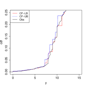
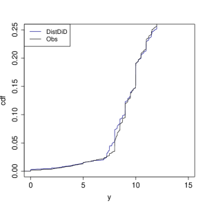
Panel C. CS, Subgroup 2	Panel D. DistDiD, Subgroup 2
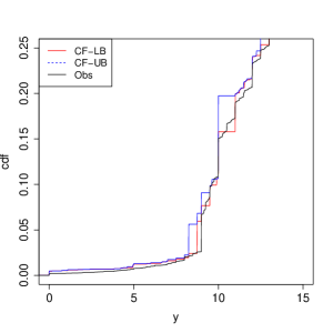
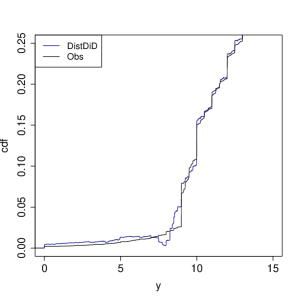
Notes: $Obs$ refers to the observed (factual) empirical outcome distribution of the treatment group $\hat{F}_{Y_{1}|D=1}$. $CF$-$LB$ ($CF$-$UB$) denotes the lower (upper) CS bound on $F_{Y_{10}|D=1}$, and $DistDiD$ refers to the distributional DiD estimate of $F_{Y_{10}|D=1}$. Subgroup 1 (Subgroup 2) refers to the subgroup of states with pre-treatment minimum wage of $<\$8$ ($\geq\$8$).

First, we examine the bottom quartile of the distributional DiD counterfactual for both subgroups (Panels B and D of Figure 2). At first glance, we note a clear violation of the monotonicity property of cdfs for Subgroup 2 (Panel D of Figure 2), indicating a violation of the testable implication of the identifying assumption of distributional DiD (Roth and Sant’Anna, 2021). In addition, the violation occurs around the pre-treatment minimum wage of $8, which is part of the distribution particularly pertinent for the evaluation of the minimum wage increase.

Table 2. Gini Social Welfare Treatment Effect Estimates

	$\hat{F}_{Y_{1}|D=1}$	SWTT
		CS-LB	CS-UB	DiD	DistDiD
Subgroup 1: States with Pre-treatment Minimum Wage $<$ $8
Mean ($ATT$)	22.12	-1.49	0.06	-0.06	-1.00
Gini SWF ($SWTT_{\omega}=\Delta_{M}-\Delta_{I}$)	14.53	-0.21	0.08	–	-0.08
Mean Component ($\Delta_{M}$)		-0.98	0.04	–	-0.65
Inequality Component ($\Delta_{I}^{\dagger}$)		-1.06	0.24	–	-0.58
Subgroup 2: States with Pre-treatment Minimum Wage $\geq$ $8
Mean ($ATT$)	25.83	0.12	0.56	0.53	-0.10
Gini SWF ($SWTT_{\omega}=\Delta_{M}-\Delta_{I}$)	16.89	0.06	0.36	–	0.25
Mean Component ($\Delta_{M}$)		0.08	0.37	–	-0.07
Inequality Component ($\Delta_{I}^{\dagger}$)		-0.28	0.30	–	-0.32
Notes: In order to understand the relative magnitude of the CS bounds, DiD and distributional DiD estimates, the column labeled $\hat{F}_{Y_{1}|D=1}$ reports the mean and Gini social welfare function of the observed (factual) distribution of the treatment group in 2015 ($t=1$). The definitions of the Gini $SWTT_{\omega}$, $\Delta_{M}$ and $\Delta_{I}$ are given in Section 2.1. †We emphasize that the bounds on $\Delta_{I}$ are outerset bounds.

Next, we examine the CS bounds on the counterfactual distribution (Panels A and C in Figure 2). Note that both upper and lower bounds satisfy the properties of a cdf. Furthermore, since the bounds do not cross, we do not have any detectable violation of our identifying assumption, unlike the distributional DiD. Comparing the observed (factual) distribution with the CS bounds on the counterfactual for both subgroups, we note an obvious change in the censoring point as expected in the context of a minimum wage increase. For instance, for Subgroup 1 (Panel A in Figure 2), both CS bounds on the counterfactual distribution exhibit a jump around the federal minimum wage of $7.25, albeit to varying degrees, whereas the observed (factual) distribution exhibits a jump around $8. Furthermore, for both subgroups (Panels A and C in Figure 2), the CS bounds differ from the observed (factual) distribution around the new minimum wage and below it, consistent with the conceptual framework in Cengiz, Dube, Lindner, and Zipperer (2019).

3.2. Bounds on treatment effects

Next, we quantify the impact of the minimum wage increase on the wage distribution using the ATT and the Gini social welfare treatment effects both for the overall distribution as well as its lower tail. We also present estimates of the parameters considered in Cengiz, Dube, Lindner, and Zipperer (2019). When comparing the distributional DiD estimates to the CS, it is important to keep in mind that the monotonicity violations we illustrate in Figure 2 are clear evidence against the identifying assumption of the distributional DiD in this empirical setting.

3.2.1. Overall social welfare treatment effects

Table 2 presents the CS bounds and the distributional DiD estimates for the ATT and the Gini social welfare treatment effect ($SWTT_{\omega}$). Before we proceed, we note that in order to facilitate the interpretation of the relative magnitude of the different treatment effect estimates, we report the mean and Gini social welfare function for $\hat{F}_{Y_{1}|D=1}$, the empirical outcome distribution of the treatment group in 2015 ($t=1$), in the first column of Table 2.

When examining Table 2, we first note that the ATT estimate obtained from the distributional DiD yields a very different estimate compared to the DiD for both subgroups, including a sign flip for Subgroup 2. This may be a consequence of the monotonicity violation we find in Figure 2. If taken at face value, both ATT estimates obtained from the distributional DiD suggest that the minimum wage increase reduced the average wage, with a nontrivial reduction of $1 for Subgroup 1. When examining the impact on the Gini social welfare, the distributional DiD suggests a small, but negative impact for Subgroup 1 and a positive impact for Subgroup 2.

Our CS bounds provide qualitatively different results. The CS bounds on the ATT and the Gini SWTT include zero, suggesting that the data is inconclusive on the sign of the effect of the minimum wage increase on the average wage and social welfare for Subgroup 1. As for Subgroup 2, our CS bounds on the ATT and the Gini SWTT suggest a small, positive impact on the average wage.

To aid in the interpretation of the impact on the Gini social welfare, Table 2 presents bounds on the mean and inequality components of the $SWTT_{\omega}$, introduced in Eq. (2.12) of Section 2.1,

$$SWTT_{\omega}=\Delta_{M}-\Delta_{I},$$

where $\Delta_{M}\equiv ATT(1-I_{Gini}(F_{Y_{11}|D=1}))$ captures the impact of the minimum wage increase on the mean and $\Delta_{I}\equiv\mathbb{E}[Y_{10}|D=1](I_{Gini}(F_{Y_{11}|D=1})-I_{Gini}(F_{Y_{10}|D=1})$ captures the impact on inequality. Note that a negative $\Delta_{I}$ implies a reduction in inequality, contributing to an increase in the Gini social welfare. The bounds on $\Delta_{M}$ can be obtained from scaling the bounds on the ATT by $(1-I_{Gini}(F_{Y_{11}|D=1}))$. We can provide outerset bounds on $\Delta_{I}$ relying on the CS bounds on SWTT_ω and $\Delta_{M}$. Let $\Delta_{M}^{LB}$ and $\Delta_{M}^{UB}$ ($SWTT_{\omega}^{LB}$ and $SWTT_{\omega}^{UB}$) denote the CS lower and upper bound for $\Delta_{M}$ ($SWTT_{\omega}$), respectively. Since $\Delta_{I}=\Delta_{M}-SWTT_{\omega}$, we construct outerset bounds on $\Delta_{I}$ using the following,

$$\Delta_{I}\in[\Delta_{M}^{LB}-SWTT_{\omega}^{UB},\Delta_{M}^{UB}-SWTT_{\omega}^{LB}].$$

While these bounds are valid, we emphasize, however, that they are not sharp.

The bounds on $\Delta_{M}$ and $\Delta_{I}$ in Table 2 suggest that for Subgroup 2 the positive impact on the Gini social welfare ($SWTT_{\omega}$) is driven by the mean component. For Subgroup 1, the bounds on the two components, $\Delta_{M}$ and $\Delta_{I}$, include zero, suggesting that we cannot identify the sign of either component similar to the $SWTT_{\omega}$ for this subgroup.

3.2.2. Lower-tail social welfare treatment effects

In the context of policies such as an increase in the legal minimum wage, the welfare of subpopulations at the lower tail of the wage distribution is an important policy target. Table 3 therefore provides the lower-tail ATT and Gini social welfare treatment effects, $ATT(u)$ and $SWTT_{\omega}(u)$, respectively, which we introduced in Section 2.1.3. We also provide bounds on the components of the $SWTT_{\omega}(u)$, specifically,

$$SWTT_{\omega}(u)=\Delta_{M}(u)-\Delta_{I}(u),$$

where $\Delta_{M}(u)\equiv ATT(u)(1-I_{Gini}(F_{Y_{11}|D=1}))$ and $\Delta_{I}(u)\equiv\mathbb{E}[Y_{10}^{u}|D=1](I_{Gini}(F_{Y_{11}^{u}|D=1})-I_{Gini}(F_{Y_{10}^{u}|D=1}))$. To obtain bounds on $\Delta_{M}(u)$, we scale the bounds on $ATT(u)$ by $(1-I_{Gini}(F_{Y_{11}^{u}|D=1}))$. As for $\Delta_{I}(u)$, we provide outerset bounds similar to those we construct for $\Delta_{I}$ in Table 2.

Table 3. Lower-Tail Quantile Social Welfare Treatment Effect Estimates

	Subgroup 1: States wit Pre-MW $<$ $8				Subgroup 2: States wit Pre-MW $\geq$ $8
	$\hat{F}_{Y_{1}|D=1}$	SWTT			$\hat{F}_{Y_{1}|D=1}$	SWTT
		CS-LB	CS-UB	DistDiD		CS-LB	CS-UB	DistDiD
Lower-tail Mean ($ATT(u)$)
$u=0.01$	2.37	0.47	0.55	0.44	3.63	1.59	1.68	1.90
$u=0.025$	4.45	0.15	0.29	0.13	6.15	0.95	1.06	1.06
$u=0.05$	6.14	0.24	0.44	0.13	7.57	0.60	0.91	1.06
$u=0.10$	7.30	0.19	0.41	0.22	8.41	0.32	0.60	0.40
$u=0.25$	9.00	0.03	0.37	0.08	9.95	0.16	0.44	0.17
$u=0.50$	11.69	-0.09	0.18	-0.05	13.21	0.12	0.41	0.14
Lower-tail Gini SWF ($SWTT_{\omega}(u)=\Delta_{M}(u)-\Delta_{I}(u)$
$u=0.01$	1.40	0.51	0.54	0.48	2.10	1.39	1.44	1.53
$\Delta_{M}(u)$		0.28	0.33	0.26	–	0.92	0.97	1.10
$\Delta_{I}(u)^{\dagger}$		-0.26	-0.18	-0.22	–	-0.53	-0.42	-0.43
$u=0.025$	3.13	0.28	0.39	0.29	4.58	1.26	1.34	1.44
$\Delta_{M}(u)$		0.11	0.20	0.09	–	0.71	0.79	0.79
$\Delta_{I}(u)^{\dagger}$		-0.28	-0.08	-0.20	–	-0.63	-0.47	-0.65
$u=0.05$	4.86	0.23	0.35	0.29	6.38	0.85	1.04	1.44
$\Delta_{M}(u)$		0.19	0.35	0.19	–	0.51	0.76	0.63
$\Delta_{I}(u)^{\dagger}$		-0.17	0.12	-0.03	–	-0.54	-0.09	-0.38
$u=0.10$	6.32	0.23	0.39	0.22	7.62	0.54	0.80	0.64
$\Delta_{M}(u)$		0.16	0.35	0.19	–	0.29	0.54	0.36
$\Delta_{I}(u)^{\dagger}$		-0.22	0.13	-0.03	–	-0.51	0.01	-0.28
$u=0.25$	7.99	0.12	0.38	0.15	8.99	0.24	0.51	0.29
$\Delta_{M}(u)$		0.02	0.33	0.07	–	0.14	0.40	0.15
$\Delta_{I}(u)^{\dagger}$		-0.35	0.21	-0.08	–	-0.37	0.16	-0.14
$u=0.50$	9.84	0.00	0.29	0.04	11.00	0.17	0.46	0.19
$\Delta_{M}(u)$		-0.08	0.16	-0.05	–	0.10	0.34	0.12
$\Delta_{I}(u)^{\dagger}$		-0.37	0.15	-0.08	–	-0.35	0.17	-0.07
Notes: To aid in the interpretation of the lower-tail-specific treatment effects, note that the 5% quantile of $\hat{F}_{Y_{1}|D=1}$ is $9. For definitions of $SWTT_{\omega}(u)$, $\Delta_{M}(u)$ and $\Delta_{I}(u)$, see Section 2.1.3. † We emphasize that the bounds on $\Delta_{I}(u)$ are outerset bounds.

Table 3 presents the bounds on the ATT($u$), the Gini SWTT${}_{\omega}(u)$ and its components, $\Delta_{M}(u)$ and $\Delta_{I}(u)$. For Subgroup 1, which consists of states with pre-treatment minimum wage less than $8, our CS bounds suggest that the minimum wage increase has a positive impact on the lower-tail mean and Gini social welfare for the bottom quartile of the wage distribution for Subgroups 1 and 2. When examining the bounds on the component of the $SWTT_{\omega}(u)$, we first examine the results for Subgroup 1. We note that for $u\in\{0.01,0.025\}$ both the lower and upper CS bounds on $\Delta_{M}(u)$ are positive, whereas the bounds on $\Delta_{I}(u)$ are negative. These bounds suggest that for these lower tails the increase in Gini social welfare is a result of an increase in the mean and a reduction in inequality. For $u\in\{0.05,0.10,0.25\}$, we find positive bounds on $\Delta_{M}$, whereas the outerset bounds on $\Delta_{I}(u)$ include zero. As for Subgroup 2, we find that the minimum wage increase is associated with a positive impact on the lower-tail mean and Gini social welfare. The bounds on $\Delta_{M}(u)$ suggest a positive impact for all values of $u$ we consider, whereas the outerset bounds on $\Delta_{I}(u)$ are negative for $u\in\{0.01,0.025,0.05\}$, suggesting that we can detect reductions in inequality for these lower tails of the distribution.

Overall, we find proportionately larger impacts on the Gini social welfare for the lowest values of $u$, where the minimum wage increase led to both increases in means and reductions in inequality for the lowest tails for both subgroups.

3.2.3. Main parameters from Cengiz, Dube, Lindner, and Zipperer (2019)

Finally, we compute the primary objects of interest in Cengiz, Dube, Lindner, and Zipperer (2019), $\Delta b$ and $\Delta a$ depicted in Figure 1, which quantify the change in employment rates around the new minimum wage, as well as their sum $\Delta e$, which measures the overall impact on employment. Note that these quantities can be obtained from the cdf of the observed and counterfactual distribution as follows,

$$\Delta b = F_{Y_{1}|D=1}(MW)-F_{Y_{1}|D=1}(0)-(F_{Y_{10}|D=1}(MW)-F_{Y_{10}|D=1}(0)),$$ (3.1)

$$\Delta a = F_{Y_{1}|D=1}(\overline{W})-F_{Y_{1}|D=1}(MW)-(F_{Y_{10}|D=1}(\overline{W})-F_{Y_{10}|D=1}(MW)),$$ (3.2)

$$\Delta e = \Delta a+\Delta b=F_{Y_{1}|D=1}(\overline{W})-F_{Y_{1}|D=1}(0)-(F_{Y_{10}|D=1}(\overline{W})-F_{Y_{10}|D=1}(0)),$$

where $MW$ denotes the new minimum wage, and $\overline{W}$ is a user-specified quantity that should be the wage level beyond which the increase in the minimum wage should not have an impact on employment. The first quantity $\Delta b$ measures the impact of the minimum wage increase on the proportion of wage-earners with a wage below the new minimum wage, $MW$, whereas $\Delta a$ measures the impact of the minimum wage increase on the proportion of wage earners with hourly wages between $MW$ and $\overline{W}$. Finally, $\Delta e$, which equals the sum of $\Delta a$ and $\Delta b$ by definition, quantifies the impact on the proportion of employment around the minimum wage (below $\bar{W}$).

Table 4 presents the estimates of $\Delta b$, $\Delta a$ and $\Delta e$. The CS bounds on $\Delta b$ suggest that the minimum wage increase in those states may have led to job losses below the minimum wage of 2.1-2.3% for Subgroup 1, whereas the CS bounds on $\Delta b$ are much wider for Subgroup 2. The CS bounds on $\Delta a$ suggest that the minimum wage increase may have increased the proportion of employment above the new minimum wage of up to 1.9% for Subgroup 1 (2.3% for Subgroup 2). While the sign of both bounds are consistent with the conceptual framework of Cengiz, Dube, Lindner, and Zipperer (2019), the lower bound on $\Delta a$ is zero, suggesting that it is possible that the minimum wage increase may not have increased employment with wages above it. The CS bounds on $\Delta e$ suggest either no impact or negligible negative impacts on employment around the minimum wage for both subgroups.

Table 4. Parameters from Cengiz, Dube, Lindner, and Zipperer (2019)

	$\hat{F}_{Y_{1}|D=1}$	CS-LB	CS-UB	DistDiD
Subgroup 1: States with Pre-MW $<$ $8
$\Delta b$	5.3%	-2.3%	-2.1%	-1.9%
$\Delta a$	17.9%	0.0%	1.9%	2.3%
$\Delta e$	23.2%	-0.2%	0.0%	0.5%
Subgroup 2: States with Pre-MW $\geq$ $8
$\Delta b$	2.3%	-2.9%	0.3%	-1.2%
$\Delta a$	16.6%	0.0%	2.3%	1.7%
$\Delta e$	18.9%	-0.6%	0.0%	0.5%
Notes: We compute the estimates of $\Delta b$ and $\Delta a$ using the sample analogues of Eq. (3.1) and (3.2), respectively, with $\overline{W}=11$ and $MW=8$ ($MW=8.5$) for Subgroup 1 (Subgroup 2).

4. Conclusion

With the goal of assessing the impact of regulatory policies on social welfare, this paper provides a unifying, partial identification result for the counterfactual distribution of the treatment group in difference-in-difference settings. Exploiting the stability of the dependence (copula) between group membership and the untreated potential outcome across time, our identification result has several advantages: (1) it applies to any outcome distribution, whether continuous, discrete or mixed, (2) it is invariant to monotonic transformations of the outcome, (3) it can allow for nonrandom selection into treatment without restricting the evolution of the marginal distribution of the potential outcomes across time. To quantify the impact of regulatory policies on social welfare, we introduce a broad class of treatment effect parameters to quantify the impact of the policy on social welfare. This broad class includes the ATT as well as the Gini social welfare treatment effect on the treated as a special case. We illustrate the empirical relevance of our results using a minimum wage application revisiting Cengiz, Dube, Lindner, and Zipperer (2019).

Appendix A Proofs of the main results

A.1. An Additional Result

Lemma A.1.

Let $X$ be a random variable, we then have:

1. The following bounds are pointwise sharp,

   $$F_{X}\left(Q^{\mathbb{R},+}_{X}\left(u\right)-\right) \leq u\leq F_{X}\left(Q^{\mathbb{R},-}_{X}\left(u\right)\right),\text{ for all }u\in[0,1].$$ (A.1)

2. Let $\mathbb{X}\subseteq\mathbb{Z}$, $\sup\left\{F_{X}\left(t\right):t\leq x\;\&\;t\in\mathbb{Z}\cup\{-\infty\}\right\}=F_{X}(x).$

Before we proceed to provide a proof of the above lemma, we compare the bounds in Lemma A.1(1) with those used in Athey and Imbens (2006), hereinafter AI2006, to bound the counterfactual distribution for discrete outcomes. These bounds are given by the following in our notation,

$$F_{X}(Q_{X}^{\mathbb{X},+}(u))\leq u\leq F_{X}(Q_{X}^{\mathbb{X},-}(u)).$$ (A.2)

Now note that the upper bound employed in AI2006 only differs from the upper bound in Lemma A.1(1) in terms the use of $\mathbb{X}$ instead of $\mathbb{R}$. These two quantiles only differ for $u=0$, since $\{x\in\mathbb{R}:F_{X}(x)\geq 0\}=\mathbb{R}$, whereas $\{x\in\mathbb{X}:F_{X}(x)\geq 0\}=\mathbb{X}$. As a result, $Q_{X}^{\mathbb{R},-}(0)=-\infty$ and $F_{X}(Q_{X}^{\mathbb{R},-}(0))=0$, whereas $Q_{X}^{\mathbb{X},-}(0)=\inf\mathbb{X}$ and $F_{X}(\inf\mathbb{X})\geq 0$. Therefore, our upper bound is lower than the one used in AI2006 for $u=0$.

The lower bound in Lemma A.1(1) is starkly different from the lower bound in (A.2). As we discuss in Section C of the online appendix, the lower bound in (A.2) equals the upper bound for several examples with mixed outcomes, due to censoring or bunching, because $Q_{X}^{\mathbb{X},+}(u)=Q_{X}^{\mathbb{X},-}(u)$ for $u\in[0,1]$ for some mixed outcome distributions. As a result, the lower bound is not valid in the mixed-outcome case in general. In those cases, the AI2006 bounds would not cover the counterfactual distribution in the mixed-outcome case in general as we illustrate in several numerical examples in Section C of the online appendix. By contrast, our lower bound is valid and sharp for any outcome distribution. For discrete outcomes, our bounds collapse to theirs in numerical examples provided in Section C of the online appendix.

Proof.

(Lemma A.1)
(1) $Q_{X}^{\mathbb{R},-}(u)\equiv\inf\{x\in\mathbb{R}:F_{X}(x)\geq u\}$. We know from the properties of a quantile function that $F_{X}(Q_{X}^{\mathbb{R},-}(u))\geq u$. We now show that this inequality is sharp. Suppose that there exists $\tilde{x}\in\mathbb{R}:F_{X}(\tilde{x})\geq u$ and $F_{X}(\tilde{x})<F_{X}(Q_{X}^{\mathbb{R},-}(u))$. On the one hand, we have $F_{X}(\tilde{x})<F_{X}(Q_{X}^{\mathbb{R},-}(u))\Longrightarrow\tilde{x}<Q_{X}^{\mathbb{R},-}(u),$ since $F_{X}$ is nondecreasing. On the other hand, $F_{X}(\tilde{x})\geq u\Longrightarrow\tilde{x}\in\{x\in\mathbb{R}:F_{X}(x)\geq u\}$. Therefore, $\tilde{x}\geq\inf\{x\in\mathbb{R}:F_{X}(x)\geq u\}=Q_{X}^{\mathbb{R},-}(u),$ which contradicts $\tilde{x}<Q_{X}^{\mathbb{R},-}(u)$.

We next show $F_{X}(Q_{X}^{\mathbb{R},+}(u)-)\leq u$. For a fixed $u\in[0,1]$, let us define $\Omega=\{y\in\mathbb{R}:F_{X}(y)\leq u\}$. We first show this implication: $z<Q_{X}^{\mathbb{R},+}(u)\Longrightarrow F_{X}(z)\leq u$. By contradiction, suppose that (i) $z<Q_{X}^{\mathbb{R},+}(u)$ and (ii) $F_{X}(z)>u$. Take $y\in\Omega$, then by (ii) we have $F_{X}(z)>u\geq F_{X}(y)$, which implies $F_{X}(z)>F_{X}(y)$, which in turn implies $y\leq z$ since $F_{X}$ is nondecreasing. Therefore, for all $y\in\Omega,$ we have $\ y\leq z$. It follows that $\sup\Omega\leq z$, i.e., $Q_{X}^{\mathbb{R},+}(u)\leq z$. This leads to a contradiction since $z<Q_{X}^{\mathbb{R},+}(u)$ by (i). Hence, we have shown that $z<Q_{X}^{\mathbb{R},+}(u)\Longrightarrow F_{X}(z)\leq u$. Second, by definition, we have $F_{X}(Q_{X}^{\mathbb{R},+}(u)-)\equiv\sup_{z<Q_{X}^{\mathbb{R},+}(u)}F_{X}(z)\leq\sup_{z<Q_{X}^{\mathbb{R},+}(u)}u=u$, where the inequality holds from the previous implication.

Now we proceed to show that $F_{X}(Q_{X}^{\mathbb{R},+}(u)-)\leq u$ is sharp. First, let us show that there does not exist any $\tilde{x}\in\mathbb{R}$ such that (i) $F_{X}(\tilde{x})\leq u$ and (ii) $F_{X}(Q_{X}^{\mathbb{R},+}(u)-)<F_{X}(\tilde{x}-)$. By contradiction, suppose there exists such an $\tilde{x}\in\mathbb{R}$. From (ii), $\sup_{z<Q^{\mathbb{R},+}(u)}$ $F_{X}(z)$ $\equiv F_{X}(Q_{X}^{\mathbb{R},+}(u)-)<F_{X}(\tilde{x}-)\equiv\sup_{z<\tilde{x}}F_{X}(z)$, we deduce that $\{z<Q^{\mathbb{R},+}(u)\}\subset\{z<\tilde{x}\}$. Therefore, $Q^{\mathbb{R},+}(u)<\tilde{x}$. From (i), $F_{X}(\tilde{x})\leq u$, we have $\tilde{x}\in\{x\in\mathbb{R}:F_{X}(x)\leq u\}$. Therefore, $\tilde{x}\leq\sup\{x\in\mathbb{R}:F_{X}(x)\leq u\}=Q^{\mathbb{R},+}(u)$, which leads to a contradiction. It follows that there does not exist any $\tilde{x}\in\mathbb{R}$ such that $F_{X}(\tilde{x})\leq u$ and $F_{X}(Q_{X}^{\mathbb{R},+}(u)-)<F_{X}(\tilde{x})$.

Second, let us show that there does not exist any $\tilde{x}\in\mathbb{R}$ such that $F_{X}(\tilde{x}-)\leq u$ and $F_{X}(Q_{X}^{\mathbb{R},+}(u)-)<F_{X}(\tilde{x}-)$. If $F_{X}(Q_{X}^{\mathbb{R},+}(u)-)<F_{X}(\tilde{x}-)$, then from the previous result, we must have $F_{X}(\tilde{x})>u$. Hence, we have $F_{X}(\tilde{x})>u\geq F_{X}(\tilde{x}-)$, which implies $\tilde{x}=Q_{X}^{\mathbb{R},+}(u)$, which in turn contradicts $F_{X}(Q_{X}^{\mathbb{R},+}(u)-)<F_{X}(\tilde{x}-)$.

∎

A.2. Proof of Lemma 2

By Sklar’s Theorem (Nelsen, 2006, Theorem 2.3.3), there is a unique subcopula $C_{Y_{10},D}$ determined on $RanF_{Y_{10}}\times\{q\}$, such that the following hold:

$$F_{Y_{1},D}(y,0) \equiv \mathbb{P}(Y_{1}\leq y,D=0)=C_{Y_{10},D}\left(F_{Y_{10}}(y),q\right),\;\;y\in\overline{\mathbb{R}}.$$ (A.3)

Using Proposition 1(4) from Embrechts and Hofert (2013), we have:

$$C_{Y_{10},D}(u,q) = F_{Y_{1},D}\left(Q^{\mathbb{R},-}_{Y_{10}}(u),0\right)\text{ for all }u\in\overline{Ran}F_{Y_{10}}.$$ (A.4)

The latter equality holds, because (i) for all $u\in\overline{Ran}F_{Y_{10}}$ there exists $y\in\overline{\mathbb{R}}$ such that $y=Q^{\mathbb{R},-}_{Y_{10}}(u)$ and (ii) from Proposition 1(4) in Embrechts and Hofert (2013) we have $F_{Y_{10}}\left(Q^{\mathbb{R},-}_{Y_{10}}(u)\right)=u$ for all $u\in\overline{Ran}F_{Y_{10}}$. For $u,u^{\prime}\in\overline{Ran}F_{Y_{10}}$ such that $u<u^{\prime}$ we have $Q^{\mathbb{R},-}_{Y_{10}}(u)<Q^{\mathbb{R},-}_{Y_{10}}(u^{\prime})\Rightarrow F_{Y_{1},D}\left(Q^{\mathbb{R},-}_{Y_{10}}(u),0\right)<F_{Y_{1},D}\left(Q^{\mathbb{R},-}_{Y_{10}}(u^{\prime}),0\right)\iff C_{Y_{10},D}(u,q)<C_{Y_{10},D}(u^{\prime},q)$. The first strict inequality holds because by construction $Q^{\mathbb{R},-}_{Y_{10}}(u)$ is strictly increasing on $\overline{Ran}F_{Y_{10}}$. The second holds because $Q^{\mathbb{R},-}_{Y_{10}}(\cdot)\in\mathbb{Y}_{10}\subseteq\mathbb{Y}_{10|0}$ since $\mathbb{Y}_{10|1}\subseteq\mathbb{Y}_{10|0}$.

∎

A.3. Proof of Theorem 1

The proof follows in three steps. First, we derive the bounds (Section A.3.1), then we proceed to show sharpness (Section A.3.2). Since the sharpness proof relies on two intermediate lemmata, the last step is then to prove these two lemmata (Section A.3.3).

A.3.1. Derivation of the bounds

Take a fixed $y\in\mathbb{Y}_{10|0}$, then the following holds for all $\tilde{y}<Q^{\mathbb{R},+}_{Y_{0}|D=0}\left(F_{Y_{1|D=0}}(y)\right)$ :

$$F_{Y_{0}|D=0}\left(\tilde{y}\right) \leq F_{Y_{1|D=0}}(y)\leq F_{Y_{0}|D=0}\left(Q^{\mathbb{Y}_{0|0},-}_{Y_{0}|D=0}\left(F_{Y_{1|D=0}}(y)\right)\right),$$

$$F_{Y_{0},D}\left(\tilde{y},0\right) \leq F_{Y_{1,D}}(y,0)\leq F_{Y_{0},D}\left(Q^{\mathbb{Y}_{0|0},-}_{Y_{0}|D=0}\left(F_{Y_{1|D=0}}(y)\right),0\right),$$

$$C_{Y_{0},D}\left(F_{Y_{0}}\left(\tilde{y}\right),q\right) \leq C_{Y_{10},D}\left(F_{Y_{10}}(y),q\right)\leq C_{Y_{0},D}\left(F_{Y_{0}}\left(Q^{\mathbb{Y}_{0|0},-}_{Y_{0}|D=0}\left(F_{Y_{1|D=0}}(y)\right)\right),q\right),$$

$$C_{Y_{0},D}\left(F_{Y_{0}}\left(\tilde{y}\right),q\right) \leq C_{Y_{0},D}\left(F_{Y_{10}}(y),q\right)\leq C_{Y_{0},D}\left(F_{Y_{0}}\left(Q^{\mathbb{Y}_{0|0},-}_{Y_{0}|D=0}\left(F_{Y_{1|D=0}}(y)\right)\right),q\right),$$

$$F_{Y_{0}}\left(\tilde{y}\right) \leq F_{Y_{10}}(y)\leq F_{Y_{0}}\left(Q^{\mathbb{Y}_{0|0},-}_{Y_{0}|D=0}\left(F_{Y_{1|D=0}}(y)\right)\right)$$ (A.5)

The first line of the inequality trivially holds from Lemma A.1(1). The third line holds by Sklar’s Theorem (Nelsen, 2006, Theorem 2.3.3.). The fourth line holds under Assumption 1, and the last line holds under Assumption 2. Notice that the last line requires $u\mapsto C_{Y_{10},D}(u,q)$ to be strictly increasing only on $\overline{Ran}F_{Y_{10}}\cup\overline{Ran}F_{Y_{00}}\subseteq[0,1]$. Now, applying the monotonicity of the function $v-C_{Y_{0},D}(v,q)$ on the inequality (A.5), for all $\tilde{y}<Q^{\mathbb{R},+}_{Y_{0}|D=0}\left(F_{Y_{1|D=0}}(y)\right)$ we have:

$$F_{Y_{0}}\left(\tilde{y}\right)-C_{Y_{0},D}\left(F_{Y_{0}}\left(\tilde{y}\right),q\right)\leq F_{Y_{10}}(y)-C_{Y_{0},D}\left(F_{Y_{10}}(y),q\right)\leq$$

$$F_{Y_{0}}\left(Q^{\mathbb{Y}_{0|0},-}_{Y_{0}|D=0}\left(F_{Y_{1|D=0}}(y)\right)\right)-C_{Y_{0},D}\left(F_{Y_{0}}\left(Q^{\mathbb{Y}_{0|0},-}_{Y_{0}|D=0}\left(F_{Y_{1|D=0}}(y)\right)\right),q\right).$$

In addition, since $F_{Y_{t0}}(y)=F_{Y_{t0},D}(y,1)+F_{Y_{t0},D}(y,0)=F_{Y_{t0},D}(y,1)+C_{Y_{t0},D}(F_{Y_{t0}}(y),q)$ for $t=0,1$, the latter equality implies the following:

$$F_{Y_{0},D}\left(\tilde{y},1\right) \leq F_{Y_{10}}(y)-C_{Y_{0},D}\left(F_{Y_{10}}(y),q\right)\leq F_{Y_{0},D}\left(Q^{\mathbb{Y}_{0|0},-}_{Y_{0}|D=0}\left(F_{Y_{1|D=0}}(y)\right),1\right)$$

$$F_{Y_{0},D}\left(\tilde{y},1\right) \leq F_{Y_{10}}(y)-C_{Y_{10},D}\left(F_{Y_{10}}(y),q\right)\leq F_{Y_{0},D}\left(Q^{\mathbb{Y}_{0|0},-}_{Y_{0}|D=0}\left(F_{Y_{1|D=0}}(y)\right),1\right)$$

$$F_{Y_{0},D}\left(\tilde{y},1\right) \leq F_{Y_{10},D}(y,1)\leq F_{Y_{0},D}\left(Q^{\mathbb{Y}_{0|0},-}_{Y_{0}|D=0}\left(F_{Y_{1|D=0}}(y)\right),1\right),$$

$$F_{Y_{0},D}\left(\tilde{y},1\right) \leq F_{Y_{10},D}(y,1)\leq F_{Y_{0},D}\left(Q^{\mathbb{Y}_{0|0},-}_{Y_{0}|D=0}\left(F_{Y_{1|D=0}}(y)\right),1\right),$$

$$F_{Y_{0}|D=1}\left(\tilde{y}\right) \leq F_{Y_{10}|D=1}(y)\leq F_{Y_{0}|D=1}\left(Q^{\mathbb{Y}_{0|0},-}_{Y_{0}|D=0}\left(F_{Y_{1|D=0}}(y)\right)\right),$$

where the second line holds under Assumption 1. So, to summarize, for any fixed $y\in\mathbb{Y}_{10|0}$, we have:

$$F_{Y_{0}|D=1}\left(\tilde{y}\right)\leq F_{Y_{10}|D=1}(y)\leq F_{Y_{0}|D=1}\left(Q^{\mathbb{Y}_{0|0},-}_{Y_{0}|D=0}\left(F_{Y_{1|D=0}}(y)\right)\right),\text{ for all }\tilde{y}<Q^{\mathbb{R},+}_{Y_{0}|D=0}\left(F_{Y_{1|D=0}}(y)\right).$$

Taking the supremum over $\tilde{y}<Q_{Y_{0}|D=0}^{\mathbb{R},+}(F_{Y_{1}|D=0}(y))$ implies that:

$$\sup_{\tilde{y}<Q^{\mathbb{R},+}_{Y_{0}|D=0}\left(F_{Y_{1|D=0}}(y)\right)}F_{Y_{0}|D=1}\left(\tilde{y}\right)\leq F_{Y_{10}|D=1}(y)\leq F_{Y_{0}|D=1}\left(Q^{\mathbb{Y}_{0|0},-}_{Y_{0}|D=0}\left(F_{Y_{1|D=0}}(y)\right)\right),$$

which is equivalent to:

$$\underbrace{F_{Y_{0}|D=1}\left(Q^{\mathbb{R},+}_{Y_{0}|D=0}\left(F_{Y_{1|D=0}}(y)\right)-\right)}_{=F_{Y_{0}|D=1}\left(\left[Q^{\mathbb{R},+}_{Y_{0}|D=0}\circ F_{Y_{1|D=0}}\right](y)-\right)\equiv F^{LB}(y)}\leq F_{Y_{10}|D=1}(y)\leq\underbrace{F_{Y_{0}|D=1}\left(Q^{\mathbb{Y}_{0|0},-}_{Y_{0}|D=0}\left(F_{Y_{1|D=0}}(y)\right)\right)}_{=\left[F_{Y_{0}|D=1}\circ Q^{\mathbb{Y}_{0|0},-}_{Y_{0}|D=0}\circ F_{Y_{1}|D=0}\right](y)\equiv F^{UB}(y)}.$$

We then finally have:

$$F^{LB}(y)\leq F_{Y_{10}|D=1}(y)\leq F^{UB}(y),\text{ for all }y\in\mathbb{Y}_{10|0}.$$ (A.6)

Notice that the above bounds naturally extend to the case where $y\in\mathbb{R}\setminus\mathbb{Y}_{10|0}$, however for $y\in\mathbb{R}\setminus\mathbb{Y}_{10|0}$ the bounds may no longer be (point-wise) sharp. And this is because the upper bound may not be right-continuous in some cases, similarly for the lower bound which may not be right-continuous whenever $\{\tilde{y}\in\mathbb{Y}_{0|D=1}\cup\{-\infty\}:F_{Y_{0}|D=1}(\tilde{y})\leq u\}$ is open for some $u\in RanF_{Y_{0}|D=1}$.

To clarify this point, let us consider the simple case where $Y_{t0}$, $t\in\{0,1\}$ are all discrete random variables with $\mathbb{Y}_{10|0}=\{y_{0},...,y_{K}\}$. In this case, $F^{LB}(.)$ is a well-defined cdf, while $F^{UB}(.)$ may not be a right-continuous function. Indeed, the function $u\mapsto Q^{\mathbb{Y}_{0|0},-}(u)$ is left-continuous and the discontinuities happen at $u\in RanF_{Y_{0}|D=0}$. Now, consider that there exists $u_{k}\in RanF_{Y_{0}|D=0}\cap RanF_{Y_{10}|D=0}$, thus $F^{UB}(.)$ is left-continuous at $y_{k}\in\mathbb{Y}_{10|0}$ such that $F_{Y_{10}|D=0}(y_{k})=u_{k}$. Because it is left-continuous and not right-continuous in $y_{k}$ we have: $\{y\in\overline{\mathbb{R}}:F^{UB}(y)>F^{UB}(y_{k})\}=(y_{k},\infty]$. Let us consider $\epsilon>0$ such that $y_{k}+\epsilon<y_{k+1}$. In such a case, $F_{Y_{10}|D=1}(y_{k}+\epsilon)=F_{Y_{10}|D=1}(y_{k})$, however, by applying naively the bounds to $y_{k}$ and $y_{k}+\epsilon$ we have:

$$F^{LB}(y_{k}) \leq F_{Y_{10}|D=1}(y_{k})\leq F^{UB}(y_{k}),\text{ where }y_{k}\in\mathbb{Y}_{10|0}$$ (A.7)

$$F^{LB}(y_{k}+\epsilon) \leq F_{Y_{10}|D=1}(y_{k}+\epsilon)\leq F^{UB}(y_{k}+\epsilon),\text{ where }y_{k}+\epsilon\notin\mathbb{Y}_{10|0}$$ (A.8)

which implies that the upper bound in (A.8) is not sharp since $F^{UB}(y_{k}+\epsilon)>F^{UB}(y_{k})$. A valid tighter bound for $F^{LB}(y^{\prime})$ for $y_{k}<y^{\prime}<y_{k+1}$ is:

$$F^{LB}(y_{k}) \leq F_{Y_{10}|D=1}(y^{\prime})\leq F^{UB}(y_{k}),\;\;y_{k}\leq y^{\prime}<y_{k+1}.$$

Since extending the bounds in Eq. (A.6) to the case where $y\notin\mathbb{Y}_{10|0}$ provides non-sharp bounds, we provide an alternative approach that internalizes the idea that our targeting function of interest must be right-continuous since it is a cdf. Recall,

$$F^{LB}(t)\leq F_{Y_{10}|D=1}(t)\leq F^{UB}(t),\text{ for all }t\in\mathbb{Y}_{10|0}.$$ (A.9)

then for any fixed $y\in\mathbb{R}$, we have:

$$\lim_{\tilde{y}\downarrow y}\sup\left\{F^{LB}(t):t\leq\tilde{y}\;\&\;t\in\mathbb{Y}_{10|0}\cup\{-\infty\}\right\}$$

$$\leq \lim_{\tilde{y}\downarrow y}\sup\left\{F_{Y_{10}|D=1}(t):t\leq\tilde{y}\;\&\;t\in\mathbb{Y}_{10|0}\cup\{-\infty\}\right\}\leq$$

$$\lim_{\tilde{y}\downarrow y}\sup\left\{F^{UB}(t):t\leq\tilde{y}\;\&\;t\in\mathbb{Y}_{10|0}\cup\{-\infty\}\right\},\;\;y\in\mathbb{R}.$$

Notice that because $\mathbb{Y}_{10|1}\subseteq\mathbb{Y}_{10|0}$, and $F_{Y_{10}|D=1}(\cdot)$ is a right-continuous function, we have the following equality by Lemma A.1(2):

$$\lim_{\tilde{y}\downarrow y}\sup\left\{F_{Y_{10}|D=1}(t):t\leq\tilde{y}\;\&\;t\in\mathbb{Y}_{10|0}\cup\{-\infty\}\right\}=F_{Y_{10}|D=1}(y)\text{ for all }y\in\mathbb{R};$$

therefore the last inequality becomes:

$$\lim_{\tilde{y}\downarrow y}\sup\left\{F^{LB}(t):t\leq\tilde{y}\;\&\;t\in\mathbb{Y}_{10|0}\cup\{-\infty\}\right\}\\ \leq F_{Y_{10}|D=1}(y)\leq\lim_{\tilde{y}\downarrow y}\sup\left\{F^{UB}(t):t\leq\tilde{y}\;\&\;t\in\mathbb{Y}_{10|0}\cup\{-\infty\}\right\},\;\;y\in\mathbb{R}.$$ (A.10)

A.3.2. Sharpness of the bounds

In the previous subsection A.3.1, we showed that the bounds are valid. Now, we will show that both bounds are achievable. For the sake of brevity, we will focus only on the upper bound. The main idea is to provide a DGP which is only a function of the observable distributions but verifies the model assumptions and for which $\tilde{F}_{Y_{10}|D=1}(y)$ is equal to the upper bound.

Consider that the unidentified counterfactual distribution is exactly the upper bound:

$$\tilde{F}_{Y_{10}|D=1}(y)\equiv\lim_{\tilde{y}\downarrow y}\sup\left\{F^{UB}(t):t\leq\tilde{y}\;\&\;t\in\mathbb{Y}_{10|0}\cup\{-\infty\}\right\}.$$

For simplicity, we consider the case where

$$\lim_{\tilde{y}\downarrow y}\sup\left\{F^{UB}(t):t\leq\tilde{y}\;\&\;t\in\mathbb{Y}_{10|0}\cup\{-\infty\}\right\}=F^{UB}(y)\equiv F^{UB}_{Y_{10}|D=1}(y).$$

We need to define a joint distribution on $(Y_{00},Y_{10},Y_{11},D)$ such that it is compatible with the data $(Y_{0},Y_{1},D)$, and Assumptions 1 and 2 hold. For any vector $X$, denote $F_{X,D}(x,d)=\mathbb{P}(X\leq x,D=d)$. Let $F_{Y_{00},Y_{10},Y_{11},D}(y_{0},y_{10},y_{11},d)$ be a candidate joint distribution. We define

$$\tilde{F}_{Y_{00},Y_{10},Y_{11},D}(y_{0},y_{10},y_{11},0) \equiv F_{Y_{0},Y_{1},D}(y_{0},y_{10},0)*F^{UB}_{Y_{10}|D=1}(y),$$

$$\tilde{F}_{Y_{00},Y_{10},Y_{11},D}(y_{0},y_{10},y_{11},1) \equiv F_{Y_{0},Y_{1},D}(y_{0},y_{11},1)*F^{UB}_{Y_{10}|D=1}(y).$$

We construct the proposed distribution using the following rule. For $\tilde{F}_{Y_{00},Y_{10},Y_{11},D}(y_{0},y_{10},y_{11},d)$ to be compatible with the data $(Y_{0},Y_{1},D)$, we must have

$$\tilde{F}_{Y_{00},Y_{10},Y_{11},D}(y_{0},y_{10},y_{11},0) = F_{Y_{0},Y_{1},D}(y_{0},y_{10},0)*\tilde{F}_{Y_{11}|Y_{00}\leq y_{0},Y_{10}\leq y_{10},D=0}(y_{11}),$$

$$\tilde{F}_{Y_{00},Y_{10},Y_{11},D}(y_{0},y_{10},y_{11},1) = F_{Y_{0},Y_{1},D}(y_{0},y_{11},1)*\tilde{F}_{Y_{10}|Y_{00}\leq y_{0},Y_{11}\leq y_{11},D=1}(y_{10}).$$

The distributions $\tilde{F}_{Y_{11}|Y_{00}\leq y_{0},Y_{10}\leq y_{10},D=0}(y_{11})$ and $\tilde{F}_{Y_{10}|Y_{00}\leq y_{0},Y_{11}\leq y_{11},D=1}(y_{10})$ are counterfactual. We set both of them equal to $\tilde{F}_{Y_{10}|Y_{00}\leq\infty,Y_{11}\leq\infty,D=1}(y_{10})=F^{UB}_{Y_{10}|D=1}(y)$, which is the counterfactual distribution that we consider above.

We now show that $\tilde{F}_{Y_{10}|D=1}(y)$ is a cdf. It is easy to see that $\tilde{F}_{Y_{10}|D=1}(y)$ is nondecreasing since for $y\leq y^{\prime}$ we have

$$\left\{F^{UB}(t):t\leq y\;\&\;t\in\mathbb{Y}_{10|0}\cup\{-\infty\}\right\}\subseteq\left\{F^{UB}(t):t\leq y^{\prime}\;\&\;t\in\mathbb{Y}_{10|0}\cup\{-\infty\}\right\}.$$

The limits of the function $\tilde{F}_{Y_{10}|D=1}(y)$ at $-\infty$ and $\infty$ are 0 and 1, respectively. By construction, the function $\tilde{F}_{Y_{10}|D=1}(y)$ is a right-continuous function.

We have

$$F_{Y_{00},Y_{10},D}(y_{0},y_{10},0) = qC_{Y_{0},Y_{1}|D=0}\left(\frac{1}{q}C_{Y_{0},D}(F_{Y_{0}}(y_{0}),q),\frac{1}{q}C_{Y_{10},D}(F_{Y_{10}}(y_{10}),q)\right),$$

$$= C_{Y_{0},Y_{1},D}\left(F_{Y_{0}}(y_{0}),F_{Y_{10}}(y_{10}),q\right).$$

We now need to construct copulas $\tilde{C}_{Y_{0},D}(u,q)$, $\tilde{C}_{Y_{10},D}(u,q)$, $\tilde{C}_{Y_{0},Y_{1}|D=0}(u_{0},u_{1})$, and $\tilde{C}_{Y_{0},Y_{10},D}(u_{0},u_{1},q)$ such that the following holds:

$$F_{Y_{00},Y_{10},D}(y_{0},y_{10},0) = q\tilde{C}_{Y_{0},Y_{1}|D=0}\left(\frac{1}{q}\tilde{C}_{Y_{0},D}(F_{Y_{0}}(y_{0}),q),\frac{1}{q}\tilde{C}_{Y_{10},D}(\tilde{F}_{Y_{10}}(y_{10}),q)\right),$$

$$= \tilde{C}_{Y_{0},Y_{1},D}\left(F_{Y_{0}}(y_{0}),\tilde{F}_{Y_{10}}(y_{10}),q\right),$$

where $\tilde{F}_{Y_{10}}(y_{10})=pF^{UB}_{Y_{10}|D=1}(y_{10})+qF_{Y_{1}|D=0}(y_{10})\equiv F^{UB}_{Y_{10}}(y_{10})$.

Define

$$\tilde{C}_{Y_{0},D}(u,q) = \left\{\begin{array}[]{lcl}F_{Y_{0},D}(Q_{Y_{0}}^{\mathbb{R},-}(u),0)\text{ if }u\in\overline{Ran}F_{Y_{0}}\cap\overline{Ran}\tilde{F}_{Y_{10}}\\ \\ F_{Y_{0},D}(Q_{Y_{0}}^{\mathbb{R},-}(u),0)\text{ if }u\in\overline{Ran}F_{Y_{0}}\cap(\overline{Ran}\tilde{F}_{Y_{10}})^{c}\\ \\ F_{Y_{1},D}(\tilde{Q}_{Y_{10}}^{\mathbb{R},-}(u),0)\text{ if }u\in(\overline{Ran}F_{Y_{0}})^{c}\cap\overline{Ran}\tilde{F}_{Y_{10}}\\ \\ F_{Y_{0},D}\left(Q_{Y_{0}}^{\mathbb{R},-}(\underline{u}(u)),0\right)+\left(F_{Y_{0},D}\left(Q_{Y_{0}}^{\mathbb{R},-}(\overline{u}(u)),0\right)-F_{Y_{0},D}\left(Q_{Y_{0}}^{\mathbb{R},-}(\underline{u}(u)),0\right)\right)\frac{u-\underline{u}(u)}{\overline{u}(u)-\underline{u}(u)}\\ \\ \qquad\qquad\qquad\qquad\qquad\text{ if }u\in(\overline{Ran}F_{Y_{0}})^{c}\cap(\overline{Ran}\tilde{F}_{Y_{10}})^{c},\underline{u}(u)\in\overline{Ran}F_{Y_{0}},\text{ and }\overline{u}(u)\in\overline{Ran}F_{Y_{0}}\\ \\ F_{Y_{1},D}\left(\tilde{Q}_{Y_{10}}^{\mathbb{R},-}(\underline{u}(u)),0\right)+\left(F_{Y_{1},D}\left(\tilde{Q}_{Y_{10}}^{\mathbb{R},-}(\overline{u}(u)),0\right)-F_{Y_{1},D}\left(\tilde{Q}_{Y_{10}}^{\mathbb{R},-}(\underline{u}(u)),0\right)\right)\frac{u-\underline{u}(u)}{\overline{u}(u)-\underline{u}(u)}\\ \\ \qquad\qquad\qquad\qquad\qquad\text{ if }u\in(\overline{Ran}F_{Y_{0}})^{c}\cap(\overline{Ran}\tilde{F}_{Y_{10}})^{c},\underline{u}(u)\in\overline{Ran}\tilde{F}_{Y_{10}},\text{ and }\overline{u}(u)\in\overline{Ran}\tilde{F}_{Y_{10}}\\ \\ F_{Y_{1},D}\left(\tilde{Q}_{Y_{10}}^{\mathbb{R},-}(\underline{u}(u)),0\right)+\left(F_{Y_{0},D}\left(Q_{Y_{0}}^{\mathbb{R},-}(\overline{u}(u)),0\right)-F_{Y_{1},D}\left(\tilde{Q}_{Y_{10}}^{\mathbb{R},-}(\underline{u}(u)),0\right)\right)\frac{u-\underline{u}(u)}{\overline{u}(u)-\underline{u}(u)}\\ \\ \qquad\qquad\qquad\qquad\qquad\text{ if }u\in(\overline{Ran}F_{Y_{0}})^{c}\cap(\overline{Ran}\tilde{F}_{Y_{10}})^{c},\underline{u}(u)\in\overline{Ran}\tilde{F}_{Y_{10}},\text{ and }\overline{u}(u)\in\overline{Ran}F_{Y_{0}}\\ \\ F_{Y_{0},D}\left(Q_{Y_{0}}^{\mathbb{R},-}(\underline{u}(u)),0\right)+\left(F_{Y_{1},D}\left(\tilde{Q}_{Y_{10}}^{\mathbb{R},-}(\overline{u}(u)),0\right)-F_{Y_{0},D}\left(Q_{Y_{0}}^{\mathbb{R},-}(\underline{u}(u)),0\right)\right)\frac{u-\underline{u}(u)}{\overline{u}(u)-\underline{u}(u)}\\ \\ \qquad\qquad\qquad\qquad\qquad\text{ if }u\in(\overline{Ran}F_{Y_{0}})^{c}\cap(\overline{Ran}\tilde{F}_{Y_{10}})^{c},\underline{u}(u)\in\overline{Ran}F_{Y_{0}},\text{ and }\overline{u}(u)\in\overline{Ran}\tilde{F}_{Y_{10}}\end{array}\right.$$

$$\tilde{C}_{Y_{10},D}(u,q) = \tilde{C}_{Y_{0},D}(u,q),$$

where for any $u\in[0,1]$, $\underline{u}(u)\equiv\sup\{q\in\overline{Ran}F_{Y_{0}}\cup\overline{Ran}\tilde{F}_{Y_{10}}:q\leq u\}$, $\overline{u}(u)\equiv\inf\{q\in\overline{Ran}F_{Y_{0}}\cup\overline{Ran}\tilde{F}_{Y_{10}}:q\geq u\}$, and $\tilde{Q}^{\mathbb{R},-}_{Y_{10}}(u)\equiv\inf\{y\in\mathbb{R}:\tilde{F}_{Y_{10}}(y)\geq u\}$.

$$\tilde{C}_{Y_{0},Y_{1}|D=0}(u_{0},u_{1})=\left\{\begin{array}[]{lcl}F_{Y_{0},Y_{1}|D=0}(Q_{Y_{0}|D=0}^{\mathbb{R},-}(u_{0}),Q_{Y_{1}|D=0}^{\mathbb{R},-}(u_{1}))\quad\text{ if }(u_{0},u_{1})\in\overline{Ran}F_{Y_{0}|D=0}\times\overline{Ran}F_{Y_{1}|D=0}\\ \\ F_{Y_{0},Y_{1}|D=0}\bigg{(}Q_{Y_{0}|D=0}^{\mathbb{R},-}(\underline{u}(u_{0})),Q_{Y_{1}|D=0}^{\mathbb{R},-}(\underline{u}(u_{1}))\bigg{)}+\\ \bigg{[}F_{Y_{0},Y_{1}|D=0}\bigg{(}Q_{Y_{0}|D=0}^{\mathbb{R},-}(\overline{u}_{0}(u_{0})),Q_{Y_{1}|D=0}^{\mathbb{R},-}(\overline{u}_{1}(u_{1}))\bigg{)}-F_{Y_{0},Y_{1}|D=0}\bigg{(}Q_{Y_{0}|D=0}^{\mathbb{R},-}(\underline{u}_{0}(u_{0})),Q_{Y_{1}|D=0}^{\mathbb{R},-}(\underline{u}_{1}(u_{1}))\bigg{)}\bigg{]}\\ \\ \frac{(u_{0}-\underline{u}_{0}(u_{0}))(u_{1}-\underline{u}_{1}(u_{1}))}{(\overline{u}_{0}(u_{0})-\underline{u}_{0}(u_{0}))(\overline{u}_{1}(u_{1})-\underline{u}_{1}(u_{1}))}\text{ if }(u_{0},u_{1})\notin\overline{Ran}F_{Y_{0}|D=0}\times\overline{Ran}F_{Y_{1}|D=0}\end{array}\right.$$

where for $t\in\{0,1\}$ and for any $(u_{0},u_{1})\in[0,1]^{2}$, $\underline{u_{t}}(u)\equiv\sup\{q\in\overline{Ran}F_{Y_{t}|D=0}:q\leq u\}$, while $\overline{u_{t}}(u)\equiv\inf\{q\in\overline{Ran}F_{Y_{t}|D=0}:q\geq u\}$.

We then define for $(u_{0},u_{1})\in[0,1]^{2}$

$$\tilde{C}_{Y_{00},Y_{10},D}(u_{0},u_{1},q) = q\tilde{C}_{Y_{0},Y_{1}|D=0}\left(\frac{1}{q}\tilde{C}_{Y_{0},D}(u_{0},q),\frac{1}{q}\tilde{C}_{Y_{0},D}(u_{1},q)\right).$$

We can verify that $\tilde{C}_{Y_{00},Y_{10},D}(u_{0},u_{1},q)$ is a well-defined copula. We start by showing that $\tilde{C}_{Y_{0},D}(u_{0},q)$ is a well-defined subcopula. To do so, we need to introduce two intermediate lemmata:

Lemma A.2.

For any $u\in RanF_{Y_{10}}^{UB}$ and $v\in RanF_{Y_{0}}$ such that $u<v$, we have $\tilde{C}_{Y_{0},D}(u,q)<\tilde{C}_{Y_{0},D}(v,q)$.

Lemma A.3.

Suppose $F_{Y_{0}}(y-)\in RanF_{Y_{0}}$ for all $y$. For any $u\in RanF_{Y_{10}}^{UB}$ and $v\in RanF_{Y_{0}}$ such that $v<u$, we have $\tilde{C}_{Y_{0},D}(v,q)<\tilde{C}_{Y_{0},D}(u,q)$.

First, we have $\tilde{C}_{Y_{0},D}(1,q)=F_{Y_{0},D}(Q_{Y_{0}}^{\mathbb{R},-}(1),0)=q$. Now let us show that for all $(u,v)\in[0,1]^{2}$ such that $u<v$, we have $\tilde{C}_{Y_{0},D}(u,q)<\tilde{C}_{Y_{0},D}(v,q)$. From the definition of $\tilde{C}_{Y_{0},D}(u,q)$ and Lemma 2, it follows that when $u$ and $v$ belong to the same range this monotonicity condition holds. We are going to prove it when $u$ and $v$ belong to different ranges. On the one hand, if $u\in Ran\tilde{F}_{Y_{10}}$ and $v\in RanF_{Y_{0}}$, then from Lemma A.2, we have $\tilde{C}_{Y_{0},D}(u,q)<\tilde{C}_{Y_{0},D}(v,q)$. On the other hand, if $v\in Ran\tilde{F}_{Y_{10}}$ and $u\in RanF_{Y_{0}}$, then from Lemma A.3, we have $\tilde{C}_{Y_{0},D}(u,q)<\tilde{C}_{Y_{0},D}(v,q)$. Since $\tilde{C}_{Y_{0},Y_{1}|D=0}(u_{0},u_{1})$ is an extended copula of the identified part of the copula of $(Y_{0},Y_{1})|D=0$ through the Sklar theorem, it is a well-defined copula. Any extended copula of this form should work for the proof, as we do not impose any additional restrictions on the true copula of $(Y_{0},Y_{1})|D=0$.

We also need to check that $\tilde{C}_{Y_{00},Y_{10},D}\left(F_{Y_{0}}(y_{0}),\tilde{F}_{Y_{10}}(y_{10}),q\right)=F_{Y_{0},Y_{1},D}(y_{0},y_{10},0).$ This latter equality holds by construction of $\tilde{C}_{Y_{00},Y_{10},D}(u_{0},u_{1},q)$.

When we let $u_{0}$ go to 1, we obtain

$$\tilde{C}_{Y_{10},D}(u_{1},q)=\tilde{C}_{Y_{00},Y_{10},D}(1,u_{1},q) = q\tilde{C}_{Y_{0},Y_{1}|D=0}\left(\frac{1}{q}\tilde{C}_{Y_{0},D}(1,q),\frac{1}{q}\tilde{C}_{Y_{0},D}(u_{1},q)\right)$$

$$= q\frac{1}{q}\tilde{C}_{Y_{0},D}(u_{1},q)=\tilde{C}_{Y_{0},D}(u_{1},q).$$

Similarly,

$$\tilde{C}_{Y_{00},D}(u_{0},q)=\tilde{C}_{Y_{00},Y_{10},D}(u_{0},1,q) = q\tilde{C}_{Y_{0},Y_{1}|D=0}\left(\frac{1}{q}\tilde{C}_{Y_{0},D}(u_{0},q),\frac{1}{q}\tilde{C}_{Y_{0},D}(1,q)\right)$$

$$= q\frac{1}{q}\tilde{C}_{Y_{0},D}(u_{0},q)=\tilde{C}_{Y_{0},D}(u_{0},q).$$

And by construction, we have $\tilde{C}_{Y_{10},D}(u,q)=\tilde{C}_{Y_{0},D}(u,q)$ for all $u\in[0,1]$ (Assumption 1 holds). Furthermore, we have shown above that $\tilde{C}_{Y_{0},D}(u,q)$ is strictly increasing in $u$ (Assumption 2 holds).

By construction, the proposed joint distribution $\tilde{F}_{Y_{00},Y_{10},Y_{11},D}(y_{0},y_{1},y_{2},d)$ is compatible with the data and the proposed copulas $\tilde{C}_{Y_{0},D}(u,q)$, and $\tilde{C}_{Y_{10},D}(u,q)$ satisfy Assumptions 1 and 2.

The proof is similar for the lower bound on $F_{Y_{10|D=1}}(y)$ and any distribution in the identified set of $F_{Y_{10}|D=1}(y_{10})$.

To complete the proof, it remains to show the two intermediate lemmata.

A.3.3. Proofs of Intermediate Lemmata

Proof of Lemma A.2

First, we start by the following claims:

Claim A.1.

For any $u_{y}=F_{Y_{10}}^{UB}(y)\in RanF_{Y_{10}}^{UB}$, the smallest $v\in RanF_{Y_{0}}$ such that $u_{y}\leq v$ is $v_{y}=F_{Y_{0}}(h(y))$.

Proof. We have

$$u_{y}=qF_{Y_{10}|D=0}(y)+pF^{UB}_{Y_{10}|D=1}(y)=qF_{Y_{10}|D=0}(y)+pF_{Y_{0}|D=1}(h(y)).$$

Since $F_{Y_{0}|D=1}(h(y))\in RanF_{Y_{0}|D=1},$ to obtain the smallest element $v\in RanF_{Y_{0}}$, we need to find the smallest element $s$ on $RanF_{Y_{0}|D=0}$ such that $F_{Y_{1}|D=0}(y)\leq s$. From Lemma A.1.(1), $s=F_{Y_{0}|D=0}(Q^{\mathbb{R},-}_{F_{Y_{0}|D=0}}(F_{Y_{1}|D=0}(y)))$. This completes the proof of Claim A.1.

Claim A.2.

For any $u\in RanF_{Y_{10}}^{UB}$, there exists $v\in RanF_{Y_{0}}$ such that $u\leq v\Longrightarrow\tilde{C}_{Y_{0},D}(u,q)\leq\tilde{C}_{Y_{0},D}(v,q).$

Proof. $u_{y}\equiv F_{Y_{10}}^{UB}(y)=qF_{Y_{10}|D=0}(y)+pF^{UB}_{Y_{10}|D=1}(y),$ where $F^{UB}_{Y_{10}|D=1}(y)=F_{Y_{0}|D=1}(h(y))$ with $h(y)=Q_{Y_{0|0}}^{\mathbb{R},-}(F_{Y_{1}|D=0}(y))$. Then, $u_{y}\leq qF_{Y_{0}|D=0}(h(y))+pF_{Y_{0}|D=1}(h(y))$, since $F_{Y_{10}|D=0}(y)\leq F_{Y_{0}|D=0}(h(y))$ by construction. So, $u_{y}\leq F_{Y_{0}}(h(y))\equiv v_{y}\in RanF_{Y_{0}}$. Now, the following hold:

$$u_{y}\leq v_{y} \Longrightarrow qF_{Y_{10}|D=0}(y)+pF_{Y_{0}|D=1}(h(y))\leq qF_{Y_{0}|D=0}(h(y))+pF_{Y_{0}|D=1}(h(y)),$$

$$\Longrightarrow qF_{Y_{10}|D=0}(y)\leq qF_{Y_{0}|D=0}(h(y)),$$

$$\Longrightarrow F_{Y_{10},D}(y,0)\leq F_{Y_{0},D}(h(y),0),$$

$$\Longrightarrow \tilde{C}_{Y_{0},D}(F_{Y_{10}}^{UB}(y),q)\leq\tilde{C}_{Y_{0},D}(F_{Y_{0}}(h(y)),q),$$

$$\Longrightarrow \tilde{C}_{Y_{0},D}(u_{y},q)\leq\tilde{C}_{Y_{0},D}(v_{y},q).$$

This completes the proof of Claim A.2.

Now we proceed to complete the proof of the lemma. Take $u\in RanF_{Y_{10}}^{UB}$ and $v\in RanF_{Y_{0}}$ such that $u<v$. Since $u\in RanF_{Y_{10}}^{UB}$, there exits $y$ such that $u_{y}=F_{Y_{10}}^{UB}(y)$. Then, from Claim A.1, there exists $v_{y}=F_{Y_{0}}(h(y))$ such that $u_{y}\leq v_{y}$. From Claim A.1, we have $v_{y}\leq v$. If $v=v_{y}$, then we have $F_{Y_{10}}^{UB}(y)<F_{Y_{0}}(h(y))$, which implies successively

$$qF_{Y_{10}|D=0}(y)+pF_{Y_{0}|D=1}(h(y)) < qF_{Y_{0}|D=0}(h(y))+pF_{Y_{0}|D=1}(h(y)),$$

$$qF_{Y_{10}|D=0}(y) < qF_{Y_{0}|D=0}(h(y)),$$

$$F_{Y_{10},D}(y,0) < F_{Y_{0},D}(h(y),0),$$

$$\tilde{C}_{Y_{0},D}(F_{Y_{10}}^{UB}(y),q) < \tilde{C}_{Y_{0},D}(F_{Y_{0}}(h(y)),q),$$

$$\tilde{C}_{Y_{0},D}(u,q) < \tilde{C}_{Y_{0},D}(v,q).$$

If $v_{y}<v$, then from Claim A.2 we have $\tilde{C}_{Y_{0},D}(u,q)\leq\tilde{C}_{Y_{0},D}(v_{y},q)$. And since $\tilde{C}_{Y_{0},D}(v,q)$ is strictly increasing on $RanF_{Y_{0}}$ from Lemma 2, we have $\tilde{C}_{Y_{0},D}(v_{y},q)<\tilde{C}_{Y_{0},D}(v,q)$. Therefore, $\tilde{C}_{Y_{0},D}(u,q)<\tilde{C}_{Y_{0},D}(v,q)$.

Proof of Lemma A.3

We first, start by stating and proving the following claim:

Claim A.3.

Suppose $F_{Y_{0}}(y-)\in RanF_{Y_{0}}$ for all $y$. For any $u_{y}=F_{Y_{10}}^{UB}(y)\in RanF_{Y_{10}}^{UB}$, there exist $w_{y}\in[0,1]$ and $v_{y}\in RanF_{Y_{0}}$ such that $v_{y}\leq w_{y}\leq u_{y}$ and $\tilde{C}_{Y_{0},D}(v_{y},q)\leq\tilde{C}_{Y_{0},D}(w_{y},q)\leq\tilde{C}_{Y_{0},D}(u_{y},q)$.

Proof. We have

$$u_{y} = F_{Y_{10}}^{UB}(y)=qF_{Y_{10}|D=0}(y)+pF^{UB}_{Y_{10}|D=1}(y),$$

$$\geq qF_{Y_{10}|D=0}(y)+pF^{LB}_{Y_{10}|D=1}(y)=qF_{Y_{10}|D=0}(y)+pF_{Y_{0}|D=1}(\underline{h}(y)-)\equiv w_{y},$$

$$\geq qF_{Y_{0}|D=0}(\underline{h}(y)-)+pF_{Y_{0}|D=1}(\underline{h}(y)-)\equiv v_{y},$$

where $\underline{h}(y)=Q_{Y_{0}|0}^{\mathbb{R},+}(F_{Y_{1}|D=0}(y))$, and the second inequality holds from Lemma A.1. We discuss two cases.

Case 1: $F^{UB}_{Y_{10}|D=1}(y)=F^{LB}_{Y_{10}|D=1}(y)$

In this case, $u_{y}=w_{y}$, we have

$$u_{y}\geq v_{y} \Longrightarrow qF_{Y_{10}|D=0}(y)+pF_{Y_{0}|D=1}(\underline{h}(y)-)\geq qF_{Y_{0}|D=0}(\underline{h}(y)-)+pF_{Y_{0}|D=1}(\underline{h}(y)-),$$

$$\Longrightarrow qF_{Y_{10}|D=0}(y)\leq qF_{Y_{0}|D=0}(\underline{h}(y)-),$$

$$\Longrightarrow F_{Y_{10},D}(y,0)\leq F_{Y_{0},D}(\underline{h}(y)-,0),$$

$$\Longrightarrow \tilde{C}_{Y_{0},D}(F_{Y_{10}}^{UB}(y),q)\leq\tilde{C}_{Y_{0},D}(F_{Y_{0}}(\underline{h}(y)-),q),$$

$$\Longrightarrow \tilde{C}_{Y_{0},D}(u_{y},q)\leq\tilde{C}_{Y_{0},D}(v_{y},q).$$

Case 2: $F^{LB}_{Y_{10}|D=1}(y)<F^{UB}_{Y_{10}|D=1}(y)$

In this case, $w_{y}\notin\overline{Ran}F_{Y_{10}}^{UB}$. From Lemma A.1, $v_{y}$ is the highest element of $\overline{Ran}F_{Y_{0}}$ such that $w_{y}\geq v_{y}$. First, suppose $w_{y}\notin\overline{Ran}F_{Y_{0}}.$ Then $w_{y}\in(\overline{Ran}F_{Y_{0}})^{c}\cap(\overline{Ran}F^{UB}_{Y_{10}})^{c}$. Let $\overline{u}(w_{y})\equiv\inf\{q\in\overline{Ran}F_{Y_{0}}\cup\overline{Ran}F^{UB}_{Y_{10}}:q\geq w_{y}\}$. We have $v_{y}\leq w_{y}<\overline{u}(w_{y})\leq u_{y}$, and either $\overline{u}(w_{y})\in\overline{Ran}F_{Y_{0}}$ or $\overline{u}(w_{y})\in\overline{Ran}F^{UB}_{Y_{10}}$.

If $\overline{u}(w_{y})\in\overline{Ran}F_{Y_{0}}$, then

$$\tilde{C}_{Y_{0},D}(w_{y},q)$$

$$= F_{Y_{0},D}\left(Q_{Y_{0}}^{\mathbb{R},-}(v_{y}),0\right)+\bigg{[}F_{Y_{0},D}\left(Q_{Y_{0}}^{\mathbb{R},-}(\overline{u}(w_{y})),0\right)-F_{Y_{0},D}\left(Q_{Y_{0}}^{\mathbb{R},-}(v_{y}),0\right)\bigg{]}*\frac{w_{y}-v_{y}}{\overline{u}(w_{y})-v_{y}}.$$

Since $0\leq\frac{w_{y}-v_{y}}{\overline{u}(w_{y})-v_{y}}\leq 1$ and $\bigg{[}F_{Y_{0},D}\left(Q_{Y_{0}}^{\mathbb{R},-}(\overline{u}(w_{y})),0\right)-F_{Y_{0},D}\left(Q_{Y_{0}}^{\mathbb{R},-}(v_{y}),0\right)\bigg{]}\geq 0$ from Lemma 2, the following holds:

$$\tilde{C}_{Y_{0},D}(v_{y},q)\equiv F_{Y_{0},D}\left(Q_{Y_{0}}^{\mathbb{R},-}(v_{y}),0\right)\leq\tilde{C}_{Y_{0},D}(w_{y},q)\leq F_{Y_{0},D}\left(Q_{Y_{0}}^{\mathbb{R},-}(\overline{u}(w_{y})),0\right)$$

$$\qquad\qquad\qquad\qquad\qquad\leq F_{Y_{0},D}\left(Q_{Y_{0}}^{\mathbb{R},-}(u_{y}),0\right)\equiv\tilde{C}_{Y_{0},D}(u_{y},q),$$

where the last inequality holds because $Q_{Y_{0}}^{\mathbb{R},-}(u)$ is monotone in $u$. Hence,

$$\tilde{C}_{Y_{0},D}(v_{y},q)\leq\tilde{C}_{Y_{0},D}(w_{y},q)\leq\tilde{C}_{Y_{0},D}(u_{y},q).$$

If $\overline{u}(w_{y})\in\overline{Ran}F^{UB}_{Y_{10}}$, then $\overline{u}(w_{y})\in\overline{Ran}F^{UB}_{Y_{10}}=u_{y}$, and

$$\tilde{C}_{Y_{0},D}(w_{y},q)$$

$$= F_{Y_{0},D}\left(Q_{Y_{0}}^{\mathbb{R},-}(v_{y}),0\right)+\bigg{[}F_{Y_{1},D}\left(\tilde{Q}_{Y_{10}}^{\mathbb{R},-}(u_{y}),0\right)-F_{Y_{0},D}\left(Q_{Y_{0}}^{\mathbb{R},-}(v_{y}),0\right)\bigg{]}*\frac{w_{y}-v_{y}}{\overline{u}(w_{y})-v_{y}},$$

$$= \tilde{C}_{Y_{0},D}(v_{y},q)+\bigg{[}F_{Y_{1},D}(y,0)-F_{Y_{0},D}\left(\underline{h}(y)-,0\right)\bigg{]}*\frac{w_{y}-v_{y}}{\overline{u}(w_{y})-v_{y}}$$

Since $0\leq\frac{w_{y}-v_{y}}{\overline{u}(w_{y})-v_{y}}\leq 1$ and $\bigg{[}F_{Y_{1},D}(y,0)-F_{Y_{0},D}\left(\underline{h}(y)-,0\right)\bigg{]}\geq 0$ from Lemma A.1, the following holds:

$$\tilde{C}_{Y_{0},D}(v_{y},q)\leq\tilde{C}_{Y_{0},D}(w_{y},q)\leq F_{Y_{1},D}\left(y,0\right)\equiv\tilde{C}_{Y_{0},D}(u_{y},q).$$

Second, suppose $w_{y}\in\overline{Ran}F_{Y_{0}}.$ Then, from Lemma A.1, we must have $w_{y}=v_{y}$, which implies $F_{Y_{1},D}(y,0)=F_{Y_{0},D}(\underline{h}(y)-,0)$, which in turn implies $\tilde{C}_{Y_{0},D}(u_{y},q)=\tilde{C}_{Y_{0},D}(v_{y},q)=\tilde{C}_{Y_{0},D}(w_{y},q)$.

This completes the proof of Claim A.3.

Now we proceed to complete the proof of the lemma. Take $u\in RanF_{Y_{10}}^{UB}$ and $v\in RanF_{Y_{0}}$ such that $v<u$. Since $u\in RanF_{Y_{10}}^{UB}$, there exits $y$ such that $u_{y}=F_{Y_{10}}^{UB}(y)$. From Claim A.3, there exists $w_{y}\in[0,1]$ and $v_{y}\in\overline{Ran}F_{Y_{0}}$ such that $v\leq v_{y}<w_{y}\leq u$.

Case 1: $F^{UB}_{Y_{10}|D=1}(y)=F^{LB}_{Y_{10}|D=1}(y)$

In this case, $u_{y}=w_{y}$, we have

$$u_{y}>v_{y} \Longrightarrow qF_{Y_{10}|D=0}(y)+pF_{Y_{0}|D=1}(\underline{h}(y)-)\geq qF_{Y_{0}|D=0}(\underline{h}(y)-)+pF_{Y_{0}|D=1}(\underline{h}(y)-),$$

$$\Longrightarrow qF_{Y_{10}|D=0}(y)>qF_{Y_{0}|D=0}(\underline{h}(y)-),$$

$$\Longrightarrow F_{Y_{10},D}(y,0)>F_{Y_{0},D}(\underline{h}(y)-,0),$$

$$\Longrightarrow \tilde{C}_{Y_{0},D}(F_{Y_{10}}^{UB}(y),q)>\tilde{C}_{Y_{0},D}(F_{Y_{0}}(\underline{h}(y)-),q),$$

$$\Longrightarrow \tilde{C}_{Y_{0},D}(u_{y},q)>\tilde{C}_{Y_{0},D}(v_{y},q)\geq\tilde{C}_{Y_{0},D}(v,q),\ \text{ since }v_{y},v\in\overline{Ran}F_{Y_{0}},$$

$$\Longrightarrow \tilde{C}_{Y_{0},D}(u,q)>\tilde{C}_{Y_{0},D}(v,q).$$

Case 2: $F^{LB}_{Y_{10}|D=1}(y)<F^{UB}_{Y_{10}|D=1}(y)$

The proof here is very similar to Case 2 in Claim A.3, except the strict inequality $0<\frac{w_{y}-v_{y}}{\overline{u}(w_{y})-v_{y}}<1$. This strict inequality implies

$$\tilde{C}_{Y_{0},D}(v,q)\leq\tilde{C}_{Y_{0},D}(v_{y},q)<\tilde{C}_{Y_{0},D}(w_{y},q)\leq\tilde{C}_{Y_{0},D}(u_{y},q).$$

Hence, $\tilde{C}_{Y_{0},D}(v,q)<\tilde{C}_{Y_{0},D}(u,q)$.

Now we have completed the proof of the two intermediate lemmata and thereby the proof of Theorem 1.

∎

A.4. Dependence stability vs parallel trends in Example 1

Consider the DGP in Example 1. We have $Q^{\mathbb{R},-}_{Y_{0}}(u)=\Phi^{-1}(u)\sigma_{0}$, and $Q^{\mathbb{R},-}_{Y_{10}}(u)=\Phi^{-1}(u)\sigma_{1}$, where $\Phi^{-1}(u)$ denotes the quantile of the standard normal distribution. We also have:

$$F_{Y_{0},D}(y,0)\equiv\mathbb{P}(Y_{0}\leq y,D\leq 0) = \Phi_{2}\left(\frac{y}{\sigma_{0}},0;\rho_{0}\right),$$

$$F_{Y_{10},D}(y,0)\equiv\mathbb{P}(Y_{10}\leq y,D\leq 0) = \Phi_{2}\left(\frac{y}{\sigma_{1}},0;\rho_{1}\right),$$

where $\Phi_{2}(.,.;\rho)$ is the joint cdf of a standard bivariate normal random variable with parameter $\rho$.

From Nelsen (2006, Corollary 2.3.7), we have for $u\in[0,1]$,

$$C_{Y_{0},D}(u,q)=F_{Y_{0},D}(Q^{\mathbb{R},-}_{Y_{0}}(u),Q^{\mathbb{R},-}_{D}(q))=\Phi_{2}\left(\Phi^{-1}(u),0;\rho_{0}\right),$$

$$C_{Y_{10},D}(u,q)=F_{Y_{10},D}(Q^{\mathbb{R},-}_{Y_{10}}(u),Q^{\mathbb{R},-}_{D}(q))=\Phi_{2}\left(\Phi^{-1}(u),0;\rho_{1}\right).$$

Since the function $\Phi_{2}(.,.;\rho)$ is strictly increasing in $\rho$, we conclude that $C_{Y_{0},D}(u,q)=C_{Y_{10},D}(u,q)$ if and only if $\rho_{0}=\rho_{1}$.

In Example 1, parallel trends in distribution implies $\sigma_{1}=\sigma_{0}$ and $\rho_{1}=\rho_{0}$, i.e., $U_{0}$ and $U_{1}$ have the same distribution $N(0,\sigma^{2}_{1})$, and copula stability (Assumption 1) holds. Indeed, parallel trends in distribution states:

$$F_{Y_{10}|D=1}(y)-F_{Y_{0}|D=1}(y) = F_{Y_{10}|D=0}(y)-F_{Y_{0}|D=0}(y),$$

which implies

$$\frac{F_{Y_{10},D}(y,1)-F_{Y_{0},D}(y,1)}{\mathbb{P}(D=1)} = \frac{F_{Y_{10},D}(y,0)-F_{Y_{0},D}(y,0)}{\mathbb{P}(D=0)},$$

$$\frac{F_{Y_{10},D}(y,1)-F_{Y_{0},D}(y,1)}{0.5} = \frac{F_{Y_{10},D}(y,0)-F_{Y_{0},D}(y,0)}{0.5},$$

$$F_{Y_{10}}(y)-F_{Y_{10},D}(y,0)-F_{Y_{0}}(y)+F_{Y_{0},D}(y,0) = F_{Y_{10},D}(y,0)-F_{Y_{0},D}(y,0),$$

$$F_{Y_{10}}(y)-F_{Y_{0}}(y) = 2(F_{Y_{10},D}(y,0)-F_{Y_{0},D}(y,0)),$$

that is, $\Phi(\frac{y}{\sigma_{1}})-\Phi(\frac{y}{\sigma_{0}})=2(\Phi_{2}(\frac{y}{\sigma_{1}},0;\rho_{1})-\Phi_{2}(\frac{y}{\sigma_{0}},0;\rho_{0}))$ for all $\rho_{0}$, $\rho_{1}$, and $y$. In the special case where $\rho_{0}=\rho_{1}=1$, and $y>0$, we have: $\Phi(\frac{y}{\sigma_{1}})-\Phi(\frac{y}{\sigma_{0}})=2(\min(\frac{y}{\sigma_{1}},0)-\min(\frac{y}{\sigma_{0}},0))=0$. Hence, $\Phi(\frac{y}{\sigma_{1}})-\Phi(\frac{y}{\sigma_{0}})=0$ implies $\frac{y}{\sigma_{1}}=\frac{y}{\sigma_{0}}$, which implies $\sigma_{1}=\sigma_{0}$. Therefore, $\Phi_{2}(\frac{y}{\sigma_{0}},0;\rho_{1})=\Phi_{2}(\frac{y}{\sigma_{0}},0;\rho_{0})$ for all $\rho_{0}$ and $\rho_{1}$, which implies $\rho_{0}=\rho_{1}$ as the function $\Phi_{2}(.,.;\rho)$ is strictly increasing in $\rho$.

A.5. Derivations of Section 2.1

Here, we provide the distributions of $X^{u}$ and $X^{\underline{u},\overline{u}}$ which are used to define the quantile-specific social welfare functions in Section 2.1.

Let $X^{u}=Q_{X}^{\mathbb{R},-}(V)$, where $V\sim\mathcal{U}[0,u]$. Note that by definition, $F_{X^{u}}(x)=1$ for $x\geq Q_{X}^{\mathbb{R},-}(u)$. As for $x<Q_{X}^{\mathbb{R},-}(u)$, by Proposition 1(5) in Embrechts and Hofert (2013), it follows that

$$F_{X^{u}}(x)=\mathbb{P}(Q_{X}^{\mathbb{R},-}(V)\leq x)=\mathbb{P}\left(V\leq F_{X}(x)\right)=\frac{F_{X}(x)}{u}$$ (A.13)

As a result,

$$F_{X^{u}}(x) =\left\{\begin{array}[]{cc}\frac{F_{X}(x)}{u}&\text{for }x<Q_{X}^{\mathbb{R},-}(u),\\ 1&\text{for }x\geq Q_{X}^{\mathbb{R},-}(u).\end{array}\right.$$ (A.16)

For $u\in RanF_{X}$, $F_{X^{u}}(x)=\frac{F_{X}(x)}{u}=\frac{F_{X}(x)}{F_{X}(Q_{X}^{\mathbb{R},-}(u))}=\mathbb{P}(X\leq x|X\leq Q_{X}^{\mathbb{R},-}(u))$ for any $x\leq Q_{X}^{\mathbb{R},-}(u)$, thereby yielding the same truncated random variable introduced in Aaberge, Havnes, and Mogstad(2013). For $u\notin RanF_{X}$, $X^{u}$ remains a well-defined random variable.

Now consider $X^{\underline{u},\overline{u}}=Q_{X}^{\mathbb{R},-}(V)$, where $V\sim\mathcal{U}[\underline{u},\overline{u}]$. By similar arguments to the case of $X^{u}$, it follows that

$$F_{X^{\underline{u},\overline{u}}}(x) =\left\{\begin{array}[]{cl}0&\text{for }x<Q_{X}^{\mathbb{R},-}(\underline{u}),\\ \frac{F_{X}(x)-\underline{u}}{\overline{u}-\underline{u}}&\text{for }Q_{X}^{\mathbb{R},-}(\underline{u})\leq x<Q_{X}^{\mathbb{R},-}(\overline{u}),\\ 1&\text{for }x\geq Q_{X}^{\mathbb{R},-}(\overline{u}).\end{array}\right.$$ (A.20)

A.6. Proof in the imperfect foresight case

By definition, $Y_{t0}=Y^{*}_{t0}\mathbbm{1}\{Y^{*}_{t0}>\underline{w}_{0}\}+\underline{w}_{0}\mathbbm{1}\{Y^{*}_{t0}\leq\underline{w}_{0}\}$. Take $y>\underline{w}_{0}$. In the following, all arguments are conditional on $Z=z$:

$$\mathbb{P}(Y_{t0}\leq y,D\leq 0) = \mathbb{P}(Y_{t0}\leq y,\zeta\leq\psi(z)),$$

$$= \mathbb{P}(Y_{t0}\leq y,\zeta\leq\psi(z),Y^{*}_{t0}>\underline{w}_{0})+\mathbb{P}(Y_{t0}\leq y,\zeta\leq\psi(z),Y^{*}_{t0}\leq\underline{w}_{0}),$$

$$= \mathbb{P}(\underline{w}_{0}<Y^{*}_{t0}\leq y,\zeta\leq\psi(z))+\mathbb{P}(Y^{*}_{t0}\leq\underline{w}_{0},\zeta\leq\psi(z)),$$

$$= \mathbb{P}(Y^{*}_{t0}\leq y,\zeta\leq\psi(z))$$

Making the conditioning on $Z=z$ explicit, we have $\mathbb{P}(Y_{t0}\leq y,D\leq 0|Z=z)=\mathbb{P}(Y^{*}_{t0}\leq y,\zeta\leq\psi(Z)|Z=z)=\Phi_{2}\left(\frac{y}{\sigma_{t}},\psi(z);\rho_{t}(z)\right)$, which implies $C_{Y_{t0},D|Z=z}(u,q)=\Phi_{2}\left(\frac{Q^{\mathbb{R},-}_{t0}(u)}{\sigma_{t}},Q^{\mathbb{R},-}_{D}(q);\rho_{t}(z)\right)=\Phi_{2}(\Phi^{-1}(u),0;\rho_{t}(z))$. Therefore, it follows that

$$C_{Y_{00},D|Z=z}(u,q)=C_{Y_{10},D|Z=z}(u,q)\Longleftrightarrow\rho_{0}(z)=\rho_{1}(z).$$

∎

Online Appendix

Evaluating the Impact of Regulatory Policies on Social Welfare
in Diff-in-Diff Settings

Dalia Ghanem  Désiré Kédagni Ismael Mourifié

[sections] [sections]l1

Appendix B Supplementary Empirical Analysis

B.1. Revisiting Card and Krueger (1994)

In this section, we illustrate the CS bounds in a smaller sample, revisiting Card and Krueger (1994), where the minimum wage increase leads to a stark difference in the censoring point of the distribution of wages. To assess the impact of the minimum wage increase in New Jersey in 1992 from $4.25 to $5.05 per hour, Card and Krueger (1994) survey fast food restaurants in New Jersey and eastern Pennsylvania before and after the minimum wage rise. While their main outcome was employment, for the purposes of this illustration we focus on the wages offered by the firms, since its distribution is clearly neither continuous nor discrete (see Figure A.1).

Table A.1. Revisiting Card and Krueger (1994): Summary Statistics

State	Mean		Variance		# of Stores
	Wave 1	Wave 2	Wave 1	Wave 2	Wave 1	Wave 2
Full Sample
Wages Offers:
NJ	4.61	5.08	0.12	0.01	314	318
PA	4.63	4.62	0.12	0.13	76	71
Diff	-0.02	0.46
	DiD: 0.44
Balanced Sample
Wage Offers:
NJ	4.61	5.08	0.12	0.01	285	285
PA	4.65	4.62	0.13	0.13	66	66
Diff	-0.04	0.46
	DiD: 0.50
Notes: The minimum wage increase took place in New Jersey on April 1, 1992. Wave 1 (2) denotes the first (second) wave of the survey which took place February 15-March 4, 1992 (November 5-December 31, 1992). The balanced sample we consider here consists of restaurants with complete data for employment and wages across both waves.

Before we apply the CS, we first provide summary statistics on the wage offers in the sample of Card and Krueger (1994). The table presents the results for the full as well as balanced sample from the two survey waves. The DiD estimates suggest that the minimum wage increase led to an average increase of $0.5 ($0.44) in the wages offered by firms in the balanced (full) sample.

Next, we apply the CS bounds to wage offers to estimate the counterfactual distribution for the treatment group in Figure A.1, respectively. Panels A and B of each of these figures present the empirical cdfs for the control group (Pennsylvania restaurants). Panel C presents the empirical cdf of the treatment group (New Jersey restaurants) before the minimum wage increase, whereas Panel D presents the empirical cdf after the minimum wage increase as well as the CS bounds on the counterfactual distribution. The observed distributions for wage offers is clearly neither continuous nor discrete (Figure A.1). When we consider the observed post-treatment distribution of wage offers for the treatment group and the CS bounds on the counterfactual distribution, we find that the distribution are starkly different, specifically due to the minimum wage increase, the left-censoring threshold is higher in the observed than counterfactual distribution. Panel E presents the distributional DiD estimate of the counterfactual which violates the monotonicity and integration properties of a cdf.

B.2. Supplementary Figures for Section 3

We include the CS bounds and the distributional DiD estimates of the top quartile of the counterfactual wage distribution in Figure A.2 as well as the entire counterfactual wage distribution in Figures A.3 and A.4.

Figure A.1. Revisiting Card and Krueger (1994) using CS: Wage Offers (Balanced Sample)

Panel A. $\hat{F}_{Y_{00}|D=0}$	Panel B. $\hat{F}_{Y_{10}|D=0}$
Panel C. $\hat{F}_{Y_{00}|D=1}$	Panel D. CS Bound Estimates on ${F}_{Y_{10}|D=1}$
Panel E. Distributional DiD $\hat{F}_{Y_{10}|D=1}$

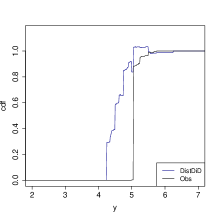
Figure A.2. Observed and Counterfactual Distributions: Top Quartile

Panel A. CS, Subgroup 1	Panel B. DistDiD, Subgroup 1
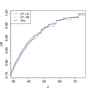
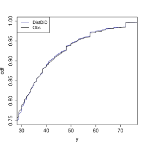
Panel C. CS, Subgroup 2	Panel D. DistDiD, Subgroup 2
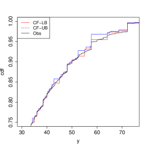
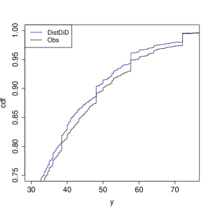
Notes: $Obs$ refers to $\hat{F}_{Y_{1}|D=1}$, $CF$-$LB$ ($CF$-$UB$) denotes the lower (upper) CS bound on $F_{Y_{10}|D=1}$, and $DistDiD$ refers to the distributional DiD estimate of $F_{Y_{10}|D=1}$. Subgroup 1 (Subgroup 2) refers to the subgroup of states with pre-treatment minimum wage $<\$8$ ($\geq\$8$).

Figure A.3. Observed Wage Distribution and CS Bounds on the Counterfactual Distribution

Panel A. Subgroup 1 (Pre-Treatment MW$<$$8	Panel B. Subgroup 2 (Pre-Treatment MW$\geq$$8)

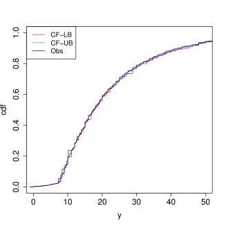
Figure A.4. Observed Wage Distribution and Distributional DiD Estimated Counterfactual Distribution

Panel A. Subgroup 1 (Pre-Treatment MW$<$$8)	Panel B. Subgroup 2 (Pre-Treatment MW$\geq$$8)

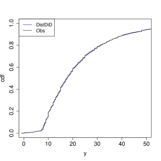
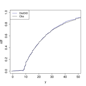
Appendix C Numerical Examples

In this section, we illustrate the wide applicability of the CS identification approach using several numerical examples of outcomes with discrete and mixed distributions. We consider four different marginal distributions presented in Table A.2, including the Poisson distribution (Example I), left- and right-censoring (Examples II-III) and a bunching example (Example IV). While Example I falls under the AI2006 identification results, the remaining examples are not covered by their approach.

Table A.2. Examples of Marginal Distributions of $Y_{t0}$

I. Poisson	$F_{Y_{t0}}(y)=\Pi_{t}(y)$, where $\Pi_{t}(\cdot)$ is the Poisson cdf with mean $\lambda_{t}$.
II. Left-censoring	$\left\{\text{\parbox{341.43306pt}{$F_{Y_{t0}}(y)=\left\{\begin{array}[]{ll}0&\text{if }y<c_{t}\\ \Lambda_{t}(y)&\text{if }y\geq c_{t}\end{array}\right.,$ \\ where $\Lambda_{t}(\cdot)$ is the $\chi^{2}$ cdf with $k_{t}$ degrees of freedom.}}\right.$
III. Right-censoring	$\left\{\text{\parbox{341.43306pt}{$F_{Y_{t0}}(y)=\left\{\begin{array}[]{ll}\Lambda_{t}(y)&\text{if }y<c_{t}\\ 1&\text{if }y\geq c_{t}\end{array}\right.$,\\ where $\Lambda_{t}(\cdot)$ is the $\chi^{2}$ cdf with $k_{t}$ degrees of freedom.}}\right.$
IV. Bunching	$\left\{\text{\parbox{341.43306pt}{$F_{Y_{t0}}(y)=\left\{\begin{array}[]{ll}\Phi_{t}(y)&\text{if }y\not\in[c_{t},w_{t})\\ \Phi_{t}(c_{t})+b_{t}(\Phi_{t}(w_{t})-\Phi_{t}(c_{t}))&\text{if }y=c_{t}\\ \Phi_{t}(c_{t})+b_{t}(\Phi_{t}(w_{t})-\Phi_{t}(c_{t}))+(1-b_{t})(\Phi_{t}(y)-\Phi_{t}(c))&\text{if }y\in(c_{t},w_{t})\end{array}\right.$\\ where $\Phi_{t}(.)$ is the standard normal cdf with mean $\mu_{t}$ and standard deviation $\sigma_{t}$.}}\right.$

Given marginal distributions of $Y_{00}$ and $Y_{10}$, we can generate conditional potential outcome distributions that satisfy the copula stability condition by the following, for $t=0,1$,

$$F_{Y_{t0}|D=0}(y) =\frac{1}{q}C_{Y_{0},D}(F_{Y_{t0}}(y),q),$$ (C.1)

$$F_{Y_{t0}|D=1}(y) =\frac{1}{p}\left(F_{Y_{t0}}(y)-C_{Y_{0},D}(F_{Y_{t0}}(y),q)\right).$$ (C.2)

We set $C_{Y_{0},D}(u,q)=(max(u^{-\theta}+q^{-\theta}-1,0))^{-1/\theta}$. In the following examples, we let $\theta=1$ to fulfil the strict monotonicity condition imposed on the horizontal copula for $u\in[0,1]$. Note that all parameters of the marginal distributions we consider are allowed to vary across time in an arbitrary manner.

Figures A.5-A.9 present the numerical examples. Each figure presents a plot of each of the observed distribution used in the evaluation of the CS bounds ($F_{Y_{0}|D=0}$, $F_{Y_{1}|D=0}$ and $F_{Y_{0}|D=1}$) in Panels A-C. Panel D of ech figure presents the counterfactual distribution for the treatment group ($F_{Y_{10}|D=1}$) together with the CS bounds labeled as $CF$ and $LB$/$UB$, respectively.

Figure A.5 illustrates our bounds for the Poisson example with $\lambda_{0}=1$ and $\lambda_{1}=3$. Since the CiC bounds proposed in AI2006 can be applied, we compute them and compare them to the CS bounds proposed here. In this numerical example, both bounding approaches coincide as illustrated in Panel D of Figure A.5.

Next, we examine mixed outcome distributions that fall outside the scope of the AI2006 identification results. Figures A.6-A.8 provide two different parametrizations of the left-censoring example (Example II). In the first case (Figure A.6), $RanF_{Y_{10}|D=1}\subset RanF_{Y_{0}|D=1}$ and, as a result, the counterfactual distribution is point-identified. In the second case (Figure A.8), $RanF_{Y_{10}|D=1}\not\subseteq RanF_{Y_{0}|D=1}$, and we therefore only attain partial identification of the counterfactual distribution. Figure A.8 illustrates the CS bounds for a right-censoring example (Example III), where the censoring cutoff as well as the degrees of freedom of the $\chi^{2}$ distribution vary across time. Finally, we consider a bunching example (Example IV), where the bunching cutoff ($c_{t}$), the width of the bunching window ($w_{t}-c_{t}$) and the bunching probability ($b_{t}$) are time-varying. One notable feature of the bunching example is that the potential outcome distributions are strictly increasing, but discontinuous. Panel D of Figure A.9 shows that the CS bounds in this bunching example cover the counterfactual distribution. Overall, for these mixed outcome distributions, our numerical analysis illustrates that point-identification of the counterfactual distribution is possible on the intersection of the range of $F_{Y_{10|D=1}}$ and $F_{Y_{0}|D=1}$, whereas only set-identification is possible outside this intersection.

Finally, it is important to discuss how the AI2006 CiC bounds would perform in the context of the mixed-outcome examples we consider. In several of these examples, the two quantiles used in the upper and lower bound in the AI2006 CiC bounds equal each other, specifically $Q_{Y_{0}|D=0}^{\mathbb{Y}_{0|0},+}(u)=Q_{Y_{0}|D=0}^{\mathbb{Y}_{0|0},-}(u)$ for $u\in(0,1)$ (e.g. Examples III and IV). It follows that the AI2006 CiC lower bound would equal its upper bound, and the CiC bounds would not include the counterfactual distribution. As AI2006 point out, the bound on quantiles that they exploit in their partial identification result for discrete outcomes is not valid for outcomes with mixed distributions.

Figure A.5. Numerical Example I: Poisson with $\lambda_{0}=1$, $\lambda_{1}=3$

Panel A. $F_{Y_{00}|D=0}$	Panel B. $F_{Y_{10}|D=0}$
Panel C. $F_{Y_{00}|D=1}$	Panel D. CS Bounds on $F_{Y_{10}|D=1}$
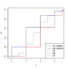
Notes: In Panel D, $CF$ denotes the counterfactual distribution for the treatment group ($F_{Y_{10}|D=1}$), $LB$-$AI2006$ ($UB$-$AI2006$) denotes the CiC lower (upper) bound from AI2006, and $LB$ ($UB$) denote the CS lower (upper) bound proposed here.

Figure A.6. Numerical Example II: Left-censoring, $c_{0}=c_{1}=5$, $k_{0}=5$, $k_{1}=3$

Panel A. $F_{Y_{00}|D=0}$	Panel B. $F_{Y_{10}|D=0}$
Panel C. $F_{Y_{00}|D=1}$	Panel D. CS Bounds on $F_{Y_{10}|D=1}$

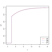
Figure A.7. Numerical Example II: Left-censoring, $c_{0}=c_{1}=5$, $k_{0}=3$, $k_{1}=5$

Panel A. $F_{Y_{00}|D=0}$	Panel B. $F_{Y_{10}|D=0}$
Panel C. $F_{Y_{00}|D=1}$	Panel D. CS Bounds on $F_{Y_{10}|D=1}$

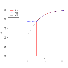
Figure A.8. Numerical Example III: Right-censoring, $c_{0}=5$, $c_{1}=10$, $k_{0}=3$, $k_{1}=5$

Panel A. $F_{Y_{00}|D=0}$	Panel B. $F_{Y_{10}|D=0}$
Panel C. $F_{Y_{00}|D=1}$	Panel D. CS Bounds on $F_{Y_{10}|D=1}$

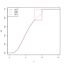
Figure A.9. Numerical Example IV: Outcome Distribution with Bunching

Panel A. $F_{Y_{00}|D=0}$	Panel B. $F_{Y_{10}|D=0}$
Panel C. $F_{Y_{00}|D=1}$	Panel D. CS Bounds on $F_{Y_{10}|D=1}$
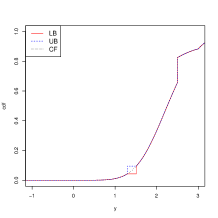
Notes: The figures are generated by numerically evaluating the conditional potential outcome distribution for the bunching example (IV) in Table A.2 with $c_{0}=0.5$, $w_{0}=1$, $c_{1}=2.5$, $w_{1}=3$, $b_{0}=0.25$, and $b_{1}=0.75$.

Appendix D Parallel Trends as Covariance Stability

Lemma A.4.

Suppose $\mathbb{P}(D=1)\in(0,1)$.

$$\mathbb{E}[Y_{10}-Y_{00}|D=1]=\mathbb{E}[Y_{10}-Y_{00}|D=0]~{}~{}\Longleftrightarrow~{}~{}Cov(Y_{00},D)=Cov(Y_{10,D}).$$

Proof.

The result follows by first multiplying $\mathbb{E}[Y_{10}-Y_{00}|D=1]-\mathbb{E}[Y_{10}-Y_{00}|D=0]$ by $\mathbb{P}(D=1)\mathbb{P}(D=0)$ and then simplifying the resulting expression as follows,

$$\mathbb{P}(D=1)\mathbb{P}(D=0)\mathbb{E}[Y_{10}-Y_{00}|D=1]-\mathbb{P}(D=1)\mathbb{P}(D=0)\mathbb{E}[Y_{10}-Y_{00}|D=0]$$

$$= \mathbb{P}(D=0)\mathbb{E}[(Y_{10}-Y_{00})D]-\mathbb{P}(D=1)\mathbb{E}[(Y_{10}-Y_{00})(1-D)]$$

$$= \mathbb{E}\left[(Y_{10}-Y_{00})(1-\mathbb{P}(D=1))D-(Y_{10}-Y_{00})(1-D)\mathbb{P}(D=1)\right]$$

$$= \mathbb{E}\left[(Y_{10}-Y_{00})(D-\mathbb{P}(D=1))\right]=\mathbb{E}\left[(Y_{10}-Y_{00})(D-\mathbb{E}[D])\right]$$

$$= Cov(Y_{10}-Y_{00},D).$$

The $\Longrightarrow$ ($\Longleftarrow$) direction follows from noting that it would imply the left-hand (right-hand) side of the equality is zero. ∎

Appendix E Conditional Time Invariance and Dependence Stability

In this section, we elaborate on the connection between the conditional time invariance condition in AI2006 and our copula stability condition.

The following result demonstrates that the AI2006 conditions for continuous, strictly increasing outcome distributions are equivalent to our copula stability assumption.

Claim D.1.

Assume the cdfs $F_{Y_{t0}}(.),t\in\{0,1\}$ are continuous and strictly increasing, then the two following statements are equivalent:

1. $C_{Y_{00},D}(u,q)=C_{Y_{10},D}(u,q)$ for all $u\in[0,1]$.

2. There exist two strictly increasing functions $h_{t}(.),t\in\{0,1\}$ and two uniformly distributed random variables over $[0,1]$ $U_{00}$ and $U_{10}$ such that $Y_{t0}=h_{t}(U_{t0})$ and $U_{00}|D=d\sim U_{10}|D=d$ for $d\in\{0,1\}$.

Proof.

(i) $\Longrightarrow$ (ii).

Since the cdf $F_{Y_{t0}}$ is continuous and strictly increasing, we have

$$Y_{t0} = Q^{\mathbb{R},-}_{Y_{t0}}\left(F_{Y_{t0}}(Y_{t0})\right),$$

$$= Q^{\mathbb{R},-}_{Y_{t0}}\left(U_{t0})\right),\ \text{ where }U_{t0}\equiv F_{Y_{t0}}(Y_{t0})\sim\mathcal{U}_{[0,1]},$$

$$= h_{t}(U_{t0}),\ \text{ where }h_{t}(u)\equiv Q^{\mathbb{R},-}_{Y_{t0}}(u).$$

By definition, $h_{t}$ is continuous and strictly increasing as is the quantile function $Q^{\mathbb{R},-}_{Y_{t0}}$. Then, the following equalities hold:

$$C_{Y_{t0},D} = C_{h_{t}(U_{t0}),D}=C_{U_{t0},D},$$

where the second equality holds from the invariance principle in Embrechts and Hofert (2013, Proposition 4(2)). Therefore,

$$C_{Y_{00},D}(u,q)=C_{Y_{10},D}(u,q) \Longrightarrow C_{U_{00},D}(u,q)=C_{U_{10},D}(u,q),$$

$$\Longrightarrow C_{U_{00},D}(F_{U_{00}}(u),F_{D}(0))=C_{U_{10},D}(F_{U_{10}}(u),F_{D}(0)),$$

$$\Longrightarrow F_{U_{00},D}(u,0)=F_{U_{10},D}(u,0),$$

$$\Longrightarrow u-F_{U_{00},D}(u,0)=u-F_{U_{10},D}(u,0),$$

$$\Longrightarrow F_{U_{00}}(u)-F_{U_{00},D}(u,0)=F_{U_{10}}(u)-F_{U_{10},D}(u,0),$$

$$\Longrightarrow \mathbb{P}(U_{00}\leq u,D=1)=\mathbb{P}(U_{10}\leq u,D=1),$$

where the second implication follows from $U_{t0}\sim\mathcal{U}_{[0,1]}$ and $F_{D}(0)=q$, the third holds from Sklar’s theorem, and the fifth follows from $U_{t0}\sim\mathcal{U}_{[0,1]}$. Hence, we have:

$$C_{Y_{00},D}(u,q)=C_{Y_{10},D}(u,q) \Longrightarrow \mathbb{P}(U_{10}\leq u,D=d)=\mathbb{P}(U_{10}\leq u,D=d)\text{ for }d\in\{0,1\},$$

$$\Longrightarrow \mathbb{P}(U_{00}\leq u,D=d)/\mathbb{P}(D=d)=\mathbb{P}(U_{10}\leq u,D=d)/\mathbb{P}(D=d),$$

$$\Longrightarrow F_{U_{00}|D}(u|d)\equiv\mathbb{P}(U_{00}\leq u|D=d)=\mathbb{P}(U_{10}\leq u|D=d)\equiv F_{U_{10}|D}(u|d),$$

$$\Longrightarrow U_{00}|D=d\sim U_{10}|D=d.$$

(ii) $\Longrightarrow$ (i). Suppose there exist two strictly increasing functions $h_{t}(.),t\in\{0,1\}$ and two uniformly distributed random variables over $[0,1]$ $U_{00}$ and $U_{10}$ such that $Y_{t0}=h_{t}(U_{t0})$ and $U_{00}|D=d\sim U_{10}|D=d$. Then, we have

$$F_{U_{00}|D}(u|d)=F_{U_{10}|D}(u|d) \Longrightarrow F_{U_{00}|D}(u|d)\mathbb{P}(D=d)=F_{U_{10}|D}(u|d)\mathbb{P}(D=d),$$

$$\Longrightarrow \mathbb{P}(U_{00}\leq u,D=d)=\mathbb{P}(U_{10}\leq u,D=d),$$

$$\Longrightarrow F_{U_{00},D}(u,0)=F_{U_{10},D}(u,0)\text{ for }d=0,$$

$$\Longrightarrow C_{U_{00},D}(F_{U_{00}}(u),F_{D}(0))=C_{U_{10},D}(F_{U_{10}}(u),F_{D}(0)),$$

$$\Longrightarrow C_{U_{00},D}(u,q)=C_{U_{10},D}(u,q),$$

$$\Longrightarrow C_{h_{0}(U_{00}),D}(u,q)=C_{U_{00},D}(u,q)=C_{U_{10},D}(u,q)=C_{h_{1}(U_{00}),D}(u,q),$$

$$\Longrightarrow C_{Y_{00},D}(u,q)=C_{Y_{10},D}(u,q),$$

where the fourth implication holds from Sklar’s theorem, the fifth follows from $U_{t0}\sim\mathcal{U}_{[0,1]}$, the sixth follows the invariance principle in Embrechts and Hofert (2013, Proposition 4.(2)), and the last holds from the assumption $Y_{t0}=h_{t}(U_{t0})$. ∎

While Claim D.1 shows that dependence stability is equivalent to the CiC assumptions with strict monotonicity and a continuous distribution of $U_{t}$, the following result (Claim D.2) shows that dependence stability and the general version of the CiC conditions with weak monotonicity are non-nested in general. An important caveat here is that to relate those two conditions we have to rely on a representation condition.

Before we proceed to Claim D.2, it is crucial to explain the reasoning behind the representation condition it requires. Specifically, that there exist $U_{t}\sim\mathcal{U}[0,1]$ for $t=0,1$, such that $(Y_{t0},D)\overset{d}{=}(Q_{Y_{t0}}^{-}(U_{t}),D)$ for $t=0,1$. The reasoning behind this representation condition stems from Proposition 2(2) in Embrechts and Hofert (2013), which implies that since $U_{t}\sim\mathcal{U}[0,1]$, $Q_{Y_{t0}}^{-}(U_{t})\sim F_{Y_{t0}}$. Since $Q_{Y_{t0}}^{-}$ is weakly monotonic by definition, Proposition 2(2) in Embrechts and Hofert (2013) therefore underscores that the weak monotonicity of the structural function as well as the scalar, continuous unobservable imposed in AI2006 holds wlog for any random variable. Proposition 2(2) in Embrechts and Hofert (2013) further implies that the time invariance of the marginal distribution of $U_{t}$ also holds wlog. Thus, it is the conditional time invariance restriction on $U_{t}|D$ that is the essential restriction in AI2006. Now note that since $U_{t}$ has a time-invariant continuous marginal distribution, the time invariance of the horizontal subcopula of $(U_{t},D)$ implies the conditional time invariance of the distribution of $U_{t}|D$ imposed in AI2006. As a result, in Claim D.2, we examine the relationship between dependence stablity of $(Y_{t0},D)$ and $(U_{t},D)$.

Part (i) of the following claim imposes dependence stability on $(Y_{t},D)$ and derives the implication on the relationship between the horizontal subcopulas of $(U_{t},D)$ for $t=0,1$. Part (ii) of the claim imposes dependence stability on $(U_{t},D)$ and derives the implication on the relationship between the horizontal subcopulas of $(Y_{t0},D)$ for $t=0,1$.

Claim D.2.

For $t=0,1$, consider $(Y_{t0},D)$ such that $Y_{t0}\sim F_{Y_{t0}}$ and $D$ is a binary variable with $\mathbb{P}(D=0)=q\in(0,1)$. Suppose that there exist $U_{t}\sim\mathcal{U}[0,1]$ for $t=0,1$ such that $(Y_{t0},D)\overset{d}{=}(Q_{Y_{t0}}^{-}(U_{t}),D)$ for $t=0,1$.

1. If $C_{Y_{00},D}(u,q)=C_{Y_{10},D}(u,q)$ for all $u\in[0,1]$, then for $v\in\overline{Ran}(F_{Y_{00}})\cap\overline{Ran}(F_{Y_{10}})$

   $$C_{U_{0},D}(v,q)=C_{U_{1},D}(v,q).$$ (E.1)

2. If $C_{U_{0},D}(v,q)=C_{U_{1},D}(v,q)$ for all $v\in[0,1]$, then for $u\in\overline{Ran}(F_{Y_{00}})\cap\overline{Ran}(F_{Y_{10}})$,

   $$C_{Y_{00},D}(u,q)=C_{Y_{10},D}(u,q).$$ (E.2)

Proof.

(i) For $y\in\mathbb{R}$

$$C_{Y_{t0},D}(F_{Y_{t}}(y),q)=F_{Y_{t0},D}(y,0)=\mathbb{P}(Y_{t0}\leq y,D=0)=\mathbb{P}(Q_{Y_{t0}}^{-}(U_{t})\leq y,D=0)$$

$$= \mathbb{P}(U_{t}\leq F_{Y_{t0}}(y),D=0)=C_{U_{t},D}(F_{Y_{t0}}(y),q).$$ (E.3)

where the first two equalities follow by definition. The third equality follows by the assumption that $(Y_{t},D)\overset{d}{=}(Q_{Y_{t0}}^{-}(U_{t}),D)$. The penultimate equality holds by Proposition 1(5) in Embrechts and Hofert (2013) and the right-continuity of $F_{Y_{t0}}$, which ensure that $Q_{Y_{t0}}^{-}(u)\leq y\Leftrightarrow u\leq F_{Y_{t0}}(y))$. As a result, for $t=0,1$, $C_{Y_{t0},D}(v,q)=C_{U_{t},D}(v,q)$ for $v\in\overline{Ran}(F_{Y_{t0}})$.

As a result, the dependence stability condition in Claim D.2(i), $C_{Y_{00},D}(u,q)=C_{Y_{10},D}(u,q)$ for all $u\in[0,1]$, implies the following for $v\in\overline{Ran}(F_{Y_{00}})\cap\overline{Ran}(F_{Y_{10}})$

$$C_{U_{0},D}(v,q)=C_{Y_{00},D}(v,q)=C_{Y_{10},D}(v,q)=C_{U_{1},q}(v,q)$$ (E.4)

where the first and last equalities follow from (E.3), whereas the second follows by the dependence stability assumption on $C_{Y_{t},D}$ imposed in Claim D.2(i).

(ii) For $y\in\mathbb{R}$,

$$F_{U_{t},D}(F_{Y_{t0}}(y),0)=C_{U_{t},D}(F_{Y_{t0}}(y),q)=\mathbb{P}(U_{t}\leq F_{Y_{t0}}(y),D=0)=\mathbb{P}(Q_{Y_{t0}}^{-}(U_{t})\leq y,D=0)$$

$$= \mathbb{P}(Y_{t0}\leq y,D=0)=C_{Y_{t0},D}(F_{Y_{t0}}(y),q)$$ (E.5)

where the first two equalities follow by definition, the third follows from Proposition 1(5) in Embrechts and Hofert (2013) since $F_{Y_{t0}}$ is increasing and right-continuous. The last two equalities follow by definition.

As a result, the dependence stablity condition imposed in Claim D.2(ii) implies the following for $u\in\overline{Ran}(F_{Y_{00}})\cap\overline{Ran}(F_{Y_{10}})$,

$$C_{Y_{00},D}(u,q)=C_{U_{0},D}(u,q)=C_{U_{1},D}(u,q)=C_{Y_{10},D}(u,q)$$ (E.6)

where the first and last equalities follow from (E.5), whereas the second follows by the dependence stability assumption on $C_{U_{t},D}$ imposed in Claim D.2(ii). ∎

Part (i) of Claim D.2 establishes that the copula stability on the potential outcomes implies copula stability for the unobservables for specific values on [0,1]. In general, this would not be sufficient for the conditional time invariance assumption in AI2006, except if $Ran(F_{Y_{00}})=Ran(F_{Y_{01}})=[0,1]$, that is, when outcomes are continuous. Part (ii) of Claim D.2 shows that copula stability on $(U_{t},D)$ implies the copula stability on $(Y_{t0},D)$ for $u\in[0,1]$ if $Ran(F_{Y_{00}})=Ran(F_{Y_{10}})=[0,1]$. However, in general, it would only hold on the intersection of the two ranges.

References

- (1)
- Aaberge, Havnes, and Mogstad (2013) Aaberge, R., T. Havnes, and M. Mogstad (2013): “A theory for ranking distribution functions,” Discussion Papers 763, Statistics Norway, Research Department.
- Abadie (2005) Abadie, A. (2005): “Semiparametric Difference-in-Differences Estimators,” The Review of Economic Studies, 72(1), 1–19.
- Almond, Hoynes, and Schanzenbach (2011) Almond, D., H. W. Hoynes, and D. W. Schanzenbach (2011): “Inside the War on Poverty: The Impact of Food Stamps on Birth Outcomes,” The Review of Economics and Statistics, 93(2), 387–403.
- Assunção, McMillan, Murphy, and Souza-Rodrigues (2022) Assunção, J., R. McMillan, J. Murphy, and E. Souza-Rodrigues (2022): “Optimal Environmental Targeting in the Amazon Rainforest,” The Review of Economic Studies.
- Athey and Imbens (2006) Athey, S., and G. W. Imbens (2006): “Identification and Inference in Nonlinear Difference-in-Differences Models,” Econometrica, 74(2), 431–497.
- Basri, Felix, Hanna, and Olken (2021) Basri, M. C., M. Felix, R. Hanna, and B. A. Olken (2021): “Tax Administration versus Tax Rates: Evidence from Corporate Taxation in Indonesia,” American Economic Review, 111(12), 3827–71.
- Berger, Herkenhoff, and Mongey (2022) Berger, D. W., K. F. Herkenhoff, and S. Mongey (2022): “Minimum Wages, Efficiency and Welfare,” Working Paper 29662, National Bureau of Economic Research.
- Blackorby and Donaldson (1978) Blackorby, C., and D. Donaldson (1978): “Measures of relative equality and their meaning in terms of social welfare,” Journal of Economic Theory, 18(1), 59–80.
- Boissel and Matray (2022) Boissel, C., and A. Matray (2022): “Dividend Taxes and the Allocation of Capital,” American Economic Review, 112(9), 2884–2920.
- Bonhomme and Sauder (2011) Bonhomme, S., and U. Sauder (2011): “Recovering Distributions in Difference-in-Differences Models: A Comparison of Selective and Comprehensive Schooling,” The Review of Economics and Statistics, 93(2), 479–494.
- Callaway and Li (2019) Callaway, B., and T. Li (2019): “Quantile treatment effects in difference in differences models with panel data,” Quantitative Economics, 10(4), 1579–1618.
- Card and Krueger (1994) Card, D., and A. B. Krueger (1994): “Minimum Wages and Employment: A Case Study of the Fast-Food Industry in New Jersey and Pennsylvania,” The American Economic Review, 84(4), 772–793.