BAA-NGP: Bundle-Adjusting Accelerated Neural Graphics Primitives

Abstract

Implicit neural representation has emerged as a powerful method for reconstructing 3D scenes from 2D images. Given a set of camera poses and associated images, the models can be trained to synthesize novel, unseen views. In order to expand the use cases for implicit neural representations, we need to incorporate camera pose estimation capabilities as part of the representation learning, as this is necessary for reconstructing scenes from real-world video sequences where cameras are generally not being tracked. Existing approaches like COLMAP and, most recently, bundle-adjusting neural radiance field methods often suffer from lengthy processing times. These delays ranging from hours to days, arise from laborious feature matching, hardware limitations, dense point sampling, and long training times required by a multi-layer perceptron structure with a large number of parameters. To address these challenges, we propose a framework called bundle-adjusting accelerated neural graphics primitives (BAA-NGP). Our approach leverages accelerated sampling and hash encoding to expedite both pose refinement/estimation and 3D scene reconstruction. Experimental results demonstrate that our method achieves a more than 10 to 20 $\times$ speed improvement in novel view synthesis compared to other bundle-adjusting neural radiance field methods without sacrificing the quality of pose estimation. The github repository can be found here https://github.com/IntelLabs/baa-ngp.

1 Introduction

Implicit neural representation (INR) has been widely used for novel view synthesis tasks in recent years. Given a set of known camera intrinsic and extrinsic parameters and a rough estimation of the boundary of the scene, we can learn an implicit 3D scene representation by sampling 3D points along camera rays and performing supervised learning against its ground-truth color [9]. The advantage of the INR is that when a novel view camera pose is queried within the bounded area, a novel view can be constructed at a wide range of resolutions.

One challenge with INR for novel view synthesis tasks is that current methods require accurate camera poses to be provided, which can be challenging to obtain, and also limits the applicability of many INR methods for poorly posed multi-view image sets or unposed video sequences. While popular methods like COLMAP [13, 14] have been used to estimate the camera poses from input images, they often miss frames and lead to suboptimal results. Optimization-based pose estimation and radiance field learning methods have been proposed to address this issue. Still, they can be computationally expensive, often take hours to be optimized on 100 images of size $400\times 400$ and unsuitable for real-time applications [7, 1].

Many recent works have focused on making INR learning faster. One such technique is named instant neural graphics primitives (iNGP) [11] that uses grid sampling and hash encodings to converge significantly faster (<5 seconds) than other techniques with ground truth poses. However, this approach has yet to consider datasets without camera poses or poorly estimated camera poses, which are more general and come from real-world data.

To address the current restrictions on knowing accurate camera poses a-priori as well as lengthy training time, we propose a novel approach called Bundle-Adjusting Accelerated Graphics Primitives (BAA-NGP) that can learn to estimate camera poses and optimize the radiance field simultaneously with 10 to 20 times speedup as is shown in Figure 1. This addresses the challenge of accelerated learning of INR models in unstructured settings without tracked cameras. BAA-NGP combines pose estimation with fast occupancy sampling and multiresolution hash encoding through a new curriculum learning strategy. We evaluate our proposed method on several benchmark datasets, including multi-view object-centric scenes as well as frontal-camera video sequences of unbounded scenes. We compare our results with state-of-the-art techniques such as BARF and COLMAP-based methods where camera poses are not known or are known imprecisely. Our results show that BAA-NGP achieves comparable or better performance to these state-of-the-art techniques while being significantly faster than the existing approaches, thereby widening its range of applicability to a broad set of real-world scenarios and applications ranging from virtual and augmented reality to robotics and automation.

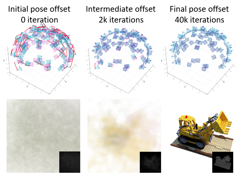
Figure 1: Starting from a state with inaccurate poses, BAA-NGP can optimize camera poses as well as learn an implicit representation within minutes of training.

2 Related Work

Despite the relatively recent development of INRs, an expansive number of approaches have been proposed in the literature. We focus the discussion therefore on works related to solving the problem of INRs that can learn without known camera poses.

Structure from motion (SfM) is a classical method often used for 3D structure reconstruction from 2D images or video sequences. It involves estimating the camera poses for each image and simultaneously recovering the 3D positions of the scene points, leveraging feature detection and matching across frames, and solving it all together via numerical optimization. The camera pose estimation techniques from SfM have been used in the context of INR training. COLMAP [13, 14] is a commonly used library for performing SfM, and many INR methods rely on this as part of their pipeline. However, COLMAP and other SfM techniques have high computational and memory requirements and rely heavily on the abundance of salient features in the scene, which may result in missing frames in scenes with limited or poor feature detection/saliency.

To avoid the limitations associated with using SfM for camera pose estimation, NeRF$--$ [18] and Self-Calibrating Neural Radiance Fields [5] learned camera pose estimates along with the neural radiance fields. These methods assumed forward-facing views and involved two-stage procedures for estimating camera poses and updating the neural radiance fields during training. Bundle-adjusting neural radiance field (BARF) [7] first proposed a direct end-to-end extrinsics estimation while learning the implicit 3D scene with NeRF. A coarse-to-fine feature weighting schedule for positional encoding features was used and was critical for smoothing the signals for pose updates. We improve their method and propose our coarse-to-fine weighting schedule best suited for learnable hash encoding features. Subsequent work with G-Nerf [8] used GANs to improve generalization to large baseline captures. Gaussian-Activated Radiance Fields [1] then proposed that without positional encoding, updating the activation function of the multi-layer perceptron can further improve the pose estimation and the quality of the results. However, a common thread among all these methods is that they still require an extensive amount of time (in the low tens of hours) to train.

To overcome the long training time of INR learning, recently, several methods have been proposed to accelerate the process from the aspect of sampling, encoding, and better hardware integration of the multilayer perceptron, including but not limited to [12, 3, 20, 19, 16]. However, these methods assume known camera poses. Methods that train on scenes without camera poses still rely on SfM, such as COLMAP, for pose estimation. Instead, a recent paper [4] presented a fast neural radiance field learning without a camera prior that avoided classical SfM methods. This work utilizes gradient smoothing and re-implemented iNGP in PyTorch in order to use multi-level learning rate scheduling to incorporate multi-resolution hash encoding with pose estimation. Unfortunately, the code is unavailable, so the performance cannot be cross-validated. Our work approaches the problem via a simple and novel coarse-to-fine feature re-weighting scheme and utilizes multi-resolution occupancy sampling, resulting in 10$\times$ shorter training iterations than this concurrent work. For unbounded scenes, we incorporate inverted sphere parameterization with hash encoding, which enables pose estimation for more general scenarios. Our codebase is available for comparison.

3 Methodology

3.1 Problem Formulation

Our goal is to learn INR models from images taken without known camera poses or poorly estimated poses. The INR model is described in general terms by a function

$$F_{\Theta}(p):\{x,y,z\}\rightarrow c,\sigma$$ (1)

where a 3D location in the scene $\{x,y,z\}$ maps to a 3-channel radiance color $c=\{r,g,b\}$ and density $\sigma\in[0,1]$. In order to reconstruct an image from a camera positioned and oriented as $p\in\mathbb{S}\mathbb{E}(3)$ in the scene, we apply a pixel-by-pixel ray marching procedure, where for each pixel location $[u,v]$, we integrate all the radiance values found along the ray going from the camera origin and passing through the pixel location $[u,v]$. Therefore, the output color of a pixel along the ray $R$ of a camera with pose $p$ can be defined as follows:

$$f(p,R)=\sum\nolimits_{i=1}^{N}\alpha_{i}T_{i}c_{i}$$ (2)

where $T_{i}=exp(-\sum_{j=1}^{i-1}\sigma_{j}\delta_{j})$ denotes the accumulated transmittance along the ray, and $c_{i}$ is the output color of sample $i$ from $F_{\Theta}(p)$, and $\alpha$ for each ray segment is calculated as

$$\alpha_{i}=1-exp(\sigma_{i}\delta_{i})$$ (3)

where $\delta_{i}$ is the distance between sample point $i$ and $i+1$. $\sigma_{i}$ is the density output of sample point $i$.

For training, given $M$ captured images $\{\mathcal{I}_{i}\}_{i=1}^{M}$ of width $W$ and height $H$ taken from the same scene, we learn the INR model while simultaneously, as a byproduct, learn the camera poses estimates $\{p_{i}\}_{i=1}^{M}\in\mathbb{R}^{6}$ associated with each image in $\{\mathcal{I}_{i}\}_{i=1}^{M}$.

Similar to [7, 1], we have no image order or sequence assumptions. We assume that camera intrinsics are known, but by definition, camera extrinsics are unknown. We also assume that the scene is static. Solving the problem involves minimizing the following loss function:

$$\min_{p_{1},...,p_{M},\Theta}\sum_{i=1}^{M}\sum_{j=1}^{W}\sum_{k=1}^{H}||\hat{\mathcal{I}}_{ijk}(p_{i},\Theta)-\mathcal{I}_{ijk}||_{2}^{2}$$ (4)

In this variation of the problem, the camera poses $\{p_{1}...p_{M}\}$ are optimization variables and are found jointly with the model parameters $\Theta$. Previous works investigating the problem of camera pose estimation have divided their attention across two domains that result in different datasets and objectives[7, 1]:

• Pose estimation (unbounded scene): Initialized from identity camera poses are reconstructed for a sequence of video with frames relatively close to each other, mostly covering “forward-facing scenes” as one would get from cellphone camera shots or mobile robots.

• Pose refinement (bounded scene): camera pose corrections are found for available but noisy camera poses for multi-viewpoint images of a centered object.

Small variations in the model are used to account for these two domains of data. Figure 2 shows the scenarios considered in this paper.

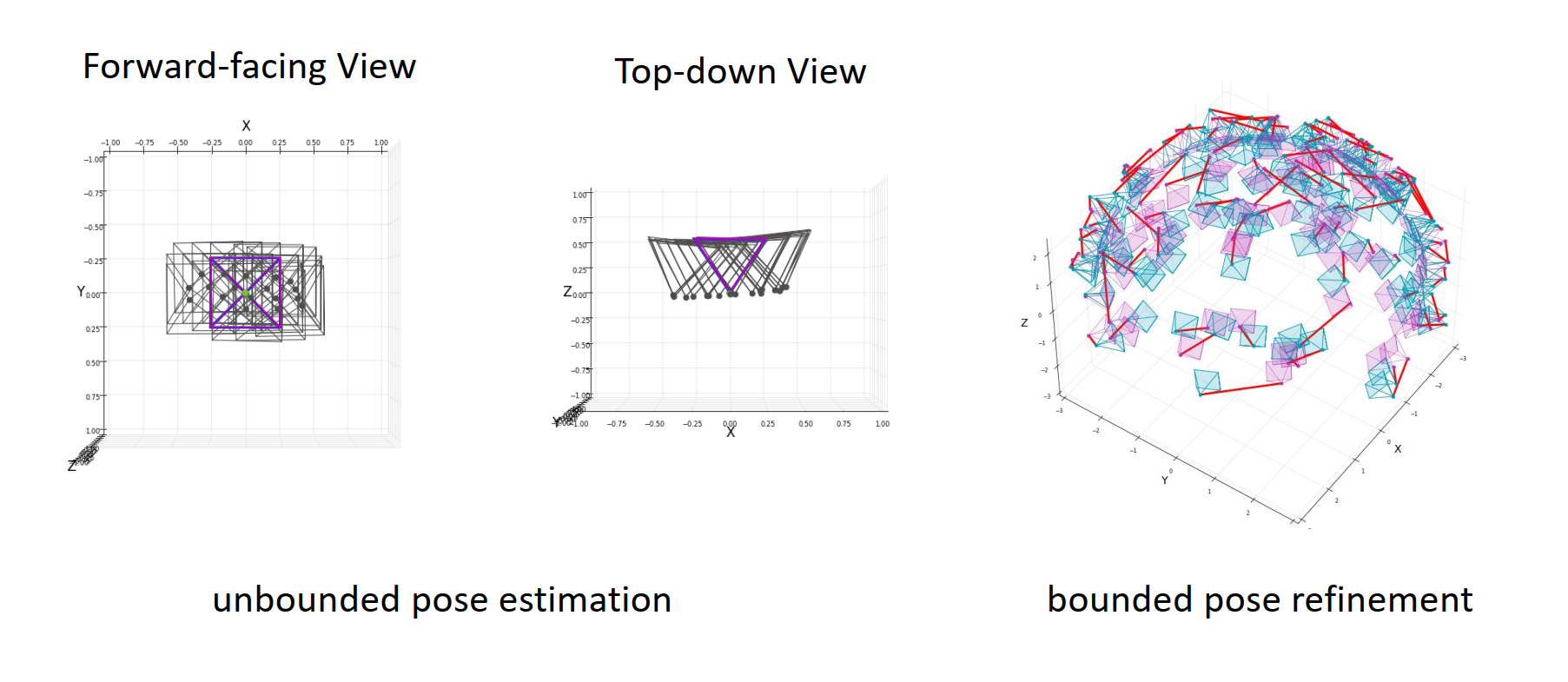
Figure 2: INRs use posed images from multiple viewpoints to reconstruct the scene. In our problem, we assume that a sequence of images was taken from unknown viewpoints for unbounded scenes (left) and poorly estimated viewpoints for bounded scenes (right). Purple frames are initial camera poses, gray/blue frames are ground truth camera poses, and the red line indicates a translation error.

3.2 Approach

3.2.1 Network Architecture

We start with an established model for learning implicit neural representations, i.e., neural radiance field, consisting of a neural network model for representing $F_{\theta}(p)$. One of the most successful models for this task is a multi-layered perceptron (MLP). Our final model involves the following stages for image reconstruction: inverted sphere parameterization, multi-resolution hash encoding, then a multi-layer perceptron decoder.

Parameterized camera poses to contracted/reparameterized 3D points: Since hash grids and occupancy grids need finite bounding boxes known in advance, handling bounded and unbounded scenes require different 3D space parameterizations. For bounded scenes with given bounding box, we use affine transformations to bring the volume of interest into axis-aligned bounding box $[0,1]^{3}$. For unbounded scenes, we apply an inverted sphere parameterization allowing compact mapping of close and far locations [21].

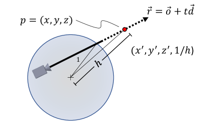
Figure 3: Reparameterization of 3D space via spherical contraction. Each point $p=(x,y,z)$ outside unit sphere is represented as a quadruple $(x^{\prime},y^{\prime},z^{\prime},1/h)$ that converts unbounded distances $h$ to bounded distances $1/h$.

In this case a point $(x,y,z)$ seen by a virtual camera with camera center $o\in\mathcal{R}^{3}$ along a ray $r=o+td$ with unit direction $d\in\mathcal{R}^{3}$, and with distance $t=[0,\infty]$, can be located arbitrarily far. To achieve bounded representation we use 2 different parameterizations based on the point location. A point within the unit sphere, centered at the origin, is unchanged. A point $(x,y,z)$, that is outside of the volume $h=\sqrt{x^{2}+y^{2}+z^{2}}>1$ is reparameterized by quadruple $(x^{\prime},y^{\prime},z^{\prime},1/h)$, where $(x^{\prime},y^{\prime},z^{\prime})=(x,y,z)/h$, and $x^{\prime 2}+y^{\prime 2}+z^{\prime 2}=1$. Then affine transformations are used to bring points within the volume into $[0,1]^{3}$ and reparameterized 4D representation into $[0,1]^{4}$.

Multiresolution Hash Encoding: We use multi-resolution hash encoding [11] to speed up the radiance field learning. Multi-resolution hash encoding transforms every input 3D point into a higher dimension concatenated features learned from each resolution level. For each point, $x\in\mathbb{R}^{d}$, the method first finds the grid cell in which the point resides, then $d$-linearly interpolates the features at vertices of the grid cell to produce an F-dimensional feature vector for the point $x$. Features from multiple resolution levels are then concatenated into a single vector. Instead of explicitly storing vertex features in a regular grid of size $N$ along each dimension, which would result in $N^{d}$ features for a level, hash encoding fixes the total number of F-dimensional features per level to be T. Hence if a coarser level needs less than $T$ features, the mapping remains 1:1, but if a finer level requires more than $T$ features, a spatial hash function (eq. 5) [17] is then used to map them into $T$ sets of features.

$$h(x)=(\bigoplus_{i=1}^{d}x_{i}\pi_{i})\ mod\ T$$ (5)

where $x$ denotes the vertex position in d dimension, $\bigoplus$ indicates the bitwise XOR, and $\pi_{1}=1,\pi_{2}=2654435761,\pi_{3}=805459861$ are selected by the original authors [11].

By specifying the base resolution ($N_{min}$) and the maximum resolution ($N_{max}$) of the grid, for $L$ levels, the grid resolution in between is chosen by $N_{l}=\lfloor N_{min}\cdot b^{l}\rfloor$, where b is calculated based on Equation 6.

$$b=exp((lnN_{max}-lnN_{min})/(L-1))$$ (6)

A value along a dimension of a point within the range of 0 and 1 can be mapped to a certain grid cell along that dimension within the $l$ layers via $\lfloor{x_{l}}\rfloor$ and $\lceil{x_{l}}\rceil$, where $x_{l}=x\cdot N_{l}$. The $d$-linear interpolation weight for that dimension can then be found, for example, via $w_{l}=x_{l}-\lfloor x_{l}\rfloor$ for that vertex corner.

Multi-layer Perceptron: Multiplayer perceptrons are commonly used for capturing neural radiance fields. Here we incorporate fully fused implementation of MLPs[11] with one layer for density learning and two layers for color learning which takes the output of the density layer as well as the view directions. The MLPs take in the encoded learnable features from multi-resolution hash encoding concatenated with direction encoded with spherical harmonics transform and output color and density for each corresponding 3D query point.

3.3 Training Strategies

Occupancy Grid Sampling

For further acceleration, we adopted coarse multiscale grid sampling before passing points through the radiance field for gradient backpropagation. Our occupancy grid is defined around the origin with an axis-aligned bounding box. The density of the sampled points is first queried without gradient to check if they hit free space. Only points that reside in a coarse grid cell that do not return free space (above a certain threshold) will be passed through for backpropagation.

Signal Coarse-to-Fine Smoothing

A vanilla coarse-to-fine smoothing technique had previously been proposed [7] that shields the earlier stage of the pose estimation from being affected by high-frequency information and slowly introduces such information at later stages for better pose fine-tuning and better image reconstruction quality. They use positional encoding and weigh the $k$-th frequency components of the inputs with $w_{k}$:

$$w_{k}(\alpha)=\begin{cases}0&\text{if}\alpha<k\\ \frac{1-cos((\alpha-k)\pi)}{2}&\text{if}\ 0\leq\alpha-k<1\\ 1&\text{if}\ \alpha-k\geq 1\\ \end{cases}\\$$ (7)

where $\alpha_{i}=\frac{s_{i}-r_{s}}{r_{e}-r_{s}}$, $r_{s}$ indicates the coarse-to-fine starting point as the percentage of the training progress, $r_{e}$ indicates the coarse-to-fine ending point as the percentage of the training progress. $s$ indicates the percentage of training progress so far at step $i$. This method assumes the original coordinates are concatenated with the positional encoding features and allows initial pose estimation learning with just 3D points as inputs.

We propose a novel coarse-to-fine strategy better suited for learnable hash encoding features. Since hash grid features, accompanying the very small MLP, carry information about density and radiance distributions in the volume, they are not equivalent to scene-agnostic frequency encoding of the 3D coordinates. Using 0 weights of the cosine window to nullify the features at finer levels results in MLP getting stuck at the early local minima and failing to learn hash grid features efficiently. Instead, starting with the coarsest level enabled, we prime the MLP by using coarse-level features in lieu of windowed-out fine-level features. We gradually replace such coarse-level estimates with the actually learned fine-level values as the cosine window expands. Therefore the features are weighted as follows

$$\gamma_{k}(x;\alpha)=w_{k}(\alpha)\cdot d_{k}+(1-w_{k}(\alpha))\cdot d_{\alpha}$$ (8)

where $d_{\alpha}$ indicates the set of features that has the highest grid level with a nonzero weight.

4 Experiments

4.1 Dataset

In order to evaluate BAA-NGP, we benchmarked our methods on the LLFF dataset for frontal-camera in-the-wild video sequences and the blender synthetic dataset for pose refinement. The following describes the dataset and the associated model architectures:

LLFF

We benchmark our methods for frontal camera pose estimation of the LLFF dataset. This video sequence dataset has images from continuous camera poses that concentrate the views at one side of the scene. The challenge of this dataset is that not many frames of each video sequence are available, and all cameras are posed on one side of the scene, giving limited coverage from multiple viewpoints. For our experiments, we resized images to $640\times 480$ for training and evaluation.

For the network training setup, we use occupancy sampling, inverted sphere reparameterization for input points, and two sets of multiresolution hash encoding for in-sphere and outside spaces in addition to the vanilla MLP setup. Similar to [7], all cameras are initialized with the identity transformation. We use the Adam optimizer and train the models for each scene with 20K iterations. The number of randomly sampled pixel rays is initialized as 1024 and dynamically adjusted throughout the training to keep the total number of samples taken along the rays consistent. The learning rate of the network is initialized as $1\times 10^{-4}$ and linearly increased to $1\times 10^{-2}$ for the first 100 iterations, and then step decayed by a factor of 0.33 at 10000, 15000, and 18000 iterations. Following a similar pattern, the learning rate of the camera poses is initialized as $3\times 10^{-4}$ and linearly increased to $3\times 10^{-3}$ for the first 100 iterations, and then step decayed by a factor of 0.33 at 10000, 15000, and 18000 iterations.

Blender synthetic

We evaluated our methods using the Blender synthetic dataset, which includes imperfect camera pose estimations, for camera pose refinement and scene reconstruction. This dataset comprises 100 training and 200 testing images, which we resized to $400\times 400$ for training and evaluation. The multi-view image sets, captured from the upper hemisphere of the central object, are rendered against a white background.

In terms of network training setup, we incorporated occupancy sampling, multiresolution hash encoding ($N_{min}=14$, $N_{max}=4069$, $L=16$), and signal coarse-to-fine smoothing ($r_{s}=0.1$, $r_{e}=0.5$), with the vanilla MLP setup. The camera poses were perturbed by adding noise $\mathcal{N}(0,0.15\mathbf{I})$ to the ground-truth poses, similar to the setup in Lin et al. [7]. We trained the model for each scene over 40K iterations. We used the Adam optimizer and applied an exponentially decaying learning rate schedule, starting from $1\times 10^{-2}$ and decaying to $1\times 10^{-4}$ for the network, and $1\times 10^{-3}$ decaying to $1\times 10^{-5}$ for the camera poses.

4.2 Metrics

We benchmarked our experiments for both novel view image reconstruction quality and pose estimation accuracy. For novel view synthesis, peak signal-to-noise ratio (PSNR), structural similarity index (SSIM) [22], multi-scale structural similarity index (MS-SSIM). Learned perceptual image patch similarity (LPIPS) [22] are used to evaluate the predicted image quality against the ground truth novel views. For pose estimation, we evaluate the camera pose rotation and translation differences between the predicted and the ground truth camera set after using Procrustes analysis for alignment. Please refer to supplementary information for details.

4.3 Results

Unposed Frontal Camera Video Sequences

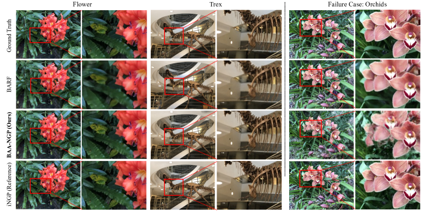
Figure 6: Qualitative analysis of BAA-NGP on the LLFF dataset. We show that our results are on par with BARF’s results but converge 20 $\times$ faster.

Figure 6 shows sample results of BAA-NGP on the frontal camera video sequences from LLFF, demonstrating qualitatively the high amount of detail in the reconstructed images. The last column of Figure 6 shows the only case (orchids) where our method fails to converge. It could be partially explained by the suboptimal performance of iNGP in this data, as shown in Table 2. Quantitatively, Table 2 shows our benchmarking data against the state-of-the-art algorithms. We show that BAA-NGP can achieve more than $20\times$ speedup with similar quality as BARF, whereas our metrics are better or on par for almost all metrics except rotation. Qualitatively, our method captures more details as observed in the reconstructed images.

Imperfect Poses Refinement for Multi-View Synthetic Images

Figure 5 shows the results of imperfect pose refinement for multi-view synthetic images. Qualitatively, BAA-NGP produces better-quality image synthesis with cleaner backgrounds and finer details. For quantitative analysis, as shown in Table 1, the results demonstrate that BAA-NPG not only yields similar pose estimation results and improved image synthesis quality but also achieves a more than 10-fold speedup. One observation from this result is that the Materials scenes in the dataset were more challenging, likely due to the limitations of hash grid feature encoding. The authors of iNGP reported similar findings when using ground truth camera poses, attributing this issue to the dataset’s high complexity and view-dependent reflections [11].

Homography Recovery

We also conducted a homography recovery experiment as an analogy to 3D cases to evaluate the effectiveness of homography matrix estimation using multi-resolution hash encoding architecture combined with multi-layer perception. We can consider equation 4 as a general case for homography recovery if we define $p_{i}$ as the parameterized warp transformation. We used the same setup as bundle-adjusting neural radiance field [7], where five warped patches are used for training as is shown in Figure 4(left). 2D multi-resolution hash encoding and fully fused multi-layer perceptrons were used as the main network architecture, and coarse-to-fine feature weighting was used for the best performance. For this experiment, $N_{min}=3,L=18$, coarse-to-fine $r_{s}=0.1,r_{e}=0.5$, learning rate for features and parameters was $1.e-2$ and for warp parameters was $3.e-3$. Adam optimizer was used for both learning processes, and training was conducted over 5000 epochs.

We show in Figure 4(right) that without signal coarse-to-fine smoothing, the learned features of hash encoding converge without learning any warping functions, which end up learning the most-overlapped area. With vanilla coarse-to-fine masking, pose estimation can be trapped in local minimal. With our coarse-to-fine implementation, we can achieve better pose estimation.

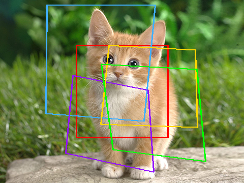
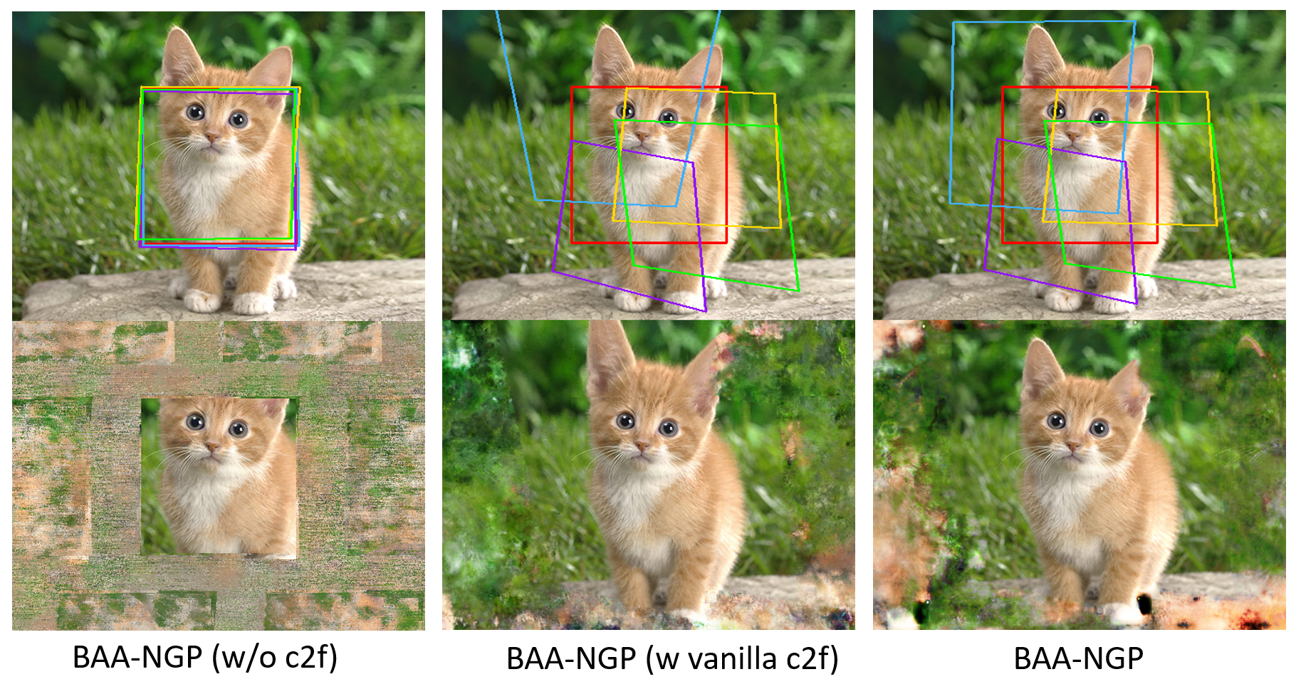
Figure 4: Experiment of tomography recovery on the cat image. (left) We used five different colors to show five different ground truth warped patches. (right) Results of different coarse-to-fine weighting procedures. We observe that our coarse-to-fine weighting scheme outperforms the vanilla coarse-to-fine weighting scheme qualitatively for both 2D tomography recovery and 3D pose refinement.

Table 1: Quantitative evaluation of pose refinement for the blender synthetic dataset. We show that our results are on par with BARF[7] in terms of camera pose estimation, with 10x faster training time, we achieve better visual synthesis quality overall.

Scene Camera pose registration Visual synthesis quality Training Time Rotation(°) $\downarrow$ Translation $\downarrow$ PSNR $\uparrow$ SSIM $\uparrow$ MS-SSIM $\uparrow$ LPIPS $\downarrow$ BARF ours BARF ours BARF ours BARF ours BARF ours BARF ours BARF ours Chair 0.093 0.093 0.405 0.658 31.15 34.36 0.952 0.985 0.990 0.996 0.074 0.026 04:26:30 00:30:09 Drums 0.046 0.029 0.202 0.134 23.91 25.03 0.895 0.934 0.954 0.971 0.147 0.072 04:28:06 00:26:10 Ficus 0.080 0.032 0.464 0.161 26.26 30.27 0.930 0.979 0.975 0.991 0.109 0.026 04:21:56 00:25:34 Hotdog 0.229 0.088 1.165 0.529 34.59 37.00 0.969 0.982 0.992 0.994 0.059 0.029 04:24:52 00:26:38 Lego 0.081 0.040 0.330 0.144 28.31 32.20 0.924 0.975 0.981 0.993 0.106 0.025 04:24:21 00:26:12 Materials 0.837 1.021 2.703 4.944 27.85 27.16 0.934 0.943 0.984 0.983 0.107 0.077 04:23:13 00:23:46 Mic 0.065 0.046 0.277 0.260 31.00 34.28 0.966 0.987 0.992 0.995 0.065 0.018 04:22:25 00:32:46 Ship 0.086 0.061 0.341 0.318 27.49 29.71 0.841 0.864 0.938 0.939 0.196 0.123 04:25:59 00:23:31 Mean 0.190 0.176 0.736 0.894 28.82 32.50 0.926 0.953 0.976 0.983 0.108 0.050 04:24:40 00:26:51

Table 2: Quantitative evaluation of pose estimation for the LLFF dataset. We show that our results are comparable to BARF with much less training time. iNGP[11] results are included for reference.

Scene Camera pose registration Visual synthesis quality Training Time Rotation(°) $\downarrow$ Translation $\downarrow$ PSNR $\uparrow$ SSIM $\uparrow$ MS-SSIM $\uparrow$ LPIPS $\downarrow$ [7] ours [7] ours [7] ours iNGP[11] [7] ours iNGP[11] [7] ours iNGP[11] [7] ours iNGP[11] [7] ours iNGP[11] Fern 0.163 3.978 0.188 1.733 23.96 19.02 25.42 0.709 0.504 0.822 0.916 0.717 0.948 0.390 0.480 0.182 05:23:29 0:10:45 0:07:33 Flower 0.224 2.258 0.233 0.530 24.07 25.52 26.78 0.712 0.811 0.851 0.891 0.935 0.952 0.379 0.157 0.139 05:24:55 0:10:39 0:08:21 Fortress 0.460 0.786 0.352 0.733 28.86 28.59 28.54 0.816 0.825 0.882 0.950 0.946 0.967 0.266 0.203 0.113 05:44:05 0:11:16 0:08:16 Horns 0.135 1.042 0.162 0.643 23.12 19.57 20.47 0.734 0.724 0.755 0.915 0.879 0.845 0.423 0.307 0.262 05:22:02 0:18:54 0:07:32 Leaves 1.274 1.249 0.253 0.342 18.67 20.14 20.80 0.529 0.687 0.738 0.831 0.902 0.922 0.474 0.264 0.243 06:47:43 0:18:37 0:08:07 Orchids 0.629 6.110 0.409 2.956 19.37 12.28 19.60 0.570 0.143 0.682 0.853 0.243 0.888 0.423 0.608 0.220 05:14:03 0:10:3 0:07:26 Rooms 0.362 1.853 0.293 1.856 31.60 29.15 34.03 0.937 0.900 0.969 0.981 0.963 0.986 0.230 0.271 0.095 05:35:49 0:20:23 0:07:55 T-rex 1.030 1.749 0.641 1.005 22.32 23.41 25.18 0.771 0.861 0.892 0.927 0.950 0.960 0.355 0.185 0.121 05:10:04 0:10:37 0:07:37 Mean 0.535 2.378 0.316 1.225 24.00 22.21 25.10 0.722 0.682 0.824 0.908 0.817 0.934 0.369 0.309 0.172 05:35:16 0:13:54 0:08:53

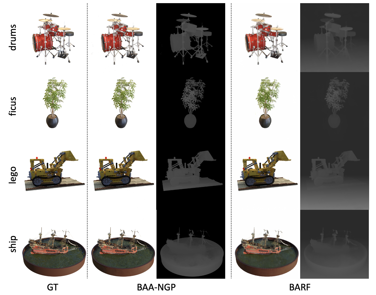
Figure 5: Qualitative analysis of BAA-NGP on the blender synthetic dataset. BAA-NGP produces better quality in image synthesis with cleaner backgrounds and finer details than BARF with 10 $\times$ less time.

5 Conclusion

In conclusion, we presented a method for learning INRs of scenes with unknown or poorly known camera poses while achieving learning rates in minutes. BAA-NGP, therefore, is a solution for addressing accelerated learning of INR models in unstructured settings. Our evaluations over several benchmark datasets, including multi-view object-centric scenes as well as frontal-camera video sequences of unbounded scenes, show that it is either comparable or outperforms state-of-the-art techniques such as BARF and COLMAP-based methods where camera poses are not known or are known imprecisely, and where training would otherwise take hours. Thus, this approach opens learning INRs for a broad set of real-world scenarios and applications ranging from virtual and augmented reality to robotics and automation, where time and unstructured image capture is vital.

One observation is that when our rendering baseline iNGP leads to suboptimal results, the corresponding results of BAA-NGP will also be influenced. In the future, we plan to improve iNGP with smarter ray sampling and 3D point contraction methods, which we found affected the performance of iNGP on unbounded scenes like LLFF data.

Supplementary

Implementation Details

We use one NVIDIA RTX3090 GPU, and build our architecture on top of nerfacc[6] code base, which utilizes pytorch, and contains CUDA acceleration. We use hash encoding API from tiny-cuda-nn [10].

Results Details

In Table 3 we show that with 20k iterations instead of 40k mentioned in the paper, our model can achieve similar performance with BARF[7] on the blender synthetic dataset. BARF runs around 200 to 300ms per iteration, whereas BAA-NGP runs around 100 to 150ms per iteration. Utilizing occupancy sampling adds some overhead per iteration compared to the basic BAA-NGP setup, hash grid encoding with simple MLPs, but it results in faster convergence throughout the training process.

Metrics Details

We benchmark our experiments for both novel view image reconstruction quality as well as pose estimation accuracy. For novel view synthesis, peak signal-to-noise ratio (PSNR), structural similarity index (SSIM) [22], multi-scale structural similarity index (MS-SSIM), learned perceptual image patch similarity (LPIPS) [22] are used to evaluate the predicted image quality against the ground truth novel views. For pose estimation, we evaluate the camera pose rotation and translation differences between the predicted camera set and the ground truth camera set after using procrustes analysis for alignment.

PSNR$\uparrow$

provides a comparison between the ground truth novel image and the reconstructed image queried from the same novel view camera position. Formally, PSNR is formulated as shown in eq. 9. This equation is expressed as the log ratio between the maximum possible value of a signal ($MAX=255$ for 8-bit image pixel) and the power of distorting noise ( pixel-wise mean squared error over all color channels, eq. 10) that affects the quality of the image reconstruction ($\hat{\mathcal{I}}$). A higher PSNR value in decibels (dB) suggests the image is closer to the ground truth image ($\mathcal{I}$), which indicates better fidelity.

$$PSNR(\mathcal{I},\hat{\mathcal{I}})=10\cdot log_{10}\frac{MAX^{2}}{\sqrt{MSE(\mathcal{I},\hat{\mathcal{I}})}}$$ (9)

$$MSE(\mathcal{I},\hat{\mathcal{I}})=\frac{1}{\sqrt{mn}}\cdot\sum_{i=0}^{m-1}\sum_{j=0}^{n-1}||\mathcal{I}_{ij}-\hat{\mathcal{I}}_{i,j}||^{2}$$ (10)

We follow the convention and report the simplified version of equation 9 using equation 11.

$$PSNR(\mathcal{I},\hat{\mathcal{I}})=-10\cdot log_{10}(MSE(\mathcal{I},\hat{\mathcal{I}}))$$ (11)

SSIM$\uparrow$

evaluates the structure similarity between images by considering luminance, contrast, and structural components. The value is between -1 and 1, where 1 indicates perfect similarity. Unlike PSNR, SSIM considers perceptual aspects, hence is more correlated with human perception. The formulation is shown in eq 12 [2]

$$SSIM(\mathcal{I},\hat{\mathcal{I}})=[l(\mathcal{I},\hat{\mathcal{I}})]^{\alpha}\cdot[c(\mathcal{I},\hat{\mathcal{I}})]^{\beta}\cdot[s(\mathcal{I},\hat{\mathcal{I}})]^{\gamma}$$ (12)

where $l(\mathcal{I},\hat{\mathcal{I}})=\frac{2\mu_{\mathcal{I}}\cdot\mu_{\hat{\mathcal{I}}}+C_{1}}{\mu_{\mathcal{I}}^{2}+\mu_{\hat{\mathcal{I}}}^{2}+C_{1}}$ is for luminance comparison, $c(\mathcal{I},\hat{\mathcal{I}})=\frac{2\sigma_{\mathcal{I}}\cdot\sigma_{\hat{\mathcal{I}}}+C_{2}}{\sigma_{\mathcal{I}}^{2}+\sigma_{\hat{\mathcal{I}}}^{2}+C_{2}}$ is for contract comparison, and $s(\mathcal{I},\hat{\mathcal{I}})=\frac{\sigma_{\mathcal{I}\hat{\mathcal{I}}}+C_{3}}{\sigma_{\mathcal{I}}^{2}+\sigma_{\hat{\mathcal{I}}}^{2}+C_{3}}$ is for structure comparison. $\mu$ and $\sigma$ are the average and standard deviations of the pixel intensities for each image, and $\sigma_{I\hat{I}}$ indicates the covariance of the pixel intensities between the two images. $C$ indicates a constant that is used to stabilize the division with weak denominators, and $\alpha,\beta,\gamma$ can be used to adjust the importance given to each component. For simplicity, we use the following equation from [2]

$$SSIM(\mathcal{I},\hat{\mathcal{I}})=\frac{(2\mu_{\mathcal{I}}\cdot\mu_{\hat{\mathcal{I}}}+C_{1})\cdot(2\sigma_{\mathcal{I}\hat{\mathcal{I}}}+C_{2})}{(\mu_{\mathcal{I}}^{2}+\mu_{\hat{\mathcal{I}}}^{2}+C_{1})\cdot(\sigma_{\mathcal{I}}^{2}+\sigma_{\hat{\mathcal{I}}}^{2}+C_{2})}$$ (13)

where $C_{1},C_{2}$ here are defined in eq. 14

$$C_{i}=(K_{i}\cdot MAX)^{2}$$ (14)

where $K_{1}=0.01,K_{2}=0.03$ are chosen by the original authors[22].

MS-SSIM$\uparrow$

is a multi-scale SSIM approach that considers structural similarity at different scales, which can capture more complex visual information, hence more robust to variations in scale and structure. The value is between 0 and 1. The formulation is as follows

$$MS-SSIM(\mathcal{I},\hat{\mathcal{I}})=[l(\mathcal{I},\hat{\mathcal{I}})]^{\alpha^{M}}\prod_{j=1}^{M}\cdot[c(\mathcal{I},\hat{\mathcal{I}})]^{\beta^{j}}\cdot[s(\mathcal{I},\hat{\mathcal{I}})]^{\gamma^{j}}$$ (15)

$M$ here indicates the number of decomposition levels. Similar simplification is utilized for SSIM calculation [2].

LPIPS$\downarrow$

uses deep neural networks to assess the high-level visual perceptual similarity between images. Image patch similarities are measured based on extracted learned features. The score also ranges 0 and 1, whereas lower score indicates higher similarity. The equation is as follows

$$LPIPS(\mathcal{I},\hat{\mathcal{I}})=\sum_{l=1}^{L}\frac{1}{H_{l}W_{l}}\sum_{h=1,w=1}^{H_{l},W_{l}}||w_{l}\odot(\hat{y}_{\mathcal{I}_{hw}}^{l}-\hat{y}_{{\hat{\mathcal{I}}}_{hw}}^{l})||_{2}^{2}$$ (16)

where $L$ is the total number of extracted feature layers. $H_{l}$ and $W_{l}$ are the height and width of features extracted from the $l$’s layer. $\hat{y_{\mathcal{I}}},\hat{y}_{\hat{\mathcal{I}}}\in\mathbb{R}^{H_{l}\times W_{l}\times C_{l}}$ denotes the features unit-normalized in the channel dimension for $I$ and $\hat{I}$. $\odot$ indicates channel-wise multiplication. We use pretrained VGG[15] network as the feature extraction backbone.

Rotation and Translation Error$\downarrow$

Rotation and translation errors for aligned ground truth camera poses and the estimated camera poses are evaluated based on the following equations

$$R_{error}(P,Q)=arccos\frac{tr(PQ^{*})-1}{2}$$ (17)

The rotation error $R_{error}$is defined as the distance (angle) between the rotations $P$ and $Q$. $PQ^{*}$ gives the distance rotation matrix.

Table 3: Quantitative evaluation of pose refinement for the blender synthetic dataset. We show that our results are on par with BARF[7] in terms of camera pose estimation, with much less time for training, we achieve similar visual synthesis quality overall. Time variations may be due to limitations of computing resources at the time of submission. The results we used for barf are reproduced by running their original code.

Scene Camera pose registration Visual synthesis quality Training Time Rotation(°) $\downarrow$ Translation $\downarrow$ PSNR $\uparrow$ SSIM $\uparrow$ MS-SSIM $\uparrow$ LPIPS $\downarrow$ BARF ours BARF ours BARF ours BARF ours BARF ours BARF ours BARF ours Chair 0.093 0.077 0.405 0.440 31.15 36.00 0.952 0.985 0.990 0.997 0.074 0.02 04:26:30 00:17:21 Drums 0.046 0.048 0.202 0.202 23.91 25.90 0.895 0.932 0.954 0.968 0.147 0.08 04:28:06 00:16:03 Ficus 0.080 0.056 0.464 0.223 26.26 31.24 0.930 0.978 0.975 0.991 0.109 0.03 04:21:56 00:15:06 Hotdog 0.229 0.105 1.165 0.519 34.59 37.04 0.969 0.982 0.992 0.994 0.059 0.03 04:24:52 00:16:05 Lego 0.081 0.055 0.330 0.166 28.31 33.52 0.924 0.976 0.981 0.993 0.106 0.02 04:24:21 00:07:41 Materials 0.837 1.111 2.703 18.538 27.85 22.42 0.934 0.873 0.984 0.942 0.107 0.09 04:23:13 00:15:52 Mic 0.065 0.059 0.059 0.293 31.00 35.07 0.966 0.987 0.992 0.995 0.065 0.02 04:22:25 00:18:15 Ship 0.086 1.004 0.341 4.572 27.49 29.33 0.841 0.882 0.938 0.949 0.196 0.13 04:25:59 00:14:19 Mean 0.190 0.314 0.736 3.119 28.82 31.32 0.926 0.949 0.976 0.979 0.108 0.053 04:24:40 00:15:20

References

- [1] Shin-Fang Chng, Sameera Ramasinghe, Jamie Sherrah, and Simon Lucey. Garf: Gaussian activated radiance fields for high fidelity reconstruction and pose estimation. Arxiv, 2016.
- [2] Gongfan Fang. Pytorch ms-ssim. https:https://github.com/VainF/pytorch-msssim, 2019.
- [3] Jiemin Fang, Lingxi Xie, Xinggang Wang, Xiaopeng Zhang, Wenyu Liu, and Qi Tian. Neusample: Neural sample field for efficient view synthesis. arXiv preprint arXiv:2111.15552, 2021.
- [4] Hwan Heo, Taekyung Kim, Jiyoung Lee, Jaewon Lee, Soohyun Kim, Hyunwoo J. Kim, and Jin-Hwa Kim. Robust camera pose refinement for multi-resolution hash encoding. Arxiv, 2023.
- [5] Yoonwoo Jeong, Seokjun Ahn, Christopher Choy, Anima Anandkumar, Minsu Cho, and Jaesik Park. Self-calibrating neural radiance fields. In Proceedings of the IEEE/CVF International Conference on Computer Vision, pages 5846–5854, 2021.
- [6] Ruilong Li, Hang Gao, Matthew Tancik, and Angjoo Kanazawa. Nerfacc: Efficient sampling accelerates nerfs. arXiv preprint arXiv:2305.04966, 2023.
- [7] Chen-Hsuan Lin, Wei-Chiu Ma, Antonio Torralba, and Simon Lucey. Barf: Bundle-adjusting neural radiance fields. Int. Conf. Comput. Vis., 2021.
- [8] Quan Meng, Anpei Chen, Haimin Luo, Minye Wu, Hao Su, Lan Xu, Xuming He, and Jingyi Yu. Gnerf: Gan-based neural radiance field without posed camera. In Proceedings of the IEEE/CVF International Conference on Computer Vision, pages 6351–6361, 2021.
- [9] Ben Mildenhall, Pratul P. Srinivasan, Matthew Tancik, Jonathan T. Barron, Ravi Ramamoorthi, and Ren Ng. Nerf: Representing scenes as neural radiance fields for view synthesis. In ECCV, 2020.
- [10] Thomas Müller. tiny-cuda-nn, 4 2021.
- [11] Thomas Müller, Alex Evans, Christoph Schied, and Alexander Keller. Instant neural graphics primitives with a multiresolution hash encoding. ACM Trans. Graph., 41(4):102:1–102:15, July 2022.
- [12] Martin Piala and Ronald Clark. Terminerf: Ray termination prediction for efficient neural rendering. In 2021 International Conference on 3D Vision (3DV), pages 1106–1114. IEEE, 2021.
- [13] Johannes Lutz Schönberger and Jan-Michael Frahm. Structure-from-motion revisited. IEEE Conf. Comput. Vis. Pattern Recog., 2016.
- [14] Johannes Lutz Schönberger, Enliang Zheng, Marc Pollefeys, and Jan-Michael Frahm. Pixelwise view selection for unstructured multi-view stereo. Eur. Conf. Comput. Vis., 2016.
- [15] Karen Simonyan and Andrew Zisserman. Very deep convolutional networks for large-scale image recognition. International Conference on Learning Representations, 2015.
- [16] Cheng Sun, Min Sun, and Hwann-Tzong Chen. Direct voxel grid optimization: Super-fast convergence for radiance fields reconstruction. In Proceedings of the IEEE/CVF Conference on Computer Vision and Pattern Recognition, pages 5459–5469, 2022.
- [17] Matthias Teschner, Bruno Heidelberger, Matthias Müller, Danat Pomeranets, and Markus Gross. Optimized spatial hashing for collision detection of deformable objects. In Proceedings of VMV’03, Munich, Germany, 2003.
- [18] Zirui Wang, Shangzhe Wu, Weidi Xie, Min Chen, and Victor Adrian Prisacariu. Nerf–: Neural radiance fields without known camera parameters. arXiv preprint arXiv:2102.07064, 2021.
- [19] Liwen Wu, Jae Yong Lee, Anand Bhattad, Yu-Xiong Wang, and David Forsyth. Diver: Real-time and accurate neural radiance fields with deterministic integration for volume rendering. In Proceedings of the IEEE/CVF Conference on Computer Vision and Pattern Recognition, pages 16200–16209, 2022.
- [20] Alex Yu, Sara Fridovich-Keil, Matthew Tancik, Qinhong Chen, Benjamin Recht, and Angjoo Kanazawa. Plenoxels: Radiance fields without neural networks. arXiv preprint arXiv:2112.05131, 2021.
- [21] Kai Zhang, Gernot Riegler, Noah Snavely, and Vladlen Koltun. Nerf++: Analyzing and improving neural radiance fields. CoRR, abs/2010.07492, 2020.
- [22] Richard Zhang, Phillip Isola, Alexei A Efros, Eli Shechtman, and Oliver Wang. The unreasonable effectiveness of deep features as a perceptual metric. IEEE Conf. Comput. Vis. Pattern Recog., 2018.