h KA-TP-07-2023
Electroweak Corrections to Higgs Boson Decays in a Complex Singlet Extension of the SM and their Phenomenological Impact

Abstract

The complex singlet extension CxSM of the Standard Model (SM) is a simple extension of the SM with two visible Higgs bosons in the spectrum and a Dark Matter (DM) candidate. In this paper we complete the computation of the next-to-leading (NLO) electroweak (EW) corrections to on-shell and non-loop-induced Higgs decays. Our calculations are implemented in the code EWsHDECAY which also includes the relevant QCD corrections. Performing an extensive parameter scan in the model and including all relevant theoretical and experimental single- and di-Higgs as well as DM constraints, we obtain a viable parameter sample. We find that current DM constraints are able to test the model in DM mass regions where collider searches are not sensitive. The relative EW corrections turn out to be large for scenarios with relatively large couplings, threshold effects or small leading-order (LO) widths. Otherwise, they are of typical EW size and can amount up to about 20-25%. The theory uncertainty derived from the change of the renormalization scheme dependence then is of a few per cent. While the NLO corrections applied in the constraints due to single- and di-Higgs searches impact the validity of specific parameter points, the overall shape of the allowed parameter region is not yet sensitive to the EW corrections. This picture will change with further increased experimental precision in the future and necessitates precise predictions on the theory side as presented in this paper.

1 Introduction

After the discovery of the Higgs boson by the Large Hadron Collider (LHC) experiments ATLAS [1] and CMS [2] open puzzles of the Standard Model (SM) of particle physics are still awaiting their solution. One of the most prominent ones is the question for the nature of Dark Matter (DM). While there has been no direct discovery of new physics so far the precise investigation of the properties of the Higgs boson can advance our knowledge on beyond-the-SM (BSM) physics. In [3] we investigated the Complex Singlet extension of the SM (CxSM) where a complex scalar singlet field is added to the model. Imposing a $\mathbb{Z}_{2}$ symmetry on one of the additional scalar degrees of freedom leads to a DM candidate which only couples to the Higgs boson and which can be tested at the LHC in Higgs-to-invisible decays. We computed the next-to-leading order (NLO) electroweak (EW) corrections to the Higgs decay into two DM particles and investigated the impact on the interplay between the allowed parameter space of the model and the constraints from the LHC experiments on the branching ratio of Higgs to invisible, which has been bounded to below 11% by ATLAS [4].

In this paper we further advance our precision predictions for the Higgs-to-invisible branching ratio and other observables by completing the NLO EW corrections to all Higgs boson decays which are on-shell and not loop induced. The calculated NLO EW corrections are implemented in the extension sHDECAY [5] of the program HDECAY [6, 7], which computes the partial decay widths and branching ratios of the CxSM Higgs boson sector. This allows us to take into account the state-of-the-art higher-order QCD corrections and combine them consistently with our newly computed EW corrections so that we get the most precise predictions for the CxSM Higgs boson decay widths and branching ratios available at present. The program code has been made publicly available and can be downloaded at the url:

https://github.com/fegle/ewshdecay/

For the computation of the EW corrections we provide the possibility to choose between different renormalization schemes to cancel the UV divergences of the higher-order corrections. The application and comparison of different renormalization schemes allows us to estimate the uncertainty in the decay width predictions due to missing higher-order corrections. In order to investigate the impact of our improved predictions we first perform a scan in the parameter space of the model and keep only those data points that are in accordance with all relevant theoretical and experimental constraints. For this parameter sample we investigate the sizes of the obtained EW corrections in the various decay widths for different model set-ups, depending on which of the visible Higgs bosons behaves SM-like. We analyze the impact of the renormalization scheme choice. We investigate in detail the origin of possibly large corrections and if and how they can be tamed. This allows us to get a better understanding of the impact of EW corrections and their related uncertainties.

We then move on to the investigation of the phenomenological impact of our increased precision. For the obtained allowed parameter sample we will study the change of the Higgs-to-invisible branching ratio with respect to the given limits by the LHC searches. We will further investigate how this relates to other DM observables like direct detection and the relic density. We will also use our predictions to estimate the impact of higher-order EW corrections on di-Higgs production. The process is important for the determination of the trilinear Higgs self-interaction and the experimental verification of the Higgs mechanism. Our improved predictions will help us to get a better understanding of the BSM physics landscape and possible DM candidates.

Our paper is organized as follows. In section 2, we give a short introduction of the CxSM and set our notation. In Section 3, we present the renormalization of the CxSM and describe the computation of the NLO decay widths. We furthermore present and discuss the calculation of the next-to-next-to-leading order Higgs-to-Higgs decay width that becomes relevant for parameter configurations with vanishing LO widths and hence also vanishing NLO widths. Section 4 describes the implementation of our corrections in sHDECAY. In Sec. 5 we detail our numerical scan together with the applied theoretical and experimental constraints before we move on to Sec. 6 which is dedicated to the numerical analysis. We first present the allowed parameter regions and investigate the Dark Matter observables in our model. We then analyze the obtained sizes of the EW corrections and investigate remaining theoretical uncertainties estimated by applying different renormalization schemes. Finally, we discuss the phenomenological impact of the newly computed higher-order corrections. Our conclusions are given in section 7.

2 The Model

The CxSM is obtained by adding a complex singlet field to the SM Higgs sector. We parametrize the scalar doublet field $\Phi$ and the new singlet field $\mathbb{S}$ as

$$\Phi=\begin{pmatrix}G^{+}\\ \frac{1}{\sqrt{2}}\left(v+H+iG^{0}\right)\end{pmatrix},\>\mathbb{S}=\frac{1}{\sqrt{2}}(v_{S}+S+i(v_{A}+A)),$$ (1)

where $H$, $S$ and $A$ denote real scalar fields and $G^{0}$ and $G^{+}$ the neutral and charged Goldstone bosons for the $Z$ and $W^{+}$ bosons, respectively. The vacuum expectation values $v$, $v_{A}$ and $v_{S}$ of the corresponding fields can in general all be non-zero so that all three scalar fields mix with each other. In our version of the model we impose invariance of the potential under two separate $\mathbb{Z}_{2}$ symmetries acting on $S$ and $A$, under which $S\rightarrow-S$ and $A\rightarrow-A$, and additionally require $v_{A}$ to be zero, so that $A$ is stable and becomes the DM candidate. The renormalizable potential is given by

$$\begin{split}V=\frac{m^{2}}{2}\Phi^{\dagger}\Phi+\frac{\lambda}{4}\left(\Phi^{\dagger}\Phi\right)^{2}+\frac{\delta_{2}}{2}\Phi^{\dagger}\Phi|\mathbb{S}|^{2}+\frac{b_{2}}{2}|\mathbb{S}|^{2}+\frac{d_{2}}{4}|\mathbb{S}|^{4}+\left(\frac{b_{1}}{4}\mathbb{S}^{2}+c.c.\right),\end{split}$$ (2)

with all parameters chosen to be real. We choose $v_{S}\neq 0$ so that the other $\mathbb{Z}_{2}$ symmetry is broken and $S$ and $H$ mix with each other. The mass eigenstates of the CP-even field $h_{i}$ ($i=1,2$) are obtained through the rotation

$$\begin{pmatrix}h_{1}\\ h_{2}\end{pmatrix}=R_{\alpha}\begin{pmatrix}H\\ S\\ \end{pmatrix},$$ (3)

with

$$R_{\alpha}=\begin{pmatrix}\cos\alpha&\sin\alpha\\ -\sin\alpha&\cos\alpha\\ \end{pmatrix}\equiv\begin{pmatrix}c_{\alpha}&s_{\alpha}\\ -s_{\alpha}&c_{\alpha}\\ \end{pmatrix}.$$ (4)

The mass matrix $\mathcal{M}$ in the gauge basis $(H,S)$ reads

$$\mathcal{M}=\begin{pmatrix}\frac{v^{2}\lambda}{2}&\frac{\delta_{2}vv_{S}}{2}\\ \frac{\delta_{2}vv_{S}}{2}&\frac{d_{2}v_{S}^{2}}{2}\\ \end{pmatrix}+\begin{pmatrix}\frac{T_{1}}{v}&0\\ 0&\frac{T_{2}}{v_{S}}\\ \end{pmatrix},$$ (5)

with the tadpole parameters $T_{1}$ and $T_{2}$ defined via the minimization conditions,

$$\frac{\partial V}{\partial v}\equiv T_{1}\;\Rightarrow\;\frac{T_{1}}{v} =\frac{m^{2}}{2}+\frac{\delta_{2}v_{S}^{2}}{4}+\frac{v^{2}\lambda}{4},$$ (6a)

$$\frac{\partial V}{\partial v_{S}}\equiv T_{2}\;\Rightarrow\;\frac{T_{2}}{v_{S}} =\frac{b_{1}+b_{2}}{2}+\frac{\delta_{2}v^{2}}{4}+\frac{v_{S}^{2}d_{2}}{4}\,.$$ (6b)

At tree level we have $T_{i}=0$ ($i=1,2$). The mass of the DM candidate $A$ is given by

$$m_{A}^{2}=\frac{-b_{1}+b_{2}}{2}+\frac{\delta_{2}v^{2}}{4}+\frac{v_{S}^{2}d_{2}}{4}=-b_{1}+\frac{T_{2}}{v_{S}},$$ (7)

and the remaining mass values are the eigenvalues of the mass matrix ${\cal M}$,

$$D_{hh}^{2}\equiv R_{\alpha}\mathcal{M}R^{T}_{\alpha}\;,\qquad D_{hh}^{2}=\mbox{diag}(m_{h_{1}}^{2},m_{h_{2}}^{2})\;.$$ (8)

The scalar spectrum of the CxSM consists of two visible Higgs bosons $h_{1}$ and $h_{2}$, where by definition $m_{h_{1}}<m_{h_{2}}$, and a DM scalar $A$. One of the $h_{i}$ ($i=1,2$) is the SM-like 125 GeV Higgs boson. The mixing of the two scalars leads to a modification of their couplings to the SM particles given by the factor $k_{i}$,

$$g_{h_{i}SM\,SM}=g_{H_{\mathrm{SM}}SM\,SM}k_{i}\;,\;\;k_{i}\equiv\begin{cases}\begin{array}[]{ll}\cos\alpha\;,&i=1\\ -\sin\alpha\;,&i=2\end{array}\end{cases},$$ (9)

where $g_{H_{\mathrm{SM}}SM\,SM}$ denotes the SM coupling between the SM Higgs and the SM particle $SM$. As input parameters of our model we choose

$$v\,,\ v_{S}\,,\ \alpha\,,\ m_{h_{1}}\,,\ m_{h_{2}}\,,\ m_{A}\,,$$ (10)

in terms of which the parameters of the potential are given by

$$\lambda =\frac{m_{h_{1}}^{2}+m_{h_{2}}^{2}+\cos 2\alpha(m_{h_{1}}^{2}-m_{h_{2}}^{2})}{v^{2}}$$ (11a)

$$d_{2} =\frac{m_{h_{1}}^{2}+m_{h_{2}}^{2}+\cos 2\alpha(m_{h_{2}}^{2}-m_{h_{1}}^{2})}{v_{S}^{2}}$$ (11b)

$$\delta_{2} =\frac{(m_{h_{1}}^{2}-m_{h_{2}}^{2})\sin 2\alpha}{vv_{S}}$$ (11c)

$$m^{2} =\frac{1}{2}\left(\cos 2\alpha(m_{h_{2}}^{2}-m_{h_{1}}^{2})-\frac{v(m_{h_{1}}^{2}+m_{h_{2}}^{2})+v_{S}(m_{h_{1}}^{2}-m_{h_{2}}^{2})\sin 2\alpha}{v}\right)$$ (11d)

$$b_{2} =\frac{1}{2}\left(2m_{A}^{2}-m_{h_{1}}^{2}-m_{h_{2}}^{2}+\cos 2\alpha(m_{h_{1}}^{2}-m_{h_{2}}^{2})-\frac{v(m_{h_{1}}^{2}-m_{h_{2}}^{2})\sin 2\alpha}{v_{S}}\right)$$ (11e)

$$b_{1} =-m_{A}^{2}\,.$$ (11f)

Two of the input parameters are fixed; the mass of the SM-like Higgs boson has to be equal to 125.09 GeV, and the doublet VEV $v$ is given by $v=1/\sqrt{\sqrt{2}G_{F}}\approx 246.22$ GeV, where $G_{F}$ denotes the Fermi constant, which we choose in the following as input parameter instead of $v$.

3 Electroweak Corrections

In addition to the already calculated EW corrections to the Higgs decays into two DM particles we present in this paper our new calculation of the EW corrections to the remaining non-loop-induced on-shell decays of the visible $h_{i}$. These are, if kinematically allowed, the Higgs-to-Higgs decays $h_{2}\to h_{1}h_{1}$, the decays into massive gauge bosons, $h_{i}\to VV$ ($V=W^{\pm},Z$) and the decays into fermions $h_{i}\to f\bar{f}$. Note that we do not include EW corrections to the loop-induced decays into photons or gluons, as they would be of two-loop order. We furthermore do not include EW corrections to off-shell decays, so that for the SM Higgs we do not consider corrections to off-shell decays into massive gauge bosons. And also for heavier Higgs bosons below the top-pair threshold we do not include EW corrections into off-shell tops.

The higher-order corrections involve UV divergences that have to be cancelled through the process of renormalization. We replace the bare fields and parameters of our Lagrangian by the renormalized ones and their corresponding counterterms. For the isolation of the divergences we work in $D=4-\epsilon$ dimensions so that the divergences appear as poles in $\epsilon$. The finite parts of the counterterms are determined by the chosen renormalization scheme. We offer several schemes which fulfill the following requirements:

• We require on-shell (OS) renormalization conditions wherever possible.

• The chosen renormalization schemes preserve gauge-parameter-independent relations between the input parameters and the computed observables.

• If possible, renormalization schemes that lead to unnaturally large corrections are avoided. We call good renormalization schemes in this context “numerically stable”.

• If possible, process-dependent renormalization schemes, i.e. renormalization schemes that depend on a physical process, are avoided.

The reason for the latter condition is the exclusion of parameter scenarios where the chosen process is kinematically not allowed. Numerically stable conditions reflect a good convergence of the higher-order corrections. Gauge-parameter-independent relations allow to relate different observables to each other. On-shell conditions can make use of measured experimental parameters like the masses of the particles.

3.1 Renormalization of the CxSM

In the following we present the renormalization of the CxSM. Since the renormalization conditions have already been presented in the literature or can be taken over from other models, we restrict us here to the minimum and refer for further details to the literature. Our main goal here is setting our notation for the various renormalization schemes.

3.1.1 The Scalar Sector

In [3] we computed the NLO EW corrections to the Higgs boson decays into DM pairs, $h_{i}\to AA$ and introduced the renormalization of the scalar sector. Here we only list the main ingredients and refer to [3] for further details. Electroweak corrections to the scalar sector requires the field and mass renormalization of $h_{1}$, $h_{2}$ and $A$, the renormalization of the tadpoles $T_{1}$ and $T_{2}$, of the mixing angle $\alpha$ and of the singlet VEV $v_{S}$. We apply the following renormalization conditions:

• Mass and field renormalization of $h_{1},h_{2},A$: For this, we choose OS conditions.

• Tadpole renormalization: The tadpole renormalization is related to the way we choose the VEVs at 1-loop order so that the minimum conditions hold. We follow the scheme proposed by Fleischer and Jegerlehner [21] for the SM. In this way, all counterterms related to physical quantities will become gauge independent. The obtained VEV is the true VEV of the theory. Note that in this scheme the self-energies contain additional tadpole contributions, and in the virtual vertex corrections additional tadpole contributions have to be taken into account if the resulting coupling that comes along with it exists in the CxSM (cf. the appendix of [9] for a discussion in the 2HDM).

• Renormalization of the mixing angle $\alpha$: We use the OS-pinched and the $p_{*}$-pinched scheme that was introduced in [9] for the 2HDM and in [13] for the N2HDM. It is based on the scheme proposed in [22, 23] which relates the mixing angle counterterm to the field renormalization matrix constant. Combined with the Fleischer-Jegerlehner scheme for the treatment of the tadpoles and the electroweak VEV and the pinch technique [24, 25] to extract the gauge-independent part unambiguously, the two schemes introduce a gauge-parameter-independent counterterm for $\alpha$. The two schemes differ only in the choice of the value for the squared external momenta in the pinched self-energies, which is either the mass squared of the incoming scalar or the squared mean of the masses of the incoming and outgoing scalar, respectively.

• Renormalization of the singlet VEV $v_{S}$: For the renormalization of the singlet VEV $v_{S}$ we offer the choice between the process-dependent scheme and the zero external momentum (ZEM) scheme [26]. In the process-dependent scheme, we choose either $h_{1}\to AA$ or $h_{2}\to AA$ for the renormalization of $v_{S}$ as they contain in their $h_{1/2}AA$ coupling the parameter $v_{S}$. In order to be used for the renormalization, they have to be kinematically allowed and must be different from the process that we want to renormalize. The counterterm $\delta v_{S}$ of $v_{s}$ is then extracted from the process by demanding that the NLO amplitude is equal to the leading-order (LO) amplitude. We call the renormalization scheme based on the $h_{1}\to AA$ decay ’OSproc1’ and the one based on $h_{2}\to AA$ ’OSproc2’. Since it is not guaranteed for each valid parameter point of the model that these processes are kinematically allowed, we also offer the ZEM scheme introduced in [26] for both process choices, called ’ZEMproc1’ and ’ZEMproc2’ in the following. It avoids the kinematic restrictions of the OS decays into OS final states by setting the squared external momenta to zero in the decay process that is used for the renormalization. We ensure this counterterm to be gauge independent by using the pinched versions of the self-energies in the wave function renormalization constants that occur in the ZEM counterterm of $v_{S}$.

3.1.2 The Gauge and the Fermion Sector

The mass and field renormalization counterterm constants, $\delta m_{V}$ and $\delta Z_{V}$ of the massive gauge bosons $V=W^{\pm},Z$ (we do not need to renormalize the photon) are obtained in the OS scheme.

The counterterm $\delta Z_{e}$ for the electric charge is determined from the photon-electron-positron ($\gamma e\bar{e}$) vertex in the Thomson limit. In the computation of the decay widths we use the $G_{\mu}$ scheme [27] in order to improve their perturbative behavior by absorbing a large universal part of the EW corrections in the LO decay width. To avoid double counting we have to subtract the corresponding NLO part from the explicit EW corrections of our NLO calculation. We achieve this by redefining the charge renormalization constant accordingly. For details, we refer to [26]. The mass and field renormalization constants $\delta m_{f}$ and $\delta Z_{f}$ are chosen in the OS scheme. For details, see [9].

In Table 1 we summarize for convenience the various renormalization schemes used in the computation of the EW-corrected decay widths.

Scalar Sector
$\delta m_{\phi}$, $\delta Z_{\phi}$ ($\phi=h_{1},h_{2},A$)	OS
$\delta\alpha$	OS-pinched
	$p_{*}$-pinched
$\delta v_{S}$	OSproc1 (OS $h_{1}\to AA$)
	OSproc2 (OS $h_{2}\to AA$)
	ZEMproc1 (ZEM $h_{1}\to AA$)
	ZEMproc2 (ZEM $h_{2}\to AA$)
Gauge Sector
$\delta m_{V}$, $\delta Z_{V}$ ($V=W^{\pm},Z$)	OS
$\delta Z_{e}$	$G_{\mu}$ scheme
Fermion Sector
$\delta m_{f}$, $\delta Z_{f}$	OS

Table 1: Summary of the renormalization schemes applied in the EW corrections to the non-loop-induced on-shell decay widths of the CxSM Higgs boson decays. For details, see text and Refs. [9, 26, 3].

3.2 The EW-Corrected Decay Widths at NLO

The NLO decay width $\Gamma^{\text{NLO}}$ for the decay of the scalar Higgs $h_{i}$ into two final state particles $XX$ can be written as the sum of the LO width $\Gamma^{\text{LO}}$ and the one-loop corrected decay width $\Gamma^{(1)}$,

$$\Gamma^{\text{NLO}}_{h_{i}\to XX}=\Gamma^{\text{LO}}_{h_{i}\to XX}+\Gamma^{(1)}_{h_{i}\to XX}\;.$$ (12)

The one-loop corrected $\Gamma^{(1)}$ is obtained from the interference of the LO and the NLO amplitudes ${\cal M}^{\text{LO}}$ and ${\cal M}^{\text{NLO}}$, respectively,

$$\Gamma^{\text{NLO}}\propto 2\mbox{Re}\left({\cal M}^{\text{LO}}{\cal M}^{\text{NLO}*}\right)$$ (13)

so that

$$\Gamma^{\text{NLO}}_{h_{i}\to XX}=\Gamma^{\text{LO}}+\Gamma^{(1)}\propto|{\cal M}_{h_{i}\to XX}^{\text{LO}}|^{2}+2\mbox{Re}\left({\cal M}^{\text{LO}}_{h_{i}\to XX}{\cal M}^{\text{NLO}*}_{h_{i}\to XX}\right)\;.$$ (14)

We get for the individual LO decay widths $\Gamma^{\text{LO}}_{h_{i}\to XX}$ of the $h_{i}$ Higgs decays into a lighter Higgs pair, two massive gauge bosons and a fermion pair, respectively,

$$\Gamma^{\text{LO}}_{h_{i}\to\phi_{a}\phi_{a}}=\frac{G_{F}m_{Z}^{4}\tilde{g}_{h_{i}\phi_{a}\phi_{a}}^{2}}{16\sqrt{2}\pi m_{h_{i}}}\sqrt{1-4\frac{m_{\phi_{a}}^{2}}{m_{h_{i}}^{2}}}\;,$$ (15)

with $h_{i}=h_{1,2}$ and $\phi_{a}=h_{1},A$,

$$\Gamma^{\text{LO}}_{h_{i}\to VV}=\frac{G_{F}\tilde{g}_{h_{i}VV}^{2}}{8\sqrt{2}\delta_{\text{s}}\pi m_{h_{i}}}(m_{h_{i}}^{4}-4m_{h_{i}}^{2}m_{V}^{2}+12m_{V}^{4})\sqrt{1-\frac{4m_{V}^{2}}{m_{h_{i}}^{2}}}\;,$$ (16)

where $V=Z,W^{\pm}$ and $\delta_{\text{s}}=1\,(2)$ for $V=W^{\pm}\,(Z)$, and

$$\Gamma^{\text{LO}}_{h_{i}\to ff}=\frac{N_{c}G_{F}m_{f}^{2}m_{h_{i}}\tilde{g}_{h_{i}f\bar{f}}^{2}}{4\sqrt{2}\pi}\left(1-\frac{4m_{f}^{2}}{m_{h_{i}}^{2}}\right)^{\frac{3}{2}}\;,$$ (17)

with the color factor $N_{c}=3(1)$ for quarks (leptons). The couplings are normalized as

$$\tilde{g}_{h_{i}\phi_{a}\phi_{a}}=\frac{g_{h_{i}\phi_{a}\phi_{a}}v}{m_{Z}^{2}},\quad\tilde{g}_{h_{i}VV}=\frac{g_{h_{i}VV}v}{2m_{V}^{2}},\quad\tilde{g}_{h_{i}f\bar{f}}=\frac{g_{h_{i}f\bar{f}}v}{m_{f}}.$$ (18)

Since we consider only on-shell decays, the corresponding mass values must be such that $m_{h_{i}}\geq 2m_{X}$ ($X=\phi_{a},V,f$). The $h_{i}$ coupling factors $g_{h_{i}SM\,SM}$ to the SM particles $SM\equiv f,V$ were given in Eq. (9). The trilinear couplings between the scalar particles that we need for the computation of the NLO decay widths, are given by,

$$g_{h_{1}h_{1}h_{1}} = 3m_{h_{1}}^{2}\frac{v_{S}c_{\alpha}^{3}+vs_{\alpha}^{3}}{vv_{S}}$$ (19)

$$g_{h_{1}h_{1}h_{2}} = \frac{(2m_{h_{1}}^{2}+m_{h_{2}}^{2})s_{\alpha}c_{\alpha}(vs_{\alpha}-v_{S}c_{\alpha})}{vv_{S}}$$ (20)

$$g_{h_{1}h_{2}h_{2}} = \frac{(m_{h_{1}}^{2}+2m_{h_{2}}^{2})s_{\alpha}c_{\alpha}(vc_{\alpha}+v_{S}s_{\alpha})}{vv_{S}}$$ (21)

$$g_{h_{2}h_{2}h_{2}} = 3m_{h_{2}}^{2}\frac{vc_{\alpha}^{3}-v_{S}s_{\alpha}^{3}}{vv_{S}}$$ (22)

$$g_{h_{i}AA} = \frac{m_{h_{i}}^{2}}{v_{s}}\begin{cases}\begin{array}[]{ll}s_{\alpha}\,,&i=1\\ c_{\alpha}\,,&i=2\end{array}\end{cases}\;.$$ (23)

The one-loop correction $\Gamma^{(1)}$ consists of the virtual corrections, the counterterm contributions and - if applicable - the real corrections. The counterterms cancel the UV divergences and the real corrections the infrared (IR) divergences, if they are encountered in the virtual corrections. This happens if a massless particle is running in the loop. For example in Higgs decays into charged $W^{\pm}$ bosons a photon can be exchanged in the loop diagrams. The IR divergences are cancelled by the real corrections, that contain bremsstrahlung contributions where a photon is radiated from the charged initial and final state particles, and of diagrams that involve a four particle vertex with a photon. For details, see e.g. Ref. [9] which describes the procedure for the 2HDM that can be easily translated to our model. The virtual corrections are built up by the pure vertex corrections and the external leg corrections. The latter vanish due to the chosen OS renormalization of the external particles. The vertex corrections comprise all possible 1-particle irreducible diagrams. The counterterm contribution contains the involved wave function renormalization constants and parameter (couplings, masses, mixing angles) counterterms.

The calculations of the NLO corrections were performed by two independent calculations, using FeynArts 3.10 [28, 29] and FeynCalc 9.3.1 [30, 31]. Loop integrals were computed using LoopTools [32, 33]. The model file was generated independently using SARAH 4.14.2 [34, 35, 36, 37, 38] and FeynRules [39, 40, 41]. Both calculations found agreement between the results.

3.3 EW-Corrected Decay Width at NNLO

Figure 1: Sample diagrams contributing to the NLO decay width $h_{2}\to h_{1}h_{1}$ for $\tan\alpha=v_{S}/v$.

It turns out that for certain parameter configurations the LO decay width vanishes. This can happen for the decay $h_{2}\to h_{1}h_{1}$. The LO decay amplitude is given by

$${\cal M}^{\text{LO}}_{h_{2}\to h_{1}h_{1}}=\frac{\sin 2\alpha}{2v_{S}v}(2m_{h_{1}}^{2}+m_{h_{2}}^{2})(v\sin\alpha-v_{S}\cos\alpha)\;.$$ (24)

As expected, this amplitude vanishes in the SM-like limit $\alpha=\pi/2(0)$ where the portal coupling $\delta_{2}$ vanishes, the $h_{1}$ ($h_{2}$) decouples and $h_{2}$ ($h_{1}$) is the SM Higgs boson. The amplitude vanishes, however, also for parameter configurations with

$$\tan\alpha=\frac{v_{S}}{v}\;.$$ (25)

Since the NLO decay width is proportional to the LO decay width it also vanishes. For ${\cal M}_{h_{2}\to h_{1}h_{1}}^{\text{LO}}=0$ we have

$$\Gamma_{h_{2}\to h_{1}h_{1}}^{\text{NLO}}\propto|{\cal M}^{\text{LO}}_{h_{2}\to h_{1}h_{1}}|^{2}+2\mbox{Re}\left({\cal M}^{\text{LO}}_{h_{2}\to h_{1}h_{1}}{\cal M}_{h_{2}\to h_{1}h_{1}}^{\text{NLO}\,\dagger}\right)\stackrel{{\scriptstyle{\cal M}^{\text{LO}}=0}}{{=}}0\;.$$ (26)

In the SM-like limit also the NLO amplitude ${\cal M}_{h_{2}\to h_{1}h_{1}}^{\text{NLO}}$ is zero. However, for $\tan\alpha=\frac{v_{S}}{v}$ we can have non-vanishing contributions to ${\cal M}_{h_{2}\to h_{1}h_{1}}^{\text{NLO}}\neq 0$ (cf. Fig. 1) so that we obtain a non-vanishing decay width which is of next-to-next-to-leading order (NNLO) and given by

$$\Gamma_{h_{2}\to h_{1}h_{1}}^{\text{NNLO}} \propto |{\cal M}^{\text{LO}}_{h_{2}\to h_{1}h_{1}}|^{2}+|{\cal M}^{\text{NLO}}_{h_{2}\to h_{1}h_{1}}|^{2}$$ (27)

$$+ 2\mbox{Re}\left({\cal M}^{\text{LO}}_{h_{2}\to h_{1}h_{1}}{\cal M}_{h_{2}\to h_{1}h_{1}}^{\text{NLO}\,\dagger}+{\cal M}^{\text{LO}}_{h_{2}\to h_{1}h_{1}}{\cal M}_{h_{2}\to h_{1}h_{1}}^{\text{NNLO}\,\dagger}\right)$$

$$\stackrel{{\scriptstyle\tan\alpha=v_{S}/v}}{{=}} |{\cal M}^{\text{NLO}}_{h_{2}\to h_{1}h_{1}}|^{2}\;.$$

In contrast to the computation of the NLO decay width we now also have to take into account the imaginary parts of the NLO amplitude ${\cal M}^{\text{NLO}}_{h_{2}\to h_{1}h_{1}}$. While the amplitude is still UV-finite, we have to ensure that the imaginary parts do not destroy the gauge-parameter independence of the NNLO amplitude. This is achieved by taking into account also the imaginary part of the wave function renormalization constant. It cancels the gauge-parameter dependence of the imaginary part of the leg contribution that is left over after applying our renormalization conditions. We note, that the consideration of the imaginary part of the wave function renormalization constant to get the NNLO amplitude gauge-parameter independent does not have any effect on our previous calculation of the NLO widths, as here we always take the real part of the NLO amplitude.

In order to calculate the full NNLO decay width when we move away from $\tan\alpha=v_{S}/v$ we would also need to take into account the term $2\mbox{Re}({\cal M}^{\text{LO}}_{h_{2}\to h_{1}h_{1}}{\cal M}_{h_{2}\to h_{1}h_{1}}^{\text{NNLO}\,\dagger})$ in Eq. (27). For this, we would need to calculate the NNLO decay amplitude ${\cal M}_{h_{2}\to h_{1}h_{1}}^{\text{NNLO}}$, which is beyond the scope of this work. Instead, we only include the approximate NNLO width, given by

$$\Gamma_{h_{2}\to h_{1}h_{1}}^{\text{NNLO, \, approx}} \propto |{\cal M}^{\text{LO}}_{h_{2}\to h_{1}h_{1}}|^{2}+|{\cal M}^{\text{NLO}}_{h_{2}\to h_{1}h_{1}}|^{2}+2\mbox{Re}\left({\cal M}^{\text{LO}}_{h_{2}\to h_{1}h_{1}}{\cal M}_{h_{2}\to h_{1}h_{1}}^{\text{NLO}\,\dagger}\right)\;.$$ (28)

Sufficiently away from $\tan\alpha=v_{S}/v$, the NLO width should dominate about the NNLO one, and the incomplete NNLO calculation should not add much to the theoretical uncertainty. Sufficiently close to $\tan\alpha=v_{S}/v$ the term $2\mbox{Re}({\cal M}^{\text{LO}}_{h_{2}\to h_{1}h_{1}}{\cal M}_{h_{2}\to h_{1}h_{1}}^{\text{NNLO}\,\dagger})$ should not contribute much to the NNLO width as the LO amplitude is close to zero so that the approximation Eq. (28) should be good enough. In the intermediate region, however, only the complete NNLO computation would give information on the relative importance of the missing NNLO contribution, $2\mbox{Re}({\cal M}^{\text{LO}}_{h_{2}\to h_{1}h_{1}}{\cal M}_{h_{2}\to h_{1}h_{1}}^{\text{NNLO}\,\dagger})$, compared to the one taken into account by us, $|{\cal M}^{\text{NLO}}_{h_{2}\to h_{1}h_{1}}|^{2}$, and would hence give information on the associated theoretical uncertainty due to the incomplete NNLO calculation.

To illustrate this, we show in Fig. 2 for the benchmark point

$$\mbox{{\tt BPapprox: }}m_{h_{1}}=60\mbox{ GeV},\;m_{h_{2}}=125\mbox{ GeV},\;m_{A}=40\mbox{ GeV},\;v_{S}=1\mbox{ TeV},$$ (29)

and varying mixing angle $\alpha$ the decay width $\Gamma(h_{2}\to h_{1}h_{1})$ at LO, NLO and approximate NNLO given by Eq. (28). For $\alpha=\arctan(v_{S}/v)=1.33$ the LO and NLO widths vanish, and the result is given by the NNLO decay width, which is exact here and amounts to the value of $1.8\times 10^{-5}$ GeV. For $\alpha>1.33$ the LO and NLO widths become non-zero with the NLO width gaining in importance compared to the approximate NNLO result. Only at $\alpha=1.388$, however, the NNLO width amounts to less than 10% of the NLO result. In the relatively large transition region $\alpha\in[1.33,1.388]$ it is totally unclear, however, if the large difference between NNLO and NLO is due to incomplete cancellations in the approximate NNLO width and/or due to a small NLO width close to its vanishing point at $\alpha=1.33$. Note, finally, that as expected all amplitudes vanish in the SM-like limit which is obtained for $\alpha=\pi/2$.

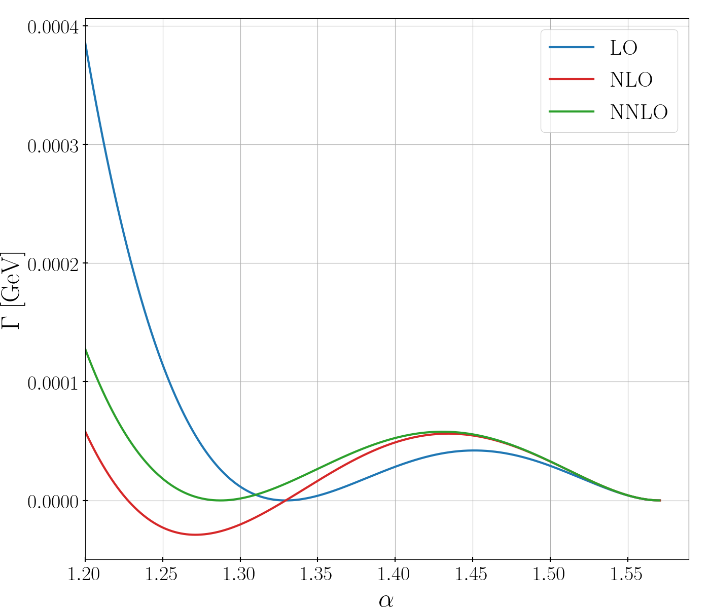
Figure 2: Partial decay width $\Gamma(h_{2}\to h_{1}h_{1})$ for the benchmark point BPapprox as a function of the mixing angle $\alpha$, at LO (blue), NLO (orange), and approximate NNLO (green).

4 Implementation in sHDECAY: EWsHDECAY

We implemented the EW one-loop corrections to the Higgs decays derived in this work in the singlet extension sHDECAY of the code HDECAY [6, 7] where we updated the underlying HDECAY version to version 6.61. The resulting code is called EWsHDECAY. Note, that we impose an extra $\mathbb{Z}_{2}$ symmetry on $S$ in contrast to the CxSM version implemented in sHDECAY [8]. In order to use our version of the CxSM therefore the input parameter $a_{1}$ has to be set to zero in the input file, cf. also footnote 5. The Fortran code HDECAY and thereby its extension sHDECAY include the state-of-the-art QCD corrections to the partial decay widths. For the consistent combination of our EW corrections with HDECAY which uses the Fermi constant $G_{F}$ as input parameter, we use the $G_{\mu}$, respectively the $G_{F}$ scheme, in the definition of our counterterm for the electric charge, cf. Subsection 3.1.2.

Note, that sHDECAY also calculates the off-shell decays into final states with an off-shell top-quark $t^{*}$, $\phi\to t^{*}\bar{t}$ ($\phi=h_{1},h_{2}$) and into final states with off-shell gauge bosons $V^{*}$ ($V=W,Z$), $\phi\to V^{*}V^{*}$. The EW corrections are only computed for on-shell decays, however. This means that if only off-shell decays are kinematically allowed for the mentioned final states, then the EW corrections are not included and only the LO decay width is calculated. Be reminded also, that we did not include EW corrections to the loop-induced decays into photonic and gluonic final states. We furthermore assume that the QCD and EW corrections factorize. The relative QCD corrections $\delta^{\text{QCD}}$ are defined relative to the LO width $\Gamma^{\text{CxSM,LO}}$ calculated by sHDECAY, which contains (where applicable) running quark masses in order to improve the perturbative behavior. The relative EW corrections $\delta^{\text{EW}}$ on the other hand, are obtained by normalizing to the LO width with OS particle masses. The QCD and EW corrected decay width into a specific OS and non-loop-induced final state, $\Gamma^{\text{QCD\&EW}}$ is hence obtained as

$$\Gamma^{\text{QCD\&EW}}=\Gamma^{\text{CxSM,LO}}[1+\delta^{\text{QCD}}][1+\delta^{\text{EW}}]=\Gamma^{\text{CxSM,QCD}}[1+\delta^{\text{EW}}]\;.$$ (30)

And the branching ratio of the higher-order (HO) corrected decay width $h_{i}$ ($i=1,2$) into a specific final state is calculated by

$$\mbox{BR}(h_{i}\to XX)=\frac{\Gamma^{\text{HO}}(h_{i}\to XX)}{\Gamma_{\text{tot}}^{\text{QCD\&EW}}}\;,$$ (31)

with the total width given by,

$$\Gamma_{\text{tot}}^{\text{QCD\&EW}}(h_{i}) = \Gamma^{\text{QCD}}(h_{i}\to gg)+\Gamma(h_{i}\to\gamma\gamma)$$

$$+\sum_{f=s,c,b,t}\Gamma^{\text{QCD\&EW}}(h_{i}\to ff)+\Gamma^{\text{EW}}(h_{i}\to\tau\tau)$$

$$+\sum_{V=Z,W}\Gamma^{\text{EW}}(h_{i}\to VV)+\delta_{i2}\Gamma^{\text{EW}}(h_{2}\to h_{1}h_{1})+\Gamma^{\text{EW}}(h_{i}\to AA)\;.$$

As mentioned above, the QCD corrections to the decays into colored final states are those as implemented in the original HDECAY version, for details see [7]. As mentioned above, the EW corrections are only included for non-loop-induced final states and for on-shell decays. Otherwise the off-shell tree-level decays are used if implemented in sHDECAY, as is the case for the $tt$, $ZZ$ and $WW$ final states, hence

$$\Gamma^{\text{EW}}(h_{i}\to XX)=\left\{\begin{array}[]{lcl}\Gamma^{\text{EW}}(h_{i}\to XX)&\mbox{for}&m_{h_{i}}\geq 2m_{X}\\ \Gamma^{\text{LO}}(h_{i}\to X^{*}X^{*})&\mbox{for}&m_{h_{i}}<2m_{X}\end{array}\right.\;,\quad\mbox{with }X=t,Z,W\;,$$ (35)

and

$$\Gamma^{\text{EW}}(h_{i}\to XX)=\left\{\begin{array}[]{lcl}\Gamma^{\text{EW}}(h_{i}\to XX)&\mbox{for}&m_{h_{i}}\geq 2m_{X}\\ 0&\mbox{for}&m_{h_{i}}<2m_{X}\end{array}\right.\;,\quad\mbox{with }X=b,\tau,h_{1},A\;.$$ (38)

Note, that for the fermionic final states we included the EW corrections only of the third generation. As the decay widths in fermion pairs of the first two generations are much smaller, the effect of not including the EW corrections here is negligible. The partial widths $\Gamma^{\text{HO}}(h_{i}\to XX)$ in Eq. (31) are given as defined in Eqs. (30) to (38).

The parameters of the model are set in the corresponding block of the input file hdecay.in as in the original input file for sHDECAY.

********************** real or complex singlet Model *********************
Singlet Extension: 1 - yes, 0 - no (based on SM w/o EW corrections)
Model: 1 - real broken phase, 2 - real dark matter phase
       3 - complex broken phase, 4 - complex dark matter phase
isinglet = 1
icxSM    = 4
...
*** complex singlet dark matter phase ***
alph1    = -0.14331719167196D0
m1       = 125.09D0
m2       = 345.0021536863908D0
m3       = 61.02910887468706D0
vs       = 467.196443135993D0
a1       = 0.D0

The model for which we compute the EW corrections is the CxSM in the DM phase, so that the user has to choose ’icxSM=4’ after setting ’isinglet=1’. The input values are then given in the block named ’complex singlet dark matter phase’. We consider a specific version of the model where the parameter $a_{1}$ does not appear in the model, so that it has to be set to 0 for the computation of the EW corrections. Therefore, if the parameter is chosen to be non-zero, no EW corrections will be calculated. Note, that $m_{1,2}$ denote the lighter and heavier of the two visible Higgs boson masses, and $m_{3}$ is the mass value of the DM particle. For the inclusion of the EW corrections the input file hdecay.in of sHDECAY has been extended by the following lines:

******************** EW Corrections ********************
** Attention: This can only be used for the complex dark matter phase
(icxSM=4) of the CxSM with a1 = 0 **
**** ielwcxsm = 0 LO, = 1 include NLO corrections
ielwcxsm = 1
**** ren. scheme: vsscheme = 1 pd, = 2 ZEM, pdprocess = 1 h1->AA, =2
h2->AA, alpha_mix =1 OS, =2 pstar
vsscheme = 2
pdprocess= 2
ralph_mix= 1
**** IR parameter - DeltaE is the detector resolution (in GeV)
DeltaE   = 10.0D0
**** NNLO approx: NNLOapprox=1, add NLO^2 term to h2h1h1 decay width
if |tan(alpha)*(v/vs)-1|<deltaNNLO
NNLOapp  = 1
deltaNNLO= 0.05D0
**** Parameter conversion, change input parameters vS and alpha
accordingly, if given scheme above is not the specified input scheme
**** Paramcon = 0 no parameter conversion, =1 do parameter conversion
**** Standard scheme: stdvs = 1 pd, = 2 ZEM, stdproc = 1 h1->AA,
=2 h2->AA, stdalpha =1 OS, =2 pstar
Paramcon = 0
stdvs    = 1
stdproc  = 2
stdalpha = 1

The warning reminds the user that our computation of the EW corrections only applies to the CxSM in the DM phase with the $a_{1}=0$ in the potential. By setting the input parameter ’ielwcxsm’ equal to 1 (0), the EW corrections will be computed (omitted). The next three parameters choose the applied renormalization scheme. Setting ’vsscheme’ to 1, the singlet VEV counterterm will be computed in the process-dependent scheme using the on-shell decay $h_{1}\to AA$ ($h_{2}\to AA$) by choosing ’pdprocess =1 (2)’ (called ’OSproc1’ and ’OSproc2’, respectively, in Tab. 1). When ’vsscheme’ is set to 2, then the process-dependent renormalization scheme for $v_{s}$ is evaluated at zero external momenta for the chosen decay process (called ’ZEMproc1’ and ’ZEMproc2’, respectively in Tab. 1). With ’ralph_mix=1 (2)’ the OS-pinched ($p_{*}$-pinched) scheme is chosen for the renormalization of the mixing angle $\alpha$.

The next parameter setting chooses with ’DeltaE’ the detector resolution needed in the computation of the IR corrections, which we set by default equal to 10 GeV, cf. [9]. The following two parameters concern the computation of the NNLO corrections to the decay width $h_{2}\to h_{1}h_{1}$. If ’NNLOapp’ is set equal to 1 then the NNLO width is computed for parameter configurations with $\tan\alpha$ values in the vicinity of $v_{S}/v$, namely $\tan\alpha\in\{v_{s}/v-\mbox{deltaNNLO},v_{s}/v+\mbox{deltaNNLO}\}$. Be aware, however, that for $\tan\alpha\neq v_{s}/v$, the NNLO computation is incomplete, as discussed above.

The last four parameters refer to the conversion of the input parameters. The change of the renormalization scheme allows for an estimate of the uncertainty in the NLO EW corrections due to the missing higher-order corrections. For such an estimate to be meaningful also the input parameters have to be changed consistently. For the conversion of the input parameters, when going from one to the other renormalization scheme, our code uses an approximate formula based on the bare parameter $p_{0}$ which is independent of the scheme so that,

$$p_{\text{spec}}=p_{\text{std}}+\delta p_{\text{std}}-\delta p_{\text{spec}}\;,$$ (39)

where $p_{x}$ and $\delta p_{x}$ denote the renormalized parameter $p$ and its counterterm $\delta p$ in the standard scheme and in the user specified scheme, respectively. Setting the flag ’ Paramcon = 1’, the parameter conversion is applied. In this case, the user can then also choose which renormalization scheme is the ’standard’ scheme, by setting the three parameters ’(stdvs,stdproc,stdalpha)’. If the user specified renormalization scheme ’(vsscheme,pdprocess,ralph)’ and the standard scheme ’(stdvs,stdproc,stdalpha)’ are identical, the input parameters $v_{S}$ and $\alpha$ remain unchanged. Otherwise they are converted from their values understood to be given in the standard scheme ’(stdvs,stdproc,stdalpha)’ to the values they take in the user specified scheme ’(vsscheme,pdprocess,ralph)’. The converted parameter values are given out in the file ’Paramconversion.txt’. If, however, the user chooses ’Paramcon = 0’ the parameters are not converted when the specified renormalization scheme differs from the standard scheme. In this case a comparison of the results for different renormalization schemes to estimate the theoretical uncertainty would not, however, be meaningful.

Note that we do not give out the NLO value of a specific decay width if it becomes negative. In this case, and also if a chosen renormalization scheme cannot be applied because it is kinematically not allowed, the decay width is computed and given out at LO in the EW corrections together with a warning. Remark, finally, that when we take the SM limit of our model and compare the results for the EW corrections to those obtained from HDECAY for the SM, we differ in the decay into gauge boson final states as HDECAY includes the EW corrections also to the off-shell SM Higgs decays into $WW/ZZ$ and to the loop-induced decays into gluon and photon pairs.

The code can be downloaded at the url:

https://github.com/fegle/ewshdecay

Apart from short explanations and user instructions, we also provide sample input and output files on this webpage.

5 Parameter Scan

In order to obtain viable parameter points for our numerical analysis we performed a scan in the parameter space of the model and kept only those points which fulfill the relevant theoretical and experimental constraints described below. They are checked for by ScannerS [42, 43] which we used for the parameter scan, with the scan ranges summarized in Tab. 2.

Parameter	Range
	Lower	Upper
$m_{s}$	30 GeV	1000 GeV
$m_{A}$	10 GeV	1000 GeV
$v_{S}$	1 GeV	1000 GeV
$\alpha$	$-$1.57	1.57

Table 2: The scan ranges used for the generation of parameter points with ScannerS. The mass $m_{s}$ denotes the scalar mass of the non-125 GeV Higgs boson.

The values of the SM input parameters needed for our calculation are given in Tab. 3. These are the values suggested by the LHC Higgs Working Group [44].

SM parameter	Value
$m_{Z}$	91.15348 GeV
$m_{W}$	80.3579 GeV
$m_{h_{125}}$	125.09 GeV
$m_{\tau}$	1.77682 GeV
$\overline{m}_{b}(m_{b})$	4.18 GeV
$m_{t}$	172.5 GeV

Table 3: The SM parameter values used in the numerical evaluation taken from [45] and following the recommendations of [44]. Here, $\overline{m}_{b}$ denotes the $\overline{\mbox{MS}}$ bottom quark mass which is taken at the scale of the bottom quark mass, $m_{b}$, and $h_{125}$ denotes the SM-like Higgs boson with a mass of 125.09 GeV.

The theoretical constraints that are taken into account are boundedness from below, perturbative unitarity and stability of the vacuum. For detailed information, we refer to [3].

As for the experimental constraints, we first note that in our model the $\rho$ parameter is equal to 1 at tree level and there are no tree-level flavour-changing neutral currents, as the gauge singlet does not couple to fermions and gauge bosons in the gauge basis. We check for compatibility with EW precision data by requiring the $S,T,U$ parameters [47] to be consistent with the measured quantities at 95% confidence level. Compatibility with the LHC Higgs data and exclusion bounds is checked through the ScannerS link with HiggsSignals [48, 49] and HiggsBounds [50, 51]. We require the signal rates of our SM-like Higgs boson to be in agreement with the experimental data at the $2\sigma$ level. Through the link with MicrOmegas [52] we ensure that the DM relic density of our model does not exceed the measured value. Concerning DM direct detection, the tree-level cross section is negligible in this model [53, 54], but the loop-corrected DM-nucleon spin-independent cross section [55, 56] has to be checked to be below the experimental bounds [57, 58, 59] with the most stringent bounds given by the LUX-ZEPLIN experiment [59]. Further detailed information on the experimental constraints that we applied is given in [3].

In our sample we take off parameter scenarios where the deviation of any other neutral scalar mass from the $h_{125}$ mass is below 2.5 GeV. This suppresses interfering di-Higgs signals which would require a further special treatment to correctly consider theory and experiment beyond the scope and focus of the present work.

We also used the program BSMPT [60, 61] to check if the thus obtained parameter sample leads to vacuum states compatible with an EW VEV $v=246$ GeV also at NLO, i.e. after including higher-order corrections to the effective potential. Provided this to be the case, we checked if we have points providing a strong first-order EW phase transition (SFOEWPT), one of the Sakharov conditions [62] to be fulfilled for EW baryogenesis. We found that none of the parameter points with a viable NLO EW vacuum provides an SFOEWPT.

Finally, we applied constraints from the resonant di-Higgs searches performed by the LHC experiments. We proceed here as described in [63] to which we also refer for a detailed description, giving here only the most important points. In order to apply the constraints, we calculated for parameter points of scenario I, where $m_{h_{2}}>2m_{h_{1}}\equiv 2m_{h_{125}}$ the production cross section $\sigma(h_{2})$ at next-to-next-to-leading-order QCD using the code SusHi v1.6.1 [64, 65, 66] and multiplied it with the branching ration $\mbox{BR}(h_{2}\to h_{1}h_{1})$. We then checked if the thus obtained rate is below the experimental values given in Refs. [67, 68, 69] for the $4b$, [70, 71, 72] for the $(2b)(2\tau)$, [73, 74] for the $(2b)(2\gamma)$, [75] for the $(2b)(2W)$, [76] for the $(2b)(ZZ)$, [77] for the $(2W)(2\gamma)$ and [78] for the $4W$ final states. There are also experimental limits from non-resonant searches. They do not constrain our model so far, however, as will be discussed below.

The parameter points which are found to be compatible with all applied constraints can be divided up into two samples, depending on which of the visible Higgs particles is the SM-like one, called $h_{125}$ in the following. For the two samples, we will adopt the following notation,

$$\begin{array}[]{ll}m_{h_{1}}=m_{h_{125}}:&\mbox{ scenario I}\\ m_{h_{2}}=m_{h_{125}}:&\mbox{ scenario II}\;.\end{array}$$ (42)

6 Numerical Analysis

We start our numerical analysis by investigating what is the impact of our extended scan compared to [3] on the allowed parameter regions of the model. We move on to the discussion of the overall size of the computed EW corrections before investigating the remaining theoretical uncertainty due to missing higher-order corrections. We then discuss the phenomenological impact of these corrections w.r.t the Higgs decays into DM particles and the impact on the allowed parameter regions. Finally, we investigate Higgs pair production in the context of our model and how it is affected by our corrections.

6.1 Allowed Parameter Regions and DM Observables

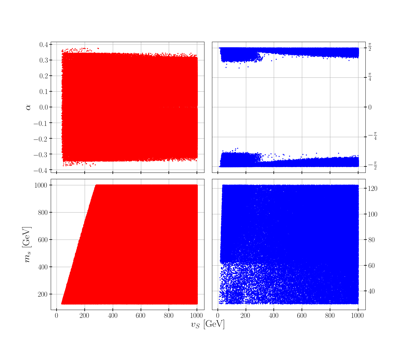
Figure 3: Allowed input parameters $\alpha$ vs. $v_{S}$ (upper row) and $m_{S}$ vs. $v_{S}$ (lower row). Left: for scenario I ($h_{1}=h_{125}$, red points); right: for scenario II ($h_{2}=h_{125}$, blue points).

In our new scan we go up to $m_{A}$ values of 1 TeV, as compared to [3], we now also allow for scenarios where the decay of the SM-like Higgs boson into DM particles is kinematically closed. This leads to an enlarged parameter space, a larger variation in the particle couplings and masses and hence effects in the NLO EW corrections that would not appear in the more restricted sample. We therefore show the corresponding plot to Fig. 1 in [3]. Figure 3 (upper) displays the allowed combinations of $\alpha$ and $v_{S}$ for scenario I, i.e. $h_{1}=h_{125}$, (left) and for scenario II, i.e. $h_{2}=h_{125}$, (right). The lower plot shows the corresponding values of non-125-GeV Higgs boson mass $m_{S}$ vs. $v_{S}$. Compared to [3], we see that $\alpha$ and $v_{S}$ are not linked any more as for the large DM matter masses, that are now included in our scan, the kinematic constraints inducing this relation are not applicable any more. This leads also to a larger allowed maximum range for $|\alpha|$ which has increased in scenario I from about 0.27 to about 0.34 for almost all parameter points of scenario I. This is the maximal allowed value compatible with the Higgs data except for parameter points where the visible Higgs bosons are close in mass and the Higgs signal is built up by the two Higgs bosons. These are the outliers with larger mixing angles up to about 0.37. If we dropped the exclusion of parameter points with non-SM-Higgs masses closer than 2.5 GeV to the SM-like Higgs mass then the mixing could be even larger. Also in scenario II larger deviations from $\alpha=\pm\pi/2$ are possible for the increased parameter scan. The lower plots, apart from becoming more dense, did not change the shape. The perturbative unitarity constraints are reflected in the linear relation between $m_{S}$ and $v_{S}$, cf. the discussion in [3].

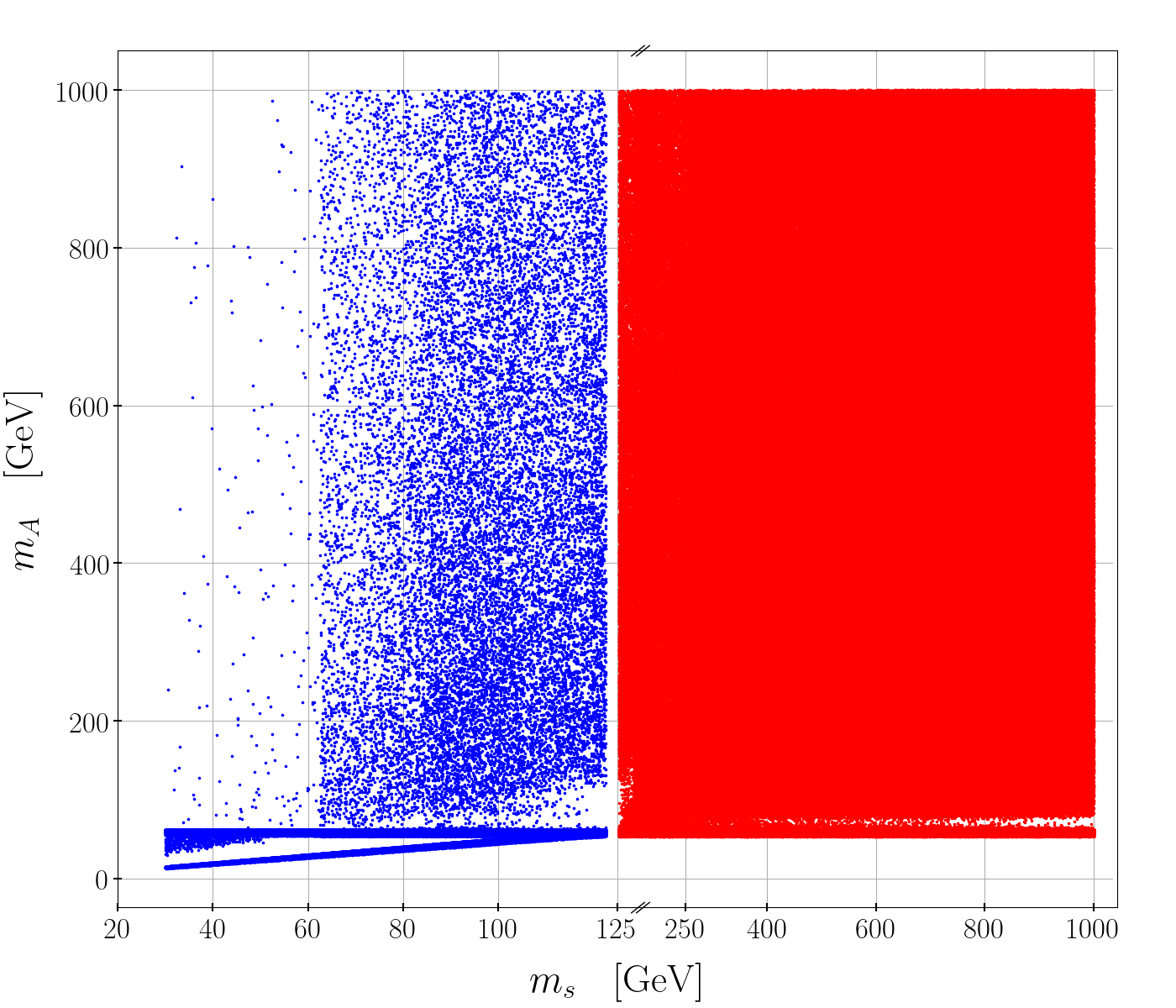
Figure 4: Allowed DM mass values $m_{A}$ versus non-SM-like Higgs mass values $m_{S}$ in GeV for scenario II ($h_{2}=h_{125}$, blue points) and scenario I ($h_{1}=h_{125}$, red points).

Figure 4 displays the allowed values of the DM mass $m_{A}$ versus the non-SM-like Higgs mass mass $m_{S}$ for scenario I (red points) and scenario II (blue points). For $m_{A}$ values below 62.5 GeV, only mass values in the vicinity of $m_{h_{125}}/2$ or $m_{S}/2$ are allowed, as then efficient DM annihilation via $h_{125}$ or the non-SM-like Higgs particle can take place such that the DM relic density constraints can be met (cf. our discussion in [3]). For large $m_{A}$ values where annihilation via other SM particles can take place all mass values up to the upper limit of our scan are allowed.

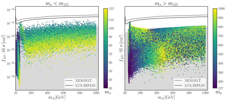
Figure 5: Effective spin-independent nucleon DM cross section as a function of the DM mass for scenario II (left) and scenario I (right). The limits from XENON1T [57] and LUX-ZEPLIN [59] are given by the dashed and full line, respectively. The grey shaded region corresponds to the neutrino floor. The color code represents the non-SM-like Higgs mass value in GeV.

In Fig. 5 we show the effective spin-independent nucleon DM detection cross section as a function of the DM mass $m_{A}$ for scenario II (left) and scenario I (right). The multiplication of the spin-independent cross section SI $\sigma$ with the factor

$$f_{AA}=\frac{(\Omega h^{2})_{A}}{(\Omega h^{2})^{\text{obs}}_{\text{DM}}}$$ (43)

accounts for the fact that the relic density $(\Omega h^{2})_{A}$ of our DM candidate $A$ might not account for the entire observed DM relic density $(\Omega h^{2})^{\text{obs}}_{\text{DM}}=0.120\pm 0.001$ [79]. In our model the direct detection cross section at LO is negligible due to a cancellation [53, 54] so that we present the one-loop result calculated in [55, 56]. In [3], we made a mistake that we correct here so that now both the exclusion limits from Xenon1T [57] (dashed) and LUX-ZEPLIN [59] (full) as well as the neutrino floor (grey region) move down by one order of magnitude. The effect is that for both scenarios I and II we have now parameter points above the neutrino floor that can hence be tested by direct detection experiments. Moreover, we find that in the parameter region $m_{A}\geq m_{h_{125}}/2$, where we cannot probe DM at the LHC, the LUX-ZEPLIN experiment [59] is sensitive to the model in the region $66\mbox{ GeV }\mathrel{\hbox to0.0pt{\lower 4.0pt\hbox{\hskip 1.0pt$\sim$}\hss}\raise 1.0pt\hbox{$<$}}m_{A}\mathrel{\hbox to0.0pt{\lower 4.0pt\hbox{\hskip 1.0pt$\sim$}\hss}\raise 1.0pt\hbox{$<$}}78$ GeV. Future increased precision in the direct detection experiments will allow to test the model in (large) parts of the still allowed $m_{A}$ range in scenario I (scenario II).

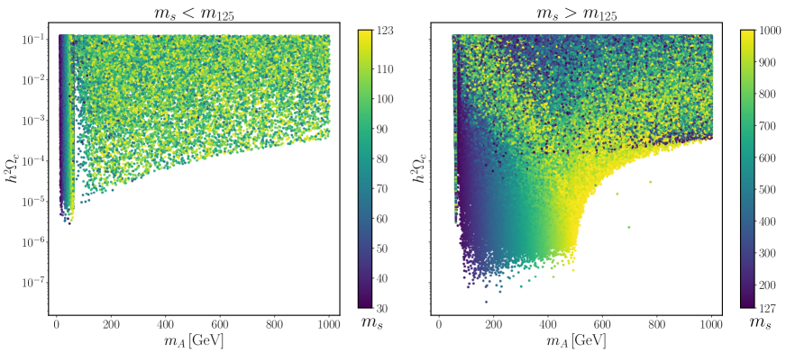
Figure 6: Relic density as a function of the DM mass $m_{A}$ for both II (left) and scenario I (right). The color code represents the non-SM-like Higgs mass value in GeV.

Figure 6 displays the relic density for all points passing our constraints for scenario II (left) and scenario I (right). As can be inferred from the plot for the whole allowed region up to $m_{A}=1$ TeV, where our scan ends, there are parameter scenarios that saturate the relic density.

6.2 Size of NLO EW Corrections

	OSproc1-OS		OSproc1-$p_{*}$		OSproc2-OS		OSproc2-$p_{*}$
	Min	Max	Min	Max	Min	Max	Min	Max
$h_{1}\to bb$	$-1.45\text{\,}\mathrm{\char 37\relax}$	$0.0\text{\,}\mathrm{\char 37\relax}$	$-1.41\text{\,}\mathrm{\char 37\relax}$	$0.0\text{\,}\mathrm{\char 37\relax}$	$-4.66\text{\,}\mathrm{\char 37\relax}$	$0.0\text{\,}\mathrm{\char 37\relax}$	$-4.79\text{\,}\mathrm{\char 37\relax}$	$0.0\text{\,}\mathrm{\char 37\relax}$
$h_{1}\to\tau\tau$	$-4.65\text{\,}\mathrm{\char 37\relax}$	$0.0\text{\,}\mathrm{\char 37\relax}$	$-4.61\text{\,}\mathrm{\char 37\relax}$	$0.0\text{\,}\mathrm{\char 37\relax}$	$-7.85\text{\,}\mathrm{\char 37\relax}$	$0.0\text{\,}\mathrm{\char 37\relax}$	$-7.99\text{\,}\mathrm{\char 37\relax}$	$0.0\text{\,}\mathrm{\char 37\relax}$
$h_{1}\to AA$	$0\text{\,}\mathrm{\char 37\relax}$	$0\text{\,}\mathrm{\char 37\relax}$	$0\text{\,}\mathrm{\char 37\relax}$	$0\text{\,}\mathrm{\char 37\relax}$	$-2.12\text{\,}\mathrm{\char 37\relax}$	$6.78\text{\,}\mathrm{\char 37\relax}$	$-2.24\text{\,}\mathrm{\char 37\relax}$	$7.18\text{\,}\mathrm{\char 37\relax}$
$h_{2}\to bb$	$-9.19\text{\,}\mathrm{\char 37\relax}$	$4.85\text{\,}\mathrm{\char 37\relax}$	$-9.57\text{\,}\mathrm{\char 37\relax}$	$5.26\text{\,}\mathrm{\char 37\relax}$	$-10.18\text{\,}\mathrm{\char 37\relax}$	$19.72\text{\,}\mathrm{\char 37\relax}$	$-10.52\text{\,}\mathrm{\char 37\relax}$	$25.06\text{\,}\mathrm{\char 37\relax}$
$h_{2}\to\tau\tau$	$-16.3\text{\,}\mathrm{\char 37\relax}$	$0.0\text{\,}\mathrm{\char 37\relax}$	$-16.79\text{\,}\mathrm{\char 37\relax}$	$0.0\text{\,}\mathrm{\char 37\relax}$	$-19.03\text{\,}\mathrm{\char 37\relax}$	$16.39\text{\,}\mathrm{\char 37\relax}$	$-19.5\text{\,}\mathrm{\char 37\relax}$	$21.74\text{\,}\mathrm{\char 37\relax}$
$h_{2}\to tt$	$-6.17\text{\,}\mathrm{\char 37\relax}$	$5.47\text{\,}\mathrm{\char 37\relax}$	$-6.17\text{\,}\mathrm{\char 37\relax}$	$6.13\text{\,}\mathrm{\char 37\relax}$	$-6.16\text{\,}\mathrm{\char 37\relax}$	$11.05\text{\,}\mathrm{\char 37\relax}$	$-6.16\text{\,}\mathrm{\char 37\relax}$	$10.93\text{\,}\mathrm{\char 37\relax}$
$h_{2}\to WW$	$-9.82\text{\,}\mathrm{\char 37\relax}$	$9.31\text{\,}\mathrm{\char 37\relax}$	$-9.85\text{\,}\mathrm{\char 37\relax}$	$9.5\text{\,}\mathrm{\char 37\relax}$	$-9.8\text{\,}\mathrm{\char 37\relax}$	$19.49\text{\,}\mathrm{\char 37\relax}$	$-9.89\text{\,}\mathrm{\char 37\relax}$	$21.53\text{\,}\mathrm{\char 37\relax}$
$h_{2}\to ZZ$	$-3.53\text{\,}\mathrm{\char 37\relax}$	$4.44\text{\,}\mathrm{\char 37\relax}$	$-3.51\text{\,}\mathrm{\char 37\relax}$	$5.27\text{\,}\mathrm{\char 37\relax}$	$-3.54\text{\,}\mathrm{\char 37\relax}$	$12.1\text{\,}\mathrm{\char 37\relax}$	$-3.59\text{\,}\mathrm{\char 37\relax}$	$13.33\text{\,}\mathrm{\char 37\relax}$
$h_{2}\to h_{1}h_{1}$	$-14.14\text{\,}\mathrm{\char 37\relax}$	$10.64\text{\,}\mathrm{\char 37\relax}$	$-14.04\text{\,}\mathrm{\char 37\relax}$	$10.54\text{\,}\mathrm{\char 37\relax}$	$-99.4\text{\,}\mathrm{\char 37\relax}$	$>$$100\text{\,}\mathrm{\char 37\relax}$	$-98.24\text{\,}\mathrm{\char 37\relax}$	$>$$100\text{\,}\mathrm{\char 37\relax}$
$h_{2}\to AA$	$-6.75\text{\,}\mathrm{\char 37\relax}$	$2.14\text{\,}\mathrm{\char 37\relax}$	$-7.2\text{\,}\mathrm{\char 37\relax}$	$2.25\text{\,}\mathrm{\char 37\relax}$	$0\text{\,}\mathrm{\char 37\relax}$	$0\text{\,}\mathrm{\char 37\relax}$	$0\text{\,}\mathrm{\char 37\relax}$	$0\text{\,}\mathrm{\char 37\relax}$
	ZEMproc1-OS		ZEMproc1-$p_{*}$		ZEMproc2-OS		ZEMproc2-$p_{*}$
	Min	Max	Min	Max	Min	Max	Min	Max
$h_{1}\to bb$	$-4.66\text{\,}\mathrm{\char 37\relax}$	$-0.88\text{\,}\mathrm{\char 37\relax}$	$-4.79\text{\,}\mathrm{\char 37\relax}$	$-0.62\text{\,}\mathrm{\char 37\relax}$	$-4.66\text{\,}\mathrm{\char 37\relax}$	$-0.88\text{\,}\mathrm{\char 37\relax}$	$-4.79\text{\,}\mathrm{\char 37\relax}$	$-0.62\text{\,}\mathrm{\char 37\relax}$
$h_{1}\to\tau\tau$	$-7.85\text{\,}\mathrm{\char 37\relax}$	$-4.08\text{\,}\mathrm{\char 37\relax}$	$-7.99\text{\,}\mathrm{\char 37\relax}$	$-3.8\text{\,}\mathrm{\char 37\relax}$	$-7.85\text{\,}\mathrm{\char 37\relax}$	$-4.08\text{\,}\mathrm{\char 37\relax}$	$-7.99\text{\,}\mathrm{\char 37\relax}$	$-3.8\text{\,}\mathrm{\char 37\relax}$
$h_{1}\to AA$	$-3.5\text{\,}\mathrm{\char 37\relax}$	$5.76\text{\,}\mathrm{\char 37\relax}$	$-3.5\text{\,}\mathrm{\char 37\relax}$	$5.76\text{\,}\mathrm{\char 37\relax}$	$-4.63\text{\,}\mathrm{\char 37\relax}$	$9.51\text{\,}\mathrm{\char 37\relax}$	$-5.0\text{\,}\mathrm{\char 37\relax}$	$9.93\text{\,}\mathrm{\char 37\relax}$
$h_{2}\to bb$	$-99.94\text{\,}\mathrm{\char 37\relax}$	$19.77\text{\,}\mathrm{\char 37\relax}$	$-99.57\text{\,}\mathrm{\char 37\relax}$	$25.04\text{\,}\mathrm{\char 37\relax}$	$-99.94\text{\,}\mathrm{\char 37\relax}$	$19.71\text{\,}\mathrm{\char 37\relax}$	$-99.57\text{\,}\mathrm{\char 37\relax}$	$25.06\text{\,}\mathrm{\char 37\relax}$
$h_{2}\to\tau\tau$	$-99.32\text{\,}\mathrm{\char 37\relax}$	$16.37\text{\,}\mathrm{\char 37\relax}$	$-98.96\text{\,}\mathrm{\char 37\relax}$	$21.7\text{\,}\mathrm{\char 37\relax}$	$-99.32\text{\,}\mathrm{\char 37\relax}$	$16.38\text{\,}\mathrm{\char 37\relax}$	$-98.96\text{\,}\mathrm{\char 37\relax}$	$21.73\text{\,}\mathrm{\char 37\relax}$
$h_{2}\to tt$	$-99.28\text{\,}\mathrm{\char 37\relax}$	$11.06\text{\,}\mathrm{\char 37\relax}$	$-99.11\text{\,}\mathrm{\char 37\relax}$	$10.93\text{\,}\mathrm{\char 37\relax}$	$-99.28\text{\,}\mathrm{\char 37\relax}$	$11.02\text{\,}\mathrm{\char 37\relax}$	$-99.11\text{\,}\mathrm{\char 37\relax}$	$10.91\text{\,}\mathrm{\char 37\relax}$
$h_{2}\to WW$	$-98.69\text{\,}\mathrm{\char 37\relax}$	$19.46\text{\,}\mathrm{\char 37\relax}$	$-98.81\text{\,}\mathrm{\char 37\relax}$	$21.55\text{\,}\mathrm{\char 37\relax}$	$-98.69\text{\,}\mathrm{\char 37\relax}$	$19.45\text{\,}\mathrm{\char 37\relax}$	$-98.81\text{\,}\mathrm{\char 37\relax}$	$21.52\text{\,}\mathrm{\char 37\relax}$
$h_{2}\to ZZ$	$-98.18\text{\,}\mathrm{\char 37\relax}$	$12.08\text{\,}\mathrm{\char 37\relax}$	$-97.8\text{\,}\mathrm{\char 37\relax}$	$13.29\text{\,}\mathrm{\char 37\relax}$	$-98.18\text{\,}\mathrm{\char 37\relax}$	$12.06\text{\,}\mathrm{\char 37\relax}$	$-97.8\text{\,}\mathrm{\char 37\relax}$	$13.32\text{\,}\mathrm{\char 37\relax}$
$h_{2}\to h_{1}h_{1}$	$-99.95\text{\,}\mathrm{\char 37\relax}$	$>$$100\text{\,}\mathrm{\char 37\relax}$	$-99.96\text{\,}\mathrm{\char 37\relax}$	$>$$100\text{\,}\mathrm{\char 37\relax}$	$-99.92\text{\,}\mathrm{\char 37\relax}$	$>$$100\text{\,}\mathrm{\char 37\relax}$	$-99.88\text{\,}\mathrm{\char 37\relax}$	$>$$100\text{\,}\mathrm{\char 37\relax}$
$h_{2}\to AA$	$-100.0\text{\,}\mathrm{\char 37\relax}$	$5.65\text{\,}\mathrm{\char 37\relax}$	$-100.0\text{\,}\mathrm{\char 37\relax}$	$5.82\text{\,}\mathrm{\char 37\relax}$	$-15.22\text{\,}\mathrm{\char 37\relax}$	$9.03\text{\,}\mathrm{\char 37\relax}$	$-15.23\text{\,}\mathrm{\char 37\relax}$	$9.09\text{\,}\mathrm{\char 37\relax}$

Table 4: Scenario I: Relative NLO corrections $\delta_{\text{EW}}(h_{i}\to XX)$ for all possible decay processes in scenario I, i.e. $m_{h_{1}}=125.09$ GeV, and different renormalization schemes $\mbox{ren}_{v_{S}}$-$\mbox{ren}_{\alpha}$. For $\delta v_{S}$ we have OS renormalization and ZEM renormalization in the two possible processes, $\mbox{ren}_{v_{S}}=$ OSproc1, OSproc2, ZEMproc1, ZEMproc2. For $\delta\alpha$ we have the two possible schemes $\mbox{ren}_{\alpha}=$ OS, $p_{*}$. The renormalization schemes and their notation are summarized in Tab. 1.

In Tab. 4 we show the relative NLO corrections to the partial widths $\Gamma$ of the decay of $h_{i}$ ($i=1,2$) into the various possible final states $XX$ ($X=\tau,b,t,W,Z,A,h_{1}$), defined as

$$\delta_{\text{EW}}(h_{i}\to XX)=\frac{\Gamma^{\text{NLO}}_{h_{i}\to XX}-\Gamma^{\text{LO}}_{h_{i}\to XX}}{\Gamma^{\text{LO}}_{h_{i}\to XX}}\,,$$ (44)

for scenario I (Tab. 4) and scenario II (Tab. 5) and different renormalization schemes. These are for the renormalization of the singlet VEV $v_{S}$ the process-dependent and the ZEM scheme, using either the $h_{1}\to AA$ or $h_{2}\to AA$ decay and for the renormalization of $\alpha$ the OS- or the $p_{\star}$-pinched scheme. The notation for the schemes is summarized in Tab. 1. We also note that we discard all parameter points where the large relative corrections are beyond -100%, in order to not encounter unphysical results with negative decay widths at NLO. We furthermore emphasize that the results given in a specific renormalization scheme assume the input parameters to be given in this specific renormalization scheme. We hence do not start from a certain scheme $a$ and then move on to a different scheme $b$ by consistently converting the input parameters of scheme $a$ to scheme $b$. The results given in the various schemes hence have to be looked at and discussed each one by one. They are meant to give an overview of what sizes of corrections can be expected in the various schemes.

	OSproc1-OS		OSproc1-$p_{*}$		OSproc2-OS		OSproc2-$p_{*}$
	Min	Max	Min	Max	Min	Max	Min	Max
$h_{1}\to bb$	$-1.37\text{\,}\mathrm{\char 37\relax}$	$6.02\text{\,}\mathrm{\char 37\relax}$	$-1.68\text{\,}\mathrm{\char 37\relax}$	$0.81\text{\,}\mathrm{\char 37\relax}$	$-49.18\text{\,}\mathrm{\char 37\relax}$	$27.16\text{\,}\mathrm{\char 37\relax}$	$-48.31\text{\,}\mathrm{\char 37\relax}$	$37.35\text{\,}\mathrm{\char 37\relax}$
$h_{1}\to\tau\tau$	$-4.47\text{\,}\mathrm{\char 37\relax}$	$5.32\text{\,}\mathrm{\char 37\relax}$	$-4.48\text{\,}\mathrm{\char 37\relax}$	$1.68\text{\,}\mathrm{\char 37\relax}$	$-52.03\text{\,}\mathrm{\char 37\relax}$	$26.52\text{\,}\mathrm{\char 37\relax}$	$-51.16\text{\,}\mathrm{\char 37\relax}$	$37.53\text{\,}\mathrm{\char 37\relax}$
$h_{1}\to AA$	$0\text{\,}\mathrm{\char 37\relax}$	$0\text{\,}\mathrm{\char 37\relax}$	$0\text{\,}\mathrm{\char 37\relax}$	$0\text{\,}\mathrm{\char 37\relax}$	$-5.57\text{\,}\mathrm{\char 37\relax}$	$3.63\text{\,}\mathrm{\char 37\relax}$	$-1.24\text{\,}\mathrm{\char 37\relax}$	$5.16\text{\,}\mathrm{\char 37\relax}$
$h_{2}\to bb$	$-1.39\text{\,}\mathrm{\char 37\relax}$	$0.0\text{\,}\mathrm{\char 37\relax}$	$-1.39\text{\,}\mathrm{\char 37\relax}$	$0.0\text{\,}\mathrm{\char 37\relax}$	$-1.4\text{\,}\mathrm{\char 37\relax}$	$0.0\text{\,}\mathrm{\char 37\relax}$	$-1.4\text{\,}\mathrm{\char 37\relax}$	$0.0\text{\,}\mathrm{\char 37\relax}$
$h_{2}\to\tau\tau$	$-4.57\text{\,}\mathrm{\char 37\relax}$	$0.0\text{\,}\mathrm{\char 37\relax}$	$-4.59\text{\,}\mathrm{\char 37\relax}$	$0.0\text{\,}\mathrm{\char 37\relax}$	$-4.6\text{\,}\mathrm{\char 37\relax}$	$0.0\text{\,}\mathrm{\char 37\relax}$	$-4.59\text{\,}\mathrm{\char 37\relax}$	$0.0\text{\,}\mathrm{\char 37\relax}$
$h_{2}\to h_{1}h_{1}$	$-10.6\text{\,}\mathrm{\char 37\relax}$	$46.49\text{\,}\mathrm{\char 37\relax}$	$-10.76\text{\,}\mathrm{\char 37\relax}$	$46.55\text{\,}\mathrm{\char 37\relax}$	$-11.64\text{\,}\mathrm{\char 37\relax}$	$>$$100\text{\,}\mathrm{\char 37\relax}$	$-11.7\text{\,}\mathrm{\char 37\relax}$	$>$$100\text{\,}\mathrm{\char 37\relax}$
$h_{2}\to AA$	$-3.64\text{\,}\mathrm{\char 37\relax}$	$5.6\text{\,}\mathrm{\char 37\relax}$	$-5.18\text{\,}\mathrm{\char 37\relax}$	$1.22\text{\,}\mathrm{\char 37\relax}$	$0\text{\,}\mathrm{\char 37\relax}$	$0\text{\,}\mathrm{\char 37\relax}$	$0\text{\,}\mathrm{\char 37\relax}$	$0\text{\,}\mathrm{\char 37\relax}$
	ZEMproc1-OS		ZEMproc1-$p_{*}$		ZEMproc2-OS		ZEMproc2-$p_{*}$
	Min	Max	Min	Max	Min	Max	Min	Max
$h_{1}\to bb$	$-49.18\text{\,}\mathrm{\char 37\relax}$	$28.33\text{\,}\mathrm{\char 37\relax}$	$-48.31\text{\,}\mathrm{\char 37\relax}$	$37.35\text{\,}\mathrm{\char 37\relax}$	$-49.18\text{\,}\mathrm{\char 37\relax}$	$28.33\text{\,}\mathrm{\char 37\relax}$	$-48.31\text{\,}\mathrm{\char 37\relax}$	$37.35\text{\,}\mathrm{\char 37\relax}$
$h_{1}\to\tau\tau$	$-52.03\text{\,}\mathrm{\char 37\relax}$	$27.77\text{\,}\mathrm{\char 37\relax}$	$-51.16\text{\,}\mathrm{\char 37\relax}$	$37.53\text{\,}\mathrm{\char 37\relax}$	$-52.03\text{\,}\mathrm{\char 37\relax}$	$27.77\text{\,}\mathrm{\char 37\relax}$	$-51.16\text{\,}\mathrm{\char 37\relax}$	$37.53\text{\,}\mathrm{\char 37\relax}$
$h_{1}\to AA$	$-0.1\text{\,}\mathrm{\char 37\relax}$	$7.03\text{\,}\mathrm{\char 37\relax}$	$-0.1\text{\,}\mathrm{\char 37\relax}$	$7.03\text{\,}\mathrm{\char 37\relax}$	$-3.03\text{\,}\mathrm{\char 37\relax}$	$8.11\text{\,}\mathrm{\char 37\relax}$	$-0.56\text{\,}\mathrm{\char 37\relax}$	$9.7\text{\,}\mathrm{\char 37\relax}$
$h_{2}\to bb$	$-10.92\text{\,}\mathrm{\char 37\relax}$	$-1.29\text{\,}\mathrm{\char 37\relax}$	$-10.52\text{\,}\mathrm{\char 37\relax}$	$-1.3\text{\,}\mathrm{\char 37\relax}$	$-10.92\text{\,}\mathrm{\char 37\relax}$	$-1.3\text{\,}\mathrm{\char 37\relax}$	$-10.52\text{\,}\mathrm{\char 37\relax}$	$-1.3\text{\,}\mathrm{\char 37\relax}$
$h_{2}\to\tau\tau$	$-14.12\text{\,}\mathrm{\char 37\relax}$	$-4.5\text{\,}\mathrm{\char 37\relax}$	$-13.71\text{\,}\mathrm{\char 37\relax}$	$-4.5\text{\,}\mathrm{\char 37\relax}$	$-14.12\text{\,}\mathrm{\char 37\relax}$	$-4.5\text{\,}\mathrm{\char 37\relax}$	$-13.71\text{\,}\mathrm{\char 37\relax}$	$-4.5\text{\,}\mathrm{\char 37\relax}$
$h_{2}\to h_{1}h_{1}$	$-72.5\text{\,}\mathrm{\char 37\relax}$	$>$$100\text{\,}\mathrm{\char 37\relax}$	$-58.37\text{\,}\mathrm{\char 37\relax}$	$>$$100\text{\,}\mathrm{\char 37\relax}$	$-30.29\text{\,}\mathrm{\char 37\relax}$	$>$$100\text{\,}\mathrm{\char 37\relax}$	$-30.29\text{\,}\mathrm{\char 37\relax}$	$>$$100\text{\,}\mathrm{\char 37\relax}$
$h_{2}\to AA$	$-52.58\text{\,}\mathrm{\char 37\relax}$	$8.8\text{\,}\mathrm{\char 37\relax}$	$-47.7\text{\,}\mathrm{\char 37\relax}$	$4.97\text{\,}\mathrm{\char 37\relax}$	$-40.94\text{\,}\mathrm{\char 37\relax}$	$5.82\text{\,}\mathrm{\char 37\relax}$	$-40.94\text{\,}\mathrm{\char 37\relax}$	$5.82\text{\,}\mathrm{\char 37\relax}$

Table 5: Scenario II: Same as Tab. 4, but for scenario II, i.e. $m_{h_{2}}=125.09$ GeV.

As can be inferred from Tab. 4, for $h_{1}=h_{125}$ and $v_{S}$ renormalization through the on-shell decay processes $h_{1,2}\to AA$ the relative NLO EW corrections are of typical size with at most 25%, apart from the corrections to the decay $h_{2}\to h_{1}h_{1}$ in case the decay $h_{2}\to AA$ is chosen for the renormalization of $v_{S}$. The reason for this is two-fold. Large relative corrections appear due to a very small LO width resulting from parameter points where $\tan\alpha\approx v_{S}/v$. Since the case $h_{1}=h_{125}$ requires small $\alpha$ values (below about 0.37) in order to comply with the experimental constraints, this requires $v_{s}\mathrel{\hbox to0.0pt{\lower 4.0pt\hbox{\hskip 1.0pt$\sim$}\hss}\raise 1.0pt\hbox{$<$}}90\mbox{GeV}$. At the same time relatively small $v_{S}$ values imply large trilinear couplings $g_{h_{1}h_{2}h_{2}}$, $g_{h_{2}h_{2}h_{2}}$ and $g_{h_{2}AA}$ (remind that $\cos\alpha\approx 1$ for $h_{1}=h_{125}$). In case we use $h_{1}\to AA$ for the renormalization we are kinematically more constrained and also have to comply with the DM constraints so that points with vanishing LO coupling can no longer occur in the sample and we do not have large corrections here.

When we look at the corrections for scenario I using ZEM renormalization of $v_{S}$, given in Tab. 4, we see that the relative corrections to the $h_{2}$ decays apart from $h_{2}\to AA$ in the ZEMproc2 scheme become large. The reasons can be as above small LO widths combined with large couplings. Additionally, threshold effects in the derivative of the $B_{0}$ function [80] can appear at $2m_{A}-m_{h_{2}}\mathrel{\hbox to0.0pt{\lower 4.0pt\hbox{\hskip 1.0pt$\sim$}\hss}\raise 1.0pt\hbox{$>$}}0$. Such kinematic scenarios can only appear in the ZEM scheme where for the renormalization, we are not restricted any more to scenarios with on-shell $h_{1,2}\to AA$ decays. These threshold effects increase the diagonal wave function renormalization constants leading to large corrections. In the decays $h_{2}\to AA$ we cannot have these threshold effects, as $h_{2}$ must decay on-shell into $AA$. Comparing the correction to $h_{2}\to AA$ in the ’proc1’ and ’proc2’ renormalization scheme, we see that in the latter they are of moderate size, whereas for ’proc1’ renormalization they become large. The reason is that the counterterm $\delta v_{S}$ in the ZEM scheme can become large when there is a large mass difference between the initial and final state particles in the process used for renormalization in the ZEM scheme.

Note that in the ZEM scheme for all but the Higgs-to-Higgs decays the sizes of the relative corrections are the same independently of the used process for the renormalization of $v_{S}$ since these decays do not necessitate the renormalization of $v_{S}$. In the OS case for the renormalization of $v_{S}$, cf. Tab.4, they differ, however, because due to the kinematic restriction we have different parameter samples depending on which process we use for the renormalization of $v_{S}$.

In scenario II, where $h_{2}=h_{125}$, we infer from Tab. 5 (upper) that now also the decay $h_{2}\to h_{1}h_{1}$ can get large relative corrections in case $h_{1}\to AA$ is used for renormalization. The reason for this enhancement is a vanishing LO decay width for $\tan\alpha=v_{S}/v$. Since in scenario II $\alpha\approx\pi/2$, this does not require $v_{S}$ to be small and hence such parameter scenarios are not in conflict with the DM constraints. Note finally, that the $h_{2}$ decays into $WW,$ $ZZ$ and $tt$ are kinematically closed in scenario II, and we do not consider off-shell decays when we compute the EW corrections.

If we use $h_{2}\to AA$ for the renormalization of $v_{S}$ then the $h_{1}\to bb$ and $\tau\tau$ decays can get large relative corrections. This can be due to threshold effects for $2m_{A}-m_{h_{1}}\mathrel{\hbox to0.0pt{\lower 4.0pt\hbox{\hskip 1.0pt$\sim$}\hss}\raise 1.0pt\hbox{$>$}}0$ or due to large couplings between scalars. For the $h_{1}\to AA$ decay, the kinematics required for this process combined with the experimental constraints leads to no strong enhancement of the relative corrections. The reasons for large relative corrections to the $h_{2}\to h_{1}h_{1}$ decays are a vanishing LO width or large couplings (which in contrast to scenario I are not correlated with a vanishing LO width any more) or threshold effects for $2m_{A}-m_{h_{1}}\mathrel{\hbox to0.0pt{\lower 4.0pt\hbox{\hskip 1.0pt$\sim$}\hss}\raise 1.0pt\hbox{$>$}}0$.

If we choose ZEM renormalization, cf. Tab. 5, then $h_{1}\to bb$ and $h_{1}\to\tau\tau$ get large corrections mainly due to threshold effects in the derivative of the B0 function for $2m_{A}-m_{h_{1}}\mathrel{\hbox to0.0pt{\lower 4.0pt\hbox{\hskip 1.0pt$\sim$}\hss}\raise 1.0pt\hbox{$>$}}0$. This is independent of the chosen process for the $v_{S}$ renormalization as it does not enter in these processes. We also have a parameter point here where the large corrections are due to large couplings between scalar particles. The $h_{2}$ decays only show large corrections in the decays into scalar particles. For the $h_{2}\to h_{1}h_{1}$ decays the reasons can be a small LO width, large couplings or threshold effects. In the case of the $h_{2}\to AA$ decays we cannot have threshold effects from $2m_{A}-m_{h_{2}}\mathrel{\hbox to0.0pt{\lower 4.0pt\hbox{\hskip 1.0pt$\sim$}\hss}\raise 1.0pt\hbox{$>$}}0$ as they are kinematically not possible. If we use $h_{1}\to AA$ for the renormalization of $v_{S}$ threshold effects for $2m_{A}-m_{h_{1}}\mathrel{\hbox to0.0pt{\lower 4.0pt\hbox{\hskip 1.0pt$\sim$}\hss}\raise 1.0pt\hbox{$>$}}0$ can appear and lead to large corrections. Large couplings between scalar particles can additionally enhance the corrections independently of the used renormalization process for $v_{S}$.

6.3 Size of NLO EW Corrections after Cuts

To confirm the above observations we excluded in a next step from our parameter sample all parameter points where $0\mbox{ GeV}\leq 2m_{A}-m_{h_{i}}\leq 9$ GeV ($i=1,2$) to avoid large threshold corrections, and points with $\lambda_{ijkl}>4\pi$, where $\lambda_{ijkl}$ stands for all possible quartic couplings between the scalars of our model. This eliminates possibly large couplings (which were not eliminated yet by the constraints from perturbative unitarity). The resulting relative NLO corrections are summarized in Tab. 6 for scenario I and in Tab. 7 for scenario II.

	OSproc1-OS		OSproc1-$p_{*}$		OSproc2-OS		OSproc2-$p_{*}$
	Min	Max	Min	Max	Min	Max	Min	Max
$h_{1}\to bb$	$-1.45\text{\,}\mathrm{\char 37\relax}$	$0.0\text{\,}\mathrm{\char 37\relax}$	$-1.41\text{\,}\mathrm{\char 37\relax}$	$0.0\text{\,}\mathrm{\char 37\relax}$	$-1.56\text{\,}\mathrm{\char 37\relax}$	$0.0\text{\,}\mathrm{\char 37\relax}$	$-1.47\text{\,}\mathrm{\char 37\relax}$	$0.0\text{\,}\mathrm{\char 37\relax}$
$h_{1}\to\tau\tau$	$-4.65\text{\,}\mathrm{\char 37\relax}$	$0.0\text{\,}\mathrm{\char 37\relax}$	$-4.61\text{\,}\mathrm{\char 37\relax}$	$0.0\text{\,}\mathrm{\char 37\relax}$	$-4.74\text{\,}\mathrm{\char 37\relax}$	$0.0\text{\,}\mathrm{\char 37\relax}$	$-4.66\text{\,}\mathrm{\char 37\relax}$	$0.0\text{\,}\mathrm{\char 37\relax}$
$h_{1}\to AA$	$-0.11\text{\,}\mathrm{\char 37\relax}$	$0.11\text{\,}\mathrm{\char 37\relax}$	$-0.11\text{\,}\mathrm{\char 37\relax}$	$0.11\text{\,}\mathrm{\char 37\relax}$	$-2.12\text{\,}\mathrm{\char 37\relax}$	$6.27\text{\,}\mathrm{\char 37\relax}$	$-2.24\text{\,}\mathrm{\char 37\relax}$	$5.88\text{\,}\mathrm{\char 37\relax}$
$h_{2}\to bb$	$-9.19\text{\,}\mathrm{\char 37\relax}$	$3.96\text{\,}\mathrm{\char 37\relax}$	$-9.57\text{\,}\mathrm{\char 37\relax}$	$4.01\text{\,}\mathrm{\char 37\relax}$	$-10.18\text{\,}\mathrm{\char 37\relax}$	$6.6\text{\,}\mathrm{\char 37\relax}$	$-10.52\text{\,}\mathrm{\char 37\relax}$	$8.57\text{\,}\mathrm{\char 37\relax}$
$h_{2}\to\tau\tau$	$-16.3\text{\,}\mathrm{\char 37\relax}$	$0.0\text{\,}\mathrm{\char 37\relax}$	$-16.79\text{\,}\mathrm{\char 37\relax}$	$0.0\text{\,}\mathrm{\char 37\relax}$	$-17.09\text{\,}\mathrm{\char 37\relax}$	$2.47\text{\,}\mathrm{\char 37\relax}$	$-17.7\text{\,}\mathrm{\char 37\relax}$	$4.97\text{\,}\mathrm{\char 37\relax}$
$h_{2}\to tt$	$-6.1\text{\,}\mathrm{\char 37\relax}$	$5.35\text{\,}\mathrm{\char 37\relax}$	$-6.17\text{\,}\mathrm{\char 37\relax}$	$5.21\text{\,}\mathrm{\char 37\relax}$	$-6.1\text{\,}\mathrm{\char 37\relax}$	$7.26\text{\,}\mathrm{\char 37\relax}$	$-6.16\text{\,}\mathrm{\char 37\relax}$	$6.89\text{\,}\mathrm{\char 37\relax}$
$h_{2}\to WW$	$-9.76\text{\,}\mathrm{\char 37\relax}$	$9.31\text{\,}\mathrm{\char 37\relax}$	$-9.85\text{\,}\mathrm{\char 37\relax}$	$9.5\text{\,}\mathrm{\char 37\relax}$	$-9.8\text{\,}\mathrm{\char 37\relax}$	$10.33\text{\,}\mathrm{\char 37\relax}$	$-9.89\text{\,}\mathrm{\char 37\relax}$	$10.82\text{\,}\mathrm{\char 37\relax}$
$h_{2}\to ZZ$	$-3.46\text{\,}\mathrm{\char 37\relax}$	$4.44\text{\,}\mathrm{\char 37\relax}$	$-3.51\text{\,}\mathrm{\char 37\relax}$	$4.32\text{\,}\mathrm{\char 37\relax}$	$-3.49\text{\,}\mathrm{\char 37\relax}$	$7.38\text{\,}\mathrm{\char 37\relax}$	$-3.59\text{\,}\mathrm{\char 37\relax}$	$7.73\text{\,}\mathrm{\char 37\relax}$
$h_{2}\to h_{1}h_{1}$	$-6.35\text{\,}\mathrm{\char 37\relax}$	$6.14\text{\,}\mathrm{\char 37\relax}$	$-6.71\text{\,}\mathrm{\char 37\relax}$	$5.43\text{\,}\mathrm{\char 37\relax}$	$-54.97\text{\,}\mathrm{\char 37\relax}$	$10.89\text{\,}\mathrm{\char 37\relax}$	$-54.2\text{\,}\mathrm{\char 37\relax}$	$10.51\text{\,}\mathrm{\char 37\relax}$
$h_{2}\to AA$	$-6.25\text{\,}\mathrm{\char 37\relax}$	$2.14\text{\,}\mathrm{\char 37\relax}$	$-5.9\text{\,}\mathrm{\char 37\relax}$	$2.25\text{\,}\mathrm{\char 37\relax}$	$-0.14\text{\,}\mathrm{\char 37\relax}$	$0.13\text{\,}\mathrm{\char 37\relax}$	$-0.12\text{\,}\mathrm{\char 37\relax}$	$0.13\text{\,}\mathrm{\char 37\relax}$
	ZEMproc1-OS		ZEMproc1-$p_{*}$		ZEMproc2-OS		ZEMproc2-$p_{*}$
	Min	Max	Min	Max	Min	Max	Min	Max
$h_{1}\to bb$	$-1.56\text{\,}\mathrm{\char 37\relax}$	$-1.1\text{\,}\mathrm{\char 37\relax}$	$-1.47\text{\,}\mathrm{\char 37\relax}$	$-1.04\text{\,}\mathrm{\char 37\relax}$	$-1.56\text{\,}\mathrm{\char 37\relax}$	$-1.1\text{\,}\mathrm{\char 37\relax}$	$-1.47\text{\,}\mathrm{\char 37\relax}$	$-1.04\text{\,}\mathrm{\char 37\relax}$
$h_{1}\to\tau\tau$	$-4.74\text{\,}\mathrm{\char 37\relax}$	$-4.29\text{\,}\mathrm{\char 37\relax}$	$-4.66\text{\,}\mathrm{\char 37\relax}$	$-4.23\text{\,}\mathrm{\char 37\relax}$	$-4.74\text{\,}\mathrm{\char 37\relax}$	$-4.29\text{\,}\mathrm{\char 37\relax}$	$-4.66\text{\,}\mathrm{\char 37\relax}$	$-4.23\text{\,}\mathrm{\char 37\relax}$
$h_{1}\to AA$	$-2.46\text{\,}\mathrm{\char 37\relax}$	$4.54\text{\,}\mathrm{\char 37\relax}$	$-2.46\text{\,}\mathrm{\char 37\relax}$	$4.49\text{\,}\mathrm{\char 37\relax}$	$-4.63\text{\,}\mathrm{\char 37\relax}$	$4.72\text{\,}\mathrm{\char 37\relax}$	$-5.0\text{\,}\mathrm{\char 37\relax}$	$4.58\text{\,}\mathrm{\char 37\relax}$
$h_{2}\to bb$	$-12.94\text{\,}\mathrm{\char 37\relax}$	$6.62\text{\,}\mathrm{\char 37\relax}$	$-13.36\text{\,}\mathrm{\char 37\relax}$	$8.54\text{\,}\mathrm{\char 37\relax}$	$-12.94\text{\,}\mathrm{\char 37\relax}$	$6.6\text{\,}\mathrm{\char 37\relax}$	$-13.36\text{\,}\mathrm{\char 37\relax}$	$8.55\text{\,}\mathrm{\char 37\relax}$
$h_{2}\to\tau\tau$	$-28.83\text{\,}\mathrm{\char 37\relax}$	$2.48\text{\,}\mathrm{\char 37\relax}$	$-29.2\text{\,}\mathrm{\char 37\relax}$	$4.97\text{\,}\mathrm{\char 37\relax}$	$-28.8\text{\,}\mathrm{\char 37\relax}$	$2.46\text{\,}\mathrm{\char 37\relax}$	$-29.21\text{\,}\mathrm{\char 37\relax}$	$4.98\text{\,}\mathrm{\char 37\relax}$
$h_{2}\to tt$	$-18.95\text{\,}\mathrm{\char 37\relax}$	$7.25\text{\,}\mathrm{\char 37\relax}$	$-18.94\text{\,}\mathrm{\char 37\relax}$	$6.89\text{\,}\mathrm{\char 37\relax}$	$-18.95\text{\,}\mathrm{\char 37\relax}$	$7.24\text{\,}\mathrm{\char 37\relax}$	$-18.94\text{\,}\mathrm{\char 37\relax}$	$6.86\text{\,}\mathrm{\char 37\relax}$
$h_{2}\to WW$	$-22.57\text{\,}\mathrm{\char 37\relax}$	$10.31\text{\,}\mathrm{\char 37\relax}$	$-22.56\text{\,}\mathrm{\char 37\relax}$	$10.81\text{\,}\mathrm{\char 37\relax}$	$-22.58\text{\,}\mathrm{\char 37\relax}$	$10.31\text{\,}\mathrm{\char 37\relax}$	$-22.57\text{\,}\mathrm{\char 37\relax}$	$10.8\text{\,}\mathrm{\char 37\relax}$
$h_{2}\to ZZ$	$-16.27\text{\,}\mathrm{\char 37\relax}$	$7.41\text{\,}\mathrm{\char 37\relax}$	$-16.26\text{\,}\mathrm{\char 37\relax}$	$7.65\text{\,}\mathrm{\char 37\relax}$	$-16.26\text{\,}\mathrm{\char 37\relax}$	$7.39\text{\,}\mathrm{\char 37\relax}$	$-16.25\text{\,}\mathrm{\char 37\relax}$	$7.69\text{\,}\mathrm{\char 37\relax}$
$h_{2}\to h_{1}h_{1}$	$-49.81\text{\,}\mathrm{\char 37\relax}$	$89.19\text{\,}\mathrm{\char 37\relax}$	$-50.0\text{\,}\mathrm{\char 37\relax}$	$88.83\text{\,}\mathrm{\char 37\relax}$	$-55.46\text{\,}\mathrm{\char 37\relax}$	$11.58\text{\,}\mathrm{\char 37\relax}$	$-54.68\text{\,}\mathrm{\char 37\relax}$	$11.58\text{\,}\mathrm{\char 37\relax}$
$h_{2}\to AA$	$-99.98\text{\,}\mathrm{\char 37\relax}$	$5.65\text{\,}\mathrm{\char 37\relax}$	$-99.99\text{\,}\mathrm{\char 37\relax}$	$5.82\text{\,}\mathrm{\char 37\relax}$	$-15.22\text{\,}\mathrm{\char 37\relax}$	$6.13\text{\,}\mathrm{\char 37\relax}$	$-15.23\text{\,}\mathrm{\char 37\relax}$	$6.11\text{\,}\mathrm{\char 37\relax}$

Table 6: Scenario I after cuts: Relative NLO corrections $\delta_{\text{EW}}(h_{i}\to XX)$ for all possible decay processes in scenario I, i.e. $m_{h_{1}}=125.09$ GeV, and different renormalization schemes $\mbox{ren}_{v_{S}}$-$\mbox{ren}_{\alpha}$ after applying the cuts described in the text.

As can be inferred from Tab. 6, in scenario I now all relative corrections are relatively small, at most 29%. Only the relative corrections to the $h_{2}\to h_{1}h_{1}$ width in the OSproc2 and the ZEM schemes and the $h_{2}\to AA$ decays in the ZEMproc1 scheme can become large. The large relative corrections for $h_{2}\to h_{1}h_{1}$ are due to a small LO width that also entails large couplings between the scalar particles (see discussion above). In the OSproc1 scheme the relative corrections are small also for this decay channel as here the additional kinematic constraint $2m_{A}<m_{h_{1}}=125.09$ GeV allows for DM decays so that additional experimental constraints have to be considered such that the conditions for the large corrections are not met. Additionally, in both decay channels we can have large corrections in the ZEMproc1 scheme because of the counterterm $\delta v_{S}$ which can become large when there is a large mass difference between the initial and final state particles in the process $h_{1}\to AA$ used for its renormalization.

In scenario II, cf. Tab. 7, all relative corrections remain below 19% apart from those to the $h_{2}\to h_{1}h_{1}$ decays. They are due to small LO widths. Additionally, in the ZEMproc1 and ZEMproc2 scheme the NLO corrections can become large again due to the counterterm $\delta v_{S}$ that can become large when there is a large mass difference between the initial and final state particles in the process used for its renormalization (here $h_{1}\to AA$ or $h_{2}\to AA$).

	OSproc1-OS		OSproc1-$p_{*}$		OSproc2-OS		OSproc2-$p_{*}$
	Min	Max	Min	Max	Min	Max	Min	Max
$h_{1}\to bb$	$-1.37\text{\,}\mathrm{\char 37\relax}$	$4.46\text{\,}\mathrm{\char 37\relax}$	$-1.38\text{\,}\mathrm{\char 37\relax}$	$0.81\text{\,}\mathrm{\char 37\relax}$	$-2.81\text{\,}\mathrm{\char 37\relax}$	$11.99\text{\,}\mathrm{\char 37\relax}$	$-1.36\text{\,}\mathrm{\char 37\relax}$	$18.5\text{\,}\mathrm{\char 37\relax}$
$h_{1}\to\tau\tau$	$-4.47\text{\,}\mathrm{\char 37\relax}$	$3.96\text{\,}\mathrm{\char 37\relax}$	$-4.47\text{\,}\mathrm{\char 37\relax}$	$1.68\text{\,}\mathrm{\char 37\relax}$	$-4.47\text{\,}\mathrm{\char 37\relax}$	$11.46\text{\,}\mathrm{\char 37\relax}$	$-4.5\text{\,}\mathrm{\char 37\relax}$	$18.96\text{\,}\mathrm{\char 37\relax}$
$h_{1}\to AA$	$-0.1\text{\,}\mathrm{\char 37\relax}$	$0.08\text{\,}\mathrm{\char 37\relax}$	$-0.1\text{\,}\mathrm{\char 37\relax}$	$0.09\text{\,}\mathrm{\char 37\relax}$	$-4.68\text{\,}\mathrm{\char 37\relax}$	$1.01\text{\,}\mathrm{\char 37\relax}$	$-1.24\text{\,}\mathrm{\char 37\relax}$	$1.53\text{\,}\mathrm{\char 37\relax}$
$h_{2}\to bb$	$-1.39\text{\,}\mathrm{\char 37\relax}$	$0.0\text{\,}\mathrm{\char 37\relax}$	$-1.39\text{\,}\mathrm{\char 37\relax}$	$0.0\text{\,}\mathrm{\char 37\relax}$	$-1.4\text{\,}\mathrm{\char 37\relax}$	$0.0\text{\,}\mathrm{\char 37\relax}$	$-1.4\text{\,}\mathrm{\char 37\relax}$	$0.0\text{\,}\mathrm{\char 37\relax}$
$h_{2}\to\tau\tau$	$-4.57\text{\,}\mathrm{\char 37\relax}$	$0.0\text{\,}\mathrm{\char 37\relax}$	$-4.59\text{\,}\mathrm{\char 37\relax}$	$0.0\text{\,}\mathrm{\char 37\relax}$	$-4.6\text{\,}\mathrm{\char 37\relax}$	$0.0\text{\,}\mathrm{\char 37\relax}$	$-4.59\text{\,}\mathrm{\char 37\relax}$	$0.0\text{\,}\mathrm{\char 37\relax}$
$h_{2}\to h_{1}h_{1}$	$-10.6\text{\,}\mathrm{\char 37\relax}$	$46.49\text{\,}\mathrm{\char 37\relax}$	$-10.76\text{\,}\mathrm{\char 37\relax}$	$46.55\text{\,}\mathrm{\char 37\relax}$	$-11.64\text{\,}\mathrm{\char 37\relax}$	$>$$100\text{\,}\mathrm{\char 37\relax}$	$-11.7\text{\,}\mathrm{\char 37\relax}$	$>$$100\text{\,}\mathrm{\char 37\relax}$
$h_{2}\to AA$	$-1.04\text{\,}\mathrm{\char 37\relax}$	$4.67\text{\,}\mathrm{\char 37\relax}$	$-1.53\text{\,}\mathrm{\char 37\relax}$	$1.22\text{\,}\mathrm{\char 37\relax}$	$-0.11\text{\,}\mathrm{\char 37\relax}$	$0.11\text{\,}\mathrm{\char 37\relax}$	$-0.11\text{\,}\mathrm{\char 37\relax}$	$0.11\text{\,}\mathrm{\char 37\relax}$
	ZEMproc1-OS		ZEMproc1-$p_{*}$		ZEMproc2-OS		ZEMproc2-$p_{*}$
	Min	Max	Min	Max	Min	Max	Min	Max
$h_{1}\to bb$	$-2.81\text{\,}\mathrm{\char 37\relax}$	$11.99\text{\,}\mathrm{\char 37\relax}$	$-1.36\text{\,}\mathrm{\char 37\relax}$	$18.5\text{\,}\mathrm{\char 37\relax}$	$-2.81\text{\,}\mathrm{\char 37\relax}$	$11.99\text{\,}\mathrm{\char 37\relax}$	$-1.38\text{\,}\mathrm{\char 37\relax}$	$18.5\text{\,}\mathrm{\char 37\relax}$
$h_{1}\to\tau\tau$	$-4.46\text{\,}\mathrm{\char 37\relax}$	$11.46\text{\,}\mathrm{\char 37\relax}$	$-4.48\text{\,}\mathrm{\char 37\relax}$	$18.96\text{\,}\mathrm{\char 37\relax}$	$-4.47\text{\,}\mathrm{\char 37\relax}$	$11.46\text{\,}\mathrm{\char 37\relax}$	$-4.48\text{\,}\mathrm{\char 37\relax}$	$18.96\text{\,}\mathrm{\char 37\relax}$
$h_{1}\to AA$	$-0.1\text{\,}\mathrm{\char 37\relax}$	$2.54\text{\,}\mathrm{\char 37\relax}$	$-0.1\text{\,}\mathrm{\char 37\relax}$	$2.54\text{\,}\mathrm{\char 37\relax}$	$-3.03\text{\,}\mathrm{\char 37\relax}$	$2.62\text{\,}\mathrm{\char 37\relax}$	$-0.56\text{\,}\mathrm{\char 37\relax}$	$3.16\text{\,}\mathrm{\char 37\relax}$
$h_{2}\to bb$	$-5.6\text{\,}\mathrm{\char 37\relax}$	$-1.29\text{\,}\mathrm{\char 37\relax}$	$-5.48\text{\,}\mathrm{\char 37\relax}$	$-1.3\text{\,}\mathrm{\char 37\relax}$	$-5.6\text{\,}\mathrm{\char 37\relax}$	$-1.31\text{\,}\mathrm{\char 37\relax}$	$-5.48\text{\,}\mathrm{\char 37\relax}$	$-1.3\text{\,}\mathrm{\char 37\relax}$
$h_{2}\to\tau\tau$	$-8.79\text{\,}\mathrm{\char 37\relax}$	$-4.5\text{\,}\mathrm{\char 37\relax}$	$-8.69\text{\,}\mathrm{\char 37\relax}$	$-4.5\text{\,}\mathrm{\char 37\relax}$	$-8.79\text{\,}\mathrm{\char 37\relax}$	$-4.5\text{\,}\mathrm{\char 37\relax}$	$-8.69\text{\,}\mathrm{\char 37\relax}$	$-4.5\text{\,}\mathrm{\char 37\relax}$
$h_{2}\to h_{1}h_{1}$	$-72.5\text{\,}\mathrm{\char 37\relax}$	$>$$100\text{\,}\mathrm{\char 37\relax}$	$-58.37\text{\,}\mathrm{\char 37\relax}$	$>$$100\text{\,}\mathrm{\char 37\relax}$	$-30.29\text{\,}\mathrm{\char 37\relax}$	$>$$100\text{\,}\mathrm{\char 37\relax}$	$-30.29\text{\,}\mathrm{\char 37\relax}$	$>$$100\text{\,}\mathrm{\char 37\relax}$
$h_{2}\to AA$	$-17.38\text{\,}\mathrm{\char 37\relax}$	$5.77\text{\,}\mathrm{\char 37\relax}$	$-12.06\text{\,}\mathrm{\char 37\relax}$	$4.02\text{\,}\mathrm{\char 37\relax}$	$-13.54\text{\,}\mathrm{\char 37\relax}$	$2.83\text{\,}\mathrm{\char 37\relax}$	$-13.54\text{\,}\mathrm{\char 37\relax}$	$2.83\text{\,}\mathrm{\char 37\relax}$

Table 7: Scenario II after cuts: Relative NLO corrections $\delta_{\text{EW}}(h_{i}\to XX)$ for all possible decay processes in scenario II, i.e. $m_{h_{2}}=125.09$ GeV, and different renormalization schemes $\mbox{ren}_{v_{S}}$-$\mbox{ren}_{\alpha}$ after applying the cuts described in the text.

We can summarize: For $h_{1}=h_{125}$, the relative corrections to both $h_{1}$ and $h_{2}$ decays are in general decent being at most 20 to 30% as long as OS conditions are applied in the process-dependent renormalization of $v_{S}$. The exception are the relative corrections to the decay $h_{2}\to h_{1}h_{1}$ which can become large due to small LO width entailing also large couplings among the scalars. For $h_{2}=h_{125}$ also the corrections to $h_{1}$ decays into $bb$ and $\tau\tau$ can get large due to threshold effects or large couplings between the scalars. If we use the ZEM scheme for the process-dependent renormalization of $v_{S}$, in scenario I all $h_{2}$ decays get large corrections, in scenario II the $h_{1}$ decays into $bb$ and $\tau\tau$ and the $h_{2}$ decays into scalar pairs get large corrections. For a better perturbative convergence, it is hence advisable to use the OS scheme in the process-dependent renormalization of $v_{S}$. However, this also restricts the possible parameter scenarios that can be used, as the kinematic constraints for the OS decays used for renormalization have to be met. We therefore use the ZEM scheme, more specifically the ZEMproc2 scheme, in the following as our standard scheme for the NLO corrections.

6.4 Theoretical Uncertainty

We can get an estimate of the theoretical uncertainty due to missing higher-order corrections by investigating the NLO results in different renormalization schemes. For this comparison to be meaningful, we have to consistently convert the input parameters of scheme $a$ to scheme $b$ when moving from scheme $a$ to scheme $b$. For definiteness, in this investigation our starting scheme $a$ is ZEMproc2-OS with the input parameters assumed to be given in this scheme. We then convert the input parameters to the other schemes under investigation and compute the higher-order corrections in these schemes. For the conversion of the input parameters we use an approximate formula based on the bare parameter $p_{0}$ which was given in Eq. (39).

	OSproc1-OS		OSproc1-$p_{*}$		OSproc2-OS		OSproc2-$p_{*}$
$\alpha$	$0.1654\text{\,}$		$0.1655\text{\,}$		$0.1654\text{\,}$		$0.1655\text{\,}$
$v_{S}$	$439.21\text{\,}\mathrm{GeV}$		$439.37\text{\,}\mathrm{GeV}$		$444.64\text{\,}\mathrm{GeV}$		$444.64\text{\,}\mathrm{GeV}$
	$\delta_{\text{EW}}$	$\delta_{\text{ren}}$	$\delta_{\text{EW}}$	$\delta_{\text{ren}}$	$\delta_{\text{EW}}$	$\delta_{\text{ren}}$	$\delta_{\text{EW}}$	$\delta_{\text{ren}}$
$h_{1}\to bb$	$-1.37\text{\,}\mathrm{\char 37\relax}$	$0.0\text{\,}\mathrm{\char 37\relax}$	$-1.36\text{\,}\mathrm{\char 37\relax}$	$0.0\text{\,}\mathrm{\char 37\relax}$	$-1.37\text{\,}\mathrm{\char 37\relax}$	$0.0\text{\,}\mathrm{\char 37\relax}$	$-1.36\text{\,}\mathrm{\char 37\relax}$	$0.0\text{\,}\mathrm{\char 37\relax}$
$h_{1}\to\tau\tau$	$-4.56\text{\,}\mathrm{\char 37\relax}$	$0.0\text{\,}\mathrm{\char 37\relax}$	$-4.56\text{\,}\mathrm{\char 37\relax}$	$0.0\text{\,}\mathrm{\char 37\relax}$	$-4.56\text{\,}\mathrm{\char 37\relax}$	$0.0\text{\,}\mathrm{\char 37\relax}$	$-4.56\text{\,}\mathrm{\char 37\relax}$	$0.0\text{\,}\mathrm{\char 37\relax}$
$h_{1}\to AA$	$-0.0\text{\,}\mathrm{\char 37\relax}$	$-3.01\text{\,}\mathrm{\char 37\relax}$	$-0.0\text{\,}\mathrm{\char 37\relax}$	$-3.01\text{\,}\mathrm{\char 37\relax}$	$2.44\text{\,}\mathrm{\char 37\relax}$	$-0.64\text{\,}\mathrm{\char 37\relax}$	$2.37\text{\,}\mathrm{\char 37\relax}$	$-0.71\text{\,}\mathrm{\char 37\relax}$
$h_{2}\to bb$	$-1.23\text{\,}\mathrm{\char 37\relax}$	$-0.0\text{\,}\mathrm{\char 37\relax}$	$-1.3\text{\,}\mathrm{\char 37\relax}$	$-0.07\text{\,}\mathrm{\char 37\relax}$	$-1.23\text{\,}\mathrm{\char 37\relax}$	$-0.0\text{\,}\mathrm{\char 37\relax}$	$-1.3\text{\,}\mathrm{\char 37\relax}$	$-0.07\text{\,}\mathrm{\char 37\relax}$
$h_{2}\to\tau\tau$	$-14.16\text{\,}\mathrm{\char 37\relax}$	$-0.0\text{\,}\mathrm{\char 37\relax}$	$-14.23\text{\,}\mathrm{\char 37\relax}$	$-0.08\text{\,}\mathrm{\char 37\relax}$	$-14.16\text{\,}\mathrm{\char 37\relax}$	$-0.0\text{\,}\mathrm{\char 37\relax}$	$-14.23\text{\,}\mathrm{\char 37\relax}$	$-0.08\text{\,}\mathrm{\char 37\relax}$
$h_{2}\to tt$	$-2.23\text{\,}\mathrm{\char 37\relax}$	$0.01\text{\,}\mathrm{\char 37\relax}$	$-2.3\text{\,}\mathrm{\char 37\relax}$	$-0.06\text{\,}\mathrm{\char 37\relax}$	$-2.24\text{\,}\mathrm{\char 37\relax}$	$0.0\text{\,}\mathrm{\char 37\relax}$	$-2.31\text{\,}\mathrm{\char 37\relax}$	$-0.07\text{\,}\mathrm{\char 37\relax}$
$h_{2}\to WW$	$-1.71\text{\,}\mathrm{\char 37\relax}$	$0.01\text{\,}\mathrm{\char 37\relax}$	$-1.78\text{\,}\mathrm{\char 37\relax}$	$-0.06\text{\,}\mathrm{\char 37\relax}$	$-1.72\text{\,}\mathrm{\char 37\relax}$	$0.0\text{\,}\mathrm{\char 37\relax}$	$-1.79\text{\,}\mathrm{\char 37\relax}$	$-0.07\text{\,}\mathrm{\char 37\relax}$
$h_{2}\to ZZ$	$1.46\text{\,}\mathrm{\char 37\relax}$	$0.01\text{\,}\mathrm{\char 37\relax}$	$1.39\text{\,}\mathrm{\char 37\relax}$	$-0.06\text{\,}\mathrm{\char 37\relax}$	$1.46\text{\,}\mathrm{\char 37\relax}$	$0.0\text{\,}\mathrm{\char 37\relax}$	$1.39\text{\,}\mathrm{\char 37\relax}$	$-0.07\text{\,}\mathrm{\char 37\relax}$
$h_{2}\to h_{1}h_{1}$	$0.72\text{\,}\mathrm{\char 37\relax}$	$0.25\text{\,}\mathrm{\char 37\relax}$	$0.66\text{\,}\mathrm{\char 37\relax}$	$0.19\text{\,}\mathrm{\char 37\relax}$	$0.52\text{\,}\mathrm{\char 37\relax}$	$0.05\text{\,}\mathrm{\char 37\relax}$	$0.46\text{\,}\mathrm{\char 37\relax}$	$-0.01\text{\,}\mathrm{\char 37\relax}$
$h_{2}\to AA$	$-2.46\text{\,}\mathrm{\char 37\relax}$	$-3.11\text{\,}\mathrm{\char 37\relax}$	$-2.39\text{\,}\mathrm{\char 37\relax}$	$-3.04\text{\,}\mathrm{\char 37\relax}$	$0.0\text{\,}\mathrm{\char 37\relax}$	$-0.67\text{\,}\mathrm{\char 37\relax}$	$0.0\text{\,}\mathrm{\char 37\relax}$	$-0.67\text{\,}\mathrm{\char 37\relax}$
	ZEMproc1-OS		ZEMproc1-$p_{*}$		ZEMproc2-OS		ZEMproc2-$p_{*}$
$\alpha$	$0.1654\text{\,}$		$0.1655\text{\,}$		$0.1654\text{\,}$		$0.1655\text{\,}$
$v_{S}$	$447.05\text{\,}\mathrm{GeV}$		$447.21\text{\,}\mathrm{GeV}$		$446.14\text{\,}\mathrm{GeV}$		$446.14\text{\,}\mathrm{GeV}$
	$\delta_{\text{EW}}$	$\delta_{\text{ren}}$	$\delta_{\text{EW}}$	$\delta_{\text{ren}}$	$\delta_{\text{EW}}$	$\delta_{\text{ren}}$	$\delta_{\text{EW}}$	$\delta_{\text{ren}}$
$h_{1}\to bb$	$-1.37\text{\,}\mathrm{\char 37\relax}$	$0.0\text{\,}\mathrm{\char 37\relax}$	$-1.36\text{\,}\mathrm{\char 37\relax}$	$0.0\text{\,}\mathrm{\char 37\relax}$	$-1.37\text{\,}\mathrm{\char 37\relax}$	$0.0\text{\,}\mathrm{\char 37\relax}$	$-1.36\text{\,}\mathrm{\char 37\relax}$	$0.0\text{\,}\mathrm{\char 37\relax}$
$h_{1}\to\tau\tau$	$-4.56\text{\,}\mathrm{\char 37\relax}$	$-0.0\text{\,}\mathrm{\char 37\relax}$	$-4.56\text{\,}\mathrm{\char 37\relax}$	$0.0\text{\,}\mathrm{\char 37\relax}$	$-4.56\text{\,}\mathrm{\char 37\relax}$	$0.0\text{\,}\mathrm{\char 37\relax}$	$-4.56\text{\,}\mathrm{\char 37\relax}$	$0.0\text{\,}\mathrm{\char 37\relax}$
$h_{1}\to AA$	$3.51\text{\,}\mathrm{\char 37\relax}$	$0.4\text{\,}\mathrm{\char 37\relax}$	$3.51\text{\,}\mathrm{\char 37\relax}$	$0.4\text{\,}\mathrm{\char 37\relax}$	$3.11\text{\,}\mathrm{\char 37\relax}$	$0.0\text{\,}\mathrm{\char 37\relax}$	$3.03\text{\,}\mathrm{\char 37\relax}$	$-0.07\text{\,}\mathrm{\char 37\relax}$
$h_{2}\to bb$	$-1.23\text{\,}\mathrm{\char 37\relax}$	$0.0\text{\,}\mathrm{\char 37\relax}$	$-1.3\text{\,}\mathrm{\char 37\relax}$	$-0.07\text{\,}\mathrm{\char 37\relax}$	$-1.23\text{\,}\mathrm{\char 37\relax}$	$0.0\text{\,}\mathrm{\char 37\relax}$	$-1.3\text{\,}\mathrm{\char 37\relax}$	$-0.07\text{\,}\mathrm{\char 37\relax}$
$h_{2}\to\tau\tau$	$-14.15\text{\,}\mathrm{\char 37\relax}$	$0.0\text{\,}\mathrm{\char 37\relax}$	$-14.22\text{\,}\mathrm{\char 37\relax}$	$-0.08\text{\,}\mathrm{\char 37\relax}$	$-14.15\text{\,}\mathrm{\char 37\relax}$	$0.0\text{\,}\mathrm{\char 37\relax}$	$-14.22\text{\,}\mathrm{\char 37\relax}$	$-0.08\text{\,}\mathrm{\char 37\relax}$
$h_{2}\to tt$	$-2.25\text{\,}\mathrm{\char 37\relax}$	$-0.0\text{\,}\mathrm{\char 37\relax}$	$-2.32\text{\,}\mathrm{\char 37\relax}$	$-0.07\text{\,}\mathrm{\char 37\relax}$	$-2.25\text{\,}\mathrm{\char 37\relax}$	$0.0\text{\,}\mathrm{\char 37\relax}$	$-2.32\text{\,}\mathrm{\char 37\relax}$	$-0.07\text{\,}\mathrm{\char 37\relax}$
$h_{2}\to WW$	$-1.72\text{\,}\mathrm{\char 37\relax}$	$-0.0\text{\,}\mathrm{\char 37\relax}$	$-1.79\text{\,}\mathrm{\char 37\relax}$	$-0.07\text{\,}\mathrm{\char 37\relax}$	$-1.72\text{\,}\mathrm{\char 37\relax}$	$0.0\text{\,}\mathrm{\char 37\relax}$	$-1.79\text{\,}\mathrm{\char 37\relax}$	$-0.07\text{\,}\mathrm{\char 37\relax}$
$h_{2}\to ZZ$	$1.45\text{\,}\mathrm{\char 37\relax}$	$-0.0\text{\,}\mathrm{\char 37\relax}$	$1.38\text{\,}\mathrm{\char 37\relax}$	$-0.07\text{\,}\mathrm{\char 37\relax}$	$1.45\text{\,}\mathrm{\char 37\relax}$	$0.0\text{\,}\mathrm{\char 37\relax}$	$1.38\text{\,}\mathrm{\char 37\relax}$	$-0.07\text{\,}\mathrm{\char 37\relax}$
$h_{2}\to h_{1}h_{1}$	$0.43\text{\,}\mathrm{\char 37\relax}$	$-0.03\text{\,}\mathrm{\char 37\relax}$	$0.37\text{\,}\mathrm{\char 37\relax}$	$-0.1\text{\,}\mathrm{\char 37\relax}$	$0.47\text{\,}\mathrm{\char 37\relax}$	$0.0\text{\,}\mathrm{\char 37\relax}$	$0.41\text{\,}\mathrm{\char 37\relax}$	$-0.06\text{\,}\mathrm{\char 37\relax}$
$h_{2}\to AA$	$1.08\text{\,}\mathrm{\char 37\relax}$	$0.41\text{\,}\mathrm{\char 37\relax}$	$1.16\text{\,}\mathrm{\char 37\relax}$	$0.48\text{\,}\mathrm{\char 37\relax}$	$0.67\text{\,}\mathrm{\char 37\relax}$	$0.0\text{\,}\mathrm{\char 37\relax}$	$0.67\text{\,}\mathrm{\char 37\relax}$	$0.0\text{\,}\mathrm{\char 37\relax}$

Table 8: BP1: Relative corrections $\delta_{\text{EW}}$ and relative uncertainties $\delta_{\text{ren}}$ due to the renormalization scheme change at NLO EW for the various decay widths of benchmark point BP1 and for all applied renormalization schemes. The input scheme is ZEMproc2-OS. Also given are the input parameters $\alpha$ and $v_{S}$, which change with the renormalization scheme.

In the following, we give the results of the EW corrected decay widths for two sample benchmark points. We define the relative uncertainty on the investigated Higgs decay width $\Gamma$ due to missing higher-order corrections, estimated based on the renormalization scheme choice as ($b$=OSproc1-OS,OSproc1-$p_{*}$, OSproc2-OS, OSproc2-$p_{*}$, ZEMproc1-OS, ZEMproc1-$p_{*}$, ZEMproc2-$p_{*}$)

$$\delta_{\text{ren}}=\frac{\Gamma^{b}-\Gamma^{\text{ZEMproc2-OS}}}{\Gamma^{\text{ZEMproc2-OS}}}\;.$$ (45)

The first benchmark point is chosen from the scenario I sample, and is defined by the following input parameters ($m_{h_{1}}=125.09$ GeV)

$$\mbox{\tt BP1: }\;m_{h_{2}}=590.48\mbox{ GeV},\;m_{A}=61.93\mbox{ GeV}\;,v_{s}=446.14\mbox{ GeV},\;\alpha=0.1654\;.$$ (46)

Table 8 displays for BP1 the relative EW corrections $\delta_{\text{EW}}$ Eq. (44) and the relative uncertainty $\delta_{\text{ren}}$ Eq. (45) due to missing higher-order corrections based on a renormalization scheme change. The table also contains the input values which change with the renormalization scheme, namely $v_{S}$ and $\alpha$. We show the results for all applied renormalization schemes. First of all note, that $\delta_{\text{ren}}=0$ for ZEMproc2-OS for all decays as this is our original renormalization scheme. For all other schemes, we see that $\alpha$ barely changes and $v_{S}$ changes by at most 2% when the renormalization scheme is altered. In line with this observation, we see that the change of the EW corrected decay widths with the renormalization scheme is at most 3.1%. This is as expected for relative EW corrections $\delta_{\text{EW}}$ that are found to be of small to moderate size for this parameter point, not exceeding 15%.

	OSproc2-OS		OSproc2-$p_{*}$
$\alpha$	$-1.5669\text{\,}$		$-1.5668\text{\,}$
$v_{S}$	$23.74\text{\,}\mathrm{GeV}$		$24.49\text{\,}\mathrm{GeV}$
	$\Delta\Gamma$	$\delta\Gamma$	$\Delta\Gamma$	$\delta\Gamma$
$h_{1}\to bb$	$13.71\text{\,}\mathrm{\char 37\relax}$	$-4.11\text{\,}\mathrm{\char 37\relax}$	$7.66\text{\,}\mathrm{\char 37\relax}$	$-9.21\text{\,}\mathrm{\char 37\relax}$
$h_{1}\to\tau\tau$	$12.86\text{\,}\mathrm{\char 37\relax}$	$-4.14\text{\,}\mathrm{\char 37\relax}$	$6.81\text{\,}\mathrm{\char 37\relax}$	$-9.28\text{\,}\mathrm{\char 37\relax}$
$h_{2}\to bb$	$-1.34\text{\,}\mathrm{\char 37\relax}$	$-0.0\text{\,}\mathrm{\char 37\relax}$	$-1.34\text{\,}\mathrm{\char 37\relax}$	$-0.0\text{\,}\mathrm{\char 37\relax}$
$h_{2}\to\tau\tau$	$-4.54\text{\,}\mathrm{\char 37\relax}$	$0.0\text{\,}\mathrm{\char 37\relax}$	$-4.54\text{\,}\mathrm{\char 37\relax}$	$0.0\text{\,}\mathrm{\char 37\relax}$
$h_{2}\to AA$	$0.0\text{\,}\mathrm{\char 37\relax}$	$47.22\text{\,}\mathrm{\char 37\relax}$	$-0.0\text{\,}\mathrm{\char 37\relax}$	$47.22\text{\,}\mathrm{\char 37\relax}$

	ZEMproc1-OS		ZEMproc1-$p_{*}$		ZEMproc2-OS		ZEMproc2-$p_{*}$
$\alpha$	$-1.5669\text{\,}$		$-1.5668\text{\,}$		$-1.5669\text{\,}$		$-1.5668\text{\,}$
$v_{S}$	$21.58\text{\,}\mathrm{GeV}$		$21.58\text{\,}\mathrm{GeV}$		$20.46\text{\,}\mathrm{GeV}$		$21.21\text{\,}\mathrm{GeV}$
	$\delta_{\text{EW}}$	$\delta_{\text{ren}}$	$\delta_{\text{EW}}$	$\delta_{\text{ren}}$	$\delta_{\text{EW}}$	$\delta_{\text{ren}}$	$\delta_{\text{EW}}$	$\delta_{\text{ren}}$
$h_{1}\to bb$	$16.66\text{\,}\mathrm{\char 37\relax}$	$-1.62\text{\,}\mathrm{\char 37\relax}$	$10.01\text{\,}\mathrm{\char 37\relax}$	$-7.24\text{\,}\mathrm{\char 37\relax}$	$18.59\text{\,}\mathrm{\char 37\relax}$	$0.0\text{\,}\mathrm{\char 37\relax}$	$10.38\text{\,}\mathrm{\char 37\relax}$	$-6.93\text{\,}\mathrm{\char 37\relax}$
$h_{1}\to\tau\tau$	$15.81\text{\,}\mathrm{\char 37\relax}$	$-1.64\text{\,}\mathrm{\char 37\relax}$	$9.15\text{\,}\mathrm{\char 37\relax}$	$-7.29\text{\,}\mathrm{\char 37\relax}$	$17.74\text{\,}\mathrm{\char 37\relax}$	$0.0\text{\,}\mathrm{\char 37\relax}$	$9.52\text{\,}\mathrm{\char 37\relax}$	$-6.98\text{\,}\mathrm{\char 37\relax}$
$h_{2}\to bb$	$-1.34\text{\,}\mathrm{\char 37\relax}$	$-0.0\text{\,}\mathrm{\char 37\relax}$	$-1.34\text{\,}\mathrm{\char 37\relax}$	$-0.0\text{\,}\mathrm{\char 37\relax}$	$-1.34\text{\,}\mathrm{\char 37\relax}$	$0.0\text{\,}\mathrm{\char 37\relax}$	$-1.34\text{\,}\mathrm{\char 37\relax}$	$-0.0\text{\,}\mathrm{\char 37\relax}$
$h_{2}\to\tau\tau$	$-4.54\text{\,}\mathrm{\char 37\relax}$	$0.0\text{\,}\mathrm{\char 37\relax}$	$-4.54\text{\,}\mathrm{\char 37\relax}$	$0.0\text{\,}\mathrm{\char 37\relax}$	$-4.54\text{\,}\mathrm{\char 37\relax}$	$0.0\text{\,}\mathrm{\char 37\relax}$	$-4.54\text{\,}\mathrm{\char 37\relax}$	$0.0\text{\,}\mathrm{\char 37\relax}$
$h_{2}\to AA$	$-18.93\text{\,}\mathrm{\char 37\relax}$	$19.35\text{\,}\mathrm{\char 37\relax}$	$-25.59\text{\,}\mathrm{\char 37\relax}$	$9.55\text{\,}\mathrm{\char 37\relax}$	$-32.07\text{\,}\mathrm{\char 37\relax}$	$0.0\text{\,}\mathrm{\char 37\relax}$	$-29.83\text{\,}\mathrm{\char 37\relax}$	$3.3\text{\,}\mathrm{\char 37\relax}$

Table 9: BP2: Same as Tab. 9, but for BP2.

We investigate a second benchmark point characterized by larger EW corrections and theoretical uncertainties. It is chosen from the scenario II sample, and is defined by the following input parameters ($m_{h_{2}}=125.09$ GeV)

$$\mbox{\tt BP2: }\;m_{h_{1}}=67.96\mbox{ GeV},\;m_{A}=58.29\mbox{ GeV}\;,v_{s}=20.46\mbox{ GeV},\;\alpha=-1.5669\;.$$ (47)

The relative EW corrections and uncertainties in the corrected decay widths for BP2 are shown in Table 9. Since for these parameter values an OS decay $h_{1}\to AA$ is kinematically not possible we cannot use this process for renormalization so that the EW corrections cannot be calculated in the OSproc1-OS and OSproc1-$p_{*}$ schemes. In the OSproc2-OS and OSproc2-$p_{*}$ schemes the decay width $h_{2}\to AA$ is used for the renormalization so that the LO decay width $\Gamma(h_{2}\to AA)$ is compared to the NLO decay width, computed in the ZEMproc2-OS scheme, for the derivation of the theoretical uncertainty, leading to a relatively large value of $\delta_{\text{ren}}$ which is, however, artificial, due to the LO-NLO comparison. We see, however, that compared to BP1 we have larger theoretical uncertainties in the process $h_{2}\to AA$ in the ZEM schemes, ranging up to $\sim 19$%. This can be understood by looking at the input parameters. The large difference between the non-SM-like Higgs mass $m_{h_{1}}$ and $v_{S}$ leads to relatively large couplings involved in the wave function renormalization constants, increasing the counterterms, the corrections and the relative uncertainty. The uncertainties of the remaining NLO decays are of small to moderate size.

Overall, we observe that the uncertainties in the EW corrections are small or of moderate size, apart from scenarios where large scalar couplings are involved. Here the corrections and the related uncertainties can become significant to large.

6.5 Phenomenological Impact of the EW Corrections

6.5.1 Higgs-to-Invisible Decays

We first checked if the approximate NLO branching ratio of $h_{125}$ into a DM pair, $\mbox{BR}^{\text{NLO,approx}}(h_{125}\to AA)$, defined in [3], where we included the NLO EW corrections only in the decay width $\Gamma(h_{125}\to AA)$ was sufficiently good, by comparing it with the $\mbox{BR}^{\text{NLO}}(h_{125}\to AA)\equiv\mbox{BR}(h_{125}\to AA)$ as defined in Eq. (31), where we included the EW corrections to all on-shell, non-loop-induced decays in the total width. Figure 7 shows the relative difference $\delta^{\text{approx}}$ between the two approaches, defined as

$$\delta^{\text{approx}} = \frac{\mbox{BR}^{\text{NLO}}(h_{125}\to AA)-\mbox{BR}^{\text{NLO,approx}}(h_{125}\to AA)}{\mbox{BR}^{\text{NLO,approx}}(h_{125}\to AA)}\;,$$ (48)

as a function of the non-SM-like scalar mass $m_{S}$ for the four different renormalization schemes OSproc1/2-OS, OSproc1/2-$p_{*}$, ZEMproc1/2-OS, and ZEMproc1/2-$p_{*}$. The relative difference can be written as

$$\delta^{\text{approx}} = \frac{k_{i}^{2}\Gamma^{\text{SM}}_{\text{tot}}+\Gamma^{\text{NLO}}_{h_{125}\to AA}+\delta\cdot\Gamma^{\text{LO}}_{h_{125}\to h_{1}h_{1}}}{\Gamma^{\text{NLO}}_{\text{tot}}}-1\;,$$ (49)

where $\delta=1\,(0)$ for $m_{h_{125}}\mathrel{\hbox to0.0pt{\lower 4.0pt\hbox{\hskip 1.0pt$\sim$}\hss}\raise 1.0pt\hbox{$>$}}2m_{S}\,(\mathrel{\hbox to0.0pt{\lower 4.0pt\hbox{\hskip 1.0pt$\sim$}\hss}\raise 1.0pt\hbox{$<$}}2m_{s})$ and $k_{i}$ has been defined in Eq. (9). Note that in the analysis of [3], we used a sample of parameter points, where $h_{125}$ decays into DM particles are kinematically possible, hence $m_{A}\mathrel{\hbox to0.0pt{\lower 4.0pt\hbox{\hskip 1.0pt$\sim$}\hss}\raise 1.0pt\hbox{$<$}}m_{h_{125}}/2$. This means that for scenario I (red points in the figure) where $h_{1}\equiv h_{125}$, the non-SM-like decay $h_{2}\to AA$ is always possible and can be used for the renormalization of $v_{S}$. In the other case, $h_{2}\equiv h_{125}$, not all parameter points necessarily fulfill the condition where $h_{1}\to AA$ can be used for renormalization. Then no EW corrections are calculated and both our new and the previous results should agree so that $\delta_{\text{approx}}=0$. These are the light blue points in the upper left and upper right plots of Fig. 7 which show the results for the case that the OS condition is used for the renormalization of $v_{S}$. Using ZEM, we do have this kinematic constraint so that $\delta^{\text{approx}}\neq 0$ for all parameter points. We remark, that for the light blue points $\delta^{\text{approx}}$ is not exactly zero. This is due to a small off-set in the total widths (below 3%) used in [3] and in this paper which stems from using an older HDECAY version in [3]. For the blue points (scenario II) with $m_{S}\leq m_{h_{125}}/2$, the $h_{125}\to h_{1}h_{1}$ decay is open and its NLO corrections that were not included in [3] play a role in $\delta^{\text{approx}}$. We see that their effect is larger if the ZEM scheme is applied as we already learned from our investigations in Subsec. 6.2. Nevertheless, overall the deviations remain below $\pm 4\%$. In all remaining points, the deviations in $\delta^{\text{approx}}$ are due to the inclusion of the EW corrections to the fermionic decays. They remain below 1.5%. The plot demonstrates that for the allowed parameter points in both scenarios I and II the approximation used in [3] is quite good and the deviation is well below the experimental precision. The application of the approximation in [3] for this decay process was hence justified.

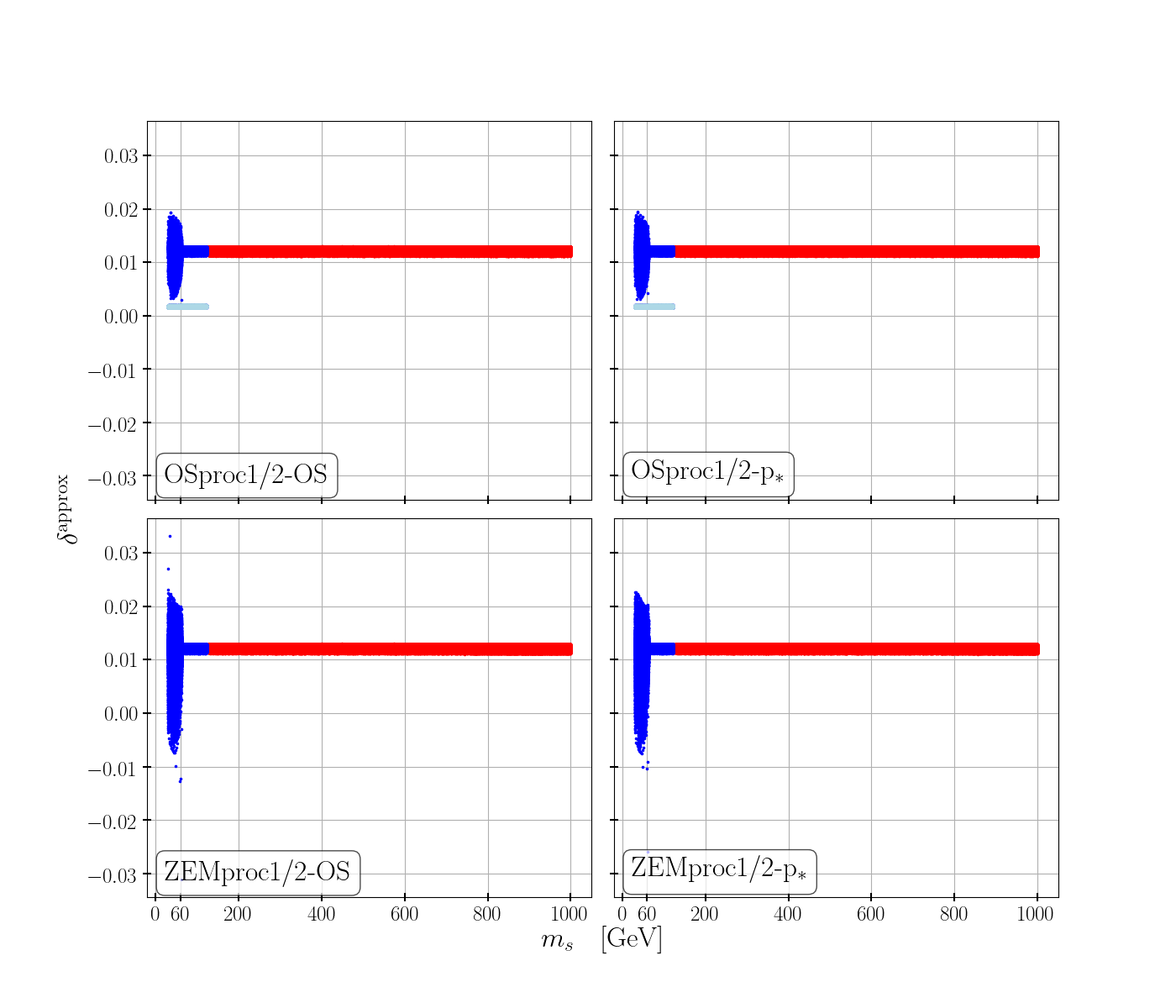
Figure 7: Relative uncertainty $\delta^{\text{approx}}$ in the EW NLO BR$(h_{125}\to AA)$ due to using the EW correction in the partial decay width for $h_{125}\to AA$ only, as a function of the mass $m_{S}$ of the non-SM-like Higgs boson for scenario I (red) and II (blue points) in the four possible different renormalization schemes.

6.5.2 Impact on Allowed Parameter Regions

In order to investigate the phenomenological impact of the EW corrections we generated two parameter samples: Sample 1 is the parameter sample which we also used in the previous sections. It is based on the check of the single- and di-Higgs constraints using the branching ratios at LO in the EW corrections. Sample 2 is the parameter sample, where we include the EW corrections in the branching ratios as defined in Eq. (31). As renormalization scheme, we use the ZEM scheme, more specifically ZEMproc2-OS, as it allows to use the largest amount of parameter scenarios. We do not apply any mass cuts or cuts on the couplings to suppress large NLO corrections. We only make sure to exclude parameter scenarios where the EW corrections lead to unphysical negative decay widths.

We then investigate if the allowed parameter regions of sample 2 change with respect to sample 1. We find that more points are rejected when we include the NLO corrections compared to the case where we only take LO decay widths (see also discussion below). Unfortunately, however, the shape of the allowed parameter regions overall did not change. The NLO corrections hence do not have a direct impact on the exclusion of certain parameter regions of our model yet. With increasing experimental precision in the future, it is evident, however, that higher-order EW corrections have to be considered.

6.6 Higgs Pair Production

Higgs pair production is one of the most prominent processes investigated at the LHC. Its measurement allows the extraction of the trilinear Higgs self-interaction [81] and thereby the ultimate experimental test of the Higgs mechanism [82, 83]. At the LHC, the dominant Higgs pair production process is gluon fusion into Higgs pairs [81, 84, 85] which at LO is mediated by heavy quark triangle and box diagrams [86, 87, 88]. The experiments search for Higgs pairs both in resonant and non-resonant Higgs pair production. The limits on the Higgs self-coupling between three SM-like Higgs bosons in terms of the SM trilinear Higgs coupling are at 95% CL $\kappa_{\lambda}\in[-0.4,6.3]$ given by ATLAS [89] and $\kappa_{\lambda}\in[-1.24,6.49]$ given by CMS [90]. After applying all constraints described in Sec. 5 we find for the still allowed $\kappa_{\lambda}$ values in the CxSM,

$$\begin{array}[]{ll}\mbox{Scenario I }(h_{1}\equiv h_{125}):&\kappa_{\lambda}\in[0.55,1.10]\\ \mbox{Scenario II }(h_{2}\equiv h_{125}):&\kappa_{\lambda}\in[0.15,1.21]\end{array}\;.$$ (52)

So there is still some room left to deviate from the SM value, values equal to zero are excluded, however. When compared to other models as e.g. those discussed in [63], we see that the trilinear self-coupling of the SM-like Higgs in the CxSM, when $h_{1}\equiv h_{125}$, is in general more constrained than in the CP-conserving (2HDM) and CP-violating 2-Higgs-Doublet Model (C2HDM), the next-to-2HDM (N2HDM) or the next-to-minimal supersymmetric extension (NMSSM) where for some of the models the coupling can still be zero and also take negative values. In case of scenario II, the lower limit is below the one in the (C)2HDM and the N2HDM. It is interesting to note, that in the case that we do not cut out degenerate Higgs scenarios with large mixing angles where the discovered Higgs signal is built up by two scalar resonances close to each other, larger deviations in the trilinear couplings would be possible, with negative or zero trilinear coupling values. After application of the NLO EW corrections and hence using the sample 2, we see that the Higgs self-couplings are not further constrained compared to sample 1.

While the range of allowed trilinear Higgs self-couplings is not sensitive yet to the EW corrections on the Higgs decays, the di-Higgs production cross sections are sensitive. More specifically, the maximum allowed di-Higgs cross section depends on whether or not EW corrections are included. When we use sample 1 where we calculate the resonant di-Higgs rate by multiplying the NNLO QCD $h_{2}$ production cross section obtained from SuShi with the LO branching ratio BR($h_{2}\to h_{1}h_{1}$) then the maximum allowed di-Higgs cross section is given by BP3, defined as

$$\begin{array}[]{llll}\lx@intercol\mbox{\text@underline{{\tt BP3}: Sample 1 - max di-Higgs at LO EW}}\hfil\lx@intercol\\ \mbox{Input parameters:}&m_{h_{1}}=125.09\mbox{ GeV }&m_{h_{2}}=260.96\mbox{ GeV }&m_{A}=257.36\mbox{ GeV }\\ &\alpha=-0.312&v_{S}=87.61\mbox{ GeV.}\end{array}$$ (56)

The SM-like di-Higgs production cross section, the trilinear ($\kappa_{h_{i}h_{j}h_{k}}$) and top-Yukawa couplings ($y_{t,h_{1/2}}$) normalized to the SM values are given by

$$\begin{array}[]{lll}\sigma_{h_{1}h_{1}}=585\mbox{ fb: }&\kappa_{h_{1}h_{1}h_{1}}=0.781&y_{t,h_{1}}=0.952\\ &\kappa_{h_{2}h_{1}h_{1}}=1.122&h_{t,h_{2}}=0.307\end{array}$$ (59)

For completeness, we also give the di-Higgs values for NLO branching ratios for the various renormalization schemes. The values in brackets are the consistently converted $v_{S}$ and $\alpha$ values. We have in the ZEMproc1-OS scheme $\sigma_{h_{1}h_{1}}=563.56$ fb (75.28 GeV, -0.312), in the ZEMproc1-$p_{\star}$ scheme $\sigma_{h_{1}h_{1}}=563.64$ fb (75.39 GeV, -0.312), in the ZEMproc2-OS scheme $\sigma_{h_{1}h_{1}}=603.94$ fb (87.61 GeV, -0.312), and in the ZEMproc2-$p_{\star}$ scheme $\sigma_{h_{1}h_{1}}=603.78$ fb (87.60 GeV, -0.312). For this parameter point, the maximum relative correction of the cross section is small with 3%, with the corresponding uncertainty on the NLO corrected cross section of 7% being larger.

If on the other hand, we take the parameter values of sample 2 where the di-Higgs constraints are applied to resonant $h_{1}h_{1}$ production computed with the NLO branching ratio of $h_{2}\to h_{1}h_{1}$, then we obtain, when we apply the ZEMproc2-OS scheme, the still allowed maximum cross section from benchmark point BP4, defined as

$$\begin{array}[]{llll}\lx@intercol\mbox{\text@underline{{\tt BP4}: Sample 2 - max di-Higgs at NLO EW (ZEMproc2-OS)}}\hfil\lx@intercol\\ \mbox{Input parameters:}&m_{h_{1}}=125.09\mbox{ GeV }&m_{h_{2}}=262.25\mbox{ GeV }&m_{A}=337.43\mbox{ GeV }\\ &\alpha=-0.317&v_{S}=101.03\mbox{ GeV,}\end{array}$$ (63)

with the following di-Higgs cross section and relevant coupling modifiers

$$\begin{array}[]{lll}\sigma_{h_{1}h_{1}}=582.84\mbox{ fb: }&\kappa_{h_{1}h_{1}h_{1}}=0.783&y_{t,h_{1}}=0.950\\ &\kappa_{h_{2}h_{1}h_{1}}=1.081&h_{t,h_{2}}=0.312\end{array}$$ (66)

The di-Higgs cross section changes to 577.61 fb if we multiply the SusHi $h_{2}$ production cross section with the LO branching ratio of the $h_{2}\to h_{1}h_{1}$ decay. As can be inferred from these values, the maximum allowed cross section barely varies from non-exclusion (BP3) to inclusion (BP4) of the EW corrections in the branching ratio of the di-Higgs decay. We also give the cross sections obtained for the other renormalization schemes. We have in the ZEMproc1-OS scheme $\sigma_{h_{1}h_{1}}=527.86$ fb (85.59 GeV, -0.317), in the ZEMproc1-$p_{\star}$ scheme $\sigma_{h_{1}h_{1}}=528.01$ fb (85.72 GeV, -0.318), and in the ZEMproc2-$p_{\star}$ scheme $\sigma_{h_{1}h_{1}}=582.63$ fb (101.02 GeV, -0.318). For this parameter point, the maximum relative correction of the cross section is small with -9%. The corresponding uncertainty on the NLO corrected cross section is again larger with 10%.

Comparing the results for BP3 and BP4, we remark that the NLO value in the ZEMproc2-OS scheme of BP3 exceeds the one of BP4, which is the reason why BP3 is excluded in sample 2 due to the resonant di-Higgs constraints. However, it should be noted that for these points the relative corrections are small and below the theory uncertainties. This is also reflected in the fact that the allowed trilinear values barely change independent if we include or not the EW corrections in the Higgs-to-Higgs decay branching ratio. Overall we find, when we apply the resonant di-Higgs constraints from the experimental searches, that less points are rejected when the NLO branching ratio BR($h_{2}\to h_{1}h_{1}$) is included instead of the LO one. This has to be taken with caution, however, due to remaining theory uncertainties. And we remind that we do not apply the resonant di-Higgs constraints when the narrow-width approximation is not justified any more. Since the total width can be smaller or larger depending on the parameter point and the inclusion or not of the EW corrections in the decay widths this of course also has an impact on the excluded region.

6.7 Points with Vanishing Coupling $\lambda_{h_{1}h_{1}h_{2}}$

The discussion so far has shown that the NLO corrections do not impact the shape of the parameter regions that are still allowed but they affect individual parameter points. We want to discuss now the interesting situation of parameter configurations where the trilinear coupling $\lambda_{h_{1}h_{1}h_{2}}$ is close to zero. Here, the impact of the NLO corrections could become important. We found that this is indeed the case. For some of these parameter points the NLO corrections to $h_{2}\to h_{1}h_{1}$ shifted the point above the allowed Higgs data constraints. As an example we look at the benchmark point BP5, defined as

$$\begin{array}[]{llll}\lx@intercol\mbox{\text@underline{{\tt BP5}: Scenario 2 - small $\lambda_{h_{1}h_{1}h_{2}}$}}\hfil\lx@intercol\\ \mbox{Input parameters:}&m_{h_{1}}=46.11\mbox{ GeV }&m_{h_{2}}=125.09\mbox{ GeV }&m_{A}=60.88\mbox{ GeV }\\ &\alpha=1.390&v_{S}=818.10\mbox{ GeV.}\end{array}$$ (70)

We are close to the case $\tan\alpha=v_{S}/v$ where the coupling $\lambda_{h_{1}h_{1}h_{2}}$ vanishes so that the partial decay width $\Gamma(h_{2}\to h_{1}h_{1})$ is small. The inclusion of the NLO corrections can considerably change this. And indeed we find, that the relative correction is (in the ZEMproc2-OS scheme)

$$\delta_{\text{EW}}(h_{2}\to h_{1}h_{1})=0.55\;.$$ (71)

This shift is so large that the parameter point is not allowed any more when NLO corrections are included.

7 Conclusions

In this paper we computed the EW corrections to the decay widths of the visible Higgs bosons of the CxSM, the SM extended by a complex singlet field. Applying two separate $\mathbb{Z}_{2}$ symmetries and requiring one VEV to be zero, the model contains one stable DM candidate. The EW corrections complete a previous computation of our group where the EW corrections to the Higgs decays into a DM pair were computed, by calculating the EW corrections to the decays into on-shell fermionic, massive gauge boson and Higgs pair final states. We do not compute corrections to off-shell decays nor to the loop-induced decays into gluon or photon pairs. We apply two different renormalization schemes for the renormalization of the mixing angle and four different schemes for the renormalization of the singlet VEV. The latter is renormalized process-dependent both on-shell and in the so-called ZEM scheme that we introduced in a previous calculation. The renormalization of the mixing angle is gauge-parameter independent by applying the alternative tadpole scheme and extracting the gauge-independent self-energies through the pinch technique. Our computation has been implemented in the code EWsHDECAY which has been publicly made available. The user has the options to choose between different renormalization schemes, including also the possibility to convert the input parameters, which has to be applied for a meaningful interpretation of the change of the renormalization scheme. For the numerical analysis we performed an extensive scan in the CxSM parameter space including theoretical and experimental constraints as well as DM constraints. We also considered the constraints from di-Higgs searches at the LHC. We found that our parameter points are able to saturate the DM relic density, and that direct search limits are already sensitive to parts of the model for parts of the DM mass region where the collider searches in invisible SM-like Higgs decays are not sensitive due to kinematic constraints.

The analysis of the impact of the relative EW corrections showed that they can be large in case of relatively large involved couplings, due to threshold effects or because the LO decay width is small. Here, the NLO width can become important and exclude parameter points that would be allowed at LO. For parameter configurations with exactly vanishing LO, and hence also, NLO width, we included the option to calculate the next-to-next-to-leading-order (NNLO) width. The applied formula is, however, only approximate when moving away from the exact zero LO value. If we exclude parameter configurations with large couplings or large threshold effects, the relative corrections are of typical EW size of up to 25%. The estimated theory uncertainty due to missing higher-order corrections based on the change of the renormalization scheme with converted input parameters is of a few per cent. The phenomenological impact of the computed EW corrections is that specific parameter points that are allowed at LO would be excluded at NLO. The overall distribution of the allowed parameter points, however, is not yet affected by the EW corrections. With increasing future precision in the experiments, this will change, however, and the here computed corrections provide an important contribution to reliably constrain the allowed parameter space of the model.

We also investigated the phenomenology of di-Higgs production. Our parameter scan revealed that deviations of the SM-like trilinear Higgs self-coupling from the SM value are still allowed. However, vanishing or negative trilinear coupling values are not allowed any more. The allowed range of the trilinear coupling barely changes when we include the NLO instead of the LO branching ratio in the Higgs-to-Higgs decay in resonant di-Higgs production and compare with the experimental results on resonant di-Higgs searches. For the investigated parameter points with maximum di-Higgs cross sections at LO, respectively at NLO, we found that the relative corrections on the di-Higgs cross sections are small and below the theory uncertainty. This picture may change, however, when the full EW corrections to the complete di-Higgs production cross section are considered.

Acknowledgments

RS and JV are supported by FCT under contracts UIDB/00618/2020, UIDP/00618/2020, PTDC/FIS-PAR/31000/2017, CERN/FISPAR /0002/2017, CERN/FIS-PAR/0014/2019. The work of FE and MM is supported by the BMBF-Project 05H21VKCCA.

References

- [1] ATLAS collaboration, G. Aad et al., Observation of a new particle in the search for the Standard Model Higgs boson with the ATLAS detector at the LHC, Phys. Lett. B 716 (2012) 1–29, [1207.7214].
- [2] CMS collaboration, S. Chatrchyan et al., Observation of a New Boson at a Mass of 125 GeV with the CMS Experiment at the LHC, Phys. Lett. B 716 (2012) 30–61, [1207.7235].
- [3] F. Egle, M. Mühlleitner, R. Santos and J. a. Viana, One-loop corrections to the Higgs boson invisible decay in a complex singlet extension of the SM, Phys. Rev. D 106 (2022) 095030, [2202.04035].
- [4] ATLAS collaboration, M. Aaboud et al., Combination of searches for invisible Higgs boson decays with the ATLAS experiment, Phys. Rev. Lett. 122 (2019) 231801, [1904.05105].
- [5] R. Costa, M. Mühlleitner, M. O. P. Sampaio and R. Santos, Singlet Extensions of the Standard Model at LHC Run 2: Benchmarks and Comparison with the NMSSM, JHEP 06 (2016) 034, [1512.05355].
- [6] A. Djouadi, J. Kalinowski and M. Spira, Hdecay: a program for higgs boson decays in the standard model and its supersymmetric extension, Computer Physics Communications 108 (Jan, 1998) 56–74.
- [7] A. Djouadi, J. Kalinowski, M. Mühlleitner and M. Spira, Hdecay: Twenty++ years after, Computer Physics Communications 238 (May, 2019) 214–231.
- [8] sHDECAY collaboration, R. Costa, M. Mühlleitner, M. Sampaio and R. Santos, Webpage for download of sHDECAY, https://www.itp.kit.edu/ maggie/sHDECAY/ .
- [9] M. Krause, R. Lorenz, M. Muhlleitner, R. Santos and H. Ziesche, Gauge-independent Renormalization of the 2-Higgs-Doublet Model, JHEP 09 (2016) 143, [1605.04853].
- [10] M. Krause, M. Muhlleitner, R. Santos and H. Ziesche, Higgs-to-Higgs boson decays in a 2HDM at next-to-leading order, Phys. Rev. D 95 (2017) 075019, [1609.04185].
- [11] M. Krause, M. Mühlleitner and M. Spira, 2HDECAY —A program for the calculation of electroweak one-loop corrections to Higgs decays in the Two-Higgs-Doublet Model including state-of-the-art QCD corrections, Comput. Phys. Commun. 246 (2020) 106852, [1810.00768].
- [12] M. Krause and M. Mühlleitner, Impact of Electroweak Corrections on Neutral Higgs Boson Decays in Extended Higgs Sectors, JHEP 04 (2020) 083, [1912.03948].
- [13] M. Krause, D. Lopez-Val, M. Muhlleitner and R. Santos, Gauge-independent Renormalization of the N2HDM, JHEP 12 (2017) 077, [1708.01578].
- [14] M. Krause and M. Mühlleitner, ewN2HDECAY - A program for the Calculation of Electroweak One-Loop Corrections to Higgs Decays in the Next-to-Minimal Two-Higgs-Doublet Model Including State-of-the-Art QCD Corrections, 1904.02103.
- [15] A. Denner, L. Jenniches, J.-N. Lang and C. Sturm, Gauge-independent renormalization in the 2HDM, JHEP 09 (2016) 115, [1607.07352].
- [16] L. Altenkamp, S. Dittmaier and H. Rzehak, Renormalization schemes for the Two-Higgs-Doublet Model and applications to h WW/ZZ 4 fermions, JHEP 09 (2017) 134, [1704.02645].
- [17] L. Altenkamp, S. Dittmaier and H. Rzehak, Precision calculations for fermions in the Two-Higgs-Doublet Model with Prophecy4f, JHEP 03 (2018) 110, [1710.07598].
- [18] A. Denner, S. Dittmaier and J.-N. Lang, Renormalization of mixing angles, Journal of High Energy Physics 2018 (Nov, 2018) 104.
- [19] M. Fox, W. Grimus and M. Löschner, Renormalization and radiative corrections to masses in a general Yukawa model, Int. J. Mod. Phys. A 33 (2018) 1850019, [1705.09589].
- [20] W. Grimus and M. Löschner, Renormalization of the multi-Higgs-doublet Standard Model and one-loop lepton mass corrections, JHEP 11 (2018) 087, [1807.00725].
- [21] J. Fleischer and F. Jegerlehner, Radiative Corrections to Higgs Decays in the Extended Weinberg-Salam Model, Phys. Rev. D 23 (1981) 2001–2026.
- [22] A. Pilaftsis, Resonant CP violation induced by particle mixing in transition amplitudes, Nucl. Phys. B 504 (1997) 61–107, [hep-ph/9702393].
- [23] S. Kanemura, Y. Okada, E. Senaha and C. P. Yuan, Higgs coupling constants as a probe of new physics, Phys. Rev. D 70 (2004) 115002, [hep-ph/0408364].
- [24] J. M. Cornwall and J. Papavassiliou, Gauge invariant three gluon vertex in qcd, Phys. Rev. D40 (1989) 3474.
- [25] J. Papavassiliou, Gauge independent transverse and longitudinal self-energies and vertices via the pinch technique, Phys. Rev. D50 (1994) 5958–5970, [hep-ph/9406258].
- [26] D. Azevedo, P. Gabriel, M. Muhlleitner, K. Sakurai and R. Santos, One-loop corrections to the Higgs boson invisible decay in the dark doublet phase of the N2HDM, JHEP 10 (2021) 044, [2104.03184].
- [27] A. Bredenstein, A. Denner, S. Dittmaier and M. M. Weber, Precise predictions for the Higgs-boson decay H — WW/ZZ — 4 leptons, Phys. Rev. D 74 (2006) 013004, [hep-ph/0604011].
- [28] J. Kublbeck, M. Bohm and A. Denner, Feyn Arts: Computer Algebraic Generation of Feynman Graphs and Amplitudes, Comput. Phys. Commun. 60 (1990) 165–180.
- [29] T. Hahn, Generating Feynman diagrams and amplitudes with FeynArts 3, Comput. Phys. Commun. 140 (2001) 418–431, [hep-ph/0012260].
- [30] R. Mertig, M. Bohm and A. Denner, FEYN CALC: Computer algebraic calculation of Feynman amplitudes, Comput. Phys. Commun. 64 (1991) 345–359.
- [31] V. Shtabovenko, R. Mertig and F. Orellana, New Developments in FeynCalc 9.0, Comput. Phys. Commun. 207 (2016) 432–444, [1601.01167].
- [32] T. Hahn and M. Perez-Victoria, Automatized one loop calculations in four-dimensions and D-dimensions, Comput. Phys. Commun. 118 (1999) 153–165, [hep-ph/9807565].
- [33] G. J. van Oldenborgh and J. A. M. Vermaseren, New Algorithms for One Loop Integrals, Z. Phys. C 46 (1990) 425–438.
- [34] F. Staub, From Superpotential to Model Files for FeynArts and CalcHep/CompHep, Comput. Phys. Commun. 181 (2010) 1077–1086, [0909.2863].
- [35] F. Staub, Automatic Calculation of supersymmetric Renormalization Group Equations and Self Energies, Comput. Phys. Commun. 182 (2011) 808–833, [1002.0840].
- [36] F. Staub, SARAH 3.2: Dirac Gauginos, UFO output, and more, Comput. Phys. Commun. 184 (2013) 1792–1809, [1207.0906].
- [37] F. Staub, SARAH 4 : A tool for (not only SUSY) model builders, Comput. Phys. Commun. 185 (2014) 1773–1790, [1309.7223].
- [38] F. Staub, Exploring new models in all detail with SARAH, Adv. High Energy Phys. 2015 (2015) 840780, [1503.04200].
- [39] N. D. Christensen and C. Duhr, FeynRules - Feynman rules made easy, Comput. Phys. Commun. 180 (2009) 1614–1641, [0806.4194].
- [40] C. Degrande, C. Duhr, B. Fuks, D. Grellscheid, O. Mattelaer and T. Reiter, UFO - The Universal FeynRules Output, Comput. Phys. Commun. 183 (2012) 1201–1214, [1108.2040].
- [41] A. Alloul, N. D. Christensen, C. Degrande, C. Duhr and B. Fuks, FeynRules 2.0 - A complete toolbox for tree-level phenomenology, Comput. Phys. Commun. 185 (2014) 2250–2300, [1310.1921].
- [42] R. Coimbra, M. O. P. Sampaio and R. Santos, ScannerS: Constraining the phase diagram of a complex scalar singlet at the LHC, Eur. Phys. J. C 73 (2013) 2428, [1301.2599].
- [43] M. Mühlleitner, M. O. P. Sampaio, R. Santos and J. Wittbrodt, ScannerS: Parameter Scans in Extended Scalar Sectors, 2007.02985.
- [44] LHC Higgs Cross Section Working Group, LHC Twiki page.
- [45] Particle Data Group collaboration, P. Zyla et al., Review of Particle Physics, PTEP 2020 (2020) 083C01.
- [46] B. W. Lee, C. Quigg and H. B. Thacker, Weak Interactions at Very High-Energies: The Role of the Higgs Boson Mass, Phys. Rev. D 16 (1977) 1519.
- [47] M. E. Peskin and T. Takeuchi, Estimation of oblique electroweak corrections, Phys. Rev. D 46 (07, 1992) 381–409.
- [48] P. Bechtle, S. Heinemeyer, O. Stål, T. Stefaniak and G. Weiglein, : Confronting arbitrary Higgs sectors with measurements at the Tevatron and the LHC, Eur. Phys. J. C 74 (2014) 2711, [1305.1933].
- [49] P. Bechtle, S. Heinemeyer, T. Klingl, T. Stefaniak, G. Weiglein and J. Wittbrodt, HiggsSignals-2: Probing new physics with precision Higgs measurements in the LHC 13 TeV era, Eur. Phys. J. C 81 (2021) 145, [2012.09197].
- [50] P. Bechtle, O. Brein, S. Heinemeyer, G. Weiglein and K. E. Williams, HiggsBounds: Confronting Arbitrary Higgs Sectors with Exclusion Bounds from LEP and the Tevatron, Comput. Phys. Commun. 181 (2010) 138–167, [0811.4169].
- [51] P. Bechtle, D. Dercks, S. Heinemeyer, T. Klingl, T. Stefaniak, G. Weiglein et al., HiggsBounds-5: Testing Higgs Sectors in the LHC 13 TeV Era, 2006.06007.
- [52] G. Belanger, F. Boudjema, A. Pukhov and A. Semenov, MicrOMEGAs 2.0: A Program to calculate the relic density of dark matter in a generic model, Comput. Phys. Commun. 176 (2007) 367–382, [hep-ph/0607059].
- [53] C. Gross, O. Lebedev and T. Toma, Cancellation Mechanism for Dark-Matter–Nucleon Interaction, Phys. Rev. Lett. 119 (2017) 191801, [1708.02253].
- [54] D. Azevedo, M. Duch, B. Grzadkowski, D. Huang, M. Iglicki and R. Santos, Testing scalar versus vector dark matter, Phys. Rev. D 99 (2019) 015017, [1808.01598].
- [55] D. Azevedo, M. Duch, B. Grzadkowski, D. Huang, M. Iglicki and R. Santos, One-loop contribution to dark-matter-nucleon scattering in the pseudo-scalar dark matter model, JHEP 01 (2019) 138, [1810.06105].
- [56] S. Glaus, M. Mühlleitner, J. Müller, S. Patel, T. Römer and R. Santos, Electroweak Corrections in a Pseudo-Nambu Goldstone Dark Matter Model Revisited, JHEP 12 (2020) 034, [2008.12985].
- [57] XENON collaboration, E. Aprile et al., Dark Matter Search Results from a One Ton-Year Exposure of XENON1T, Phys. Rev. Lett. 121 (2018) 111302, [1805.12562].
- [58] PandaX-4T collaboration, Y. Meng et al., Dark Matter Search Results from the PandaX-4T Commissioning Run, Phys. Rev. Lett. 127 (2021) 261802, [2107.13438].
- [59] J. Aalbers et al., First dark matter search results from the lux-zeplin (lz) experiment, 2022. 10.48550/ARXIV.2207.03764.
- [60] P. Basler and M. Mühlleitner, BSMPT (Beyond the Standard Model Phase Transitions): A tool for the electroweak phase transition in extended Higgs sectors, Comput. Phys. Commun. 237 (2019) 62–85, [1803.02846].
- [61] P. Basler, M. Mühlleitner and J. Müller, BSMPT v2 a tool for the electroweak phase transition and the baryon asymmetry of the universe in extended Higgs Sectors, Comput. Phys. Commun. 269 (2021) 108124, [2007.01725].
- [62] A. D. Sakharov, Violation of CP Invariance, c Asymmetry, and Baryon Asymmetry of the Universe, Pisma Zh. Eksp. Teor. Fiz. 5 (1967) 32–35.
- [63] H. Abouabid, A. Arhrib, D. Azevedo, J. E. Falaki, P. M. Ferreira, M. Mühlleitner et al., Benchmarking di-Higgs production in various extended Higgs sector models, JHEP 09 (2022) 011, [2112.12515].
- [64] R. V. Harlander, S. Liebler and H. Mantler, SusHi: A program for the calculation of Higgs production in gluon fusion and bottom-quark annihilation in the Standard Model and the MSSM, Comput. Phys. Commun. 184 (2013) 1605–1617, [1212.3249].
- [65] S. Liebler, Neutral Higgs production at proton colliders in the CP-conserving NMSSM, Eur. Phys. J. C 75 (2015) 210, [1502.07972].
- [66] R. V. Harlander, S. Liebler and H. Mantler, SusHi Bento: Beyond NNLO and the heavy-top limit, Comput. Phys. Commun. 212 (2017) 239–257, [1605.03190].
- [67] ATLAS collaboration, M. Aaboud et al., Search for pair production of Higgs bosons in the final state using proton-proton collisions at TeV with the ATLAS detector, JHEP 01 (2019) 030, [1804.06174].
- [68] ATLAS Collaboration collaboration, Search for resonant pair production of Higgs bosons in the final state using collisions at = 13 TeV with the ATLAS detector, , CERN, Geneva, Aug, 2021.
- [69] CMS collaboration, Search for resonant Higgs boson pair production in four b quark final state using large-area jets in proton-proton collisions at , .
- [70] ATLAS collaboration, M. Aaboud et al., Search for resonant and non-resonant Higgs boson pair production in the decay channel in collisions at TeV with the ATLAS detector, Phys. Rev. Lett. 121 (2018) 191801, [1808.00336].
- [71] ATLAS collaboration, G. Aad et al., Reconstruction and identification of boosted di- systems in a search for Higgs boson pairs using 13 TeV proton-proton collision data in ATLAS, JHEP 11 (2020) 163, [2007.14811].
- [72] ATLAS Collaboration collaboration, Search for resonant and non-resonant Higgs boson pair production in the decay channel using 13 TeV collision data from the ATLAS detector, , CERN, Geneva, Jul, 2021.
- [73] ATLAS collaboration, M. Aaboud et al., Search for Higgs boson pair production in the final state with 13 TeV collision data collected by the ATLAS experiment, JHEP 11 (2018) 040, [1807.04873].
- [74] ATLAS Collaboration collaboration, Search for Higgs boson pair production in the two bottom quarks plus two photons final state in collisions at TeV with the ATLAS detector, , CERN, Geneva, Mar, 2021.
- [75] ATLAS collaboration, M. Aaboud et al., Search for Higgs boson pair production in the decay mode at TeV with the ATLAS detector, JHEP 04 (2019) 092, [1811.04671].
- [76] CMS collaboration, A. M. Sirunyan et al., Search for resonant pair production of Higgs bosons in the channel in proton-proton collisions at 13 TeV, Phys. Rev. D 102 (2020) 032003, [2006.06391].
- [77] ATLAS collaboration, M. Aaboud et al., Search for Higgs boson pair production in the channel using collision data recorded at TeV with the ATLAS detector, Eur. Phys. J. C 78 (2018) 1007, [1807.08567].
- [78] ATLAS collaboration, M. Aaboud et al., Search for Higgs boson pair production in the decay channel using ATLAS data recorded at TeV, JHEP 05 (2019) 124, [1811.11028].
- [79] Planck collaboration, N. Aghanim et al., Planck 2018 results. VI. Cosmological parameters, Astron. Astrophys. 641 (2020) A6, [1807.06209].
- [80] G. Passarino and M. J. G. Veltman, One Loop Corrections for e+ e- Annihilation Into mu+ mu- in the Weinberg Model, Nucl. Phys. B 160 (1979) 151–207.
- [81] J. Alison et al., Higgs boson potential at colliders: Status and perspectives, Rev. Phys. 5 (2020) 100045, [1910.00012].
- [82] A. Djouadi, W. Kilian, M. Muhlleitner and P. M. Zerwas, Testing Higgs selfcouplings at e+ e- linear colliders, Eur. Phys. J. C 10 (1999) 27–43, [hep-ph/9903229].
- [83] A. Djouadi, W. Kilian, M. Mühlleitner and P. M. Zerwas, Production of neutral Higgs boson pairs at LHC, Eur. Phys. J. C10 (1999) 45–49, [hep-ph/9904287].
- [84] J. Baglio, A. Djouadi, R. Gröber, M. M. Mühlleitner, J. Quevillon and M. Spira, The measurement of the Higgs self-coupling at the LHC: theoretical status, JHEP 04 (2013) 151, [1212.5581].
- [85] LHC Higgs Cross Section Working Group collaboration, D. de Florian et al., Handbook of LHC Higgs Cross Sections: 4. Deciphering the Nature of the Higgs Sector, 1610.07922.
- [86] E. W. N. Glover and J. J. van der Bij, HIGGS BOSON PAIR PRODUCTION VIA GLUON FUSION, Nucl. Phys. B309 (1988) 282–294.
- [87] D. A. Dicus, C. Kao and S. S. D. Willenbrock, Higgs Boson Pair Production From Gluon Fusion, Phys. Lett. B 203 (1988) 457–461.
- [88] T. Plehn, M. Spira and P. M. Zerwas, Pair production of neutral Higgs particles in gluon-gluon collisions, Nucl. Phys. B479 (1996) 46–64, [hep-ph/9603205].
- [89] ATLAS collaboration, Constraining the Higgs boson self-coupling from single- and double-Higgs production with the ATLAS detector using collisions at TeV, 2211.01216.
- [90] CMS collaboration, A. Tumasyan et al., A portrait of the Higgs boson by the CMS experiment ten years after the discovery, Nature 607 (2022) 60–68, [2207.00043].