(Technical Report)
PANE-GNN: Unifying Positive and Negative Edges
in Graph Neural Networks for Recommendation

Abstract.

Recommender systems play a crucial role in addressing the issue of information overload by delivering personalized recommendations to users. In recent years, there has been a growing interest in leveraging graph neural networks (GNNs) for recommender systems, capitalizing on advancements in graph representation learning. These GNN-based models primarily focus on analyzing users’ positive feedback while overlooking the valuable insights provided by their negative feedback. In this paper, we propose PANE-GNN, an innovative recommendation model that unifies Positive And Negative Edges in Graph Neural Networks for recommendation. By incorporating user preferences and dispreferences, our approach enhances the capability of recommender systems to offer personalized suggestions. PANE-GNN first partitions the raw rating graph into two distinct bipartite graphs based on positive and negative feedback. Subsequently, we employ two separate embeddings, the interest embedding and the disinterest embedding, to capture users’ likes and dislikes, respectively. To facilitate effective information propagation, we design distinct message-passing mechanisms for positive and negative feedback. Furthermore, we introduce a distortion to the negative graph, which exclusively consists of negative feedback edges, for contrastive training. This distortion plays a crucial role in effectively denoising the negative feedback. The experimental results provide compelling evidence that PANE-GNN surpasses the existing state-of-the-art benchmark methods across four real-world datasets. These datasets include three commonly used recommender system datasets and one open-source short video recommendation dataset.

1. Introduction

Recommender systems have garnered significant attention as a prominent research field, offering solutions in information filtering by predicting users’ item ratings or preferences (Hwang and Chae, 2022a, b; Kim et al., 2022; Oh et al., 2022; Rendle et al., 2009; He et al., 2017). The versatility of recommender systems is evident through their widespread adoption across diverse domains, establishing their importance in recent years. Notably, recommender systems have found practical applications in domains such as movies (Darban and Valipour, 2022; Ning et al., 2022), news (Zhang et al., 2022; Alshehri and Zhang, 2022), e-commerce items (Qin et al., 2022; Kim et al., 2022), and short videos (Gong et al., 2022; Yu et al., 2022a). Given the multitude of domains and the increasing reliance on these systems, the development of recommender systems has emerged as a critical concern within the field of computer science (Wu et al., 2022a; Zheng et al., 2023; Wu et al., 2023).

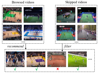
The fundamental structure of recommender systems’ user-item interaction graph can be represented as a signed bipartite graph, encompassing both positive and negative feedback from users. Positive feedback indicates user interest, while negative feedback denotes disinterest or dissatisfaction. Major platforms such as YouTube and Amazon offer mechanisms for users to express their preferences or assign ratings to items, reflecting these feedback categories. The incorporation of negative feedback assumes significance in cases where positive feedback signals are absent, serving as a critical means to prevent irrelevant or unnecessary recommendations to users. Figure 1 visually demonstrates the integration of positive and negative feedback, highlighting its potential for accurate recommendation outcomes.

Observation 1: Existing graph neural network (GNN) paradigms for recommendations fail to effectively incorporate negative feedback information, particularly in the context of message passing (Liu et al., 2022; Yu et al., 2022b; Pang et al., 2022; He et al., 2020; Seo et al., 2022). This limitation hampers the comprehensive utilization of valuable user feedback in recommender systems.

Figure 1. An example of video recommendation from YouTube. The integration of positive and negative feedback plays a pivotal role in achieving accurate recommendation outcomes. In this example, the user prefers team sports while showing no interest in single-player sports.

(a) Precision results.

(b) Recall results.

(c) nDCG results.

Figure 2. Comparison of single-relational (NGCF) and multi-relational (GHCF) recommendation models on the ML-1M dataset.

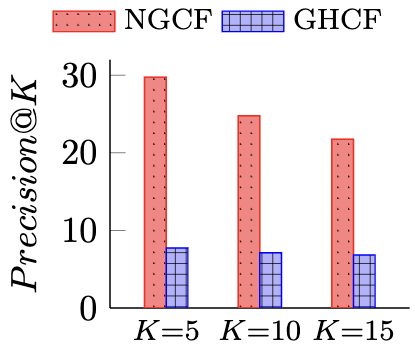
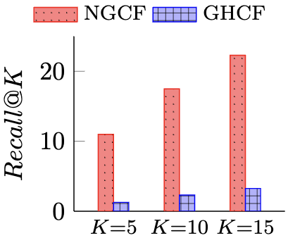
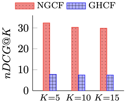
Observation 2: While incorporating negative feedback through a multiple-behavioral graph seems like a natural approach, our experiments with the state-of-the-art method GHCF (Chen et al., 2021) (shown in Figure 2) reveal a decrease in performance compared to NGCF that does not utilize negative feedback. It suggests that directly incorporating negative feedback may not always yield benefits.

Challenges. The aforementioned observations underscore the challenge of developing effective algorithms that can effectively incorporate negative feedback into recommender systems. The underutilization of negative feedback in current approaches motivates us to explore the usage of negative feedback through GNNs in order to enhance the quality of recommendations. However, learning high-order structural information from a signed bipartite graph faces difficulties due to the limitations of the network homophily assumption and the balance theory assumption. The network homophily assumption posits that similar nodes are more likely to connect to each other than dissimilar nodes. Many GNN models (Wang et al., 2019; Chen et al., 2020; He et al., 2020) adopt a message-passing mechanism that aggregates information from local neighbors to update the embedding of the anchor node based on this assumption. However, homophily is not applicable in signed graphs where dissimilar nodes are connected by negative edges. The balance theory assumption implies that “the friend of my friend is my friend”, “the enemy of my friend is my enemy”, and “the enemy of my enemy is my friend”. Existing methods for signed unipartite graphs (Derr et al., 2018; Yoo et al., 2022; Huang et al., 2021b) leverage this assumption to aggregate and propagate information across layers. However, the balance theory assumption does not match with the signed bipartite graph in recommender systems (Huang et al., 2021a; Xu et al., 2022, 2021). In real-world recommendation scenarios, users typically possess diverse interests rather than unique interests. Consequently, the fundamental idea of “the enemy of my enemy is my friend” (i.e., “two items disliked by the same user are similar”) in the balance theory assumption does not accurately capture the complexity of real-world situations. These limitations necessitate the development of novel approaches to effectively leverage negative feedback in recommender systems, accounting for the unique characteristics of signed bipartite graphs and the diverse interests of users in real-world settings.

Our idea. The key idea revolves around utilizing high-order structural information from both the positive graph (i.e., user-item interaction graph containing only positive feedback edges) and the negative graph (i.e., user-item interaction graph containing only negative feedback edges) simultaneously. To enhance recommendations by incorporating negative feedback, this paper presents a novel recommendation model called PANE-GNN (unifying Positive And Negative Edges in Graph Neural Networks for recommendation). In this model, each user or item is assigned two embeddings, i.e., interest embedding and disinterest embedding, to capture the user’s interests and disinterests, respectively. Taking into account the network homophily assumption, we devise two message-passing mechanisms for the positive graph and the negative graph. On the positive graph, interest embeddings are propagated and updated, capturing the user’s interests. On the other hand, on the negative graph, disinterest embeddings are propagated and updated, capturing the user’s disinterests or items they explicitly dislike. Furthermore, to generate robust embeddings that remain invariant to graph perturbations, we utilize graph contrastive learning on the negative graph and its perturbed version. This approach enhances the model’s ability to capture relevant patterns in the presence of graph noise.

The main three contributions of this work are as follows:

• We propose a novel GNN-based recommendation model called PANE-GNN. The model performs message passing on both the positive graph and the negative graph to effectively incorporate positive and negative feedback (Section 3.2.1).

• We design contrastive learning on the negative graph (Section 3.2.2), a new ranking method with a disinterest-score filter (Section 3.2.3), and a dual feedback-aware Bayesian personalized ranking loss (Section 3.3), all of which improve recommendation accuracy through the integration of positive and negative feedback signals.

• The proposed PANE-GNN is extensively evaluated on four real-world datasets (Section 4). The experimental results demonstrate that PANE-GNN outperforms state-of-the-art GNN-based recommendation methods.

2. Related Work

We provide a review of existing work about 1) recommender systems based on GNNs, and 2) graph neural networks on signed graphs.

2.1. Recommender Systems based on GNNs

Recently, GNNs have become the new state-of-the-art approach in many recommendation problems (Gao et al., 2022b; Wu et al., 2022b). The main advantage of using GNNs for recommender systems is that it can capture higher-order structural information in the observed data. Based on the message-passing architecture of GNNs, NGCF (Wang et al., 2019) adopts the Hadamard product between user embedding and item embedding to promote passing more messages from similar items to users. Considering that nonlinear activation contributes little to the recommendation performance, LR-GCCF (Chen et al., 2020) removes non-linearities from the original graph convolutional network (GCN) model (Kipf and Welling, 2017) and adds a residual network structure on it to alleviate the over-smoothing problem in the graph convolution aggregation. Likewise, LightGCN (He et al., 2020) removes both feature transformation and nonlinear activation and only retains neighborhood aggregation for collaborative filtering. The simplified model has higher computational efficiency and is much easier to implement and train.

Our proposed method differs from the above methods in that we consider the negative feedback information in the observed data and devise a novel message-passing process that takes into account both positive and negative feedback.

2.2. Graph Neural Networks on Signed Graphs

Most of the previous work focus on building GNNs for unsigned graphs where there are only positive edges. Currently, signed graphs where each edge has a positive or negative sign, have become increasingly ubiquitous in the real world. For example, the users in a social network may hold common or opposite political views. Since the network homophily assumption is the theoretical basis of the message-passing mechanism in GNNs, those unsigned GNNs cannot be applied to signed graphs directly. As a pioneering work of signed GNNs, SGCN (Derr et al., 2018) assigns balanced embedding and unbalanced embedding for each node and propagates the two embeddings in the signed graph based on balance theory. Furtherly, SNEA (Li et al., 2020) optimizes the message-passing process in SGCN by assigning different importance coefficients to each node pair connected with different edges. Inspired by adversarial learning, ASiNE (Lee et al., 2020) plays a minimax game in the positive graph and negative graph by leveraging a generator and a discriminator for positive edges and negative edges in a signed graph, respectively. SiReN (Seo et al., 2022) generates positive embeddings and negative embeddings for each node in a signed graph via a GNN model and a multilayer perceptron (MLP) model, respectively. Then SiReN adopts an attention layer to integrate the two embeddings into the final embeddings.

Unlike the existing methods based on the balance theory assumption, which may not be directly applicable to the signed bipartite graph in recommender systems, the proposed method in this work takes a different approach. It splits the raw rating graph into two distinct graphs and emphasizes the propagation of information within each graph based on the type of edges.

3. Method

In this section, we introduce the notations used in the paper, present the architecture of PANE-GNN, and describe its optimization objective.

3.1. Notations

In the given raw rating graph $\mathcal{G}=(\mathcal{U},\mathcal{I},\mathcal{E})$, where $\mathcal{U}$ represents the set of users, $\mathcal{I}$ represents the set of items, and $\mathcal{E}$ represents the set of edges, we split the graph into two edge-disjoint graphs: the positive graph $\mathcal{G}{p}=(\mathcal{U},\mathcal{I},\mathcal{E}{p})$ and the negative graph $\mathcal{G}{n}=(\mathcal{U},\mathcal{I},\mathcal{E}{n})$. Here, $\mathcal{E}{p}$ represents the edges corresponding to positive ratings, and $\mathcal{E}{n}$ represents the edges corresponding to negative ratings. The union of $\mathcal{E}{p}$ and $\mathcal{E}{n}$ gives the set of all edges $\mathcal{E}$. In the positive graph $\mathcal{G}{p}$, we aim to learn the interest embeddings for users and items, denoted as $\mathbf{z}_{u}$ and $\mathbf{z}_{i}$, respectively. These embeddings capture the relationship between liking and being liked. In contrast, in the negative graph $\mathcal{G}{n}$, we focus on learning the disinterest embeddings for users and items, represented as $\mathbf{v}_{u}$ and $\mathbf{v}_{i}$, respectively. These embeddings capture the relationship between disliking and being disliked. For a comprehensive overview of the notations used in this paper, please refer to Table 1.

Table 1. Frequently used notations in this paper.

Notation	Description
$\mathcal{U}$	Set of users.
$\mathcal{I}$	Set of items.
$\mathcal{E}_{p}$	Set of positive edges.
$\mathcal{E}_{n}$	Set of negative edges.
$\mathcal{E}=\mathcal{E}_{p}\cup\mathcal{E}_{n}$	Set of all edges.
$\mathcal{G}{=}(\mathcal{U},\mathcal{I},\mathcal{E})$	Raw rating graph.
$\mathcal{G}_{p}{=}(\mathcal{U},\mathcal{I},\mathcal{E}_{p})$	Positive graph.
$\mathcal{G}_{n}{=}(\mathcal{U},\mathcal{I},\mathcal{E}_{n})$	Negative graph.
$\mathcal{G}_{d}{=}(\mathcal{U},\mathcal{I},\mathcal{E}_{d})$	Distorted graph from $\mathcal{G}_{n}$.
$N=|\mathcal{U}{\cup}\mathcal{I}|$	Number of all nodes in $\mathcal{G}$.
$\mathbf{A}_{p},\mathbf{A}_{n},\mathbf{A}_{d}{\in}\mathbb{R}^{N{\times}N}$	Adjacency matrices of $\mathcal{G}_{p}$, $\mathcal{G}_{n}$, & $\mathcal{G}_{d}$.
$\mathcal{N}_{p}(u),\mathcal{N}_{n}(u),\mathcal{N}_{d}(u)$	Neighbor sets of user $u$ in $\mathcal{G}_{p}$, $\mathcal{G}_{n}$, & $\mathcal{G}_{d}$.
$\mathcal{N}_{p}(i),\mathcal{N}_{n}(i),\mathcal{N}_{d}(i)$	Neighbor sets of item $i$ in $\mathcal{G}_{p}$, $\mathcal{G}_{n}$, & $\mathcal{G}_{d}$.
$\mathbf{Z}{\in}\mathbb{R}^{N\times H}$	Interest embedding matrix.
$\mathbf{V}{\in}\mathbb{R}^{N\times H}$	Disinterest embedding matrix.
$\mathbf{z}_{u},\mathbf{z}_{i}{\in}\mathbb{R}^{H}$	Interest embeddings on $\mathcal{G}_{p}$.
$\mathbf{v}_{u},\mathbf{v}_{i}{\in}\mathbb{R}^{H}$	Disinterest embeddings on $\mathcal{G}_{n}$.
$\tilde{\mathbf{v}}_{u},\tilde{\mathbf{v}}_{i}{\in}\mathbb{R}^{H}$	Disinterest embeddings on $\mathcal{G}_{d}$.
$H$	Embedding size.
$K$	Layer number of graph neural networks.
$p$	Probability of edge removing.
$b$	Feedback-aware coefficient.
$\delta$	Filtering threshold.
$\lambda_{1}$	Contrastive learning coefficient.
$\lambda_{2}$	L2 regularization coefficient.
$\tau$	Temperature coefficient.

Figure 3. The architecture of PANE-GNN. In model training, PANE-GNN performs message passing on both $\mathcal{G}_{p}$ and $\mathcal{G}_{n}$ and contrastive learning on $\mathcal{G}_{n}$ to generate interest embedding $\mathbf{Z}$ and disinterest embedding $\mathbf{V}$. In model prediction, PANE-GNN recommends a sequence of items to each user based on a ranking method with a disinterest-score filter.

3.2. Model architecture

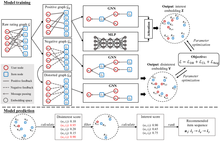
The architecture of the PANE-GNN model is depicted in Figure 3. It consists of three key technical designs: message passing on the positive graph $\mathcal{G}{p}$ and the negative graph $\mathcal{G}{n}$, contrastive learning on the negative graph $\mathcal{G}_{n}$, and ranking with a disinterest-score filter. In the message passing stage, information propagation takes place on both $\mathcal{G}{p}$ and $\mathcal{G}{n}$. This solution allows the model to leverage the structural information present in both graphs to enhance the representation learning process. The contrastive learning stage focuses on the negative graph $\mathcal{G}_{n}$. By employing contrastive learning, the model denoises the negative feedback and generates robust embeddings that remain invariant to graph perturbations. Finally, the ranking method with a disinterest-score filter is applied to generate the final recommendations. This method incorporates the learned embeddings from both the positive and negative graphs to rank the items and filter out items that do not align with the user’s interests.

3.2.1. Message passing on $\mathcal{G}_{p}$ and $\mathcal{G}_{n}$

In contrast to prior work that primarily focuses on message passing on the positive graph $\mathcal{G}{p}$, PANE-GNN takes into account the high-order structural information in the negative graph $\mathcal{G}{n}$ as well. In PANE-GNN, we introduce two types of embeddings: interest embeddings and disinterest embeddings. These embeddings capture the relationships between liking and being liked, as well as disliking and being disliked, respectively, for each user or item. To effectively aggregate and propagate these embeddings, PANE-GNN utilizes a technique called light graph convolution (LGC) (He et al., 2020), which allows the embeddings to be updated and combined within the respective graph structures. In the message passing process on the positive graph $\mathcal{G}_{p}$, the interest embeddings $\mathbf{z}_{u}^{(k+1)}$ and $\mathbf{z}_{i}^{(k+1)}$ at the ($k{+}1$)-th layer are updated by summing the normalized interest embeddings at the $k$-th layer:

(1) $$\mathbf{z}_{u}^{(k+1)} =\sum_{i\in\mathcal{N}_{p}(u)}\frac{1}{\sqrt{|\mathcal{N}_{p}(u)|}\sqrt{|\mathcal{N}_{p}(i)|}}\mathbf{z}_{i}^{(k)},$$

$$\mathbf{z}_{i}^{(k+1)} =\sum_{u\in\mathcal{N}_{p}(i)}\frac{1}{\sqrt{|\mathcal{N}_{p}(i)|}\sqrt{|\mathcal{N}_{p}(u)|}}\mathbf{z}_{u}^{(k)}.$$

The final interest embeddings $\mathbf{z}_{u}$ and $\mathbf{z}_{i}$ can be obtained by averaging the interest embeddings from all layers:

(2) $$\mathbf{z}_{u}=\frac{1}{K+1}\sum_{k=0}^{K}\mathbf{z}_{u}^{(k)},\;\;\;\;\mathbf{z}_{i}=\frac{1}{K+1}\sum_{k=0}^{K}\mathbf{z}_{i}^{(k)},$$

where $K$ is the total number of layers. In Eq. (2), $\mathbf{z}_{u}^{(0)}$ and $\mathbf{z}_{i}^{(0)}$ are trainable parameters that represent the initial embeddings for user $u$ and item $i$, respectively. These embeddings are randomly initialized before the model training process begins. For the message passing process on the negative graph $\mathcal{G}_{n}$, the disinterest embeddings $\mathbf{v}_{u}^{(k+1)}$ and $\mathbf{v}_{i}^{(k+1)}$ at the ($k+1$)-th layer are updated according to the following equations:

(3) $$\mathbf{v}_{u}^{(k+1)} =\sum_{i\in\mathcal{N}_{n}(u)}\frac{1}{\sqrt{|\mathcal{N}_{n}(u)|}\sqrt{|\mathcal{N}_{n}(i)|}}\mathbf{v}_{i}^{(k)},$$

$$\mathbf{v}_{i}^{(k+1)} =\sum_{u\in\mathcal{N}_{n}(i)}\frac{1}{\sqrt{|\mathcal{N}_{n}(i)|}\sqrt{|\mathcal{N}_{n}(u)|}}\mathbf{v}_{u}^{(k)},$$

The final disinterest embeddings $\mathbf{v}_{u}$ and $\mathbf{v}_{i}$ are calculated by averaging the disinterest embeddings of all layers:

(4) $$\mathbf{v}_{u}=\frac{1}{K+1}\sum_{k=0}^{K}\mathbf{v}_{u}^{(k)},\;\;\;\;\mathbf{v}_{i}=\frac{1}{K+1}\sum_{k=0}^{K}\mathbf{v}_{i}^{(k)},$$

where $\mathbf{v}_{u}^{(0)}$ and $\mathbf{v}_{i}^{(0)}$ are trainable parameters that are randomly initialized, similar to the initialization of interest embeddings $\mathbf{z}_{u}^{(0)}$ and $\mathbf{z}_{i}^{(0)}$. Correspondingly, the matrix forms of the above message-passing processes are as follows:

(5) $$\mathbf{Z}^{\prime} {=}\frac{1}{K+1}\sum_{k=0}^{K}\mathbf{Z}^{(k)},\;\;\;\;\mathbf{Z}^{(k+1)}{=}(\mathbf{D}_{p}^{-\frac{1}{2}}\mathbf{A}_{p}\mathbf{D}_{p}^{\frac{1}{2}})\mathbf{Z}^{(k)},$$

(6) $$\mathbf{V} {=}\frac{1}{K+1}\sum_{k=0}^{K}\mathbf{V}^{(k)},\;\;\;\;\mathbf{V}^{(k+1)}{=}(\mathbf{D}_{n}^{-\frac{1}{2}}\mathbf{A}_{n}\mathbf{D}_{n}^{\frac{1}{2}})\mathbf{V}^{(k)},$$

where $\mathbf{D}_{p}{=}\text{diag}(\mathbf{A}_{p}\mathbf{1}_{N{\times}N})$ and $\mathbf{D}_{n}{=}\text{diag}(\mathbf{A}_{n}\mathbf{1}_{N{\times}N})$ are the degree matrices of $\mathcal{G}_{p}$ and $\mathcal{G}_{n}$, respectively. Here $N{=}|\mathcal{U}{\cup}\mathcal{I}|$ is the number of all nodes in $\mathcal{G}$ and $\mathbf{1}_{N{\times}N}{\in}\mathbb{R}^{N{\times}N}$ is a square matrix of ones.

To incorporate dense non-graph information into the model, we use a two-layer MLP model to transform the initial interest embeddings $\mathbf{Z}^{(0)}$ into a more expressive embedding $\mathbf{Z}^{\prime\prime}$:

(7) $$\mathbf{Z}^{\prime\prime} {=}\text{ReLU}(\text{ReLU}(\mathbf{Z}^{(0)}\mathbf{W}_{\text{MLP}}^{(1)})\mathbf{W}_{\text{MLP}}^{(2)}),$$

where $\mathbf{W}_{\text{MLP}}^{(1)},\mathbf{W}_{\text{MLP}}^{(2)}{\in}\mathbb{R}^{H\times H}$ are two trainable weight matrices to perform feature transformation. Next, to determine the importance of the $\mathbf{Z}^{\prime}$ and $\mathbf{Z}^{\prime\prime}$ embeddings in generating the final interest embedding, we employ an attention mechanism. We introduce an attention layer that learns two importance scores $\alpha_{1},\alpha_{2}{\in}\mathbb{R}^{+}$ and yields the final interest embedding $\mathbf{Z}$:

(8) $$\mathbf{Z}{=}(\alpha_{1} \mathbf{1}_{N\times H})\odot\mathbf{Z}^{\prime}+(\alpha_{2}\mathbf{1}_{N\times H})\odot\mathbf{Z}^{\prime\prime},$$

$$(\alpha_{1},\alpha_{2}){=}\text{Softmax} (\text{Tanh}(\mathbf{Z}^{\prime}\mathbf{W}_{\text{Att}}^{(1)})\mathbf{W}_{\text{Att}}^{(2)},\text{Tanh}(\mathbf{Z}^{\prime\prime}\mathbf{W}_{\text{Att}}^{(1)})\mathbf{W}_{\text{Att}}^{(2)}),$$

where $\mathbf{W}_{\text{Att}}^{(1)}{\in}\mathbb{R}^{H{\times}H},\mathbf{W}_{\text{Att}}^{(2)}{\in}\mathbb{R}^{H{\times}1}$ are two trainable weight matrices and $\odot$ denotes the Hadamard product.

3.2.2. Contrastive learning on $\mathcal{G}_{n}$

Positive feedback serves as a reliable indicator of users’ interests, while negative feedback is more susceptible to timeliness and contains more noise compared to positive feedback (Gong et al., 2020). To address this issue, we propose a denoising approach in PANE-GNN by distorting the raw negative graph $\mathcal{G}_{n}$ into a new graph $\mathcal{G}_{d}$ and applying contrastive learning between the two graphs. This approach is accomplished by applying edge removing, which is a widely used data augmentation strategy in graph contrastive learning, to the adjacency matrix $\mathbf{A}_{n}$ of the negative graph $\mathcal{G}_{n}$, resulting in the modified adjacency matrix $\mathbf{A}_{d}$:

(9) $$\mathbf{A}_{d}=\mathbf{A}_{n}\odot\mathbf{P},\;\;\;\;\mathbf{P}\sim\mathcal{B}(1-p),$$

where $\mathbf{P}$ is a random masking matrix drawn from a Bernoulli distribution with parameter $p$. Then for the message passing process on $\mathcal{G}_{d}$, the disinterest embeddings $\tilde{\mathbf{v}}_{u}^{(k+1)}$ and $\tilde{\mathbf{v}}_{i}^{(k+1)}$ at the ($k{+}1$)-th layer are updated using the following equations:

(10) $$\tilde{\mathbf{v}}_{u}^{(k+1)} =\sum_{i\in\mathcal{N}_{d}(u)}\frac{1}{\sqrt{|\mathcal{N}_{d}(u)|}\sqrt{|\mathcal{N}_{d}(i)|}}\tilde{\mathbf{v}}_{i}^{(k)},$$

$$\tilde{\mathbf{v}}_{i}^{(k+1)} =\sum_{u\in\mathcal{N}_{d}(i)}\frac{1}{\sqrt{|\mathcal{N}_{d}(i)|}\sqrt{|\mathcal{N}_{d}(u)|}}\tilde{\mathbf{v}}_{u}^{(k)},$$

where $\mathcal{N}_{d}(u){\subset}\mathcal{N}_{n}(u)$ and $\mathcal{N}_{d}(i){\subset}\mathcal{N}_{n}(i)$ are the neighbor sets of user $u$ and item $i$ in $\mathcal{G}_{d}$, respectively. The final disinterest embeddings $\tilde{\mathbf{v}}_{u}$ and $\tilde{\mathbf{v}}_{i}$ on $\mathcal{G}_{d}$ are calculated by averaging the disinterest embeddings of all layers:

(11) $$\tilde{\mathbf{v}}_{u}=\frac{1}{K+1}\sum_{k=0}^{K}\tilde{\mathbf{v}}_{u}^{(k)},\;\;\;\;\tilde{\mathbf{v}}_{i}=\frac{1}{K+1}\sum_{k=0}^{K}\tilde{\mathbf{v}}_{i}^{(k)},$$

where $\tilde{\mathbf{v}}_{u}^{(0)}{=}\mathbf{v}_{u}^{(0)}$ and $\tilde{\mathbf{v}}_{i}^{(0)}{=}\mathbf{v}_{i}^{(0)}$. Correspondingly, the matrix form of the message-passing process on $\mathcal{G}_{d}$ is as follows:

(12) $$\tilde{\mathbf{V}} {=}\frac{1}{K+1}\sum_{k=0}^{K}\tilde{\mathbf{V}}^{(k)},\;\;\;\;\tilde{\mathbf{V}}^{(k+1)}{=}(\mathbf{D}_{d}^{-\frac{1}{2}}\mathbf{A}_{d}\mathbf{D}_{d}^{\frac{1}{2}})\tilde{\mathbf{V}}^{(k)},$$

where $\mathbf{D}_{d}{=}\text{diag}(\mathbf{A}_{d}\mathbf{1}_{N{\times}N})$ is the degree matrix of $\mathcal{G}_{d}$.

3.2.3. Ranking with a disinterest-score filter

To calculate interest scores, we utilize the matrix multiplication between the user embedding $\mathbf{z}_{u}$ and the item embedding $\mathbf{z}_{i}$, denoted as $S_{\text{it}}=\mathbf{z}_{u}\mathbf{z}_{i}^{\text{T}}$. This score represents the affinity between user $u$ and item $i$ based on their respective interest embeddings. Similarly, the disinterest score is calculated as $S_{\text{dt}}=\mathbf{v}_{u}\mathbf{v}_{i}^{\text{T}}$. This score captures the disinterest or negative affinity between user $u$ and item $i$ based on their respective disinterest embeddings.

The final recommended results for user $u$ are determined by applying a ranking function $\text{Rank}(\cdot)$ and a filtering function $\text{Filter}(\cdot)$ to the set of tuples $\left\{(u,i,S_{\text{it}},S_{\text{dt}})|i{\in}\mathcal{I}\right\}$. The $\text{Filter}(\cdot)$ function returns a filtered set of tuples $\left\{(u,i,S_{\text{it}},S_{\text{dt}})|i{\in}\mathcal{I},S_{\text{dt}}{<}\delta\right\}$, ensuring that only items with disinterest scores below the threshold $\delta$ are considered for recommendation. The $\text{Rank}(\cdot)$ function ranks the filtered tuples based on $S_{\text{it}}$. By combining these steps, the final recommended results for user $u$ can be expressed as:

(13) $$\text{Result}(u){=}\text{Rank}(\text{Filter}(\left\{(u,i,S_{\text{it}},S_{\text{dt}})|i{\in}\mathcal{I}\right\},\delta)).$$

This formulation allows us to generate recommendations that are ranked based on interest scores and filtered to exclude items with high disinterest scores.

Algorithm 1 PANE-GNN

0:  Positive graph $\mathcal{G}_{p}$, negative graph $\mathcal{G}_{n}$, trainable parameters $\Theta_{\text{Emb}}{=}\left\{\mathbf{Z}^{(0)},\mathbf{V}^{(0)}\right\}$ and $\Theta_{\text{NN}}{=}\left\{\mathbf{W}_{\text{MLP}}^{(1)},\mathbf{W}_{\text{MLP}}^{(2)},\mathbf{W}_{\text{Att}}^{(1)},\mathbf{W}_{\text{Att}}^{(2)}\right\}$, embedding size $H$, GNNs layer number $K$, hyperparameters $p,b,\delta,\lambda_{1},\lambda_{2},\tau$.

0:  Interest embedding matrix $\mathbf{Z}$, disinterest embedding matrix $\mathbf{V}$.

1:  Initialize $\Theta_{\text{Emb}}$ and $\Theta_{\text{NN}}$ via the Glorot method;

2:  Initialize embedding matrices: $\mathbf{Z}\leftarrow\mathbf{Z}^{(0)}$, $\mathbf{V}\leftarrow\mathbf{V}^{(0)}$, $\tilde{\mathbf{V}}\leftarrow\mathbf{V}^{(0)}$;

3:  Distort $\mathcal{G}_{n}$ into $\mathcal{G}_{d}$ according to Eq. (9);

4:  while not converged do

5:     Generate training set $\mathcal{D}_{p}$ from $\mathcal{G}_{p}$ based on Eq. (14);

6:     Generate training set $\mathcal{D}_{n}$ from $\mathcal{G}_{n}$ based on Eq. (15);

7:     for each mini-batch $\mathcal{B}_{p}{\subset}\mathcal{D}_{p}$ do

8:        Calculate $\mathbf{Z}^{\prime}$ according to Eq. (5);

9:        Calculate $\mathbf{Z}^{\prime\prime}$ according to Eq. (7);

10:        Update $\mathbf{Z}$ according to Eq. (8);

11:     end for

12:     for each mini-batch $\mathcal{B}_{n}{\subset}\mathcal{D}_{n}$ do

13:        Update $\mathbf{V}$ according to Eq. (6);

14:        Update $\tilde{\mathbf{V}}$ according to Eq. (12);

15:     end for

16:     Calculate $\mathcal{L}_{\text{DB}}$ according to Eq. (17);

17:     Calculate $\mathcal{L}_{\text{CL}}$ according to Eq. (18);

18:     $\mathcal{L}_{\text{Reg}}\leftarrow\left\|\Theta_{\text{Emb}}\right\|^{2}$;

19:     $\mathcal{L}\leftarrow\mathcal{L}_{\text{DB}}+\lambda_{1}{\cdot}\mathcal{L}_{\text{CL}}+\lambda_{2}{\cdot}\mathcal{L}_{\text{Reg}}$ Update $\Theta_{\text{Emb}}$ and $\Theta_{\text{NN}}$ by taking one step of gradient descent on $\mathcal{L}$;

20:  end while

21:  return  $\mathbf{Z}$, $\mathbf{V}$.

3.3. Optimization

To construct the training sets for the positive graph $\mathcal{G}_{p}$ and the negative graph $\mathcal{G}_{n}$, we define two sets of training examples $\mathcal{D}_{p}$ and $\mathcal{D}_{n}$ as follows:

(14) $$\mathcal{D}_{p}=\left\{(u,i,j)|(u,i){\in}\mathcal{E}_{p},j{\notin}\mathcal{N}_{p}(u)\right\},$$

(15) $$\mathcal{D}_{n}=\left\{(u,i,j)|(u,i){\in}\mathcal{E}_{n},j{\notin}\mathcal{N}_{n}(u)\right\}.$$

Furthermore, we leverage mini-batch learning to train PANE-GNN, then each mini-batch on $\mathcal{G}_{p}$ and $\mathcal{G}_{n}$ are denoted as $\mathcal{B}_{p}{\subset}\mathcal{D}_{p}$ and $\mathcal{B}_{n}{\subset}\mathcal{D}_{n}$, respectively.

The trainable parameter group of PANE-GNN consists of two parts: the embeddings $\Theta_{\text{Emb}}{=}\left\{\mathbf{Z}^{(0)},\mathbf{V}^{(0)}\right\}$ of the 0-th layer, and the neural network parameters $\Theta_{\text{NN}}{=}\left\{\mathbf{W}_{\text{MLP}}^{(1)},\mathbf{W}_{\text{MLP}}^{(2)},\mathbf{W}_{\text{Att}}^{(1)},\mathbf{W}_{\text{Att}}^{(2)}\right\}$, which include the weight matrices for the MLP layers and attention layers. The overall loss function $\mathcal{L}$ is defined as follows:

(16) $$\mathcal{L}=\mathcal{L}_{\text{DB}}+\lambda_{1}{\cdot}\mathcal{L}_{\text{CL}}+\lambda_{2}{\cdot}\mathcal{L}_{\text{Reg}},$$

where $\mathcal{L}_{\text{Reg}}{=}\left\|\Theta_{\text{Emb}}\right\|^{2}$ denotes the L2 regularization term of the 0-th layer embeddings. $\lambda_{1}$ and $\lambda_{2}$ are two hyperparameters that control the strength of contrastive learning and L2 regularization, respectively. In order to incorporate the feedback information from both $\mathcal{G}_{p}$ and $\mathcal{G}_{n}$, we propose a dual feedback-aware BPR loss $\mathcal{L}_{\text{DB}}$ inspired by the Bayesian personalized ranking (BPR) loss (Rendle et al., 2012):

(17) $$\mathcal{L}_{\text{DB}} ={-}\sum_{(u,i,j){\in}\mathcal{B}_{p}}\text{ln}\sigma(\hat{y}_{u,i}{-}\hat{y}_{u,j}){-}\sum_{(u,i,j){\in}\mathcal{B}_{n}}\text{ln}\sigma(\hat{y}_{u,j}{-}\hat{y}_{u,i}),$$

$$\hat{y}_{u,i} {=}\left\{\begin{matrix}\;\;\;\mathbf{z}_{u}\mathbf{z}_{i}^{\text{T}},\;\text{if}\;(u,i,j){\in}\mathcal{B}_{p}\\ b{\cdot}\mathbf{v}_{u}\mathbf{v}_{i}^{\text{T}},\;\text{if}\;(u,i,j){\in}\mathcal{B}_{n}\end{matrix}\right.\;\;\hat{y}_{u,j}{=}\left\{\begin{matrix}\;\mathbf{z}_{u}\mathbf{z}_{j}^{\text{T}},\;\text{if}\;(u,i,j){\in}\mathcal{B}_{p}\\ \;\mathbf{v}_{u}\mathbf{v}_{j}^{\text{T}},\;\text{if}\;(u,i,j){\in}\mathcal{B}_{n}\end{matrix}\right.$$

where $\sigma(x){=}\frac{1}{1+\text{exp}(-x)}$ is the Sigmoid function and $b{>}1$ is a feedback-aware coefficient. The presence of $b$ ensures the following priority order: positive feedback ¿ negative feedback ¿ no feedback. This priority implies that positive feedback is given higher importance than negative feedback, and both positive and negative feedback are considered more valuable than no feedback. In addition, we design the contrastive objective $\mathcal{L}_{\text{CL}}$ on $\mathcal{G}_{n}$ via the InfoNCE loss (van den Oord et al., 2018):

(18) $$\mathcal{L}_{\text{CL}}{=}{-}\sum_{u{\in}\mathcal{U}}\text{ln}\frac{\text{exp}(\frac{\mathbf{v}_{u}\tilde{\mathbf{v}}_{u}^{\text{T}}}{\tau})}{\sum_{u^{\prime}{\in}\mathcal{U}}\text{exp}(\frac{\mathbf{v}_{u}\tilde{\mathbf{v}}_{u^{\prime}}^{\text{T}}}{\tau})}{-}\sum_{i{\in}\mathcal{I}}\text{ln}\frac{\text{exp}(\frac{\mathbf{v}_{i}\tilde{\mathbf{v}}_{i}^{\text{T}}}{\tau})}{\sum_{i^{\prime}{\in}\mathcal{I}}\text{exp}(\frac{\mathbf{v}_{i}\tilde{\mathbf{v}}_{i^{\prime}}^{\text{T}}}{\tau})},$$

where $\tau$ is a temperature coefficient. This objective allows us to leverage the contrastive learning framework to enhance the robustness and discriminative power of disinterest embeddings in the recommendation process. The complete procedure of PANE-GNN is summarized in Algorithm 1.

4. Experiment

In this section, we provide descriptions of the four real-world datasets (Section 4.1) and five baselines (Section 4.2) used in our experiments. We also introduce the metrics (Section 4.3) and hyperparameter setups (Section 4.4). Furthermore, we compare the performance of different methods and conduct a comprehensive evaluation of the performance of PANE-GNN (Section 4.5).

4.1. Datasets

We evaluate our approach on four real-world datasets: MovieLens-1M (ML-1M), Amazon-Book, Yelp, and KuaiRec.

• ML-1M (http://q6e9.cn/VMNQw): This widely-used movie review dataset consists of approximately 6,000 users and 4,000 movies. Users rate movies on a 5-star scale, and each user has provided at least 20 ratings.

• Amazon-Book (https://61a.life/K7oer): We selected the Amazon-Book dataset from a large crawl of product reviews on Amazon. The dataset comprises around 35,000 users, 38,000 items, and 1.9 million 5-star ratings. Similar to previous work (He and McAuley, 2016; Seo et al., 2022), we removed users or items with fewer than 20 interactions.

• Yelp (https://x064.cn/Jak1U): This dataset consists of reviews for local businesses. It includes approximately 41,000 users, 30,000 businesses, and 2.1 million 5-star ratings. Like the Amazon-Book dataset, we excluded users or businesses with fewer than 20 interactions.

• KuaiRec (https://54z.life/DuQDC): This real-world dataset was collected from the recommendation logs of Kuaishou, a video-sharing mobile app. It contains around 7,100 users, 10,000 short videos (each with multiple tags), and a user-video interaction matrix.

For ML-1M, Amazon-Book, and Yelp, we use the threshold of 3.5 to split the original ratings as binary signals. For KuaiRec, as suggested by the authors in (Gao et al., 2022a), we use the rule of “whether the video watch ratio is higher than 2.0” to achieve binary signals. The detailed statistics of the above four datasets are shown in Table 2. In the training set of KuaiRec, the number of negative ratings is far higher than that of positive ratings, which provides a more realistic and biased training environment compared to the other three datasets.

4.2. Baselines

We compare PANE-GNN with five state-of-the-art GNN-based recommendation models.

• NGCF (Wang et al., 2019): NGCF is a GNN-based recommendation framework that explicitly incorporates high-order collaborative signals from the user-item bipartite graph through embedding propagation.

• LR-GCCF (Chen et al., 2020): LR-GCCF incorporates the GCN model into the recommender system. Instead of employing non-linear transformations in the GCN, LR-GCCF utilizes linear embedding propagations. Additionally, it introduces a residual network structure to address the over-smoothing issue that can arise from applying multiple layers of graph convolutions.

• LightGCN (He et al., 2020): LightGCN redesigns a light graph convolution structure specific to recommendations by abandoning the use of feature transformation and nonlinear activation. This approach aims to simplify the model while maintaining competitive performance.

• SGCN (Derr et al., 2018): SGCN leverages balance theory to aggregate and propagate information in a signed graph. By considering balanced and unbalanced embeddings, SGCN effectively captures the information from both positive and negative feedback signals.

• SiReN (Seo et al., 2022): SiReN is designed for signed bipartite graphs. It utilizes a GNN model and an MLP model to generate two sets of embeddings for the partitioned graph. Additionally, SiReN designs a sign-aware BPR loss to differentiate the effects of high-rating and low-rating items.

Table 2. Statistics of four real-world datasets. “Ratio” denotes the number ratio between positive and negative ratings in the training set.

Dataset	#User	#Item	#Rating	Density (%)	Ratio
ML-1M	6,040	3,952	1,000,209	4.19	1:0.73
Amazon-Book	35,736	38,121	1,960,674	0.14	1:0.24
Yelp	41,772	30,037	2,116,215	0.16	1:0.47
KuaiRec	7,176	10,728	761,425	0.98	1:13.30

Table 3. Results (%) of baselines and our method on ML-1M, Amazon-Book, Yelp, and KuaiRec. In each column, the best result is bolded. The results of the methods marked with “^†” are from (Seo et al., 2022). For the methods marked with “^⋆”, we run each of them five times with default hyperparameter settings.

Dataset	Method	$K=5$			$K=10$			$K=15$
		$Precision@K$	$Recall@K$	$nDCG@K$	$Precision@K$	$Recall@K$	$nDCG@K$	$Precision@K$	$Recall@K$	$nDCG@K$
ML-1M	NGCF†	29.73±0.43	10.99±0.26	32.38±0.45	24.77±0.23	17.48±0.25	30.31±0.33	21.74±0.22	22.29±0.27	29.85±0.29
	LR-GCCF†	30.52±0.33	11.40±0.23	33.30±0.44	25.39±0.27	18.02±0.31	31.17±0.39	22.20±0.25	22.92±0.46	30.66±0.42
	LightGCN†	32.18±0.22	12.06±0.11	35.19±0.23	26.79±0.13	19.09±0.16	32.97±0.18	23.49±0.16	24.32±0.29	32.49±0.22
	SGCN†	24.84±033	9.10±0.17	26.83±0.35	18.73±0.20	14.92±0.26	25.47±0.24	18.73±0.20	19.32±0.37	25.30±0.26
	SiReN†	33.28±0.54	12.79±0.27	36.37±0.55	27.74±0.37	20.16±0.33	34.23±0.47	24.44±0.25	25.69±0.29	33.88±0.40
	PANE-GNN (Ours)⋆	33.66±0.14	13.26±0.17	36.90±0.25	27.97±0.14	20.50±0.18	34.70±0.13	24.66±0.22	25.95±0.09	34.37±0.14
Amazon-Book	NGCF†	4.63±0.14	3.20±0.07	5.18±0.11	3.91±0.14	5.32±0.08	5.62±0.10	4.03±1.27	7.06±0.07	6.18±0.09
	LR-GCCF†	4.69±0.16	3.24±0.02	5.27±0.12	3.99±0.14	5.44±0.05	5.74±0.09	3.57±0.13	7.21±0.04	6.31±0.08
	LightGCN†	5.29±0.15	3.62±0.07	5.96±0.11	4.43±0.13	5.95±0.08	6.38±0.07	3.93±0.11	7.81±0.08	6.98±0.07
	SGCN†	3.90±0.23	2.67±0.12	4.33±0.24	3.36±0.18	4.54±0.18	4.75±0.23	3.04±0.16	6.09±0.21	5.27±0.24
	SiReN†	6.78±0.25	4.74±0.05	7.66±0.02	5.65±0.25	7.75±0.08	8.23±0.13	4.97±0.18	10.09±0.11	8.97±0.11
	PANE-GNN (Ours)⋆	7.31±0.05	4.95±0.19	8.14±0.08	6.07±0.22	8.05±0.18	8.69±0.26	5.32±0.20	10.41±0.05	9.45±0.11
Yelp	NGCF†	2.85±0.12	2.26±0.07	3.29±0.10	2.43±0.09	3.83±0.10	3.68±0.10	2.19±0.07	5.15±0.08	4.13±0.09
	LR-GCCF†	3.03±0.14	2.40±0.06	3.51±0.13	2.58±0.10	4.05±0.09	3.92±0.11	2.32±0.08	5.43±0.10	4.39±0.12
	LightGCN†	3.33±0.11	2.59±0.04	3.86±0.09	2.81±0.09	4.35±0.07	4.27±0.08	2.51±0.08	5.82±0.10	4.76±0.08
	SGCN†	2.93±0.10	2.26±0.06	3.32±0.10	2.56±0.08	3.95±0.11	3.77±0.10	2.32±0.07	5.38±0.19	4.26±0.12
	SiReN†	4.20±0.09	3.32±0.05	4.88±0.07	3.52±0.07	5.54±0.11	5.39±0.07	3.14±0.06	7.37±0.12	6.00±0.06
	PANE-GNN (Ours)⋆	4.75±0.11	3.56±0.06	5.49±0.11	3.93±0.13	5.89±0.07	5.94±0.14	3.51±0.09	7.83±0.05	6.59±0.10
KuaiRec	NGCF⋆	2.05±0.18	5.05±0.20	3.85±0.09	1.88±0.04	8.39±0.17	5.10±0.18	1.69±0.21	10.47±0.14	5.80±0.14
	LR-GCCF⋆	4.84±0.21	11.39±0.25	9.37±0.17	3.60±0.09	15.43±0.11	10.79±0.14	2.96±0.09	17.80±0.18	11.60±0.22
	LightGCN⋆	23.83±0.19	33.76±0.22	39.11±0.07	17.58±0.05	43.16±0.14	41.04±0.20	14.84±0.21	50.95±0.12	43.65±0.15
	SGCN⋆	0.16±0.01	0.13±0.00	0.17±0.00	0.14±0.01	0.20±0.00	0.18±0.01	0.13±0.02	0.27±0.00	0.20±0.01
	SiReN⋆	24.50±0.08	33.33±0.10	40.07±0.08	17.73±0.22	42.75±0.17	41.44±0.13	14.81±0.16	49.90±0.05	43.72±0.09
	PANE-GNN (Ours)⋆	25.85±0.10	34.61±0.11	41.91±0.20	19.39±0.17	46.03±0.07	44.13±0.05	16.16±0.16	53.47±0.15	46.55±0.10

4.3. Metrics

We evaluate the effectiveness of PANE-GNN using three performance metrics: $Precision@K$, $Recall@K$, and $nDCG@K$ (normalized discounted cumulative gain$@K$). These metrics provide insights into the accuracy, completeness, and ranking quality of the recommendation results. $Precision@K$ measures the proportion of relevant items among the top-$K$ recommended results for a user:

(19) $$Precision@K=\frac{1}{|\mathcal{U}|}\sum_{u\in\mathcal{U}}\frac{|GT_{u}\cap R_{u}(K)|}{K},$$

where $GT_{u}$ denotes the ground truth item set liked by user $u$ in the test set and $R_{u}(K)$ denotes the recommended top-$K$ items for user $u$. $Recall@K$ quantifies the proportion of relevant items among all correct results for a user:

(20) $$Recall@K=\frac{1}{|\mathcal{U}|}\sum_{u\in\mathcal{U}}\frac{|GT_{u}\cap R_{u}(K)|}{|GT_{u}|}.$$

$nDCG@K$ is a ranking quality measurement that assigns higher values to relevant items appearing at higher ranks:

(21) $$nDCG@K{=}\frac{1}{|\mathcal{U}|} \sum_{u\in\mathcal{U}}\frac{DCG_{u}@K}{IDCG_{u}@K},$$

$$DCG_{u}@K{=}\sum_{i=1}^{K}\frac{G_{u}(i)}{log_{2}(i+1)} ,\;\;iDCG_{u}@K{=}\sum_{i=1}^{K}\frac{1}{log_{2}(i+1)},$$

where $G_{u}(i)$ equals 1 if the item at rank $i$ in the recommended list is in the ground truth item set $GT_{u}$, and 0 otherwise.

4.4. Hyperparameter Setups

In the experiments, we set the embedding size of PANE-GNN to 64, similar to LightGCN and SiReN. The embedding parameters of PANE-GNN are initialized using the Glorot method (Glorot and Bengio, 2010). We use the Adam optimizer (Kingma and Ba, 2015) with a default learning rate of 5e-3 to optimize PANE-GNN. The training process of PANE-GNN employs mini-batch learning, where the default batch size is set to 1,024. We train PANE-GNN for a total of 1,000 epochs for all datasets. PANE-GNN incorporates L2 regularization with a coefficient of 0.01 on KuaiRec and 0.05 on the other three datasets. Negative sampling is employed during training, and the number of negative samples is set to 1 on KuaiRec and 40 on the other three datasets. The architecture of PANE-GNN consists of 4 layers of GNNs and 2 layers of MLP in total. The temperature value used in the contrastive loss is set to 0.8. Additionally, the dropout rate for the MLP layer or attention layer is set to 0.5. The filter in PANE-GNN utilizes a disinterest score threshold of 0.5 by default. The implementation of PANE-GNN is done using PyTorch. The source code is available at https://reurl.cc/0ELqO6.

For ML-1M, Amazon-Book, and Yelp datasets, we perform 5-fold cross-validation by splitting each dataset into training and test sets. The training set contains 80% of the ratings, while the remaining 20% constitutes the test set. As for KuaiRec, following the suggestion in the original paper (Gao et al., 2022a), we use the user-item interactions from the fully-observed small matrix as the test set, and the remaining interactions are used for training.

Table 4. Results (%) of ablation studies on ML-1M and KuaiRec. Here “MP”, “GCL”, and “Filter” denote message passing, graph contrastive learning, and the disinterest-score filter, respectively.

Dataset	Variant	Description	$K=5$			$K=10$			$K=15$
			$Precision@K$	$Recall@K$	$nDCG@K$	$Precision@K$	$Recall@K$	$nDCG@K$	$Precision@K$	$Recall@K$	$nDCG@K$
ML-1M	A	MP on $\mathcal{G}_{n}$	0.64±0.02	0.13±0.04	0.68±0.03	0.62±0.01	0.26±0.01	0.67±0.02	0.61±0.02	0.43±0.01	0.70±0.03
	B	MP on $\mathcal{G}_{p}$	31.51±0.15	12.11±0.10	34.49±0.20	26.35±0.22	19.23±0.11	32.59±0.17	23.32±0.20	24.47±0.19	32.34±0.15
	C	MP on $\mathcal{G}_{p}$ & $\mathcal{G}_{n}$	32.65±0.08	12.87±0.18	35.92±0.15	27.49±0.23	20.35±0.09	34.13±0.11	24.17±0.14	25.67±0.13	33.79±0.13
	D	Variant-C + GCL	33.46±0.11	13.05±0.15	36.56±0.21	27.77±0.20	20.40±0.11	34.45±0.09	24.36±0.12	25.70±0.17	34.05±0.04
	PANE-GNN	Variant-D + Filter	33.66±0.14	13.26±0.17	36.90±0.25	27.97±0.14	20.50±0.18	34.70±0.13	24.66±0.22	25.95±0.09	34.37±0.14
KuaiRec	A	MP on $\mathcal{G}_{n}$	5.54±0.00	5.13±0.01	6.54±0.01	5.40±0.01	10.29±0.00	8.09±0.02	5.61±0.01	15.78±0.01	10.08±0.00
	B	MP on $\mathcal{G}_{p}$	24.22±0.10	33.25±0.13	40.05±0.13	17.61±0.08	42.19±0.23	41.60±0.16	14.64±0.15	49.36±0.17	43.83±0.12
	C	MP on $\mathcal{G}_{p}$ & $\mathcal{G}_{n}$	24.70±0.14	32.90±0.09	40.52±0.20	17.70±0.22	42.67±0.27	41.59±0.09	14.92±0.14	50.12±0.18	44.03±0.13
	D	Variant-C + GCL	24.94±0.18	34.04±0.22	41.21±0.06	19.37±0.14	45.81±0.04	44.10±0.28	15.88±0.19	53.36±0.06	46.28±0.18
	PANE-GNN	Variant-D + Filter	25.85±0.10	34.61±0.11	41.91±0.20	19.39±0.17	46.03±0.07	44.13±0.05	16.16±0.16	53.47±0.15	46.55±0.10

4.5. Experimental Results

We conduct experiments to answer the following four key research questions:

• RQ1: Does PANE-GNN improve overall recommendation performance compared to other GNN-based methods (Section 4.5.1)?

• RQ2: How do different components in PANE-GNN affect its performance (Section 4.5.2)?

• RQ3: How robust is PANE-GNN in terms of different hyperparameters (Section 4.5.3)?

• RQ4: What are the final recommendation results of PANE-GNN from a qualitative perspective (Section 4.5.4)?

4.5.1. Comparison of overall performance (RQ1)

Table 3 presents a comprehensive performance comparison between PANE-GNN and state-of-the-art GNN-based methods using the evaluation metrics $Precision@K$, $Recall@K$, and $nDCG@K$ with varying values of $K$. Across all four datasets (ML-1M, Amazon-Book, Yelp, and KuaiRec), PANE-GNN consistently outperforms the five baseline methods, demonstrating the success and effectiveness of the designed message-passing approach on both the positive and negative graphs. Notably, the performance improvement of PANE-GNN on KuaiRec is particularly significant compared to the other datasets. For instance, PANE-GNN outperforms the runner-up LightGCN by 0.85% in terms of $Recall@5$ and 2.87% in terms of $Recall@10$. This outcome highlights the advantage of PANE-GNN when dealing with biased datasets where the number of positive ratings is considerably lower than negative ratings. In comparison to SiReN, which utilizes an attention model to integrate embeddings from the positive and negative graphs, PANE-GNN surpasses it in empirical evaluation. It is because PANE-GNN generates the disinterest embedding $\mathbf{V}$ from the negative graph, which provides a comprehensive user profile and enables the filtering of irrelevant items. Interestingly, SGCN, which relies on the balance theory assumption, performs poorly compared to other methods. This finding suggests that the balance theory assumption, designed for signed unipartite graphs, is not suitable for real-world recommendation scenarios where users typically have diverse interests.

4.5.2. Ablation studies (RQ2)

The ablation studies on PANE-GNN are conducted to investigate the functions of different components. Four variants of PANE-GNN are designed and evaluated:

• Variant-A: Using message passing on the negative graph $\mathcal{G}_{n}$.

• Variant-B: Using message passing on the positive graph $\mathcal{G}_{p}$.

• Variant-C: Using message passing on both $\mathcal{G}_{p}$ and $\mathcal{G}_{n}$.

• Variant-D: Introducing graph contrastive learning on Variant-C.

The results of the ablation studies on the ML-1M and KuaiRec datasets are presented in Table 4. The observations from the ablation studies are as follows.

Variant-A: Variant-A, which only uses message passing on the negative graph $\mathcal{G}_{n}$, exhibits poor performance in all metrics on both datasets. It indicates that positive feedback is crucial for recognizing users’ interests, and negative feedback alone cannot replace it, although it helps recognize users’ dislikes.

Variant-B vs. Variant-C: Comparing Variant-B (message passing only on $\mathcal{G}{p}$) and Variant-C (message passing on both $\mathcal{G}{p}$ and $\mathcal{G}_{n}$), it is observed that Variant-C, which integrates the structural information from the negative graph, performs better. It suggests that incorporating the negative graph enhances the model’s performance.

Variant-C vs. Variant-D: Introducing the contrastive learning loss on $\mathcal{G}_{n}$ in Variant-D further improves the model’s performance. For instance, Variant-D achieves a 3.14% higher $Recall@10$ than Variant-C on the KuaiRec dataset. It demonstrates the effectiveness of contrastive learning for learning accurate disinterest embeddings from the negative graph.

Variant-D vs. PANE-GNN: Comparing Variant-D and the full PANE-GNN, it is observed that leveraging the disinterest-score filter in ranking consistently improves the performance of Variant-D. It confirms the accuracy of disinterest scores and the effectiveness of the disinterest-score filter.

(a) Embedding size.

(b) Layer number of GNNs.

(c) Ratio of edge removing.

(d) Feedback-aware coefficient.

(e) Filter score.

(f) Contrastive learning coefficient.

(g) Regularization coefficient.

(h) Temperature coefficient.

Figure 4. Results of sensitivity analysis on ML-1M and KuaiRec.

(a) Liked videos in training set.

(b) Disliked videos in training set.

(c) Recommended videos before filtering.

(d) Recommended videos after filtering.

Figure 5. Tag clouds of a specific user on the KuaiRec dataset. Each figure presents the tags of the top-10 videos.

4.5.3. Hyperparameter sensitivity analysis (RQ3)

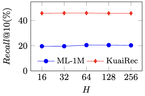
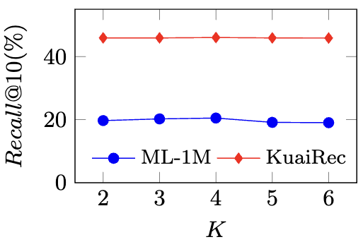
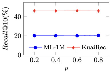
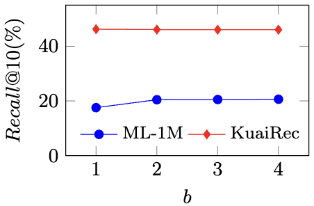
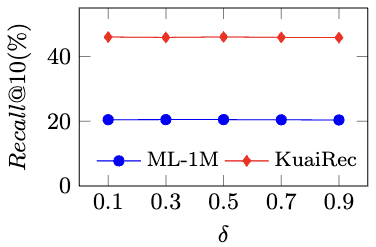
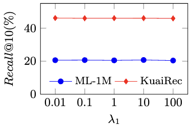
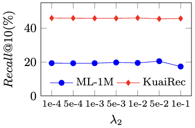
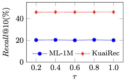
To evaluate the sensitivity of PANE-GNN to different hyperparameters, we conduct a comprehensive hyperparameter sensitivity analysis on ML-1M and KuaiRec. We systematically vary the values of key hyperparameters and measure their impact on the model performance in terms of $Recall@10$. The results are shown in Figure 4 and the following findings were observed:

• GNNs layer number $K$: As shown in Figure 4 (b), we observed that the $Recall@10$ metric initially increases with an increasing number of GNNs layers on the ML-1M dataset. However, beyond a certain point, the $Recall@10$ value starts to decrease. This observation aligns with the phenomenon of over-smoothing, where an excessive number of GNNs layers can cause the aggregation of node embeddings to become too similar, resulting in the loss of discriminative information. Additionally, as the number of GNNs layers increases, the computational efficiency of the model may be negatively impacted. Considering both the risk of over-smoothing and computational efficiency, we recommend setting $K$ as 3 or 4 to ensure good recommendation outcomes while maintaining computational efficiency.

• Feedback-aware coefficient $b$: From the analysis of Figure 4 (d), we observed that $b=1$ resulted in inferior performance compared to other values of $b$ on ML-1M. It indicates that discriminating between positive and negative feedback during the optimization process is crucial for achieving better results on ML-1M. The suboptimal performance of $b=1$ suggests that the model might not adequately capture the discriminative signals between positive and negative feedback when they are given equal weight. On the KuaiRec dataset, the stability of PANE-GNN’s performance and its insensitivity to different values of $b$ suggest that the dataset’s inherent characteristics might diminish the significance of distinguishing between positive and negative feedback. Based on these observations, we recommend setting $b$ as 2 or 3.

• Regularization coefficient $\lambda_{2}$: As shown in Figure 4 (g), $\lambda_{2}=0.1$ performs worst compared with others on ML-1M and KuaiRec. Although the L2 regularization term in Eq. (16) can prevent overfitting, high $\lambda_{2}$ excessively penalizes the model’s parameters, resulting in underfitting. Hence, we suggest selecting $\lambda_{2}$ from the range of [0.01, 0.05] for PANE-GNN.

• Others: We found that PANE-GNN demonstrates robustness to various other hyperparameters, including the edge removing ratio $p$ and contrastive learning coefficient $\lambda_{1}$.

4.5.4. Case study (RQ4)

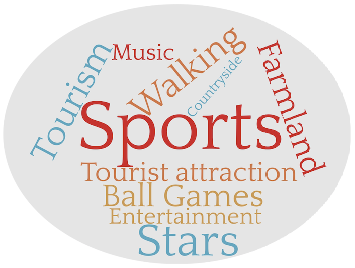
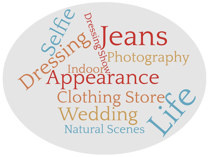
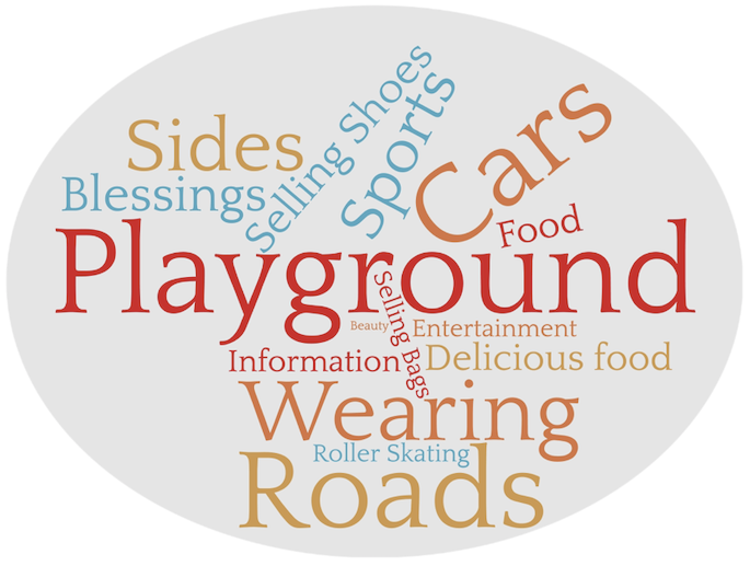
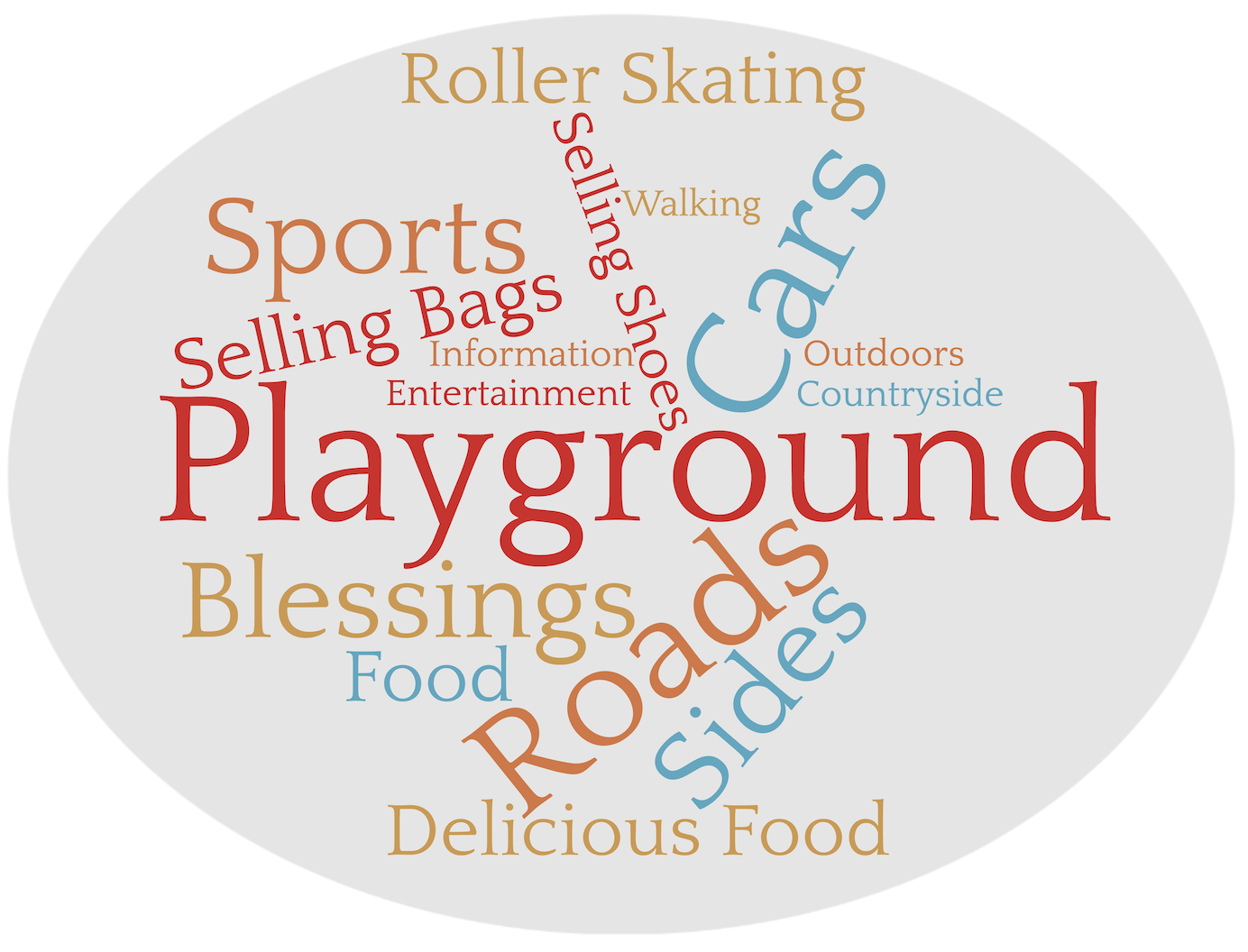
In this subsection, we evaluate the recommendation quality of PANE-GNN by analyzing the tag information of videos in KuaiRec. In Figure 5 (a), we observe that the user has a preference for outdoor sports-related videos based on the tags of liked videos in the training set. Conversely, Figure 5 (b) displays the tags of disliked videos, indicating disinterest in videos related to dressing or clothing. Figure 5 (c) and Figure 5 (d) depict the tags of the recommended videos generated by PANE-GNN before and after the filtering process, respectively. Our observations reveal the following insights: In Figure 5 (c), the recommended videos generated by PANE-GNN generally align with the user’s interests depicted in Figure 5 (a), except for a few specific words such as “Wearing” and “Beauty”. With the disinterest-score filter (Figure 5 (d)), PANE-GNN successfully filters out less relevant recommendations, while suggesting more relevant videos with tags like “Walking”, “Outdoors”, and “Countryside”. These findings emphasize two key points: 1) PANE-GNN effectively captures both user interests and disinterests from the training data, and 2) the implementation of the disinterest-score filter proves to be an effective approach for generating more relevant recommendation outcomes.

5. Conclusion and Future Work

In this work, we address the problem of leveraging negative feedback to improve recommender systems. Existing approaches in the literature focused on GNN-based recommendation models that only consider message passing on the positive graph. To overcome this limitation and capture high-order structural information from both positive and negative graphs, we propose a novel GNN-based recommendation model called PANE-GNN. By aggregating and updating messages on these two graphs, we enable the model to effectively incorporate positive and negative feedback. Additionally, we employ contrastive learning on the negative graph to reduce noise and filter out items with high disinterest scores, ensuring the relevance of the recommended results. Experimental evaluations conducted on four real-world datasets demonstrate that PANE-GNN consistently outperforms state-of-the-art GNN-based recommendation methods. We also conduct an in-depth analysis of PANE-GNN to validate its effectiveness across different components and its robustness to hyperparameters. In the future, we plan to investigate the exposure bias issue in GNN-based recommendation models.

References

- (1)
- Alshehri and Zhang (2022) Manal A. Alshehri and Xiangliang Zhang. 2022. Generative Adversarial Zero-Shot Learning for Cold-Start News Recommendation. In Proceedings of the 31st ACM International Conference on Information & Knowledge Management, Atlanta, GA, USA, October 17-21, 2022. ACM, 26–36.
- Chen et al. (2021) Chong Chen, Weizhi Ma, Min Zhang, Zhaowei Wang, Xiuqiang He, Chenyang Wang, Yiqun Liu, and Shaoping Ma. 2021. Graph heterogeneous multi-relational recommendation. In Proceedings of the AAAI Conference on Artificial Intelligence, Vol. 35. 3958–3966.
- Chen et al. (2020) Lei Chen, Le Wu, Richang Hong, Kun Zhang, and Meng Wang. 2020. Revisiting graph based collaborative filtering: A linear residual graph convolutional network approach. In Proceedings of the AAAI conference on artificial intelligence, Vol. 34. 27–34.
- Darban and Valipour (2022) Zahra Zamanzadeh Darban and Mohammad Hadi Valipour. 2022. GHRS: Graph-based hybrid recommendation system with application to movie recommendation. Expert Systems with Applications 200 (2022), 116850.
- Derr et al. (2018) Tyler Derr, Yao Ma, and Jiliang Tang. 2018. Signed graph convolutional networks. In 2018 IEEE International Conference on Data Mining (ICDM). IEEE, 929–934.
- Gao et al. (2022a) Chongming Gao, Shijun Li, Wenqiang Lei, Jiawei Chen, Biao Li, Peng Jiang, Xiangnan He, Jiaxin Mao, and Tat-Seng Chua. 2022a. KuaiRec: A Fully-observed Dataset and Insights for Evaluating Recommender Systems. In Proceedings of the 31st ACM International Conference on Information & Knowledge Management. 540–550.
- Gao et al. (2022b) Chen Gao, Xiang Wang, Xiangnan He, and Yong Li. 2022b. Graph neural networks for recommender system. In Proceedings of the Fifteenth ACM International Conference on Web Search and Data Mining. 1623–1625.
- Glorot and Bengio (2010) Xavier Glorot and Yoshua Bengio. 2010. Understanding the difficulty of training deep feedforward neural networks. In Proceedings of the thirteenth international conference on artificial intelligence and statistics. JMLR Workshop and Conference Proceedings, 249–256.
- Gong et al. (2022) Xudong Gong, Qinlin Feng, Yuan Zhang, Jiangling Qin, Weijie Ding, Biao Li, Peng Jiang, and Kun Gai. 2022. Real-time Short Video Recommendation on Mobile Devices. In Proceedings of the 31st ACM International Conference on Information & Knowledge Management. 3103–3112.
- Gong et al. (2020) Yu Gong, Ziwen Jiang, Yufei Feng, Binbin Hu, Kaiqi Zhao, Qingwen Liu, and Wenwu Ou. 2020. EdgeRec: recommender system on edge in Mobile Taobao. In Proceedings of the 29th ACM International Conference on Information & Knowledge Management. 2477–2484.
- He and McAuley (2016) Ruining He and Julian McAuley. 2016. VBPR: visual bayesian personalized ranking from implicit feedback. In Proceedings of the AAAI conference on artificial intelligence, Vol. 30.
- He et al. (2020) Xiangnan He, Kuan Deng, Xiang Wang, Yan Li, Yongdong Zhang, and Meng Wang. 2020. Lightgcn: Simplifying and powering graph convolution network for recommendation. In Proceedings of the 43rd International ACM SIGIR conference on research and development in Information Retrieval. 639–648.
- He et al. (2017) Xiangnan He, Lizi Liao, Hanwang Zhang, Liqiang Nie, Xia Hu, and Tat-Seng Chua. 2017. Neural collaborative filtering. In Proceedings of the 26th international conference on world wide web. 173–182.
- Huang et al. (2021a) Junjie Huang, Huawei Shen, Qi Cao, Shuchang Tao, and Xueqi Cheng. 2021a. Signed Bipartite Graph Neural Networks. In Proceedings of the 30th ACM International Conference on Information & Knowledge Management. 740–749.
- Huang et al. (2021b) Junjie Huang, Huawei Shen, Liang Hou, and Xueqi Cheng. 2021b. SDGNN: Learning Node Representation for Signed Directed Networks. In Thirty-Fifth AAAI Conference on Artificial Intelligence, AAAI 2021, Thirty-Third Conference on Innovative Applications of Artificial Intelligence, IAAI 2021, The Eleventh Symposium on Educational Advances in Artificial Intelligence, EAAI 2021, Virtual Event, February 2-9, 2021. AAAI Press, 196–203.
- Hwang and Chae (2022a) Sunghyun Hwang and Dong-Kyu Chae. 2022a. An Uncertainty-Aware Imputation Framework for Alleviating the Sparsity Problem in Collaborative Filtering. In Proceedings of the 31st ACM International Conference on Information & Knowledge Management. 802–811.
- Hwang and Chae (2022b) Sunghyun Hwang and Dong-Kyu Chae. 2022b. An Uncertainty-Aware Imputation Framework for Alleviating the Sparsity Problem in Collaborative Filtering. In Proceedings of the 31st ACM International Conference on Information & Knowledge Management. 802–811.
- Kim et al. (2022) Taeri Kim, Yeon-Chang Lee, Kijung Shin, and Sang-Wook Kim. 2022. MARIO: Modality-Aware Attention and Modality-Preserving Decoders for Multimedia Recommendation. In Proceedings of the 31st ACM International Conference on Information & Knowledge Management. 993–1002.
- Kingma and Ba (2015) Diederik P. Kingma and Jimmy Ba. 2015. Adam: A Method for Stochastic Optimization. In 3rd International Conference on Learning Representations, ICLR 2015, San Diego, CA, USA, May 7-9, 2015, Conference Track Proceedings.
- Kipf and Welling (2017) Thomas N. Kipf and Max Welling. 2017. Semi-Supervised Classification with Graph Convolutional Networks. In 5th International Conference on Learning Representations, ICLR 2017, Toulon, France, April 24-26, 2017, Conference Track Proceedings. OpenReview.net.
- Lee et al. (2020) Yeon-Chang Lee, Nayoun Seo, Kyungsik Han, and Sang-Wook Kim. 2020. Asine: Adversarial signed network embedding. In Proceedings of the 43rd international acm sigir conference on research and development in information retrieval. 609–618.
- Li et al. (2020) Yu Li, Yuan Tian, Jiawei Zhang, and Yi Chang. 2020. Learning signed network embedding via graph attention. In Proceedings of the AAAI Conference on Artificial Intelligence, Vol. 34. 4772–4779.
- Liu et al. (2022) Han Liu, Yinwei Wei, Jianhua Yin, and Liqiang Nie. 2022. Hs-gcn: Hamming spatial graph convolutional networks for recommendation. IEEE Transactions on Knowledge and Data Engineering (2022).
- Ning et al. (2022) Wentao Ning, Reynold Cheng, Jiajun Shen, Nur Al Hasan Haldar, Ben Kao, Xiao Yan, Nan Huo, Wai Kit Lam, Tian Li, and Bo Tang. 2022. Automatic Meta-Path Discovery for Effective Graph-Based Recommendation. In Proceedings of the 31st ACM International Conference on Information & Knowledge Management. 1563–1572.
- Oh et al. (2022) Sejoon Oh, Berk Ustun, Julian McAuley, and Srijan Kumar. 2022. Rank List Sensitivity of Recommender Systems to Interaction Perturbations. In Proceedings of the 31st ACM International Conference on Information & Knowledge Management. 1584–1594.
- Pang et al. (2022) Yitong Pang, Lingfei Wu, Qi Shen, Yiming Zhang, Zhihua Wei, Fangli Xu, Ethan Chang, Bo Long, and Jian Pei. 2022. Heterogeneous global graph neural networks for personalized session-based recommendation. In Proceedings of the fifteenth ACM international conference on web search and data mining. 775–783.
- Qin et al. (2022) Yuqi Qin, Pengfei Wang, Biyu Ma, and Zhe Zhang. 2022. A Multi-Interest Evolution Story: Applying Psychology in Query-based Recommendation for Inferring Customer Intention. In Proceedings of the 31st ACM International Conference on Information & Knowledge Management. 1655–1665.
- Rendle et al. (2009) Steffen Rendle, Christoph Freudenthaler, Zeno Gantner, and Lars Schmidt-Thieme. 2009. BPR: Bayesian Personalized Ranking from Implicit Feedback. In UAI 2009, Proceedings of the Twenty-Fifth Conference on Uncertainty in Artificial Intelligence, Montreal, QC, Canada, June 18-21, 2009. AUAI Press, 452–461.
- Rendle et al. (2012) Steffen Rendle, Christoph Freudenthaler, Zeno Gantner, and Lars Schmidt-Thieme. 2012. BPR: Bayesian Personalized Ranking from Implicit Feedback. CoRR abs/1205.2618 (2012).
- Seo et al. (2022) Changwon Seo, Kyeong-Joong Jeong, Sungsu Lim, and Won-Yong Shin. 2022. SiReN: Sign-Aware Recommendation Using Graph Neural Networks. IEEE Transactions on Neural Networks and Learning Systems (2022).
- van den Oord et al. (2018) Aäron van den Oord, Yazhe Li, and Oriol Vinyals. 2018. Representation Learning with Contrastive Predictive Coding. CoRR abs/1807.03748 (2018).
- Wang et al. (2019) Xiang Wang, Xiangnan He, Meng Wang, Fuli Feng, and Tat-Seng Chua. 2019. Neural graph collaborative filtering. In Proceedings of the 42nd international ACM SIGIR conference on Research and development in Information Retrieval. 165–174.
- Wu et al. (2023) Chuhan Wu, Fangzhao Wu, Yongfeng Huang, and Xing Xie. 2023. Personalized news recommendation: Methods and Challenges. ACM Transactions on Information Systems 41, 1 (2023), 1–50.
- Wu et al. (2022a) Le Wu, Xiangnan He, Xiang Wang, Kun Zhang, and Meng Wang. 2022a. A survey on accuracy-oriented neural recommendation: From collaborative filtering to information-rich recommendation. IEEE Transactions on Knowledge and Data Engineering (2022).
- Wu et al. (2022b) Shiwen Wu, Fei Sun, Wentao Zhang, Xu Xie, and Bin Cui. 2022b. Graph neural networks in recommender systems: a survey. Comput. Surveys 55, 5 (2022), 1–37.
- Xu et al. (2021) Pinghua Xu, Wenbin Hu, Jia Wu, Weiwei Liu, Yang Yang, and Philip Yu. 2021. Signed Network Representation by Preserving Multi-order Signed Proximity. IEEE Transactions on Knowledge and Data Engineering (2021).
- Xu et al. (2022) Pinghua Xu, Yibing Zhan, Liu Liu, Baosheng Yu, Bo Du, Jia Wu, and Wenbin Hu. 2022. Dual-branch density ratio estimation for signed network embedding. In Proceedings of the ACM Web Conference 2022. 1651–1662.
- Yoo et al. (2022) Hyunsik Yoo, Yeon-Chang Lee, Kijung Shin, and Sang-Wook Kim. 2022. Directed Network Embedding with Virtual Negative Edges. In WSDM ’22: The Fifteenth ACM International Conference on Web Search and Data Mining, Virtual Event / Tempe, AZ, USA, February 21 - 25, 2022. ACM, 1291–1299.
- Yu et al. (2022a) Sizhe Yu, Ziyi Liu, Shixiang Wan, Jia Zheng, Zang Li, and Fan Zhou. 2022a. MDP2 Forest: A Constrained Continuous Multi-dimensional Policy Optimization Approach for Short-video Recommendation. In Proceedings of the 28th ACM SIGKDD Conference on Knowledge Discovery and Data Mining. 2388–2398.
- Yu et al. (2022b) Wenhui Yu, Zixin Zhang, and Zheng Qin. 2022b. Low-Pass Graph Convolutional Network for Recommendation. In Proceedings of the AAAI Conference on Artificial Intelligence, Vol. 36. 8954–8961.
- Zhang et al. (2022) Xuanyu Zhang, Qing Yang, and Dongliang Xu. 2022. DeepVT: Deep View-Temporal Interaction Network for News Recommendation. In Proceedings of the 31st ACM International Conference on Information & Knowledge Management. 2640–2650.
- Zheng et al. (2023) Ruiqi Zheng, Liang Qu, Bin Cui, Yuhui Shi, and Hongzhi Yin. 2023. AutoML for Deep Recommender Systems: A Survey. ACM Transactions on Information Systems (2023).