Master Integrals for Electroweak corrections to $gg\rightarrow\gamma\gamma$ - Light quark contributions

Abstract

We present a calculation of the master integrals (MI’s) required for the calculation of the Electroweak corrections to $gg\rightarrow\gamma\gamma$ production in which the process contains a light quark loop. The integrals can be broken down into five categories based on the flow of the heavy vector bosons throughout the loop. Three of the families are planar, and two are non-planar. We determine a canonical basis for each family which allows an efficient solution of the resulting differential equations via iterated integrals. We calculate the families in relevant physical kinematics and obtain an efficient numerical evaluation based on an implementation of Chen-iterated integrals.

1 Introduction

The production of prompt photon pairs has long been a staple process at hadron colliders with many observations ranging back over the last four decades Bonvin:1988yu ; Alitti:1992hn ; Abe:1992cy ; Abazov:2010ah ; Aaltonen:2012jd ; Chatrchyan:2011qt ; Aad:2012tba ; Aad:2013zba ; Aaltonen:2011vk ; Chatrchyan:2013mwa ; Chatrchyan:2014fsa ; Marini:2016zjr ; CMS:2018qao ; ALICE:2019rtd ; ATLAS:2019buk ; ATLAS:2019iaa ; CMS:2019jlq ; ATLAS:2021mbt ; ATLAS:2023yrt . A centerpiece of this work and culmination of many years of effort was the discovery of the Higgs boson in this channel in 2012 Aad:2012tfa ; Chatrchyan:2012ufa . Going forward into the era of the High Luminosity LHC (HL-LHC) the process will continue to be studied in ever greater experimental precision, mandating a continued theoretical effort to provide increasingly accurate predictions for this channel.

At the lowest order in perturbation theory the production of photon pairs proceeds through a $q\overline{q}$ annihilation channel. For many years the theoretical state of the art corresponded to Next-to-Leading Order (NLO) QCD predictions, implemented into the Monte Carlo code Diphox Binoth:1999qq . However over the last decade significant theoretical progress has been made, including Next-to-Next-to Leading Order (NNLO) QCD predictions Campbell:2016yrh ; Catani:2011qz and $q_{T}$ resummed predictions at order N³LL matched to NNLO Neumann:2021zkb . Further, the theoretical predictions in association with one or more jets is well under control DelDuca:2003uz ; Gehrmann:2013bga ; Badger:2013ava ; Chawdhry:2021hkp . These results, in combination with recent computation of the three-loop amplitudes for $q\overline{q}\rightarrow\gamma\gamma$ Caola:2020dfu suggests that it is not unreasonable to assume the availability of N³LO predictions over the course of the HL-LHC.

At $\mathcal{O}(\alpha_{s}^{2})$ (NNLO in QCD) the gluon-initiated $gg\rightarrow\gamma\gamma$ partonic configuration becomes accessible for the first time. For LHC kinematics there is a large flux of gluons, which somewhat compensates the suppression from the increased powers of the coupling. Thus for a long time Glover:1988fe the $gg$ initiated production of vector boson pairs has received special attention in the theoretical literature. The NLO QCD corrections to this process (which corresponds to two-loop diagrams) for massless quarks were presented around twenty years ago in refs. Bern:2001df ; Bern:2002jx and more recently massive top loops have also been included at this order Chen:2019fla ; Maltoni:2018zvp . The three-loop $gg\rightarrow\gamma\gamma$ calculation Bargiela:2021wuy and two-loop $gg\rightarrow g\gamma\gamma$ amplitudes (for light quarks) has further extended the known theoretical structure of this process in QCD.

One of the reasons the $gg$ initiated process is so fascinating is its role in the continued study of the Higgs boson. The $gg\rightarrow\gamma\gamma$ amplitude interferes with the amplitude for the production of a Higgs boson through a top loop and subsequent decay to photons. This interference can lead to changes in the measured properties of the Higgs Martin:2012xc ; Dixon:2003yb ; Dixon:2013haa when compared to a signal only theoretical predictions. These initial studies have generated significant interest, leading to calculations over a wider range of production modes deFlorian:2013psa ; Coradeschi:2015tna ; Campbell:2017rke . In particular, it has been noted that the interference, and hence width extraction, is sensitive to higher order corrections in QCD Cieri:2017kpq ; Bargiela:2022dla . This motivates the study of the electroweak corrections to the interference pattern, of which the starting point is provided in this paper by the calculation of two-loop integrals required.

Over the last decade signifiant progress has been made in the computation of multi-loop Feynman integrals due to the advances related to solution via differential equations. Using differential equations to simplify and solve Feynman integrals is a well-established technique Kotikov:1990kg ; Remiddi:1997ny ; Gehrmann:1999as ; Gehrmann:2000xj ; Argeri:2007up , however, the field experienced a major advance when, in ref. Henn:2013pwa , a refined basis approach was proposed. By modifying the basis from a traditional one, derived for instance via reduction by integration by parts identities, ref. Henn:2013pwa proposed a new canonical basis which obeyed a simpler differential equation which factorized the regulating parameter from the kinematics. If such a basis can be found, solutions to the differential equation can be more readily extracted. Since its introduction, the canonical differential equation technique has led to the calculation of many two-loop process for $2\rightarrow 2$ and even $2\rightarrow 3$ kinematics; for an incomplete list see e.g. Gehrmann:2001ck ; Bonciani:2016ypc ; DiVita:2017xlr ; Heller:2019gkq ; Hasan:2020vwn ; Bonetti:2020hqh ; Behring:2020cqi ; Canko:2020ylt ; Duhr:2021fhk ; Abreu:2021smk ; Bonciani:2021zzf ; Kardos:2022tpo ; Abreu:2022vei ; Badger:2022hno ; Armadillo:2022bgm ; Bonetti:2022lrk ; Buccioni:2022kgy .

One of the negative features of calculations beyond one-loop is the lack of common basis. This means that typically each new calculation often requires a dedicated calculation of the relevant MIs for the process, further since different authors use different normalizing factors and conventions, it is often inconvenient or impractical to combine results from different MI calculations. Our aim is to calculate the electroweak corrections to $gg\rightarrow\gamma\gamma$, in this first paper we present the MIs for the simplest set of Feynman diagrams, namely those which proceed through a loop of quarks which can be taken to be massless. Although more complicated MI calculations have been performed in the literature, we were unable to find specific MIs for several of our topologies (relating to diagrams involving three massive $W$ bosons radiating photons). We therefore believe it is worthwhile to discuss these integrals in one place with a consistent framework. We postpone the discussion of the third generation quark loops, which contain many new MIs, to a future publication.

This paper proceeds as follows, in Section 2 we present a discussion of the canonical basis, and the solution of the differential equation via Chen-iterated integrals. Section 3 then presents the calculation of the planar topologies and section 4 presents the calculation of the non-planar topologies, finally we draw our conclusions in section 5. Electronic files containing solutions obtained in this paper are included as ancillary files with this paper.

2 Overview

The primary focus of this paper is the calculation of the Master Integrals (MI’s) required for the evaluation of the electroweak (EW) corrections to the $gg\rightarrow\gamma\gamma$ process which proceeds through the following kinematic reaction

$$0\rightarrow g(k_{1})+g(k_{2})+\gamma(k_{3})+\gamma(k_{4}),$$ (1)

where we consider all external momenta to be outgoing, and light-like ($k_{i}^{2}=0$). It is convenient to parameterize the scattering in terms of the following Mandelstam invariants

$$s\!=\!(k_{1}\!+\!k_{2})^{2}=2k_{1}\cdot k_{2},$$

$$\;t\!=\!(k_{2}\!+\!k_{3})^{2}=2k_{2}\cdot k_{3},$$

$$\;u\!=\!(k_{1}\!+\!k_{3})^{2}=2k_{1}\cdot k_{3}.$$ (2)

Momentum conservation further constrains the sum of the Mandelstam invariants $s+t+u=0$, and for physical scatterings $s>0$ and $u,t<0$. We employ the ’t Hooft-Veltman scheme in which loop momenta are evaluated in $d=4-2\epsilon$ dimensions and polarization vectors $(\epsilon_{i})$ and momenta attributed to the final state bosons are taken in four dimensions. We also note that when computing loop topologies later in this paper we introduce the momenta set $p_{1},p_{2}$ and $p_{3}$, where the assigned signs of $p_{i}\cdot p_{j}$ can vary based on which of the $k_{i}$ we assign to each $p_{j}$.

We define the $\ell$-loop color stripped amplitude as follows

$${A}_{\ell}^{a_{1}a_{2}}=16\pi^{2}\delta^{a_{1}a_{2}}\alpha^{0}_{s}\alpha^{0}\,\mathcal{A}_{\ell}(s,t),\;$$ (3)

where $\alpha^{0}_{s}$ represents the bare strong and $\alpha^{0}$ denotes the bare electromagnetic coupling, $\delta^{a_{1}a_{2}}$ defines the leading order QCD color factor. In our calculation we will decompose the amplitude into a series of tensor structures following the procedure outlined in refs. Peraro:2019cjj ; Peraro:2020sfm . In total there are eight relevant tensor structures

$$\mathcal{A}(s,t)=\sum_{i=1}^{8}{F}_{i}\>T_{i}.$$ (4)

Here the tensors $T_{i}$ are defined as:

$$T_{1}=\epsilon_{1}\!\cdot\!k_{3}\;\epsilon_{2}\!\cdot\!k_{1}\;\epsilon_{3}\!\cdot\!k_{1}\;\epsilon_{4}\!\cdot\!k_{2}\;,$$

$$T_{2}=\epsilon_{1}\!\cdot\!k_{3}\;\epsilon_{2}\!\cdot\!k_{1}\;\epsilon_{3}\!\cdot\!\epsilon_{4},\quad T_{3}=\epsilon_{1}\!\cdot\!k_{3}\;\epsilon_{3}\!\cdot\!k_{1}\;\epsilon_{2}\!\cdot\!\epsilon_{4},$$

$$T_{4}=\epsilon_{1}\!\cdot\!k_{3}\;\epsilon_{4}\!\cdot\!k_{2}\;\epsilon_{2}\!\cdot\!\epsilon_{3},\quad T_{5}=\epsilon_{2}\!\cdot\!k_{1}\;\epsilon_{3}\!\cdot\!k_{1}\;\epsilon_{1}\!\cdot\!\epsilon_{4},$$

$$T_{6}=\epsilon_{2}\!\cdot\!k_{1}\;\epsilon_{4}\!\cdot\!k_{2}\;\epsilon_{1}\!\cdot\!\epsilon_{3},\quad T_{7}=\epsilon_{3}\!\cdot\!k_{1}\;\epsilon_{4}\!\cdot\!k_{2}\;\epsilon_{1}\!\cdot\!\epsilon_{2},$$

$$T_{8}=\epsilon_{1}\!\cdot\!\epsilon_{2}\;\epsilon_{3}\!\cdot\!\epsilon_{4}+\epsilon_{1}\!\cdot\!\epsilon_{4}\;\epsilon_{2}\!\cdot\!\epsilon_{3}+\epsilon_{1}\!\cdot\!\epsilon_{3}\;\epsilon_{2}\!\cdot\!\epsilon_{4}\;.$$ (5)

Each tensor has a corresponding form-factor ${F}_{i}$. In defining the tensor decomposition we make the cyclic gauge choice $\epsilon_{i}\!\cdot\!k_{i+1}=0$, with $k_{5}=k_{1}$ and impose the transversality condition $\epsilon_{i}\!\cdot\!k_{i}=0$. We use projector operators in order to isolate individual form factors entering into the expansion in eq. 4. Each projector is defined through an orthogonality condition with the corresponding tensor such that $\sum_{pol}P_{i}T_{j}=\delta_{ij}$. Since the resulting projectors are the same as those appearing in the literature  Peraro:2019cjj ; Peraro:2020sfm ; Bargiela:2021wuy we do not list them explicitly here for the sake of brevity.

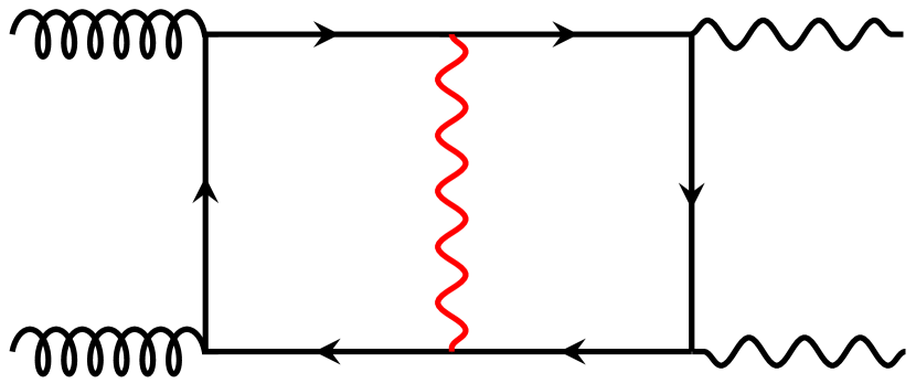
(a) Topology P${}_{\text{I}}$

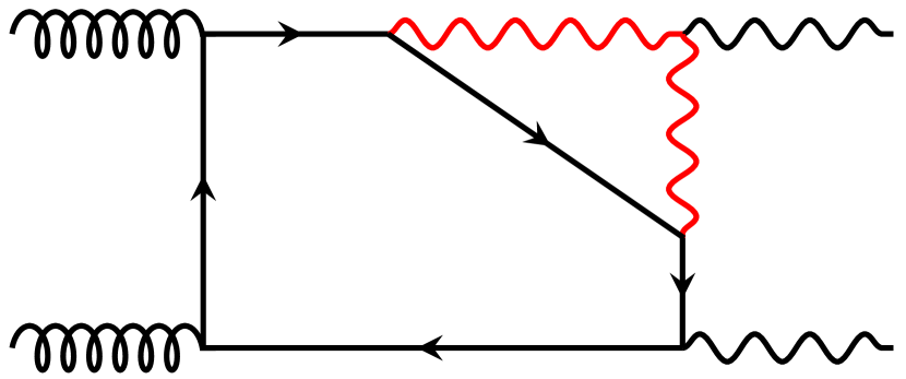
(b) Topology P${}_{\text{II}}$

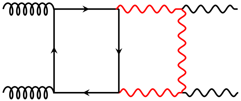
(c) Topology P${}_{\text{III}}$

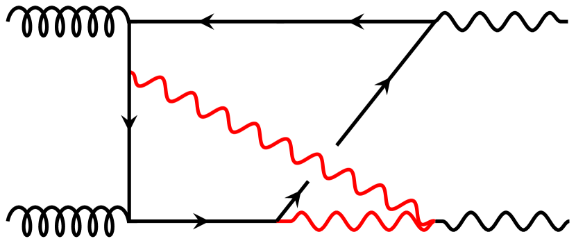
(d) Topology N${}_{\text{I}}$

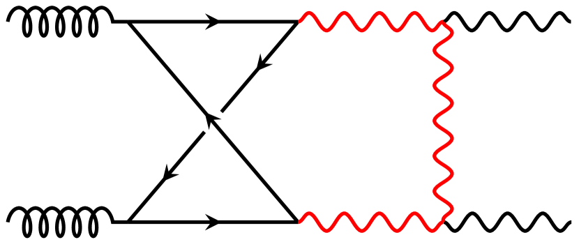
(e) Topology N${}_{\text{II}}$

Figure 1: Feynman diagrams associated with the relevant topologies. Propagators marked in red are massive.

The lowest order $gg\rightarrow\gamma\gamma$ amplitude occurs at $\mathcal{O}(\alpha_{s}\alpha)$ and proceeds through a closed loop of quarks. Here we are interested in EW corrections to the lowest order amplitude and are therefore calculating two-loop topologies. As a step towards the full $\mathcal{O}(\alpha)$ corrections we present in this work the MIs associated with quark loops arising from the first two generations ($q=u,d,c,s$) for which the quark mass can be set to zero. We postpone analysis of the third generation to a future publication. We work in the t’Hooft-Feynman gauge with $\xi=1$. The resulting diagrams can be classified in terms of five-master topologies, three planar and two non-planar for which representative Feynman diagrams are shown in Fig.1. We note that four of the topologies $\text{P}_{\text{I-III}}$ and $\text{N}_{\text{I}}$ are also relevant for the mixed QCD-EW corrections to $q\overline{q}\to\gamma\gamma$, whereas $\text{N}_{\text{II}}$ can only occur with a closed loop of fermions. We note that, in addition to the topologies listed above which all contain at least one massive boson, there are contributions from a photon exchange. However, these contributions are well understood from the studies of $gg\rightarrow gg$ (see e.g. Henn:2013pwa for a canonical basis for these integrals) and we do not consider them explicitly in this paper (although we have checked our results obtained for these diagrams against the literature, finding perfect agreement).

After computing the two-loop diagrams and applying the projectors described above the resulting the form-factors consist of thousands of unique scalar integrals. However, through the application of well-known reduction techniques the amplitude can be written in terms of a much smaller set of Master Integrals (MI’s). The choice of MIs is not unique, however, and a judicious choice is a set which satisfy differential equations of the following form Henn:2013pwa

$$\frac{\partial}{\partial x_{i}}\vec{\mathcal{G}}(\{x_{i}\})=\epsilon\mathcal{A}(\{x_{i}\})\,\vec{\mathcal{G}}(\{x_{i}\}),$$ (6)

here $\vec{\mathcal{G}}(\{{x}_{i}\})$ denotes the vector constructed from the MI’s which depend on the external scales $x_{i}$ (typically chosen to be dimensionless ratios). $\mathcal{A}(\{x_{i}\})$ is a matrix which depends on these external scales, but crucially not on the dimensional regulating parameter $\epsilon$. In this case the kinematics have factorized from the $\epsilon$-series expansion and the integrals are said to be in canonical form. If such a basis can be found, the solution to the above differential equation can readily be obtained, and the MIs can be written as the following Chen iterated integral Chen:1977oja ; Caron-Huot:2014lda

$$\vec{\mathcal{G}}(\{x_{i}\})=\left(\mathbbm{1}+\epsilon\int_{\gamma}d\mathcal{A}+\epsilon^{2}\int_{\gamma}d\mathcal{A}\,d\mathcal{A}+\dots\right)\vec{\mathcal{G}}(\{x^{0}_{i}\}).$$ (7)

Here $\gamma$ is defined as a smooth map $\gamma:[0,1]\to D\forall p\in D$ such that $\gamma(0)=\{x^{0}_{i}\}$ and $\gamma(1)=\{x_{i}\}$ and $\vec{\mathcal{G}}(\{x^{0}_{i}\})$ denotes a boundary vector which must be determined by independent means. If such a boundary vector is known, then the solution is obtained at a given weight by successive integrations over the integration kernel $d\mathcal{A}$. The value of the integral does not depend on the chosen path $\gamma$, provided no singular points (or branch cuts) are crossed. By writing the vector of MIs as a series expansion in $\epsilon$ through $\epsilon^{4}$,

$$\vec{\mathcal{G}}(\{x_{i}\})=\sum_{j=0}^{4}\epsilon^{j}\vec{\mathcal{G}}^{(j)}(\{x_{i}\}),$$ (8)

and comparing to eq. 7, we can quickly define each coefficient:

$$\vec{\mathcal{G}}^{(1)}(\{x_{i}\})=\int_{\gamma}d\mathcal{A}\,\vec{\mathcal{G}}^{(0)}(\{x^{0}_{i}\})+\vec{\mathcal{G}}^{(1)}(\{x^{0}_{i}\}),$$ (9)

$$\vec{\mathcal{G}}^{(2)}(\{x_{i}\})=\int_{\gamma}d\mathcal{A}\,d\mathcal{A}\,\vec{\mathcal{G}}^{(0)}(\{x^{0}_{i}\})+\int_{\gamma}d\mathcal{A}\,\vec{\mathcal{G}}^{(1)}(\{x^{0}_{i}\})+\vec{\mathcal{G}}^{(2)}(\{x^{0}_{i}\}),$$ (10)

$$\vec{\mathcal{G}}^{(3)}(\{x_{i}\})=\int_{\gamma}d\mathcal{A}\,d\mathcal{A}\,d\mathcal{A}\,\vec{\mathcal{G}}^{(0)}(\{x^{0}_{i}\})+\int_{\gamma}d\mathcal{A}\,d\mathcal{A}\,\vec{\mathcal{G}}^{(1)}(\{x^{0}_{i}\})+\int_{\gamma}d\mathcal{A}\,\vec{\mathcal{G}}^{(2)}(\{x^{0}_{i}\})$$

$$\hskip 45.0pt+\vec{\mathcal{G}}^{(3)}(\{x^{0}_{i}\}),$$ (11)

$$\vec{\mathcal{G}}^{(4)}(\{x_{i}\})=\int_{\gamma}d\mathcal{A}\,d\mathcal{A}\,d\mathcal{A}\,d\mathcal{A}\,\vec{\mathcal{G}}^{(0)}(\{x^{0}_{i}\})+\int_{\gamma}d\mathcal{A}\,d\mathcal{A}\,d\mathcal{A}\,\vec{\mathcal{G}}^{(1)}(\{x^{0}_{i}\})+\int_{\gamma}d\mathcal{A}\,d\mathcal{A}\,\vec{\mathcal{G}}^{(2)}(\{x^{0}_{i}\})$$

$$\hskip 45.0pt+\int_{\gamma}d\mathcal{A}\,\vec{\mathcal{G}}^{(3)}(\{x^{0}_{i}\})+\vec{\mathcal{G}}^{(4)}(\{x^{0}_{i}\}).$$ (12)

A pleasing feature of the canonical basis is that at a given order in $\epsilon$ every term has equal transcendental weight (equal to the power of $\epsilon$ expanded to). It is convenient to write the integration kernel in a $dlog$ form as follows

$$d\mathcal{A}=\sum_{k}\mathcal{M}_{k}\;d\log{\eta_{k}},$$ (13)

where $\eta_{k}$ defines a letter, $\mathcal{M}_{k}$ is the coefficient matrix relative to said letter and the set of all letters $\{\eta_{k}\}$ defines the alphabet of the problem. Following the notation in ref. Bonciani:2016ypc we see that, when expanded to a given weight each term which enters the solution is of the form

$$\int_{\gamma}d\log{\eta_{k_{j}}}\dots d\log{\eta_{k_{1}}}=\int_{0\leq t_{1}\leq\dots\leq t_{j}\leq 1}g^{\gamma}_{k_{j}}(t_{j})\dots g^{\gamma}_{k_{1}}(t_{1})dt_{1}\dots dt_{j},$$ (14)

where

$$g_{k}^{\gamma}(t)=\frac{d}{dt}\log{\eta_{k}(\gamma(t))},$$ (15)

defines the integration of the letter along the chosen path. Following the notation of ref. Bonciani:2016ypc once more, we can more compactly define

$$C^{[\gamma]}_{k_{j}\dots k_{i}}\equiv\int_{\gamma}d\log{\eta_{k_{j}}}\dots d\log{\eta_{k_{i}}}.$$ (16)

Our solution is then made up of many terms with different orderings of the letters $k_{j}\dots k_{i}$. If all of the letters are rational then the term may be written in terms of the well-known Goncharov polylogarithms:

$$G(a;x_{0}) =\int_{0}^{x_{0}}\frac{dt}{t-a},$$ (17)

$$G(a_{n},\dots,a_{1};x_{0}) =\int_{0}^{x_{0}}G(a_{n-1},\dots,a_{1};x_{0})\frac{dt}{t-a_{n}},$$ (18)

$$G(\vec{0}_{n};x_{0}) =\frac{1}{n!}\log{(x_{0})}^{n}.$$ (19)

However, we will frequently encounter non-rational letters which must be directly integrated through eq. 14. Nominally one would expect to perform $k$-integrations to obtain a weight-$k$ contribution, however Chen-iterated integrals have several pleasing properties which can systematically reduce the complexity of the problem. We refer interested readers to the more complete overviews which can be found, for instance, in ref. Bonciani:2016ypc . Here we note only the most important identities required in our calculation. Firstly we note that at weight one, path independence renders the integration trivial, one must simply evaluate the integral at its end-points.

Then at weight two one can use this to perform the inner most integration and then perform the following integration by parts identity writing

$$C^{[\gamma]}_{ab}=\int_{0}^{1}g_{b}(t)(\log{\eta_{a}({\bf{x}}(t)})-\log{\eta_{a}({{\bf{x}}_{0})})dt},$$ (20)

such that all weight two contributions can be written as single parameter integrals. Once all weight two functions are obtained one can systematically reduce the number of integrations, by using the following generalized integration by parts identity

$$C^{[\gamma]}_{k_{j}\dots k_{i}}=\log{\eta_{k_{j}}({\bf{x}}})\;C^{[\gamma]}_{k_{j-1}\dots k_{i}}-\int\log{\eta_{k_{j}}({\bf{x}}(t))}\;g_{k_{j-1}}(t)\;C^{[\gamma_{t}]}_{k_{j-2}\dots k_{i}}dt,$$ (21)

where $[\gamma_{t}]$ is a modified path which integrates over the domain $[0,t]$ (and the complete path is restored as $t\rightarrow 1$). Up to weight four order we therefore are able to write weight three contributions as one parameter integrals, and weight four contributions as integrals over two parameters. Finally, situations frequently occur when the inner most letter vanishes at the boundary of integration, which introduces potential singular contributions. In order to extract and remove theses contributions we employ a shuffle algebra to systematically extract singular logarithms (and cancel them with the corresponding terms arising at the boundary)

$$C^{[\gamma]}_{{\boldsymbol{k}}}C^{[\gamma]}_{{\boldsymbol{j}}}=\sum_{\rm{shuffles}\;\;\sigma}C^{[\gamma]}_{\sigma(k_{k}),\dots\sigma(k_{1}),\sigma(j_{j}),\dots,\sigma(j_{1})},$$ (22)

where ${\boldsymbol{k}}$ and ${\boldsymbol{j}}$ are the vectors of letters with length $k$ and $j$ and the sum runs over all permutations which preserve the relative order of ${\boldsymbol{k}}$ and ${\boldsymbol{j}}$.

Our general setup is as follows: starting from the relevant Feynman diagrams for each topology we project out the form factors obtaining scalar integrals. These are then reduced using Kira 2.0 Klappert:2020nbg ; Maierhofer:2017gsa to a minimal set of MIs. We then promote the obtained basis to canonical form using the Magnus-Dyson approach outlined in ref. Argeri:2014qva . We then use the physical properties of the Feynman integrals to determine boundaries at special kinematic points. Our final answers are then obtained via path integration away from these boundary vectors. In all instances we are able to check our results numerically using the package AMFlow Liu:2022chg (we have additionally checked with pySecDec Borowka:2015mxa where possible too). During our calculations we make frequent use of the software PolyLogTools Duhr:2019tlz and HandyG Naterop:2019xaf . The next sections describe these calculations in detail.

3 Planar Topologies

3.1 Planar topology P${}_{\text{I}}$

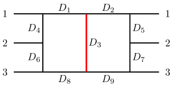
Figure 2: The auxiliary topology diagram for P${}_{\text{I}}$ as defined in Eq. 3.1. Propagators marked in red are massive.

The first planar topology we encounter involves the exchange of a single massive boson. The associated propagator structure has the following form

$$I^{\text{P}_{\text{I}}}_{a_{1}\dots a_{9}}=\left(\frac{M_{W}^{2\epsilon}}{\Gamma({\epsilon})}\right)^{2}\int\frac{d^{d}\ell_{1}}{(2\pi)^{d}}\frac{d^{d}\ell_{2}}{(2\pi)^{d}}\frac{1}{D_{1}^{a_{1}}D_{2}^{a_{2}}D_{3}^{a_{3}}D_{4}^{a_{4}}D_{5}^{a_{5}}D_{6}^{a_{6}}D_{7}^{a_{7}}D_{8}^{a_{8}}D_{9}^{a_{9}}},$$ (23)

with

$$D_{1}=\ell_{1}^{2}, D_{2}=\ell_{2}^{2}, D_{3}=(\ell_{1}+\ell_{2})^{2}-M_{W}^{2},$$

$$D_{4}=(\ell_{1}-p_{1})^{2}, D_{5}=(\ell_{2}+p_{1})^{2}, D_{6}=(\ell_{1}-p_{1}-p_{2})^{2},$$

$$D_{7}=(\ell_{2}+p_{1}+p_{2})^{2}, D_{8}=(\ell_{1}-p_{1}-p_{2}-p_{3})^{2}, D_{9}=(\ell_{2}+p_{1}+p_{2}+p_{3})^{2}.$$ (24)

These propagators form an auxiliary topology which is presented in Fig. 2. We note that, since the external momentum $\{k_{i}\}$ can be permuted into any ordering, we need to evaluate this topology in three distinct regions defined by the signs of $p_{i}\cdot p_{j}$. All the integrals that appear in the physical amplitude can be expressed, via integration by parts identities (IBPs), in terms of a minimal basis of Master Integrals (MIs). We used Kira Klappert:2020nbg to obtain such set of identities and we found that for the sum over all Feynman diagrams with a single massive boson with a fixed order of the final state momentum we need a total of 25 MIs. Therefore, in order to obtain a basis in canonical form we start with the following 25 integrals:

$$\mathcal{J}_{1} ={\bf{D}}^{-}(I^{\text{P}_{\text{I}}}_{111000000}), \mathcal{J}_{2} ={\bf{D}}^{-}(I^{\text{P}_{\text{I}}}_{101001000}), \mathcal{J}_{3} ={\bf{D}}^{-}(I^{\text{P}_{\text{I}}}_{011001000}),$$

$$\mathcal{J}_{4} ={\bf{D}}^{-}(I^{\text{P}_{\text{I}}}_{(-1)11001000}), \mathcal{J}_{5} ={\bf{D}}^{-}(I^{\text{P}_{\text{I}}}_{001100010}), \mathcal{J}_{6} ={\bf{D}}^{-}(I^{\text{P}_{\text{I}}}_{001010010}),$$

$$\mathcal{J}_{7} ={\bf{D}}^{-}(I^{\text{P}_{\text{I}}}_{(-1)01010010}), \mathcal{J}_{8} =I^{\text{P}_{\text{I}}}_{102011000}, \mathcal{J}_{9} =I^{\text{P}_{\text{I}}}_{101021000},$$

$$\mathcal{J}_{10} =I^{\text{P}_{\text{I}}}_{012100010}, \mathcal{J}_{11} =I^{\text{P}_{\text{I}}}_{021100010}, \mathcal{J}_{12} ={\bf{D}}^{-}(I^{\text{P}_{\text{I}}}_{000110011}),$$

$$\mathcal{J}_{13} =I^{\text{P}_{\text{I}}}_{111011000}, \mathcal{J}_{14} =I^{\text{P}_{\text{I}}}_{111010010}, \mathcal{J}_{15} =I^{\text{P}_{\text{I}}}_{101101010},$$

$$\mathcal{J}_{16} =I^{\text{P}_{\text{I}}}_{011101010}, \mathcal{J}_{17} =I^{\text{P}_{\text{I}}}_{012101010}, \mathcal{J}_{18} =I^{\text{P}_{\text{I}}}_{101011010},$$

$$\mathcal{J}_{19} =I^{\text{P}_{\text{I}}}_{102011010}, \mathcal{J}_{20} =I^{\text{P}_{\text{I}}}_{011011010}, \mathcal{J}_{21} =I^{\text{P}_{\text{I}}}_{012011010},$$

$$\mathcal{J}_{22} =I^{\text{P}_{\text{I}}}_{001110011}, \mathcal{J}_{23} =I^{\text{P}_{\text{I}}}_{011111011}, \mathcal{J}_{24} =I^{\text{P}_{\text{I}}}_{(-1)11111011},$$

$$\mathcal{J}_{25} =I^{\text{P}_{\text{I}}}_{(-1)11111(-1)11},$$ (25)

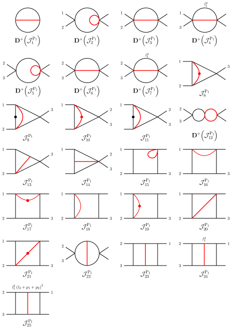
Figure 3: Master integrals for the P${}_{\text{I}}$ topology. Dotted propagators have higher power of the respective denominator, while red propagators are massive.

which are presented in Fig. 3. It is convenient to write some of these integrals using the dimension shifting operator

$${\bf{D}}^{-}(I^{\text{P}_{\text{I}}}_{a_{1}\dots a_{9}}) = \bigg{(}(a_{1}\mathbf{1}^{+}+a_{4}\mathbf{4}^{+}+a_{6}\mathbf{6}^{+}+a_{8}\mathbf{8}^{+})(a_{2}\mathbf{2}^{+}+a_{5}\mathbf{5}^{+}+a_{7}\mathbf{7}^{+}+a_{9}\mathbf{9}^{+})$$

$$+a_{3}\mathbf{3}^{+}(\sum_{j\neq 3}\,a_{j}{\mathbf{j}^{+}})\bigg{)}I^{\text{P}_{\text{I}}}_{a_{1}\dots a_{9}}.$$

Where $\mathbf{j}^{+}$ increases the power of the $j^{\rm{th}}$ propagator by one. In order to write our basis in canonical form, we introduce the following finite and dimensionless integrals

$$\mathcal{F}_{X}=\epsilon^{2}\;(M_{W})^{\alpha}\mathcal{J}_{X},$$ (27)

where $\alpha$ is defined for $\mathcal{J}_{X}=f(I^{\text{P}_{\text{I}}}_{a_{1}\dots a_{9}})$ as $(\sum{a_{i}})-4$, and we utilize the techniques of the Magus-Dyson approach outlined in ref. Argeri:2014qva to obtain the following canonical basis:

$$\mathcal{G}_{1}^{\text{P}_{\text{I}}}=\mathcal{F}_{1}, \mathcal{G}_{2}^{\text{P}_{\text{I}}}=x\mathcal{F}_{2}, \mathcal{G}_{3}^{\text{P}_{\text{I}}}=(1+x)\mathcal{F}_{3},$$

$$\mathcal{G}_{4}^{\text{P}_{\text{I}}}=\mathcal{F}_{4}-\mathcal{F}_{3}, \mathcal{G}_{5}^{\text{P}_{\text{I}}}=y\mathcal{F}_{5}, \mathcal{G}_{6}^{\text{P}_{\text{I}}}=(1+y)\mathcal{F}_{6},$$

$$\mathcal{G}_{7}^{\text{P}_{\text{I}}}=\mathcal{F}_{7}, \mathcal{G}_{8}^{\text{P}_{\text{I}}}=\epsilon x\mathcal{F}_{8}, \mathcal{G}_{9}^{\text{P}_{\text{I}}}=\epsilon x\mathcal{F}_{9},$$

$$\mathcal{G}_{10}^{\text{P}_{\text{I}}}=\epsilon y\mathcal{F}_{10}, \mathcal{G}_{11}^{\text{P}_{\text{I}}}=\epsilon y\mathcal{F}_{11}, \mathcal{G}_{12}^{\text{P}_{\text{I}}}=y^{2}\mathcal{F}_{12},$$

$$\mathcal{G}_{13}^{\text{P}_{\text{I}}}=\epsilon^{2}x\mathcal{F}_{13}, \mathcal{G}_{14}^{\text{P}_{\text{I}}}=\epsilon^{2}y\mathcal{F}_{14}, \mathcal{G}_{15}^{\text{P}_{\text{I}}}=\epsilon(\epsilon-1)xy\mathcal{F}_{15},$$

$$\mathcal{G}_{16}^{\text{P}_{\text{I}}}=\epsilon y((2\epsilon-1)\mathcal{F}_{16}+\mathcal{F}_{17}), \mathcal{G}_{17}^{\text{P}_{\text{I}}}=\epsilon xy\mathcal{F}_{17}, \mathcal{G}_{18}^{\text{P}_{\text{I}}}=\epsilon((2\epsilon-1)x\mathcal{F}_{18}+\mathcal{F}_{19}),$$

$$\mathcal{G}_{19}^{\text{P}_{\text{I}}}=\epsilon xy\mathcal{F}_{19}, \mathcal{G}_{20}^{\text{P}_{\text{I}}}=\epsilon^{2}(x+y)\mathcal{F}_{20}, \mathcal{G}_{21}^{\text{P}_{\text{I}}}=-\epsilon(x+y+xy)\mathcal{F}_{21},$$

$$\mathcal{G}_{22}^{\text{P}_{\text{I}}}=\epsilon(1-2\epsilon)y\mathcal{F}_{22}, \mathcal{G}_{23}^{\text{P}_{\text{I}}}=\epsilon^{2}(1+x)y^{2}\mathcal{F}_{23}, \mathcal{G}_{24}^{\text{P}_{\text{I}}}=\epsilon^{2}y^{2}(\mathcal{F}_{24}-\mathcal{F}_{23}),$$

$$\mathcal{G}_{25}^{\text{P}_{\text{I}}}=\mathrlap{x\left(\frac{1}{4}y\mathcal{F}_{12}+2\epsilon^{2}\mathcal{F}_{20}+y\epsilon^{2}\mathcal{F}_{23}\right)+\epsilon^{2}y(\mathcal{F}_{25}-\mathcal{F}_{22}).}$$ (28)

Here the differential equation is expressed in terms of the following dimensionless ratios,

$$x=-\frac{2p_{1}\cdot p_{2}}{M_{W}^{2}}{\qquad\text{and}\qquad}y=-\frac{2p_{2}\cdot p_{3}}{M_{W}^{2}}.$$ (29)

This basis is indeed in canonical form, and satisfies the following differential equations

$$\frac{\partial\mathcal{G}^{\text{P}_{\text{I}}}_{j}}{\partial x}=\epsilon(A_{x}\mathcal{G}^{\text{P}_{\text{I}}})_{j}\qquad\text{and}\qquad\frac{\partial\mathcal{G}^{\text{P}_{\text{I}}}_{j}}{\partial y}=\epsilon(A_{y}\mathcal{G}^{\text{P}_{\text{I}}})_{j}.$$ (30)

For this topology the MIs depend only on rational functions of $x$ and $y$. As a result, the solutions of the differential equation can be expressed in terms of Goncharov polylogarithms (GPLs) and efficiently evaluated using HandyG Naterop:2019xaf at every point in the phase space. In particular, the kinematic regions of interest in terms of the variables in Eq.29 are given by

$${\rm{Region\;\;A}}: (p_{1}\cdot p_{2}>0,\;p_{1}\cdot p_{3}<0,\;p_{2}\cdot p_{3}<0)\quad\to x<0,\;y>0,\;\lvert x\lvert>\lvert y\lvert,$$ (31)

$${\rm{Region\;\;B}}: (p_{1}\cdot p_{2}<0,\;p_{1}\cdot p_{3}>0,\;p_{2}\cdot p_{3}<0)\quad\to x>0,\;y>0,$$ (32)

$${\rm{Region\;\;C}}: (p_{1}\cdot p_{2}<0,\;p_{1}\cdot p_{3}<0,\;p_{2}\cdot p_{3}>0)\quad\to x>0,\;y<0,\;\lvert y\lvert>\lvert x\lvert.$$ (33)

The boundary conditions can be determined for these integrals as follows:

• $\mathcal{G}_{3}^{\text{P}_{\text{I}}}$ and $\mathcal{G}_{4}^{\text{P}_{\text{I}}}$ are fixed since they are finite as $x\rightarrow 0$, and in this limit $\mathcal{G}_{3}^{\text{P}_{\text{I}}}=\mathcal{G}_{1}^{\text{P}_{\text{I}}}$.

• Similarly $\mathcal{G}_{6}^{\text{P}_{\text{I}}}$ and $\mathcal{G}_{7}^{\text{P}_{\text{I}}}$ are finite as $y\rightarrow 0$, and in this limit $\mathcal{G}_{6}^{\text{P}_{\text{I}}}=\mathcal{G}_{1}^{\text{P}_{\text{I}}}$.

• $\mathcal{G}_{8}^{\text{P}_{\text{I}}}$ and $\mathcal{G}_{9}^{\text{P}_{\text{I}}}$ can be determined in terms of $\mathcal{G}_{2}^{\text{P}_{\text{I}}}$ by demanding that these integrals are finite as $x\rightarrow 0$ and noting that $\mathcal{G}_{8}^{\text{P}_{\text{I}}}$ vanishes in this limit. Further $\mathcal{G}_{2}^{\text{P}_{\text{I}}}$ can then be constrained in terms of $\mathcal{G}_{1}^{\text{P}_{\text{I}}}$ by demanding that $\mathcal{G}_{9}^{\text{P}_{\text{I}}}$ is finite as $x\rightarrow 1$. In a similar fashion integrals 10 and 11 and 5 are fixed with $x\leftrightarrow y$ in terms of $\mathcal{G}_{1}^{\text{P}_{\text{I}}}$.

• $\mathcal{G}_{12}^{\text{P}_{\text{I}}}$ is the product of two trivial one-loop integrals and can be determined quickly via direct integration.

• $\mathcal{G}_{13}^{\text{P}_{\text{I}}}$ and {$\mathcal{G}_{14}^{\text{P}_{\text{I}}},\mathcal{G}_{22}^{\text{P}_{\text{I}}}\}$ are fixed since they must vanish as $x\rightarrow 0$ and $y\rightarrow 0$ respectively.

• $\mathcal{G}_{15-21}^{\text{P}_{\text{I}}}$, and $\mathcal{G}_{23-25}^{\text{P}_{\text{I}}}$ are fixed by demanding finiteness in the limit $x\rightarrow-y$.

Our integrals are then completely determined in terms of the overall normalizing integral $\mathcal{G}_{1}^{\text{P}_{\text{I}}}$ which is easily computed by direct integration, to our required order we have

$$\mathcal{G}_{1}^{\text{P}_{\text{I}}}=-1-2\zeta_{2}\epsilon^{2}+2\zeta_{3}\epsilon^{3}-9\zeta_{4}\epsilon^{4}+\mathcal{O}(\epsilon^{5}).$$ (34)

The evaluation of these integrals for a sample point for each kinematic region is presented in Appendix A.1. We have checked our results against the numerical package AMFlow Liu:2022chg , finding perfect agreement.

3.2 Planar topology P${}_{\text{II}}$

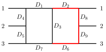
Figure 4: The auxiliary topology diagram for P${}_{\text{II}}$ as defined in Eq. 3.2. Propagators marked in red are massive.

The second planar topology we will consider arises when one external photon is radiated from a $W$-boson and the other is radiated from the quark loop. The various permutations of photons and gluons can be written as functions of the following auxiliary Feynman integral

$$I^{\text{P}_{\text{II}}}_{a_{1}\dots a_{9}}=\left(\frac{M_{W}^{2\epsilon}}{\Gamma({\epsilon})}\right)^{2}\int\frac{d^{d}\ell_{1}}{(2\pi)^{d}}\frac{d^{d}\ell_{2}}{(2\pi)^{d}}\frac{1}{D_{1}^{a_{1}}D_{2}^{a_{2}}D_{3}^{a_{3}}D_{4}^{a_{4}}D_{5}^{a_{5}}D_{6}^{a_{6}}D_{7}^{a_{7}}D_{8}^{a_{8}}D_{9}^{a_{9}}},$$ (35)

where:

$$D_{1}=\ell_{1}^{2}, D_{2}=\ell_{2}^{2}-M_{W}^{2}, D_{3}=(\ell_{1}+\ell_{2})^{2},$$

$$D_{4}=(\ell_{1}-p_{1})^{2}, D_{5}=(\ell_{1}-p_{1}-p_{2})^{2}, D_{6}=(\ell_{2}+p_{1}+p_{2}+p_{3})^{2}-M_{W}^{2}$$

$$D_{7}=(\ell_{1}-p_{1}-p_{2}-p_{3})^{2}, D_{8}=(\ell_{2}+p_{1})^{2}-M_{W}^{2}, D_{9}=(\ell_{2}+p_{1}+p_{2})^{2}-M_{W}^{2}.$$ (36)

This topology is shown in Fig. 4. For contributions to $gg\rightarrow\gamma\gamma$ considered here, $D_{8}$ and $D_{9}$ do not appear with positive power. As before, by including the various permutations of physical momenta $\{k_{1},k_{2},k_{3}\}$ we find that we must calculate this auxiliary topology in two distinct regions, depending on the sign of the associated $p_{i}\cdot p_{j}$. Following the same procedure as before, we reduce all the integrals appearing in the physical amplitude using Kira Klappert:2020nbg finding that for this topology we need a total of 24 MIs. In order to derive a canonical basis we start with the following set of integrals:

$$\mathcal{J}_{1}={\bf{D}}^{-}(I^{\text{P}_{\text{II}}}_{111000000}),\quad \mathcal{J}_{2}={\bf{D}}^{-}(I^{\text{P}_{\text{II}}}_{110010000}),\quad \mathcal{J}_{3}={\bf{D}}^{-}(I^{\text{P}_{\text{II}}}_{011010000}),$$

$$\mathcal{J}_{4}={\bf{D}}^{-}(I^{\text{P}_{\text{II}}}_{(-1)11010000}),\quad \mathcal{J}_{5}={\bf{D}}^{-}(I^{\text{P}_{\text{II}}}_{001101000}),\quad \mathcal{J}_{6}={\bf{D}}^{-}(I^{\text{P}_{\text{II}}}_{(-1)01101000}),$$

$$\mathcal{J}_{7}={\bf{D}}^{-}(I^{\text{P}_{\text{II}}}_{010100100}),\quad \mathcal{J}_{8}=I^{\text{P}_{\text{II}}}_{201011000},\quad \mathcal{J}_{9}=I^{\text{P}_{\text{II}}}_{101012000},$$

$$\mathcal{J}_{10}=I^{\text{P}_{\text{II}}}_{021100100},\quad \mathcal{J}_{11}=I^{\text{P}_{\text{II}}}_{012100100},\quad \mathcal{J}_{12}=I^{\text{P}_{\text{II}}}_{111101000},$$

$$\mathcal{J}_{13}=I^{\text{P}_{\text{II}}}_{111011000},\quad \mathcal{J}_{14}=I^{\text{P}_{\text{II}}}_{112011000},\quad \mathcal{J}_{15}=I^{\text{P}_{\text{II}}}_{101111000},$$

$$\mathcal{J}_{16}=I^{\text{P}_{\text{II}}}_{101112000},\quad \mathcal{J}_{17}=I^{\text{P}_{\text{II}}}_{011111000},\quad \mathcal{J}_{18}=I^{\text{P}_{\text{II}}}_{012111000},$$

$$\mathcal{J}_{19}=I^{\text{P}_{\text{II}}}_{110110100},\quad \mathcal{J}_{20}=I^{\text{P}_{\text{II}}}_{011110100},\quad \mathcal{J}_{21}=I^{\text{P}_{\text{II}}}_{021110100},$$

$$\mathcal{J}_{22}=I^{\text{P}_{\text{II}}}_{011101100},\quad \mathcal{J}_{23}=I^{\text{P}_{\text{II}}}_{111111000},\quad \mathcal{J}_{24}=I^{\text{P}_{\text{II}}}_{011111100},$$

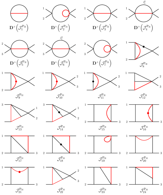
Figure 5: Master integrals for topology P${}_{\text{II}}$. Dotted propagators have higher power of the respective denominator, while red propagators are massive.

these integrals are also represented in Fig. 5. The three propagator integrals are written using the dimension shifting operator, which for this topology is defined as

$${\bf{D}}^{-}(I^{\text{P}_{\text{II}}}_{a_{1}\dots a_{9}}) = \bigg{(}(a_{1}\mathbf{1}^{+}+a_{4}\mathbf{4}^{+}+a_{5}\mathbf{5}^{+}+a_{7}\mathbf{7}^{+})(a_{2}\mathbf{2}^{+}+a_{6}\mathbf{6}^{+}a_{8}\mathbf{8}^{+}+a_{9}\mathbf{9}^{+})$$ (38)

$$+\;a_{3}\mathbf{3}^{+}\sum_{j\neq 3}\,a_{j}{\mathbf{j}^{+}}\bigg{)}I^{\text{P}_{\text{II}}}_{a_{1}\dots a_{9}}.$$

We repeat the steps outline in the previous section to rewrite our basis in canonical form by first rendering the integrals finite and dimensionless

$$\mathcal{F}_{X}=\epsilon^{2}\;(M_{W})^{\alpha}\mathcal{J}_{X},$$ (39)

and ultimately we obtain the following canonical basis:

$$\mathcal{G}_{1}^{\text{P}_{\text{II}}}=\mathcal{F}_{1}, \mathcal{G}_{2}^{\text{P}_{\text{II}}}=x\mathcal{F}_{2},\hskip 50.0pt \mathcal{G}_{3}^{\text{P}_{\text{II}}}=(1+x)\mathcal{F}_{3},$$

$$\mathcal{G}_{4}^{\text{P}_{\text{II}}}=\mathcal{F}_{4}-\mathcal{F}_{3}, \mathcal{G}_{5}^{\text{P}_{\text{II}}}=(1+y)\mathcal{F}_{5}, \mathcal{G}_{6}^{\text{P}_{\text{II}}}=\mathcal{F}_{6},$$

$$\mathcal{G}_{7}^{\text{P}_{\text{II}}}=y\mathcal{F}_{7},$$

$$\mathcal{G}_{8}^{\text{P}_{\text{II}}}=\mathrlap{\frac{2x^{2}(2\epsilon-1)\mathcal{F}_{8}+2\epsilon x(\mathcal{F}_{1}-\mathcal{F}_{9})+x\mathcal{F}_{2}}{2(x-1)},} \mathcal{G}_{9}^{\text{P}_{\text{II}}}=\epsilon x\mathcal{F}_{9},$$

$$\mathcal{G}_{10}^{\text{P}_{\text{II}}}=\epsilon y\mathcal{F}_{10}, \mathcal{G}_{11}^{\text{P}_{\text{II}}}=\epsilon y\mathcal{F}_{11}, \mathcal{G}_{12}^{\text{P}_{\text{II}}}=\epsilon^{2}y\mathcal{F}_{12},$$

$$\mathcal{G}_{13}^{\text{P}_{\text{II}}}=\epsilon^{2}x\mathcal{F}_{13}, \mathcal{G}_{14}^{\text{P}_{\text{II}}}=\epsilon x\mathcal{F}_{14}, \mathcal{G}_{15}^{\text{P}_{\text{II}}}=\epsilon x((2\epsilon-1)\mathcal{F}_{15}+\mathcal{F}_{16})$$

, $$\mathcal{G}_{16}^{\text{P}_{\text{II}}}=\epsilon xy\mathcal{F}_{16}, \mathcal{G}_{17}^{\text{P}_{\text{II}}}=\epsilon^{2}(x+y)\mathcal{F}_{17}, \mathcal{G}_{18}^{\text{P}_{\text{II}}}=\epsilon(x+y+xy)\mathcal{F}_{18},$$

$$\mathcal{G}_{19}^{\text{P}_{\text{II}}}=\epsilon(\epsilon-1)xy\mathcal{F}_{19}, \mathcal{G}_{20}^{\text{P}_{\text{II}}}=\epsilon y((2\epsilon-1)\mathcal{F}_{20}+\mathcal{F}_{21}), \mathcal{G}_{21}^{\text{P}_{\text{II}}}=\epsilon xy\mathcal{F}_{21},$$

$$\mathcal{G}_{22}^{\text{P}_{\text{II}}}=\epsilon^{2}y\mathcal{F}_{22}, \mathcal{G}_{23}^{\text{P}_{\text{II}}}=\epsilon^{2}xy\mathcal{F}_{23}, \mathcal{G}_{24}^{\text{P}_{\text{II}}}=\epsilon^{2}xy\mathcal{F}_{24},$$

where the differential equation variables are defined to the same as those in the previous topology

$$x=-\frac{2p_{1}\cdot p_{2}}{M_{W}^{2}}\quad{\rm{and}}\quad y=-\frac{2p_{2}\cdot p_{3}}{M_{W}^{2}}.$$ (41)

When considering all possible assignments of physical external momenta, we find we have to consider two kinematic regions, which we define as:

$${\rm{Region\;\;A}}: (p_{1}\cdot p_{2}>0,\;p_{1}\cdot p_{3}<0,\;p_{2}\cdot p_{3}<0)\quad\to x<0,\;y>0,\;\lvert x\lvert>\lvert y\lvert,$$ (42)

$${\rm{Region\;\;B}}: (p_{1}\cdot p_{2}<0,\;p_{1}\cdot p_{3}>0,\;p_{2}\cdot p_{3}<0)\quad\to x>0,\;y>0.$$ (43)

The basis in Eq. 3.2 is in canonical form, and satisfies the differential equations

$$\frac{\partial\mathcal{G}^{\text{P}_{\text{II}}}_{j}}{\partial x}=\epsilon(A_{x}\mathcal{G}^{\text{P}_{\text{II}}})_{j}\qquad\text{and}\qquad\frac{\partial\mathcal{G}^{\text{P}_{\text{II}}}_{j}}{\partial y}=\epsilon(A_{y}\mathcal{G}^{\text{P}_{\text{II}}})_{j},$$ (44)

where $A_{x}$ and $A_{y}$ have no dependence on $\epsilon$. Additionally, since the coefficient matrices depends only on rational functions of the variables $x$ and $y$, the solution can be written entirely in-terms of Goncharov polylogarithms and can be readily determined, once appropriate boundary conditions are known. The boundary constants can be determined as follows,

• $\mathcal{G}^{\text{P}_{\text{II}}}_{3}$ and $\mathcal{G}^{\text{P}_{\text{II}}}_{4}$ are finite as $x\rightarrow 0$, and further $\mathcal{G}^{\text{P}_{\text{II}}}_{3}=\mathcal{G}^{\text{P}_{\text{II}}}_{1}$ when $x=0$.

• The finiteness of $\mathcal{G}^{\text{P}_{\text{II}}}_{5}$ at $y=0$ fixes $\mathcal{G}^{\text{P}_{\text{II}}}_{6}$ and the relation $\mathcal{G}^{\text{P}_{\text{II}}}_{5}=\mathcal{G}^{\text{P}_{\text{II}}}_{1}$ at $y=0$ fixes $\mathcal{G}^{\text{P}_{\text{II}}}_{5}$.

• The finiteness of $\mathcal{G}^{\text{P}_{\text{II}}}_{9}$ at $x=0$ fixes $\mathcal{G}^{\text{P}_{\text{II}}}_{8}$ and the vanishing of $\mathcal{G}^{\text{P}_{\text{II}}}_{9}$ at $y=0$ fixes $\mathcal{G}^{\text{P}_{\text{II}}}_{9}$, such that $\mathcal{G}^{\text{P}_{\text{II}}}_{8}$ and $\mathcal{G}^{\text{P}_{\text{II}}}_{9}$ are determined in terms of $\mathcal{G}^{\text{P}_{\text{II}}}_{2}$. $\mathcal{G}^{\text{P}_{\text{II}}}_{2}$ can be further constrained by requiring that $\mathcal{G}^{\text{P}_{\text{II}}}_{8}$ is finite as $x\rightarrow 1$.

• The finiteness of $\mathcal{G}^{\text{P}_{\text{II}}}_{10}$ at $y=0$ and $\mathcal{G}^{\text{P}_{\text{II}}}_{11}$ at $y=1$ fixes $\mathcal{G}^{\text{P}_{\text{II}}}_{11}$ and $\mathcal{G}^{\text{P}_{\text{II}}}_{7}$. $\mathcal{G}^{\text{P}_{\text{II}}}_{10}$ can be further constrained since the integral vanishes at $y=0$.

• $\mathcal{G}^{\text{P}_{\text{II}}}_{12}$ vanishes as $y\rightarrow 0$.

• $\mathcal{G}^{\text{P}_{\text{II}}}_{13}$ and $\mathcal{G}^{\text{P}_{\text{II}}}_{14}$ vanish as $x\rightarrow 0$.

• $\mathcal{G}^{\text{P}_{\text{II}}}_{15}$ and $\mathcal{G}^{\text{P}_{\text{II}}}_{16}$, and $\mathcal{G}^{\text{P}_{\text{II}}}_{22}$ are finite as $y\rightarrow 0$.

• $\mathcal{G}^{\text{P}_{\text{II}}}_{17}$ and $\mathcal{G}^{\text{P}_{\text{II}}}_{18}$ are finite as $x\rightarrow-y$ and $x\rightarrow 0$.

• $\mathcal{G}^{\text{P}_{\text{II}}}_{19}$, $\mathcal{G}^{\text{P}_{\text{II}}}_{20}$, $\mathcal{G}^{\text{P}_{\text{II}}}_{21}$, $\mathcal{G}^{\text{P}_{\text{II}}}_{23}$ and $\mathcal{G}^{\text{P}_{\text{II}}}_{24}$ are finite as $x\rightarrow-y$.

This fixes all of our integrals in terms of the overall normalizing integral $\mathcal{G}^{\text{P}_{\text{II}}}_{1}$, which can be readily determined by direct integration:

$$\mathcal{G}^{\text{P}_{\text{II}}}_{1}=-1-2\zeta_{2}\epsilon^{2}+2\zeta_{3}\epsilon^{3}-9\zeta_{4}\epsilon^{4}+\mathcal{O}(\epsilon^{5}).$$ (45)

We note that our normzaling integral is the same as that of the $\text{P}_{\text{I}}$ topology. In obtaining the boundary conditions we made use of the PolyLogTools Duhr:2019tlz package and it’s interface to GiNaC Naterop:2019xaf to write combinations of boundary GPLs as simple functions of $\zeta_{i}$. We present results for these integrals in both regions of interest in Appendix A.2, which we obtained using HandyG Naterop:2019xaf to numerically evaluate the GPLs. We have checked our results against the numerical package AMFlow Liu:2022chg , finding perfect agreement.

3.3 Planar topology P${}_{\text{III}}$

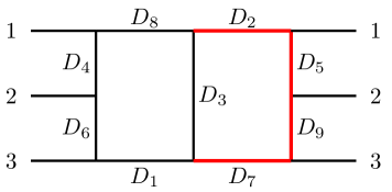
Figure 6: The auxiliary topology diagram for P${}_{\text{III}}$ as defined in Eq. 3.3. Propagators marked in red are massive.

The final, and most complicated, planar topology arises from Feynman diagrams which contain three massive vector bosons. The contributions to the form factors ${F}_{i}$ arising from the planar topology $P_{\text{III}}$ can be written in terms of the following scalar loop integral

$$I^{\text{P}_{\text{III}}}_{a_{1}\dots a_{9}}=\left(\frac{M_{W}^{2\epsilon}}{\Gamma({\epsilon})}\right)^{2}\int\frac{d^{d}\ell_{1}}{(2\pi)^{d}}\frac{d^{d}\ell_{2}}{(2\pi)^{d}}\frac{1}{D_{1}^{a_{1}}D_{2}^{a_{2}}D_{3}^{a_{3}}D_{4}^{a_{4}}D_{5}^{a_{5}}D_{6}^{a_{6}}D_{7}^{a_{7}}D_{8}^{a_{8}}D_{9}^{a_{9}}}.$$ (46)

The propagators entering the loop are defined as follows:

$$D_{1}=(\ell_{1}-p_{1}-p_{2}-p_{3})^{2}, D_{2}=\ell_{2}^{2}-M_{W}^{2}, D_{3}=(\ell_{1}+\ell_{2})^{2},$$

$$D_{4}=(\ell_{1}-p_{1})^{2}, D_{5}=(\ell_{2}+p_{1})^{2}-M_{W}^{2}, D_{6}=(\ell_{1}-p_{1}-p_{2})^{2},$$

$$D_{7}=(\ell_{2}+p_{1}+p_{2}+p_{3})^{2}-M_{W}^{2} D_{8}=\ell_{1}^{2}, D_{9}=(\ell_{2}+p_{1}+p_{2})^{2}-M_{W}^{2}.$$ (47)

These propagators form an auxiliary topology which is shown in Fig. 6. We note that this auxiliary topology is equivalent (up-to re-labeling) as that appearing in P${}_{\text{II}}$. For the physical scattering process propagators $D_{8}$ and $D_{9}$ do not appear with positive powers ($a_{8}<0$ and $a_{9}<0$). We have constructed the topology to in the same notation as topologies P${}_{\text{II}}$, which minimizes the number of unique MIs which must be computed, however this means that in order to correctly assign the physical momenta $k_{i}$ to the topology momenta $p_{i}$, mappings such as $\{p_{1},p_{2},p_{3}\}\rightarrow\{k_{3},k_{1},k_{2}\}$ must occur. For physical scattering processes we must therefore evaluate the auxiliary topology with $p_{1}\cdot p_{2}<0$ and $p_{2}\cdot p_{3}>0$. The set of scalar integrals entering the form factors from this topology can be reduced to 32 MI’s, (for which we used Kira Klappert:2020nbg ). In order to obtain a canonical basis we begin with the following set of integrals:

$$\mathcal{J}_{1}={\bf{D}}^{-}(I^{\text{P}_{\text{III}}}_{111000000}),\quad \mathcal{J}_{2}={\bf{D}}^{-}(I^{\text{P}_{\text{III}}}_{110100000}),\quad \mathcal{J}_{3}={\bf{D}}^{-}(I^{\text{P}_{\text{III}}}_{101010000}),$$

$$\mathcal{J}_{4}={\bf{D}}^{-}(I^{\text{P}_{\text{III}}}_{1(-1)1010000}),\quad \mathcal{J}_{5}={\bf{D}}^{-}(I^{\text{P}_{\text{III}}}_{011001000}),\quad \mathcal{J}_{6}={\bf{D}}^{-}(I^{\text{P}_{\text{III}}}_{(-1)11001000}),$$

$$\mathcal{J}_{7}=I^{\text{P}_{\text{III}}}_{112100000},\quad \mathcal{J}_{8}=I^{\text{P}_{\text{III}}}_{121100000},\quad \mathcal{J}_{9}=I^{\text{P}_{\text{III}}}_{102010100},$$

$$\mathcal{J}_{10}={\bf{D}}^{-}(I^{\text{P}_{\text{III}}}_{100110100}),\quad \mathcal{J}_{11}=I^{\text{P}_{\text{III}}}_{002011100},\quad \mathcal{J}_{12}=I^{\text{P}_{\text{III}}}_{001021100},$$

$$\mathcal{J}_{13}=I^{\text{P}_{\text{III}}}_{111110000},\quad \mathcal{J}_{14}=I^{\text{P}_{\text{III}}}_{112110000},\quad \mathcal{J}_{15}=I^{\text{P}_{\text{III}}}_{111101000},$$

$$\mathcal{J}_{16}=I^{\text{P}_{\text{III}}}_{121101000},\quad \mathcal{J}_{17}=I^{\text{P}_{\text{III}}}_{111011000},\quad \mathcal{J}_{18}=I^{\text{P}_{\text{III}}}_{112011000},$$

$$\mathcal{J}_{19}=I^{\text{P}_{\text{III}}}_{011111000},\quad \mathcal{J}_{20}=I^{\text{P}_{\text{III}}}_{111010100},\quad \mathcal{J}_{21}=I^{\text{P}_{\text{III}}}_{110110100},$$

$$\mathcal{J}_{22}=I^{\text{P}_{\text{III}}}_{101110100},\quad \mathcal{J}_{23}=I^{\text{P}_{\text{III}}}_{101011100},\quad \mathcal{J}_{24}=I^{\text{P}_{\text{III}}}_{011011100},$$

$$\mathcal{J}_{25}=I^{\text{P}_{\text{III}}}_{012011100},\quad \mathcal{J}_{26}=I^{\text{P}_{\text{III}}}_{111111000},\quad \mathcal{J}_{27}=I^{\text{P}_{\text{III}}}_{111110100},$$

$$\mathcal{J}_{28}=I^{\text{P}_{\text{III}}}_{111011100},\quad \mathcal{J}_{29}=I^{\text{P}_{\text{III}}}_{111111100},\quad \mathcal{J}_{30}=I^{\text{P}_{\text{III}}}_{1111111(-1)0},$$

$$\mathcal{J}_{31}=I^{\text{P}_{\text{III}}}_{11111110(-1)},\quad \mathcal{J}_{32}=I^{\text{P}_{\text{III}}}_{1111111(-1)(-1)},\quad$$ (48)

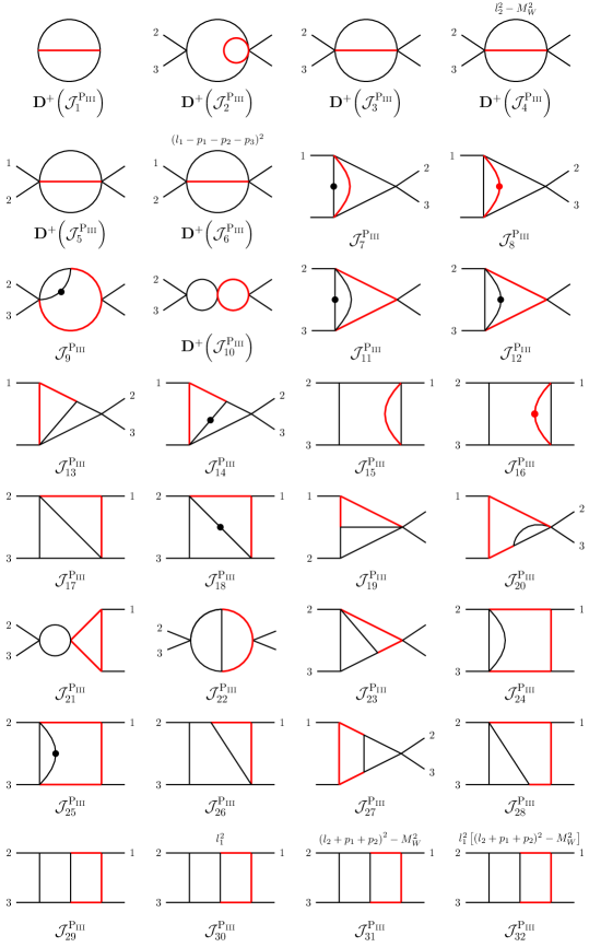
Figure 8: Master integrals for topology P${}_{\text{III}}$. Dotted propagators have higher power of the respective denominator, while red propagators are massive.

these integrals are presented in Fig. 8. Here the dimension shifting operator is defined as

$${\bf{D}}^{-}(I^{\text{P}_{\text{III}}}_{a_{1}\dots a_{9}}) = \bigg{(}(a_{1}\mathbf{1}^{+}+a_{4}\mathbf{4}^{+}+a_{6}\mathbf{6}^{+}+a_{8}\mathbf{8}^{+})(a_{2}\mathbf{2}^{+}+a_{5}\mathbf{5}^{+}a_{7}\mathbf{7}^{+}+a_{9}\mathbf{9}^{+})$$ (49)

$$+\;a_{3}\mathbf{3}^{+}\sum_{j\neq 3}\,a_{j}{\mathbf{j}^{+}}\bigg{)}I^{\text{P}_{\text{III}}}_{a_{1}\dots a_{9}}.$$

We then utilize the same strategy as the previous sections by introducing the following finite and dimensionless integrals

$$\mathcal{F}_{X}=\epsilon^{2}\,(M_{W}^{2})^{\alpha}\mathcal{J}_{X},$$ (50)

where $\alpha$ is defined for $\mathcal{J}_{X}=f(I^{\text{P}_{\text{III}}}_{a_{1}\dots a_{9}})$ as $(\sum a_{i})-4$. We can introduce the resulting basis:

$$\mathcal{G}_{1}^{\text{P}_{\text{III}}}=\mathcal{F}_{1}, \mathcal{G}_{2}^{\text{P}_{\text{III}}}=y\mathcal{F}_{2}, \mathcal{G}_{3}^{\text{P}_{\text{III}}}=(1+y)\mathcal{F}_{3},$$

$$\mathcal{G}_{4}^{\text{P}_{\text{III}}}=\mathcal{F}_{3}+\mathcal{F}_{4}, \mathcal{G}_{5}^{\text{P}_{\text{III}}}=(1+x)\mathcal{F}_{5}, \mathcal{G}_{6}^{\text{P}_{\text{III}}}=\mathcal{F}_{6},$$

$$\mathcal{G}_{7}^{\text{P}_{\text{III}}}=\epsilon y\mathcal{F}_{7}, \mathcal{G}_{8}^{\text{P}_{\text{III}}}=\epsilon y\mathcal{F}_{8},$$

$$\mathcal{G}_{9}^{\text{P}_{\text{III}}}=\mathrlap{\frac{1}{4\sqrt{r_{1}}}\left(y^{2}\mathcal{F}_{3}-2\mathcal{F}_{4}-y(\mathcal{F}_{1}-3\mathcal{F}_{3}-4\mathcal{F}_{9}+8\epsilon\mathcal{F}_{9})\right),} \mathcal{G}_{10}^{\text{P}_{\text{III}}}=y\sqrt{r_{1}}\mathcal{F}_{10},$$

$$\mathcal{G}_{11}^{\text{P}_{\text{III}}}=\epsilon y\mathcal{F}_{11}, \mathcal{G}_{12}^{\text{P}_{\text{III}}}=\frac{\sqrt{r_{1}}}{2}(\epsilon\mathcal{F}_{11}+2(2\epsilon-1)\mathcal{F}_{12}), \mathcal{G}_{13}^{\text{P}_{\text{III}}}=\epsilon^{2}y\mathcal{F}_{13},$$

$$\mathcal{G}_{14}^{\text{P}_{\text{III}}}=\epsilon y\mathcal{F}_{14}, \mathcal{G}_{15}^{\text{P}_{\text{III}}}=\epsilon y((2\epsilon-1)\mathcal{F}_{15}+\mathcal{F}_{16}), \mathcal{G}_{16}^{\text{P}_{\text{III}}}=\epsilon xy\mathcal{F}_{16},$$

$$\mathcal{G}_{17}^{\text{P}_{\text{III}}}=\epsilon^{2}(x+y)\mathcal{F}_{17}, \mathcal{G}_{18}^{\text{P}_{\text{III}}}=\epsilon(x+y+xy)\mathcal{F}_{18}, \mathcal{G}_{19}^{\text{P}_{\text{III}}}=\epsilon^{2}x\mathcal{F}_{19},$$

$$\mathcal{G}_{20}^{\text{P}_{\text{III}}}=\epsilon(2\epsilon-1)y\mathcal{F}_{20}, \mathcal{G}_{21}^{\text{P}_{\text{III}}}=\epsilon(2\epsilon-1)y\mathcal{F}_{21}, \mathcal{G}_{22}^{\text{P}_{\text{III}}}=\epsilon(2\epsilon-1)y\mathcal{F}_{22},$$

$$\mathcal{G}_{23}^{\text{P}_{\text{III}}}=\epsilon^{2}y\mathcal{F}_{23}, \mathcal{G}_{24}^{\text{P}_{\text{III}}}=\epsilon(2\epsilon-1)y\mathcal{F}_{24}, \mathcal{G}_{25}^{\text{P}_{\text{III}}}=\epsilon\sqrt{r_{2}}\mathcal{F}_{25},$$

$$\mathcal{G}_{26}^{\text{P}_{\text{III}}}=\epsilon^{2}xy\mathcal{F}_{26}, \mathcal{G}_{27}^{\text{P}_{\text{III}}}=\epsilon^{2}y\sqrt{r_{1}}\mathcal{F}_{27}, \mathcal{G}_{28}^{\text{P}_{\text{III}}}=\epsilon^{2}\sqrt{r_{3}}\mathcal{F}_{28},$$

$$\mathcal{G}_{29}^{\text{P}_{\text{III}}}=\epsilon^{2}y\sqrt{r_{2}}\mathcal{F}_{29}, \mathcal{G}_{30}^{\text{P}_{\text{III}}}=\epsilon^{2}\sqrt{r_{1}}(2x\mathcal{F}_{28}+xy\mathcal{F}_{29}+y\mathcal{F}_{30}), \mathcal{G}_{31}^{\text{P}_{\text{III}}}=\epsilon^{2}y^{2}(\mathcal{F}_{29}+\mathcal{F}_{31}),$$

$$\mathcal{G}_{32}^{\text{P}_{\text{III}}}=\mathrlap{-\frac{1}{2}\epsilon\bigg{(}2x(1-2\epsilon)\mathcal{F}_{21}+y^{2}\epsilon(-\mathcal{F}_{27}+x\mathcal{F}_{29}+\mathcal{F}_{30})}$$

$$\mathrlap{\hskip 30.0pt+2y\epsilon(2\mathcal{F}_{17}+\mathcal{F}_{22}+x\mathcal{F}_{28}+x\mathcal{F}_{29}-\mathcal{F}_{32})\bigg{)}.}$$

where we have introduced the two dimensionless ratios (which are the same as those used in the previous planar topologies)

$$x=-\frac{2p_{1}\cdot p_{2}}{M_{W}^{2}}{\qquad\text{and}\qquad}y=-\frac{2p_{2}\cdot p_{3}}{M_{W}^{2}}.$$ (52)

For physical kinematics, since both photons are radiated from the $W$ bosons, there is only one region to consider $x>0$ and $y<0$, and in the physical region $|x|\leq|y|$. In the differential equations the following roots occur

$$r_{1}=y(4+y), r_{2}=y\left(y+2xy+x^{2}(4+y)\right), r_{3}=xy\;(4y+x(4+y)).$$ (53)

In principle it is possible to rationalize two of these roots simultaneously ($r_{3}$ and $r_{1}$), however the resulting variables are quartic in two parameters, which leads to a proliferation of letters entering the Chen-integrals. In this paper we pursue an approach which rationalizes just $r_{1}$, and results in a smaller alphabet, but with more letters with non-rational components. We find this leads to a more optimal final numerical implementation in our framework. There are two sub-regions of interest, corresponding to whether or not $y$ is above the threshold at $y=-4$. We define Region A for $y\in[0,-4]$ and define

$$y=-\frac{4z_{A}^{2}}{1+z_{A}^{2}}\quad{\rm{with}}\quad 0\geq y\geq-4,$$ (54)

we take $z_{A}>0$ and therefore $x+xz_{A}^{2}<4z_{A}^{2}$ ensures $x\leq-y$. Region B is defined as $y\in(-4,-\infty)$ and here we write

$$y=-\frac{4}{1-z_{B}^{2}}\quad{\rm{with}}\quad y\leq-4,$$ (55)

with $z_{B}\in(0,1)$. In terms of these variables the differential equations take the following $dlog$-form

$$d\mathcal{A}=\sum_{k}\mathcal{M}_{k}\;d\log{\eta_{k}}$$ (56)

where the alphabet $\{\eta_{k}\}$ is made from twenty-two letters which may be inspected in the attached ancillary files. The remaining non-rational functions which enter the alphabet are

$$f^{A}_{1}=x-4z_{A}^{2}\quad{\rm{and}}\quad f^{A}_{2}=x^{2}-z_{A}^{2}-2xz_{A}^{2},$$ (57)

in region A, and

$$f^{B}_{1}=4+xz_{B}^{2}\quad{\rm{and}}\quad f^{B}_{2}=1+2x+x^{2}z_{B}^{2},$$ (58)

in region B. We have written our alphabet in a form which allows for clean extraction in the limit $x\rightarrow 0$. In terms of $(x,z_{A/B})$ variables, the following 25 MIs contain only rational letters and may be evaluated in terms of GPLs

$$\mathcal{G}_{i}^{\text{P}_{\text{III}}}\;{\rm{with}}\quad i\in\{1-23,26,27\}.$$ (59)

Many of these integrals are recycled from the previous planar topologies, the boundary conditions for the new integrals can be quickly determined via appropriate finiteness of vanishing of the integral in the limits $x\rightarrow 0$, $y\rightarrow 0$ and $x\rightarrow-y$, of which the vanishing of the integrals as $y\rightarrow 0$ is particularly useful. This procedure systematically relates MIs to one another (expanded through weight 5 to extract the pertinent limits), up to an overall normalizing integral which we again take be $\mathcal{G}^{\text{P}_{\text{III}}}_{1}$. This integral can be readily computed via direct integration and in our normalization we have

$$\mathcal{G}^{\text{P}_{\text{III}}}_{1}=-1-2\zeta_{2}\epsilon^{2}+2\zeta_{3}\epsilon^{3}-9\zeta_{4}\epsilon^{4}+\mathcal{O}(\epsilon^{5}),$$ (60)

which is the same as that used in the previous planar topologies. We evaluate GPLs using the HandyG Naterop:2019xaf package, and have also made extensive use of the PolyLogTools Duhr:2019tlz package and it’s interface to GiNaC Naterop:2019xaf to write combinations of boundary GPLs as simple functions of $\zeta_{i}$ and $\log{2}$.

The remaining 7 integrals $\{\mathcal{G}_{24}^{\text{P}_{\text{III}}},\mathcal{G}_{25}^{\text{P}_{\text{III}}},\mathcal{G}_{28-32}^{\text{P}_{\text{III}}}\}$ contain non-rational letters and cannot be evaluated in terms of pure GPLs. As discussed in section 2, a convenient means to evaluate the solution is through Chen-iterated integrals. The pre-requisite for evaluation is the knowledge of the MIs at a boundary point, such that the MIs at any other point can be determined by path integration. For our calculation the remaining task is thus to determine appropriate boundary conditions to evaluate our Chen-iterated integral expressions.

In order to solve for boundary points we note the following limit

$$\lim_{x\rightarrow 0}\left(\frac{\partial\mathcal{G}^{\text{P}_{\text{III}}}_{j}}{\partial z_{A}}\right),$$ (61)

is regular, and further is free of non-rational functions. We can therefore solve along the $x=0$ boundary entirely in terms of GPL solutions, with letters drawn from the following set

$$\{0,\pm i,\pm{1}/{\sqrt{3}},\pm{i}/{\sqrt{5}}\},$$ (62)

in region A. The unknown boundary constants attributed to the 7 integrals with non-rational functions in the bulk space can be quickly determined through the vanishing of the integrals as $y\rightarrow 0$ or ($z_{A}\rightarrow 0$). The equivalent boundary GPLs in Region B can be obtained from these results via analytic continuation (using $z_{A}=i/z_{B}$) when $y<-4$. We have written our alphabet to allow smooth extraction of the $x\rightarrow 0$ limit, however in doing so we introduce the spurious letter $\eta_{1}=1-2x$, which introduces a (spurious) singularity in region A. In order to avoid paths which cross the resulting branch cut, we also solve the following differential equations

$$\lim_{x\rightarrow-y}\left(\frac{\partial\mathcal{G}^{\text{P}_{\text{III}}}_{j}}{\partial z_{A}}\right),$$ (63)

which again, is entirely made up of GPL solutions (with the same letters as eq. 62), and known boundary constants. For region B, the boundary solutions at $x=0$ are sufficient.

With our boundary constants in hand we are therefore able to evaluate the remaining 7 integrals via path integration starting at the boundary points described aboves. We present results for all integrals evaluated at specific phase space points in Appendix A.3. In order to demonstrate the flexibility of our code we present the evaluation of the most complicated 7 point integrals along the arbitrary line $y=-2.6x-1$ where we show results from $x=1$ to $x=3$ in Fig.7. We made this choice to compactly demonstrate the lack of issues around $x=1/2$ and to evaluate the integrals above and below threshold. Also shown in the figure is a comparison to the result obtained using the numerical package AMFlow Liu:2022chg with a point taken in each region. We have checked all of our integrals with AMFlow and we find perfect agreement within to the reported uncertainty from the numerical codes.

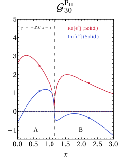
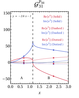
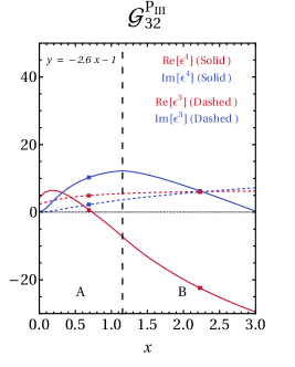
Figure 7: Coefficients of the $\epsilon^{i}$ terms (where $i=2,3,4$) in the expansion of the three 7 point integrals $\mathcal{G}^{\text{P}_{\text{III}}}_{30}$, $\mathcal{G}^{\text{P}_{\text{III}}}_{31}$, and $\mathcal{G}^{\text{P}_{\text{III}}}_{32}$. Here $x\in[0,3]$ and $y$ is varied along the line $y=-2.6x-1$ between Region A and Region B, as defined in Eq.54 and Eq.55 respectively. Red and blue squares represent the real and imaginary part, respectively, of independent evaluation using AMFlow.

4 Non-planar topologies

4.1 Non-planar topology N${}_{\text{I}}$

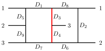
Figure 9: Auxiliary Topology diagram for N${}_{\text{I}}$ as defined in Eq. 4.1. Propagators marked in red are massive.

The first non-planar topology which we encounter occurs when a single photon is radiated from the massive line and has the following propagator structure

$$I^{\text{N}_{\text{I}}}_{a_{1}\dots a_{9}}=\left(\frac{M_{W}^{2\epsilon}}{\Gamma(\epsilon)}\right)^{2}\int\frac{d^{d}\ell_{1}}{(2\pi)^{d}}\frac{d^{d}\ell_{2}}{(2\pi)^{d}}\frac{1}{D_{1}^{a_{1}}D_{2}^{a_{2}}D_{3}^{a_{3}}D_{4}^{a_{4}}D_{5}^{a_{5}}D_{6}^{a_{6}}D_{7}^{a_{7}}D_{8}^{a_{8}}D_{9}^{a_{9}}},$$ (64)

with:

$$D_{1}=\ell_{1}^{2}, D_{2}=(\ell_{2}+p_{1})^{2}, D_{3}=(\ell_{1}+\ell_{2})^{2}-M_{W}^{2},$$

$$D_{4}=(\ell_{1}+\ell_{2}-p_{3})^{2}-M_{W}^{2}, D_{5}=(\ell_{1}-p_{1})^{2}, D_{6}=(\ell_{2}+p_{1}+p_{2})^{2},$$

$$D_{7}=(\ell_{1}-p_{1}-p_{2}-p_{3})^{2}, D_{8}=\ell_{2}^{2}, D_{9}=(\ell_{1}-p_{1}-p_{2})^{2}.$$ (65)

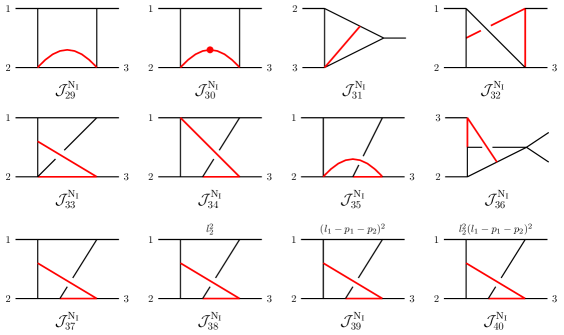
Figure 10: Master integrals for topology N${}_{\text{I}}$. Dotted propagators have higher power of the respective denominator, while red propagators are massive

These propagators form an auxiliary topology which is presented in Fig. 9. For physical scattering permutations of the external photons and gluons require us to evaluate the integral in all possible kinematic regions, e.g. with $p_{1}\cdot p_{2}$ and $p_{2}\cdot p_{3}$ having signs $(+-)$, $(-+)$ and $(--)$. In order to evaulate the Feynman diagrams occurring in this topology, 40 MI’s are required. As a starting point we introduce the following 40 integral combinations (which are presented in Fig. 10):

$$\mathcal{J}_{1}={\bf{D}}^{-}(I^{\text{N}_{\text{I}}}_{111000000}),\quad \mathcal{J}_{2}={\bf{D}}^{-}(I^{\text{N}_{\text{I}}}_{110100000}),\quad \mathcal{J}_{3}={\bf{D}}^{-}(I^{\text{N}_{\text{I}}}_{11(-1)100000}),$$

$$\mathcal{J}_{4}={\bf{D}}^{-}(I^{\text{N}_{\text{I}}}_{101001000}),\quad \mathcal{J}_{5}={\bf{D}}^{-}(I^{\text{N}_{\text{I}}}_{1(-1)1001000}),\quad \mathcal{J}_{6}={\bf{D}}^{-}(I^{\text{N}_{\text{I}}}_{000111000}),$$

$$\mathcal{J}_{7}={\bf{D}}^{-}(I^{\text{N}_{\text{I}}}_{(-1)00111000}),\quad \mathcal{J}_{8}={\bf{D}}^{-}(I^{\text{N}_{\text{I}}}_{001010100}),\quad \mathcal{J}_{9}=I^{\text{N}_{\text{I}}}_{010210100},$$

$$\mathcal{J}_{10}=I^{\text{N}_{\text{I}}}_{010220100},\quad \mathcal{J}_{11}=I^{\text{N}_{\text{I}}}_{111110000},\quad \mathcal{J}_{12}=I^{\text{N}_{\text{I}}}_{111101000},$$

$$\mathcal{J}_{13}=I^{\text{N}_{\text{I}}}_{211101000},\quad \mathcal{J}_{14}=I^{\text{N}_{\text{I}}}_{111011000},\quad \mathcal{J}_{15}=I^{\text{N}_{\text{I}}}_{110111000},$$

$$\mathcal{J}_{16}=I^{\text{N}_{\text{I}}}_{110211000},\quad \mathcal{J}_{17}=I^{\text{N}_{\text{I}}}_{101111000},\quad \mathcal{J}_{18}=I^{\text{N}_{\text{I}}}_{201111000},$$

$$\mathcal{J}_{19}=I^{\text{N}_{\text{I}}}_{011111000},\quad \mathcal{J}_{20}=I^{\text{N}_{\text{I}}}_{111100100},\quad \mathcal{J}_{21}=I^{\text{N}_{\text{I}}}_{211100100},$$

$$\mathcal{J}_{22}=I^{\text{N}_{\text{I}}}_{110110100},\quad \mathcal{J}_{23}=I^{\text{N}_{\text{I}}}_{110210100},\quad \mathcal{J}_{24}=I^{\text{N}_{\text{I}}}_{011110100},$$

$$\mathcal{J}_{25}=I^{\text{N}_{\text{I}}}_{111001100},\quad \mathcal{J}_{26}=I^{\text{N}_{\text{I}}}_{112001100},\quad \mathcal{J}_{27}=I^{\text{N}_{\text{I}}}_{110101100},$$

$$\mathcal{J}_{28}=I^{\text{N}_{\text{I}}}_{101101100},\quad \mathcal{J}_{29}=I^{\text{N}_{\text{I}}}_{101011100},\quad \mathcal{J}_{30}=I^{\text{N}_{\text{I}}}_{102011100},$$

$$\mathcal{J}_{31}=I^{\text{N}_{\text{I}}}_{011011100},\quad \mathcal{J}_{32}=I^{\text{N}_{\text{I}}}_{111111000},\quad \mathcal{J}_{33}=I^{\text{N}_{\text{I}}}_{111110100},$$

$$\mathcal{J}_{34}=I^{\text{N}_{\text{I}}}_{111101100},\quad \mathcal{J}_{35}=I^{\text{N}_{\text{I}}}_{101111100},\quad \mathcal{J}_{36}=I^{\text{N}_{\text{I}}}_{011111100},$$

$$\mathcal{J}_{37}=I^{\text{N}_{\text{I}}}_{111111100},\quad \mathcal{J}_{38}=I^{\text{N}_{\text{I}}}_{1111111(-1)0},\quad \mathcal{J}_{39}=I^{\text{N}_{\text{I}}}_{11111110(-1)},$$

$$\mathcal{J}_{40}=I^{\text{N}_{\text{I}}}_{1111111(-1)(-1)}.\quad$$ (66)

Here the dimension shifting operator is defined as

$${\bf{D}}^{-}(I^{\text{N}_{\text{I}}}_{a_{1}\dots a_{9}}) = \bigg{(}(a_{1}\mathbf{1}^{+}+a_{5}\mathbf{5}^{+}+a_{7}\mathbf{7}^{+}+a_{9}\mathbf{9}^{+})(a_{2}\mathbf{2}^{+}+a_{6}\mathbf{6}^{+}+a_{8}\mathbf{8}^{+})$$ (67)

$$+(a_{3}\mathbf{3}^{+}+a_{4}\mathbf{4}^{+})(\sum_{j\neq 3,4}\,a_{j}{\mathbf{j}^{+}})\bigg{)}I^{\text{N}_{\text{I}}}_{a_{1}\dots a_{9}}.$$

As before we begin by rescaling the integrals to become dimensionless

$$\mathcal{F}_{X}=\epsilon^{2}\;M_{W}^{2\alpha}\mathcal{J}_{X},$$ (68)

where again, $\alpha$ is defined for $\mathcal{J}_{X}=f(I^{\text{N}_{\text{I}}}_{a_{1}\dots a_{9}})$ as $(\sum{a_{i}})-4$. Introducing the following dimensionless ratios

$$x=\frac{2p_{1}\cdot p_{2}}{M_{W}^{2}},\quad{\rm{and}}\quad y=\frac{2p_{1}\cdot p_{3}}{M_{W}^{2}}.$$ (69)

We can write a canonical basis as follows:

$$\mathcal{G}^{\text{N}_{\text{I}}}_{1}=\mathcal{F}_{1}, \mathcal{G}^{\text{N}_{\text{I}}}_{2}=(1-y)\mathcal{F}_{2}, \mathcal{G}^{\text{N}_{\text{I}}}_{3}=\mathcal{F}_{2}+\mathcal{F}_{3},$$

$$\mathcal{G}^{\text{N}_{\text{I}}}_{4}=(1-x)\mathcal{F}_{4}, \mathcal{G}^{\text{N}_{\text{I}}}_{5}=\mathcal{F}_{5}, \mathcal{G}^{\text{N}_{\text{I}}}_{6}=(1+x+y)\mathcal{F}_{6},$$

$$\mathcal{G}^{\text{N}_{\text{I}}}_{7}=\mathcal{F}_{7}, \mathcal{G}^{\text{N}_{\text{I}}}_{8}=(x+y)\mathcal{F}_{8}, \mathcal{G}^{\text{N}_{\text{I}}}_{9}=\epsilon(x+y)\mathcal{F}_{9},$$

$$\mathcal{G}^{\text{N}_{\text{I}}}_{10}=(x+y)((x+y)\mathcal{F}_{10}-\epsilon\mathcal{F}_{1}), \mathcal{G}^{\text{N}_{\text{I}}}_{11}=\epsilon^{2}y\mathcal{F}_{11}, \mathcal{G}^{\text{N}_{\text{I}}}_{12}=\epsilon^{2}(x+y)\mathcal{F}_{12},$$

$$\mathcal{G}^{\text{N}_{\text{I}}}_{13}=\epsilon(xy-x+y)\mathcal{F}_{13}, \mathcal{G}^{\text{N}_{\text{I}}}_{14}=x\epsilon^{2}\mathcal{F}_{14}, \mathcal{G}^{\text{N}_{\text{I}}}_{15}=x\epsilon^{2}\mathcal{F}_{15},$$

$$\mathcal{G}^{\text{N}_{\text{I}}}_{16}=\epsilon\left(xy-x+y^{2}\right)\mathcal{F}_{16}, \mathcal{G}^{\text{N}_{\text{I}}}_{17}=y\epsilon^{2}\mathcal{F}_{17},$$

$$\mathcal{G}^{\text{N}_{\text{I}}}_{18}=\mathrlap{\left(\frac{1}{2x}-\frac{x(1+x+y)}{2(x+y)^{2}}\right)\mathcal{F}_{1}+\frac{\left(x^{2}-y+xy\right)}{2(x+y)^{2}}((1+x+y)\mathcal{F}_{6}-6\mathcal{F}_{7})}$$

$$\hskip 30.0pt\mathrlap{+\frac{y}{2x(x+y)}\left((x-1)\mathcal{F}_{4}+6\mathcal{F}_{5}+2(1+\epsilon)x\left(x^{2}-y+xy\right)\mathcal{F}_{18}\right),}$$

$$\mathcal{G}^{\text{N}_{\text{I}}}_{19}=\epsilon^{2}(x+y)\mathcal{F}_{19}, \mathcal{G}^{\text{N}_{\text{I}}}_{20}=\epsilon^{2}x\mathcal{F}_{20},$$

$$\mathcal{G}^{\text{N}_{\text{I}}}_{21}=\mathrlap{\frac{x}{2y(x+y)^{2}}((x(1+y)+y(2+y))\mathcal{F}_{1}-y(1+x+y)((1+x+y)\mathcal{F}_{6}-6\mathcal{F}_{7}))}$$

$$\hskip 30.0pt\mathrlap{-\frac{x}{2y(x+y)}\left((1+2y)\mathcal{F}_{2}+3\mathcal{F}_{3}-2y\left(x(y-1)+y^{2}\right)(1+\epsilon)\mathcal{F}_{21}\right),}$$

$$\mathcal{G}^{\text{N}_{\text{I}}}_{22}=(x+y)((2\epsilon^{2}-\epsilon)\mathcal{F}_{22}+\mathcal{F}_{23}), \mathcal{G}^{\text{N}_{\text{I}}}_{23}=\epsilon y(x+y)\mathcal{F}_{23}, \mathcal{G}^{\text{N}_{\text{I}}}_{24}=\epsilon^{2}(x+y)\mathcal{F}_{24},$$

$$\mathcal{G}^{\text{N}_{\text{I}}}_{25}=\epsilon^{2}y\mathcal{F}_{25}, \mathcal{G}^{\text{N}_{\text{I}}}_{26}=\epsilon\left(x^{2}-y+xy\right)\mathcal{F}_{26}, \mathcal{G}^{\text{N}_{\text{I}}}_{27}=\epsilon^{2}y\mathcal{F}_{27},$$

$$\mathcal{G}^{\text{N}_{\text{I}}}_{29}=((2\epsilon^{2}-\epsilon)(x+y)\mathcal{F}_{29}+\mathcal{F}_{30}), \mathcal{G}^{\text{N}_{\text{I}}}_{28}=\epsilon^{2}x\mathcal{F}_{28}, \mathcal{G}^{\text{N}_{\text{I}}}_{30}=\epsilon x(x+y)\mathcal{F}_{30},$$

$$\mathcal{G}^{\text{N}_{\text{I}}}_{31}=\epsilon^{2}(x+y)\mathcal{F}_{31}, \mathcal{G}^{\text{N}_{\text{I}}}_{32}=\epsilon^{2}\sqrt{r_{1}}\mathcal{F}_{32}, \mathcal{G}^{\text{N}_{\text{I}}}_{33}=\epsilon^{2}y(x+y)\mathcal{F}_{33},$$

$$\mathcal{G}^{\text{N}_{\text{I}}}_{34}=\epsilon^{2}\sqrt{r_{1}}\mathcal{F}_{34}, \mathcal{G}^{\text{N}_{\text{I}}}_{35}=\epsilon^{2}x(x+y)\mathcal{F}_{35}, \mathcal{G}^{\text{N}_{\text{I}}}_{36}=\epsilon^{2}\sqrt{r_{2}}(x+y)\mathcal{F}_{36}.$$

Here, the 7-propagators family is defined as:

$$\mathcal{G}^{\text{N}_{\text{I}}}_{37}=\epsilon^{2}\frac{(x+y)}{2}\left(x^{2}\mathcal{F}_{37}+x(\mathcal{F}_{32}+\mathcal{F}_{34}-2\mathcal{F}_{37}+y\mathcal{F}_{37}-\mathcal{F}_{39})+y(-2\mathcal{F}_{37}+\mathcal{F}_{39})\right),$$

$$\mathcal{G}^{\text{N}_{\text{I}}}_{38}=\frac{x}{2y}\bigg{(}\mathcal{F}_{1}-\mathcal{F}_{2}-\mathcal{F}_{3}-2\mathcal{F}_{7}-2\epsilon(x+y)\mathcal{F}_{9}+6\epsilon^{2}x\mathcal{F}_{15}-2\epsilon\left(x(-1+y)+y^{2}\right)\mathcal{F}_{16}$$

$$\hskip 30.0pt+2\epsilon y(x+y)\mathcal{F}_{23}+2\epsilon^{2}y\mathcal{F}_{27}-2\epsilon^{2}(x+y)\mathcal{F}_{31}\bigg{)}$$

$$\hskip 30.0pt-\epsilon^{2}\frac{x+y}{2}\bigg{(}x(\mathcal{F}_{32}-\mathcal{F}_{34})+(x+y)((2+x)\mathcal{F}_{37}-2\mathcal{F}_{38}-\mathcal{F}_{39})\bigg{)},$$

$$\mathcal{G}^{\text{N}_{\text{I}}}_{39}=-\epsilon^{2}\sqrt{r_{2}}\left(x^{2}\mathcal{F}_{37}+x(\mathcal{F}_{32}+\mathcal{F}_{34}+y\mathcal{F}_{37}-\mathcal{F}_{39})-y\mathcal{F}_{39}\right),$$

$$\mathcal{G}^{\text{N}_{\text{I}}}_{40}=-\epsilon^{2}x(x+y)\mathcal{F}_{37}+\epsilon^{2}(x+y)\mathcal{F}_{40}+\frac{x}{16y}\bigg{(}10\mathcal{G}^{\text{N}_{\text{I}}}_{1}+2\mathcal{G}^{\text{N}_{\text{I}}}_{2}-11\mathcal{G}^{\text{N}_{\text{I}}}_{3}+3\mathcal{G}^{\text{N}_{\text{I}}}_{4}-10\mathcal{G}^{\text{N}_{\text{I}}}_{5}$$

$$\hskip 30.0pt-4\mathcal{G}^{\text{N}_{\text{I}}}_{6}-16\mathcal{G}^{\text{N}_{\text{I}}}_{9}-12\mathcal{G}^{\text{N}_{\text{I}}}_{12}-2\mathcal{G}^{\text{N}_{\text{I}}}_{13}+48\mathcal{G}^{\text{N}_{\text{I}}}_{15}-16\mathcal{G}^{\text{N}_{\text{I}}}_{16}-16\mathcal{G}^{\text{N}_{\text{I}}}_{17}+8\mathcal{G}^{\text{N}_{\text{I}}}_{19}-12\mathcal{G}^{\text{N}_{\text{I}}}_{20}$$

$$\hskip 30.0pt-2\mathcal{G}^{\text{N}_{\text{I}}}_{21}+16\mathcal{G}^{\text{N}_{\text{I}}}_{23}+8\mathcal{G}^{\text{N}_{\text{I}}}_{25}+8\mathcal{G}^{\text{N}_{\text{I}}}_{27}+8\mathcal{G}^{\text{N}_{\text{I}}}_{28}-16\mathcal{G}^{\text{N}_{\text{I}}}_{31}\bigg{)}.$$ (71)

The MIs above contain the roots of the following functions

$$r_{1}=xy(x+y), r_{2}=(4-x-y)(x+y),$$ (72)

and satisfy the usual canonical differential equations in $x$ and $y$. Given the simplicity of the non-rational terms which enter the differential equations, it is possible to simultaneously rationalize $r_{1}$ and $r_{2}$ to obtain purely GPL solutions. In all regions we find the initial mappings

$$x\rightarrow\frac{uv}{1+v}\quad{\rm{and}}\quad y\rightarrow\frac{u}{1+v},$$ (73)

provides a convenient set of variables to express the GPL solutions which only contain rational letters. In total there are 33 such integrals, $\mathcal{G}_{1-31}$, $\mathcal{G}_{33}$ and $\mathcal{G}_{35}$. The alphabet for these integrals depends on the following letters

$$\{u,\,u\pm 1,\,v,\,1+v,\,1-uv,\,v-u,\,1-u+v,\,1+v-uv,\,1+2v-uv+v^{2}\}.$$ (74)

Many of the integrals for this topology have been computed already in the previous sections, which allows for quick determination of the boundary constants for the GPL solutions, which includes all three propagator diagrams $\mathcal{G}_{1-8}$. The new integrals can be determined by requiring finiteness as $v\rightarrow 0$ $(\mathcal{G}_{12},\mathcal{G}_{16},\mathcal{G}_{18},\mathcal{G}_{21},\mathcal{G}_{22},\mathcal{G}_{26},\mathcal{G}_{30},\mathcal{G}_{33},\mathcal{G}_{35})$ or $u\rightarrow 0$ $(\mathcal{G}_{10})$. The remaining integrals can all be determined by noting that they vanish as $u\rightarrow 0$.

After fixing the GPL solutions in the $(u,v)$ variables we are left with seven integrals which contain roots in the initial $(x,y)$ variables. As argued earlier these integrals can be rationalized, puting the entire solution in-terms of GPLs. Since the required variable change for the remaining integrals are sensitive to the sign of $x$ and $y$ we discuss each region separately.

We begin by considering the case where both $x$ and $y$ are less than zero, we introduce the following two variables

$$u=\frac{4m_{A}^{2}}{m_{A}^{2}-1}\quad{\rm{and}}\quad v=\frac{1-m_{A}^{2}}{j_{A}^{2}},$$ (75)

then our requirements that $x<0$ and $y<0$ are satisfied by taking $j_{A}>0$ and $m_{A}\in[0,1]$. These variable changes rationalize the roots and result in a solution which be written in terms of GPLs. The remaining boundary vectors for the seven unknown integrals can be quickly determined by noting their vanishing as $u\rightarrow 0$ $(m_{A}\rightarrow 0)$.

Next we consider the case where $x>0$ and $y<0$, here the roots can be rationalized using the following variables:

$$u=\frac{4m_{B}^{2}}{1+m_{B}^{2}}\quad{\rm{and}}\quad v=-\frac{1+m_{B}^{2}}{j_{B}^{2}}.$$ (76)

Here $m_{B}>0$ and $j_{B}$ $\in[0,1]$ defines the region where $x$ is below the threshold at $4$, and the region $1<j_{B}<\sqrt{1+m_{B}^{2}}$ defines the region above threshold. The final region $x<0$ and $y>0$ can also be expressed in terms of Region B variables, here the domains are taken to be $m_{B}>0$ and $j_{B}>1+m_{B}^{2}$ for $y$ below the threshold at 4 and $\sqrt{1+m_{B}^{2}}<j_{B}<1+m_{B}^{2}$ defining the region above $y>4$.

To summarize, the kinematic regions for this topology are given by

$${\rm{Region\;\;A}}: (p_{1}\cdot p_{2}<0,\;p_{1}\cdot p_{3}<0)\qquad\to x<0,\;y<0,$$ (77)

$${\rm{Region\;\;B}}: (p_{1}\cdot p_{2}>0,\;p_{1}\cdot p_{3}<0)\qquad\to x>0,\;y<0,\;\lvert x\lvert>\lvert y\lvert,$$ (78)

$${\rm{Region\;\;C}}: (p_{1}\cdot p_{2}<0,\;p_{1}\cdot p_{3}>0)\qquad\to x<0,\;y>0,\;\lvert y\lvert>\lvert x\lvert.$$ (79)

We provide a table for all integrals for a test point in each region in Appendix A.4. We have checked our results against AMFlow Liu:2022chg , finding perfect agreement.

4.2 Non-planar topology N${}_{\text{II}}$

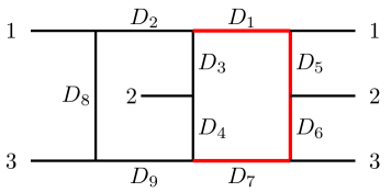
Figure 11: The auxiliary Topology diagram for N${}_{\text{II}}$ as defined in Eq. 4.2. Propagators marked in red are massive.

The second non-planar topology, and most intricate one, corresponds to diagrams with three massive vector bosons and has the following propagator structure

$$I^{\text{N}_{\text{II}}}_{a_{1}\dots a_{9}}=\left(\frac{(-s^{\epsilon})}{\Gamma(\epsilon)}\right)^{2}\int\frac{d^{d}\ell_{1}}{(2\pi)^{d}}\frac{d^{d}\ell_{2}}{(2\pi)^{d}}\frac{1}{D_{1}^{a_{1}}D_{2}^{a_{2}}D_{3}^{a_{3}}D_{4}^{a_{4}}D_{5}^{a_{5}}D_{6}^{a_{6}}D_{7}^{a_{7}}D_{8}^{a_{8}}D_{9}^{a_{9}}},$$ (80)

with:

$$D_{1}=\ell_{1}^{2}-M_{W}^{2}, D_{2}=\ell_{2}^{2}, D_{3}=(\ell_{1}+\ell_{2})^{2},$$

$$D_{4}=(\ell_{1}+\ell_{2}-p_{2})^{2}, D_{5}=(\ell_{1}-p_{1})^{2}-M_{W}^{2}, D_{6}=(\ell_{1}-p_{1}-p_{2})^{2}-M_{W}^{2},$$

$$D_{7}=(\ell_{1}-p_{1}-p_{2}-p_{3})^{2}-M_{W}^{2}, D_{8}=(\ell_{2}+p_{1})^{2}, D_{9}=(\ell_{2}+p_{1}+p_{3})^{2}.$$ (81)

These propagators form an auxiliary topology which is presented in Fig. 11.

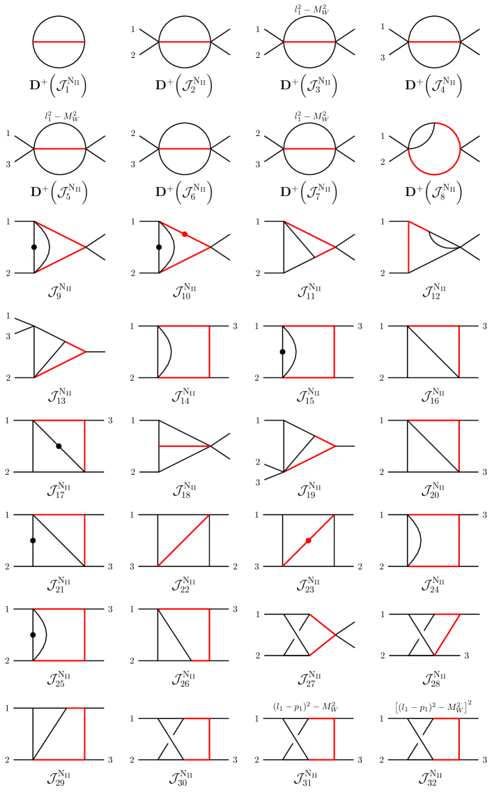
Figure 16: Master integrals for topology N${}_{\text{II}}$. Dotted propagators have higher power of the respective denominator, while red propagators are massive.

After reduction the Feynman diagrams can be expressed in terms of 32 MI’s. Our starting point is the following list of integrals (these are also presented in Fig. 16):

$$\mathcal{J}_{1} ={\bf{D}}^{-}(I^{\text{N}_{\text{II}}}_{111000000}), \mathcal{J}_{2} ={\bf{D}}^{-}(I^{\text{N}_{\text{II}}}_{011001000}), \mathcal{J}_{3} ={\bf{D}}^{-}(I^{\text{N}_{\text{II}}}_{(-1)11001000}),$$

$$\mathcal{J}_{4} ={\bf{D}}^{-}(I^{\text{N}_{\text{II}}}_{010100100}), \mathcal{J}_{5} ={\bf{D}}^{-}(I^{\text{N}_{\text{II}}}_{(-1)10100100}), \mathcal{J}_{6} ={\bf{D}}^{-}(I^{\text{N}_{\text{II}}}_{001000110}),$$

$$\mathcal{J}_{7} ={\bf{D}}^{-}(I^{\text{N}_{\text{II}}}_{(-1)01000110}), \mathcal{J}_{8} ={\bf{D}}^{-}(I^{\text{N}_{\text{II}}}_{111001000}), \mathcal{J}_{9} =I^{\text{N}_{\text{II}}}_{110201000},$$

$$\mathcal{J}_{10} =I^{\text{N}_{\text{II}}}_{210201000} \mathcal{J}_{11} =I^{\text{N}_{\text{II}}}_{111101000}, \mathcal{J}_{12} =I^{\text{N}_{\text{II}}}_{111011000},$$

$$\mathcal{J}_{13} =I^{\text{N}_{\text{II}}}_{111100100}, \mathcal{J}_{14} =I^{\text{N}_{\text{II}}}_{110101100}, \mathcal{J}_{15} =I^{\text{N}_{\text{II}}}_{110201100},$$

$$\mathcal{J}_{16} =I^{\text{N}_{\text{II}}}_{011101100}, \mathcal{J}_{17} =I^{\text{N}_{\text{II}}}_{012101100}, \mathcal{J}_{18} =I^{\text{N}_{\text{II}}}_{111100010},$$

$$\mathcal{J}_{19} =I^{\text{N}_{\text{II}}}_{111000110}, \mathcal{J}_{20} =I^{\text{N}_{\text{II}}}_{101100110}, \mathcal{J}_{21} =I^{\text{N}_{\text{II}}}_{102100110},$$

$$\mathcal{J}_{22} =I^{\text{N}_{\text{II}}}_{011100110}, \mathcal{J}_{23} =I^{\text{N}_{\text{II}}}_{011100210}, \mathcal{J}_{24} =I^{\text{N}_{\text{II}}}_{101001110},$$

$$\mathcal{J}_{25} =I^{\text{N}_{\text{II}}}_{102001110}, \mathcal{J}_{26} =I^{\text{N}_{\text{II}}}_{111101100}, \mathcal{J}_{27} =I^{\text{N}_{\text{II}}}_{111101010},$$

$$\mathcal{J}_{28} =I^{\text{N}_{\text{II}}}_{111100110}, \mathcal{J}_{29} =I^{\text{N}_{\text{II}}}_{111001110}, \mathcal{J}_{30} =I^{\text{N}_{\text{II}}}_{111101110},$$

$$\mathcal{J}_{31} =I^{\text{N}_{\text{II}}}_{1111(-1)1110}, \mathcal{J}_{32} =I^{\text{N}_{\text{II}}}_{1111(-2)1110}.$$ (82)

Here the dimension shifting operator is defined as

$${\bf{D}}^{-}(I^{\text{N}_{\text{II}}}_{a_{1}\dots a_{9}}) = \bigg{(}(a_{1}\mathbf{1}^{+}+a_{5}\mathbf{5}^{+}+a_{6}\mathbf{6}^{+}+a_{7}\mathbf{7}^{+})(a_{2}\mathbf{2}^{+}+a_{8}\mathbf{8}^{+}+a_{9}\mathbf{9}^{+})$$ (83)

$$+(a_{3}\mathbf{3}^{+}+a_{4}\mathbf{4}^{+})(\sum_{j\neq 3,4}\,a_{j}{\mathbf{j}^{+}})\bigg{)}I^{\text{N}_{\text{II}}}_{a_{1}\dots a_{9}}.$$

We proceed as in the earlier sections, first we render each integral dimensionless via the following scaling

$$\mathcal{F}_{X}=\epsilon^{2}\;s^{\alpha}\mathcal{J}_{X}.$$ (84)

Where $\alpha$ is defined for $\mathcal{J}_{X}=f(I^{\text{N}_{\text{II}}}_{a_{1}\dots a_{9}})$ as $(\sum{a_{i}})-4$. We then write a canonical basis in terms of our original integrals and the following dimensionless ratios

$$x=-\frac{p_{1}\cdot p_{3}}{p_{1}\cdot p_{2}},\quad{\rm{and}}\quad y=\frac{M_{W}^{2}}{2p_{1}\cdot p_{2}}.$$ (85)

Given the restriction that both photons must be radiated from the $W$ bosons all permutations of external photons and gluons result in $x>0$ and $y>0$. Finally, in terms of these variables we construct the following canonical basis:

$$\mathcal{G}^{\text{N}_{\text{II}}}_{1}=y\mathcal{F}_{1}, \mathcal{G}^{\text{N}_{\text{II}}}_{2}=\left(1-y\right)\mathcal{F}_{2}, \mathcal{G}^{\text{N}_{\text{II}}}_{3}=\mathcal{F}_{3}+\mathcal{F}_{2},$$

$$\mathcal{G}^{\text{N}_{\text{II}}}_{4}=\left(x+y\right)\mathcal{F}_{4}, \mathcal{G}^{\text{N}_{\text{II}}}_{5}=\mathcal{F}_{5}+y\mathcal{F}_{4}, \mathcal{G}^{\text{N}_{\text{II}}}_{6}=\left(-1+x-y\right)\mathcal{F}_{6},$$

$$\mathcal{G}^{\text{N}_{\text{II}}}_{7}=\mathcal{F}_{7}-\left(2-2x+y\right)\mathcal{F}_{6}, \mathcal{G}^{\text{N}_{\text{II}}}_{8}=\sqrt{r_{1}}\left(y\mathcal{F}_{8}+\mathcal{F}_{2}\right), \mathcal{G}^{\text{N}_{\text{II}}}_{9}=\epsilon\,\mathcal{F}_{9},$$

$$\mathcal{G}^{\text{N}_{\text{II}}}_{10}=\sqrt{r_{1}}\left(y\mathcal{F}_{10}+\frac{3\epsilon}{2}\mathcal{F}_{9}\right), \mathcal{G}^{\text{N}_{\text{II}}}_{11}=\epsilon^{2}\mathcal{F}_{11}, \mathcal{G}^{\text{N}_{\text{II}}}_{12}=\epsilon\,(1-2\epsilon)\mathcal{F}_{12},$$

$$\mathcal{G}^{\text{N}_{\text{II}}}_{13}=\epsilon^{2}x\;\mathcal{F}_{13}, \mathcal{G}^{\text{N}_{\text{II}}}_{14}=\epsilon(2\epsilon-1)\,\mathcal{F}_{14}, \mathcal{G}^{\text{N}_{\text{II}}}_{15}=\epsilon\,\sqrt{r_{2}}\,\mathcal{F}_{15},$$

$$\mathcal{G}^{\text{N}_{\text{II}}}_{16}=\epsilon^{2}\,(x-1)\;\mathcal{F}_{16},$$

$$\mathcal{G}^{\text{N}_{\text{II}}}_{17}=\mathrlap{(1+\epsilon)\frac{(1-x)(xy-x-y)}{x}\mathcal{F}_{17}-\frac{1}{4x^{2}}\bigg{(}2(x+y-x^{2}y)\mathcal{G}^{\text{N}_{\text{II}}}_{1}-2xy(-1+x)\mathcal{G}^{\text{N}_{\text{II}}}_{2}}$$

$$\hskip 30.0pt\mathrlap{+3xy(x-1)\mathcal{G}^{\text{N}_{\text{II}}}_{3}+4(x+y-xy)\mathcal{G}^{\text{N}_{\text{II}}}_{4}-6(x+y-xy)\mathcal{G}^{\text{N}_{\text{II}}}_{5}\bigg{)},}$$

$$\mathcal{G}^{\text{N}_{\text{II}}}_{18}=\epsilon^{2}\mathcal{F}_{18}, \mathcal{G}^{\text{N}_{\text{II}}}_{19}=\epsilon^{2}\,(1-x)\;\mathcal{F}_{19}, \mathcal{G}^{\text{N}_{\text{II}}}_{20}=\epsilon^{2}x\mathcal{F}_{20},$$

$$\mathcal{G}^{\text{N}_{\text{II}}}_{21}=\mathrlap{(1+\epsilon)(1-x+xy)x\mathcal{F}_{21}+\frac{x}{4(1-x)}\bigg{(}2(1+x(y-1)-2y)\mathcal{G}_{1}}$$

$$\hskip 30.0pt\mathrlap{+(x-1)(y-1)(2\mathcal{G}_{2}-3\mathcal{G}_{3})-8y\mathcal{G}_{6}+6y\mathcal{G}_{7}\bigg{)},}$$

$$\mathcal{G}^{\text{N}_{\text{II}}}_{22}=\epsilon^{2}\,\mathcal{F}_{22}, \mathcal{G}^{\text{N}_{\text{II}}}_{23}=\epsilon\,(x-x^{2}+y)\mathcal{F}_{23}, \mathcal{G}^{\text{N}_{\text{II}}}_{24}=\epsilon(2\epsilon-1)\mathcal{F}_{24},$$

$$\mathcal{G}^{\text{N}_{\text{II}}}_{25}=\epsilon\,\sqrt{r_{3}}\,\mathcal{F}_{25}, \mathcal{G}^{\text{N}_{\text{II}}}_{26}=\epsilon^{2}\,\sqrt{r_{4}}\,\mathcal{F}_{26}, \mathcal{G}^{\text{N}_{\text{II}}}_{27}=\epsilon^{2}\,\sqrt{r_{1}}\,\mathcal{F}_{27},$$

$$\mathcal{G}^{\text{N}_{\text{II}}}_{28}=\epsilon^{2}\,\sqrt{r_{5}}\,\mathcal{F}_{28}, \mathcal{G}^{\text{N}_{\text{II}}}_{29}=\epsilon^{2}\,\sqrt{r_{6}}\,\mathcal{F}_{29},$$ (86)

the 7-propagator family is defined as follows:

$$\mathcal{G}^{\text{N}_{\text{II}}}_{30}= -2\epsilon^{2}\bigg{(}2(x-1)\mathcal{F}_{28}+(1-x-2y+4xy)\mathcal{F}_{30}+\mathcal{F}_{31}\bigg{)},$$

$$\mathcal{G}^{\text{N}_{\text{II}}}_{31}= -\epsilon^{2}\,\frac{\sqrt{r_{1}}}{2}\bigg{(}2(x-1)\mathcal{F}_{28}+(1-x)\mathcal{F}_{30}+(1-2x)\mathcal{F}_{31}\bigg{)},$$

$$\mathcal{G}^{\text{N}_{\text{II}}}_{32}= \epsilon^{2}(y\mathcal{F}_{30}+\mathcal{F}_{31}+\mathcal{F}_{32})+\frac{1}{8x}(15\mathcal{G}^{\text{N}_{\text{II}}}_{1}+8\mathcal{G}^{\text{N}_{\text{II}}}_{2}-8\mathcal{G}^{\text{N}_{\text{II}}}_{3}+10\mathcal{G}^{\text{N}_{\text{II}}}_{4}-17\mathcal{G}^{\text{N}_{\text{II}}}_{5}$$

$$+4\mathcal{G}^{\text{N}_{\text{II}}}_{6}-4\mathcal{G}^{\text{N}_{\text{II}}}_{7}-24\mathcal{G}^{\text{N}_{\text{II}}}_{13}-12\mathcal{G}^{\text{N}_{\text{II}}}_{16}-2\mathcal{G}^{\text{N}_{\text{II}}}_{17}+8\mathcal{G}^{\text{N}_{\text{II}}}_{18}-8\mathcal{G}^{\text{N}_{\text{II}}}_{19}+20\mathcal{G}^{\text{N}_{\text{II}}}_{20}$$

$$+2\mathcal{G}^{\text{N}_{\text{II}}}_{21}-24\mathcal{G}^{\text{N}_{\text{II}}}_{22}-8\mathcal{G}^{\text{N}_{\text{II}}}_{23}).$$ (87)

Six non-rational roots appear in the integrals, defined via

$$r_{1}=1-4y r_{2}=x^{2}(1-4y)+2xy+y^{2}$$

$$r_{3}=x^{2}(1-4y)+x(6y-2)+(y-1)^{2} r_{4}=-x\left(4xy-x-4y\right)$$

$$r_{5}=xy\left(x-1\right) r_{6}=-(x-1)(x(4y-1)+1).$$ (88)

The basis integrals and resulting differential equations contain non-rational terms, several of which can be rationalized by an appropriate change of variables. In total there are 6 roots which appear for this topology, shown in Eq. 4.2 and not all of the roots can be simultaneously rationalized. One must therefore make a choice regarding which roots to rationalize to put the set of equations in a form most amenable for a solution in terms of Chen iterated integrals. Since it enters into many of the differential equations $\sqrt{r_{1}}$ is clearly of form which is desirable to rationalize. Since we are interested in solving in the physical region $y>0$ and the behavior of the MI’s depends on whether one evaluates the integral above threshold $(s>4M_{W}^{2}\implies y<1/4$), or below $(s\leq 4M_{W}^{2}\implies y\geq 1/4$), we divide the phase space into relevant regions and introduce the following variable transformations

$${\rm{Region\;\;A}}: s>4M_{W}^{2}, x\in[0,1], y=\frac{z_{A}}{2}\left(1-\frac{z_{A}}{2}\right)$$ (89)

$${\rm{Region\;\;B}}: s\leq 4M_{W}^{2}, x\in[0,1], y=\frac{1-2z_{B}+z_{B}^{2}}{4z_{B}^{2}}.$$ (90)

With $z_{A}\in(0,1]$ and $z_{B}\in[0,1]$. After implementing these transformations the following integrals $\mathcal{G}^{\text{N}_{\text{III}}}_{1-13}$, $\mathcal{G}^{\text{N}_{\text{III}}}_{16-23}$ and $\mathcal{G}^{\text{N}_{\text{III}}}_{27}$ are entirely rational and may therefore be written in terms of GPLs. We evaluate the remaining MIs as Chen-iterated integrals, for which we need to determine boundary solutions. We do so by following the same procedure as for the planar topology discussed in section 3.3, we solve the differential equation in $z_{j}$ at special points in $x$, namely

$$\lim_{x\rightarrow 0}\left(\frac{\partial\mathcal{G}^{\text{N}_{\text{III}}}_{j}}{\partial z_{X}}\right)\quad{\rm{and}}\quad\lim_{x\rightarrow 1}\left(\frac{\partial\mathcal{G}^{\text{N}_{\text{III}}}_{j}}{\partial z_{X}}\right),$$ (91)

with $X=A,B$ appropriately. Each of the roots presented in equation 4.2 ether vanish in these limits or are rationalized entirely by the variables change $y\rightarrow z_{X}$ and therefore the solution may be entirely determined in terms of GPLs. These boundary solutions can be further uniquely fixed by inspecting by taking the decoupling limit $z_{B}\rightarrow 0$, region A boundary points can then be obtained via analytic continuation and matching of the region B solutions.

In order to demonstrate the flexibility of our solutions we present results for the most complicated 7-propagator integrals $\mathcal{G}^{\text{N}_{\text{II}}}_{30-32}$ in Figs. 12-15. Specifically Figs.12, and 14 show the dependence of the loop integrals on $x$ as $z$ is held fixed in region $A$ and $B$ respectively. Figs. 13) and 15 alternatively show the dependence of the integrals on $z$ as $x$ is constant. On each figure a comparison point is shown which shows the result obtained using the numerical package AMFLow, the two being in perfect agreement.

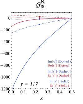
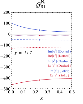
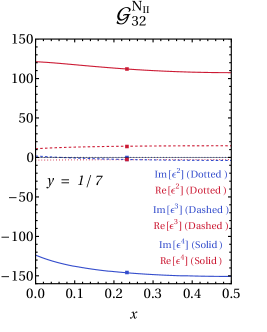
Figure 12: Coefficients of the $\epsilon^{i}$ terms (where $i=2,3,4$) in the expansion of the three 7 point integrals $\mathcal{G}^{\text{N}_{\text{II}}}_{30}$, $\mathcal{G}^{\text{N}_{\text{II}}}_{31}$, and $\mathcal{G}^{\text{N}_{\text{II}}}_{32}$. Here $y=1/7$ and $x$ is varied in the region $u<t$ (Region A, as defined in Eq. 89). Red and blue squares represent the real and imaginary part, respectively, of independent evaluation using AMFlow.

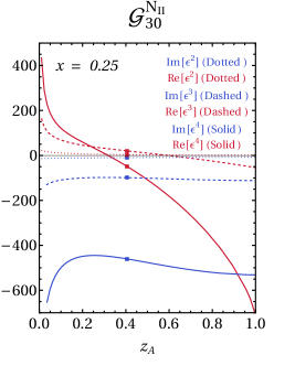
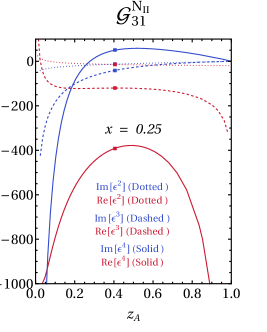
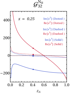
Figure 13: Coefficients of the $\epsilon^{i}$ terms (where $i=2,3,4$) in the expansion of the three 7 point integrals $\mathcal{G}^{\text{N}_{\text{II}}}_{30}$, $\mathcal{G}^{\text{N}_{\text{II}}}_{31}$, and $\mathcal{G}^{\text{N}_{\text{II}}}_{32}$. Here $x=0.25$ and $y$ is varied in the region $y<1/4$ (Region A, as defined in Eq. 89). Red and blue squares represent the real and imaginary part, respectively, of independent evaluation using AMFlow.

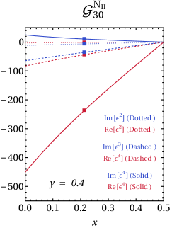
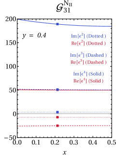
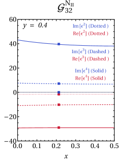
Figure 14: Coefficients of the $\epsilon^{i}$ terms (where $i=2,3,4$) in the expansion of the three 7 point integrals $\mathcal{G}^{\text{N}_{\text{II}}}_{30}$, $\mathcal{G}^{\text{N}_{\text{II}}}_{31}$, and $\mathcal{G}^{\text{N}_{\text{II}}}_{32}$. Here $y=0.4$ and $x$ is varied in the region $u<t$ (Region B, as defined in Eq. 90). Red and blue squares represent the real and imaginary part, respectively, of independent evaluation using AMFlow.

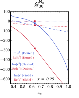
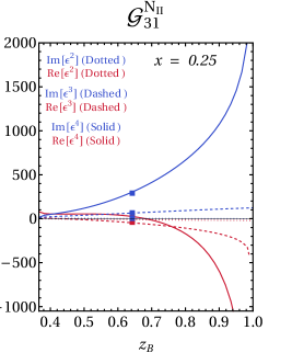
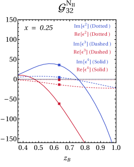
Figure 15: Coefficients of the $\epsilon^{i}$ terms (where $i=2,3,4$) in the expansion of the three 7 point integrals $\mathcal{G}^{\text{N}_{\text{II}}}_{30}$,$\mathcal{G}^{\text{N}_{\text{II}}}_{31}$, and $\mathcal{G}^{\text{N}_{\text{II}}}_{32}$. Here $x=0.25$ and and $y$ is varied in the region $y>1/4$ (Region B, as defined in Eq. 90). Red and blue squares represent the real and imaginary part, respectively, of independent evaluation using AMFlow.

5 Conclusions

In this paper we have presented the calculation of the Master Integrals required for the evaluation of electroweak corrections to the amplitude for $gg\rightarrow\gamma\gamma$ for the cases in which the closed loop of fermions corresponds to the first two generations. We solved for the MI’s using a differential equation method, specifically by choosing a set of MI’s which obeyed a differential equation in canonical form (in which the $\epsilon$ series factorizes from the kinematics in the differential equation) we were able to solve our integrals using iterated integrals.

We are able to classify our integrals based on the flow of the massive vector bosons through the diagrams. The situation in which there is no massive bosons (i.e. QED corrections) is well known and we did not discuss the answer in detail here. Topologies for which there is a single massive boson in the loop was also straightforward, there are only planar topologies with no issues regarding non-rational letters, such that the answer could be written entirely in terms of GPL solutions. For topologies with two massive vector bosons there are planar and non-planar topologies to consider. The planar topologies with two massive bosons are similar to those with one, in that they are readily written entirely in-terms of GPL solutions. For non-planar topologies non-rational letters initially appear in the alphabet, however by an appropriate variable change we were able to rationalize the roots such that a GPL solution was obtained for all two $W$ boson topologies.

Finally the most complicated topologies we had to consider came from diagrams which contain three massive vector bosons. Again here there are both planar and non-planar topologies to consider. The increased number of internal massive lines lead to a proliferation of non-rational letters in the alphabet of the differential equations. In order to solve the differential equations in this instance we used a mixed Goncharov-Chen approach. By writing the non-rational contributions as Chen-iterated integrals we were able to define as solution as a two-parameter integral when expanded up to weight 4.

We evaluated our integrals in all required regions of kinematic phase space for physical scattering. We checked all of our solutions against public numerical packages, finding prefect agreement, in general our analytic solutions were orders of magnitude quicker than the numerical checks, and should be amenable to implementation into a Monte Carlo generator for subsequent phenomenological analysis, which we will pursue in a subsequent publication.

Appendix A Numerical Tables

A.1 Topology P${}_{\text{I}}$

Integral	$\epsilon^{0}$	$\epsilon^{1}$	$\epsilon^{2}$	$\epsilon^{3}$	$\epsilon^{4}$
$\mathcal{G}^{\text{P}_{\text{I}}}_{1}$	-1	0	-3.28987	2.40411	-9.74091
$\mathcal{G}^{\text{P}_{\text{I}}}_{2}$	2	-1.79943 + 6.28319$i$	-12.35 - 5.65307$i$	6.78877 - 18.1278$i$	18.5363 + 2.72968$i$
$\mathcal{G}^{\text{P}_{\text{I}}}_{3}$	-1	1.51073 - 12.5664$i$	59.9621 + 2.02519$i$	48.2216 + 169.018$i$	-300.438 + 290.282$i$
$\mathcal{G}^{\text{P}_{\text{I}}}_{4}$	1	-0.755365 + 6.28319$i$	-25.9088 + 1.81394$i$	-31.3687 - 73.4063$i$	129.896 - 137.865$i$
$\mathcal{G}^{\text{P}_{\text{I}}}_{5}$	2	-1.61875	-2.63478	-2.32223	-2.02061
$\mathcal{G}^{\text{P}_{\text{I}}}_{6}$	-1	4.71031	-4.96941	14.0924	-25.3592
$\mathcal{G}^{\text{P}_{\text{I}}}_{7}$	0	1.17758	-1.20438	3.00559	-6.20665
$\mathcal{G}^{\text{P}_{\text{I}}}_{8}$	0	0	0	2.46908 + 5.27231$i$	-10.8039 + 8.64876$i$
$\mathcal{G}^{\text{P}_{\text{I}}}_{9}$	0	0	-0.561726 - 3.89856$i$	8.7916 - 5.05245$i$	6.3134 + 0.0902883$i$
$\mathcal{G}^{\text{P}_{\text{I}}}_{10}$	0	0	0	-4.11017	-1.80935
$\mathcal{G}^{\text{P}_{\text{I}}}_{11}$	0	0	2.63271	2.30232	8.96751
$\mathcal{G}^{\text{P}_{\text{I}}}_{12}$	4	-6.47499	-7.91879	-0.758835	6.37784
$\mathcal{G}^{\text{P}_{\text{I}}}_{13}$	0	0	0	0.799872 - 4.00077$i$	14.1684 - 0.891901$i$
$\mathcal{G}^{\text{P}_{\text{I}}}_{14}$	0	0	-1.56899	-1.67582	-5.31164
$\mathcal{G}^{\text{P}_{\text{I}}}_{15}$	-4	3.41818 - 6.28319$i$	14.9929 + 5.08544$i$	-3.5778 + 18.0579$i$	-16.4178 - 1.15688$i$
$\mathcal{G}^{\text{P}_{\text{I}}}_{16}$	1	-1.18706 + 3.14159$i$	-13.1838 + 1.19078$i$	-18.7334 - 36.3309$i$	63.9675 - 71.8708$i$
$\mathcal{G}^{\text{P}_{\text{I}}}_{17}$	0	0.377683 - 3.14159$i$	16.721 + 4.46229$i$	10.4971 + 59.0473$i$	-114.05 + 88.9521$i$
$\mathcal{G}^{\text{P}_{\text{I}}}_{18}$	1	-2.07729 + 3.14159$i$	-7.04912 - 6.526$i$	11.2944 - 8.85682$i$	6.58424 + 9.52116$i$
$\mathcal{G}^{\text{P}_{\text{I}}}_{19}$	0	1.17758	-2.26387 + 3.69947$i$	-9.64506 - 4.79304$i$	2.65821 - 16.1321$i$
$\mathcal{G}^{\text{P}_{\text{I}}}_{20}$	0	0	0.134973 + 0.165281$i$	-0.397866 + 0.589612$i$	-1.62649 + 0.0748837$i$
$\mathcal{G}^{\text{P}_{\text{I}}}_{21}$	0	-1.55526 + 3.14159$i$	-16.1407 - 4.08498$i$	-7.58796 - 56.7198$i$	114.6 - 84.1576$i$
$\mathcal{G}^{\text{P}_{\text{I}}}_{22}$	0	0	0	-4.50119	7.32103
$\mathcal{G}^{\text{P}_{\text{I}}}_{23}$	-1	3.12948 - 12.5664$i$	55.1793 + 0.0852468$i$	63.663 + 169.72$i$	-291.552 + 326.643$i$
$\mathcal{G}^{\text{P}_{\text{I}}}_{24}$	1	-2.37411 + 6.28319$i$	-26.0172 + 2.94919$i$	-29.6303 - 71.2136$i$	131.079 - 143.964$i$
$\mathcal{G}^{\text{P}_{\text{I}}}_{25}$	0	0	0	0	13.308 + 2.2413$i$

Table 1: Numerical results for the 25 integrals of Topology $\text{P}_{\text{I}}$. The integrals are evaluated in Region A, as defined in Eq.31, at the sample point $x=-2.4589$ and $y=2.2465$.

Integral	$\epsilon^{0}$	$\epsilon^{1}$	$\epsilon^{2}$	$\epsilon^{3}$	$\epsilon^{4}$
$\mathcal{G}^{\text{P}_{\text{I}}}_{1}$	-1	0	-3.28987	2.40411	-9.74091
$\mathcal{G}^{\text{P}_{\text{I}}}_{2}$	2	-2.90079	-1.18622	-1.05366	-0.988206
$\mathcal{G}^{\text{P}_{\text{I}}}_{3}$	-1	6.64417	-10.5138	20.7927	-42.9302
$\mathcal{G}^{\text{P}_{\text{I}}}_{4}$	1	-3.32209	4.4271	-10.1262	19.169
$\mathcal{G}^{\text{P}_{\text{I}}}_{5}$	2	-2.40949	-1.83846	-1.42764	-1.2897
$\mathcal{G}^{\text{P}_{\text{I}}}_{6}$	-1	5.86772	-7.96034	17.5021	-35.0958
$\mathcal{G}^{\text{P}_{\text{I}}}_{7}$	0	1.46693	-2.213	4.18951	-9.3411
$\mathcal{G}^{\text{P}_{\text{I}}}_{8}$	0	0	0	-6.12631	0.17907
$\mathcal{G}^{\text{P}_{\text{I}}}_{9}$	0	0	3.70427	1.46967	12.2132
$\mathcal{G}^{\text{P}_{\text{I}}}_{10}$	0	0	0	-5.27174	-0.802495
$\mathcal{G}^{\text{P}_{\text{I}}}_{11}$	0	0	3.26041	1.89421	10.7715
$\mathcal{G}^{\text{P}_{\text{I}}}_{12}$	4	-9.63794	-1.54824	3.14894	5.10092
$\mathcal{G}^{\text{P}_{\text{I}}}_{13}$	0	0	0	3.00395	-0.423949
$\mathcal{G}^{\text{P}_{\text{I}}}_{14}$	0	0	-2.09076	-1.73255	-6.52823
$\mathcal{G}^{\text{P}_{\text{I}}}_{15}$	-4	5.31028	12.9546	0.421382	-10.2771
$\mathcal{G}^{\text{P}_{\text{I}}}_{16}$	1	-2.86579	-0.824244	-1.5515	7.01
$\mathcal{G}^{\text{P}_{\text{I}}}_{17}$	0	1.66104	-5.0445	-8.01612	-4.02791
$\mathcal{G}^{\text{P}_{\text{I}}}_{18}$	1	-2.91732	-0.434013	-2.49897	7.90258
$\mathcal{G}^{\text{P}_{\text{I}}}_{19}$	0	1.46693	-4.34063	-6.67956	-3.65615
$\mathcal{G}^{\text{P}_{\text{I}}}_{20}$	0	0	-2.77842	2.09681	-4.45944
$\mathcal{G}^{\text{P}_{\text{I}}}_{21}$	0	-3.12797	-1.29177	5.28593	10.2361
$\mathcal{G}^{\text{P}_{\text{I}}}_{22}$	0	0	0	-4.90792	10.9452
$\mathcal{G}^{\text{P}_{\text{I}}}_{23}$	-1	9.05366	6.27915	-28.4251	-44.0975
$\mathcal{G}^{\text{P}_{\text{I}}}_{24}$	1	-5.73157	-8.58628	3.77865	20.6685
$\mathcal{G}^{\text{P}_{\text{I}}}_{25}$	0	0	0	0	-10.6725

Table 2: Numerical results for the 25 integrals of Topology $\text{P}_{\text{I}}$. The integrals are evaluated in Region B, as defined in Eq.32, at the sample point $x=4.2648$ and $y=3.3359$.

Integral	$\epsilon^{0}$	$\epsilon^{1}$	$\epsilon^{2}$	$\epsilon^{3}$	$\epsilon^{4}$
$\mathcal{G}^{\text{P}_{\text{I}}}_{1}$	-1	0	-3.28987	2.40411	-9.74091
$\mathcal{G}^{\text{P}_{\text{I}}}_{2}$	2	2.11744	-2.16898	-7.89571	-11.7001
$\mathcal{G}^{\text{P}_{\text{I}}}_{3}$	-1	1.19122	-2.07511	6.89876	-8.20121
$\mathcal{G}^{\text{P}_{\text{I}}}_{4}$	1	-0.595611	2.36178	-4.88683	7.75393
$\mathcal{G}^{\text{P}_{\text{I}}}_{5}$	2	-0.272381 + 6.28319$i$	-13.1409 - 0.855709$i$	-3.01688 - 20.6126$i$	20.0146 - 12.293$i$
$\mathcal{G}^{\text{P}_{\text{I}}}_{6}$	-1	-7.69934 - 12.5664$i$	33.7392 - 99.3198$i$	466.546 - 227.039$i$	1909.94 + 576.108$i$
$\mathcal{G}^{\text{P}_{\text{I}}}_{7}$	0	-1.92483 - 3.14159$i$	10.2813 - 24.616$i$	119.158 - 54.2128$i$	487.629 + 158.085$i$
$\mathcal{G}^{\text{P}_{\text{I}}}_{8}$	0	0	0	-1.1328	-1.95545
$\mathcal{G}^{\text{P}_{\text{I}}}_{9}$	0	0	0.833835	1.83071	4.38072
$\mathcal{G}^{\text{P}_{\text{I}}}_{10}$	0	0	0	1.91488 + 2.89532$i$	-4.23565 + 7.46431$i$
$\mathcal{G}^{\text{P}_{\text{I}}}_{11}$	0	0	-0.81762 - 2.39879$i$	4.23739 - 5.61184$i$	7.33633 - 4.34692$i$
$\mathcal{G}^{\text{P}_{\text{I}}}_{12}$	4	-1.08952 + 25.1327$i$	-91.9679 - 6.84567$i$	5.84432 - 247.118$i$	512.679 - 53.3645$i$
$\mathcal{G}^{\text{P}_{\text{I}}}_{13}$	0	0	0	0.799592	1.66788
$\mathcal{G}^{\text{P}_{\text{I}}}_{14}$	0	0	2.04798 + 0.427855$i$	7.70385 + 5.12304$i$	18.4844 + 28.5217$i$
$\mathcal{G}^{\text{P}_{\text{I}}}_{15}$	-4	-1.84506 - 6.28319$i$	16.7377 - 6.65213$i$	24.1202 + 11.5908$i$	4.44028 + 26.4637$i$
$\mathcal{G}^{\text{P}_{\text{I}}}_{16}$	1	-0.433996 + 3.14159$i$	-7.31466 - 1.36344$i$	0.632443 - 10.1336$i$	8.23075 - 2.35015$i$
$\mathcal{G}^{\text{P}_{\text{I}}}_{17}$	0	0.297806	0.102776 + 0.935584$i$	-1.94227 + 0.707591$i$	-2.28442 - 2.17101$i$
$\mathcal{G}^{\text{P}_{\text{I}}}_{18}$	1	2.98355 + 3.14159$i$	-5.23195 + 28.7978$i$	-120.856 + 94.254$i$	-615.173 - 13.1543$i$
$\mathcal{G}^{\text{P}_{\text{I}}}_{19}$	0	-1.92483 - 3.14159$i$	8.24341 - 27.9421$i$	138.436 - 83.0437$i$	669.262 + 82.9275$i$
$\mathcal{G}^{\text{P}_{\text{I}}}_{20}$	0	0	1.33007 + 0.292072$i$	4.78264 + 3.48455$i$	10.9039 + 19.2933$i$
$\mathcal{G}^{\text{P}_{\text{I}}}_{21}$	0	1.62703 + 3.14159$i$	-6.83158 + 25.3565$i$	-108.996 + 63.017$i$	-461.856 - 109.585$i$
$\mathcal{G}^{\text{P}_{\text{I}}}_{22}$	0	0	0	-4.051 + 5.1399$i$	-23.0107 - 17.535$i$
$\mathcal{G}^{\text{P}_{\text{I}}}_{23}$	-1	1.4636 - 6.28319$i$	19.281 + 3.27123$i$	-22.1225 + 47.5912$i$	-161.918 - 57.2343$i$
$\mathcal{G}^{\text{P}_{\text{I}}}_{24}$	1	-0.867992 + 6.28319$i$	-20.1271 - 2.19925$i$	16.3575 - 49.4622$i$	147.355 + 46.4819$i$
$\mathcal{G}^{\text{P}_{\text{I}}}_{25}$	0	0	0	0	2.21507 - 3.01982$i$

Table 3: Numerical results for the 25 integrals of Topology $\text{P}_{\text{I}}$. The integrals are evaluated in Region C, as defined in Eq.33, at the sample point $x=0.3469$ and $y=-1.1459$.

A.2 Topology P${}_{\text{II}}$

Integral	$\epsilon^{0}$	$\epsilon^{1}$	$\epsilon^{2}$	$\epsilon^{3}$	$\epsilon^{4}$
$\mathcal{G}^{\text{P}_{\text{II}}}_{1}$	-1	0	-3.28987	2.40411	-9.74091
$\mathcal{G}^{\text{P}_{\text{II}}}_{2}$	2	-2.28832 + 6.28319$i$	-11.8504 - 7.18896$i$	9.74903 - 16.5582$i$	16.5125 + 6.97674$i$
$\mathcal{G}^{\text{P}_{\text{II}}}_{3}$	-1	3.04285 - 12.5664$i$	57.3151 + 16.6707$i$	-17.3517 + 160.478$i$	-324.915 + 104.559$i$
$\mathcal{G}^{\text{P}_{\text{II}}}_{4}$	1	-1.52142 + 6.28319$i$	-24.7256 - 4.74086$i$	-2.66226 - 70.1134$i$	142.408 - 56.4524$i$
$\mathcal{G}^{\text{P}_{\text{II}}}_{5}$	-1	3.57274	-2.9985	11.8091	-17.5852
$\mathcal{G}^{\text{P}_{\text{II}}}_{6}$	0	0.893186	-0.483293	2.25504	-3.68858
$\mathcal{G}^{\text{P}_{\text{II}}}_{7}$	2	-0.73331	-3.15543	-3.61841	-3.32713
$\mathcal{G}^{\text{P}_{\text{II}}}_{8}$	-1	1.14416 - 3.14159$i$	6.30304 + 8.05758$i$	-17.9535 + 6.24897$i$	1.00202 - 13.4629$i$
$\mathcal{G}^{\text{P}_{\text{II}}}_{9}$	0	0	0	2.58505 + 6.29354$i$	-13.7782 + 8.38369$i$
$\mathcal{G}^{\text{P}_{\text{II}}}_{10}$	0	0	0	-3.07869	-2.32866
$\mathcal{G}^{\text{P}_{\text{II}}}_{11}$	0	0	2.04657	2.45204	7.46877
$\mathcal{G}^{\text{P}_{\text{II}}}_{12}$	0	0	0	1.25399	0.690107
$\mathcal{G}^{\text{P}_{\text{II}}}_{13}$	0	0	0	0	1.47748 + 6.87675$i$
$\mathcal{G}^{\text{P}_{\text{II}}}_{14}$	0	0	-1.90921 + 0.868614$i$	-5.46692 - 3.68129$i$	3.85792 - 9.7775$i$
$\mathcal{G}^{\text{P}_{\text{II}}}_{15}$	1	-2.03734 + 3.14159$i$	-6.64448 - 6.40051$i$	11.301 - 6.40934$i$	1.11419 + 9.26507$i$
$\mathcal{G}^{\text{P}_{\text{II}}}_{16}$	0	0.893186	-1.50524 + 2.80603$i$	-6.69697 - 2.5648$i$	0.724511 - 9.41922$i$
$\mathcal{G}^{\text{P}_{\text{II}}}_{17}$	0	0	0	-1.78682 - 0.918304$i$	0.191481 - 4.36$i$
$\mathcal{G}^{\text{P}_{\text{II}}}_{18}$	0	1.6539 - 3.14159$i$	13.3872 + 3.78675$i$	0.717181 + 41.4859$i$	-81.4212 + 38.7063$i$
$\mathcal{G}^{\text{P}_{\text{II}}}_{19}$	-4	3.02163 - 6.28319$i$	15.6103 + 2.30376$i$	1.39621 + 16.2313$i$	-13.5634 + 6.1045$i$
$\mathcal{G}^{\text{P}_{\text{II}}}_{20}$	1	-1.12737 + 3.14159$i$	-13.0194 + 0.0721714$i$	-13.1936 - 33.9416$i$	59.5314 - 54.4339$i$
$\mathcal{G}^{\text{P}_{\text{II}}}_{21}$	0	0.760712 - 3.14159$i$	16.0159 + 7.11679$i$	1.74473 + 59.7822$i$	-117.48 + 68.6029$i$
$\mathcal{G}^{\text{P}_{\text{II}}}_{22}$	0	0	0	0	-2.90866
$\mathcal{G}^{\text{P}_{\text{II}}}_{23}$	0	0	1.11227	-1.88646 + 2.35627$i$	-7.16027 - 7.04561$i$
$\mathcal{G}^{\text{P}_{\text{II}}}_{24}$	0	0	-2.28707 - 3.59448$i$	10.1684 - 9.94568$i$	42.9927 + 10.1081$i$

Table 4: Numerical results for the 24 integrals of topology P${}_{\text{II}}$. The integrals are evaluated in Region A, as defined in Eq. 42, at the sample point $x=-3.1398$ and $y=1.4429$.

Integral	$\epsilon^{0}$	$\epsilon^{1}$	$\epsilon^{2}$	$\epsilon^{3}$	$\epsilon^{4}$
$\mathcal{G}^{\text{P}_{\text{II}}}_{1}$	-1	0	-3.28987	2.40411	-9.74091
$\mathcal{G}^{\text{P}_{\text{II}}}_{2}$	2	-2.11967	-2.16661	-1.71833	-1.51706
$\mathcal{G}^{\text{P}_{\text{II}}}_{3}$	-1	5.42942	-6.71206	16.0318	-31.168
$\mathcal{G}^{\text{P}_{\text{II}}}_{4}$	1	-2.71471	3.11478	-8.67794	15.0184
$\mathcal{G}^{\text{P}_{\text{II}}}_{5}$	-1	5.79661	-7.7483	17.2464	-34.4366
$\mathcal{G}^{\text{P}_{\text{II}}}_{6}$	0	1.44915	-2.1431	4.10035	-9.12827
$\mathcal{G}^{\text{P}_{\text{II}}}_{7}$	2	-2.36315	-1.89375	-1.47088	-1.32327
$\mathcal{G}^{\text{P}_{\text{II}}}_{8}$	-1	1.05984	-1.93498	3.59655	-8.04274
$\mathcal{G}^{\text{P}_{\text{II}}}_{9}$	0	0	0	-4.81701	-1.24457
$\mathcal{G}^{\text{P}_{\text{II}}}_{10}$	0	0	0	-5.19666	-0.879496
$\mathcal{G}^{\text{P}_{\text{II}}}_{11}$	0	0	3.22073	1.9269	10.6498
$\mathcal{G}^{\text{P}_{\text{II}}}_{12}$	0	0	0	2.51453	0.542128
$\mathcal{G}^{\text{P}_{\text{II}}}_{13}$	0	0	0	0	-4.41432
$\mathcal{G}^{\text{P}_{\text{II}}}_{14}$	0	0	-1.13211	-2.88739	-4.61031
$\mathcal{G}^{\text{P}_{\text{II}}}_{15}$	1	-2.50899	-1.51831	-2.22401	5.87141
$\mathcal{G}^{\text{P}_{\text{II}}}_{16}$	0	1.44915	-3.67896	-7.591	-5.79339
$\mathcal{G}^{\text{P}_{\text{II}}}_{17}$	0	0	0	3.79314	-1.96722
$\mathcal{G}^{\text{P}_{\text{II}}}_{18}$	0	2.80651	2.27273	-2.99283	-8.27529
$\mathcal{G}^{\text{P}_{\text{II}}}_{19}$	-4	4.48282	13.9448	3.17825	-9.88202
$\mathcal{G}^{\text{P}_{\text{II}}}_{20}$	1	-2.53893	-1.31679	-2.59823	6.14537
$\mathcal{G}^{\text{P}_{\text{II}}}_{21}$	0	1.35735	-3.40245	-6.895	-5.37232
$\mathcal{G}^{\text{P}_{\text{II}}}_{22}$	0	0	0	0	-4.73229
$\mathcal{G}^{\text{P}_{\text{II}}}_{23}$	0	0	2.05698	-1.96362	-6.23
$\mathcal{G}^{\text{P}_{\text{II}}}_{24}$	0	0	1.88618	-1.77268	-5.29583

Table 5: Numerical results for the 24 integrals of topology P${}_{\text{II}}$. The integrals are evaluated in Region B, as defined in Eq. 43, at the sample point $x=2.8859$ and $y=3.2595$.

A.3 Topology P${}_{\text{III}}$

Integral	$\epsilon^{0}$	$\epsilon^{1}$	$\epsilon^{2}$	$\epsilon^{3}$	$\epsilon^{4}$
$\mathcal{G}^{\text{P}_{\text{III}}}_{1}$	-1	0	-3.28987	2.40411	-9.74091
$\mathcal{G}^{\text{P}_{\text{III}}}_{2}$	2	-2.44431 + 6.28319$i$	-11.6658 - 7.67904$i$	10.6662 - 15.9784$i$	15.7162 + 8.24587$i$
$\mathcal{G}^{\text{P}_{\text{III}}}_{3}$	-1	3.4927 - 12.5664$i$	56.2276 + 20.8534$i$	-35.3395 + 155.103$i$	-318.936 + 54.3136$i$
$\mathcal{G}^{\text{P}_{\text{III}}}_{4}$	-1	1.74635 - 6.28319$i$	24.2455 + 6.5872$i$	-5.07237 + 67.9369$i$	-140.401 + 34.7934$i$
$\mathcal{G}^{\text{P}_{\text{III}}}_{5}$	-1	3.96632	-3.57047	12.5279	-20.0835
$\mathcal{G}^{\text{P}_{\text{III}}}_{6}$	0	0.99158	-0.702254	2.48225	-4.50394
$\mathcal{G}^{\text{P}_{\text{III}}}_{7}$	0	0	-0.307202 - 4.65067$i$	11.0493 - 3.93605$i$	3.7623 + 2.02169$i$
$\mathcal{G}^{\text{P}_{\text{III}}}_{8}$	0	0	0	2.61181 + 6.64895$i$	-14.8211 + 8.19906$i$
$\mathcal{G}^{\text{P}_{\text{III}}}_{9}$	0	0. + 2.34235$i$	-6.10326 + 4.37516$i$	-17.7599 - 7.33235$i$	2.81167 - 46.0371$i$
$\mathcal{G}^{\text{P}_{\text{III}}}_{10}$	0	0. - 9.3694$i$	29.4348 - 1.13343$i$	3.56079 + 60.2645$i$	-92.4897 + 30.0229$i$
$\mathcal{G}^{\text{P}_{\text{III}}}_{11}$	0	0	-5.4866	-7.32639	-16.7408
$\mathcal{G}^{\text{P}_{\text{III}}}_{12}$	0	0. + 2.34235$i$	0. + 3.14608$i$	0. + 3.72183$i$	0. - 7.11178$i$
$\mathcal{G}^{\text{P}_{\text{III}}}_{13}$	0	0	0	0	1.37323 + 7.20982$i$
$\mathcal{G}^{\text{P}_{\text{III}}}_{14}$	0	0	-1.91612 + 0.811151$i$	-5.08816 - 3.72197$i$	4.26994 - 8.47007$i$
$\mathcal{G}^{\text{P}_{\text{III}}}_{15}$	1	-2.21374 + 3.14159$i$	-6.4472 - 6.95466$i$	12.457 - 5.75855$i$	-0.0376254 + 10.2821$i$
$\mathcal{G}^{\text{P}_{\text{III}}}_{16}$	0	0.99158	-1.91412 + 3.11514$i$	-7.39861 - 3.52493$i$	2.01986 - 10.6336$i$
$\mathcal{G}^{\text{P}_{\text{III}}}_{17}$	0	0	0	-1.70036 - 0.943653$i$	0.64075 - 4.1616$i$
$\mathcal{G}^{\text{P}_{\text{III}}}_{18}$	0	1.86475 - 3.14159$i$	13.1082 + 5.49979$i$	-5.19227 + 42.2605$i$	-86.9637 + 25.7847$i$
$\mathcal{G}^{\text{P}_{\text{III}}}_{19}$	0	0	0	1.44546	0.713956
$\mathcal{G}^{\text{P}_{\text{III}}}_{20}$	0	0	-2.7433	-1.87382 - 2.77921$i$	-3.45475 - 10.6005$i$
$\mathcal{G}^{\text{P}_{\text{III}}}_{21}$	0	0	-2.7433	1.76327 - 8.61834$i$	17.1739 + 5.53946$i$
$\mathcal{G}^{\text{P}_{\text{III}}}_{22}$	0	0	0	3.12674 - 11.6783$i$	41.65 + 19.2504$i$
$\mathcal{G}^{\text{P}_{\text{III}}}_{23}$	0	0	0	-6.38107 - 5.12545$i$	-0.302294 - 21.7425$i$
$\mathcal{G}^{\text{P}_{\text{III}}}_{24}$	0	0	-2.7433	1.03354	-2.99786
$\mathcal{G}^{\text{P}_{\text{III}}}_{25}$	0	0	3.96819	8.78464	10.3528
$\mathcal{G}^{\text{P}_{\text{III}}}_{26}$	0	0	1.26421	-2.32486 + 2.56903$i$	-7.56341 - 8.62886$i$
$\mathcal{G}^{\text{P}_{\text{III}}}_{27}$	0	0	0	0	5.1483 + 4.05094$i$
$\mathcal{G}^{\text{P}_{\text{III}}}_{28}$	0	0	0	5.88157 + 6.62362$i$	1.72768 + 28.0861$i$
$\mathcal{G}^{\text{P}_{\text{III}}}_{29}$	0	0	3.96819	-5.76835 - 3.55034$i$	-16.7338 - 57.9513$i$
$\mathcal{G}^{\text{P}_{\text{III}}}_{30}$	0	0	0	0	-0.575238 - 0.729338$i$
$\mathcal{G}^{\text{P}_{\text{III}}}_{31}$	0	0	-2.7433	7.57798 - 3.05993$i$	14.1357 + 32.1012$i$
$\mathcal{G}^{\text{P}_{\text{III}}}_{32}$	0	0	0	3.40071 + 1.88731$i$	-4.87662 + 4.78924$i$

Table 6: Numerical results for the 32 integrals of topology P${}_{\text{III}}$. The integrals are evaluated in Region A, as defined in Eq. 54, at the sample point $x=1.69549$ and $y=-3.3945$.

Integral	$\epsilon^{0}$	$\epsilon^{1}$	$\epsilon^{2}$	$\epsilon^{3}$	$\epsilon^{4}$
$\mathcal{G}^{\text{P}_{\text{III}}}_{1}$	-1	0	-3.28987	2.40411	-9.74091
$\mathcal{G}^{\text{P}_{\text{III}}}_{2}$	2	-2.99455 + 6.28319$i$	-10.9176 - 9.40767$i$	13.7763 - 13.6279$i$	12.3492 + 12.3294$i$
$\mathcal{G}^{\text{P}_{\text{III}}}_{3}$	-1	4.97604 - 12.5664$i$	51.6989 + 34.3078$i$	-90.1785 + 129.099$i$	-263.462 - 92.0311$i$
$\mathcal{G}^{\text{P}_{\text{III}}}_{4}$	-1	2.48802 - 6.28319$i$	22.2732 + 12.4501$i$	-28.2614 + 57.4298$i$	-119.079 - 27.3863$i$
$\mathcal{G}^{\text{P}_{\text{III}}}_{5}$	-1	4.92312	-5.44537	14.6137	-27.0022
$\mathcal{G}^{\text{P}_{\text{III}}}_{6}$	0	1.23078	-1.36913	3.18477	-6.73497
$\mathcal{G}^{\text{P}_{\text{III}}}_{7}$	0	0	-0.00936825 - 5.33815$i$	13.0223 - 2.46789$i$	0.329742 + 3.20266$i$
$\mathcal{G}^{\text{P}_{\text{III}}}_{8}$	0	0	0	2.65712 + 8.02212$i$	-18.859 + 7.07761$i$
$\mathcal{G}^{\text{P}_{\text{III}}}_{9}$	0	0.672459 - 3.14159$i$	17.2197 + 0.793569$i$	8.97323 + 49.1711$i$	-100.877 + 54.7732$i$
$\mathcal{G}^{\text{P}_{\text{III}}}_{10}$	0	-2.68983 + 12.5664$i$	-69.4825 - 17.7644$i$	54.1099 - 214.834$i$	487.856 + 80.9159$i$
$\mathcal{G}^{\text{P}_{\text{III}}}_{11}$	0	0	-9.4174 - 4.22518$i$	-10.8032 - 12.0621$i$	-14.9631 - 6.05697$i$
$\mathcal{G}^{\text{P}_{\text{III}}}_{12}$	0	0.672459 - 3.14159$i$	8.50787 - 2.37532$i$	2.60623 + 12.4742$i$	-21.1972 + 20.622$i$
$\mathcal{G}^{\text{P}_{\text{III}}}_{13}$	0	0	0	0	0.912314 + 8.42193$i$
$\mathcal{G}^{\text{P}_{\text{III}}}_{14}$	0	0	-1.9219 + 0.634321$i$	-3.9331 - 3.67257$i$	4.69996 - 4.43151$i$
$\mathcal{G}^{\text{P}_{\text{III}}}_{15}$	1	-2.72806 + 3.14159$i$	-5.56789 - 8.57044$i$	15.7439 - 2.66663$i$	-5.84004 + 12.6208$i$
$\mathcal{G}^{\text{P}_{\text{III}}}_{16}$	0	1.23078	-3.21195 + 3.86661$i$	-8.55908 - 6.55849$i$	6.66695 - 12.2735$i$
$\mathcal{G}^{\text{P}_{\text{III}}}_{17}$	0	0	0	-1.71668 - 1.20926$i$	2.18469 - 4.07839$i$
$\mathcal{G}^{\text{P}_{\text{III}}}_{18}$	0	2.47479 - 3.14159$i$	11.2287 + 10.1168$i$	-21.705 + 38.5434$i$	-85.3521 - 15.0574$i$
$\mathcal{G}^{\text{P}_{\text{III}}}_{19}$	0	0	0	1.96557	0.691136
$\mathcal{G}^{\text{P}_{\text{III}}}_{20}$	0	0	-4.7087 - 2.11259$i$	3.51701 - 13.3845$i$	26.3234 - 8.84441$i$
$\mathcal{G}^{\text{P}_{\text{III}}}_{21}$	0	0	-4.7087 - 2.11259$i$	11.4546 - 17.505$i$	40.7022 + 29.9841$i$
$\mathcal{G}^{\text{P}_{\text{III}}}_{22}$	0	0	0	9.53699 - 8.55241$i$	31.2663 + 57.1203$i$
$\mathcal{G}^{\text{P}_{\text{III}}}_{23}$	0	0	0	-2.01641 - 11.1864$i$	29.0282 - 20.3748$i$
$\mathcal{G}^{\text{P}_{\text{III}}}_{24}$	0	0	-4.7087 - 2.11259$i$	2.23036 - 5.55141$i$	2.25801 - 1.35728$i$
$\mathcal{G}^{\text{P}_{\text{III}}}_{25}$	0	0	8.11481 + 4.94635$i$	13.2002 + 14.1604$i$	4.97228 + 7.20444$i$
$\mathcal{G}^{\text{P}_{\text{III}}}_{26}$	0	0	1.66051	-3.66561 + 2.90444$i$	-7.09043 - 13.0777$i$
$\mathcal{G}^{\text{P}_{\text{III}}}_{27}$	0	0	0	0	-7.67426 + 1.63051$i$
$\mathcal{G}^{\text{P}_{\text{III}}}_{28}$	0	0	0	-0.9002 + 15.5455$i$	-39.7278 + 27.0031$i$
$\mathcal{G}^{\text{P}_{\text{III}}}_{29}$	0	0	8.11481 + 4.94635$i$	2.1968 - 7.84989$i$	59.9548 - 88.166$i$
$\mathcal{G}^{\text{P}_{\text{III}}}_{30}$	0	0	0	0	-1.95754 + 0.379603$i$
$\mathcal{G}^{\text{P}_{\text{III}}}_{31}$	0	0	-4.7087 - 2.11259$i$	8.88131 - 1.83875$i$	-16.5427 + 50.1519$i$
$\mathcal{G}^{\text{P}_{\text{III}}}_{32}$	0	0	0	3.43336 + 2.41853$i$	-11.6037 + 3.3266$i$

Table 7: Numerical results for the 32 integrals of topology P${}_{\text{III}}$. The integrals are evaluated in Region B, as defined in Eq. 55, at the sample point $x=2.4239$ and $y=-4.4695$.

A.4 Topology N${}_{\text{I}}$

Integral	$\epsilon^{0}$	$\epsilon^{1}$	$\epsilon^{2}$	$\epsilon^{3}$	$\epsilon^{4}$
$\mathcal{G}^{\text{N}_{\text{I}}}_{1}$	-1	0	-3.28987	2.40411	-9.74091
$\mathcal{G}^{\text{N}_{\text{I}}}_{2}$	-1	3.25987	-2.62756	11.2623	-15.7512
$\mathcal{G}^{\text{N}_{\text{I}}}_{3}$	-1	1.62993	-1.96277	7.08085	-9.58688
$\mathcal{G}^{\text{N}_{\text{I}}}_{4}$	-1	4.94979	-5.50737	14.6818	-27.2124
$\mathcal{G}^{\text{N}_{\text{I}}}_{5}$	0	1.23745	-1.39043	3.2083	-6.80256
$\mathcal{G}^{\text{N}_{\text{I}}}_{6}$	-1	3.98174 - 12.5664$i$	54.8921 + 25.3445$i$	-54.193 + 147.895$i$	-306.422 + 2.57015$i$
$\mathcal{G}^{\text{N}_{\text{I}}}_{7}$	0	0.995435 - 3.14159$i$	15.6161 + 8.39375$i$	-20.5406 + 41.4401$i$	-85.3548 - 5.04259$i$
$\mathcal{G}^{\text{N}_{\text{I}}}_{8}$	2	-2.61985 + 6.28319$i$	-11.4436 - 8.23051$i$	11.6805 - 15.2802$i$	14.7354 + 9.618$i$
$\mathcal{G}^{\text{N}_{\text{I}}}_{9}$	0	0	0	2.63502 + 7.06654$i$	-16.0487 + 7.92493$i$
$\mathcal{G}^{\text{N}_{\text{I}}}_{10}$	0	0	0.220515 + 4.86575$i$	-16.948 - 10.6115$i$	29.3001 - 18.3132$i$
$\mathcal{G}^{\text{N}_{\text{I}}}_{11}$	0	0	0	-1.11048	-0.659894
$\mathcal{G}^{\text{N}_{\text{I}}}_{12}$	0	0	0	-2.66297	0.171531
$\mathcal{G}^{\text{N}_{\text{I}}}_{13}$	0	2.05241	3.60871	2.17674	-1.15127
$\mathcal{G}^{\text{N}_{\text{I}}}_{14}$	0	0	1.67211	1.7035	5.55794
$\mathcal{G}^{\text{N}_{\text{I}}}_{15}$	0	0	1.07122 + 2.06699$i$	-5.77731 + 4.49239$i$	-12.0055 - 5.92941$i$
$\mathcal{G}^{\text{N}_{\text{I}}}_{16}$	0	-1.8104 + 3.14159$i$	-12.1442 - 4.24105$i$	3.487 - 35.3989$i$	68.5213 - 19.7514$i$
$\mathcal{G}^{\text{N}_{\text{I}}}_{17}$	0	0	0	-1.15186 - 0.684574$i$	0.86833 - 2.73677$i$
$\mathcal{G}^{\text{N}_{\text{I}}}_{18}$	0	-0.995435 + 3.14159$i$	-15.8644 - 8.92608$i$	19.7524 - 45.146$i$	89.7615 - 4.06789$i$
$\mathcal{G}^{\text{N}_{\text{I}}}_{19}$	0	0	0	-4.21463 - 2.69534$i$	0.519373 - 11.9567$i$
$\mathcal{G}^{\text{N}_{\text{I}}}_{20}$	0	0	0	-2.44196 - 1.49785$i$	1.28909 - 6.22332$i$
$\mathcal{G}^{\text{N}_{\text{I}}}_{21}$	0	0	4.2849 + 8.26795$i$	-27.9932 + 14.9739$i$	-45.4438 - 36.1643$i$
$\mathcal{G}^{\text{N}_{\text{I}}}_{22}$	1	-2.12489 + 3.14159$i$	-6.31373 - 6.67555$i$	11.9904 - 4.65145$i$	-2.55735 + 9.7102$i$
$\mathcal{G}^{\text{N}_{\text{I}}}_{23}$	0	-0.814967	1.39994 - 2.56029$i$	5.84311 + 2.17981$i$	-0.627868 + 7.41755$i$
$\mathcal{G}^{\text{N}_{\text{I}}}_{24}$	0	0	0	0	1.24199 + 7.59051$i$
$\mathcal{G}^{\text{N}_{\text{I}}}_{25}$	0	0	0.473251 + 0.895731$i$	-2.81679 + 1.64898$i$	-4.9247 - 3.7518$i$
$\mathcal{G}^{\text{N}_{\text{I}}}_{26}$	0	-2.23288 + 3.14159$i$	-12.8019 - 8.92608$i$	16.2664 - 45.146$i$	101.433 - 4.06789$i$
$\mathcal{G}^{\text{N}_{\text{I}}}_{27}$	0	0	0.995946	1.35812	3.81909
$\mathcal{G}^{\text{N}_{\text{I}}}_{28}$	0	0	0	-1.98124	-0.688585
$\mathcal{G}^{\text{N}_{\text{I}}}_{29}$	1	-2.54737 + 3.14159$i$	-6.05462 - 8.00281$i$	14.6104 - 4.78095$i$	-1.47663 + 12.4471$i$
$\mathcal{G}^{\text{N}_{\text{I}}}_{30}$	0	-1.23745	3.0114 - 3.88755$i$	9.12397 + 6.2988$i$	-5.94287 + 13.9332$i$
$\mathcal{G}^{\text{N}_{\text{I}}}_{31}$	0	0	0	1.57961 - 4.3712$i$	15.5294 + 4.03181$i$
$\mathcal{G}^{\text{N}_{\text{I}}}_{32}$	0	0	1.84523 - 0.923495$i$	5.14416 + 2.17246$i$	-0.43744 + 10.0508$i$
$\mathcal{G}^{\text{N}_{\text{I}}}_{33}$	0	0	-0.995946	1.71917 - 1.93136$i$	5.41507 + 6.50726$i$
$\mathcal{G}^{\text{N}_{\text{I}}}_{34}$	0	0	1.84523 - 0.923495$i$	5.14416 + 2.17246$i$	-0.43744 + 10.0508$i$
$\mathcal{G}^{\text{N}_{\text{I}}}_{35}$	0	0	-1.67211	3.54962 - 3.24234$i$	9.0686 + 12.8483$i$
$\mathcal{G}^{\text{N}_{\text{I}}}_{36}$	0	0	0	-3.94759 - 15.6279$i$	39.9957 - 50.7967$i$
$\mathcal{G}^{\text{N}_{\text{I}}}_{37}$	0	2.05241	-3.29102 - 2.9352$i$	3.86669 - 28.3584$i$	67.4776 - 14.988$i$
$\mathcal{G}^{\text{N}_{\text{I}}}_{38}$	0	0.814967	-1.61544 - 3.60323$i$	9.43714 - 18.9226$i$	43.8465 + 4.13818$i$
$\mathcal{G}^{\text{N}_{\text{I}}}_{39}$	0	0	0	0.99494 + 4.45703$i$	-13.3029 + 12.9023$i$
$\mathcal{G}^{\text{N}_{\text{I}}}_{40}$	0	0	0	-2.44196 - 1.49785$i$	-0.597434 - 4.52663$i$

Table 8: Numerical results for the 40 integrals of Topology $\text{N}_{\text{I}}$. The integrals are evaluated in Region A, as defined in Eq.77, at the sample point $x=-2.4468$ and $y=-1.2591$.

Integral	$\epsilon^{0}$	$\epsilon^{1}$	$\epsilon^{2}$	$\epsilon^{3}$	$\epsilon^{4}$
$\mathcal{G}^{\text{N}_{\text{I}}}_{1}$	-1	0	-3.28987	2.40411	-9.74091
$\mathcal{G}^{\text{N}_{\text{I}}}_{2}$	-1	5.7937	-7.73972	17.2361	-34.4098
$\mathcal{G}^{\text{N}_{\text{I}}}_{3}$	-1	2.89685	-3.45918	9.04257	-16.1705
$\mathcal{G}^{\text{N}_{\text{I}}}_{4}$	-1	4.54587 - 12.5664$i$	53.1579 + 30.4564$i$	-75.0035 + 137.892$i$	-284.775 - 52.9579$i$
$\mathcal{G}^{\text{N}_{\text{I}}}_{5}$	0	1.13647 - 3.14159$i$	15.1267 + 9.83648$i$	-26.5496 + 38.461$i$	-78.7061 - 21.0217$i$
$\mathcal{G}^{\text{N}_{\text{I}}}_{6}$	-1	2.48087	-2.0293	9.8781	-11.8496
$\mathcal{G}^{\text{N}_{\text{I}}}_{7}$	0	0.620216	-0.0463515	1.7114	-1.74511
$\mathcal{G}^{\text{N}_{\text{I}}}_{8}$	2	0.303203	-3.26689	-5.30582	-5.63715
$\mathcal{G}^{\text{N}_{\text{I}}}_{9}$	0	0	0	-2.16594	-2.42064
$\mathcal{G}^{\text{N}_{\text{I}}}_{10}$	0	0	-1.49898	1.97982	-1.29796
$\mathcal{G}^{\text{N}_{\text{I}}}_{11}$	0	0	0	-2.51258	-0.542866
$\mathcal{G}^{\text{N}_{\text{I}}}_{12}$	0	0	0	0.715101 + 0.459292$i$	-0.8256 + 1.63381$i$
$\mathcal{G}^{\text{N}_{\text{I}}}_{13}$	0	2.58489 - 3.14159$i$	11.918 + 12.1192$i$	-27.3245 + 44.4824$i$	-106.273 - 21.9359$i$
$\mathcal{G}^{\text{N}_{\text{I}}}_{14}$	0	0	-2.02943 - 4.44478$i$	9.96187 - 11.1203$i$	21.8403 + 2.71965$i$
$\mathcal{G}^{\text{N}_{\text{I}}}_{15}$	0	0	-2.18264	-0.579008	-4.66848
$\mathcal{G}^{\text{N}_{\text{I}}}_{16}$	0	-2.06864	-3.76536	-2.75711	0.0101042
$\mathcal{G}^{\text{N}_{\text{I}}}_{17}$	0	0	0	-3.19913 - 2.19602$i$	2.34156 - 8.49664$i$
$\mathcal{G}^{\text{N}_{\text{I}}}_{18}$	0	-0.620216	6.01498 + 11.4821$i$	-39.3295 + 18.4562$i$	-48.4268 - 49.9119$i$
$\mathcal{G}^{\text{N}_{\text{I}}}_{19}$	0	0	0	0.784536	0.549118
$\mathcal{G}^{\text{N}_{\text{I}}}_{20}$	0	0	0	2.91521	-0.260722
$\mathcal{G}^{\text{N}_{\text{I}}}_{21}$	0	0	-8.73058	3.51438	-19.1953
$\mathcal{G}^{\text{N}_{\text{I}}}_{22}$	1	-1.29682	-3.82398	-4.18162	1.05095
$\mathcal{G}^{\text{N}_{\text{I}}}_{23}$	0	-1.44843	1.92068	9.75574	14.3738
$\mathcal{G}^{\text{N}_{\text{I}}}_{24}$	0	0	0	0	-2.08142
$\mathcal{G}^{\text{N}_{\text{I}}}_{25}$	0	0	1.31141 + 2.87053$i$	-7.88351 + 5.71205$i$	-14.3227 - 8.22965$i$
$\mathcal{G}^{\text{N}_{\text{I}}}_{26}$	0	-1.75668 + 3.14159$i$	-11.1411 - 2.79916$i$	1.61544 - 27.9809$i$	50.1745 - 13.3256$i$
$\mathcal{G}^{\text{N}_{\text{I}}}_{27}$	0	0	2.05561	1.73504	6.44769
$\mathcal{G}^{\text{N}_{\text{I}}}_{28}$	0	0	0	4.4335 + 3.14428$i$	-1.94521 + 12.8449$i$
$\mathcal{G}^{\text{N}_{\text{I}}}_{29}$	1	-0.984865 + 3.14159$i$	-12.8735 - 0.47064$i$	-10.6309 - 31.755$i$	53.8606 - 45.684$i$
$\mathcal{G}^{\text{N}_{\text{I}}}_{30}$	0	-1.13647 + 3.14159$i$	-15.299 - 9.36021$i$	4.62937 - 61.6318$i$	121.361 - 59.8471$i$
$\mathcal{G}^{\text{N}_{\text{I}}}_{31}$	0	0	0	1.38141	1.87152
$\mathcal{G}^{\text{N}_{\text{I}}}_{32}$	0	0	-1.75313 + 0.805685$i$	-4.49178 - 2.10017$i$	0.968643 - 8.17649$i$
$\mathcal{G}^{\text{N}_{\text{I}}}_{33}$	0	0	-2.05561	0.0839943	8.18846
$\mathcal{G}^{\text{N}_{\text{I}}}_{34}$	0	0	-1.75313 + 0.805685$i$	-4.49178 - 2.10017$i$	0.968643 - 8.17649$i$
$\mathcal{G}^{\text{N}_{\text{I}}}_{35}$	0	0	2.02943 + 4.44478$i$	-13.6379 + 9.59812$i$	-49.7803 - 21.9644$i$
$\mathcal{G}^{\text{N}_{\text{I}}}_{36}$	0	0	0	-1.25516	-4.20361
$\mathcal{G}^{\text{N}_{\text{I}}}_{37}$	0	2.58489 - 3.14159$i$	13.8943 + 10.6092$i$	-14.4297 + 66.4803$i$	-146.82 + 59.5817$i$
$\mathcal{G}^{\text{N}_{\text{I}}}_{38}$	0	1.44843	-0.862301 - 0.540505$i$	-4.91763 - 1.02503$i$	-4.10496 + 3.75441$i$
$\mathcal{G}^{\text{N}_{\text{I}}}_{39}$	0	0	0	2.80166 + 5.29482$i$	-15.1373 + 9.22942$i$
$\mathcal{G}^{\text{N}_{\text{I}}}_{40}$	0	0	0	2.91521	22.4086 + 8.96852$i$

Table 9: Numerical results for the 40 integrals of Topology $\text{N}_{\text{I}}$. The integrals are evaluated in Region B, as defined in Eq.78, at the sample point $x=4.11574$ and $y=-3.25641$.

Integral	$\epsilon^{0}$	$\epsilon^{1}$	$\epsilon^{2}$	$\epsilon^{3}$	$\epsilon^{4}$
$\mathcal{G}^{\text{N}_{\text{I}}}_{1}$	-1	0	-3.28987	2.40411	-9.74091
$\mathcal{G}^{\text{N}_{\text{I}}}_{2}$	-1	4.54587 - 12.5664$i$	53.1579 + 30.4564$i$	-75.0035 + 137.892$i$	-284.775 - 52.9579$i$
$\mathcal{G}^{\text{N}_{\text{I}}}_{3}$	-1	2.27293 - 6.28319$i$	22.9046 + 10.7834$i$	-21.9043 + 60.97$i$	-127.363 - 10.9144$i$
$\mathcal{G}^{\text{N}_{\text{I}}}_{4}$	-1	5.7937	-7.73972	17.2361	-34.4098
$\mathcal{G}^{\text{N}_{\text{I}}}_{5}$	0	1.44843	-2.14027	4.09676	-9.11964
$\mathcal{G}^{\text{N}_{\text{I}}}_{6}$	-1	2.48087	-2.0293	9.8781	-11.8496
$\mathcal{G}^{\text{N}_{\text{I}}}_{7}$	0	0.620216	-0.0463515	1.7114	-1.74511
$\mathcal{G}^{\text{N}_{\text{I}}}_{8}$	2	0.303203	-3.26689	-5.30582	-5.63715
$\mathcal{G}^{\text{N}_{\text{I}}}_{9}$	0	0	0	-2.16594	-2.42064
$\mathcal{G}^{\text{N}_{\text{I}}}_{10}$	0	0	-1.49898	1.97982	-1.29796
$\mathcal{G}^{\text{N}_{\text{I}}}_{11}$	0	0	0	4.4335 + 3.14428$i$	-1.94521 + 12.8449$i$
$\mathcal{G}^{\text{N}_{\text{I}}}_{12}$	0	0	0	0.715101 + 0.459292$i$	-0.8256 + 1.63381$i$
$\mathcal{G}^{\text{N}_{\text{I}}}_{13}$	0	2.58489 - 3.14159$i$	11.918 + 12.1192$i$	-27.3245 + 44.4824$i$	-106.273 - 21.9359$i$
$\mathcal{G}^{\text{N}_{\text{I}}}_{14}$	0	0	2.05561	1.73504	6.44769
$\mathcal{G}^{\text{N}_{\text{I}}}_{15}$	0	0	1.31141 + 2.87053$i$	-7.88351 + 5.71205$i$	-14.3227 - 8.22965$i$
$\mathcal{G}^{\text{N}_{\text{I}}}_{16}$	0	-1.75668 + 3.14159$i$	-11.1411 - 2.79916$i$	1.61544 - 27.9809$i$	50.1745 - 13.3256$i$
$\mathcal{G}^{\text{N}_{\text{I}}}_{17}$	0	0	0	2.91521	-0.260722
$\mathcal{G}^{\text{N}_{\text{I}}}_{18}$	0	-0.620216	-7.96124	2.11719	-15.0144
$\mathcal{G}^{\text{N}_{\text{I}}}_{19}$	0	0	0	0.784536	0.549118
$\mathcal{G}^{\text{N}_{\text{I}}}_{20}$	0	0	0	-3.19913 - 2.19602$i$	2.34156 - 8.49664$i$
$\mathcal{G}^{\text{N}_{\text{I}}}_{21}$	0	0	5.24564 + 11.4821$i$	-37.9323 + 18.4562$i$	-52.6077 - 49.9119$i$
$\mathcal{G}^{\text{N}_{\text{I}}}_{22}$	1	-0.984865 + 3.14159$i$	-12.8735 - 0.47064$i$	-10.6309 - 31.755$i$	53.8606 - 45.684$i$
$\mathcal{G}^{\text{N}_{\text{I}}}_{23}$	0	-1.13647 + 3.14159$i$	-15.299 - 9.36021$i$	4.62937 - 61.6318$i$	121.361 - 59.8471$i$
$\mathcal{G}^{\text{N}_{\text{I}}}_{24}$	0	0	0	0	-2.08142
$\mathcal{G}^{\text{N}_{\text{I}}}_{25}$	0	0	-2.18264	-0.579008	-4.66848
$\mathcal{G}^{\text{N}_{\text{I}}}_{26}$	0	-2.06864	-3.76536	-2.75711	0.0101042
$\mathcal{G}^{\text{N}_{\text{I}}}_{27}$	0	0	-2.02943 - 4.44478$i$	9.96187 - 11.1203$i$	21.8403 + 2.71965$i$
$\mathcal{G}^{\text{N}_{\text{I}}}_{28}$	0	0	0	-2.51258	-0.542866
$\mathcal{G}^{\text{N}_{\text{I}}}_{29}$	1	-1.29682	-3.82398	-4.18162	1.05095
$\mathcal{G}^{\text{N}_{\text{I}}}_{30}$	0	-1.44843	1.92068	9.75574	14.3738
$\mathcal{G}^{\text{N}_{\text{I}}}_{31}$	0	0	0	1.38141	1.87152
$\mathcal{G}^{\text{N}_{\text{I}}}_{32}$	0	0	-1.75313 + 0.805685$i$	-4.49178 - 2.10017$i$	0.968643 - 8.17649$i$
$\mathcal{G}^{\text{N}_{\text{I}}}_{33}$	0	0	2.02943 + 4.44478$i$	-13.6379 + 9.59812$i$	-49.7803 - 21.9644$i$
$\mathcal{G}^{\text{N}_{\text{I}}}_{34}$	0	0	-1.75313 + 0.805685$i$	-4.49178 - 2.10017$i$	0.968643 - 8.17649$i$
$\mathcal{G}^{\text{N}_{\text{I}}}_{35}$	0	0	-2.05561	0.0839943	8.18846
$\mathcal{G}^{\text{N}_{\text{I}}}_{36}$	0	0	0	-1.25516	-4.20361
$\mathcal{G}^{\text{N}_{\text{I}}}_{37}$	0	2.58489 - 3.14159$i$	13.8943 + 10.6092$i$	-14.4297 + 66.4803$i$	-146.82 + 59.5817$i$
$\mathcal{G}^{\text{N}_{\text{I}}}_{38}$	0	1.13647 - 3.14159$i$	15.7664 + 7.24545$i$	2.79455 + 57.0951$i$	-102.953 + 66.788$i$
$\mathcal{G}^{\text{N}_{\text{I}}}_{39}$	0	0	0	-2.80166 - 5.29482$i$	15.1373 - 9.22942$i$
$\mathcal{G}^{\text{N}_{\text{I}}}_{40}$	0	0	0	-3.19913 - 2.19602$i$	-13.7552 - 10.1177$i$

Table 10: Numerical results for the 40 integrals of Topology $\text{N}_{\text{I}}$. The integrals are evaluated in Region C, as defined in Eq.79, at the sample point $x=-3.25641$ and $y=4.11574$.

A.5 Topology N${}_{\text{II}}$

Integral	$\epsilon^{0}$	$\epsilon^{1}$	$\epsilon^{2}$	$\epsilon^{3}$	$\epsilon^{4}$
$\mathcal{G}^{\text{N}_{\text{II}}}_{1}$	-1	-3.89182 + 6.28319$i$	8.8762 + 24.453$i$	56.5976 + 26.9126$i$	114.63 - 33.824$i$
$\mathcal{G}^{\text{N}_{\text{II}}}_{2}$	1	-3.27522 + 6.28319$i$	-3.59618 + 16.1007$i$	-15.6054 + 5.54955$i$	-29.2737 - 31.491$i$
$\mathcal{G}^{\text{N}_{\text{II}}}_{3}$	0	-7.16704 + 12.5664$i$	2.78348 + 28.3273$i$	-2.23119 - 1.3617$i$	-28.9217 - 73.3651$i$
$\mathcal{G}^{\text{N}_{\text{II}}}_{4}$	-1	1.11923 + 6.28319$i$	26.0164 - 7.03235$i$	-1.17113 - 80.7823$i$	-161.929 - 85.3374$i$
$\mathcal{G}^{\text{N}_{\text{II}}}_{5}$	-1	-1.38629 + 6.28319$i$	19.1452 + 8.71034$i$	34.0088 - 37.6094$i$	-40.5868 - 99.2129$i$
$\mathcal{G}^{\text{N}_{\text{II}}}_{6}$	1	-2.92717 - 6.28319$i$	-27.5558 + 18.392$i$	37.6787 + 90.4545$i$	206.755 + 5.2864$i$
$\mathcal{G}^{\text{N}_{\text{II}}}_{7}$	1	-6.33667 - 6.28319$i$	-34.3304 + 39.8145$i$	93.1587 + 133.021$i$	337.315 - 61.3957$i$
$\mathcal{G}^{\text{N}_{\text{II}}}_{8}$	0	-6.2672 + 12.5664$i$	1.61621 + 44.945$i$	36.8713 + 52.4398$i$	97.0382 - 30.0204$i$
$\mathcal{G}^{\text{N}_{\text{II}}}_{9}$	0	0	7.41474 + 9.8445$i$	91.8121 + 5.51568$i$	276.733 - 257.824$i$
$\mathcal{G}^{\text{N}_{\text{II}}}_{10}$	0	1.5668 - 3.14159$i$	-7.11414 - 18.6196$i$	-68.9133 - 25.6336$i$	-199.549 + 118.811$i$
$\mathcal{G}^{\text{N}_{\text{II}}}_{11}$	0	0	0	-2.68058 + 9.32835$i$	19.9747 + 49.5367$i$
$\mathcal{G}^{\text{N}_{\text{II}}}_{12}$	0	0	-3.70737 - 4.92225$i$	-27.7816 - 2.53207$i$	-39.5993 + 42.0348$i$
$\mathcal{G}^{\text{N}_{\text{II}}}_{13}$	0	0	0	2.0165	8.52852 - 12.6701$i$
$\mathcal{G}^{\text{N}_{\text{II}}}_{14}$	0	0	3.70737 + 4.92225$i$	34.1453 - 2.19733$i$	50.2066 - 83.7076$i$
$\mathcal{G}^{\text{N}_{\text{II}}}_{15}$	0	0	-4.83578 - 10.4684$i$	-89.6305 - 26.6207$i$	-341.838 + 216.188$i$
$\mathcal{G}^{\text{N}_{\text{II}}}_{16}$	0	0	0	-2.89792 - 2.89391$i$	-21.9237 + 0.861081$i$
$\mathcal{G}^{\text{N}_{\text{II}}}_{17}$	0	-1.25276	0.791858 + 17.9342$i$	57.6023 + 28.452$i$	86.2574 - 74.1604$i$
$\mathcal{G}^{\text{N}_{\text{II}}}_{18}$	0	0	-1.24827 - 6.11326$i$	-26.9309 - 22.8598$i$	-103.622 - 9.12414$i$
$\mathcal{G}^{\text{N}_{\text{II}}}_{19}$	0	0	0	3.25763	12.8395 - 20.4683$i$
$\mathcal{G}^{\text{N}_{\text{II}}}_{20}$	0	0	0	1.47701 + 1.3967$i$	10.4495 - 1.15469$i$
$\mathcal{G}^{\text{N}_{\text{II}}}_{21}$	0	0	1.2949 + 4.59251$i$	14.4176 + 5.31907$i$	6.40806 - 16.2246$i$
$\mathcal{G}^{\text{N}_{\text{II}}}_{22}$	0	0	-2.72003	-8.9814 + 17.0904$i$	34.8718 + 56.46$i$
$\mathcal{G}^{\text{N}_{\text{II}}}_{23}$	0	2.95751	13.439 - 18.5826$i$	-32.3841 - 84.44$i$	-245.579 - 41.3448$i$
$\mathcal{G}^{\text{N}_{\text{II}}}_{24}$	0	0	3.70737 + 4.92225$i$	33.2564 - 3.01541$i$	42.0008 - 82.4754$i$
$\mathcal{G}^{\text{N}_{\text{II}}}_{25}$	0	0	-4.66689 - 12.7573$i$	-98.4288 - 36.1927$i$	-376.043 + 217.457$i$
$\mathcal{G}^{\text{N}_{\text{II}}}_{26}$	0	0	0	-7.58332 + 10.9578$i$	8.53532 + 86.7239$i$
$\mathcal{G}^{\text{N}_{\text{II}}}_{27}$	0	0	-26.8404 - 29.5335$i$	-258.918 - 95.6322$i$	-926.406 + 206.019$i$
$\mathcal{G}^{\text{N}_{\text{II}}}_{28}$	0	0	-2.59775 + 0.717265$i$	-8.34851 + 15.0074$i$	20.9528 + 51.2066$i$
$\mathcal{G}^{\text{N}_{\text{II}}}_{29}$	0	0	0	-9.84295 + 13.4833$i$	8.37554 + 103.762$i$
$\mathcal{G}^{\text{N}_{\text{II}}}_{30}$	0	0	2.23115 - 5.47036$i$	15.1731 - 53.7497$i$	-5.51732 - 244.721$i$
$\mathcal{G}^{\text{N}_{\text{II}}}_{31}$	0	0	-13.4202 - 14.7667$i$	-119.345 - 53.2964$i$	-409.465 + 25.3067$i$
$\mathcal{G}^{\text{N}_{\text{II}}}_{32}$	0	0	-2.72003	14.6476 - 3.46334$i$	108.73 - 149.403$i$

Table 11: Numerical results for the 32 integrals of Topology $\text{N}_{\text{II}}$. The integrals are evaluated in Region A, as defined in Eq. 89 at the sample point $x=0.357143$ and $z_{A}=0.345346$.

Integral	$\epsilon^{0}$	$\epsilon^{1}$	$\epsilon^{2}$	$\epsilon^{3}$	$\epsilon^{4}$
$\mathcal{G}^{\text{N}_{\text{II}}}_{1}$	-1	-1.11923 + 6.28319$i$	15.823 + 7.03234$i$	20.5811 - 16.7354$i$	3.18735 - 36.7728$i$
$\mathcal{G}^{\text{N}_{\text{II}}}_{2}$	1	2.26996 + 6.28319$i$	0.819137 + 24.8111$i$	-40.2869 + 54.1249$i$	-144.19 + 72.8715$i$
$\mathcal{G}^{\text{N}_{\text{II}}}_{3}$	0	1.15073 + 12.5664$i$	11.7448 + 28.3273$i$	-46.8686 + 43.0408$i$	-171.091 + 65.7482$i$
$\mathcal{G}^{\text{N}_{\text{II}}}_{4}$	-1	0.8228 + 6.28319$i$	19.3965 - 5.16981$i$	-8.59555 - 39.1884$i$	-58.9126 - 14.0245$i$
$\mathcal{G}^{\text{N}_{\text{II}}}_{5}$	-1	-0.148216 + 6.28319$i$	18.1574 + 0.931267$i$	6.91088 - 31.4026$i$	-36.048 - 31.1674$i$
$\mathcal{G}^{\text{N}_{\text{II}}}_{6}$	1	-1.89586 - 6.28319$i$	-20.0981 + 11.912$i$	27.6044 + 43.5965$i$	75.1678 - 16.6877$i$
$\mathcal{G}^{\text{N}_{\text{II}}}_{7}$	1	-3.4034 - 6.28319$i$	-21.328 + 21.3842$i$	52.992 + 51.3241$i$	100.241 - 51.5542$i$
$\mathcal{G}^{\text{N}_{\text{II}}}_{8}$	0	0. + 5.78187$i$	28.8214 + 15.9573$i$	46.4377 - 33.9443$i$	-37.9255 - 38.1249$i$
$\mathcal{G}^{\text{N}_{\text{II}}}_{9}$	0	0	2.08938	4.634 - 13.128$i$	-29.5328 - 29.1163$i$
$\mathcal{G}^{\text{N}_{\text{II}}}_{10}$	0	0. - 1.44547$i$	-9.08215 - 2.18317$i$	-13.7172 + 23.6178$i$	28.8785 + 42.1751$i$
$\mathcal{G}^{\text{N}_{\text{II}}}_{11}$	0	0	0	2.99152 + 0.619702$i$	13.0558 - 13.1654$i$
$\mathcal{G}^{\text{N}_{\text{II}}}_{12}$	0	0	-1.04469	-0.972001 + 6.4362$i$	16.0754 + 5.02476$i$
$\mathcal{G}^{\text{N}_{\text{II}}}_{13}$	0	0	0	0.582402	1.10349 - 3.65934$i$
$\mathcal{G}^{\text{N}_{\text{II}}}_{14}$	0	0	1.04469	0.324381 - 6.56398$i$	-19.1223 - 2.02409$i$
$\mathcal{G}^{\text{N}_{\text{II}}}_{15}$	0	0	-1.17377	-4.28188 + 7.37503$i$	14.0183 + 26.993$i$
$\mathcal{G}^{\text{N}_{\text{II}}}_{16}$	0	0	0	-1.4531 - 0.294467$i$	-5.76062 + 6.43684$i$
$\mathcal{G}^{\text{N}_{\text{II}}}_{17}$	0	-0.485508	5.30877 + 7.10052$i$	38.8962 - 4.84398$i$	34.2225 - 45.6425$i$
$\mathcal{G}^{\text{N}_{\text{II}}}_{18}$	0	0	-2.44869 - 1.75809$i$	-16.0148 + 2.33374$i$	-25.2889 + 25.566$i$
$\mathcal{G}^{\text{N}_{\text{II}}}_{19}$	0	0	0	1.00336	1.75312 - 6.30431$i$
$\mathcal{G}^{\text{N}_{\text{II}}}_{20}$	0	0	0	0.766099 + 0.15557$i$	2.93573 - 3.39733$i$
$\mathcal{G}^{\text{N}_{\text{II}}}_{21}$	0	0	2.70937 + 2.08761$i$	14.4698 - 2.64757$i$	11.6396 - 12.1452$i$
$\mathcal{G}^{\text{N}_{\text{II}}}_{22}$	0	0	-1.23519	-2.60287 + 7.76096$i$	18.4967 + 16.3825$i$
$\mathcal{G}^{\text{N}_{\text{II}}}_{23}$	0	1.23928	4.72004 - 7.78662$i$	-15.1555 - 29.6569$i$	-80.0958 - 7.29967$i$
$\mathcal{G}^{\text{N}_{\text{II}}}_{24}$	0	0	1.04469	0.252028 - 6.56398$i$	-19.2679 - 1.58355$i$
$\mathcal{G}^{\text{N}_{\text{II}}}_{25}$	0	0	-1.02245	-3.53026 + 6.42425$i$	13.1505 + 22.1813$i$
$\mathcal{G}^{\text{N}_{\text{II}}}_{26}$	0	0	0	2.10017 + 0.670635$i$	13.2738 - 7.05277$i$
$\mathcal{G}^{\text{N}_{\text{II}}}_{27}$	0	0	-7.50723 + 7.2246$i$	-11.0856 + 70.1054$i$	112.479 + 195.179$i$
$\mathcal{G}^{\text{N}_{\text{II}}}_{28}$	0	0	-0.833325 + 1.02401$i$	0.255864 + 8.12278$i$	15.5687 + 15.4661$i$
$\mathcal{G}^{\text{N}_{\text{II}}}_{29}$	0	0	0	2.37381 + 0.765373$i$	14.7512 - 7.97368$i$
$\mathcal{G}^{\text{N}_{\text{II}}}_{30}$	0	0	-1.23122 - 1.96237$i$	-16.9157 - 7.25388$i$	-65.3901 + 18.5533$i$
$\mathcal{G}^{\text{N}_{\text{II}}}_{31}$	0	0	-3.75362 + 3.6123$i$	-5.36915 + 34.3514$i$	53.6674 + 91.7747$i$
$\mathcal{G}^{\text{N}_{\text{II}}}_{32}$	0	0	-1.23519	-5.34999 + 7.24985$i$	0.923416 + 28.7166$i$

Table 12: Numerical results for the 32 integrals of Topology $\text{N}_{\text{II}}$. The integrals are evaluated in Region B, as defined in Eq. 90, at the sample point $x=0.357143$ and $z_{B}=0.468627$.

References

• (1) WA70 Collaboration collaboration, DOUBLE PROMPT PHOTON PRODUCTION AT HIGH TRANSVERSE MOMENTUM BY pi- ON PROTONS AT 280-GeV/c, Z.Phys. C41 (1989) 591.
• (2) UA2 Collaboration collaboration, A Measurement of single and double prompt photon production at the CERN $\bar{p}p$ collider, Phys.Lett. B288 (1992) 386.
• (3) CDF Collaboration collaboration, Measurement of the cross-section for production of two isolated prompt photons in $\bar{p}p$ collisions at $\sqrt{s}=1.8$ TeV, Phys.Rev.Lett. 70 (1993) 2232.
• (4) D0 Collaboration collaboration, Measurement of direct photon pair production cross sections in $p\bar{p}$ collisions at $\sqrt{s}=1.96$ TeV, Phys.Lett. B690 (2010) 108 [1002.4917].
• (5) CDF Collaboration collaboration, Measurement of the cross section for prompt isolated diphoton production using the full CDF Run II data sample, Phys.Rev.Lett. 110 (2013) 101801 [1212.4204].
• (6) CMS Collaboration collaboration, Measurement of the Production Cross Section for Pairs of Isolated Photons in $pp$ collisions at $\sqrt{s}=7$ TeV, JHEP 1201 (2012) 133 [1110.6461].
• (7) ATLAS Collaboration collaboration, Measurement of isolated-photon pair production in $pp$ collisions at $\sqrt{s}=7$ TeV with the ATLAS detector, JHEP 1301 (2013) 086 [1211.1913].
• (8) ATLAS Collaboration collaboration, Measurement of the inclusive isolated prompt photon cross section in pp collisions at sqrt(s) = 7 TeV with the ATLAS detector using 4.6 fb-1, Phys.Rev. D89 (2014) 052004 [1311.1440].
• (9) CDF Collaboration collaboration, Measurement of the Cross Section for Prompt Isolated Diphoton Production in $p\bar{p}$ Collisions at $\sqrt{s}=1.96$ TeV, Phys.Rev. D84 (2011) 052006 [1106.5131].
• (10) CMS Collaboration collaboration, Measurement of the triple-differential cross section for photon+jets production in proton-proton collisions at $\sqrt{s}$=7 TeV, JHEP 1406 (2014) 009 [1311.6141].
• (11) CMS collaboration, Measurement of differential cross sections for the production of a pair of isolated photons in pp collisions at $\sqrt{s}=7\,\text{TeV}$, Eur. Phys. J. C74 (2014) 3129 [1405.7225].
• (12) CMS collaboration, Measurements of Photon and Diphoton production cross-sections at CMS, Nucl. Part. Phys. Proc. 273-275 (2016) 1973.
• (13) CMS collaboration, Measurement of differential cross sections for inclusive isolated-photon and photon+jets production in proton-proton collisions at $\sqrt{s}=$ 13 TeV, Eur. Phys. J. C 79 (2019) 20 [1807.00782].
• (14) ALICE collaboration, Measurement of the inclusive isolated photon production cross section in pp collisions at $\sqrt{s}=7$ TeV, Eur. Phys. J. C 79 (2019) 896 [1906.01371].
• (15) ATLAS collaboration, Measurement of the inclusive isolated-photon cross section in $pp$ collisions at $\sqrt{s}=13$ TeV using 36 fb-1 of ATLAS data, JHEP 10 (2019) 203 [1908.02746].
• (16) ATLAS collaboration, Measurement of isolated-photon plus two-jet production in $pp$ collisions at $\sqrt{s}=13$ TeV with the ATLAS detector, JHEP 03 (2020) 179 [1912.09866].
• (17) CMS collaboration, Measurements of triple-differential cross sections for inclusive isolated-photon+jet events in pp collisions at $\sqrt{s}=8\,\text{TeV}$, Eur. Phys. J. C 79 (2019) 969 [1907.08155].
• (18) ATLAS collaboration, Measurement of the production cross section of pairs of isolated photons in $pp$ collisions at 13 TeV with the ATLAS detector, JHEP 11 (2021) 169 [2107.09330].
• (19) ATLAS collaboration, Inclusive-photon production and its dependence on photon isolation in $pp$ collisions at $\sqrt{s}=13$ TeV using 139 fb-1 of ATLAS data, 2302.00510.
• (20) ATLAS Collaboration collaboration, Observation of a new particle in the search for the Standard Model Higgs boson with the ATLAS detector at the LHC, Phys.Lett. B716 (2012) 1 [1207.7214].
• (21) CMS Collaboration collaboration, Observation of a new boson at a mass of 125 GeV with the CMS experiment at the LHC, Phys.Lett. B716 (2012) 30 [1207.7235].
• (22) T. Binoth, J. Guillet, E. Pilon and M. Werlen, A Full next-to-leading order study of direct photon pair production in hadronic collisions, Eur.Phys.J. C16 (2000) 311 [hep-ph/9911340].
• (23) J. M. Campbell, R. K. Ellis, Y. Li and C. Williams, Predictions for diphoton production at the LHC through NNLO in QCD, JHEP 07 (2016) 148 [1603.02663].
• (24) S. Catani, L. Cieri, D. de Florian, G. Ferrera and M. Grazzini, Diphoton production at hadron colliders: a fully-differential QCD calculation at NNLO, Phys. Rev. Lett. 108 (2012) 072001 [1110.2375].
• (25) T. Neumann, The diphoton $q_{T}$ spectrum at N3LL + NNLO, Eur. Phys. J. C 81 (2021) 905 [2107.12478].
• (26) V. Del Duca, F. Maltoni, Z. Nagy and Z. Trocsanyi, QCD radiative corrections to prompt diphoton production in association with a jet at hadron colliders, JHEP 0304 (2003) 059 [hep-ph/0303012].
• (27) T. Gehrmann, N. Greiner and G. Heinrich, Precise QCD predictions for the production of a photon pair in association with two jets, Phys. Rev. Lett. 111 (2013) 222002 [1308.3660].
• (28) S. Badger, A. Guffanti and V. Yundin, Next-to-leading order QCD corrections to di-photon production in association with up to three jets at the Large Hadron Collider, JHEP 03 (2014) 122 [1312.5927].
• (29) H. A. Chawdhry, M. Czakon, A. Mitov and R. Poncelet, NNLO QCD corrections to diphoton production with an additional jet at the LHC, JHEP 09 (2021) 093 [2105.06940].
• (30) F. Caola, A. Von Manteuffel and L. Tancredi, Diphoton Amplitudes in Three-Loop Quantum Chromodynamics, Phys. Rev. Lett. 126 (2021) 112004 [2011.13946].
• (31) P. Bargiela, A. Chakraborty and G. Gambuti, Three-loop helicity amplitudes for photon+jet production, Phys. Rev. D 107 (2023) L051502 [2212.14069].
• (32) E. N. Glover and J. van der Bij, Vector Boson Pair Production via Gluon Fusion, Phys.Lett. B219 (1989) 488.
• (33) Z. Bern, A. De Freitas and L. J. Dixon, Two loop amplitudes for gluon fusion into two photons, JHEP 09 (2001) 037 [hep-ph/0109078].
• (34) Z. Bern, L. J. Dixon and C. Schmidt, Isolating a light Higgs boson from the diphoton background at the CERN LHC, Phys.Rev. D66 (2002) 074018 [hep-ph/0206194].
• (35) L. Chen, G. Heinrich, S. Jahn, S. P. Jones, M. Kerner, J. Schlenk et al., Photon pair production in gluon fusion: Top quark effects at NLO with threshold matching, JHEP 04 (2020) 115 [1911.09314].
• (36) F. Maltoni, M. K. Mandal and X. Zhao, Top-quark effects in diphoton production through gluon fusion at next-to-leading order in QCD, Phys. Rev. D 100 (2019) 071501 [1812.08703].
• (37) P. Bargiela, F. Caola, A. von Manteuffel and L. Tancredi, Three-loop helicity amplitudes for diphoton production in gluon fusion, JHEP 02 (2022) 153 [2111.13595].
• (38) S. P. Martin, Shift in the LHC Higgs Diphoton Mass Peak from Interference with Background, Phys. Rev. D 86 (2012) 073016 [1208.1533].
• (39) L. J. Dixon and M. S. Siu, Resonance continuum interference in the diphoton Higgs signal at the LHC, Phys. Rev. Lett. 90 (2003) 252001 [hep-ph/0302233].
• (40) L. J. Dixon and Y. Li, Bounding the Higgs Boson Width Through Interferometry, Phys. Rev. Lett. 111 (2013) 111802 [1305.3854].
• (41) D. de Florian, N. Fidanza, R. J. Hernández-Pinto, J. Mazzitelli, Y. Rotstein Habarnau and G. F. R. Sborlini, A complete $O(\alpha_{S}^{2})$ calculation of the signal-background interference for the Higgs diphoton decay channel, Eur. Phys. J. C 73 (2013) 2387 [1303.1397].
• (42) F. Coradeschi, D. de Florian, L. J. Dixon, N. Fidanza, S. Höche, H. Ita et al., Interference effects in the $H(\rightarrow\gamma\gamma)+2$ jets channel at the LHC, Phys. Rev. D 92 (2015) 013004 [1504.05215].
• (43) J. Campbell, M. Carena, R. Harnik and Z. Liu, Interference in the $gg\rightarrow h\rightarrow\gamma\gamma$ On-Shell Rate and the Higgs Boson Total Width, Phys. Rev. Lett. 119 (2017) 181801 [1704.08259].
• (44) L. Cieri, F. Coradeschi, D. de Florian and N. Fidanza, Transverse-momentum resummation for the signal-background interference in the H→$\gamma$ $\gamma$ channel at the LHC, Phys. Rev. D 96 (2017) 054003 [1706.07331].
• (45) P. Bargiela, F. Buccioni, F. Caola, F. Devoto, A. von Manteuffel and L. Tancredi, Signal-background interference effects in Higgs-mediated diphoton production beyond NLO, Eur. Phys. J. C 83 (2023) 174 [2212.06287].
• (46) A. Kotikov, Differential equations method: New technique for massive Feynman diagrams calculation, Phys.Lett. B254 (1991) 158.
• (47) E. Remiddi, Differential equations for Feynman graph amplitudes, Nuovo Cim. A110 (1997) 1435 [hep-th/9711188].
• (48) T. Gehrmann and E. Remiddi, Differential equations for two loop four point functions, Nucl.Phys. B580 (2000) 485 [hep-ph/9912329].
• (49) T. Gehrmann and E. Remiddi, Using differential equations to compute two loop box integrals, Nucl. Phys. B Proc. Suppl. 89 (2000) 251 [hep-ph/0005232].
• (50) M. Argeri and P. Mastrolia, Feynman Diagrams and Differential Equations, Int. J. Mod. Phys. A22 (2007) 4375 [0707.4037].
• (51) J. M. Henn, Multiloop integrals in dimensional regularization made simple, Phys.Rev.Lett. 110 (2013) 251601 [1304.1806].
• (52) T. Gehrmann and E. Remiddi, Two loop master integrals for $\gamma^{*}\rightarrow$ 3 jets: The Nonplanar topologies, Nucl.Phys. B601 (2001) 287 [hep-ph/0101124].
• (53) R. Bonciani, S. Di Vita, P. Mastrolia and U. Schubert, Two-Loop Master Integrals for the mixed EW-QCD virtual corrections to Drell-Yan scattering, JHEP 09 (2016) 091 [1604.08581].
• (54) S. Di Vita, P. Mastrolia, A. Primo and U. Schubert, Two-loop master integrals for the leading QCD corrections to the Higgs coupling to a $W$ pair and to the triple gauge couplings $ZWW$ and $\gamma^{*}WW$, JHEP 04 (2017) 008 [1702.07331].
• (55) M. Heller, A. von Manteuffel and R. M. Schabinger, Multiple polylogarithms with algebraic arguments and the two-loop EW-QCD Drell-Yan master integrals, Phys. Rev. D 102 (2020) 016025 [1907.00491].
• (56) S. M. Hasan and U. Schubert, Master Integrals for the mixed QCD-QED corrections to the Drell-Yan production of a massive lepton pair, JHEP 11 (2020) 107 [2004.14908].
• (57) M. Bonetti, E. Panzer, V. A. Smirnov and L. Tancredi, Two-loop mixed QCD-EW corrections to $gg\to Hg$, JHEP 11 (2020) 045 [2007.09813].
• (58) A. Behring, F. Buccioni, F. Caola, M. Delto, M. Jaquier, K. Melnikov et al., Mixed QCD-electroweak corrections to $W$-boson production in hadron collisions, Phys. Rev. D 103 (2021) 013008 [2009.10386].
• (59) D. D. Canko, C. G. Papadopoulos and N. Syrrakos, Analytic representation of all planar two-loop five-point Master Integrals with one off-shell leg, JHEP 01 (2021) 199 [2009.13917].
• (60) C. Duhr, V. A. Smirnov and L. Tancredi, Analytic results for two-loop planar master integrals for Bhabha scattering, JHEP 09 (2021) 120 [2108.03828].
• (61) S. Abreu, H. Ita, B. Page and W. Tschernow, Two-loop hexa-box integrals for non-planar five-point one-mass processes, JHEP 03 (2022) 182 [2107.14180].
• (62) R. Bonciani, L. Buonocore, M. Grazzini, S. Kallweit, N. Rana, F. Tramontano et al., Mixed Strong-Electroweak Corrections to the Drell-Yan Process, Phys. Rev. Lett. 128 (2022) 012002 [2106.11953].
• (63) A. Kardos, C. G. Papadopoulos, A. V. Smirnov, N. Syrrakos and C. Wever, Two-loop non-planar hexa-box integrals with one massive leg, JHEP 05 (2022) 033 [2201.07509].
• (64) S. Abreu, M. Becchetti, C. Duhr and M. A. Ozcelik, Two-loop master integrals for pseudo-scalar quarkonium and leptonium production and decay, JHEP 09 (2022) 194 [2206.03848].
• (65) S. Badger, M. Becchetti, E. Chaubey and R. Marzucca, Two-loop master integrals for a planar topology contributing to pp →$t\overline{t}j$, JHEP 01 (2023) 156 [2210.17477].
• (66) T. Armadillo, R. Bonciani, S. Devoto, N. Rana and A. Vicini, Two-loop mixed QCD-EW corrections to neutral current Drell-Yan, JHEP 05 (2022) 072 [2201.01754].
• (67) M. Bonetti, E. Panzer and L. Tancredi, Two-loop mixed QCD-EW corrections to $q\overline{q}$ → Hg, qg → Hq, and $\overline{q}g$ $H\overline{q}$, JHEP 06 (2022) 115 [2203.17202].
• (68) F. Buccioni, F. Caola, H. A. Chawdhry, F. Devoto, M. Heller, A. von Manteuffel et al., Mixed QCD-electroweak corrections to dilepton production at the LHC in the high invariant mass region, JHEP 06 (2022) 022 [2203.11237].
• (69) T. Peraro and L. Tancredi, Physical projectors for multi-leg helicity amplitudes, JHEP 07 (2019) 114 [1906.03298].
• (70) T. Peraro and L. Tancredi, Tensor decomposition for bosonic and fermionic scattering amplitudes, Phys. Rev. D 103 (2021) 054042 [2012.00820].
• (71) K.-T. Chen, Iterated path integrals, Bull.Am.Math.Soc. 83 (1977) 831.
• (72) S. Caron-Huot and J. M. Henn, Iterative structure of finite loop integrals, JHEP 06 (2014) 114 [1404.2922].
• (73) J. Klappert, F. Lange, P. Maierhöfer and J. Usovitsch, Integral reduction with Kira 2.0 and finite field methods, Comput. Phys. Commun. 266 (2021) 108024 [2008.06494].
• (74) P. Maierhöfer, J. Usovitsch and P. Uwer, Kira—A Feynman integral reduction program, Comput. Phys. Commun. 230 (2018) 99 [1705.05610].
• (75) M. Argeri, S. Di Vita, P. Mastrolia, E. Mirabella, J. Schlenk, U. Schubert et al., Magnus and Dyson Series for Master Integrals, JHEP 1403 (2014) 082 [1401.2979].
• (76) X. Liu and Y.-Q. Ma, AMFlow: A Mathematica package for Feynman integrals computation via auxiliary mass flow, Comput. Phys. Commun. 283 (2023) 108565 [2201.11669].
• (77) S. Borowka, G. Heinrich, S. P. Jones, M. Kerner, J. Schlenk and T. Zirke, SecDec-3.0: numerical evaluation of multi-scale integrals beyond one loop, Comput. Phys. Commun. 196 (2015) 470 [1502.06595].
• (78) C. Duhr and F. Dulat, PolyLogTools — polylogs for the masses, JHEP 08 (2019) 135 [1904.07279].
• (79) L. Naterop, A. Signer and Y. Ulrich, handyG —Rapid numerical evaluation of generalised polylogarithms in Fortran, Comput. Phys. Commun. 253 (2020) 107165 [1909.01656].