Kernel Quadrature with Randomly Pivoted Cholesky

Abstract

This paper presents new quadrature rules for functions in a reproducing kernel Hilbert space using nodes drawn by a sampling algorithm known as randomly pivoted Cholesky. The resulting computational procedure compares favorably to previous kernel quadrature methods, which either achieve low accuracy or require solving a computationally challenging sampling problem. Theoretical and numerical results show that randomly pivoted Cholesky is fast and achieves comparable quadrature error rates to more computationally expensive quadrature schemes based on continuous volume sampling, thinning, and recombination. Randomly pivoted Cholesky is easily adapted to complicated geometries with arbitrary kernels, unlocking new potential for kernel quadrature.

1 Introduction

Quadrature is one of the fundamental problems in computational mathematics, with applications in Bayesian statistics [35], probabilistic ODE solvers [27], reinforcement learning [32], and model-based machine learning [30]. The task is to approximate an integral of a function $f$ by the weighted sum of $f$’s values at judiciously chosen quadrature points $s_{1},\ldots,s_{n}$:

$$\int_{\mathsf{X}}f(x)g(x)\,\mathrm{d}\mu(x)\approx\sum_{i=1}^{n}w_{i}f(s_{i}).$$ (1)

Here, and throughout, $\mathsf{X}$ denotes a topological space equipped with a Borel measure $\mu$, and $g\in\mathsf{L}^{2}(\mu)$ denotes a square-integrable function. The goal of kernel quadrature is to select quadrature weights $w_{1},\ldots,w_{n}\in\real$ and nodes $s_{1},\ldots,s_{n}\in\mathsf{X}$ which minimize the error in the approximation 1 for all $f$ drawn from a reproducing kernel Hilbert space (RKHS) $\mathcal{H}$ of candidate functions.

The ideal kernel quadrature scheme would satisfy three properties:

1. Spectral accuracy. The error of the approximation 1 decreases at a rate governed by the eigenvalues of the reproducing kernel $k$ of $\mathcal{H}$, with rapidly decaying eigenvalues guaranteeing rapidly decaying quadrature error.

2. Efficiency. The nodes $s_{1},\ldots,s_{n}$ and weights $w_{1},\ldots,w_{n}$ can be computed by an algorithm which is efficient in both theory and practice.

The first two goals may be more easily achieved if one has access to a Mercer decomposition

$$k(x,y)=\sum_{i=1}^{\infty}\lambda_{i}e_{i}(x)e_{i}(y),$$ (2)

where $e_{1},e_{2},\ldots$ form an orthonormal basis of $\mathsf{L}^{2}(\mu)$ and the eigenvalues $\lambda_{1}\geq\lambda_{2}\geq\cdots$ are decreasing. Fortunately, the Mercer decomposition is known analytically for many RKHS’s $\mathcal{H}$ on simple sets $\mathsf{X}$ such as boxes $[0,1]^{d}$. However, such a decomposition is hard to compute for general kernels $k$ and domains $\mathsf{X}$, leading to the third of our desiderata:

1. Mercer-free. The quadrature scheme can be efficiently implemented without access to an explicit Mercer decomposition 2.

Despite significant progress in the probabilistic and kernel quadrature literature (see, e.g., [8, 7, 6, 26, 5, 3, 4, 17, 18, 21, 41, 22, 23]), the search for a kernel quadrature scheme meeting all three criteria remains ongoing.

Contributions.

We present a new kernel quadrature method based on the randomly pivoted Cholesky (RPCholesky) sampling algorithm that achieves all three of the goals. Our main contributions are

1. Generalizing RPCholesky sampling (introduced in [10] for finite kernel matrices) to the continuum setting and demonstrating its effectiveness for kernel quadrature.

2. Establishing theoretical results (see theorem 1) which show that RPCholesky kernel quadrature achieves near-optimal quadrature error rates.

3. Developing efficient rejection sampling implementations (see algorithms 2 and 4) of RPCholesky in the continuous setting, allowing kernel quadrature to be applied to general spaces $\mathsf{X}$, measures $\mu$, and kernels $k$ with ease.

The remainder of this introduction will sketch our proposal for RPCholesky kernel quadrature. A comparison with existing kernel quadrature approaches appears in section 2.

Randomly pivoted Cholesky.

Let $\mathcal{H}$ be an RKHS with a kernel $k$ that is integrable on the diagonal

$$\int_{\mathsf{X}}k(x,x)\,\mathrm{d}\mu(x)<+\infty.$$ (3)

RPCholesky uses the kernel diagonal $k(x,x)$ as a sampling distribution to pick quadrature nodes. The first node $s_{1}$ is chosen to be a sample from the distribution $k(x,x)\,\mathrm{d}\mu(x)$, properly normalized:

$$s_{1}\sim\frac{k(x,x)\,\mathrm{d}\mu(x)}{\int_{\mathsf{X}}k(x,x)\,\mathrm{d}\mu(x)}.$$ (4)

Having selected $s_{1}$, we remove its influence on the kernel, updating the entire kernel function:

$$k^{\prime}(x,y)=k(x,y)-\frac{k(x,s_{1})k(s_{1},y)}{k(s_{1},s_{1})}.$$ (5)

Linear algebraically, the update 5 can be interpreted as Gaussian elimination, eliminating “row” and “column” $s_{1}$ from the “infinite matrix” $k$. Probabilistically, if we interpret $k$ as the covariance function of a Gaussian process, the update 5 represents conditioning on the value of the process at $s_{1}$. We use the updated kernel $k^{\prime}$ to select the next quadrature node:

$$s_{2}\sim\frac{k^{\prime}(x,x)\,\mathrm{d}\mu(x)}{\int_{\mathsf{X}}k^{\prime}(x,x)\,\mathrm{d}\mu(x)},$$ (6)

whose influence is then subtracted off $k^{\prime}$ as in 5. RPCholesky continues along these lines until $n$ nodes have been selected. The resulting algorithm is shown in algorithm 1. Having chosen the nodes $s_{1},\ldots,s_{n}$, our choice of weights $w_{1},\ldots,w_{n}$ is standard and is discussed in section 3.2.

Algorithm 1 RPCholesky: unoptimized implementation

1:Kernel $k:\mathsf{X}\times\mathsf{X}\to\real$ and number of quadrature points $n$

2:Quadrature points $s_{1},\ldots,s_{n}$

3:for $i=1,2,\ldots,n$ do

4:     Sample $s_{i}$ from the probability measure $k(x,x)\,\mathrm{d}\mu(x)/\int_{\mathsf{X}}k(x,x)\,\mathrm{d}\mu(x)$

5:     Update kernel $k\leftarrow k-k(\cdot,s_{i})k(s_{i},s_{i})^{-1}k(s_{i},\cdot)$

6:end for

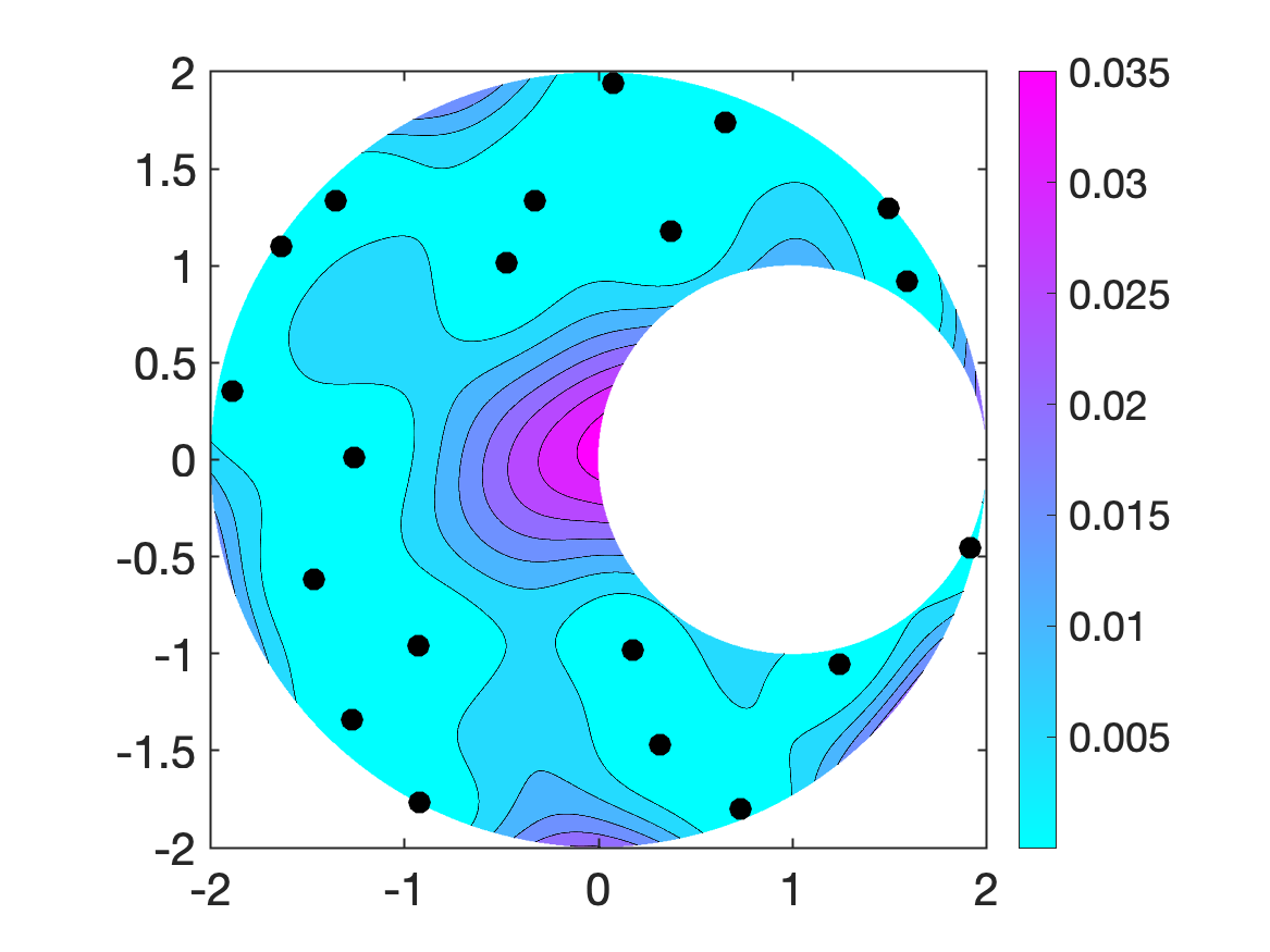
RPCholesky sampling is more flexible than many kernel quadrature methods, easily adapting to general spaces $\mathsf{X}$, measures $\mu$, and kernels $k$. To demonstrate this flexibility, we apply RPCholesky to the region $\mathsf{X}$ in fig. 1(a) equipped with the Matérn $5/2$-kernel with bandwidth $2$ and the measure

$$\mathrm{d}\mu(x,y)=(x^{2}+y^{2})\,\mathrm{d}x\,\mathrm{d}y.$$ (7)

A set of $n=20$ quadrature nodes produced by RPCholesky sampling (using algorithm 2) is shown in fig. 1(a). The cyan–pink shading shows the diagonal of the kernel after updating for the selected nodes. We see that near the selected nodes, the updated kernel is very small, meaning that future steps of the algorithm will avoid choosing nodes in those regions. Nodes far from any currently selected nodes have a much larger kernel value, making them more likely to be chosen in future RPCholesky iterations.

(a)

(b)

Figure 1: RPCholesky kernel quadrature on oddly shaped region. Left: Black dots show 20 points selected by RPCholesky on a crescent-shaped region. Shading shows kernel values $k((x,y),(x,y))$ after removing influence of selected points. Right: Mean relative error for RPCholesky kernel quadrature, iid kernel quadrature, and Monte Carlo quadrature for $f(x,y)=\sin(x)\exp(y)$ with 100 trials. Shaded regions show 10%/90% quantiles.

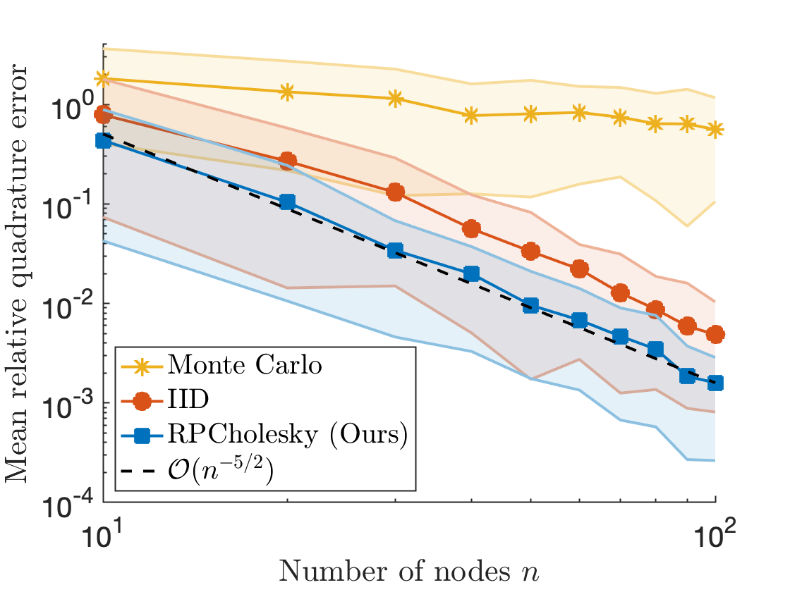
The quadrature error for $f(x,y)=\sin(x)\exp(y)$, $g\equiv 1$, and different numbers $n$ of quadrature nodes for RPCholesky kernel quadrature, kernel quadrature with nodes drawn iid from $\mu/\mu(\mathsf{X})$, and Monte Carlo quadrature are shown in fig. 1(b). Other spectrally accurate kernel quadrature methods would be difficult to implement in this setting because they would require an explicit Mercer decomposition (projection DPPs and leverage scores) or an expensive sampling procedure (continuous volume sampling). A comparison of RPCholesky with more kernel quadrature methods on a benchmark problem is provided in fig. 2.

2 Related work

Here, we overview past work on kernel quadrature and discuss the history of RPCholesky sampling.

2.1 Kernel quadrature

The goal of kernel quadrature is to provide a systematic means for designing quadrature rules on RKHS’s. Relevant points of comparison are Monte Carlo [36] and quasi-Monte Carlo [14] methods, which have $\mathcal{O}(1/\sqrt{n})$ and $\mathcal{O}(\operatorname{polylog}(n)/n)$ convergence rates, respectively.

The literature on probabilistic and kernel approaches to quadrature is vast, so any short summary is necessarily incomplete. Here, we briefly summarize some of the most prominent kernel quadrature methods, highlighting limitations that we address with our RPCholesky approach. We refer the reader to [22, Tab. 1] for a helpful comparison of many of the below-discussed methods.

Herding.

Kernel herding schemes [11, 4, 41, 26] iteratively select quadrature nodes using a greedy approach. These methods face two limitations. First, they require the solution of a (typically) nonconvex global optimization problem at every step, which may be computationally costly. Second, these methods exhibit slow $\mathcal{O}(1/n)$ quadrature error rates [11, Prop. 4] (or even slower [16]). Optimally weighted herding is known as sequential Bayesian quadrature [26].

Thinning.

Thinning methods [17, 18, 38] try to select $n$ good quadrature nodes from a larger set of $N\gg n$ candidate nodes drawn from a simple distribution. While these methods have other desirable theoretical properties, they do not benefit from spectral accuracy.

Leverage scores and projection DPPs.

With optimal weights (section 3.2), quadrature with nodes sampled using a projection determintal point process (DPP) [7] (see also [21, 5, 6]) or iid from the (ridge) leverage score distribution [3] achieve spectral accuracy. However, known efficient sampling algorithms require access to the Mercer decomposition 2, limiting the applicability of these schemes to simple spaces $\mathsf{X}$, measures $\mu$, and kernels $k$, where the decomposition is known analytically.

Continuous volume sampling.

Continuous volume sampling is the continuous analog of $n$-DPP sampling [28], providing quadrature nodes that achieve spectral accuracy [8, Prop. 5]. Unfortunately, continuous volume sampling is computationally challenging. In the finite setting, the best-known algorithm [9] for exact $n$-DPP sampling requires a costly $\mathcal{O}(|\mathsf{X}|\cdot n^{6.5}+n^{9.5})$ operations. Inexact samplers based on Markov chain Monte Carlo (MCMC) (e.g., [2, 1, 34]) may be more competitive, but the best-known samplers in the continuous setting still require an expensive $\mathcal{O}(n^{5}\log n)$ MCMC steps [34, Thms. 1.3–1.4]. RPCholesky sampling achieves similar theoretical guarantees to continuous volume sampling (see theorem 1) and can be efficiently and exactly sampled (algorithm 2).

Recombination and convex weights.

The paper [22] (see also [23]) proposes two ideas for kernel quadrature when $\mu$ is a probability measure and $g\equiv 1$. First, they suggest using a recombination algorithm (e.g., [29]) to subselect good quadratures from $N\gg n$ candidate nodes iid sampled from $\mu$. All of the variants of their method either fail to achieve spectral accuracy or require an explicit Mercer decomposition [22, Tab. 1]. Second, they propose choosing weights $(w_{1},\ldots,w_{n})$ that are convex combination coefficients. This choice makes the quadrature scheme robust against misspecification of the RKHS $\mathcal{H}\not\ni f$, among other benefits. It may be worth investigating a combination of RPCholesky quadrature nodes with convex weights in future work.

2.2 Randomly pivoted Cholesky

RPCholesky was proposed, implemented, and analyzed in [10] for the task of approximating an $M\times M$ positive-semidefinite matrix $\boldsymbol{A}$. The algorithm is algebraically equivalent to applying an earlier algorithm known as adaptive sampling [12, 13] to $\boldsymbol{A}^{1/2}$. Despite their similarities, RPCholesky and adaptive sampling are different algorithms: To produce a rank-$n$ approximation to an $M\times M$ matrix, RPCholesky requires $\mathcal{O}(n^{2}M)$ operations, while adaptive sampling requires a much larger $\mathcal{O}(nM^{2})$ operations. See [10, §4.1] for further discussion on RPCholesky’s history. In this paper, we introduce a continuous extension of RPCholesky and analyze its effectiveness for kernel quadrature.

3 Theoretical results

In this section, we prove our main theoretical result for RPCholesky kernel quadrature. We first establish the mathematical setting (section 3.1) and introduce kernel quadrature (section 3.2). Then, we present our main theorem (section 3.3) and discuss its proof (section 3.4).

3.1 Mathematical setting and notation

Let $\mu$ be a Borel measure supported on a topological space $\mathsf{X}$ and let $\mathcal{H}$ be a RKHS on $\mathsf{X}$ with continuous kernel $k:\mathsf{X}\times\mathsf{X}\to\real$. We assume that $x\mapsto k(x,x)$ is integrable 3 and that $\mathcal{H}$ is dense in $\mathsf{L}^{2}(\mu)$. These assumptions imply that $\mathcal{H}$ is compactly embedded in $\mathsf{L}^{2}(\mu)$, the Mercer decomposition 2 converges pointwise, and the Mercer eigenfunctions form an orthonormal basis of $\mathsf{L}^{2}(\mu)$ and an orthogonal basis of $\mathcal{H}$ [39, Thm. 3.1].

Define the integral operator

$$Tf(x)=\int_{\mathsf{X}}k(x,y)f(y)\,\mathrm{d}\mu(y).$$ (8)

Viewed as an operator $T:\mathsf{L}^{2}(\mu)\to\mathsf{L}^{2}(\mu)$, $T$ is self-adjoint, positive semidefinite, and trace-class.

One final piece of notation: For a function $\delta:\mathsf{X}\to\real$ and an ordered (multi)set $\mathsf{S}=\{s_{1},\ldots,s_{n}\}$, we let $\delta(\mathsf{S})$ be the column vector with $i$th entry $\delta(s_{i})$. Similarly, for a bivariate function $h:\mathsf{X}\times\mathsf{X}\to\real$, $h(\cdot,\mathsf{S})$ (resp. $h(\mathsf{S},\cdot)$) denotes the row (resp. column) vector-valued function with $i$th entry $h(\cdot,s_{i})$ (resp. $h(s_{i},\cdot)$), and $h(\mathsf{S},\mathsf{S})$ denotes the matrix with $ij$ entry $h(s_{i},s_{j})$.

3.2 Kernel quadrature

Following earlier works (e.g., [3, 7]), let us describe the kernel quadrature problem more precisely. Given a function $g\in\mathsf{L}^{2}(\mu)$, we seek quadrature weights $\boldsymbol{w}=(w_{1},\ldots,w_{n})\in{}^{n}$ and nodes $\mathsf{S}=\{s_{1},\ldots,s_{n}\}\subseteq\mathsf{X}$ that minimize the maximum quadrature error over all $f\in\mathcal{H}$ with $\left\|f\right\|_{\mathcal{H}}\leq 1$:

$$\mathrm{Err}(\mathsf{S},\boldsymbol{w};g)\coloneqq\max_{\left\|f\right\|_{\mathcal{H}}\leq 1}\left|\int_{\mathsf{X}}f(x)g(x)\,\mathrm{d}\mu(x)-\sum_{i=1}^{n}w_{i}f(s_{i})\right|.$$ (9)

A short derivation ([3, Eq. (7)] or LABEL:sec:derivation) yields the simple formula

$$\mathrm{Err}(\mathsf{S},\boldsymbol{w};g)=\left\|Tg-\sum_{i=1}^{n}w_{i}k(\cdot,s_{i})\right\|_{\mathcal{H}}.$$ (10)

This equation reveals that the quadrature rule minimizing $\mathrm{Err}(\mathsf{S},\boldsymbol{w};g)$ is the least-squares approximation of $Tg\in\mathcal{H}$ by a linear combination of kernel function evaluations $\sum_{i=1}^{n}w_{i}k(\cdot,s_{i})$.

If we fix the quadrature nodes $\mathsf{S}=\{s_{1},\ldots,s_{n}\}$, the optimal weights $\boldsymbol{w}_{\star}=(w_{\star 1},\ldots,w_{\star n})\in{}^{n}$ minimizing $\mathrm{Err}(\mathsf{S},\boldsymbol{w};g)$ are the solution of the linear system of equations

$$k(\mathsf{S},\mathsf{S})\boldsymbol{w}_{\star}=Tg(\mathsf{S}).$$ (11)

We use 11 to select the weights throughout this paper, and denote the error with optimal weights by

$$\mathrm{Err}(\mathsf{S};g)\coloneqq\mathrm{Err}(\mathsf{S},\boldsymbol{w}_{\star};g).$$ (12)

3.3 Error bounds for randomly pivoted Cholesky kernel quadrature

Our main result for RPCholesky kernel quadrature is as follows:

Theorem 1.

Let $\mathsf{S}=\{s_{1},\ldots,s_{n}\}$ be generated by the RPCholesky sampling algorithm. For any function $g\in\mathsf{L}^{2}(\mu)$, nonnegative integer $r\geq 0$, and real number $\delta>0$, we have

$$\operatorname{\mathbb{E}}\mathrm{Err}^{2}(\mathsf{S};g)\leq\delta\cdot\left\|g\right\|_{\mathsf{L}^{2}(\mu)}^{2}\cdot\sum_{i=r+1}^{\infty}\lambda_{i}$$ (13)

provided

$$n\geq r\log\left(\frac{2\lambda_{1}}{\delta\sum_{i=r+1}^{\infty}\lambda_{i}}\right)+\frac{2}{\delta}.$$ (14)

To illustrate this result, consider an RKHS with eigenvalues $\lambda_{i}=\mathcal{O}(i^{-2s})$ for $s>1/2$. An example is the periodic Sobolev space $H^{s}_{\rm per}([0,1])$ (see section 5). By setting $\delta=1/r$, we see that

$$\operatorname{\mathbb{E}}\mathrm{Err}^{2}(\mathsf{S};g)\leq\mathcal{O}(r^{-2s})\left\|g\right\|_{\mathsf{L}^{2}(\mu)}^{2}\quad\text{for {RPCholesky} with }n=\Omega(r\log r).$$ (15)

The optimal scheme requires $n=\Theta(r)$ nodes to achieve this bound [8, Prop. 5 & §2.5]. Thus, to achieve an error of $\mathcal{O}(r^{-2s})$, RPCholesky requires just logarithmically more nodes than the optimal quadrature scheme for such spaces. This compares favorably to continuous volume sampling, which achieves the slightly better optimal rate but is much more difficult to sample.

Having established that RPCholesky achieves nearly optimal error rates for interesting RKHS’s, we make some general comments on theorem 1. First, observe that the error depends on the sum $\sum_{i=r+1}^{\infty}\lambda_{i}$ of the tail eigenvalues. This tail sum is characteristic of spectrally accurate kernel quadrature schemes [7, 8]. The more distinctive feature in 14 is the logarithmic factor. Fortunately, for double precision computation, the achieveable accuracy is bounded by the machine precision $2^{-52}$, so this logarithmic factor is effectively a modest constant:

$$\log\left(\frac{2\lambda_{1}}{\delta\sum_{i=r+1}^{\infty}}\right)\lessapprox\log(2^{52})<37.$$ (16)

3.4 Connection to Nyström approximation and idea of proof

We briefly outline the proof of theorem 1. Following previous works (e.g., [3, 23]), we first utilize the connection between kernel quadrature and the Nyström approximation [31, 42] of the kernel $k$.

Definition 2.

For nodes $\mathsf{S}=\{s_{1},\ldots,s_{n}\}\subseteq\mathsf{X}$, the Nyström approximation to the kernel $k$ is

$$k_{\mathsf{S}}(x,y)=k(x,\mathsf{S})\,k(\mathsf{S},\mathsf{S})^{\dagger}\,k(\mathsf{S},y).$$ (17)

Here, ^† denotes the Moore–Penrose pseudoinverse. The Nyström approximate integral operator is

$$T_{\mathsf{S}}f\coloneqq\int_{\mathsf{X}}k_{\mathsf{S}}(\cdot,x)f(x)\,\mathrm{d}\mu(x).$$ (18)

This definition leads to a formula for the quadrature rule $\sum_{i=1}^{n}w_{i}k(\cdot,s_{i})$ with optimal weights 11.

Proposition 3.

Fix nodes $\mathsf{S}=\{s_{1},\ldots,s_{n}\}$. With the optimal weights $\boldsymbol{w}_{\star}\in{}^{n}$ 11, we have

$$\sum_{i=1}^{n}w_{i\star}k(\cdot,s_{i})=T_{\mathsf{S}}g.$$ (19)

Consequently,

$$\mathrm{Err}^{2}(\mathsf{S};g)=\left\|(T-T_{\mathsf{S}})g\right\|_{\mathcal{H}}^{2}\leq\langle g,(T-T_{\mathsf{S}})g\rangle_{\mathsf{L}^{2}(\mu)}.$$ (20)

To finish the proof of theorem 1, we develop and solve a recurrence for an upper bound on the largest eigenvalue of $\operatorname{\mathbb{E}}[T-T_{\mathsf{S}}]$. See LABEL:sec:proof_of_rpc for details and for the proof of proposition 3.

4 Efficient randomly pivoted Cholesky by rejection sampling

To efficiently perform RPCholesky sampling in the continuous setting, we can use rejection sampling. (A similar rejection sampling idea is used in the MCMC continuous volume sampler of [34].) Assume for simplicity that the measure $\mu$ is normalized so that

$$\int_{\mathsf{X}}k(x,x)\,\mathrm{d}\mu(x)=\operatorname{Tr}T=1.$$ (21)

We assume two forms of access to the kernel $k$:

1. Entry evaluations. For any $x,y\in\mathsf{X}$, we can evaluate $k(x,y)$.

2. Sampling the diagonal. We can produce samples from the measure $k(x,x)\,\mathrm{d}\mu(x)$.

To sample from the RPCholesky distribution, we use $k(x,x)\,\mathrm{d}\mu(x)$ as a proposal distribution and accept proposal $s$ with probability

$$1-\frac{k_{\mathsf{S}}(s,s)}{k(s,s)}.$$ (22)

(Recall $k_{\mathsf{S}}$ from 17.) The resulting algorithm for RPCholesky sampling is shown in algorithm 2.

Algorithm 2 RPCholesky with rejection sampling

1:Kernel $k:\mathsf{X}\times\mathsf{X}\to\real$ and number of quadrature points $n$

2:Quadrature points $s_{1},\ldots,s_{n}$

3:Initialize $\boldsymbol{L}\leftarrow\boldsymbol{0}_{n\times n}$, $i\leftarrow 1$, $\mathsf{S}\leftarrow\emptyset$ $\triangleright$ $\boldsymbol{L}$ stores a Cholesky decomposition of $k(\mathsf{S},\mathsf{S})$

4:while $i\leq n$ do

5:     Sample $s_{i}$ from the probability measure $k(x,x)\,\mathrm{d}\mu(x)$

6:     $(d,\boldsymbol{c})\leftarrow\textsc{ResidualKernel}(s_{i},\mathsf{S},\boldsymbol{L},k)$ $\triangleright$ Helper subroutine algorithm 3

7:     Draw a uniform random variable $U\sim\operatorname{\textsc{Unif}}[0,1]$

8:     if $U<d/k(s_{i},s_{i})$ then $\triangleright$ Accept with probability $d/k(s_{i},s_{i})$

9:         Induct $s_{i}$ into the selected set: $\mathsf{S}\leftarrow\mathsf{S}\cup\{s_{i}\}$, $i\leftarrow i+1$

10:         $\boldsymbol{L}(i,1:i)\leftarrow\begin{bmatrix}\boldsymbol{c}^{\top}&\sqrt{d}\end{bmatrix}$

11:     end if

12:end while

Algorithm 3 Helper subroutine to evaluate residual kernel

1:Point $s\in\mathsf{X}$, set $\mathsf{S}\subseteq\mathsf{X}$, Cholesky factor $\boldsymbol{L}$ of $k(\mathsf{S},\mathsf{S})$, and kernel $k$

2:$d=k(s,s)-k_{\mathsf{S}}(s,s)$ and $\boldsymbol{c}=\boldsymbol{L}^{-1}k(\mathsf{S},s)$

3:procedure ResidualKernel($s$,$\mathsf{S}$,$\boldsymbol{L}$,$k$)

4:     $\boldsymbol{c}\leftarrow\boldsymbol{L}^{-1}k(\mathsf{S},s)$

5:     $d\leftarrow k(s,s)-\left\|\boldsymbol{c}\right\|^{2}$ $\triangleright$ $d=k(s,s)-k_{\mathsf{S}}(s,s)$

6:     return $(d,\boldsymbol{c})$

7:end procedure

Theorem 4.

Algorithm 2 produces exact RPCholesky samples. Let $\eta_{i}$ denote the trace-error of the best rank-$i$ approximation to $T$:

$$\eta_{i}=\sum_{j=i+1}^{\infty}\lambda_{i}.$$ (23)

The expected runtime of algorithm 2 is at most $\mathcal{O}(\sum_{i=1}^{n}i^{2}/\eta_{i})\leq\mathcal{O}(n^{3}/\eta_{n-1})$.

This result demonstrates that algorithm 2 suffers from the curse of smoothness: The faster the eigenvalues $\lambda_{1},\lambda_{2},\ldots$ decrease, the smaller $\eta_{n-1}$ will be and, consequently, the slower algorithm 2 will be in expectation. While this curse is an unfortunate limitation, it is also a common one. The curse of smoothness affects all known Mercer-free, spectrally accurate kernel quadrature schemes. In fact, the situation is worse for other algorithms. The CVS sampler of [34], for example, requires as many as $\mathcal{O}(n^{5}\log n)$ MCMC steps, each of which has cost $\mathcal{O}(n^{2}/\eta_{n-1})$. According to current analysis, algorithm 2 is $\mathcal{O}(n^{4}\log n)$-times faster than the CVS sampler of [34].

Notwithstanding the curse of smoothness, algorithm 2 is useful in practice. The algorithm works under minimal assumptions and can reach useful accuracies $\eta=10^{-5}$ while sampling $n=1000$ nodes on a laptop. Algorithm 2 may also be interesting for RPCholesky sampling for a large finite set $|\mathsf{X}|\geq 10^{9}$, since its runtime has no explicit dependence on the size of the space $\mathsf{X}$.

To achieve higher accuracies and blunt the curse of smoothness, we can improve algorithm 2 with optimization. Indeed, the optimal acceptance probability for algorithm 2 would be

$$p(s_{i};\alpha)=\frac{1}{\alpha}\cdot\frac{k(s_{i},s_{i})-k_{\mathsf{S}}(s_{i},s_{i})}{k(s_{i},s_{i})}\quad\text{where}\quad\alpha=\max_{x\in\mathsf{X}}\frac{k(x,x)-k_{\mathsf{S}}(x,x)}{k(x,x)}.$$ (24)

This suggests the following scheme: Initialize with $\alpha=1$ and run the algorithm with acceptance probability $p(s_{i};\alpha)$. If we perform many loop iterations without an acceptance, we then recompute the optimal $\alpha$ by solving an optimization problem. The resulting procedure is shown in algorithm 4.

Algorithm 4 RPCholesky with optimized rejection sampling

1:Kernel $k:\mathsf{X}\times\mathsf{X}\to\real$ and number of quadrature points $n$

2:Quadrature points $s_{1},\ldots,s_{n}$

3:Initialize $\boldsymbol{L}\leftarrow\boldsymbol{0}_{n\times n}$, $i\leftarrow 1$, $\mathsf{S}\leftarrow\emptyset$, $\mathtt{trials}\leftarrow 0$, $\alpha\leftarrow 1$

4:while $i\leq n$ do

5:     $\mathtt{trials}\leftarrow\mathtt{trials}+1$

6:     Sample $s_{i}$ from the probability measure $k(x,x)\,\mathrm{d}\mu(x)$

7:     $(d,\boldsymbol{c})\leftarrow\textsc{ResidualKernel}(s_{i},\mathsf{S},\boldsymbol{L},k)$ $\triangleright$ Helper subroutine algorithm 3

8:     Draw a uniform random variable $U\sim\operatorname{\textsc{Unif}}[0,1]$

9:     if $U<(1/\alpha)\cdot d/k(s_{i},s_{i})$ then $\triangleright$ Accept with probability $d/k(s_{i},s_{i})$

10:         $\mathsf{S}\leftarrow\mathsf{S}\cup\{s_{i}\}$, $i\leftarrow i+1$, $\mathtt{trials}\leftarrow 0$

11:         $\boldsymbol{L}(i,1:i)\leftarrow\begin{bmatrix}\boldsymbol{c}^{\top}&\sqrt{d}\end{bmatrix}$

12:     end if

13:     if $\mathtt{trials}\geq\mathtt{TRIALS\_MAX}$ then $\triangleright$ We use $\mathtt{TRIALS\_MAX}\in[25,1000]$

14:         $\alpha\leftarrow\max_{x\in\mathsf{X}}\textsc{ResidualKernel}(x,\mathsf{S},\boldsymbol{L},k)/k(x,x)$

15:         $\mathtt{trials}\leftarrow 0$

16:     end if

17:end while

If the optimization problem for $\alpha$ is solved to global optimality, then algorithm 4 produces exact RPCholesky samples. The downside of algorithm 4 is the need to solve a (typically) nonconvex global optimization problem to compute the optimal $\alpha$. Fortunately, in our experiments (section 5), only a small number of optimization problems ($\leq 10$) are needed to produce a sample of $n=1000$ nodes. In the setting where the optimization problem is tractable, the speedup of algorithm 4 can be immense. To produce $n=200$ RPCholesky samples for the space $[0,1]^{3}$ with the kernel 26, algorithm 4 requires just $0.19$ seconds compared to $7.47$ seconds for algorithm 2.

5 Comparison of methods on a benchmark example

Having demonstrated the versatility of RPCholesky for general spaces $\mathsf{X}$, measures $\mu$, and kernels $k$ in fig. 1, we now present a benchmark example from the kernel quadrature literature to compare RPCholesky with other methods. Consider the periodic Sobolev space $H^{s}_{\rm per}([0,1])$ with kernel

$$k(x,y)=1+2\sum_{m=1}^{\infty}m^{-2s}\cos(2\pi m(x-y))=1+\frac{(-1)^{s-1}(2\pi)^{2s}}{(2s)!}B_{2s}(\{x-y\}),$$ (25)

where $B_{2s}$ is the $(2s)$th Bernoulli polynomial and $\{\cdot\}$ reports the fractional part of a real number [3, p. 7]. We also consider $[0,1]^{3}$ equipped with the product kernel

$$k^{\otimes 3}((x_{1},x_{2},x_{3}),(y_{1},y_{2},y_{3}))=k(x_{1},y_{1})k(x_{2},y_{2})k(x_{3},y_{3}).$$ (26)

We quantify the performance of nodes $\mathsf{S}$ and weights $\boldsymbol{w}$ using $\mathrm{Err}(\mathsf{S},\boldsymbol{w};g)$, which can be computed in closed form [22, Eq. (14)]. We set $\mu\coloneqq\operatorname{\textsc{Unif}}[0,1]^{d}$ and $g\equiv 1$.

We compare the following schemes:

• Monte Carlo, IID kernel quadrature. Nodes $s_{1},\ldots,s_{n}\stackrel{{\scriptstyle\mathrm{iid}}}{{\sim}}\mu$ with uniform weights $w_{i}=1/n$ (Monte Carlo) and optimal weights 11 (IID).

• Thinning. Nodes $s_{1},\ldots,s_{n}$ thinned from $n^{2}$ iid samples from $\mu=\operatorname{\textsc{Unif}}[0,1]$ using kernel thinning [17, 18] with the Compress++ algorithm [38] with optimal weights 11.

• Continuous volume sampling (CVS). Nodes $s_{1},\ldots,s_{n}$ drawn from the volume sampling distribution [8, Def. 1] by Markov chain Monte Carlo with optimal weights 11.

• RPCholesky. Nodes $s_{1},\ldots,s_{n}$ sampled by RPCholesky using algorithm 4 with the optimal weights 11.

• Positively weighted kernel quadrature (PWKQ). Nodes and weights computed by the Nyström+empirical+opt method as described on [22, p. 9].

See LABEL:sec:numerical_experiment_details for more details about our numerical experiments. Experiments were run on a MacBook Pro with a 2.4 GHz 8-Core Intel Core i9 CPU and 64 GB 2667 MHz DDR4 RAM. Our code is available at https://github.com/eepperly/RPCholesky-Kernel-Quadrature.

(a) $s=3$, $d=1$

(b) $s=3$, $d=3$

Figure 2: Benchmark example: Sobolev space. Mean quadrature error $\mathrm{Err}(\mathsf{S},\boldsymbol{w};g)$ (left) and sampling time (right) for different methods (100 trials) for $s=1$, $d=3$ (top) and $s=d=3$ (bottom). Shaded regions show 10%/90% quantiles.

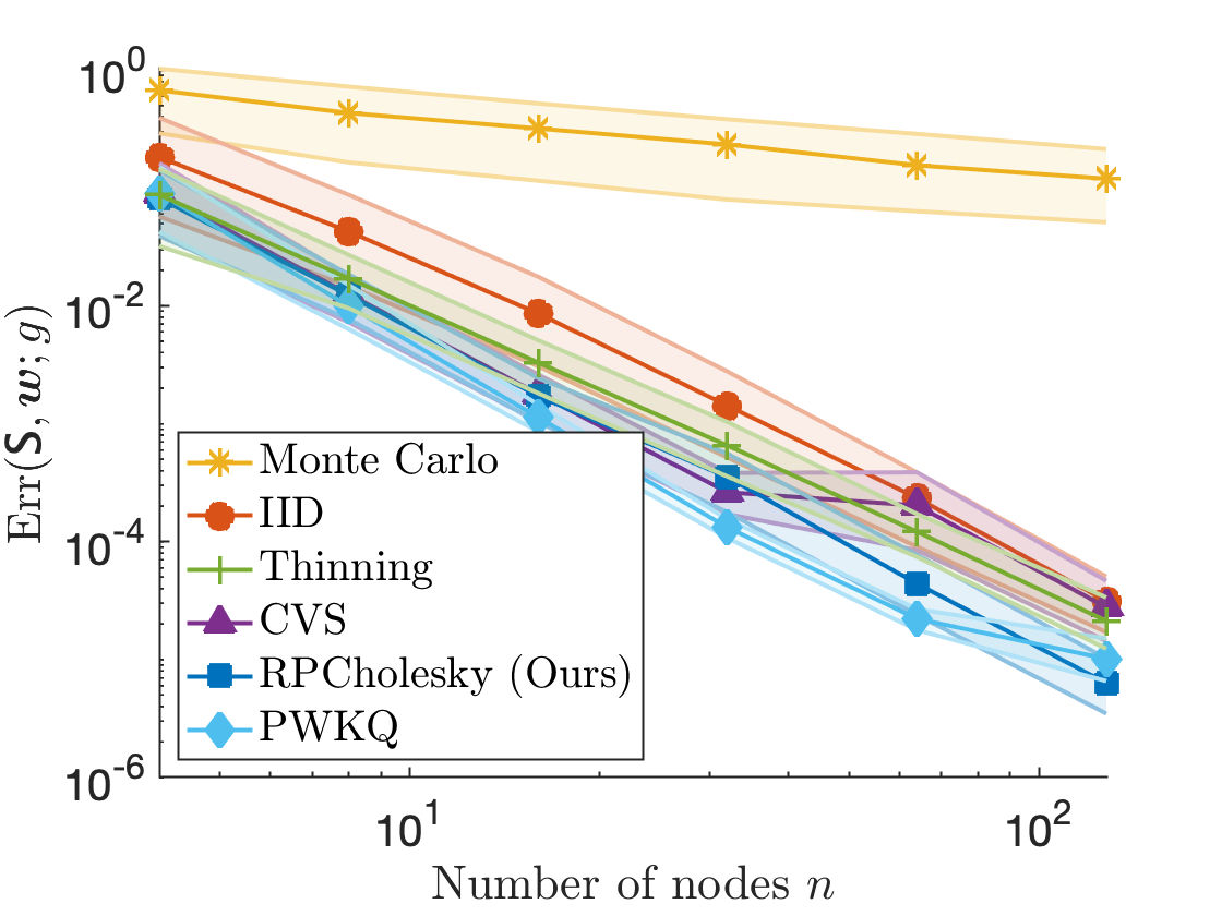
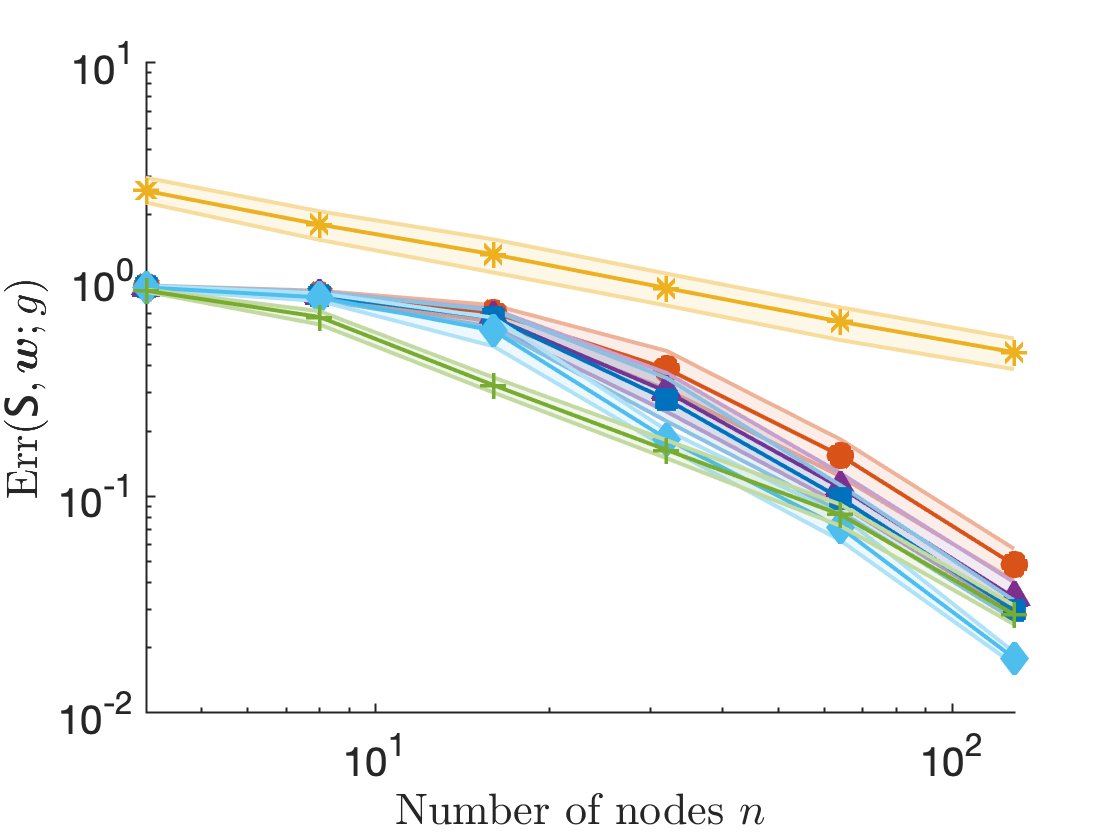
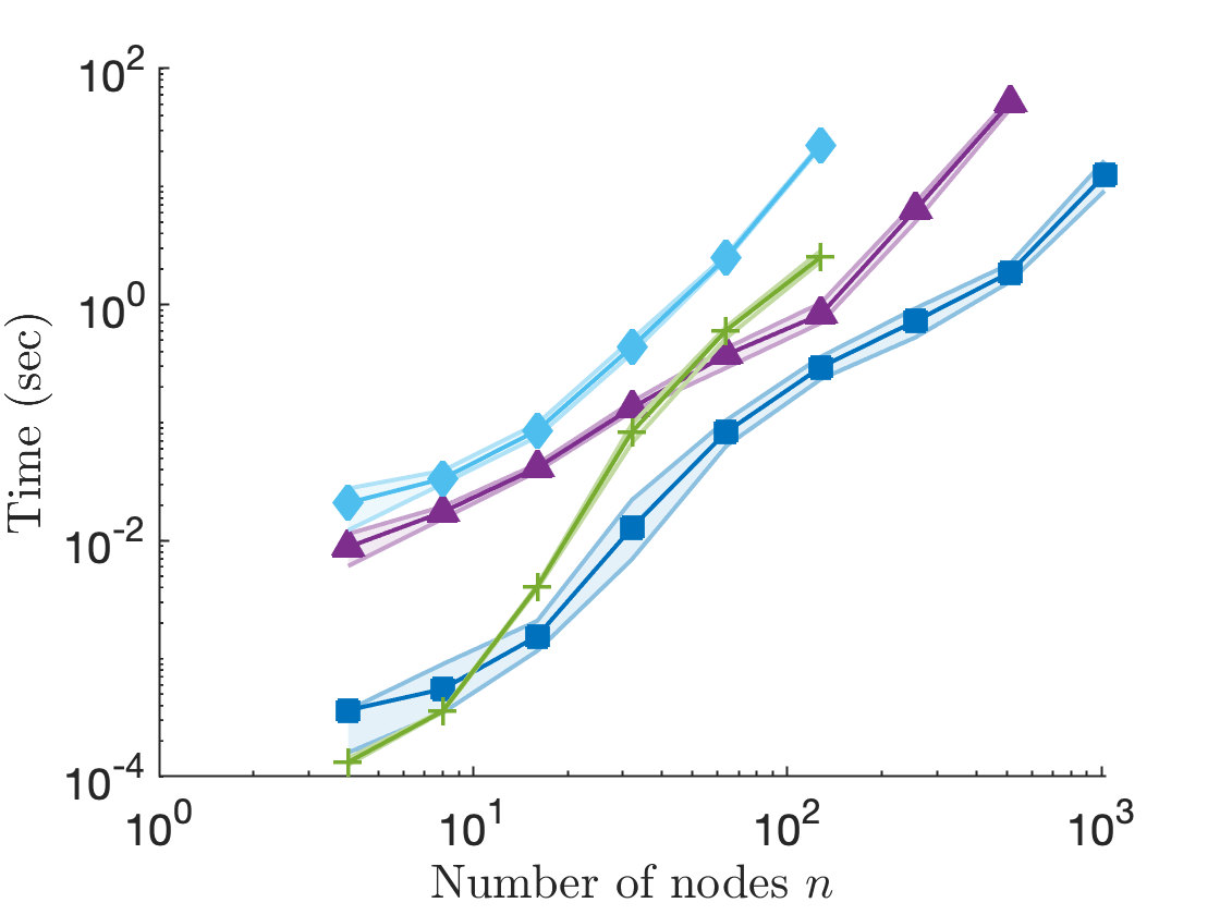
Errors for the different methods are shown in fig. 2 (left panels). We see that RPCholesky consistently performs among the best methods at every value of $n$, numerically achieving the rate of convergence of the fastest method for each problem. Particularly striking is the result that RPCholesky sampling’s performance is either very close to or better than that of continuous volume sampling, despite the latter’s slightly stronger theoretical properties.

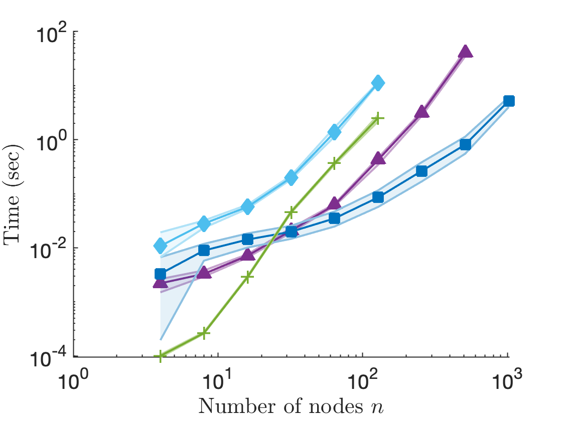
Figure 2 (right panels) show the sampling times for each of the nonuniform sampling methods. RPCholesky sampling is the fastest by far. To sample 128 nodes for $s=3$ and $d=1$, RPCholesky was 17$\times$ faster than continuous volume sampling, 52$\times$ faster than thinning, and 170$\times$ faster than PWKQ.

To summarize our numerical evaluation (comprising fig. 2 and fig. 1 from the introduction), we find that RPCholesky is among the most accurate kernel quadrature methods tested. To us, the strongest benefits of RPCholesky (supported by these experiments) are the method’s speed and flexibility. These virtues make it possible to apply spectrally accurate kernel quadrature in scenarios where it would have been computationally intractable before.

6 Application: Analyzing large chemistry datasets

While our focus thusfar has been on infinite domains $\mathsf{X}$, the kernel quadrature formalism can also be applied to a finite set $\mathsf{X}$ of data points. Let $\mu=\operatorname{\textsc{Unif}}\mathsf{X}$ be the uniform distribution and set $g\equiv 1$. Here, the task is to exhibit $n$ nodes $\mathsf{S}=\{s_{1},\ldots,s_{n}\}\subseteq\mathsf{X}$ and weights $\boldsymbol{w}\in{}^{n}$ such that the average of every “smooth” function $f:\mathsf{X}\to\real$ over the whole dataset is well-approximated by a sum:

$$\operatorname{mean}(f)\coloneqq\frac{1}{|\mathsf{X}|}\sum_{x\in\mathsf{X}}f(x)\approx\sum_{i=1}w_{i}f(s_{i}).$$ (27)

Here is an application to chemistry. Let $\mathsf{X}$ denote a large set of compounds of interest, and let $f:\mathsf{X}\to\real$ denote a target chemical property such as specific heat capacity. We are interested in computing $\operatorname{mean}(f)$. Unfortunately, evaluating $f$ on each $x\in\mathsf{X}$ requires an expensive density functional theory computation, so it can be prohibitively expensive to evaluate $f$ on every $x\in\mathsf{X}$. Fortunately, we can obtain fast approximations to $\operatorname{mean}(f)$ using 27, which only require evaluating $f$ on a much smaller set of size $|\mathsf{S}|\ll|\mathsf{X}|$.

Our experimental setup is as follows. For $\mathsf{X}$, we use $2\times 10^{4}$ randomly selected points from the QM9 dataset [37, 33, 40]. We represent each compound as a vector in ¹⁵⁰⁰ using the many-body tensor representation [25] computed with the DScribe package [24]. Choose $k$ to be a Gaussian kernel with bandwidth chosen by median heuristic [20] on a further subsample of $10^{3}$ random points. We omit continuous volume sampling, thinning, and positively weighted kernel quadrature because of their computational cost. In their place, we add the greedy Nyström method [19] with optimal weights 11.

(a)

(b)

Figure 3: Application: chemistry. Worst-case quadrature error (left) and mean relative error for estimation of the average value of the isotropic polarizability function $f(x)$ (right) for different methods (100 trials). Shaded regions show 10%/90% quantiles.

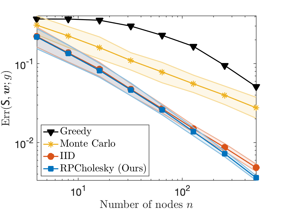
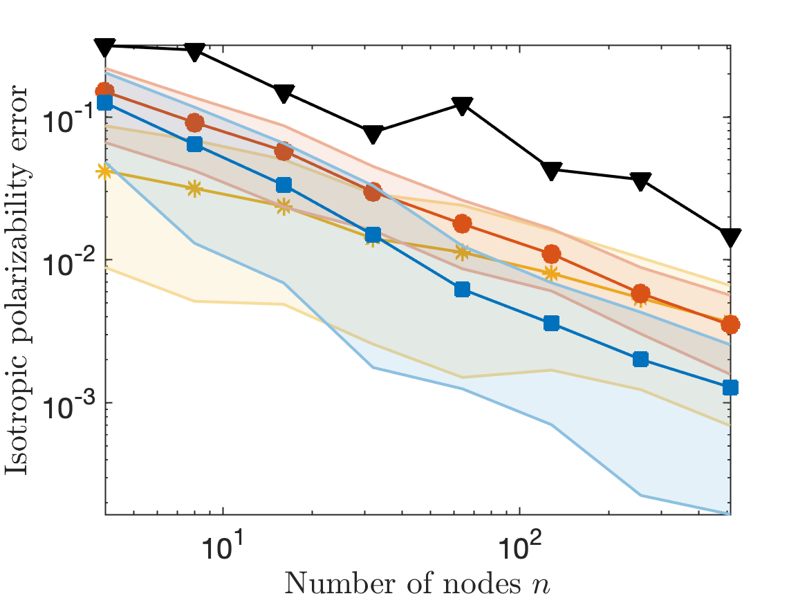
Results are shown in fig. 3. Figure 3(a) shows the worst-case quadrature error 12. For this metric, IID and randomly pivoted Cholesky are the definitive winners, with randomly pivoted Cholesky being slightly better. Figure 3(b) shows the mean relative error for the kernel quadrature estimates of the mean isotropic polarizability of the compounds in $\mathsf{X}$. For sufficiently large $n$, randomly pivoted Cholesky has the smallest error, beating IID and Monte Carlo by a factor of three at $n=512$.

7 Conclusions, Limitations, and Possibilites for Future Work

In this article, we developed continuous RPCholesky sampling for kernel quadrature. Theorem 1 demonstrates RPCholesky kernel quadrature achieves near-optimal error rates. Numerical results (fig. 2) hint that its practical performance might be even better than that suggested by our theoretical analysis and fully comparable with kernel quadrature based on the much more computationally expensive continuous volume sampling distribution. RPCholesky supports performant rejection sampling algorithms (algorithms 2 and 4), which facilitate implementation for general spaces $\mathsf{X}$, measures $\mu$, and kernels $k$ with ease.

We highlight three limitations of RPCholesky kernel quadrature that would be worth addressing in future work. First, given the comparable performance of RPCholesky and continuous volume sampling in practice, it would be desirable to prove stronger error bounds for RPCholesky sampling or find counterexamples which demonstrate a separation between the methods. Second, it would be worth developing improved sampling algorithms for RPCholesky which avoid the need for global optimization steps. Third, all known spectrally accurate kernel quadrature methods require integrals of the form $\int_{\mathsf{X}}k(x,y)g(y)\,\mathrm{d}\mu(y)$, which may not be available. RPCholesky kernel quadrature requires them for the computation of the weights 11. Developing spectrally accurate kernel quadrature schemes that avoid such integrals remains a major open problem for the field.

References

- [1] Nima Anari, Yang P. Liu, and Thuy-Duong Vuong. Optimal sublinear sampling of spanning trees and determinantal point processes via average-case entropic independence. In 63rd Annual Symposium on Foundations of Computer Science, pages 123–134. IEEE, October 2022.
- [2] Nima Anari, Shayan Oveis Gharan, and Alireza Rezaei. Monte Carlo Markov chain algorithms for sampling strongly Rayleigh distributions and determinantal point processes. In Proceedings of the 29th Conference on Learning Theory, pages 103–115. PMLR, June 2016.
- [3] Francis Bach. On the equivalence between kernel quadrature rules and random feature expansions. Journal of Machine Learning Research, 18(1):714–751, January 2017.
- [4] Francis Bach, Simon Lacoste-Julien, and Guillaume Obozinski. On the equivalence between herding and conditional gradient algorithms. Proceedings of the 29th International Conference on Machine Learning, March 2012.
- [5] Rémi Bardenet and Adrien Hardy. Monte Carlo with determinantal point processes. The Annals of Applied Probability, 30(1):368–417, February 2020.
- [6] Ayoub Belhadji. An analysis of Ermakov–Zolotukhin quadrature using kernels. In Advances in Neural Information Processing Systems, volume 34, pages 27278–27289. Curran Associates, Inc., 2021.
- [7] Ayoub Belhadji, Rémi Bardenet, and Pierre Chainais. Kernel quadrature with DPPs. In Advances in Neural Information Processing Systems, volume 32. Curran Associates, Inc., 2019.
- [8] Ayoub Belhadji, Rémi Bardenet, and Pierre Chainais. Kernel interpolation with continuous volume sampling. In Proceedings of the 37th International Conference on Machine Learning, pages 725–735. PMLR, November 2020.
- [9] Daniele Calandriello, Michal Derezinski, and Michal Valko. Sampling from a -DPP without looking at all items. In Advances in Neural Information Processing Systems, volume 33, pages 6889–6899. Curran Associates, Inc., 2020.
- [10] Yifan Chen, Ethan N. Epperly, Joel A. Tropp, and Robert J. Webber. Randomly pivoted Cholesky: Practical approximation of a kernel matrix with few entry evaluations, February 2023. arXiv:2207.06503.
- [11] Yutian Chen, Max Welling, and Alex Smola. Super-samples from kernel herding. In Proceedings of the Twenty-Sixth Conference on Uncertainty in Artificial Intelligence, page 109–116. AUAI Press, 2010.
- [12] Amit Deshpande, Luis Rademacher, Santosh Vempala, and Grant Wang. Matrix approximation and projective clustering via volume sampling. In Proceedings of the seventeenth annual ACM-SIAM symposium on Discrete algorithm, pages 1117–1126. ACM, 2006.
- [13] Amit Deshpande and Santosh Vempala. Adaptive sampling and fast low-rank matrix approximation. In Josep Díaz, Klaus Jansen, José D. P. Rolim, and Uri Zwick, editors, Approximation, Randomization, and Combinatorial Optimization. Algorithms and Techniques, pages 292–303. Springer Berlin Heidelberg, 2006.
- [14] Josef Dick and Friedrich Pillichshammer. Quasi-Monte Carlo integration, discrepancy and reproducing kernel Hilbert spaces, page 16–45. Cambridge University Press, 2010.
- [15] Tobin A. Driscoll, Nicholas Hale, and Lloyd N. Trefethen. Chebfun guide, 2014.
- [16] J. C. Dunn. Convergence rates for conditional gradient sequences generated by implicit step length rules. SIAM Journal on Control and Optimization, 18(5):473–487, 1980.
- [17] Raaz Dwivedi and Lester Mackey. Kernel thinning. In Proceedings of Thirty Fourth Conference on Learning Theory, pages 1753–1753. PMLR, August 2021.
- [18] Raaz Dwivedi and Lester Mackey. Generalized kernel thinning. In Tenth International Conference on Learning Representations, April 2022.
- [19] Shai Fine and Katya Scheinberg. Efficient SVM Training training using low-rank kernel representations. Journal of Machine Learning Research, 2(Dec):243–264, 2001.
- [20] Damien Garreau, Wittawat Jitkrittum, and Motonobu Kanagawa. Large sample analysis of the median heuristic, October 2018. arXiv:1707.07269.
- [21] Guillaume Gautier, Rémi Bardenet, and Michal Valko. On two ways to use determinantal point processes for Monte Carlo integration. In Advances in Neural Information Processing Systems, volume 32. Curran Associates, Inc., 2019.
- [22] Satoshi Hayakawa, Harald Oberhauser, and Terry Lyons. Positively weighted kernel quadrature via subsampling. In Advances in Neural Information Processing Systems, volume 35, pages 6886–6900. Curran Associates, Inc., 2022.
- [23] Satoshi Hayakawa, Harald Oberhauser, and Terry Lyons. Sampling-based Nyström approximation and kernel quadrature, January 2023. arXiv:2301.09517.
- [24] Lauri Himanen, Marc O. J. Jäger, Eiaki V. Morooka, Filippo Federici Canova, Yashasvi S. Ranawat, David Z. Gao, Patrick Rinke, and Adam S. Foster. DScribe: Library of descriptors for machine learning in materials science. Computer Physics Communications, 247:106949, February 2020.
- [25] Haoyan Huo and Matthias Rupp. Unified representation of molecules and crystals for machine learning. Machine Learning: Science and Technology, 3:045017, November 2022.
- [26] Ferenc Huszár and David Duvenaud. Optimally-weighted herding is Bayesian quadrature. In Proceedings of the Twenty-Eighth Conference on Uncertainty in Artificial Intelligence, page 377–386. AUAI Press, 2012.
- [27] Hans Kersting and Philipp Hennig. Active uncertainty calibration in Bayesian ODE solvers. In Proceedings of the Thirty-Second Conference on Uncertainty in Artificial Intelligence, page 309–318. AUAI Press, 2016.
- [28] Alex Kulesza and Ben Taskar. -DPPs: Fixed-size determinantal point processes. In Proceedings of the 28th International Conference on Machine Learning, pages 1193–1200. Omnipress, January 2011.
- [29] C. Litterer and T. Lyons. High order recombination and an application to cubature on Wiener space. The Annals of Applied Probability, 22(4):1301–1327, August 2012.
- [30] Kevin P. Murphy. Machine Learning: A Probabilistic Perspective. The MIT Press, 2012.
- [31] E. J. Nyström. Über Die Praktische Auflösung von Integralgleichungen mit Anwendungen auf Randwertaufgaben. Acta Mathematica, 54(0):185–204, 1930.
- [32] Supratik Paul, Konstantinos Chatzilygeroudis, Kamil Ciosek, Jean-Baptiste Mouret, Michael A. Osborne, and Shimon Whiteson. Alternating optimisation and quadrature for robust control. In Proceedings of the Thirty-Second AAAI Conference on Artificial Intelligence, (AAAI-18), the 30th innovative Applications of Artificial Intelligence (IAAI-18), and the 8th AAAI Symposium on Educational Advances in Artificial Intelligence (EAAI-18), pages 3925–3933. AAAI Press, February 2018.
- [33] Raghunathan Ramakrishnan, Pavlo O. Dral, Matthias Rupp, and O. Anatole von Lilienfeld. Quantum chemistry structures and properties of 134 kilo molecules. Scientific Data, 1(1):140022, December 2014.
- [34] Alireza Rezaei and Shayan Oveis Gharan. A polynomial time MCMC method for sampling from continuous determinantal point processes. In Proceedings of the 36th International Conference on Machine Learning, pages 5438–5447. PMLR, May 2019.
- [35] Christian P. Robert. The Bayesian Choice: From Decision-Theoretic Foundations to Computational Implementation. Springer Texts in Statistics. Springer, second edition, 2007.
- [36] Christian P. Robert and George Casella. Monte Carlo Statistical Methods. Springer Texts in Statistics. Springer, second edition, 2004.
- [37] Lars Ruddigkeit, Ruud van Deursen, Lorenz C. Blum, and Jean-Louis Reymond. Enumeration of 166 billion organic small molecules in the chemical universe database GDB-17. Journal of Chemical Information and Modeling, 52(11):2864–2875, November 2012.
- [38] Abhishek Shetty, Raaz Dwivedi, and Lester Mackey. Distribution compression in near-linear time. In Tenth International Conference on Learning Representations, April 2022.
- [39] Ingo Steinwart and Clint Scovel. Mercer’s theorem on general domains: On the interaction between measures, kernels, and RKHSs. Constructive Approximation, 35(3):363–417, June 2012.
- [40] Annika Stuke, Milica Todorović, Matthias Rupp, Christian Kunkel, Kunal Ghosh, Lauri Himanen, and Patrick Rinke. Chemical diversity in molecular orbital energy predictions with kernel ridge regression. The Journal of Chemical Physics, 150(20):204121, May 2019.
- [41] Kazuma Tsuji, Ken’ichiro Tanaka, and Sebastian Pokutta. Pairwise conditional gradients without swap steps and sparser kernel herding. In Proceedings of the International Conference on Machine Learning, 2022.
- [42] Christopher K. I. Williams and Matthias Seeger. Using the Nyström method to speed up kernel machines. In Proceedings of the 13th International Conference on Neural Information Processing Systems, pages 661–667. MIT Press, January 2000.